


Abstract
Efficient container stacking in terminal yards plays a critical role in improving the sustainability and productivity of port operations, as it directly affects unproductive movements, energy consumption, and cargo flows between vessels and the hinterland. This study addresses a multi-objective container stacking problem that jointly considers operational productivity and energy efficiency of yard equipment. A scattered stacking policy can reduce container reshuffles and improve service levels, but may increase energy consumption due to longer travel distances of yard cranes and trucks. Conversely, consolidating containers within smaller yard areas can reduce energy consumption but may result in higher reshuffle rates. To capture this trade-off, two evolutionary multi-objective optimization algorithms, the Pareto Archived Evolutionary Strategy (PAES) and the Non-dominated Sorting Genetic Algorithm II (NSGA-II), are adapted to the container stacking problem through a problem-specific solution representation and tailored initialization procedures, enabling the generation of diverse sets of non-dominated solutions. Extensive computational experiments on 450 instances derived from realistic terminal layouts and operational data are conducted to compare the performance of the two algorithms. The results show that NSGA-II consistently provides higher-quality Pareto front approximations, outperforming PAES by up to 115% on average. In addition, a case study based on 30 real-world instances from the Vigo Container Terminal in Spain demonstrates that the proposed approach can reduce unproductive container movements by approximately 74% while improving energy efficiency by up to 26%, highlighting its potential to support more sustainable container terminal operations.
1. Introduction
Container terminals play a pivotal role in global supply chains by ensuring the efficient transfer of cargo between maritime and hinterland transport systems and by serving as key interchange points between sea and land operations. Containerized cargo transportation has grown by more than 8% over the past decades [1], reaching nearly 180 million twenty-foot equivalent units (TEUs) in 2025 [2]. This sustained growth has increased pressure on terminals in terms of throughput requirements, land-use constraints, and intensified competition to provide high service levels to shipping lines and cargo owners [3]. In parallel, the continued expansion of global containerized trade has encouraged shipping lines to deploy increasingly larger vessels in order to exploit economies of scale in maritime transportation. To ensure that the anticipated cost advantages of larger container ships are fully realized, container terminals must maintain high levels of productivity and operational efficiency [4]. At the same time, these productivity-focused pressures have intensified concerns regarding the environmental footprint of terminal operations, particularly energy consumption and associated emissions from yard equipment.
Container terminals operate as open systems with bidirectional cargo flows, where vessel loading and unloading activities take place at the quayside, while container exchanges with trucks or trains occur at the landside [5]. The terminal storage yard serves as a temporary buffer where containers are stored before being loaded onto vessels or retrieved by cargo consignees. Effective management of yard operations is therefore crucial for overall terminal productivity, as the yard links maritime and hinterland operations and absorbs fluctuations between them [6]. An efficient yard management strategy minimizes unproductive container moves, thereby enabling faster vessel loading and unloading operations and reducing vessel turnaround times.
One of the main advantages of containerization is that containers can be stacked vertically in the yard, allowing multiple containers (e.g., four to six) to be stored in a single stack and thereby improving space utilization. However, this storage configuration may also generate unproductive moves, known as reshuffles, when a container scheduled for retrieval, either for vessel loading or for delivery to cargo consignees, is blocked by other containers stacked above it. A reshuffle involves relocating one or more blocking containers in order to access and retrieve the target container. Reshuffles represent a major source of operational inefficiency in container terminals. For instance, He et al. [7] report that, on average, 36% of all container moves in terminals located in the Pearl River Delta region of China are reshuffles, with peak rates reaching up to 60% [7]. Since the initial stacking decisions for incoming import and export containers largely determine the number of future reshuffles, these decisions must be made carefully [8]. Beyond their operational impact, reshuffles also lead to additional crane and truck movements, resulting in higher energy consumption and carbon emissions.
Another increasingly important topic in container terminal operations management is environmental sustainability. The port and shipping industry is estimated to contribute approximately 3% of global greenhouse gas emissions [9]. Ports, as significant emission sources within maritime supply chains, generate on average up to 5.69 kg CO2 eq. per tonne of cargo handled [10]. At the port level, container vessels and tankers account for nearly 85% of total emissions [11].
Together with growing public awareness of climate change, the port industry is facing increasing pressure from local communities and regulatory institutions due to its environmental externalities, including greenhouse gas emissions, water pollution, and industrial waste [12]. Globally, reducing the environmental impact of shipping has become one of the main strategic priorities of the International Maritime Organization [13]. In response, ports have initiated a range of measures aimed at mitigating the environmental footprint of their operations. Notable collective initiatives include the World Ports Climate Initiative launched in 2008 and the subsequent World Ports Sustainability Program introduced in 2017 [14]. In addition, international standards and certification schemes such as ISO 14001, Green Ports, EMAS III, and EcoPorts have been adopted to support ports in improving their environmental performance [15].
Energy efficiency is a key instrument for terminal operators seeking to improve the environmental sustainability of their operations and is closely linked to several United Nations Sustainable Development Goals, including Affordable and Clean Energy, Industry, Innovation and Infrastructure, Climate Action [16]. Improving energy efficiency through technical and operational measures represents one of the primary strategies adopted by ports to reduce greenhouse gas emissions [9]. Typical initiatives include the integration of renewable energy sources, the electrification of terminal infrastructure and equipment (e.g., onshore power supply systems, electrified handling equipment, and energy-efficient lighting), as well as operational strategies such as energy-aware optimization of terminal processes and the reduction of peak energy demand [17,18]. However, the effectiveness of such measures critically depends on operational planning decisions that govern daily equipment movements and energy usage within the terminal.
The container stacking problem concerns the assignment of exact storage locations in the yard to inbound, outbound, and transshipment containers arriving at a container terminal [19]. An effective stacking strategy can significantly reduce future reshuffles and container retrieval times, thereby accelerating vessel loading operations and cargo collection by hinterland transport modes. A substantial body of research has examined the container stacking problem, traditionally focusing on objectives such as minimizing the (expected) number of reshuffles, reducing the travel distances of yard equipment and trucks, shortening the completion time of stacking operations, and balancing workloads across yard resources [20,21].
Energy efficiency and environmental sustainability are widely recognized as seminal research themes in green maritime logistics [22]. Nevertheless, container terminal operations research has devoted limited attention to the explicit integration of environmental objectives into operational planning models. According to the comprehensive review by [20], only 9 out of 117 studies on container terminal operations published up to 2021 incorporated environmental considerations. More recently, Raeesi et al. [23] identified 47 terminal operations optimization studies that explicitly address environmental sustainability, indicating a growing, but still relatively limited research interest in this direction.
Despite this increasing attention at the terminal level, environmental sustainability remains largely absent from the container stacking literature. The vast majority of existing studies focus primarily on minimizing the number of reshuffles, and occasionally on reducing the travel distances of yard equipment or the completion time of stacking operations. Critically, the potential trade-off between stacking strategies that enhance operational productivity by reducing reshuffles and those that improve the energy efficiency and environmental performance of yard equipment has not been explicitly investigated. Understanding this trade-off is essential for assessing the implications of energy-aware operational policies and supporting terminal operators in making informed, sustainability-oriented stacking decisions. In this context, operational decisions such as container stacking can play a direct role in reducing energy consumption and emissions, highlighting the importance of integrating sustainability considerations into terminal planning models.
We address this gap by formulating a multi-objective container stacking problem (MCSP) that explicitly captures the trade-off between operational productivity and environmental sustainability through energy efficiency. The main contributions of this paper are summarized as follows:
- We formulate a novel multi-objective container stacking problem that simultaneously minimizes the expected number of future reshuffles and the energy consumption associated with yard stacking operations.
- We adapt two evolutionary multi-objective optimization algorithms, the Pareto Archived Evolutionary Strategy (PAES) and the Non-Dominated Sorting Genetic Algorithm II (NSGA-II), to the multi-objective container stacking problem by designing a problem-specific chromosome representation and diversified population initialization procedures.
- We conduct extensive computational experiments on 450 problem instances derived from realistic terminal layouts and operational data to evaluate and compare the performance of the proposed solution methods.
- We provide a quantitative assessment of the sustainability implications of container stacking decisions by linking operational planning to energy consumption, fuel usage, and CO2 emissions.
- We demonstrate the practical relevance of the proposed approach through a real-world case study based on operational data from the Vigo Container Terminal in Spain, highlighting its potential to improve both stacking productivity and energy efficiency.
The remainder of this paper is organized as follows. Section 2 reviews the relevant literature on the container stacking problem. Section 3 formally defines the multi-objective container stacking problem. The proposed solution approaches are described in Section 4. Section 5 presents the computational experiments and discusses the results. This is followed by Section 6, which reports a real-world case study based on the Vigo Container Terminal. The limitations of the research are discussed in Section 7. Finally, concluding remarks and directions for future research are provided in Section 8.
2. Literature Review
Container terminals serve as the primary interface between maritime and inland transportation systems. They function both as transshipment points, where containers are loaded and unloaded from vessels, and as temporary storage areas before cargo is dispatched to or received from the hinterland. A typical container terminal comprises three main operational areas [3,19,21]: (1) the waterside or quayside, where vessels are berthed and containers are handled by quay cranes; (2) the storage yard, where containers are temporarily stored and organized before retrieval; and (3) the landside, where containers are transferred between the terminal and consignees via external trucks or trains (Figure 1).
Figure 1.
Layout of a typical container terminal.
The storage yard is typically organized into blocks of container stacks. Each block consists of multiple bays, where containers are arranged in vertical stacks. The vertical levels within each stack are referred to as tiers. Figure 2 illustrates a container block with six stacks, each stacked up to four tiers.
Figure 2.
A container block with six stacks and four tiers.
2.1. Container Stacking Problem
Storage space allocation for containers arriving at a terminal yard is a critical decision that directly impacts overall terminal productivity and service levels. Space allocation decisions can target either the assignment of storage areas to groups of containers (e.g., based on their destination) or the assignment of specific storage slots to individual containers [19]. The latter task is addressed by the container stacking problem (CSP), which involves determining the exact storage positions for a set of inbound, outbound, or transshipment containers to ensure their efficient retrieval for loading onto ships, trucks, or trains.
A key distinction in the container stacking problem (CSP) concerns the static (offline) and dynamic (online) variants, which depend on the availability of problem data [24]. In the static problem, complete information about the incoming containers is available, and the objective is to allocate storage slots in a manner that remains robust to minor operational changes [25]. In contrast, the dynamic problem assigns stacking positions in real time, taking into account stochastic events such as yard equipment breakdowns, changes in container destinations, or container damage. While the dynamic CSP is better suited for terminals that handle considerable uncertainties, the static CSP focuses on allocating positions for a larger set of containers. As noted by [26], dynamic CSPs are particularly relevant for transshipment-focused terminals, whereas static CSPs are more appropriate for gateway terminals with fewer transshipment operations.
Research on the static CSP focuses on assigning exact storage positions to containers before their arrival, typically based on attributes such as weight group, destination port, or expected departure time. Early studies employed dynamic programming and decision tree heuristics. A seminal contribution by [27] derived optimal stacking positions for outbound containers with the goal of minimizing reshuffles. This approach was later extended by [28], who scaled [27]’s model to larger problem instances. Additional dynamic programming models were proposed by [29], introducing a punishment parameter that incorporated detailed information, including stack height, weight group differences between containers in the same stack, and specific stack configurations. In a related study, Zhang et al. [30] applied dynamic programming within a two-stage heuristic, combining neighborhood search to improve stacking patterns with a rollout-based algorithm to optimize stack allocations.
Given that the CSP is a combinatorial NP-hard problem as established in several studies, including [31,32,33], a wide range of heuristic and metaheuristic approaches have been proposed for the static version alongside exact integer programming formulations.
For example, Casey and Kozan [34] developed several evolutionary-based and constructive heuristic methods to determine stack positions for a batch of incoming containers and compared their performance with other metaheuristic techniques. Dkhil et al. [35] addressed a multi-objective integrated problem combining straddle carrier scheduling and container location assignment, proposing a multi-objective Tabu Search algorithm to minimize total operational cost across eight objectives. Gharehgozli and Zaerpour [36] employed a vertical stacking heuristic hybridized with Simulated Annealing to minimize total container retrieval time by avoiding additional reshuffles. In addition, they formulated a binary integer programming (BIP) model and showed that exact solutions obtained by CPLEX are mainly limited to small-sized instances.
Similarly, Fan et al. [37] proposed a mixed-integer linear programming (MILP) model alongside a hybrid solution approach combining a Genetic Algorithm (GA) with Variable Neighborhood Search (VNS) to minimize the total makespan of storage operations and reshuffle time. Yu et al. [32] also developed a MILP formulation and established the NP-hardness of the problem. Their computational results show that while CPLEX can obtain optimal solutions for small instances within reasonable time, its performance deteriorates significantly as problem size increases. In contrast, the proposed Genetic Algorithm produces high-quality solutions within practical computational times.
He et al. [7] developed five heuristic procedures based on three stacking rules to assign outbound container slots under varying levels of vessel arrival uncertainty, complemented by a BIP formulation. Their results indicate relatively small optimality gaps (between 3.19% and 4.46%) for the tested instances. In a rare multi-objective study, Hu et al. [38] addressed storage assignment in shared yards. Zhu et al. [39] proposed a two-stage algorithm and compared its performance with an integer programming model, while Feng et al. [33] developed IP-based formulations for two problem variants and reported optimality gaps of up to 0.6% when compared with solutions obtained using IBM CPLEX 12.9.
More recently, machine learning and reinforcement learning techniques have been applied to the static CSP. For instance, Jin et al. [40] proposed a deep reinforcement learning approach that models the container stacking process as a Markov decision process, aiming to minimize the number of badly stacked containers. Their method was compared against integer programming formulations and beam search for medium- and large-sized instances, showing significant performance improvements.
In the dynamic version of the CSP, stacking positions are assigned to containers as they arrive at the terminal. Early studies primarily relied on simulation models to evaluate stacking strategies and their impact on key operational metrics such as reshuffles, handling time, and equipment travel distance [41,42,43,44]. Subsequent studies expanded simulation-based analyses by incorporating optimization techniques, including metaheuristics and hybrid simulation–optimization frameworks [45,46,47,48]. In parallel, several heuristic approaches have been proposed to guide real-time stacking decisions [26,49,50,51].
Data-driven and machine learning approaches have been explored for dynamic stacking decisions. These include fuzzy logic models [52], case-based reasoning and multi-agent frameworks [53,54], clustering methods based on container characteristics [55,56], and neural network and reinforcement learning approaches [24,57].
Both the static and dynamic CSP have been extensively studied with the overarching goal of improving terminal productivity through effective space allocation. Across both problem variants, the minimization of (expected) reshuffles has been the most frequently addressed objective, as summarized in Table 1 and Table 2. Other objectives have also been considered to enhance stacking efficiency, including minimization of travel distances for yard equipment such as cranes and trucks, reduction of stacking operation completion times, and improvement of workload balance across the terminal yard.
Table 1.
Literature summary of the static CSP.
Table 2.
Literature summary of the dynamic CSP.
2.2. Research Gap and Contributions
Despite extensive research on both the static and dynamic versions of the CSP, two key gaps remain largely unaddressed. First, most studies evaluate stacking strategies solely in terms of productivity metrics such as the number of reshuffles, container handling time, equipment travel distance, or overall operational efficiency. There is a notable lack of consideration for energy consumption, greenhouse gas emissions, or the carbon footprint of yard operations, even though yard cranes and other equipment are major contributors to energy use and emissions at container ports [59,60]. Second, minimizing future reshuffles typically requires a dispersed stacking strategy, which increases the travel distance of yard equipment. Conversely, minimizing the energy consumption of yard cranes and trucks often entails consolidating container stacks, which can result in more reshuffles during retrieval. Existing models mostly focus on a single objective or do not explicitly account for the trade-off between productivity-based and sustainability-based objectives, and they rarely situate container stacking within broader energy-efficient terminal operations, such as crane scheduling or yard truck routing.
Given ongoing decarbonization efforts in ports, understanding the trade-off between productivity and sustainability in container stacking strategies is critical for addressing practical industry needs and presents a significant research opportunity. To fill these gaps, we formulate a static multi-objective container stacking problem (MCSP) that simultaneously minimizes the number of future reshuffles and the total energy consumption of yard cranes and trucks involved in stacking operations for a set of inbound containers. To address the problem’s combinatorial complexity, we implement two evolutionary multi-objective algorithms, the Pareto Archived Evolutionary Strategy (PAES) and the Non-Dominated Sorting Genetic Algorithm II (NSGA-II), adapted with problem-specific solution representations, initialization procedures, and repair mechanisms to generate a diverse set of feasible, non-dominated stacking plans. Using realistic container terminal data, our approach demonstrates that multi-objective optimization can achieve substantial productivity gains while yielding meaningful energy savings, extending classical CSP approaches to explicitly consider sustainability alongside operational efficiency.
3. Problem Definition
The container terminal yard considered in this study consists of multiple container blocks arranged parallel to the berths along the waterside. These blocks are separated by access streets. Import containers are first unloaded from vessels by quay cranes at the berth and then transported by yard trucks (YTs) to their allocated stacks within the yard. Some import containers undergo customs inspection and enter the yard through a separate gate, referred to as the inspection gate. These containers are designated as inspection containers.
Containers are stacked in the allocated stacks by rubber-tired gantry cranes (RTGs), which also handle container retrieval. If the target container to be retrieved is blocked by one or more containers, these blocking containers must be repositioned first, an unproductive move known as reshuffling (Figure 3). In this study, RTGs are assumed to operate using diesel power.
Figure 3.
A reshuffle operation with two unproductive moves. To retrieve container no. 1, containers no. 2 and 3 have to be relocated to other stacks.
In this problem, we focus on the exact allocation of storage slots for a set of inbound containers arriving at the terminal yard. Containers are classified into two main groups. The first group consists of import containers arriving from the waterside after being unloaded from ships at the berth; these containers are transported by yard trucks (YTs) to their allocated stacks. The second group are inspection containers. These containers enter the terminal through a separate inspection gate, and are also transported by YTs to their allocated stacks. Within each group, containers are further categorized as reefer or regular. Reefer containers have dedicated slots in specific blocks designated for import containers with available electrical plugs.
The multi-objective container stacking problem (MCSP) is defined as follows. Given a set of import and inspection containers arriving at the container terminal yard, the objective is to determine the exact storage slot for each container so as to simultaneously minimize the following two objectives:
- The number of future reshuffles
- The total energy consumption of the stacking operations
In this problem, each container must be assigned a unique slot identified by its block, bay, stack, and tier references. The problem is considered over a single planning period, corresponding to the arrival of a batch of inbound import and inspection containers during terminal operations.
The number of future reshuffles is calculated as the total number of existing containers that are blocked by newly stacked containers. To illustrate, consider a single bay in a terminal yard that has six stacks and a tier height of four containers. The yard bay configuration is shown in Figure 4. Four new containers (C1–C4) arrive at the yard and are stacked on top of stacks 1–4. The total number of future reshuffles is calculated as 3 + 2 + 1 + 2 = 8, corresponding to the diagonally striped containers that are blocked by the new arrivals, as shown in the figure. Multi-stage blocking is counted recursively: any container underneath a blocked container is included in the total reshuffle count.
Figure 4.
The calculation of future reshuffles.
The total energy consumption of the stacking operation, measured in kilo-Watt hours (kWh), is calculated as the sum of the energy used in three components:
- Truck travel energy: Energy consumed by YTs to transport containers between the terminal or inspection gates and their allocated stack positions.
- Crane travel energy: Energy consumed by RTGs while moving between bays within a block or across different blocks.
- Crane operations energy: Energy consumed by RTGs during the actual stacking of containers in their assigned slots.
This formulation integrates the energy impact of the yard equipment into a single sustainability-oriented objective, while the minimization of reshuffles serves as the productivity-oriented objective.
The energy consumption of trucks and cranes depends on the technical specifications of the respective equipment, the distance traveled, and, in the case of crane operations, the weight of the container handled. Energy is computed using the following formula:
where E denotes the energy consumed (in kWh), P is the operating or idle power of the equipment (in kW), and time is the duration during which the equipment was operational or idle (in hours).
The parameters used to calculate the energy consumption of RTGs and YTs are summarized in Table 3. These values are based on data provided by Terminales Marítimas de Vigo (Termavi), operators of Vigo Container Terminal.
Table 3.
Parameters used in energy consumption calculations (Source: Termavi).
The engines of YTs are assumed to operate only while transporting containers between the terminal or inspection gates and the allocated stacks, and to be turned off when the container is stacked or retrieved. The energy consumed by a YT is therefore calculated by multiplying the total distance traveled by the unit energy consumption, which is obtained from the operating power of the YT and the allowed travel speed within the yard. This is expressed as:
Similarly, the energy consumed by the diesel engine of an RTG during movements between stacks either within the same block or across different blocks is calculated by multiplying the travel distance by its unit energy consumption, obtained from the RTG’s operating power and constant travel speed:
The energy consumed during stacking accounts for the RTG operations involved in both vertical and horizontal movements between stacks and tiers. An RTG consists of two main components, the spreader and the trolley, which are responsible for vertical and horizontal movements, respectively, each powered by separate motors. After the RTG travels to the bay containing the target stack, three sequential movements are performed to place the container into its allocated slot: (i) the spreader lowers and lifts the container vertically from the YT trailer, (ii) the trolley moves the container horizontally to align with the target stack, and (iii) the spreader lowers the container into the target slot and then hoists empty. These vertical-horizontal-vertical movements are illustrated in Figure 5.
Figure 5.
Stacking operation showing the three movements (highlighted in red numbers) to stack a container.
The trolley consumes operational power while transporting the container to the target stack and idle power while the spreader is active. The spreader consumes operational power only during hoisting, but not when lowering the container, as specified by [61]. The spreader consumes idle power when the trolley is operating.
To approximate RTG stacking energy consumption, the time spent for each horizontal and vertical movement is calculated using the respective speed of the trolley and spreader and the distance traveled. To account for higher energy consumption when handling heavier containers, we assume that equipment speed decreases linearly with container weight. Linear interpolation between speeds at maximum load and empty load yields Equations (4) and (5), which express the spreader and trolley speeds (in meters per hour) as functions of container weight (in tonnes):
Thus, the energy consumed for the three sequential stacking movements is calculated as follows:
Equation (6) computes the hoisting energy, summing the spreader’s operating energy during the lift and the trolley’s idle energy while the spreader is active. The first term multiplies the spreader’s operating power () by the lifting time, calculated as the vertical distance (hoisting height minus tier height) divided by the spreader speed. The second term represents the trolley’s idle energy during both hoisting and lowering.
Equation (7) calculates the horizontal transfer energy, obtained by multiplying the sum of the trolley’s operating power () and spreader idle power () by the time to traverse the horizontal distance, i.e., the number of stacks () times stack width () divided by the trolley speed.
Equation (8) computes the lowering energy. The first term accounts for the spreader’s operating energy to hoist empty from the target tier () to the hoisting height. The second term represents the trolley’s idle energy during the lowering and the subsequent hoisting operations, calculated using the respective spreader and empty spreader speeds.
In addition to the energy-related assumptions, the following assumptions are made for the problem:
- The terminal planner has complete knowledge of the yard status, including layout, current container positions, and the availability and location of RTGs.
- All newly arrived import and inspection containers are 20 TEU in size.
- All RTGs in the yard are identical.
- All YTs are identical.
- Once a slot is assigned to a container, its stacking is performed by the nearest available RTG.
- Import and inspection containers can be stacked in the same block.
The problem assumptions simplify the energy modeling and allow for tractable computation. For instance, assuming that yard truck engines are off when idle may underestimate total energy consumption under real operational conditions. Likewise, considering all containers as 20 TEU units and all RTGs and YTs as identical may limit the applicability of the results. These modeling choices are reasonable for comparative analysis across stacking strategies.
4. Solution Methods
A multi-objective optimization problem (MOOP) such as the MCSP does not have a single optimal solution but rather a set of solutions that are better or worse with respect to the multiple objectives defined. The goal is therefore to identify a set of non-dominated solutions [62]. A solution is said to dominate another solution , denoted , if the following conditions are satisfied:
- is no worse than for all objectives;
- is strictly better than for at least one objective.
A solution that is not dominated by any other solution in the feasible space is called a Pareto optimal solution [63]. The set of all Pareto optimal solutions, known as the Pareto Front (Figure 6), illustrates the trade-offs among conflicting objectives and provides decision makers with a range of strategies to choose from according to their priorities.
Figure 6.
Pareto front of an optimization problem with two minimization objectives.
Since a MOOP has no single optimal solution, the primary goal is to identify as many non-dominated solutions as possible to approximate the Pareto front. In many cases, however, the number of Pareto optimal solutions can be very large, making it impractical to present the entire front to the decision maker [64]. Therefore, an effective solution method must provide a clear, diverse, and well-distributed approximation of the Pareto front to support informed decision making.
Classical approaches to multi-objective optimization typically transform the problem into a single-objective formulation. One common approach is the weighted sum method, where multiple objectives are combined into a single objective function using predefined weights. Another widely used approach is lexicographic optimization, in which objectives are prioritized and optimized sequentially according to their importance. Other scalarization techniques such as goal programming and the -constraint method have also been proposed. While these approaches can be effective in certain settings, they usually require the decision-maker to specify preference information in advance and may produce only a limited subset of Pareto-optimal solutions.
Considerable research has been devoted to developing methods to approximate the Pareto front in MOOPs. Exact approaches include branch-and-bound [65], branch-and-price [66], and dynamic programming [67]. These methods are generally limited to small-sized instances due to their high computational complexity [68]. Heuristic and metaheuristic methods are more commonly employed for realistic problem sizes with a large number of Pareto optimal solutions. Single-solution metaheuristics such as Pareto Local Search [69], multi-objective Tabu Search [70], and Simulated Annealing [71] have occasionally been adapted to tackle multi-objective problems.
Evolutionary multi-objective optimization algorithms (EMOAs) are particularly well suited to solve MOOPs because they operate on a population of solutions, inherently allowing simultaneous exploration of multiple trade-offs. These algorithms are flexible, simple to implement, and do not require complete information about all neighboring solutions [72]. EMOAs apply principles inspired by natural evolution such as selection, reproduction, and mutation to iteratively evolve a population of candidate solutions using fitness functions to guide survival. Most EMOAs incorporate elitism to preserve high-quality solutions. Prominent examples include Strength Pareto Evolutionary Algorithm (SPEA) and SPEA2 [73], Pareto Archived Evolution Strategy (PAES) [74], and Non-dominated Sorting Genetic Algorithm II (NSGA-II) [75], which balance elitism with diversity preservation to identify non-dominated solutions. More recent approaches, such as Multiobjective Evolutionary Algorithm based on Decomposition (MOEA/D), S-Metric Selection Evolutionary Multi-Objective Algorithm (SMS-EMOA), Indicator-Based Evolutionary Algorithm (IBEA), and NSGA-III, also follow the core EMOA principles [76].
Traditional single-objective CSP heuristics typically focus on minimizing reshuffles, travel distance, or operational time. However, these approaches cannot be directly adapted to the MCSP because the addition of the energy objective introduces new trade-offs. For example, strategies that disperse containers across multiple stacks may reduce future reshuffles but increase crane and truck travel distances, leading to higher energy consumption. As a result, multi-objective optimization techniques are more appropriate for capturing these competing operational and sustainability objectives.
In this study, we employ two evolutionary multi-objective optimization algorithms, PAES and NSGA-II, to approximate the Pareto Front of the MCSP. These algorithms represent two widely used yet conceptually different approaches to multi-objective search. PAES is an archive-based search strategy that incrementally explores the solution space, while NSGA-II is a population-based genetic algorithm that maintains diversity through non-dominated sorting and crowding distance mechanisms. Comparing these two algorithms allows us to examine how different search philosophies perform on the MCSP while keeping the methodological framework relatively simple. The two methods are briefly described below.
4.1. PAES
PAES, developed by [74], maintains an archive of non-dominated solutions discovered during the search by iteratively applying a single mutation to the current solution. In our application, each solution is represented by the slot assignments of the incoming containers, expressed as a combination of block, bay, stack, and tier reference numbers used by the terminal operator. This representation corresponds to a chromosome structure, where each gene encodes the stacking position of one container and the chromosome fully characterizes a candidate stacking plan in a solution. Figure 7 illustrates the chromosome of an example solution for five containers arriving at the terminal yard. In this example, the first container is assigned to block 1, bay 45, stack 4, and tier 3, while the remaining containers are allocated to their respective slots in a similar manner.
Figure 7.
Chromosome of solution for a problem instance of five containers.
The pseudocode of PAES is presented in Algorithm 1. The procedure begins by initializing the and randomly generating an initial solution () by assigning incoming containers to available slots according to their classification (e.g., reefer or regular), which is then added to the archive. The iteration counter, denoted by , is initialized to 1. A single mutation is then applied to the current solution to create a candidate solution (). The mutation operator randomly selects a container and changes its assigned slot to another available position.
| Algorithm 1 PAES |
|
After mutation, the current and candidate solutions are compared. If the current solution dominates the candidate, the candidate is discarded and the current solution is retained for the next iteration. If the candidate solution dominates the current, it is added to the archive and becomes the current solution, while any archive solution dominated by the candidate is removed. If neither solution dominates the other, a diversity check is performed. In this check, the solution space is divided into a 2-dimensional grid, with each dimension corresponding to an objective. The candidate solution is added to the archive if it is located in a less-crowded grid cell, replacing a solution in the most-crowded grid if necessary. Finally, the iteration counter is incremented by 1, and the procedure repeats until a pre-determined number of iterations () is reached. The solutions in the archive are then reported as the Pareto Front approximation for the given MCSP instance.
4.2. NSGA-II
NSGA-II, developed by [75], is a well-established EMOA that uses non-dominated sorting and crowding distance to guide the search [77]. Unlike PAES, NSGA-II does not maintain an external archive. Instead, it evolves a population of solutions over successive generations using standard Genetic Algorithm operators such as selection, crossover, and mutation. Each solution is evaluated based on the number of solutions that dominate it and the number it dominates, and a crowding distance is computed to maintain diversity in the population. For problems with two or three objectives, NSGA-II has been shown to provide a good approximation of the Pareto Front while producing a well-distributed and diverse set of solutions.
NSGA-II has been extensively applied to transport and logistics optimization problems. For example, Owais et al. [78] formulated the transit route network design problem as a multi-objective set covering model, considering both operator and user costs, and applied a filtering procedure to generate a diverse set of Pareto-optimal solutions. In a follow-up study, Owais and Osman [79] extended this framework by incorporating service frequency decisions within a hierarchical multi-objective structure, further demonstrating the effectiveness of NSGA-II in handling complex network design problems.
Beyond transportation applications, NSGA-II has been widely adopted in areas such as production scheduling and maintenance planning (e.g., [80]), perishable food distribution (e.g., [81]), and broader manufacturing and supply chain optimization contexts [77], highlighting its flexibility and robustness in solving diverse multi-objective optimization problems.
We employ NSGA-II to solve the MCSP using the same solution chromosome representation described in Section 4.1. As outlined in Algorithm 2, the algorithm begins by initializing its parameters. A predetermined number of solutions, designated as the population size, is then randomly generated to form the initial population. During this process, for each container c, n slots are randomly sampled from all available slots in the terminal yard. Among these n slots, the one that is not dominated by any other with respect to the objectives is selected as the assigned slot for c.
To enhance diversity in the initial population, we implemented the following strategy based on preliminary experiments:
- 25% of the population is generated by considering only the minimization of the number of future reshuffles. In the event of multiple candidate slots yielding the same reshuffle count, the slot that minimizes total energy consumption is selected.
- 25% of the population is generated by considering only the minimization of the total energy consumption of the stacking operation. In the event of ties, the slot that minimizes the number of future reshuffles is selected.
- The remaining 50% of the population is generated by considering both objectives simultaneously.
| Algorithm 2 NSGA-II |
|
After generating the initial population, the solutions are ranked using the dominance criteria based on the two objective functions and grouped into non-dominated fronts. The first front consists of solutions that are not dominated by any other solution in the population, the second front contains solutions that are dominated only by those in the first front, and so on for subsequent fronts. Once the non-dominated sorting is completed, each solution is assigned a crowding distance, calculated as the normalized difference between its neighboring solutions along each objective. The crowding distance serves as a measure of solution density and is used to maintain diversity within each front.
The Genetic Algorithm operators are applied in the following sequence. First, parent solutions are selected to participate in generating the next generation using binary tournament selection. In this method, two solutions are randomly chosen from the current population. The solution with the lower front number (i.e., higher dominance) is selected as the parent. If both solutions belong to the same front, the one with the larger crowding distance, indicating greater diversity, is chosen. Once parent selection is completed, the selected parents are randomly paired, and the crossover operator is applied to each pair to produce offspring (child solutions). The crossover operator randomly selects a single point in the list of container slot assignments and exchanges the corresponding segments between the two parents to form two new child solutions. A repair mechanism is incorporated to handle infeasible offspring, such as allocations where a reefer container is assigned to a regular slot or multiple containers are assigned to the same slot. An illustrative example of the crossover operation is provided in Figure 8.
Figure 8.
Crossover operation example.
A mutation operator is also applied to maintain diversity in the population. For each solution, a random value between 0 and 1 is generated. If this value is less than or equal to a predefined mutation probability, the allocation of a single container is randomly changed, ensuring that no problem constraints are violated.
Once all offspring are generated, the parent and offspring populations are merged. The combined population is then sorted into non-dominated fronts, and updated crowding distances are computed. The next generation is formed by sequentially adding entire fronts until the population size is reached. If the last admissible front cannot be fully included, its solutions are sorted in descending order of crowding distance, and the most widely spaced solutions are added until the population is filled. This procedure ensures a diverse approximation of the Pareto front. The algorithm terminates after a predefined number of generations (), and the solutions in the final population are reported as the Pareto Front approximation.
Although PAES and NSGA-II are well-established EMOAs, their application to the MCSP requires several problem-specific adaptations. First, a domain-specific chromosome representation was designed based on the block–bay–stack–tier structure of container yard layouts, allowing each solution to directly encode a feasible stacking plan. Second, customized initialization procedures were implemented to generate feasible container-slot assignments while respecting operational constraints such as reefer slot availability. For NSGA-II, an additional diversified population initialization strategy was introduced to improve exploration of different regions of the objective space by generating subsets of solutions biased toward individual objectives and combined objectives. Finally, a repair mechanism was incorporated to correct infeasible offspring produced by the crossover operator. These adaptations enable the evolutionary algorithms to effectively address the operational characteristics of the MCSP.
5. Computational Experiments
Computational experiments were conducted using both realistic and synthetic data. The realistic data, including the terminal yard layout and technical specifications of yard equipment, were obtained from the Vigo container terminal, Spain. The information of the incoming container set (e.g., weight, source, type), the number and slot position of the containers currently in the yard, and the number and positions of RTGs were randomly generated using the R (version 4.5.0) programming language. All experiments were executed on a laptop running Windows 10 Enterprise (64-bit) with an 11th Generation Intel Core i5-1135G7 processor at 2.40 GHz and 16 GB of RAM. Both PAES and NSGA-II were implemented in C++ using Microsoft Visual C++ compiler version 17.14.
5.1. Experimental Design
Figure 9 illustrates a representative terminal yard layout used in the experiments, constructed to reflect the main structural characteristics of the Vigo container terminal while abstracting from its exact operational layout. The yard consists of five blocks arranged parallel to the berth at the waterside, separated by internal streets. A main street crosses the blocks, providing additional access. Blocks 1 and 2 are reserved for export containers, and therefore import and inspection containers cannot be stacked there. Blocks 3–5 are designated for import containers and containers returning from inspection. The terminal has two gates: the main gate, located at the opposite end of the yard relative to the berth, where trucks carrying export containers enter and import containers leave; and the inspection gate, positioned to the left of the terminal, where containers returning from inspection enter the yard. Each bay within a block contains six stacks in width and four tiers in height.
Figure 9.
Container yard template used in this study.
We generated experimental instances varying the number of incoming containers, the number of yard cranes, and the yard utilization rate. Specifically, nine experiment groups were created by combining 50, 100, and 200 incoming containers with yard utilization rates of 20%, 50%, and 80%. For each experiment instance group, 50 problem instances were generated, resulting in a total of 450 instances.
Instances were generated using the R programming language to emulate realistic container arrival information. For each instance, a set of container jobs was created with randomly generated attributes including container ID numbers, weights, operation types, and yard entry points. Container weights were sampled uniformly from the range 15–31.5 tonnes, reflecting typical weight distributions observed in the case study terminal. Operation types were assigned probabilistically, with 70% of containers corresponding to berth arrivals (import containers) and the remaining containers representing entries from inspection gate (inspection containers). Additional operational attributes such as reefer plug requirements were assigned randomly with probabilities between 10% and 20% to reflect typical terminal conditions. The initial yard status for each instance was formed by first generating a fixed number of containers depending on the yard utilization of the instance and then randomly assigning these containers to blocks 3–5 according to their attributes, which were generated randomly.
The configuration of cranes was generated synthetically for each instance. For each yard utilization level, the number of cranes was randomly selected from a predefined range. Cranes were then assigned to blocks to ensure a balanced distribution, with their positions determined by randomly selecting a bay within the assigned block. The resulting crane locations were encoded using the same block–bay–stack–tier format as container positions. A summary of the data generation parameters is provided in Table 4.
Table 4.
Summary of experiment data generation.
To enable both algorithms arrive at a sufficiently diverse Pareto Front, PAES was let to run for 1000 iterations for all problem instances and NSGA-II to 50 generations. The archive size for PAES was set to 50. The population size for NSGA-II was set to 50 for problem instances with 50 containers and 100 for problem instances with 100 and 200 containers. The experimental parameters for PAES and NSGA-II are shown in Table 5. These parameter choices were informed by preliminary tests on representative instances, which indicated that variations around these values did not substantially affect the convergence or diversity of the Pareto Front approximations. A robustness analysis of key algorithm parameters is provided in Appendix A.
Table 5.
Algorithm parameters used in experiments.
5.2. Experimental Results
Measurement of the quality of Pareto front approximations is a critical and challenging issue in multi-objective optimization and has received increasing attention in recent decades [82]. A variety of quality indicators has been developed to assess Pareto dominance, the diversity of solutions, the uniformity of their spread, and the number of non-dominated solutions. Among these, the Hypervolume (HV) indicator is one of the most widely used due to its practicality and desirable theoretical properties. HV measures the volume of the objective space that is weakly dominated by a set of non-dominated solutions and bounded by a predefined reference point [83]. Higher HV values therefore indicate better convergence toward the Pareto front as well as a wider spread of solutions.
One of the key advantages of the HV indicator is that if one approximation set dominates another, the HV value of the former is guaranteed to be larger [84]. Moreover, it has been shown that the maximum achievable HV value corresponds to a set containing the Pareto-optimal objective vectors. These properties make HV particularly suitable for comparing the quality of Pareto front approximations produced by different algorithms.
In this study, HV was computed for each set of non-dominated solutions generated by the algorithms using a common reference point defined slightly worse than the worst objective values observed across all experiments. Using a common reference point ensures that the same region of the objective space is evaluated for both algorithms, enabling a fair comparison of their performance. Figure 10 provides a conceptual illustration of the HV calculation for a bi-objective minimization problem. The figure is intended solely for explanatory purposes and does not correspond to any specific experimental instance.
Figure 10.
Conceptual illustration of the HV indicator for a bi-objective minimization problem with four hypothetical non-dominated solutions. The reference point r defines the boundary of the dominated objective space.
We compare the performance of PAES and NSGA-II in approximating the Pareto Front with good diversity using the HV indicator. For each solution set obtained by PAES and NSGA-II, we identify the boundary solutions, i.e., the solution with the highest total energy consumption and the solution with the highest number of reshuffles. These boundary values are then multiplied by 1.1 to determine the reference point for the HV calculation. In the experimental analysis, the reference point is defined slightly worse than the worst objective values observed across all solution sets, ensuring that the same objective-space region is considered when computing HV values for both algorithms.
Table 6 reports the average HV indicator values obtained by NSGA-II and PAES across nine instance groups (average of 50 instances per group), varying in yard utilization and number of containers. In addition to the mean HV values, the table also reports the corresponding standard deviations, providing an indication of the variability of algorithm performance across instances within each group. Overall, NSGA-II consistently outperforms PAES in all tested instances, achieving higher HV values and thus providing a better approximation of the Pareto Front. The relative improvement ranges from 53% to 115%, highlighting a substantial performance gap between the two algorithms.
Table 6.
Average HV indicator values and standard deviations for NSGA-II and PAES.
The advantage of NSGA-II becomes more pronounced as the problem size increases. In particular, for high container volumes (e.g., 200 containers), NSGA-II achieves substantially higher HV values across all yard utilization levels, indicating superior dominance and solution diversity in larger and more congested yard configurations. While PAES remains competitive for smaller instances, its performance deteriorates as the search space expands, producing lower-quality Pareto fronts. The reported standard deviations indicate moderate variability across instances, but the consistent performance gap between NSGA-II and PAES across all instance groups suggests that the superiority of NSGA-II is robust with respect to instance characteristics. In addition, to assess the statistical significance of the observed performance differences, a paired Wilcoxon signed-rank test was conducted on the HV values obtained for each instance group. The results indicate that the superiority of NSGA-II over PAES is statistically significant for all instance groups (p < 0.001).
In addition to the HV analysis, we also evaluated algorithm performances using the inverted generational distance (IGD) indicator [85], which measures the proximity of the obtained solutions to a reference Pareto set [82]. For each instance, the reference Pareto set was constructed by combining all non-dominated solutions obtained from both NSGA-II and PAES runs and extracting the overall non-dominated front. Table 7 reports the average IGD values and corresponding standard deviations obtained by NSGA-II and PAES across all test instances. Since smaller IGD values indicate better convergence toward the reference Pareto front, the results clearly demonstrate the superior performance of NSGA-II. For every instance, NSGA-II achieves substantially lower IGD values than PAES, indicating closer approximation to the true Pareto-optimal set. Furthermore, the Wilcoxon signed-rank test confirms that the observed performance differences are statistically significant for all instances (p < 0.001), providing strong statistical evidence in favor of NSGA-II.
Table 7.
Average IGD indicator values and standard deviations for NSGA-II and PAES.
These results provide a solid foundation for analyzing the trade-off between minimizing reshuffles and reducing energy-related operational costs. Higher-quality Pareto fronts enable terminal planners to more effectively explore alternative stacking strategies under varying yard congestion levels.
The Pareto Front approximations of each algorithm are visualized in Figure 11, Figure 12 and Figure 13, where the x-axis represents the number of (future) reshuffles and the y-axis shows the total energy consumed for the stacking operation (kWh). Different instances are shown in these figures in order to illustrate the behaviour of the algorithms under varying problem characteristics.
Figure 11.
Pareto Front approximations of NSGA-II and PAES for 20% yard utilization rate and 50 containers (Instance no 26 of group 1).
Figure 12.
Pareto Front approximations of NSGA-II and PAES for 50% yard utilization rate and 100 containers (Instance no 15 of group 5).
Figure 13.
Pareto Front approximations of NSGA-II and PAES for 80% yard utilization rate and 200 containers (Instance no 1 of group 9).
Figure 11 clearly demonstrates that NSGA-II provides a superior Pareto Front approximation, with all solutions obtained by this algorithm dominating those found by PAES. In Figure 12, PAES partially outperformed NSGA-II on certain solutions; however, NSGA-II still produced a more diverse Pareto Front. In this instance, the boundary solutions obtained by NSGA-II indicate that energy consumption ranges between 532 kWh and 1168 kWh, while the number of reshuffles ranges between 0 and 85.
Figure 13 illustrates the results for the most congested terminal yard with the largest number of incoming containers. NSGA-II again generally outperforms PAES, with only a few solutions dominated by the latter. As the number of incoming containers increases and fewer slots are available, the trade-off between energy consumption and number of reshuffles becomes more pronounced. In this case, energy consumption spans 1888–4973 kWh, while the number of reshuffles ranges from 0 to 492.
The breakdown of energy consumption provides additional insights into the relative contributions of different yard operations. Figure 14 presents the average energy consumption components across the 50 instances belonging to the experiment instance group 3 with 20% yard utilization and 200 containers. The results show that yard trucks constitute the primary contributor to total energy consumption. Crane travel accounts for approximately 22% of the average total energy consumption, while the energy required for stacking operations is less significant, contributing only about 9.5% to the total.
Figure 14.
Average percentage breakdown of energy consumption components across the 50 instances of the experiment instance group 3 with 20% yard utilization and 200 containers.
Finally, we evaluate the computational time (wall-clock time) of PAES and NSGA-II for the fixed number of iterations specified for each method. As reported in Table 8, PAES is consistently faster than NSGA-II across all instance groups. For large instances, NSGA-II may require up to approximately 4800 s, whereas PAES completes the computations in less than 700 s. These results confirm that NSGA-II delivers a higher-quality Pareto Front approximation at the cost of increased computational effort. In practice, container stacking plans are typically generated as part of offline planning activities rather than real-time operational control, particularly for small- and medium-sized terminals. Terminal planners often have planning windows between vessel calls or during yard preparation stages, which allows sufficient time for such computations. In this context, the longer runtimes of NSGA-II remain acceptable given the significant improvements in Pareto front quality.
Table 8.
Average CPU times (seconds).
The computational effort of both algorithms increases with the number of containers because each solution evaluation and improvement mechanisms such as crossover and mutation involves simulating stacking and energy calculations. Consequently, the observed runtime growth is relatively super-linear with respect to problem size.
6. Vigo Container Terminal Case Study
To assess the effectiveness of our approach in a real-world setting, we conducted a case study using historical container stacking data from Vigo container terminal. We collected records of inspection container stacking operations and RTG positions over a period of 11 days, with access limited to 2 h per day. To generate MCSP instances, the inspection container operations were divided into batches, each comprising containers registered at the inspection gate within a short time window. For each batch, the initial status of the yard and the positions of the cranes were reconstructed from the historical data, and the final positions of the containers were also recorded. In total, 30 problem instances were created, covering the stacking of 315 containers, with batch sizes ranging from 4 to 18 containers. The batch sizes were defined according to operational time windows, corresponding to the data of subsequent container stacking. All instances were solved using the PAES algorithm. The case study focuses on comparing the algorithmic approach with the terminal’s current stacking practice. Since the benchmark experiments presented earlier already establish the comparative performance of PAES and NSGA-II, PAES was selected as a representative algorithm to evaluate the potential operational improvements in the real-world setting.
We evaluate four key performance indicators (KPIs) aligned with the objectives of the MCSP: (1) number of future reshuffles, (2) truck travel energy, (3) crane travel energy, and (4) crane operations energy. For each problem instance, the KPIs corresponding to the stacking decisions executed by the terminal operator are recorded as the current practice. PAES generates a set of solutions approximating the Pareto Front. From these, we identify the extreme solutions: the one minimizing the number of future reshuffles (denoted as solution A) and the one minimizing total energy consumption (denoted as solution B). The number of future reshuffles under current practice is compared to solution A, while the energy-related KPIs are compared to solution B. Since the objectives are conflicting, the solutions minimizing reshuffles and energy consumption are not necessarily the same. The comparison with the extreme solutions therefore illustrates the maximum potential improvement that can be achieved with respect to each objective relative to the current stacking practice. The results are summarized in Table 9.
Table 9.
Case study results.
The results demonstrate that our approach has significant potential to reduce both the number of future reshuffles and the energy consumption of yard equipment. Under current practice, the stacking decisions lead to 311 future reshuffles, whereas the plan generated by our approach requires only 82 reshuffles, representing an average improvement of 74% in this KPI. Energy efficiency is also substantially enhanced. Among the three energy-related KPIs, the largest improvement is observed in crane travel energy (54%). Considerable savings are also achieved in truck travel (main contributor to the total) and crane operations, confirming that the multi-objective container stacking approach positively impacts both the productivity and sustainability of the terminal yard.
When fuel consumption and CO2 emissions are considered, the practical impact of the proposed approach becomes clearer. Assuming a gross calorific value of diesel fuel of approximately 10.7 kWh [86] and an average conversion efficiency of 25% from fuel to useful crane energy [61], the total energy savings correspond to approximately 408 L of diesel fuel. Using an emission factor of 2.68 kg CO2 per liter of diesel [87], this translates into an estimated reduction of 1093 kg of CO2 emissions across the 30 stacking operations analyzed. These results highlight the potential environmental benefits of adopting optimized container stacking strategies in terminal yard operations.
Finally, it is useful to examine intermediate solutions between the extreme cases. An example Pareto Front for a Vigo case study instance is shown in Figure 15. The extreme solutions yield between 3 and 22 future reshuffles while requiring between 215 and 279 kWh of energy. However, several intermediate solutions exist that offer a balanced trade-off between the two objectives. For example, one of the solutions results in 10 future reshuffles while requiring 228 kWh of energy. Such compromise solutions may be attractive for terminal planners who prefer moderate reductions in both reshuffles and energy consumption rather than selecting one of the extreme configurations. These solutions demonstrate that the proposed framework provides planners with flexibility in selecting stacking strategies depending on operational priorities.
Figure 15.
Pareto Front of Vigo case study instance no. 2. Each solution label (1, 2) indicates: (1) the number of future reshuffles, (2) the total energy consumption (kWh).
7. Limitations of the Research
While the proposed multi-objective framework provides valuable insights, several limitations should be acknowledged.
First, the model incorporates several simplifying assumptions, as discussed in Section 3. These include homogeneous equipment characteristics, fixed travel speeds, and a simplified relationship between container weight and crane operating speed. While these assumptions enable tractable modeling and consistent comparison across solutions, they may limit the accuracy of energy estimates in highly heterogeneous or operationally complex terminal environments. Future work could refine the model by incorporating heterogeneous container sizes, equipment-specific characteristics, and more detailed operational dynamics.
Second, the energy consumption parameters are derived from equipment specifications and published sources rather than measured data from the case study terminal. Although this approach ensures consistency in evaluating alternative stacking strategies, it does not aim to reproduce exact energy consumption levels. Calibration of the energy model using detailed, equipment-level fuel or electricity consumption data would improve the realism and applicability of the results.
Third, the MCSP is formulated as a static problem, where stacking decisions are made based on the current yard state without explicitly considering future retrieval times. In practice, terminals may have partial information regarding container dwell times or scheduled retrievals, which can significantly influence stacking decisions and the occurrence of reshuffles.
Fourth, the selected algorithms were chosen to represent two different multi-objective evolutionary search strategies rather than to provide an exhaustive benchmarking study. The computational results should be interpreted as a focused comparison between two representative solution paradigms. Therefore, the conclusions regarding algorithmic performance should be considered within the tested problem settings and experimental design rather than as a general claim across all multi-objective container stacking formulations. More extensive experimentation with additional EMOAs, such as MOEA/D, SPEA2, or NSGA-III, may further enrich benchmarking evidence and remains an avenue for future research.
Finally, although a parameter robustness analysis was conducted to evaluate the stability of the algorithms under variations of key settings (see Appendix A), the selected parameter configurations remain problem-dependent. Different terminal layouts, incoming container volumes, or operational environments may require additional parameter calibration to achieve optimal performance. Future research may investigate methods with adaptive parameter tuning strategies to enhance generalizability across diverse container terminal settings.
8. Conclusions
In this paper, we introduced the multi-objective container stacking problem (MCSP) as a decision-support framework for sustainable container terminal operations, explicitly investigating the trade-offs between terminal productivity and energy efficiency. The problem was formulated with two conflicting objectives: minimizing the number of future reshuffles and minimizing the total energy consumed during stacking operations, where the latter objective measures the environmental impact. Two evolutionary multi-objective algorithms, PAES and NSGA-II, were implemented to approximate the Pareto Front, and extensive computational experiments were conducted on 450 instances generated from realistic data obtained from the Vigo container terminal. The results indicate that NSGA-II consistently produces higher-quality and more diverse Pareto Fronts than PAES, although at the cost of longer computational times. Moreover, the analysis reveals that yard truck travel constitutes the dominant contributor to total energy consumption, highlighting an important point for improving the environmental performance of terminal yard operations.
A real-world case study based on 30 historical container stacking operations at the Vigo container terminal further demonstrates the practical relevance of the proposed approach. Compared to current terminal practice, the solutions achieve substantial reductions in future reshuffles while delivering notable energy savings, thus enhancing operational efficiency and sustainability. These findings underline the potential of multi-objective optimization as an effective tool to support greener and more efficient decision making in container terminal management.
Several avenues for future research emerge from this study. First, we considered a static version of the container stacking problem, assuming full information availability and no changes in the yard state during operations. In large-scale terminals with simultaneous activities, yard conditions are subject to disruptions and dynamic changes [25]. Extending the MCSP to a dynamic setting with real-time slot allocation represents a promising research direction. Another important direction concerns decision-making among the Pareto-optimal solutions generated by the multi-objective optimization approach. While the proposed framework provides terminal operators with a diverse set of trade-off solutions, practical implementation typically requires selecting a single stacking plan. Future studies could therefore investigate mechanisms for selecting preferred solutions from the Pareto set by incorporating operator preferences, additional operational constraints, or extended objective functions capturing further operational considerations in a decision support system framework. In addition, integrating container stacking decisions with other terminal planning problems, such as yard crane scheduling, could further improve overall operational efficiency and sustainability, as isolated optimization may fail to capture system-wide interactions [21]. Finally, the performance of NSGA-II could be enhanced through alternative evolutionary operators or decomposition-based strategies [77], offering further opportunities for methodological advancement.
Author Contributions
Conceptualization, C.B. and A.M.; Data curation, C.B. and R.W.; Formal analysis, C.B.; Funding acquisition, A.M.; Investigation, C.B.; Methodology, C.B. and A.M.; Project administration: C.B. and A.M.; Resources, C.B. and A.M.; Software, C.B.; Supervision, C.B. and A.M.; Validation, C.B.; Visualization, C.B.; Writing—original draft, C.B., A.M., and R.W.; Writing—review & editing, C.B., A.M., and R.W. All authors have read and agreed to the published version of the manuscript.
Funding
The research presented in this paper was supported by the European Commission’s H2020 Research Program under Grant Agreement Number 769267 for the project PortForward (https://cordis.europa.eu/project/id/769267, accessed on 19 March 2026).
Institutional Review Board Statement
Not applicable.
Informed Consent Statement
Not applicable.
Data Availability Statement
The incoming container data and crane information used in the experiments are publicly available at https://github.com/scutarian/Multi-objective-container-stacking-problem, accessed on 19 March 2026. Additional datasets used in the study are available from the authors upon request.
Acknowledgments
Special thanks to Carlos Botana Lagarón, Elisa Romero, and Francesco Barreiro from the Port Authority of Vigo and Thomas Palacios, Antonio Seoane, and Antonio Alvarez from Termavi for their help and contributions to data collection for the case study at the Port of Vigo.
Conflicts of Interest
The authors declare no conflicts of interest.
Appendix A. Robustness Analysis of Algorithms
To evaluate parameter stability, a robustness analysis was conducted on a representative subset of instances from Experiment Group 1 (20% yard utilization and 50 incoming containers). The analysis examines the sensitivity of algorithm performance to key parameter variations. Hence, the number of generations and population size were varied for NSGA-II, while the archive size and number of iterations were varied for PAES while keeping all other parameters fixed.
HV values obtained under alternative parameter settings were normalized with respect to a baseline configuration. The baseline corresponds to 50 generations and a population size of 50 for NSGA-II, and 1000 iterations with an archive size of 50 for PAES.
The combined results of the robustness analysis are presented in Table A1. Overall, both algorithms demonstrate stable performance around the baseline parameter settings (normalized HV = 1.00). For NSGA-II, increasing the number of generations and population size generally improves solution quality (higher normalized HV values), whereas performance degradation under smaller parameter values remains moderate, indicating strong robustness. PAES exhibits slightly higher sensitivity to iteration and archive size adjustments. However, performance remains relatively stable near the configurations used in experiments. These findings confirm that the selected baseline parameters provide an effective balance between computational effort and solution quality.
Table A1.
Robustness analysis based on normalized hypervolume (HV) values under different parameter settings.
References
- Christiansen, M.; Hellsten, E.; Pisinger, D.; Sacramento, D.; Vilhelmsen, C. Liner shipping network design. Eur. J. Oper. Res. 2020, 286, 1–20. [Google Scholar] [CrossRef] [Scilit]
- unctad.org. Review of Maritime Transport 2022. 2025. Available online: https://unctad.org/publication/review-maritime-transport-2025 (accessed on 2 December 2025).
- Covic, F. A literature review on container handling in yard blocks. In International Conference on Computational Logistics; Springer: Berlin/Heidelberg, Germany, 2018; pp. 139–167. [Google Scholar]
- Haralambides, H.E. Gigantism in container shipping, ports and global logistics: A time-lapse into the future. Marit. Econ. Logist. 2019, 21, 1–60. [Google Scholar] [CrossRef] [Scilit]
- Steenken, D.; Voß, S.; Stahlbock, R. Container terminal operation and operations research—A classification and literature review. OR Spectr. 2004, 26, 3–49. [Google Scholar] [CrossRef] [Scilit]
- Comtois, C.; Slack, B. Ship Turnaround Times in Port: Comparative Analysis of Ocean Container Carriers; CIRRELT: Montreal, QC, Canada, 2019. [Google Scholar]
- He, Y.; Wang, A.; Su, H. The impact of incomplete vessel arrival information on container stacking. Int. J. Prod. Res. 2020, 58, 6934–6948. [Google Scholar] [CrossRef] [Scilit]
- Tang, L.; Jiang, W.; Liu, J.; Dong, Y. Research into container reshuffling and stacking problems in container terminal yards. IIE Trans. 2015, 47, 751–766. [Google Scholar] [CrossRef] [Scilit]
- Alamoush, A.S.; Ballini, F.; Ölçer, A.I. Ports’ technical and operational measures to reduce greenhouse gas emission and improve energy efficiency: A review. Mar. Pollut. Bull. 2020, 160, 111508. [Google Scholar] [CrossRef] [Scilit] [PubMed]
- Freitas, D.; Gervásio, H. The challenge of benchmarking carbon emissions in maritime ports. Environ. Pollut. 2024, 363, 125170. [Google Scholar] [CrossRef] [Scilit]
- Merk, O. Shipping Emissions in Ports; OECD: Paris, France, 2014. [Google Scholar] [CrossRef]
- Lam, J.S.L.; Notteboom, T. The greening of ports: A comparison of port management tools used by leading ports in asia and europe. Transp. Rev. 2014, 34, 169–189. [Google Scholar] [CrossRef] [Scilit]
- Imo and the Sustainable Development Goals. 2024. Available online: https://www.imo.org/en/MediaCentre/HotTopics/Pages/SustainableDevelopmentGoals.aspx (accessed on 13 December 2024).
- World Ports Sustainability Program. 2021. Available online: https://sustainableworldports.org/about/ (accessed on 7 October 2025).
- Asgari, N.; Hassani, A.; Jones, D.; Nguye, H.H. Sustainability ranking of the uk major ports: Methodology and case study. Transp. Res. Part E Logist. Transp. Rev. 2015, 78, 19–39. [Google Scholar] [CrossRef] [Scilit]
- Wilmsmeier, G.; Spengler, T. Energy Consumption and Container Terminal Efficiency. ECLAC. 2016. Available online: https://hdl.handle.net/11362/40928 (accessed on 2 October 2025).
- Acciaro, M.; Ghiara, H.; Cusano, M.I. Energy management in seaports: A new role for port authorities. Energy Policy 2014, 71, 4–12. [Google Scholar] [CrossRef] [Scilit]
- Iris, Ç.; Lam, J.S.L. A review of energy efficiency in ports: Operational strategies, technologies and energy management systems. Renew. Sustain. Energy Rev. 2019, 112, 170–182. [Google Scholar] [CrossRef] [Scilit]
- Carlo, H.J.; Vis, I.F.A.; Roodbergen, K.J. Storage yard operations in container terminals: Literature overview, trends, and research directions. Eur. J. Oper. Res. 2014, 235, 412–430. [Google Scholar] [CrossRef] [Scilit]
- Kizilay, D.; Eliiyi, D.T. A comprehensive review of quay crane scheduling, yard operations and integrations thereof in container terminals. Flex. Serv. Manuf. J. 2021, 33, 1–42. [Google Scholar] [CrossRef] [Scilit]
- Weerasinghe, B.A.; Perera, H.N.; Bai, X. Optimizing container terminal operations: A systematic review of operations research applications. Marit. Econ. Logist. 2024, 26, 307–341. [Google Scholar] [CrossRef] [Scilit]
- Davarzani, H.; Fahimnia, B.; Bell, M.; Sarkis, J. Greening ports and maritime logistics: A review. Transp. Res. Part D Transp. Environ. 2016, 48, 473–487. [Google Scholar] [CrossRef] [Scilit]
- Raeesi, R.; Sahebjamnia, N.; Mansouri, S.A. The synergistic effect of operational research and big data analytics in greening container terminal operations: A review and future directions. Eur. J. Oper. Res. 2022, 310, 943–973. [Google Scholar] [CrossRef] [Scilit]
- Lee, W.; Cho, S.W. Reinforcement learning approach for outbound container stacking in container terminals. Comput. Ind. Eng. 2025, 204, 111069. [Google Scholar] [CrossRef] [Scilit]
- Rekik, I.; Elkosantini, S. A survey on container stacking problems based on a conceptual classification scheme: Limitations and future trends. Asian J. Manag. Sci. Appl. 2022, 7, 23–58. [Google Scholar] [CrossRef] [Scilit]
- Gunawardhana, J.A.; Perera, H.N.; Thibbotuwawa, A. Rule-based dynamic container stacking to optimize yard operations at port terminals. Marit. Transp. Res. 2021, 2, 100034. [Google Scholar] [CrossRef] [Scilit]
- Kim, K.H.; Park, Y.M.; Ryu, K.-R. Deriving decision rules to locate export containers in container yards. Eur. J. Oper. Res. 2000, 124, 89–101. [Google Scholar] [CrossRef] [Scilit]
- Gharehgozli, A.H.; Yu, Y.; de Koster, R.; Udding, J.T. A decision-tree stacking heuristic minimising the expected number of reshuffles at a container terminal. Int. J. Prod. Res. 2014, 52, 2592–2611. [Google Scholar] [CrossRef] [Scilit]
- Zhang, C.; Wu, T.; Kim, K.H.; Miao, L. Conservative allocation models for outbound containers in container terminals. Eur. J. Oper. Res. 2014, 238, 155–165. [Google Scholar] [CrossRef] [Scilit]
- Zhang, C.; Wu, T.; Zhong, M.; Zheng, L.; Miao, L. Location assignment for outbound containers with adjusted weight proportion. Comput. Oper. Res. 2014, 52, 84–93. [Google Scholar] [CrossRef] [Scilit]
- Bruns, F.; Knust, S.; Shakhlevich, N.V. Complexity results for storage loading problems with stacking constraints. Eur. J. Oper. Res. 2016, 249, 1074–1081. [Google Scholar] [CrossRef] [Scilit]
- Yu, M.; Liang, Z.; Teng, Y.; Zhang, Z.; Cong, X. The inbound container space allocation in the automated container terminals. Expert Syst. Appl. 2021, 179, 115014. [Google Scholar] [CrossRef] [Scilit]
- Feng, Y.; Song, D.-P.; Li, D. Smart stacking for import containers using customer information at automated container terminals. Eur. J. Oper. Res. 2022, 301, 502–522. [Google Scholar] [CrossRef] [Scilit]
- Casey, B.; Kozan, E. Optimising container storage processes at multimodal terminals. J. Oper. Res. Soc. 2012, 63, 1126–1142. [Google Scholar] [CrossRef] [Scilit]
- Dkhil, H.; Yassine, A.; Chabchoub, H. Multi-objective optimization of the integrated problem of location assignment and straddle carrier scheduling in maritime container terminal at import. J. Oper. Res. Soc. 2018, 69, 247–269. [Google Scholar] [CrossRef] [Scilit]
- Gharehgozli, A.; Zaerpour, N. Stacking outbound barge containers in an automated deep-sea terminal. Eur. J. Oper. Res. 2018, 267, 977–995. [Google Scholar] [CrossRef] [Scilit]
- Fan, H.; Peng, W.; Ma, M.; Yue, L. Storage space allocation and twin automated stacking cranes scheduling in automated container terminals. IEEE Trans. Intell. Transp. Syst. 2021, 23, 14336–14348. [Google Scholar] [CrossRef] [Scilit]
- Hu, X.; Liang, C.; Chang, D.; Zhang, Y. Container storage space assignment problem in two terminals with the consideration of yard sharing. Adv. Eng. Inform. 2021, 47, 101224. [Google Scholar] [CrossRef] [Scilit]
- Zhu, H.; Ji, M.; Guo, W. Two-stage search algorithm for the inbound container unloading and stacking problem. Appl. Math. Model. 2020, 77, 1000–1024. [Google Scholar] [CrossRef] [Scilit]
- Jin, X.; Duan, Z.; Song, W.; Li, Q. Container stacking optimization based on deep reinforcement learning. Eng. Appl. Artif. Intell. 2023, 123, 106508. [Google Scholar] [CrossRef] [Scilit]
- Dekker, R.; Voogd, P.; Asperen, E.V. Advanced methods for container stacking. OR Spectr. 2006, 28, 563–586. [Google Scholar] [CrossRef] [Scilit]
- Borgman, B.; Asperen, E.V.; Dekker, R. Online rules for container stacking. OR Spectr. 2010, 32, 687–716. [Google Scholar] [CrossRef] [Scilit]
- Guldogan, E. Simulation-based analysis for hierarchical storage assignment policies in a container terminal. Simulation 2011, 87, 523–537. [Google Scholar] [CrossRef] [Scilit]
- Güven, C.; Eliiyi, D.T. Trip allocation and stacking policies at a container terminal. Transp. Res. Procedia 2014, 3, 565–573. [Google Scholar] [CrossRef] [Scilit]
- Zhao, N.; Xia, M.; Mi, C.; Bian, Z.; Jin, J. Simulation-based optimization for storage allocation problem of outbound containers in automated container terminals. Math. Probl. Eng. 2015, 2015, 548762. [Google Scholar] [CrossRef] [Scilit]
- Petering, M.E.; Wu, Y.; Li, W.; Goh, M.; de Souza, R.; Murty, K.G. Real-time container storage location assignment at a seaport container transshipment terminal: Dispersion levels, yard templates, and sensitivity analyses. Flex. Serv. Manuf. J. 2017, 29, 369–402. [Google Scholar] [CrossRef] [Scilit]
- Güven, C.; Türsel Eliiyi, D. Modelling and optimisation of online container stacking with operational constraints. Marit. Policy Manag. 2019, 46, 201–216. [Google Scholar] [CrossRef] [Scilit]
- Yu, H.; Ge, Y.-E.; Fu, X.; Huang, Y.; Zhang, Y.; Tan, C. Capturing effects of container location dispersion on quay crane performance. Proc. Inst. Civ. Eng.-Marit. Eng. 2018, 171, 25–39. [Google Scholar] [CrossRef] [Scilit]
- Park, T.; Choe, R.; Ok, S.M.; Ryu, K.R. Real-time scheduling for twin rmgs in an automated container yard. OR Spectr. 2010, 32, 593–615. [Google Scholar] [CrossRef] [Scilit]
- Chen, L.; Lu, Z. The storage location assignment problem for outbound containers in a maritime terminal. Int. J. Prod. Econ. 2012, 135, 73–80. [Google Scholar] [CrossRef] [Scilit]
- Guerra-Olivares, R.; Smith, N.R.; González-Ramírez, R.G.; García-Mendoza, E.; Cárdenas-Barrón, L.E. A heuristic procedure for the outbound container space assignment problem for small and midsize maritime terminals. Int. J. Mach. Learn. Cybern. 2018, 9, 1719–1732. [Google Scholar] [CrossRef] [Scilit]
- Ries, J.; González-Ramírez, R.G.; Miranda, P. A fuzzy logic model for the container stacking problem at container terminals. In International Conference on Computational Logistics; Springer: Berlin/Heidelberg, Germany, 2014; pp. 93–111. [Google Scholar] [CrossRef] [Scilit]
- Rekik, I.; Elkosantini, S.; Chabchoub, H. A case based heuristic for container stacking in seaport terminals. Adv. Eng. Inform. 2018, 38, 658–669. [Google Scholar] [CrossRef] [Scilit]
- Rekik, I.; Elkosantini, S. A multi agent system for the online container stacking in seaport terminals. J. Comput. Sci. 2019, 35, 12–24. [Google Scholar] [CrossRef] [Scilit]
- Cho, S.W.; Park, H.J.; Kim, A.; Park, J.H. Gmm-based online optimization for container stacking in port container terminals. Comput. Ind. Eng. 2022, 173, 108671. [Google Scholar] [CrossRef] [Scilit]
- Park, H.J.; Cho, S.W.; Nanda, A.; Park, J.H. Data-driven dynamic stacking strategy for export containers in container terminals. Flex. Serv. Manuf. J. 2023, 35, 170–195. [Google Scholar] [CrossRef] [Scilit]
- Zhang, C.; Wang, Q.; Yuan, G. Novel models and algorithms for location assignment for outbound containers in container terminals. Eur. J. Oper. Res. 2023, 308, 722–737. [Google Scholar] [CrossRef] [Scilit]
- Kang, J.; Ryu, K.R.; Kim, K.H. Deriving stacking strategies for export containers with uncertain weight information. J. Intell. Manuf. 2006, 17, 399–410. [Google Scholar] [CrossRef] [Scilit]
- Martínez-Moya, J.; Vazquez-Paja, B.; Maldonado, J.A.G. Energy efficiency and CO2 emissions of port container terminal equipment: Evidence from the port of valencia. Energy Policy 2019, 131, 312–319. [Google Scholar] [CrossRef] [Scilit]
- Sim, J. A carbon emission evaluation model for a container terminal. J. Clean. Prod. 2018, 186, 526–533. [Google Scholar] [CrossRef] [Scilit]
- Papaioannou, V.; Pietrosanti, S.; Holderbaum, W.; Becerra, V.M.; Mayer, R. Analysis of energy usage for rtg cranes. Energy 2017, 125, 337–344. [Google Scholar] [CrossRef] [Scilit]
- Branke, J.; Kalyanmoy, D.; Miettinen, K.; Slowinski, R. Multiobjective Optimization: Interactive and Evolutionary Approaches; Springer Science & Business Media: Berlin/Heidelberg, Germany, 2008; Volume 5252. [Google Scholar]
- Cai, X.; Li, Y.; Fan, Z.; Zhang, Q. An external archive guided multiobjective evolutionary algorithm based on decomposition for combinatorial optimization. IEEE Trans. Evol. Comput. 2014, 19, 508–523. [Google Scholar] [CrossRef] [Scilit]
- Konak, A.; Coit, D.W.; Smith, A.E. Multi-objective optimization using genetic algorithms: A tutorial. Reliab. Eng. Syst. Saf. 2006, 91, 992–1007. [Google Scholar] [CrossRef] [Scilit]
- Przybylski, A.; Gandibleux, X. Multi-objective branch and bound. Eur. J. Oper. Res. 2017, 260, 856–872. [Google Scholar] [CrossRef] [Scilit]
- Jozefowiez, N.; Laporte, G.; Semet, F. A generic branch-and-cut algorithm for multiobjective optimization problems: Application to the multilabel traveling salesman problem. INFORMS J. Comput. 2012, 24, 554–564. [Google Scholar] [CrossRef] [Scilit]
- Pugliese, L.D.P.; Guerriero, F.; Santos, J.L. Dynamic programming for spanning tree problems: Application to the multi-objective case. Optim. Lett. 2015, 9, 437–450. [Google Scholar] [CrossRef] [Scilit]
- Talbi, E.-G.; Basseur, M.; Nebro, A.J.; Alba, E. Multi-objective optimization using metaheuristics: Non-standard algorithms. Int. Trans. Oper. Res. 2012, 19, 283–305. [Google Scholar] [CrossRef] [Scilit]
- Jaszkiewicz, A. Many-objective pareto local search. Eur. J. Oper. Res. 2018, 271, 1001–1013. [Google Scholar] [CrossRef] [Scilit]
- Hansen, M.P. Tabu search for multiobjective optimization: Mots. In Proceedings of the 13th International Conference on MCDM, Cape Town, South Africa, 6–10 January 1997; pp. 6–10. [Google Scholar]
- Amine, K. Multiobjective simulated annealing: Principles and algorithm variants. Adv. Oper. Res. 2019, 2019, 8134674. [Google Scholar] [CrossRef] [Scilit]
- Deb, K. Introduction to Evolutionary Multiobjective Optimization; Springer: Berlin/Heidelberg, Germany, 2008; pp. 59–96. [Google Scholar]
- Zitzler, E.; Laumanns, M.; Thiele, L. Spea2: Improving the Strength Pareto Evolutionary Algorithm; TIK Report; ETH Zurich, Computer Engineering and Networks Laboratory: Zürich, Switzerland, 2001; Volume 103. [Google Scholar] [CrossRef] [Scilit]
- Knowles, J.D.; Corne, D.W. Approximating the nondominated front using the pareto archived evolution strategy. Evol. Comput. 2000, 8, 149–172. [Google Scholar] [CrossRef] [Scilit]
- Deb, K.; Pratap, A.; Agarwal, S.; Meyarivan, T. A fast and elitist multiobjective genetic algorithm: Nsga-ii. IEEE Trans. Evol. Comput. 2002, 6, 182–197. [Google Scholar] [CrossRef] [Scilit]
- Sharma, S.; Kumar, V. A comprehensive review on multi-objective optimization techniques: Past, present and future. Arch. Comput. Methods Eng. 2022, 29, 5605–5633. [Google Scholar] [CrossRef] [Scilit]
- Ma, H.; Zhang, Y.; Sun, S.; Liu, T.; Shan, Y. A comprehensive survey on nsga-ii for multi-objective optimization and applications. Artif. Intell. Rev. 2023, 56, 15217–15270. [Google Scholar] [CrossRef] [Scilit]
- Owais, M.; Osman, M.K.; Moussa, G. Multi-objective transit route network design as set covering problem. IEEE Trans. Intell. Transp. Syst. 2015, 17, 670–679. [Google Scholar] [CrossRef] [Scilit]
- Owais, M.; Osman, M.K. Complete hierarchical multi-objective genetic algorithm for transit network design problem. Expert Syst. Appl. 2018, 114, 143–154. [Google Scholar] [CrossRef] [Scilit]
- Cui, W.; Lu, B. A bi-objective approach to minimize makespan and energy consumption in flow shops with peak demand constraint. Sustainability 2020, 12, 4110. [Google Scholar] [CrossRef] [Scilit]
- Gharehyakheh, A.; Krejci, C.C.; Cantu, J.; Rogers, K.J. A multi-objective model for sustainable perishable food distribution considering the impact of temperature on vehicle emissions and product shelf life. Sustainability 2020, 12, 6668. [Google Scholar] [CrossRef] [Scilit]
- Li, M.; Yao, X. Quality evaluation of solution sets in multiobjective optimisation: A survey. ACM Comput. Surv. (CSUR) 2019, 52, 1–38. [Google Scholar] [CrossRef] [Scilit]
- Guerreiro, A.P.; Fonseca, C.M. Computing and updating hypervolume contributions in up to four dimensions. IEEE Trans. Evol. Comput. 2017, 22, 449–463. [Google Scholar] [CrossRef] [Scilit]
- Zitzler, E.; Brockhoff, D.; Thiele, L. The hypervolume indicator revisited: On the design of pareto-compliant indicators via weighted integration. In International Conference on Evolutionary Multi-Criterion Optimization; Springer: Berlin/Heidelberg, Germany, 2007; pp. 862–876. [Google Scholar]
- Coello Coello, C.A.; Sierra, M.R. A study of the parallelization of a coevolutionary multi-objective evolutionary algorithm. In Mexican International Conference on Artificial Intelligence; Springer: Berlin/Heidelberg, Germany, 2004; pp. 688–697. [Google Scholar]
- gov.uk. Calorific Values of Fuels (Dukes Table a.1). 2025. Available online: https://www.gov.uk/government/statistics/dukes-calorific-values (accessed on 18 September 2025).
- Knight, C.; Becerra, V.; Holderbaum, W.; Mayer, R. A consumption and emissions model of an rtg crane diesel generator. In TSBE EngD Conference; TSBE Centre: Whiteknights, UK, 2011; Volume 5. [Google Scholar]
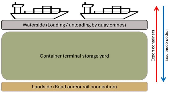
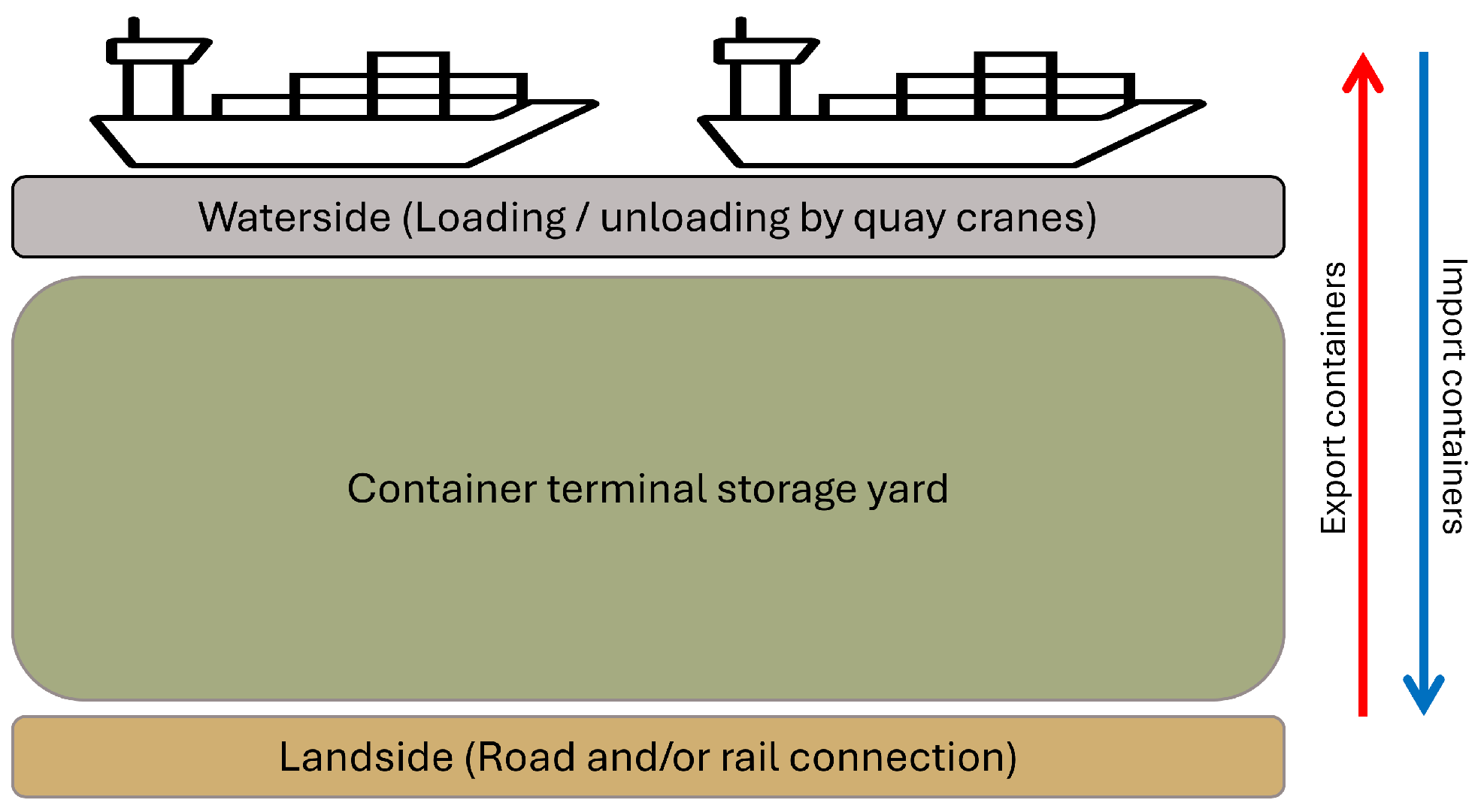
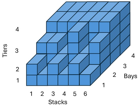
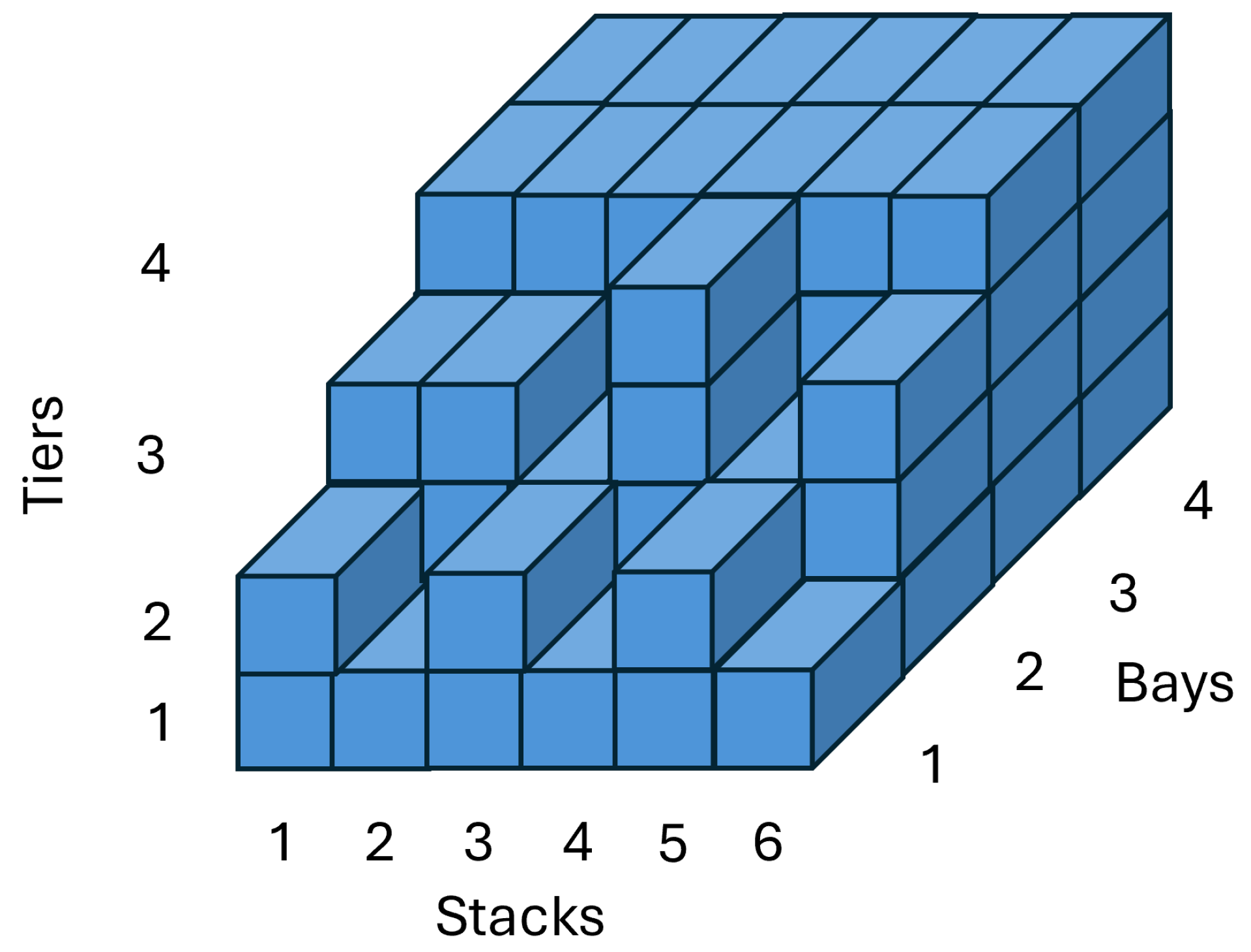
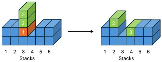
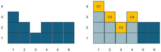
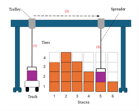
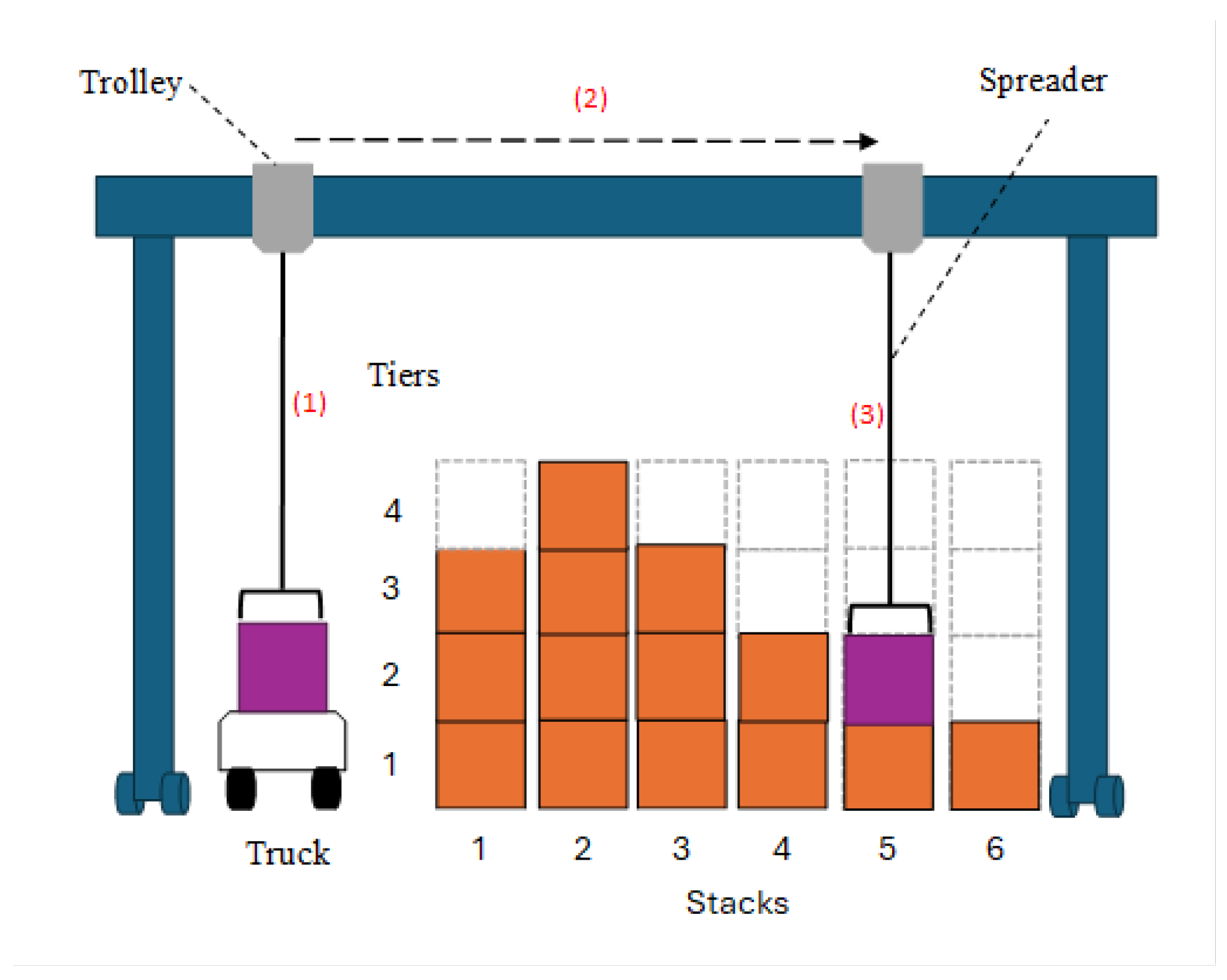
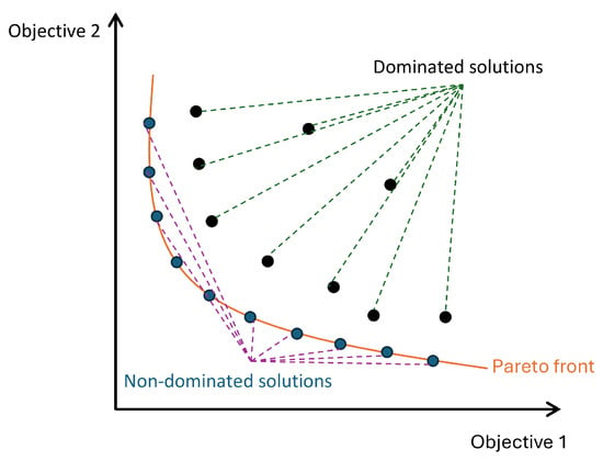
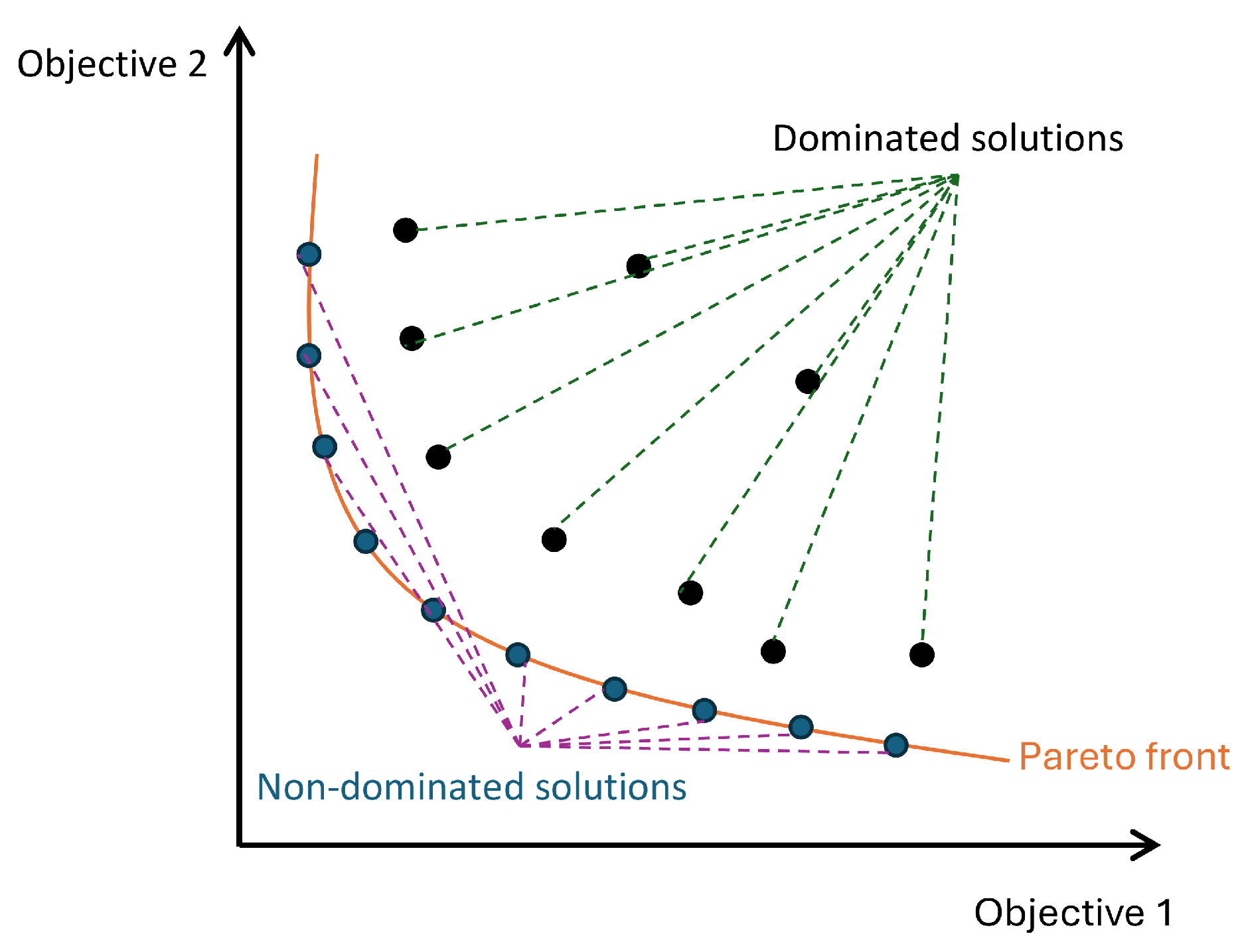


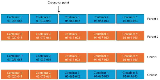
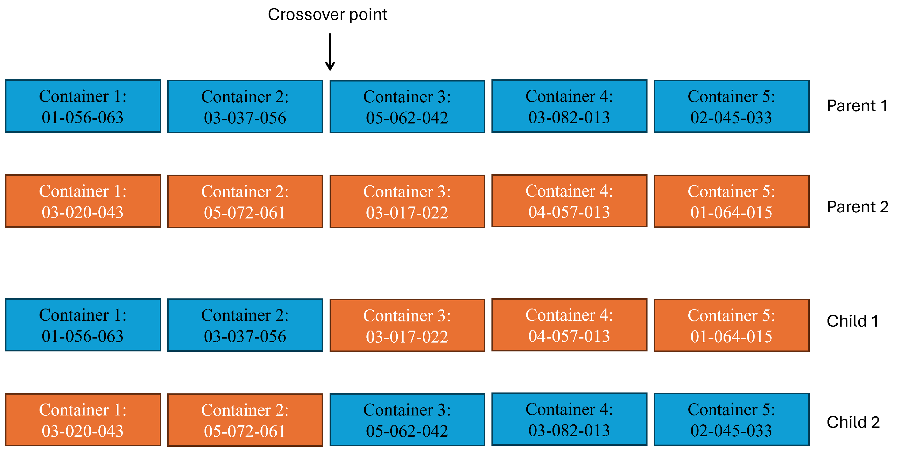
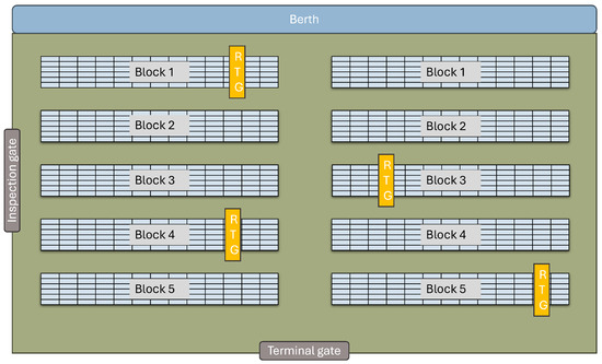
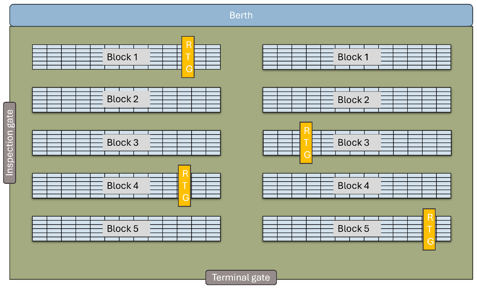
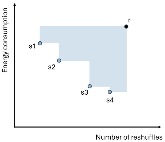
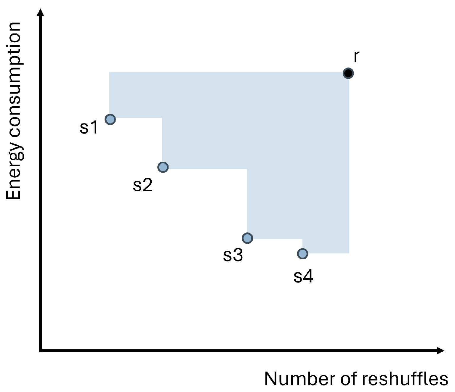
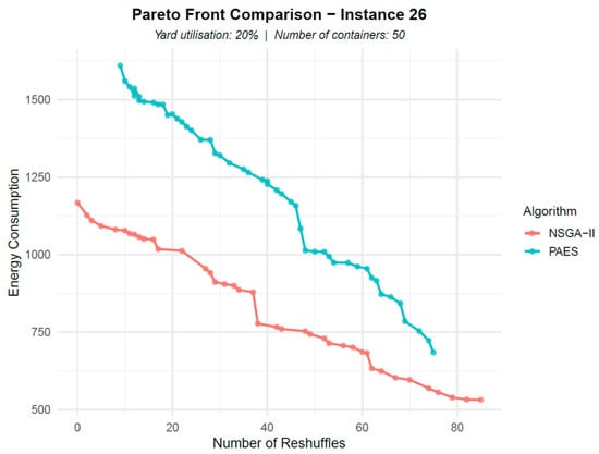
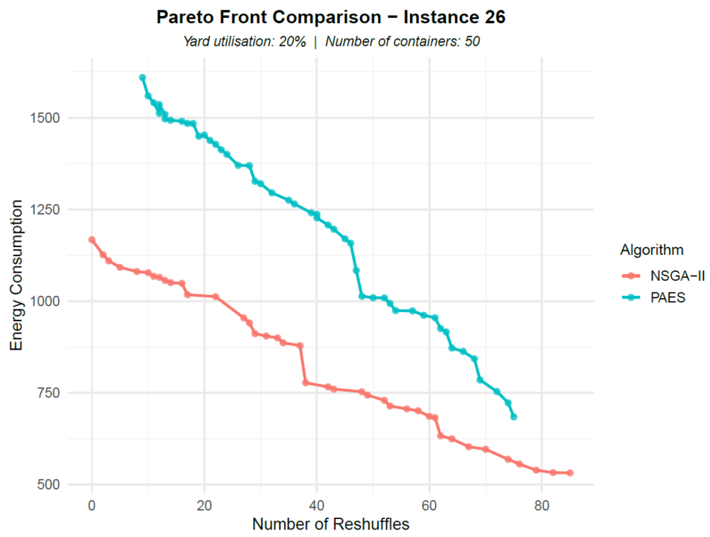
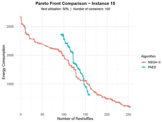
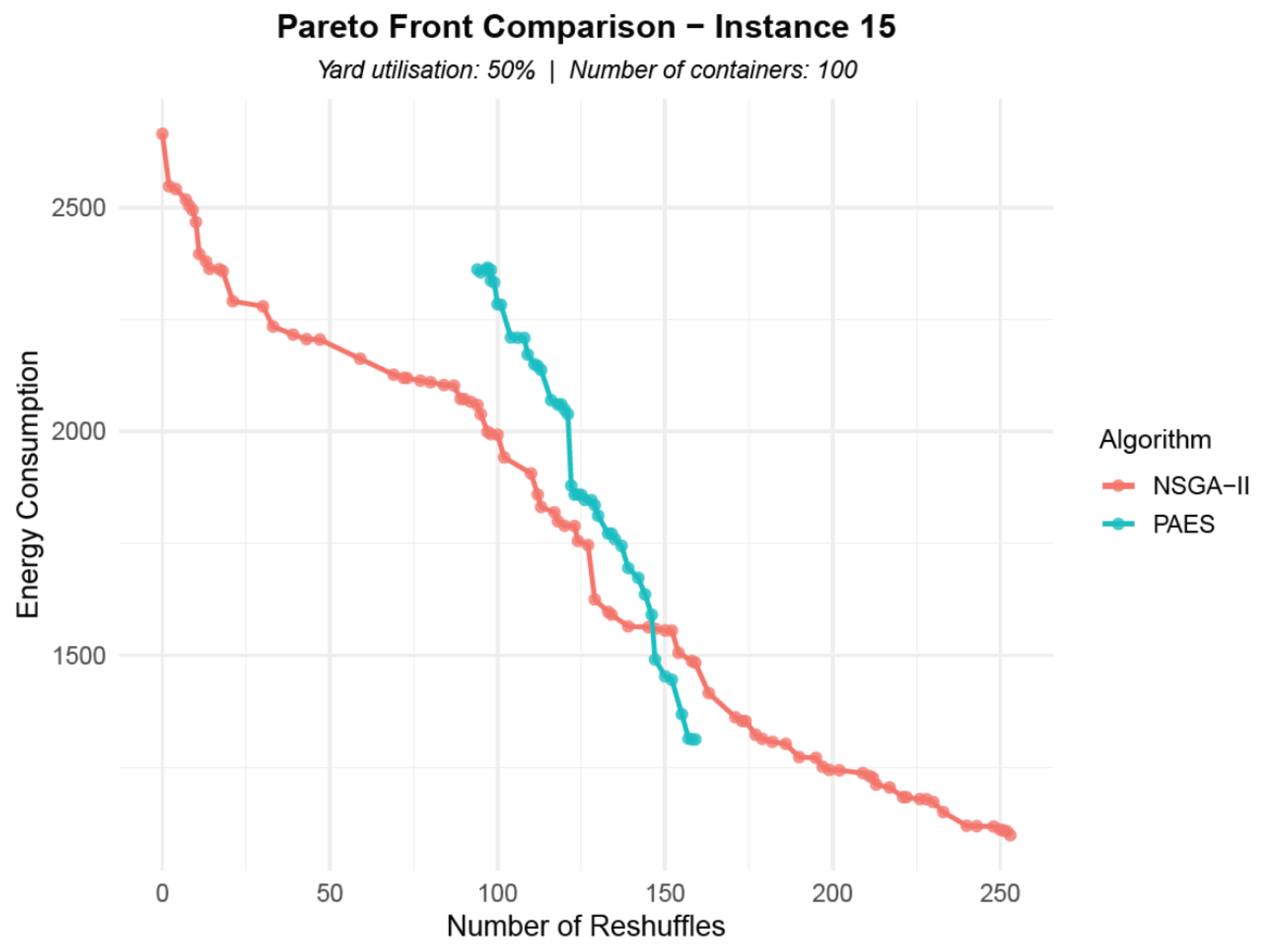
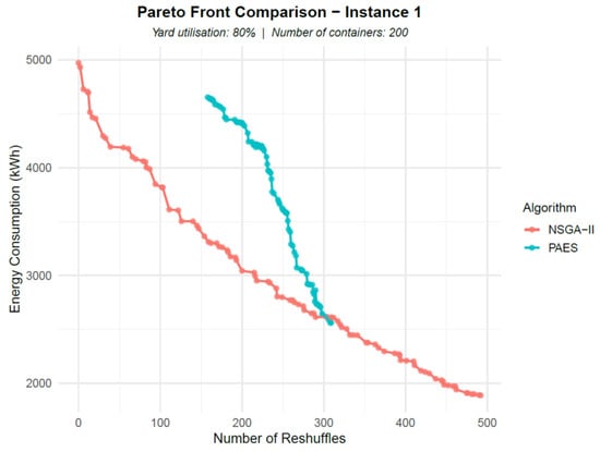
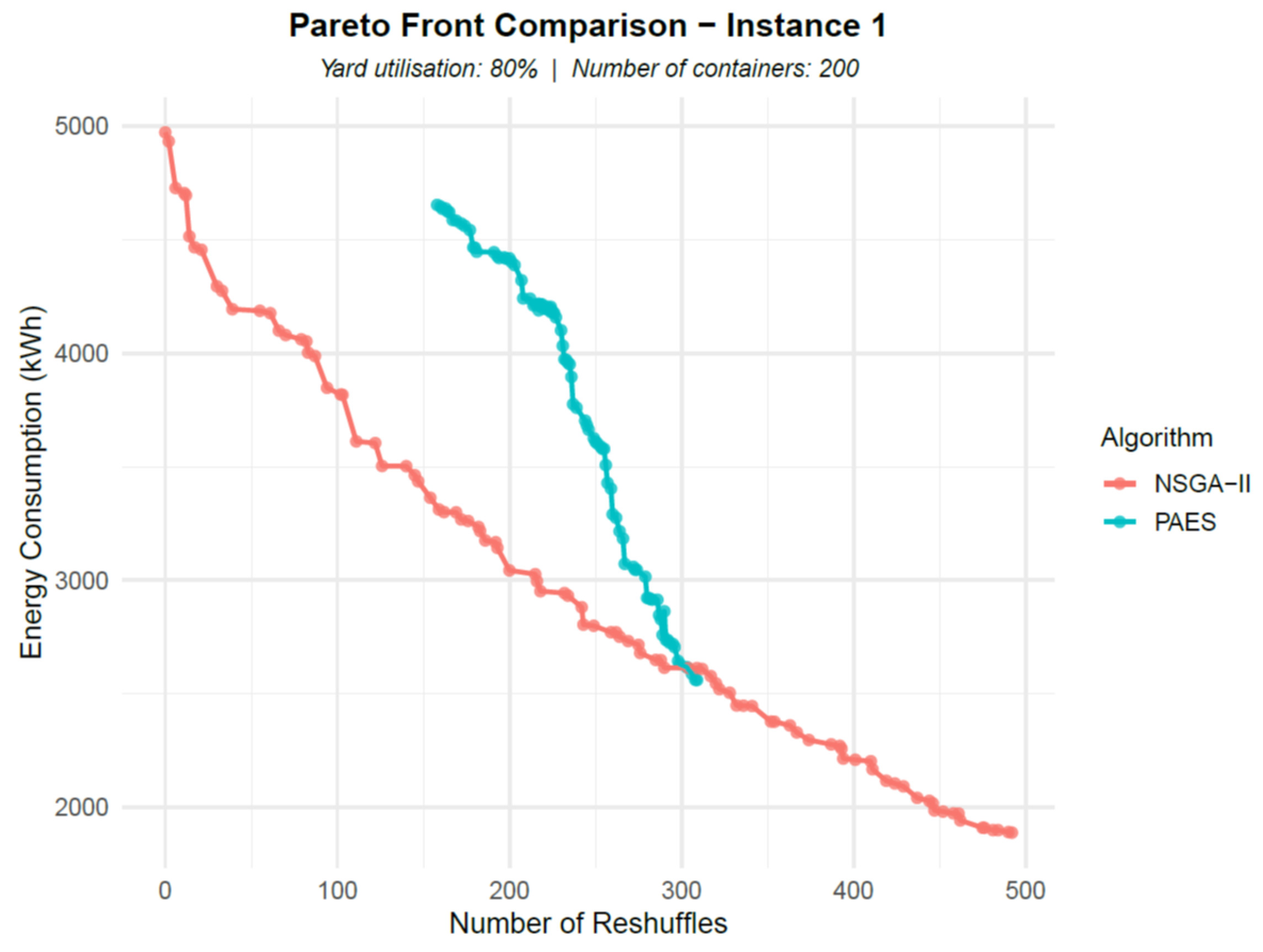
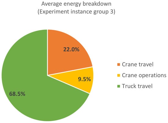
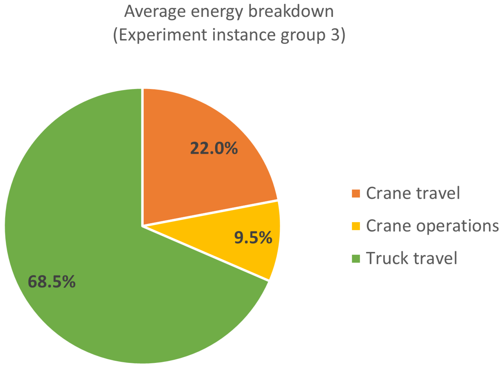
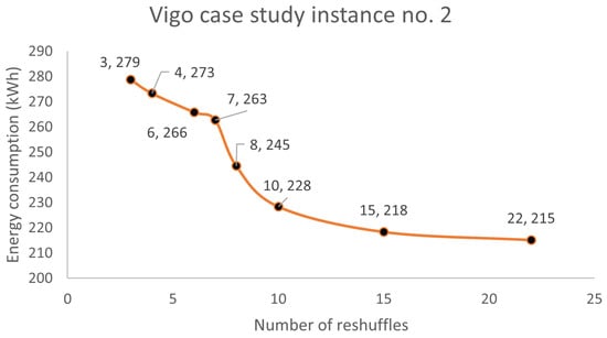
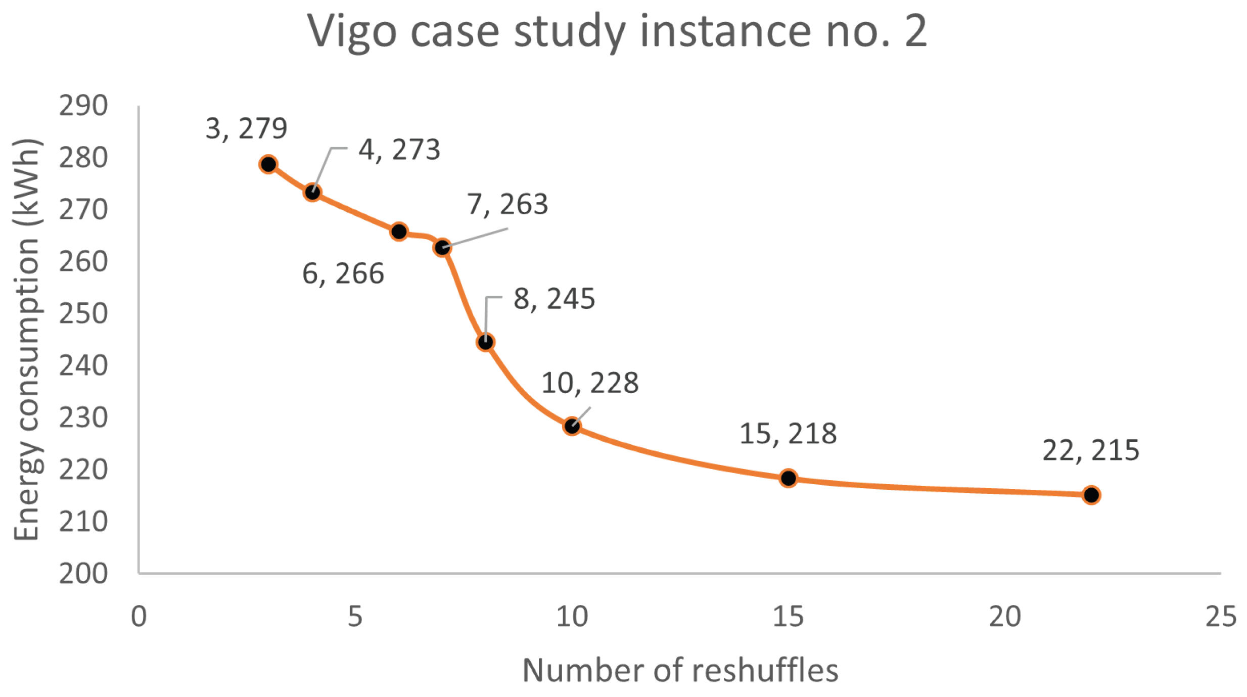

Disclaimer/Publisher’s Note: The statements, opinions and data contained in all publications are solely those of the individual author(s) and contributor(s) and not of MDPI and/or the editor(s). MDPI and/or the editor(s) disclaim responsibility for any injury to people or property resulting from any ideas, methods, instructions or products referred to in the content. |
© 2026 by the authors. Licensee MDPI, Basel, Switzerland. This article is an open access article distributed under the terms and conditions of the Creative Commons Attribution (CC BY) license.