


Abstract
Never has the analysis of bus travel times been so essential to transit planning: travelers complain about a decline in service quality, urban congestion is on the rise, and public transport companies struggle with a structural driver shortage. This research paper aims to address the urgent need to explore new tools to increase commercial speed on transit lines while avoiding costly, potentially inefficient technological investments. A data-driven, cost-neutral, and replicable methodological framework is proposed to provide a first-order estimation of the potential benefits of Transit Signal Priority (TSP) at signalized intersections. The approach is based on Automatic Vehicle Monitoring (AVM) data analysis, which is underpinned by a lean network representation logic built from origin/destination pairs of stops located upstream and downstream of signalized intersections. Bus travel inter-times across network arcs are compared between peak and off-peak periods through a two-level analytical process that progressively refines the estimation of recoverable delay. The methodology is applied to the urban bus network of Pavia (Italy), operated by Autoguidovie S.p.A. (one of the most important Local Public Transport companies in Italy), with a specific focus on the high-frequency PV3 line. Results indicate a potential reduction of up to approximately 6 h and 45 min of operating time per day at the line level (−13.5% of total driving time), and up to 2 min per trip along a 2 km corridor (−6% along the single corridor selected). The procedure integrates both infrastructural and operational perspectives, supporting preliminary decision-making on TSP implementation using only data already collected by transit agencies.
1. Introduction
The Local Public Transport (LPT) sector is one of the key levers for the sustainable development of European cities; it responds to rising urbanization rates, the growing demand for daily mobility, and the need to reduce climate-changing emissions.
Its centrality can be seen from two perspectives. On the one hand, it is worth noting the strategic role LPT plays in ensuring access to services, social equity, and the quality of urban life. On the other hand, considering the workforce it aggregates, the International Association of Public Transport (UITP) [1] reports around 1.3 million workers in Europe employed by public transport (two-thirds of employees are drivers), meaning that in many cities, transport operators are among the largest employers. Thus, the European Union is committed to allocating an increasing share of funds to this sector, recognizing that, in developing public transport, it offers the opportunity to ensure mobility for all while contributing to the achievement of many other common objectives, such as economic development, employment, health, environmental protection, and social cohesion.
However, amid growing investments in support of the sector, public transport is facing a structural crisis that compromises its efficiency and reliability due to multiple, interconnected critical issues. Firstly, there is a chronic shortage of staff, particularly drivers, which directly impacts service deployment and leads to service cancelations and/or reductions, at a time when public transport should be strengthened as the preferred choice for citizens. The growing difficulty in finding new human resources is even more problematic, given that the retirement of the “baby boomer” generation in the coming years will further reduce the available workforce. This picture is also confirmed by some estimates made at the Italian level: ANAV (National Association of Passenger Transport) expects a shortage of about 8000 new drivers in the next three years alone [2]. Furthermore, the Italian Ministry of Transport estimates that 45.8% of drivers with a CQC (Driver Qualification Card) are over 50 years old, while only 18.1% are under 40. Then, in contexts where only mixed-traffic routes are present, without dedicated lanes, operational difficulties arising from road congestion directly affect the performance of surface transit services, which are subject to the same traffic dynamics as private vehicles. This causes the system to struggle to maintain service quality and satisfy passenger expectations, as poor punctuality on transit routes results when policies to increase commercial speed are not considered. In the absence of targeted interventions, there is a risk of a vicious circle (Figure 1): reduced reliability and competitiveness of public transport leads to a change in citizens’ choices, who tend to reduce their use of public transport, rely more on private cars, contribute to increasing congestion, and thus put public transit surface services in even greater difficulty.
Figure 1.
A vicious cycle of problems is tackling transport planning (red dotted arrow).
In such a critical sector, it is not enough to focus solely on new hires or to hope for a linear increase in supply. There is an urgent need to introduce tools to analyze how to maximize efficiency in the existing service and make the best use of available resources.
1.1. Motivation for the Analysis
The urgent need to respond to the crisis the public transport sector is currently experiencing, and the opportunity to leverage technologies already available to mobility companies, must prompt all stakeholders involved to experiment with innovative solutions. This motivates the exploration of advanced management tools that improve operational efficiency without requiring regulatory and transport companies to make unsustainable investments [3,4].
In this sense, commercial speed is the variable that best captures the optimization objectives, being an average passenger travel performance, and a significant index for defining production costs for companies. Its analysis makes it possible to explore through a single aggregate measure the advantages that Public Transport Priority architectures offer in terms of service fluidity across the network, for example, when aligned with Transit Signal Priority (TSP) systems.
In mixed-traffic environments, the interaction between different traffic vehicle types and flow patterns at signalized intersections affects LPT commercial speed, which generally tends to decrease. In this context, TSP systems aim to act as mitigation measures, promising optimized traffic flows and reduced junction crossing times by giving priority to public transport vehicles and preventing them from stopping at traffic lights. This contributes to increasing speed regularity across the entire urban network, ensuring greater punctuality, reduced travel times perceived by users, and a lower number of vehicles required to maintain the same service frequency. It also allows for more efficient staff scheduling and, more generally, an overall benefit in service reliability. Clearly, the effectiveness of TSP systems increases proportionally with their level of deployment across the urban network. The higher the number of sensors installed in the network to measure and share data, the greater the number of vehicles equipped with on-board systems, the greater the overall operational efficiency benefits.
At this point, the impact shifts to the cost of these engineering operations, which is quite substantial. Therefore, it is interesting first to analyze the impact of traffic lights and understand how the mission of waiting time reduction can be an immediate and effective lever to recover productivity and service regularity. Identifying the most problematic bottlenecks in the service network allows transport companies to weigh investments more carefully, without unnecessarily increasing operating costs, and to select in a targeted manner which parts of the network are most disadvantaged by vehicular traffic and therefore potentially most benefited by a future implementation of TSP infrastructure.
For this kind of study, it is essential to have vehicle transit data. In this regard, it is worth noting that transport companies already have most of the data they need simply by providing their transport services. Thanks to Automatic Vehicle Location (AVM) and Automatic Passenger Counting (APC) systems, they can collect large amounts of valuable operational data. When properly featured, this data can serve as a useful and valuable resource for identifying the main bottlenecks in the network and for making an initial estimate of the potential benefits of introducing traffic-light priority systems.
The analysis proposed in this article lies at the intersection of two requirements: the need to address the sector’s crisis with solutions that increase the efficiency and sustainability of the service, and the opportunity to leverage existing data and tools to build assessment models that support decision-making.
1.2. Aim of the Study
This study aims to present a procedure for transport companies and regulatory bodies seeking to rapidly achieve preliminary results from the implementation of traffic-light priority systems in their public transport networks, identifying potential opportunities for technological investment by interpreting the operational impacts of Traffic Signal Priority (TSP) technologies. The objective is not to provide a definitive estimate of their effects, but rather to establish a replicable methodological process capable of quantifying, in a first approximation, the potential margins arising from the application of TSP logic in a generalized surface transport network. The results obtained are intended to support informed investment decisions in these technologies, as well as future studies, simulations, and experimental activities aimed at a more rigorous assessment of their effectiveness.
The entire methodological process and its application have been developed through the coding and implementation of specific scripts in the R-Studio environment. As previously mentioned, the starting point is the aggregation of big data recorded by AVM systems, a data source that transport companies generally have access to. This ensures complete and free replicability of the model, so that companies do not have to purchase transit data from third parties. After a feature engineering phase, input data is aggregated and reshaped to build a simplified model of the service network, with analysis focusing mainly on points where traffic-light-controlled intersections have been identified. At these junctions, the crossing times during the hours of the day when traffic ‘peaks’ are identified are compared with the times of day when traffic is less heavy. Both the identification of peaks and the comparison are performed automatically and dynamically by the model, which ultimately translates this comparison into specific performance indicators and, therefore, into potential service benefits resulting from the adoption of TSP systems at traffic-light intersections in the transport network, to weigh the investment for the transport company on a broader operational scale. The model will then be tested in Italy using recorded transit data from the Pavia urban bus service provided by Autoguidovie S.p.A. company. The paper is organized as follows: Section 2 provides the background of the research; Section 3 presents the proposed method; Section 4 discusses the case study of Pavia, Italy; finally, Section 5 presents the conclusions and possible developments of the work.
2. Background
The results of the analysis of technical and scientific literature, organized into three macro areas as shown in Figure 2, were used to develop the methodological process.
Figure 2.
Tripartition of scientific literature studies reviewed.
2.1. Network Analysis and Policies
A first group of documents collects studies and analyses conducted by research groups and authors seeking common-ground solutions to various critical issues increasingly affecting a sector in difficulty, with users reporting significant declines in service supply. Some studies assert that the perceived quality of public transport offer depends largely on travel time variability, with passengers discouraged by unpredictable journeys or excessive delays compared to scheduled times, especially during peak hours [5,6]. In response, Beria and Battilocchi (2024) [7] consider commercial speed as the primary indicator for monitoring and optimizing performance and quality, as well as for mitigating the adverse effects of driver shortages. This issue impedes the increase in service provision linearly by increasing the resources employed. In view of this necessity, three possibilities of intervention are viable: invest in urban infrastructure solutions, such as priority lanes, to decouple private and public transport traffic; conduct operational measures, such as route design optimization and stop placement redefinition [8]; apply ITS technologies as tools to support strategic planning and to increase the productivity of public transport [9].
Clearly, none of these choices can be made independently from the others: it is essential to promote rigorous processes to analyze the requirements, the feasibility, and the resulting organizational impacts for each of the choices to be implemented [10], without placing excessive emphasis on the positive role of technology, but adequately analyzing user needs and proceeding in accordance with the operational and organizational context of implementation. Among various methods for measuring the impacts of interventions, in [11] the authors introduce the so-called “welfare analysis” and evaluate the effects of introducing dedicated bus lanes on social well-being. Through this methodology, they study the effects of such an urban reset, net of the negative impacts on private vehicle traffic, and conclude that the benefits to bus users outweigh the costs to car drivers, as buses are a much more efficient choice in terms of average occupancy rates. Regarding assessment methods, ref. [12] notes the lack of studies in the literature that address the joint integration of operational efficiency and equity of access, aspects that are optimized separately, and whose interaction has rarely been investigated. For this reason, the authors propose combining Data Envelopment Analysis (DEA) and geographic information systems (GIS) to jointly address efficiency and equity issues.
2.2. Operational Data for Monitoring
A second group of studies focuses on translating general guidelines into concrete, replicable procedures for assessing the feasibility of specific projects in advance. This literature examines in greater depth how transit data—particularly Automatic Vehicle Location (AVL) data—can be used to monitor the performance of urban networks, thereby improving the efficiency of scheduled transport services. This frontier of planning has emerged in response to the need to monitor urban network traffic and, at the same time, to exploit the data that transport companies generate for free. With the widespread adoption of Automatic Vehicle Monitoring (AVM) systems on-board buses and the drastic drop in data storage costs, Public Transit Operators (PTOs) gained access to large volumes of operational data for monitoring the services they provide, with vehicles becoming veritable mobile sensors [13], ‘floating’ within the same scenario to be interpreted and modeled, in constant interaction with ordinary traffic.
Moreover, since the early 2000s, collaborations between organizations (e.g., TriMet in Portland, Oregon [14]) and university research centers have emerged and, together, investigated how to improve service provision to achieve greater efficiency [15]. These collaborations paved the way for subsequent studies demonstrating the benefits of these measures. For example, ref. [13] shows the potential of GTFS Real-Time data for developing a methodology to monitor urban networks. Taking the case of Gainesville (Florida), the authors analyze speeds on road segments within the study area to predict systemic or stochastic delays on segments and to evaluate the punctuality and average speeds of public transport lines. Similar approaches using high-resolution bus GPS data have been applied to identify recurrent delay patterns and congestion sources on urban arterials [16]. Comparing average line-speed charts for the bus service in Portland (Oregon) reveals recurring transit patterns, and delays due to intersections, pedestrian crossings, or stops are explained. By inspecting the most congested areas, the most urgent infrastructure interventions are finally identified, and where it may be necessary to reassess the positioning of stops or create dynamic “queue jump” lanes.
On the other hand, ref. [17] is interesting for the authors’ choice to understand how service variability affects both service planning (timetable construction and vehicle allocation) and the reliability that users associate with it. The basic unit adopted is the terminal-to-terminal bus travel time (from departure to arrival terminal), following the approach described in [18], with AVL (Automatic Vehicle Locator) and AVC (Counter)—AVM subsystems—used as data recorders. The results show a strong temporal correlation between bus and private traffic travel times (comparable daily and weekly trends, with peaks during rush hours) but also highlight high intra-daily variability across time slots. This demonstrates that bus travel times are strongly influenced by the temporal variability of congestion in mixed traffic, confirming the findings of [19].
The choice of [17] to analyze terminal-to-terminal times is in line with what is argued in [18], where the authors debate the fact that most of the analyses in the literature focus on stop-to-stop times. This thesis is supported by several studies on travel time variability and passenger perceptions [20,21,22], and Cats [18] argues that this sacrifices the rarer but more relevant analyses for planners, as they form the basic unit for constructing timetables and service schedules. While recognizing the validity of this observation, an approach based exclusively on the analysis of macro-intervals risks being “blind” to the specific causes of delays and operational variability. Conversely, addressing the problems affecting the arcs between stops enables more explicit, accurate identification of network bottlenecks and quantification of margins for intervention, thereby laying the foundations for targeted strategies to reduce travel times.
A compelling viewpoint is proposed in [23], which our study considers and elaborates on within the following section. In fact, the author chooses to use the same transit data that are also examined to construct the service network, focusing on three main points: locating the areas with the highest traffic rates in the city (network analysis), identifying the reasons behind this, measuring the impact of buses on urban traffic (statistical methods), and developing possible solutions to the problem (simulation). What is interesting in this case is less the result of the study—the author demonstrates that urban bus traffic is not a cause of general urban traffic—and more the method used in the network analysis phase: the network is constructed by choosing bus stops as its nodes, the route between two stops as arcs, and the average time delay between two stops as the weight of the arc. This data is then used to define the importance of each node, measured by betweenness centrality. The basic step chosen to determine the transport network shares the same reasoning as our study. Here, centrality measures are not adopted, as they are less informative for relatively simple network structures, as in the case study of Pavia introduced in the following chapters.
Moreover, this second group includes studies that use AVL data (location and time transits at terminals and stops) and APC data (with boarding/alighting load indices) to calculate, visualize, and compare key indicators of public transport service quality over time. An example is [24], which, to develop an analytical platform with data collected in the Pittsburgh region, focuses on various KPIs such as excess waiting time (EWT), travel time (average/variability), bus bunching, stop skipping, fullness, and on-time performance (OTP). A clear strength of this approach is its ex-post use as a policy tool, as it allows the effects of timetable changes on KPIs (waiting time, punctuality, etc.) to be monitored and corrective measures to be taken. This line of work falls within the established frameworks for measuring operational performance (Transit Performance Measures, TPM) and service quality, as cited in the TCQSM manuals and the TCRP guide dedicated to the construction of performance measurement systems [25,26].
2.3. TSP and Optimization Models
Lastly, a third cluster of studies focuses on methods for aggregating transit data, organizing theoretical models and optimization algorithms to study active and/or adaptive traffic-light priority strategies, and prioritizing public transport to support greater regularity and balance in urban traffic flows. These papers provide the scientific basis for various scenarios and solutions, such as Public Transport Priority (PTP) management [27,28], the use of dedicated dynamic lanes that separate buses from private traffic [29], the study of holding strategies (bus keeping at stops) and speed control (dynamic speed adjustment) to optimize headway regulation and, at the same time, control operational delays, energy consumption, and emissions [30]. Among all the strategies mentioned, the most insightful is the so-called conditional Transit Signal Priority (TSP), a system that has the potential to improve public transport performance and address capacity constraints by prioritizing collective transport movements over other traffic flows [31]. Services for traffic-light intersections are standardized at the European level through the C-ITS framework, coordinated by the C-Roads Platform. The C-ITS framework provides interoperable definitions for traffic-light priority for designated vehicles, including buses. At the same time, the availability of SPaT/MAP information and speed advisories supports smoother operations and reduced stopping at intersections [32].
In line with [31], this study will combine AVM records with TSP activation records to map “where and when” priority is effective, recognizing that the effects of conditional priority are inherently context-dependent and that average corridor results can sometimes mask substantial intersection-specific benefits. Interesting is the authors’ choice to opt for a single-intersection perspective, without aggregating data by transport corridors, through replicable metrics such as delay and recovery. This intersection-level perspective is crucial to highlighting where TSP produces benefits and capturing its context-dependent effects, which are often masked when only corridor-level measures are considered.
For the sake of clarity, it is underlined that the goal of developing a model that is fully accessible and replicable by public transportation companies is also reflected in the choice not to include Signal Phase and Timing (SPaT) data, signal cycle timing logs, on-board brake detection, detailed speed profile analysis, or GPS-based dwell-state detection.
2.4. Main Takeaways and Innovative Contribution
The previous paragraphs show how literature has focused on exploring the resources derived from data from Automatic Vehicle Location (AVL) systems [3,9,33], GPS trajectories [16], and GTFS Real-Time (GTFS-RT) feeds [13]. This means that analyzing models to estimate urban congestion and operational delays accumulated along urban networks can establish a link between the problems that transit agencies face in their day-to-day operations (low service speeds, high variability in transit times, and congestion hotspots at intersections) and some of the main courses of action (TSP technologies and accurate analyses based on complex algorithms). However, these solutions raise further questions.
Firstly, while the use of GTFS-RT as a data analysis tool can improve the accuracy of short-term forecasts and the reliability of service, it involves a significant degree of computational complexity. Its operational use by transit agencies is hindered by the requirement of continuous access to real-time data and rather complex data pipelines, limiting the potential to serve as an ex-ante operational decision-support tool.
Then, the author described the extensive range of studies that utilize historical AVL data or high-resolution GPS data to identify critical congestion points and build models for estimating delays and bottlenecks in bus corridors within operational networks, noting that this often involves descriptive analysis, visualization techniques, or performance dashboards based on KPIs. Although these approaches provide valuable insights into the spatial and temporal distributions of delays, they generally do not focus on aggregating observed delays into metrics of impact on transit service, nor on estimating how specific operational or control strategies, such as Transit Signal Priority (TSP), could potentially help mitigate systemic issues in the sector.
Consequently, this document highlights the significant methodological gap between data-driven congestion identification techniques and readily available, user-friendly tools capable of supporting preliminary investment decisions for public transit priority systems. This void is probably less problematic when collaboration between research centers and transport companies occurs, as in the case cited by TriMet in Portland, Oregon [15], but it widens when collaborative scenarios are absent, and transport companies need internal solutions. Thus, it is important to explore leaner operative tools that can bridge this gap, supporting Public Transport Operators (PTOs) in reaching satisfactory levels of operational efficiency in daily service planning.
Based on the findings of the studies cited above, the work presented in the following paragraphs aims to achieve the following objectives:
- Use AVM data held by transport companies, which can be extracted and used by PTOs at no cost, without the need to invest in new infrastructure or surveys.
- Develop a methodological analysis to evaluate transit data at stops, extract trends in line travel times, and identify misalignments as proxies for urban traffic. Buses are intended as “mobile sensors”, which produce records modeled to track bottlenecks at traffic-light intersections for benchmarking purposes.
- Through analysis, propose a standardized procedure to preliminarily and quantitatively identify the margins for improvement achievable with Public Transport Priority (PTP) systems.
- Provide not only performance indicators (as many studies already do), but a wider ex-ante decision-making screening model that transport companies can use to identify service inefficiencies and work with local authorities to develop an investment plan to improve operational performance, before undertaking more complex traffic simulations or technological field trials.
The newness that fills the methodological gap in the literature lies in the fact that a single tool aims to combine the empirical approach (daily bus operational data) with the evaluative purpose (potential effects of TSP on intersections). In summary, while many studies tend to discuss policy (group 1), monitoring (group 2), or proposing sophisticated TSP models (group 3), this project is innovative because it integrates all these perspectives into a lean, scalable method that can be applied immediately and replicated in other cities at no additional cost. Some of the assumptions made in the following chapters will clearly limit the accuracy and reliability of this empirical approach. However, the simplicity and immediacy of the results from an intermediate, “zero-cost” tool, which can be used as a test before making more costly investments in traffic micro-simulation or infrastructure campaigns, are considered winning factors.
The following methodological framework should be understood as being an operational model, not a theoretical one. Therefore, this study does not aim to introduce a tool that seeks to take the place of more advanced, specific, and precise analysis models, which are already widely covered in the scientific literature. The intention is rather to adopt the perspective of a Public Transport Operator (PTO) and devise a procedure that can be quickly implemented, is easily understandable, and has absolutely no barriers to entry. It is therefore important that the user can understand, use, feed, and sometimes adapt a tool that, if more complex, would be considerably less practical and functional for the purpose for which it is intended.
3. Methodological Framework
The scheme reported in Figure 3 describes the main steps of the model, with the phases of transit data collection, analysis, and integration after AVM systems collection presented below. Specifically, the proposed model is based on four steps: (i) input, (ii) feature engineering, (iii) analysis phase, and (iv) results. After imposing specific spatial and temporal constraints that define the boundaries of the case study, this information is aggregated and reorganized in the feature engineering step.
Figure 3.
Process of analysis scheme: representation of the 4 steps.
A transport network is therefore constructed and serves as a logical twin of the real one, along with a series of KPIs to measure and discuss the impact of applying TSP systems in the operational network. During the analysis, two perspectives are proposed, leading to two levels of complexity, which will be discussed after the application phase in the case study of urban service in Pavia.
The entire process has been developed and tested in the RStudio environment (v2025.09) using about 15 different code scripts, enabling the workflow to be fully adaptable to each application scenario and ensuring complete replicability and rapid applicability through streamlined logic and fast, iterative models.
3.1. Step 1: Input: Dataset Extraction, Preparation, and Normalization
The methodological framework of this study is based on the analysis of transit data collected by the AVM systems of in-service buses. These data describe the “provided” transport service, which is interesting to analyze both independently and in relation to the “scheduled” service, in the GTFS Static format.
The first part of the methodology clarifies how to select and limit data sources to be extracted, analyzed, and aggregated to build the model framework. The perimeter must be delineated in space by circumscribing the analysis area, which includes a portion of the transport network; therefore, by selecting some of its lines to be examined. In this sense, urban areas are preferred for study: greater traffic-light density, more targeted areas of intervention, and higher transit operating frequencies ensure a richer, more robust database. Then, a time constraint must be defined, for which a sufficient extent (greater statistical robustness) but not excessive (more manageable computational performance) is recommended. Furthermore, it is important to assess the homogeneity of the chosen records: they should relate to the same type of service (school/summer) and describe the same kind of day (weekdays/weekends).
The data sources guarantee a comparison between the scheduled service (GTFS Static data) and the service provided and recorded, as described by transit data (AVM/AVL) and load data (APC). Data relating to transit records at bus stops, which form the basis of the entire analysis, are extracted from these two groups.
Attention is paid to the structure of the data in the GTFS Static format, with a detailed examination of the “sub-files” (lists and tables) which define its content. In this case, the core of the entire GTFS Static is represented by the “stop_times” data list, which contains the scheduled transit data for the stops of the whole service network, distinguished by stop code (“stop_id”) and linked to other unique codes that allow this data source to be aggregated with those describing the scheduling of journeys (“calendar_dates”) and their routes (“shapes”, “trips”). Afterwards, “provided” service data, in the form of transit records (AVL) and passenger loads (APC), are introduced in greater detail, and the essential attributes are specified to establish a good aggregation of the scattered data frame.
In both the development of the method and the testing of the algorithms on a specific case study, transit records from the city bus service in Pavia were used, acquired, and stored by the Autoguidovie S.p.A. bus company. In this initial phase, the data covers two months of service and is analyzed only for school-time weekdays (regular service). Once the model is refined, a broader, more diverse statistical base can be analyzed equivalently.
Figure 4 shows how the data appear in this first phase, after the “planned” and “actual” transit data sources are aggregated. The basic unit of the data frame is a transit record described by a couple of important attributes.
Figure 4.
Example of a data frame appearance after extraction. Distance is expressed in kilometers.
- “Route” attributes, information on the line/direction pair (“Line ID” and “Direction”) involved in a particular route (described by the unique code “Trip ID”) and transiting at a specific stop on the network (defined by the “Stop ID” code).
- “Transit” attributes, which associate the information described on the left side of the table with transit information in dd/mm/yyyy hh:mm:ss format. This report includes both what is scheduled by the service (source: GTFS) and what is performed and recorded by the on-board bus systems (source: AVM records).
To adapt operational data to the transport network defined by the scenario and to analyze the performance of the TSP infrastructures to be implemented, a bridge between transit data and the transport network is necessary. This study proposes examining the location of traffic-light intersections in the area and the transit records of buses passing through them. Before, if this information is not available as input, it is necessary to conduct a census of areas with traffic lights, map their locations, and collect their geographic coordinates to enable a direct match with transit records.
3.2. Step 2: Feature Engineering: Logic Network Construction and Basic Attributes Definition
At this stage, each row of the “point-based” dataset corresponds to a single transit record, registered when one of the buses passes through a stop included within the geographical boundaries of the scenario. As a consequence, a leaner logical network is defined to better organize the analysis phase and efficiently aggregate its results.
Starting from the list of network areas where traffic lights are present, all the possible “turns” of each intersection area are identified: this expands the list of intersection nodes to a larger table of potential traffic-light-controlled “maneuvers”. Each of these is linked to a pair of origin/destination points, described in the network by a set of bus stops (Stop IDs). More precisely, it must be identified for each “maneuver” an observing point downstream of the intersection (origin, “stop_in”) and one upstream (destination, “stop_out”), each of those referred to a particular GTFS “Stop ID”.
Through this transition tool, a scattered, point-based transit dataset is transformed into aggregated, arc-based transit information that describes bus behavior across traffic-lighted junctions.
For ease of understanding, Figure 5 presents an example of how the list of “maneuvers” is constructed, to be used as above in the transition from a “point” to an “arc” based network. The specific case includes a fragment of the list corresponding to the “maneuver” with unique code 81, which is part of the set of turns at the traffic-light intersection located in the “Riviera/Adda” area. This example and each of the other “maneuvers” require two lines describing the observation points upstream (“stop_in”) and downstream (“stop_out”) of the traffic-light intersection, each linked to a “Stop_ID” code. Once the correctness of the information has been verified, this code transforms the pair of disaggregated transits recorded by the AVM systems via the “Stop_ID” code equal to “PAV292” and “PAV229” into a single transit at the “maneuver” arc 81 in the “Riviera/Adda” area.
Figure 5.
Portion of “maneuvers” table.
To make more complete and realistic use of the list of “maneuvers” defined for each traffic-light intersection, it is necessary to integrate additional network-based input. In fact, TSP systems underlie the need for new management tools to control the assignment of virtual priority corridors.
- The simplest scenario assumes these corridors are always independent within the service network, with no intersections between them.
- However, actual conditions make it necessary to consider in advance how to manage multiple-priority calls converging in the same area.
Because of this, the study’s methodology integrates an “adjacency matrix”. This 0/1 binary matrix is used to define network links, indicating which vertices are connected by existing arcs, and contains
- as its indices, both on the rows () and columns (), the codes which are univocally assigned to each of the turns (“maneuvers”);
- within its cells (), a value defined by the condition in Equation (1).
The matrix is here filled manually by checking the adjacency conditions of all turns and intersection areas. For each turning point index, it contains in its rows (symmetrically, in its columns) a vector of values in case of non-conflicting turns (), or otherwise. Thus, it is possible to quickly define, for each -th turning index (row vector), the turns which are non-adjacent with respect to i, extracting the positions where zero values are. As a result, it is possible to extract the maneuvers generating conflicts in TSP systems with closely spaced priority calls within a given network corridor.
After clarifying how to prepare all the data sources taken as input for the methodology, the aggregation steps based on the temporal transit information are presented below. The study uses the dataset structure shown in Figure 4, with particular attention to the “Actual Transits” column.
First, for each “maneuver” included in the list of traffic-light intersections, the “crossing inter-time” is calculated. The stop-based transits for the list of ‘maneuvers’ are transformed into transit inter-times, notably by date (day/month/hour of transit), “Trip ID”, “Line”, and “Direction”. Each is calculated as the time difference between the transit detection at the point of origin and that at the point of destination. This is done both for the programmed transits (benchmark) and the actual transit data (comparison).
Then, cases with marked or inconsistent mismatches between scheduled and actual transits are filtered out. This is done according to the time slot in which the mismatch occurs, since the “crossing inter-time” is expected to be higher when the time slot is comparable to a period of the day when generalized traffic peaks.
Thereafter, a strategy is established to quickly transform these transit times at traffic-light intersections into performance indicators for TSP systems intended to support public transport operations. A literature review shows that some studies do not go beyond comparing the transit times (i.e., the intervals) “predicted” by timetables with the actual times recorded by AVM systems [3,9]. Although this approach is straightforward to implement, it fails to provide meaningful results. In fact, such a comparison would not give an overview of the points most affected by generalized traffic, but rather information on the alignment of timetables and actual service performance (reflecting only the accuracy and quality of the information communicated to users).
Instead, this paper proposes an innovative perspective, measuring a proxy for the effects of TSP infrastructure at traffic-light intersections in the transport network, focusing on “actual” transits, and comparing “crossing inter-times” during ‘peak’ and ‘off-peak’ traffic periods.
It is important to underline the methodological nature of the “gap-time” variable introduced in this study. This parameter is not intended to represent a theoretical breakdown of intersection delay, such as control delay, queue delay, or signal delay. Such examples would require detailed information on signal timing, approaching traffic flows, queue lengths, and the multimodal composition of traffic. Moreover, that data is generally not available to public transport operators (PTOs), whose only systematically accessible source consists of AVM/AVL transit logs. Consequently, classical formulations of delay cannot be reproduced within the scope of this study’s data.
Because of this, “gap-time” is formulated as an operational proxy that uses bus trajectories as “mobile sensors” and captures the systematic difference between interaction times observed during peak and off-peak traffic conditions. Since the same maneuver requires a longer transit time under congested conditions, the resulting time difference provides a reproducible estimate of traffic-related delays that could theoretically be mitigated through the implementation of Transit Signal Priority (TSP) systems. This pragmatic approach aligns with the methodology’s purpose: to provide a low-cost, replicable, first-level assessment tool that PTOs can apply independently using only the data they already own, before undertaking more complex or data-intensive analyses.
The basic variable of the analyses presented in the following paragraphs is called “gap-time” and is defined in Equation (3).
where is calculated as the difference, for the same transit made by the same line/direction combination at the same maneuver (i), between a “inter-time” measurement taken in ‘peak’ () and ‘off-peak’ () traffic conditions.
For a proper definition of , it is essential to determine how to identify traffic peak periods using the available data. The most immediate method combines the transit registration time with a “peak flag” (TRUE or FALSE). In simple terms, this can be done “statically”, by referring to pre-established time slots commonly adopted in operational practice or based on scientific literature outcomes. However, a different approach is taken here, and peak periods are identified using dynamic, automatic logic, cross-validated for each case study in which the methodology is intended to be replicated.
The transit data is used directly to identify on the network where traffic congestion is most critical and thus estimate the benefits that TSP systems can bring to the line service. Firstly, it entails determining the daily time periods during which AVM systems systematically record transit slowdowns comparable to those observed during peak traffic conditions. Then, for each trip/direction of travel, the actual commercial speed is estimated from AVM transits as the weighted median of segment speeds, calculated between consecutive stops and weighted by segment length. Subsequently, each trip is associated with a discrete time slot (with 15′ intervals within the 05:00–22:00 service window) based on its start time. For each direction of travel, the commercial speed trend is then analyzed using a time-smoothing procedure to mitigate the punctual variability of individual transits.
The comparison of aggregated commercial speed after smoothing across all daily time slots is used to set a dynamic speed threshold for automatically classifying “peak” and “out-of-peak” time windows. By definition, a systematic reduction in commercial speed compared to average daily behavior is associated with peak conditions (Figure 6).
Figure 6.
Commercial speed by time (red bands = ‘peak’ of traffic time windows).
The graph in Figure 6 shows the average commercial speed data recorded for routes traveling uphill and downhill over the course of an average day of service. For each route and direction, the commercial speed data (y-axis) was averaged, and depending on the departure time of the trip, this information was linked to a specific time of day (x-axis). This was done every 15 min (which is why there are 4 vertical bands of data points per hour). The blue line represents a LOESS (Locally Estimated Scatterplot Smoothing) curve highlighting the average evolution of the average speed of the line corridors throughout the day. Notice how this commercial speed trend band “drops” during periods of increased traffic. For greater evidence, these time slots are highlighted with an orange background, and the points are colored red during periods of the lowest average commercial speed.
The result of the process is the assignment of a binary indicator (peak/off-peak) to each time slot of the day, which is then propagated to the entire transit dataset. This distinction serves as the basis for subsequent analyses, allowing a structured comparison of service performance under normal operating conditions and under increased congestion, and for estimating the potential benefits associated with traffic-light priority strategies.
3.3. Step 3: Analysis Phase: Multilevel Analysis of Time Losses
For the forthcoming steps, the “gap-time” associated with each turn, line, or direction is interpreted as a theoretical recoverable time (only during the “peak” of traffic, see Equation (3)) under the assumption of “ideal” traffic-light control for LPT. In the best-case scenario, peak conditions would behave like smooth conditions: no significant queues at traffic lights, reduced bottlenecks, and alignment of actual times with those observed in non-congested conditions. In this context, the “gap-time” provides an upper bound of the recoverable time within traffic-light junctions.
The set of tables shown below in Figure 7 highlights the aggregation steps the initial transit dataset must undertake to reach a condition that supports a correct analysis of the benefits of implementing TSP architectures (the last table in Figure 7).
Figure 7.
Three steps of aggregation undertaken by the dataset.
With the data available to present, it is possible to quantify the time lost on a typical operational day at individual traffic-light junctions during peak hours, for each maneuver and in each combination of line and direction. Two simulation scenarios are presented:
- In the 1st level analysis, the methodological path follows the assumption of total line preference on all the traffic-light-controlled intersections they pass across;
- Instead, the 2nd level replicates a more realistic scenario, observing the effects of priority systems in a limited area restricted to sequences of three intersections.
3.3.1. First Level of Analysis
The first perspective assumes complete transit priority for all bus lines and at all traffic-light intersections within the study area to estimate the upper limit of the benefits a TSP system provides to daily operational service. The individual “gap-times” are aggregated by “Trip ID” (sequence of maneuvers for each line/direction), and added together to define a new line attribute, defined as “gap-time sum” or T(gap) according to Equation (4).
Now, it is possible to directly measure how the T(gap) value can serve as a proxy for estimating the TSP benefit at the end of a typical day of service. However, it is necessary to first introduce data describing average travel time for the line/direction pair (calculated from transit data) to enrich the mere analysis of traffic-light priority benefits in terms of time saved, by considering also their relationship to each line/direction’s actual travel time.
Equation (5) considers as the ratio between the number of trips recorded during “peak” time slots with respect to the total of trips per day, a factor that extracts only the fraction of trips made during “peak” traffic time bands, thus, that benefit from traffic-light prioritization. According to the off-peak-relative gap-time logic established, journeys made during off-peak hours would not have any operational advantages. They should not be considered as part of the lost (recoverable through TSP) time.
is a proxy of the total time for each line/direction pair at traffic-light crossings and a measure of time possible to be “recovered,” raising operational efficiency; thus, its meaning is twofold.
- Wanting to improve service levels for users means adding more journeys per day while keeping the same number of drivers and vehicles (fixed costs), thereby increasing service frequency during peak traffic (and bus load) time slots.
- Otherwise, to contain service costs while maintaining the same level of service offered to users, this variable could be seen as the time saved from the operating schedule (Equation (6)), with an appropriate distribution of shifts (by excluding the denominator in the equation). This immediately translates into lower variable costs (the same driver for the same service to users makes shorter journeys, with the same routes and frequencies) and, in the best cases, also into lower fixed costs (the possibility of using fewer vehicles or drivers for the same tasks).
At the end of this first part, the two equations presented (Equations (5) and (6)) are applied to every route/direction in daily service. The output (expressed in time units or equivalent shifts) reflects the benefits of LPT priority strategies at traffic-lit junctions along the urban corridors they intersect. This allows the design of the “maximum priority corridor”, intended as the line path that provides the greatest TSP-related benefits when prioritized.
Consequently, for a correct priority management when different “maneuvers” may interfere during the same green phases, it is necessary to introduce a simplified application of the “adjacency matrix” presented in Section 3.2. Starting from the “highest-priority corridor,” the impact that its priority has on other bus routes is calculated using the definition in Equation (7). Its definition determines the attributes T(gap) considered for all route/direction combinations, net of the total preference toward the maximum benefit route.
Equation (7) starts from T(gap) defined in Equation (6), and subtracts two terms, representing:
- The first one defines the “gain” associated with each of the non-adjacent turns, which, by losing priority, loses its “gap-time” benefit, too.
- The second term captures the time redistribution among conflicting maneuvers, assuming perfect conservation of total transit time within the same intersection.
This new equation provides an opportunity to “correct” the contribution of T(gap) relative to the perceived benefits of the highest-priority approach, thereby obtaining a perspective closer to the operational reality of the benefits associated with a complete conversion of the urban network to LPT prioritization.
Even though this pipeline can set an upper limit on performance achievable with a complete infrastructure, it falls short in terms of real economic investment efficiency, with poor operational returns on monetary and time expenditures. This motivates the additional step of analysis, which is introduced and presented in the following paragraph.
3.3.2. Second Level of Analysis
The second level of analysis aims to define a result that describes a more realistic infrastructure situation, so as to analyze the network subsections more strategically. There is no assumption of complete priority for all lines and directions covered by the scheduled service. Still, there is an intention to narrow the analysis, targeting the network’s most inefficient points and focusing on them. This effort is motivated by findings in the literature that strongly link the variability of bus travel times to local dynamics and specific urban nodes or corridors [16,17]. Efficiency-seeking can be practically translated into a minimization problem for hardware to be installed both on board the vehicle (On-Board Unit, OBU) and near the traffic-light intersection (Road-Side Unit, RSU).
Methodologically, the study identifies multi-arc sections linked to the most significant accumulations of “gap time”, allowing for a more target-oriented, while still aggregated, selection of the most problematic service branches, and isolates them in a precise and intuitive way within the urban network. For each line/direction combination, the algorithm is designed to extract the multi-arc triplet i→j→k associated with the maximum sum of “gap-time”, accumulated when crossing traffic-lighted junctions in three adjacent and consecutive areas. The results are reported in a table and plotted on a Leaflet map.
A maximum 2 km distance defines the size limit beyond which the triplet of points is excluded. This “spatial constraint” ensures that the three turns considered form a single “operational block” and circumscribes a compact section of the network where the same vehicle can accumulate close, homogeneous delays.
- This boundary ensures efficient forecasting of traffic-light priority systems, guaranteeing coordinated implementation with minimal infrastructure costs.
- The methodology remains consistent with the literature, which emphasizes the need to assess effects on urban corridors or clusters of adjacent intersections rather than overly extended segments [27,31].
Once this step is performed, for each line/direction pair, the list of transits is sorted in the same sequence as the stops along the route. In this way, each line/direction pair becomes an ordered sequence of turns that can be linked in successive triplets of i→j→k maneuvers, with two strong control constraints:
- The distance covered from the start of the “Trip ID” until each of the detection points () must be lower than the distance covered to reach the following point of the triplet (sequence consistency check);
- No other stops () whose entry distance is between and (sequence density check) are present.
As soon as a valid triplet of maneuvers is found in the line/verse pair,
- The sum of the “gap-times” accumulated over the three arcs becomes the weight of the multi-arc defined by the triplet;
- The distance between the first and last observation point, which must comply with the maximum distance constraint, is calculated.
This process continues until the -th “Stop ID” value of the multi-arc triplet equals the index of the one describing the last maneuver of the previous line/direction. Hence, the triplet of arcs with the maximum weight (“gap-time”) is extracted, and the process is replicated likewise for all line/direction pairs.
By mapping these results, a set of 10 (limit value imposed at the outset) segment sequences is displayed, chosen, and sorted by time “weight” value. This result allows intuitive identification of network hotspots where travel delays accumulate during peak hours, as well as a numerical description of these hotspots (by sequence length, maneuver, and total “gap-time”). Furthermore, it bridges the gap between statistical results and practical convenience, showing where it is worthwhile investing in a TSP infrastructure setup, providing a first approximation of the expected operational results (Figure 8).
Figure 8.
Three multi-line arcs between Partigiani street and Gorizia street (line PV3).
3.4. Step 4: Results: Analysis Results Implementation
The reallocation of any time “recovered” from the schedule through preferential strategies can be treated in the same way for both analysis strategies. Since the transport sector struggles to guarantee the level of service established by contract, the time fraction “saved,” measured as a TSP-related benefit, is assumed to be used to ensure a more reliable service, without changing scheduling or adopting a “thicker” timetabling.
In terms of planning, the results can be achieved in just a few steps:
- First, set the investment size to be undertaken relative to the benefits promised by TSP infrastructure (i.e., the number of OBUs and RSUs to be installed).
- After deciding “what” and “where” to prioritize, whether a line, a route, or just an intersection, the total “gap-times” benefits linked to the prioritized unit are computed, as well as the additional times linked to collateral “non-adjacencies”.
- For all the line/direction combinations, the total “gap-time” is the value to be subtracted from the average journey time of the line in question, in each of its “segments” present in the “block” of the scheduled drive shift (called “tape”).
- A new version of the “post-intervention” operating scenario can now be simulated, accounting for reduced journey times on lines that benefit from the direct effects of TSP strategies.
- At this point, by calculating the driving and working time for each driving shift, it is possible to measure the economic return resulting from the efficiency delta in the service and, by comparing it with the fixed and operating costs associated with the preferential treatment, to assess its long-term cost-effectiveness.
4. Case Study: Autoguidovie Urban Bus Service in Pavia—Italy
The paragraph presents the results of applying the methodology to the urban transport service in Pavia (Italy), operated by Autoguidovie S.p.A. company.
Pavia is a city located in the south-west of the Lombardy region, about 35 km south of Milan. It covers approximately 62 km2 and has a population of around 71,646.
Autoguidovie S.p.A. is one of the most important Local Public Transport companies in Italy. The company provides transport services across various regions of northern Italy, primarily in Lombardy, Emilia-Romagna, Veneto, and Piedmont. Autoguidovie and its controlled companies manage a fleet of over 1500 buses.
4.1. General Results
The case study covered 11 urban bus lines operating within the municipality of Pavia and in some rural areas immediately adjacent to it, generating approximately 2.4 million transit data points during the first two months of the winter school service, from 7 January to 7 March 2025. The geographical area circumscribes the observation to 47 traffic-light junctions (out of a total of 82 censused), whose transits are recorded into a simplified network of 163 origin/destination “maneuvers”, distributed along a monocentric urban network organized around the city center and two mobility hubs of interchange: the bus and the railway stations, both not far from the center.
Figure 9 illustrates a part of the bus network, which has the strongest line forces:
Figure 9.
Representation of the main bus lines in Pavia LPT network. Focus on the central part of the network, with railway and bus station highlighted. Each dot is a traffic-lighted junction.
- PV3 line (E-W axis, highest frequency route) and PV1 line (N-S connection).
- PV4 and PV6 lines (Northwest quadrant).
Almost all the traffic-light intersections in the survey are crossed by these five main lines, making it strategic to study their time lost at traffic lights.
The peak of the traffic detection algorithm described in Section 3.3 and in Figure 6 highlights two time-windows with observations of traffic “peaks”: one in the morning (07:15–09:15) and one in the afternoon (16:15–18:30), consistent with students’ and workers’ daily routine and their time of arrival/departure to their destinations.
Concerning the basic variables, the distribution of values for the “gap-time” attribute across the maneuvers (key: maneuver code) is shown above in Figure 10. As the distribution of “gap-time” values shows, the median “delay” during peak hours is around 15 s (its position is marked by the dashed red line). Over the 153 maneuvers that are part of the 5–95° percentile, approximately 50% of maneuver records show a “delay” of <10 s, around 22.5% have values between 10 and 20 s, and 16% have a “gap-time” of >30 s. Few but insightful cases record time delta values around 60 s.
Figure 10.
Gap-time spread (5–95° percentile) over the maneuvers (“delay” frequency plot). The dashed red line indicates the median “gap-time” measured across the traffic-light-regulated crossings.
The runtime of the analysis algorithm described in the methodology is detailed below, with the operations broken down by five consecutive steps.
- Data preprocessing and filtering take approximately 10 min in total. This time is required to acquire the three types of input presented: static GTFS data (≈1.57 million rows), APC passenger records (≈1.43 million rows), and AVL transit logs (≈2.34 million rows). Merging the three sources produces approximately 1.57 million matched records, entirely related to the city bus service. Only perfect matches between GTFS and AVL are retained, while discrepancies with APC generate NaN entries. Finally, only observations related to weekdays are extracted (1.1 million records, describing 44 service days), and only transit trips associated with mapped signalized intersections are filtered (approximately 847,000 records).
- The dynamic identification of peak and off-peak hours takes about 1 min. The 847,000 observations acquired previously are used as input and serve as the basis for classifying traffic into “peak” and “off-peak” intervals, using an assessment of the commercial speed trends of the lines at 5 min intervals.
- Next, the “maneuver-based” logic is applied to the transit data, in a process that takes approximately 4 min in total. This phase enables the transition from a node-based network (based on stop nodes) to an arc-based network (based on trips). All valid O/D transit pairs are extracted, the basic attributes (time interval, passenger load, line/direction, segment distance) are calculated, and the list of unused maneuvers for each intersection is verified. This results in a dataset that is then used to calculate “gap-times,” a process requiring approximately 45 s and generating the primary variable used in the multilevel analysis.
- The first-level aggregation takes about 10 s, necessary to identify the priority corridor with maximum benefit, apply the adjacency matrix logic, and estimate the potential operational benefits for the PTO.
- Finally, there is the second-level analysis, which takes about 5 s to reorganize the dataset and extract local delay clusters. For each line/direction, three maneuver sequences (triplets) are constructed; the triplets with the maximum cumulative interval time are selected and mapped onto the network.
The entire workflow runs in just a few minutes when applied to a medium-sized urban network with millions of AVL/APC/GTFS records. This confirms the replicability and computational efficiency of the proposed method, even when applied to larger and more complex networks.
4.2. First Level of Analysis Results
Assuming total prioritization of traffic-lighted intersections over transit lines in the transport network, the first level of analysis clearly shows that the critical corridor is the one traveled by line PV3 (the east–west urban bus corridor).
- In terms of “total gap-time sum”, this route accumulates approximately 4–5 min per run (depending on the direction), quantifying the potential benefits of whole-route TSP application: a reduction of approximately 30% in the total time of each scheduled trip. In terms of service planning, it is the corridor with the highest frequency in the network; thus, it is the one where the benefits of TSP technologies are spread more effectively during daily service.
- Surprisingly, the north–south route covered by line PV1 (a long, frequent route) shows a rather marked imbalance in delays at traffic lights during peak traffic hours. Prioritization impacts should therefore be analyzed in greater detail.
- Lower benefits but higher frequencies are associated with lines PV4 and PV6.
- Good potential benefits are also estimated for lines PV22 and PV23, whose effects are affected by the lower planned frequencies.
The high benefit value associated with line PV3 makes it the so-called “maximum priority corridor” to favor when considering traffic-light junction crossings (13 in total).
Therefore, it defines the benchmark for tracing the conditions of “adjacency” and conflict, considering the directions taken at intersections by PV3 line different route trips. For that reason, the operational effects of the full implementation of TSP systems are estimated using Equation (6), which excludes the presence of conflicting “maneuvers” that interfere with the main corridor. On all other routes, the “total gap times” are calculated net of the impacts of maneuvers interfering with the main preferred route using Equation (7).
4.3. Second Level of Analysis Results
Changing perspective, the second level of analysis identifies the “triplets” of consecutive arcs associated with the maximum accumulation of “gap-time”. Results seem to confirm what has already emerged from the first perspective; however, the deeper perspective offered by this analysis highlights the most impactful corridors, where the lines incur the greatest losses due to traffic delays. Once again, the possibility of implementing TSP systems on the PV3 line corridor promises a good operating margin: the analysis quantifies, during peak hours, a median increase in transit times of approximately 1′30″ per trip in each direction along segments of about 1.5 km length.
Unlike the previous case, by focusing on individual network segments (ignoring the impact of bus line frequencies on arcs), this second-level analysis reveals portions of the network that affect lines of “minor” operational importance, even though they pass through vital urban arteries. Specifically, lines PV22 and PV23 are highlighted, revealing localized losses that are potentially even higher than those of line PV3 (approximately 2′00″–2′30″), which instead accumulates more scattered fractions of “delay” along its entire route and suffers only a greater overall slowdown.
The major output of the analysis is reported in Figure 11, where a portion of Pavia’s urban transit network is plotted, with 10 multi-arc triplets, each associated with its respective line/direction pair and identified by a distinct color, as indicated in the legend. This map fragment highlights where higher “gap-time” values are concentrated, and it is obtained following the multi-arc triplet modeling process. The algorithm described above calculates the “gap-time” values for all line/direction pairs in the service network; subsequently, for each pair, it extracts the triplet with the highest “gap-time” value. Finally, using the information contained in the ‘shapes’ files of the GTFS dataset, it reconstructs the corresponding line routes and plots the elements identified by the analysis on a map.
Figure 11.
Second-level analysis results, leaflet map of the top 10 triplets by multi-arc “gap-time”.
At the network scale, the results of this second analysis clearly indicate that the primary source of recurrent delays in the Pavia transit system is the beltway surrounding the city center. The highest “gap-time” values systematically concentrate along this orbital corridor, particularly on the segments corresponding to Viale Lungoticino Visconti and Viale della Libertà (line PV21), Viale Cesare Battisti (PV3), Viale Matteotti (PV3, PV4, and PV23), Piazza E. Filiberto, and Viale Gorizia (PV3).
5. Conclusions and Further Development
The study of operational inefficiencies in the service network is one of the most important tasks for service planning departments and, more generally, for transport companies. Locating delays, investigating their causes, and proposing infrastructure schemes to improve traffic flow in transit networks are major focuses of the scientific literature on these topics. This is because the result can only benefit all those involved in mobility, with increased commercial speed guaranteed by a smoother service and more regular transit.
Reducing delays benefits transport companies: operating costs get reduced, driving duty scheduling becomes simpler and more profitable with the same workforce. This results in less driving time for drivers, since required driving time is lower and remuneration is potentially higher for the same number of kilometers traveled, and a more economical service for companies, with lower fuel costs and vehicles engaged for less time.
Reducing delays benefits passengers by improving service quality, increasing their satisfaction, and potentially leading them to choose public transport more favorably. Higher service frequencies reduce passengers’ transfer times when using public transport, which becomes less prone to operational irregularities, and mitigate service cancelations, resulting in better conditions for everyone living in the urban space: lower overall traffic and reduced climate-changing emissions.
The analysis does not fully account for all externalities, but their inclusion could make the presented methodology more valuable. The literature considered to date has focused on defining precise policies to trace investment roadmaps that guide companies and municipalities in improving urban conditions. Moreover, studies propose analyzing transit data and using complex mathematical aggregation models. Finally, others study infrastructural and/or technological solutions to help in the optimization of transit flows. However, there is no evidence of an analysis aimed at integrating different perspectives (combining an analysis of time lost due to congestion with a measurement of the positive effects this may entail) and improving transportation companies’ planning efficiency.
5.1. Model Summary and Results
The methodological section details the steps needed to define a replicable process for assessing the benefits of Transit Signal Priority (TSP) implementation and takes the perspective of Local Public Transport (LPT) operators, starting from the only data they possess. It introduces a data-driven tool based on AVL transit data that provides a first approximation of the operational impacts on public transport services’ daily management; in the future, this tool could support the sizing of technological investments and could help to guide decisions on which lines/guidelines should be followed when evaluating more detailed pilot assessment projects. Then, the case study introduces transit data from the Autoguidovie bus company, focusing on the city of Pavia’s urban transit services.
The analysis of AVL transit data allows the development of an algorithm that dynamically associates each service time slot with a “peak” or “non-peak” traffic condition by observing commercial speed fluctuations. The study offers an alternative approach to models that solely consider comparison metrics between schedules and actual transit times. Furthermore, the model returns compatible results with the literature, aligning with the findings for the morning and late-afternoon peak traffic time slots.
The definition of peak traffic times guides the process of compiling and analyzing “gap time”, the basic variable used to directly compare service performance between peak and off-peak traffic times and clearly quantify the difference between the crossing times at traffic lights in the two cases. The finding of several events whose “gap time” was relevant demonstrates the great potential of this tool for identifying inefficiencies and evaluating possible countermeasures, even in a small- to medium-sized case such as the city of Pavia. This basic variable laid the foundation for the subsequent two-step multilevel analysis of operational inefficiencies associated with congestion at traffic-light intersections.
The first-level analysis, used to define an upper limit for the operational advantages associated with adopting TSP systems, followed the hypothesis of total priority across all intersections and transit lines serving the study area. The aggregation of “gap-times” made it possible to define a “total gap-time” linked to the line/direction pair crossing the sequence of intersections defined by its route. A comparison of the results showed that the line with the highest perceived benefits is “PV3”, which covers the east–west route in Pavia with good frequency, with an average “gap-time” at traffic-light intersections of 3–4 min per run, depending on the direction of travel.
The logic of the first level of analysis favors the line PV3 in both directions (13 traffic-light intersections in total), tracing the “maximum priority” virtual line path and, accordingly, evaluates the transit conditions of the other bus lines. The idea of “adjacency” defines the conditions for assigning priority when multiple routes within the same intersection area simultaneously generate different priority requests. Therefore, the “total gap-time” of lower priority corridors is computed net of the T(conflict) quota, which weighs the negative impacts of the “top corridor” on minor line paths when incidental.
Figure 12 reports the results with the overall “gap-time” values, net of the “adjacency” conditions measured through the T(conflict) quota, for each line/direction pair.
Figure 12.
Cumulative “gap-time” by line/direction (proxy of TSP benefit) at the day level.
- Equations quantify the upper limit benefit of TSP technology application with a potential operative saving of approximately 6 h 45′ of driving time, recovered thanks to the preferential treatment of line PV3 alone.
- Instead, by considering a complete preference strategy at traffic-light junctions for the entire urban service, net of conflict conditions, the estimated saving accounts for 13 h 10′ of driving time per day. Considering an average driving shift on the Pavia urban service, it amounts to approximately two complete driving shift tasks (−2% for the whole urban bus service and −13.5% for the PV3 line alone).
The second level of analysis presents a more target-oriented perspective on the actual investment capacities of transport companies and regulators. It allows focusing on the most problematic service network branches, isolating them precisely within the urban network. For each line/direction pair, the methodology defines an algorithm that extracts the multiarc triplet i→j→k associated with the maximum “gap-time,” a proxy of the cumulative transit time across three consecutive areas controlled by traffic lights.
The results highlight network issues and emphasize the impact of traffic congestion on the entire ring road surrounding Pavia’s urban center. Nevertheless, it remains necessary to interpret these findings considering the first level of analysis, with particular attention to “PV3” line corridors. This approach enables the identification of a specific urban corridor along this line to be targeted in future measurement campaigns. When looking ahead to future assessments of the impacts of TSP/V2X systems integration on LPT services, it is urgent to consider all parties involved in the process, with the municipality being an integral part of the decision-making process.
The intersection sequence recommended by this study for a future Proof of Concept (POC) is shown in Figure 8. This choice is motivated by the relatively linear configuration of the sequence of traffic-light-controlled areas and the absence of multiple intersecting lines that interfere with the definition of intersection priorities. The median transit times recorded before and after the installation of three V2X devices—at traffic-light intersections and on board “PV3” buses—shall be compared with the operational data obtained from the analysis. This comparison will support the evaluation of the proposed approach.
5.2. Critical Analysis and Future Developments
When analyzing the model’s performance, results should be interpreted in relative rather than absolute terms. In fact, numerous steps of reduction in the complete service network have been performed, making the “maneuvers” network capable of tracking only certain congestion phenomena, exclusively within the area of traffic-light intersections. For this reason, outcomes should be considered only as preliminary analyses, yet consistent enough to develop a cost-neutral decision-support tool, quick to implement from planning and transit data, and intuitive in the results it returns.
Despite these limitations, several aspects deserve further investigation.
A first development could foresee the inclusion of passenger load data recorded by Automatic Passenger Counting (APC) systems onboard buses, which may be incorporated into the logic of either priority assignment or benefit estimation, both of which have been driven solely by Automatic Vehicle Location (AVL) transit data. While the case study suggests that frequent lines tend to have the highest passenger load, this link is not universal, and, when it is missing, there would be no advantage to having frequent, regular “empty” lines. This could motivate completing the current operational “gap-time” rating with a user-oriented score that quantifies the impact of preferential treatment differently, individuating preferential corridors by transport volumes, load variability, and demand by time slot, and integrating these factors into a new priority allocation logic. This new model would prioritize interventions that combine operational stabilization and optimization of benefits for most users, making priorities more defensible in terms of service.
Moving on, different equation models could be explored to describe the target of the “gap-time” parameter in a more complex yet reliable way, as it is currently defined only by the commercial speed mismatch between “peak” and “off-peak” traffic conditions. In fact, the situation highlighted by Figure 6 reveals a “flattened” commercial speed distribution towards the positive side of the y-axis, indicating that the “off-peak” condition does not represent a true “near-free-flow” traffic state. The risk stands in the possible underestimation of the congestion slowdown effect, lowering the actual potential of preferential strategies measured at intersections through “gap time”. In this regard, more complex and robust equations could be developed to redefine the study’s basic variable appropriately.
Then, a “rigid” model based on line/direction correspondence is proposed by methodology, with “gap-time” benefit maximized along existing service corridors. This choice is motivated by the principle of seeking a result that aggregates TSP operational benefits and service planning-based KPI assessment. However, an alternative (or complementary) strategy could focus on optimizing priority benefits at the “maneuver” level, thereby defining dynamic “virtual corridors” that connect the most critical intersections across different lines. Doing so, the optimization problem would shift to the global maximization of “gap times”, with a spread-wise perspective on the entire urban service to be planned. However, through this method, conflict conditions should be ex-ante optimized, even before the definition of the maneuver sequence to be prioritized.
In this regard, when operationally implementing the concept of “adjacency”, the model follows a single-iteration process to identify conflict conditions and calculate their resulting impacts. In complex networks, such as the one addressed in the case study, this assumption is very limiting, and non-adjacencies are treated as being in a state of systematic conflict. Clearly, this is a conservative but excessive assumption: the conflict depends on the temporal overlap of priority request arrivals, which occurs when the same traffic-light phase is used. Better management of adjacencies/conflicts requires methodological evolution; a possible approach could involve using the scheduled “entry” times of buses at intersections to reconstruct a simplified model of traffic-light planning, thereby yielding absolute conflict frequencies. From there, multiple iterations of the adjacency matrix could be performed until the sum of “gap-times” converges, considering only the fraction of maneuvers that result in overlapping priority requests.
Finally, a comprehensive model could extend the analysis with a broader assessment of LPT externalities. For instance, it may include tools to balance the economic investment properly: consideration of operators’ time value (economic outcomes on work shifts), direct advantages on planning activities (impact on the resources required in vehicles/hour), reliability dividends (on shifts and vehicle rotations), as well as models for analyzing the investment and O&M costs of TSP systems. Furthermore, it may be possible to quantify the impact of TSP on users’ transport experience, including punctuality indicators, headway regularity, and, more generally, reductions in travel times. Furthermore, externalities such as broader traffic observation and the impact measurement of global vehicle emissions may weigh on investment from a wider, alternative perspective.
Beyond the structural changes that might be part of future studies, there are certain adjustments that could validate the model methodology. There are two main areas where to act: time (service frequency) and space (network). While maintaining the same exact model and case study, changes in the variation in “gap-times” and potential operational impacts could be analyzed, given a different time window in the selection of AVL trips (non-school, summer, weekend service, etc.). Secondly, while still referring to an urban service network (more trips, a denser network of stops, and closely spaced intersections), the same model could be applied to a different scenario: either to a different city or to a different mode of transport (trolleybus, BRT, tram, where TSP infrastructure is not already present). Thus, differences may emerge based on assumptions regarding priority at intersections, the degree of integration of the line with different types of vehicular traffic, or simply from a different service network.
Despite further developments that could complete the analysis, in its simplest form, the model still retains its potential to positively impact transport companies’ investment planning mechanisms, enabling benefits to be intuitively measured. It allows them to take the first steps towards fully exploiting the potential of the instruments (such as TSP) that the world of technology makes available for the mobility of the future.
Author Contributions
Conceptualization, F.B. and A.G.; methodology, A.G.; software, A.G.; validation, F.B., A.G. and M.L.; formal analysis, M.L.; resources, N.M.; data curation, A.G.; writing—original draft preparation, F.B. and A.G.; writing—review and editing, M.L. and N.M.; visualization, N.M.; supervision, F.B. All authors have read and agreed to the published version of the manuscript.
Funding
This research received no external funding.
Institutional Review Board Statement
Not applicable.
Informed Consent Statement
Not applicable.
Data Availability Statement
The original contributions presented in this study are included in the article. Further inquiries can be directed to the corresponding author.
Acknowledgments
The authors would like to thank Autoguidovie S.p.A. for its interest and for providing the data. We would like to thank Stefano Rossi and Fabio Cristiano for their assistance.
Conflicts of Interest
The authors declare no conflicts of interest.
References
- Union Internationale des Transports Publics. Local Public Transport in the EU—Public Transport Sector Priorities for the Legislative Term 2024–2029. 2024. Available online: https://www.uitp.org/wp-content/uploads/sites/7/2025/04/UITP-EU-Political-priorities.pdf (accessed on 1 February 2026).
- ANAV—Associazione Nazionale Autotrasporto Viaggiatori. La carenza di conducenti nel trasporto passeggeri con autobus: Un’emergenza globale. Proposte per arginare il fenomeno; Rapporto presentato a Roma (30 novembre 2023), con analisi quantitativa e qualitativa della carenza di autisti in Italia; ANAV—Associazione Nazionale Autotrasporto Viaggiatori: Rome, Italy, 2023. [Google Scholar]
- Bertini, R.L.; El-Geneidy, A. Generating transit performance measures with archived data. Transp. Res. Rec. J. Transp. Res. Board 2003, 1841, 109–119. [Google Scholar] [CrossRef]
- Hassan, M.N.; Hawas, Y.E.; Ahmed, K. A multi-dimensional framework for evaluating the transit service performance. Transp. Res. Part A Policy Pract. 2013, 50, 47–61. [Google Scholar] [CrossRef]
- Bates, J.; Polak, J.; Jones, P.; Cook, A. The valuation of reliability for personal travel. Transp. Res. Part E Logist. Transp. Rev. 2001, 37, 191–229. [Google Scholar] [CrossRef]
- Cats, O.; Gkioulou, Z. Modeling the impacts of public transport reliability and travel information on passengers’ waiting-time uncertainty. EURO J. Transp. Logist. 2017, 6, 247–270. [Google Scholar] [CrossRef]
- Beria, P.; Battilocchi, T. Rapporto Indipendente Sul Trasporto Pubblico a Milano. La Rete di Superficie di Milano 2016–2024. Problemi e Soluzioni. TRASPOL, Milano, 2024. 2024. Available online: https://www.traspol.polimi.it/wp-content/uploads/2024/12/TRASPOL-2024_1-Rapporto-TP-Milano-Superficie-2016-2024.pdf (accessed on 1 February 2026).
- Dakic, I.; Leclercq, L.; Menendez, M. On the optimization of the bus network design: An analytical approach based on the three-dimensional macroscopic fundamental diagram. Transp. Res. Part B Methodol. 2021, 149, 393–417. [Google Scholar] [CrossRef]
- Cham, L.C. Understanding Bus Service Reliability: A Practical Framework Using AVL/APC Data. Ph.D. Thesis, Massachusetts Institute of Technology, Cambridge, MA, USA, 2006. [Google Scholar]
- Ambrosino, G.; Finn, B.; Gini, S.; Mussone, L. A method to assess and plan applications of ITS technology in Public Transport services with reference to some possible case studies. Case Stud. Transp. Policy 2015, 3, 421–430. [Google Scholar] [CrossRef]
- Russo, A.; Adler, M.W.; van Ommeren, J.N. Dedicated bus lanes, bus speed and traffic congestion in Rome. Transp. Res. Part A Policy Pract. 2022, 160, 298–310. [Google Scholar] [CrossRef]
- Wei, R.; Liu, X.; Mu, Y.; Wang, L.; Golub, A.; Farber, S. Evaluating public transit services for operational efficiency and access equity. J. Transp. Geogr. 2017, 65, 70–79. [Google Scholar] [CrossRef]
- Jiang, S.; Sun, Y.; Wong, W.; Xu, Y.; Zhao, X. Real-Time Urban Traffic Monitoring Using Transit Buses as Probes. Transp. Res. Rec. J. Transp. Res. Board 2025, 2679, 219–236. [Google Scholar] [CrossRef]
- Diakaki, C.; Papageorgiou, M.; Dinopoulou, V.; Papamichail, I.; Garyfalia, M. State-of-the-art and -practice review of public transport priority strategies. IET Intell. Transp. Syst. 2015, 9, 391–406. [Google Scholar] [CrossRef]
- Strathman, J.G. Tri-Met’s Experience with Automatic Passenger Counter and Automatic Vehicle Location Systems. Center for Urban Studies Publications and Reports 51. Available online: https://pdxscholar.library.pdx.edu/cus_pubs/51/?utm_source=pdxscholar.library.pdx.edu%2Fcus_pubs%2F51&utm_medium=PDF&utm_campaign=PDFCoverPages (accessed on 1 February 2026).
- Stoll, N.B.; Glick, T.; Figliozzi, M.A. Using high-resolution bus GPS data to visualize and identify congestion hot spots in urban arterials. Transp. Res. Rec. J. Transp. Res. Board 2016, 2539, 20–29. [Google Scholar] [CrossRef]
- Comi, A.; Nuzzolo, A.; Brinchi, S.; Verghini, R. Bus travel time variability: Some experimental evidences. Transp. Res. Procedia 2017, 27, 101–108. [Google Scholar] [CrossRef]
- Cats, O. Regularity-driven bus operation: Principles, implementation and business models. Transp. Policy 2014, 36, 223–230. [Google Scholar] [CrossRef]
- Fusco, G.; Colombaroni, C.; Isaenko, N. Short-term speed predictions exploiting big data on large urban road networks. Transp. Res. Part C Emerg. Technol. 2016, 73, 183–201. [Google Scholar] [CrossRef]
- Hickman, M.D.; Wilson, N.H.M. Passenger travel time and path choice implications of real-time transit information. Transp. Res. Part C Emerg. Technol. 1995, 3, 211–226. [Google Scholar] [CrossRef]
- Mazloumi, E.; Currie, G.; Rose, G. Using GPS data to gain insight into public transport travel time variability. J. Transp. Eng. 2010, 136, 623–631. [Google Scholar] [CrossRef]
- Mazloumi, E.; Rose, G.; Currie, G.; Sarvi, M. An integrated framework to predict bus travel time and its variability using traffic flow data. J. Intell. Transp. Syst. 2011, 15, 75–90. [Google Scholar] [CrossRef]
- Zhao, K. Network analysis of urban traffic with Big Bus Data. Big Data Science Hackathon. arXiv 2016, arXiv:1606.06769. [Google Scholar] [CrossRef]
- Pi, X.; Egge, M.; Whitmore, J.; Silbermann, A.; Sean Qian, Z. Understanding transit system performance using AVL-APC data: An analytics platform with case studies for the Pittsburgh Region. J. Public Transp. 2018, 21, 19–40. [Google Scholar] [CrossRef]
- Ryus, P. A Summary of TCRP Report 88: A Guidebook for Developing a Transit Performance-Measurement System. In TCRP Research Results Digest; Transportation Research Board: Washington, DC, USA, 2003; 25p. [Google Scholar]
- Tcqsm. TCRP Report 165: Transit Capacity and Quality of Service Manual. In Transit Capacity and Quality of Service Manual, 3rd ed.; National Academies of Sciences, Engineering, and Medicine: Washington, DC, USA, 2013. [Google Scholar]
- Li, M.; Yin, Y.; Zhang, W.B.; Zhou, K.; Nakamura, H. Modeling and implementation of adaptive transit signal priority on actuated control systems. Comput.-Aided Civ. Infrastruct. Eng. 2011, 26, 270–284. [Google Scholar] [CrossRef]
- Shi, G.; Xiong, L.; Li, Z.; Leng, B. Traffic Signal Priority Control Based on Traffic Wave Theory. Int. J. Appl. Sci. 2025, 8, 37. [Google Scholar] [CrossRef]
- Xie, M.; Ramanathan, S.; Rau, A.; Eckhoff, D.; Busch, F. Design and Evaluation of V2X-Based Dynamic Bus Lanes. IEEE Access 2021, 9, 136094–136104. [Google Scholar] [CrossRef]
- Wu, W.; Ma, W.; Long, K.; Zhou, H.; Zhang, Y. Designing sustainable public transportation: Integrated optimization of bus speed and holding time in a connected vehicle environment. Sustainability 2016, 8, 1170. [Google Scholar] [CrossRef]
- Albright, E.; Figliozzi, M. Factors influencing effectiveness of transit signal priority and late-bus recovery at signalized-intersection level. Transp. Res. Rec. J. Transp. Res. Board 2012, 2311, 186–194. [Google Scholar] [CrossRef]
- C-Roads Platform. C-ITS Service and Use Case Definitions—Version 2.3.0. Working Group 2—Technical Aspects, Taskforce 2, Vienna. 2025. Available online: https://releases.c-roads.eu (accessed on 1 February 2026).
- Hounsell, N.B.; Shrestha, B.P.; Wong, A. Data management and applications in a world-leading bus fleet. Transp. Res. Part C Emerg. Technol. 2012, 22, 76–87. [Google Scholar] [CrossRef]
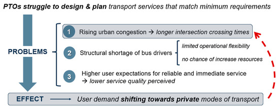
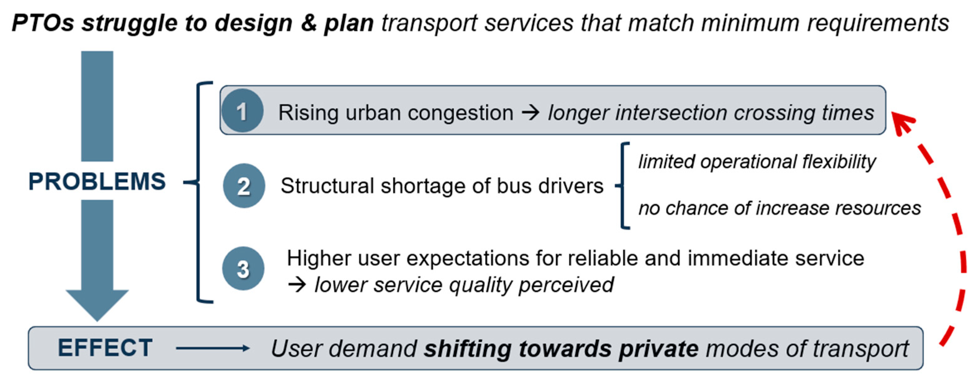
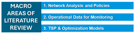
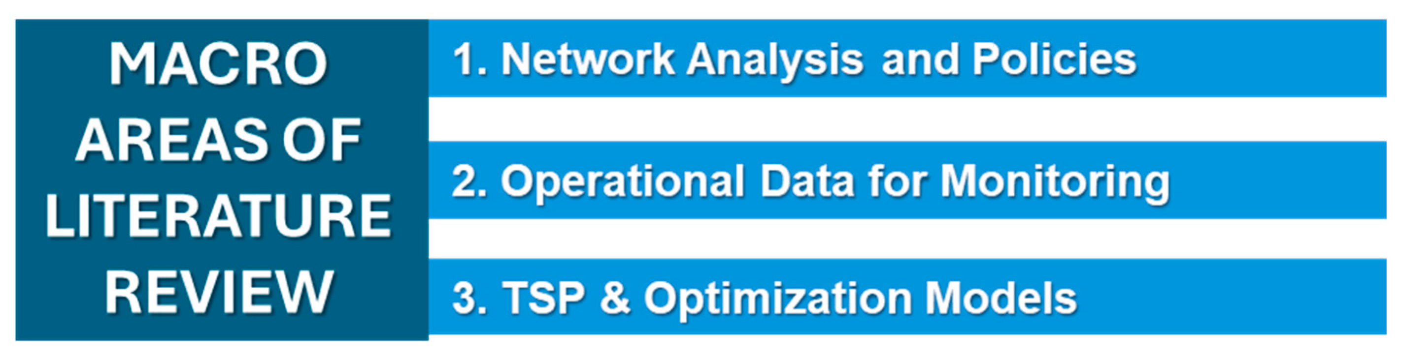
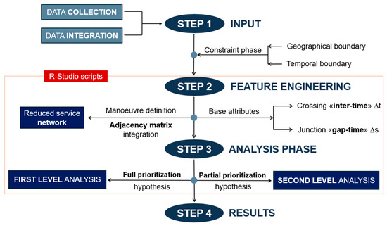
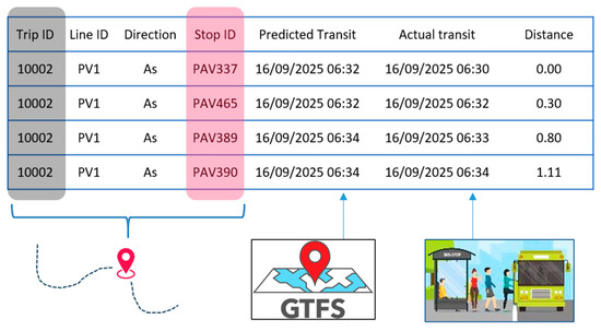


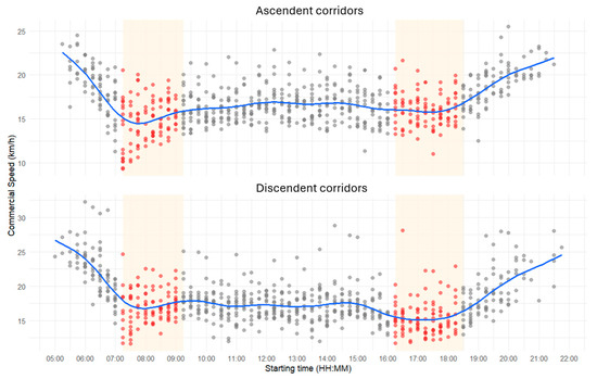
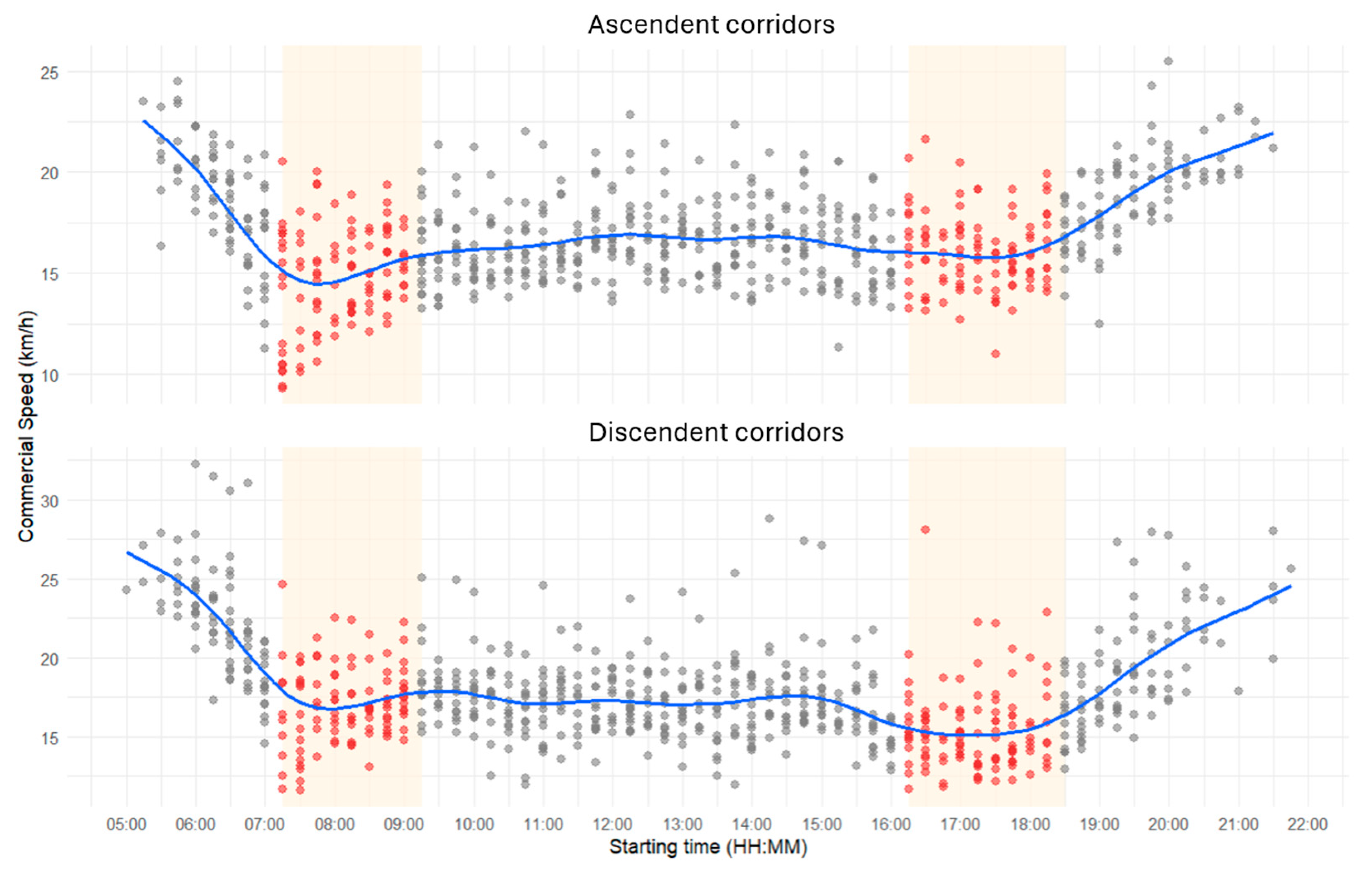
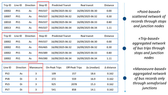
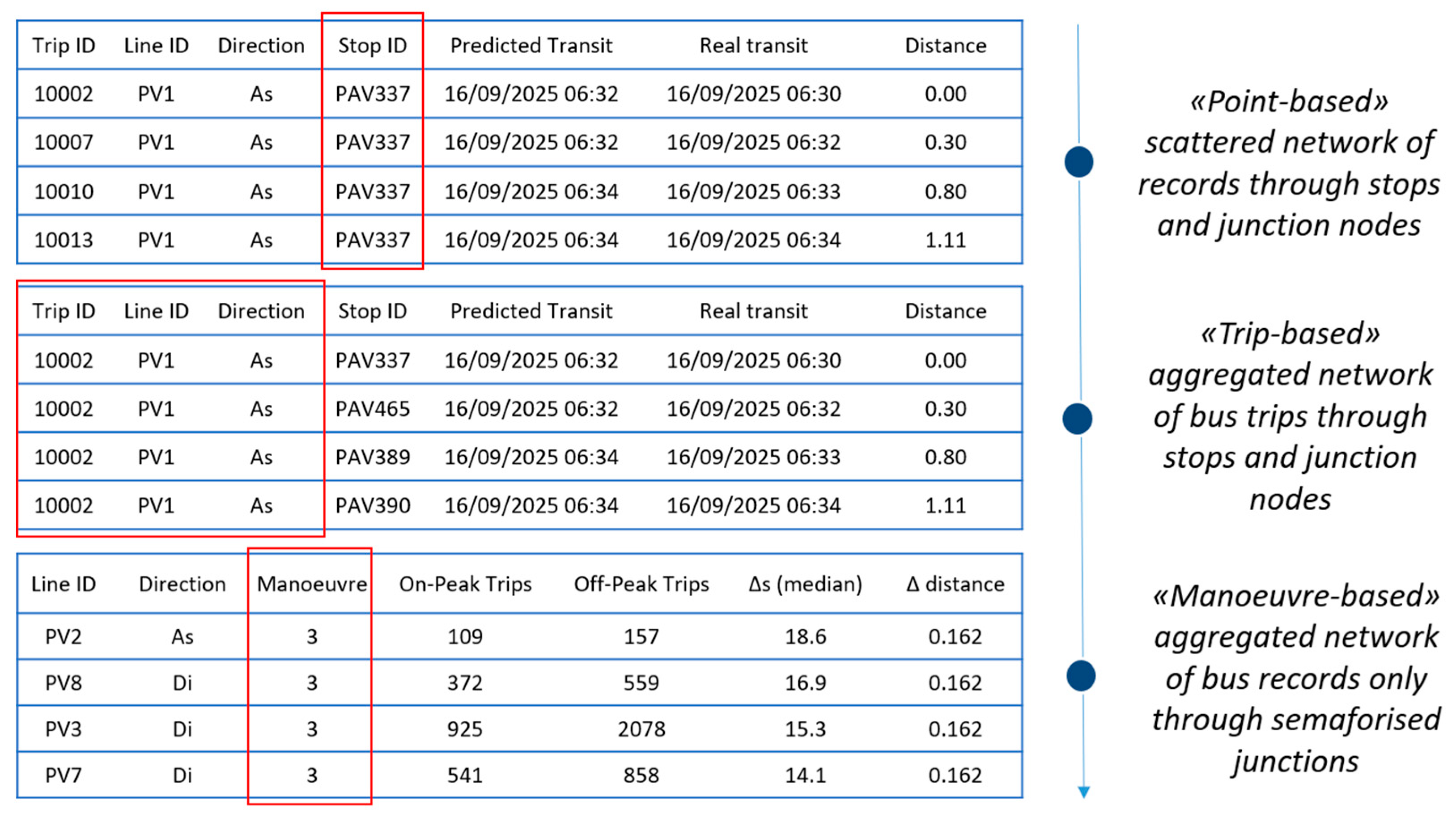
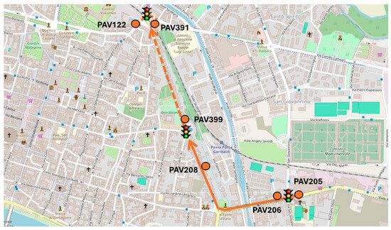
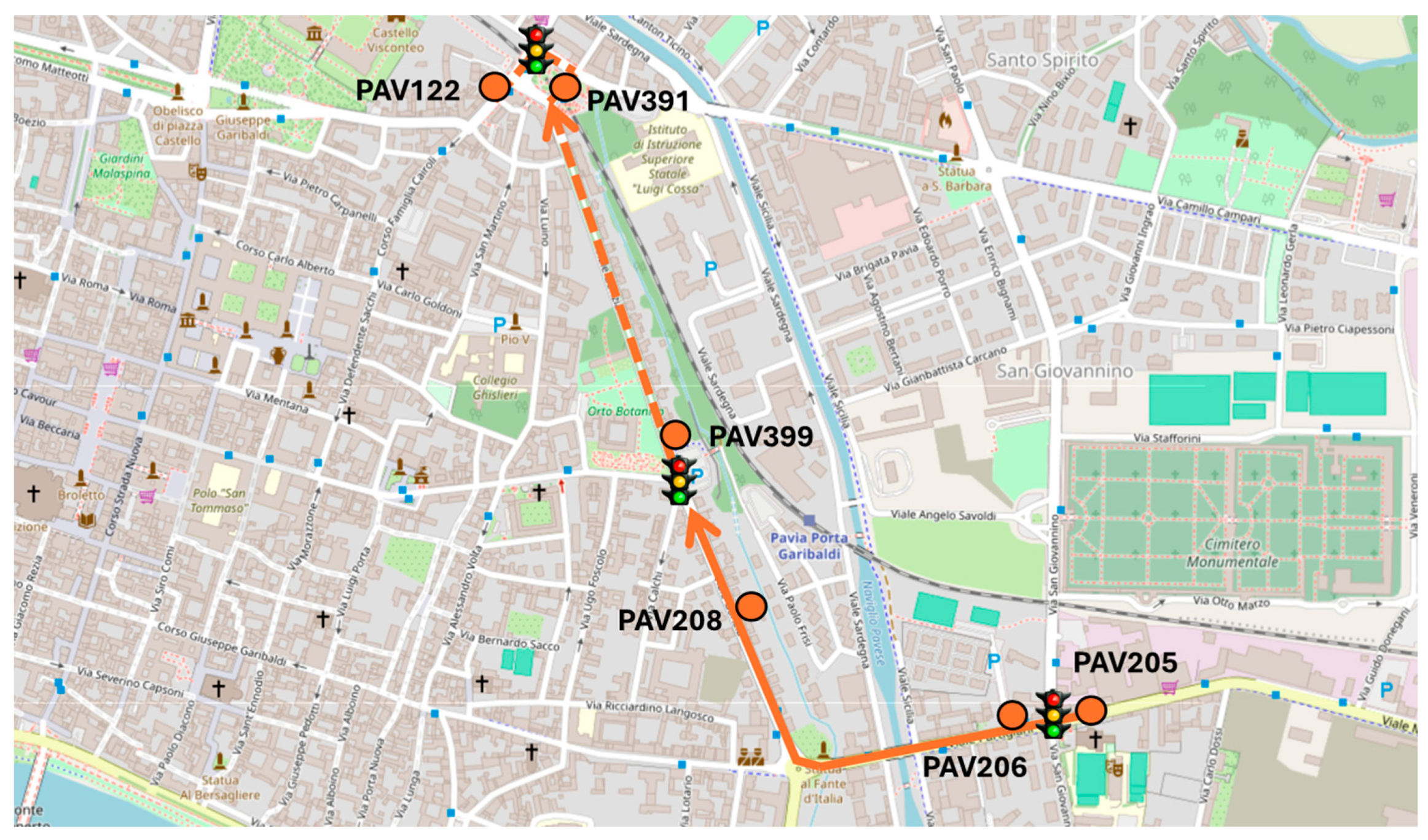
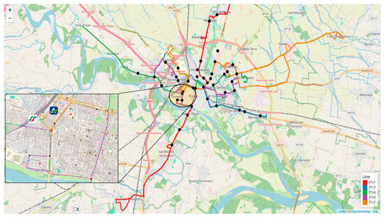
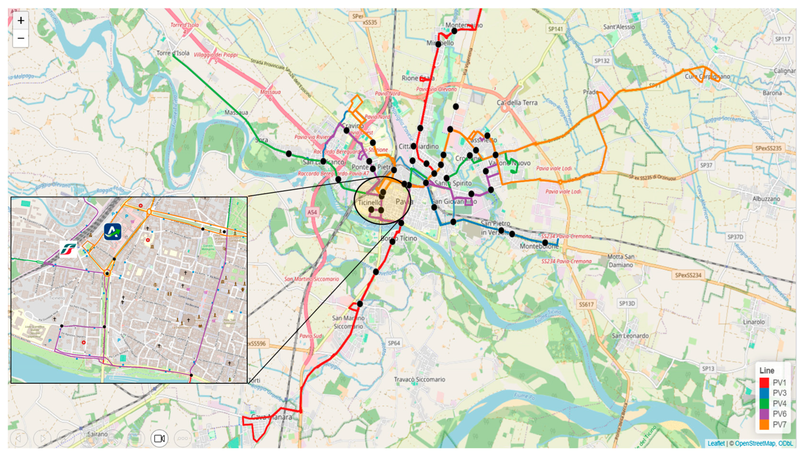
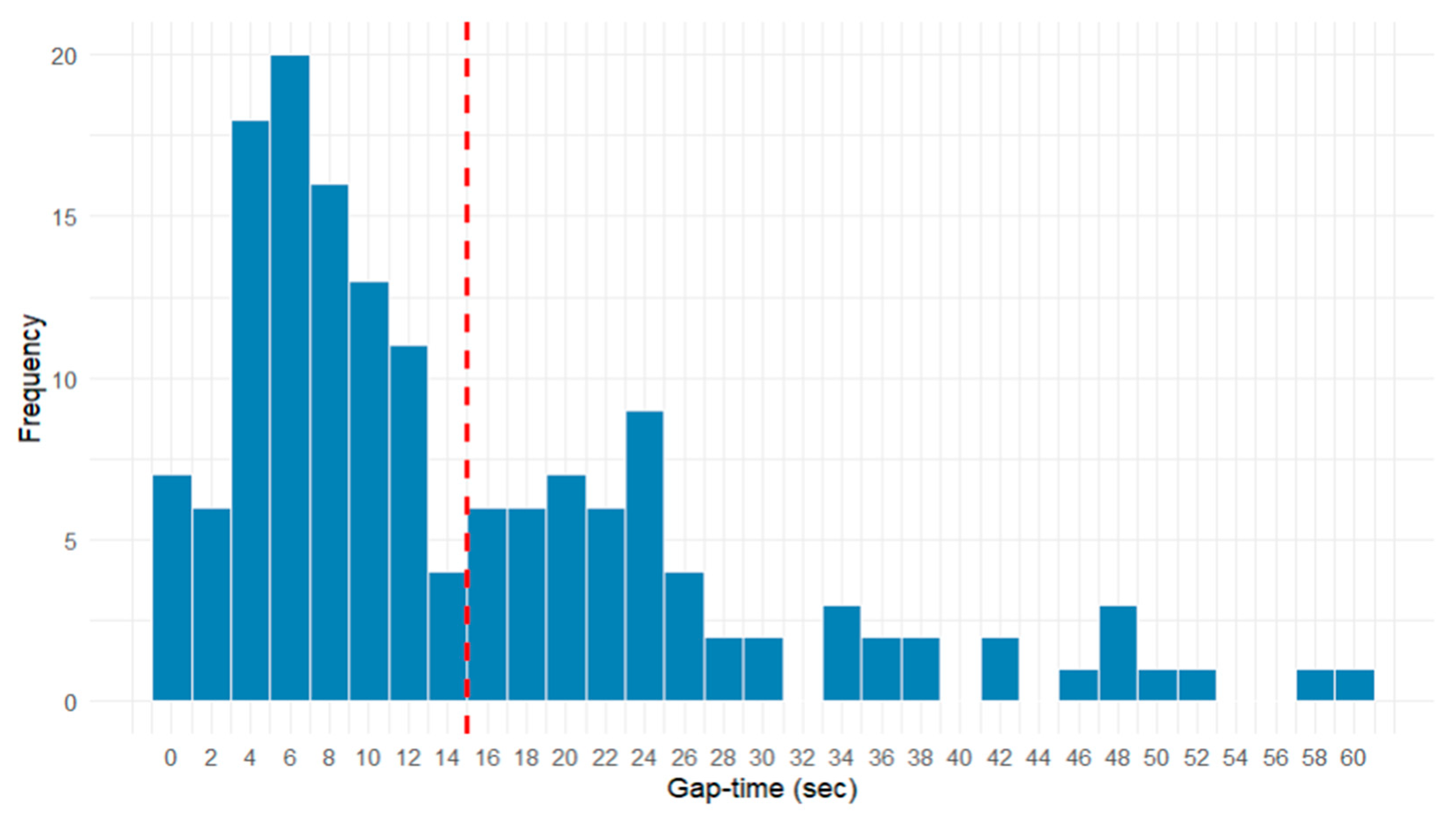
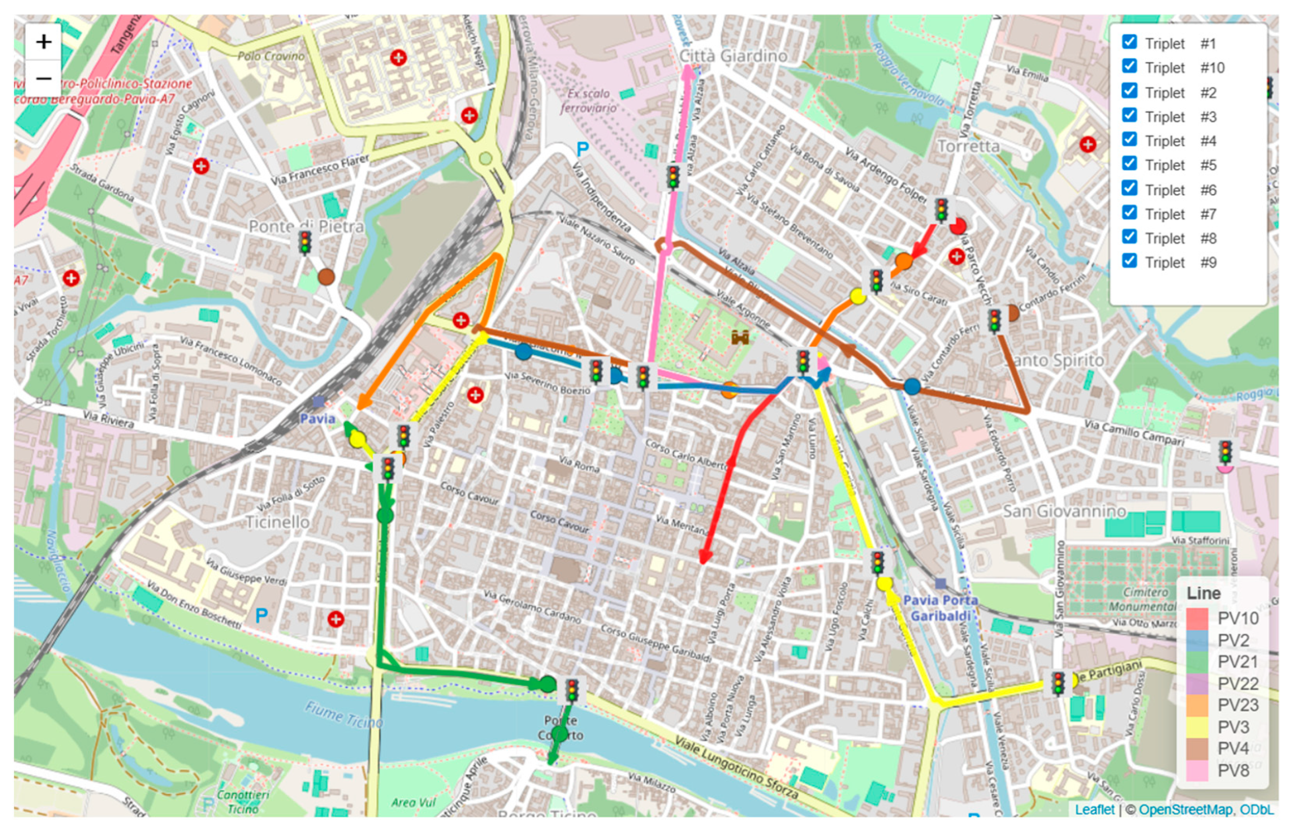
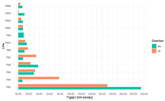
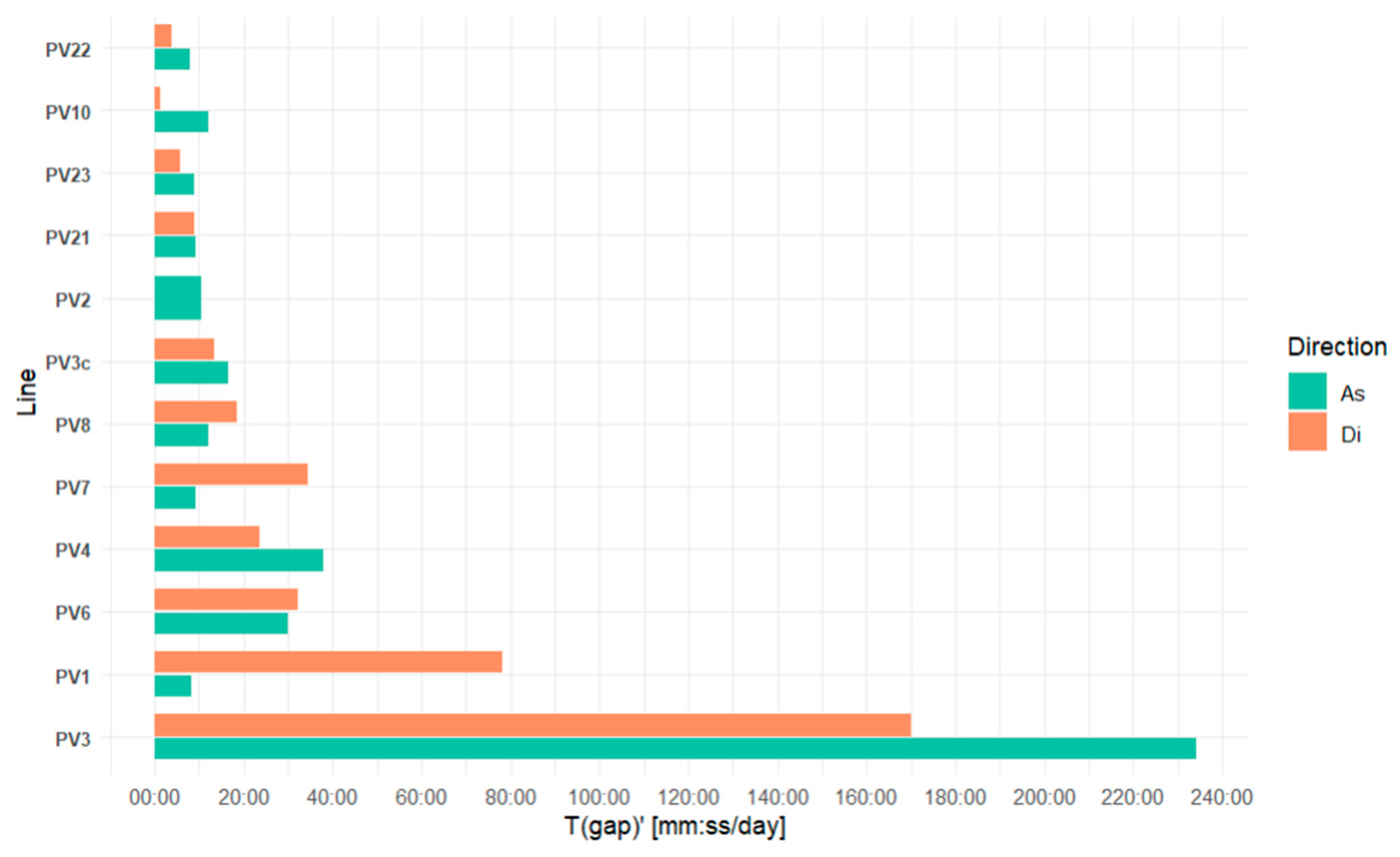
Disclaimer/Publisher’s Note: The statements, opinions and data contained in all publications are solely those of the individual author(s) and contributor(s) and not of MDPI and/or the editor(s). MDPI and/or the editor(s) disclaim responsibility for any injury to people or property resulting from any ideas, methods, instructions or products referred to in the content. |
© 2026 by the authors. Licensee MDPI, Basel, Switzerland. This article is an open access article distributed under the terms and conditions of the Creative Commons Attribution (CC BY) license.