Hydroclimatic Change Detection Based on Observations and Bias-Corrected CMIP6 Projections Under SSP Scenarios

Abstract

This study examines the historical and anticipated effects of climate change on essential hydroclimatic variables (temperature, precipitation, evapotranspiration, and soil moisture) in the Southeastern Anatolia Project (GAP) region of Türkiye, a semi-arid and agriculturally significant basin experiencing heightened water stress. The analysis employs a collection of CMIP6 Global Climate Models (GCM) and integrates three Shared Socioeconomic Pathways (SSP1-2.6, SSP2-4.5, and SSP5-8.5), utilizing statistical bias correction methods such as Delta Change, Quantile Mapping (QM), and Empirical Quantile Mapping (EQM) to improve the regional accuracy of the projections. The ACCESS-CM2 model, validated with data from Türkiye’s Meteorological General Directorate (MGM), was chosen for comprehensive spatial mapping, utilizing Inverse Distance Weighting (IDW) interpolation across seven temporal intervals encompassing past, present, and future periods. The findings indicate a steady increase in temperature and evapotranspiration, especially under high-emission scenarios, with temperature rises above +4 °C and considerable water losses anticipated by century’s end. Soil moisture exhibits a declining tendency, particularly in the southern and eastern regions, signifying increasing drought susceptibility. Precipitation patterns demonstrate significant spatial variability and rising uncertainty, with relative error (RE%) values increasing under SSP5-8.5. Historical data from 1963 to 2022 corroborate these conclusions, indicating a progressive shift towards a warmer and drier regional climate. These observations highlight the importance of climate adaptation strategies and water management in the GAP region. The research provides decision-makers a high-resolution, bias-corrected hydroclimatic dataset.

1. Introduction

In regions with sensitive hydrological systems, where water availability is tightly linked to climatic variability, the impacts of climate change are becoming increasingly pronounced. Altered precipitation regimes, rising temperatures, and shifts in evapotranspiration dynamics are creating complex challenges for water management particularly in semi-arid zones (IPCC, 2021). A compelling example of such vulnerability is Türkiye’s Southeastern Anatolia Project (GAP) region, an ecologically and economically significant basin that has been exposed to growing hydrological stress due to both climatic fluctuations and human-induced pressures [1,2].

Effective adaptation and sustainable water resource planning in these regions require reliable projections of future climate conditions. The Coupled Model Intercomparison Project Phase 6 (CMIP6) offers cutting-edge global climate projections across various Shared Socioeconomic Pathways (SSPs). However, the direct applicability of CMIP6 models to regional hydrological assessments is limited by their coarse spatial resolution and systematic biases in raw outputs [3]. Statistical bias correction methods such as the Delta Change approach, Quantile Mapping (QM), and Empirical Quantile Mapping (EQM) are therefore crucial for improving the agreement between modeled and observed climate variables [4,5].

As climate change continues to reshape environmental and socioeconomic systems, comprehensive scenario-based assessments become essential for informed decision-making [6]. Although uncertainties persist in long-term climate projections [7], the use of climate models particularly when bias-corrected remains indispensable for regional applications [4]. Assessing the impact of climate change on hydroclimatic variables necessitates a combined use of observational datasets and model outputs to establish historical baselines and forecast future conditions under varying emission trajectories [8,9]. Moreover, accounting for the non-stationary nature of climate is critical for robust hydrological modeling [10].

Human-induced climate change has led to significant disruptions in precipitation and evaporation patterns, with increased atmospheric moisture intensifying extreme events [11]. Warming trends are associated with increased flood frequencies in humid regions and worsening droughts in arid zones [12]. CMIP6 models predict regional variations in water availability; increases in precipitation and runoff are expected, particularly at high latitudes [13]. By the century’s end, global annual river discharge is projected to increase by over 13%, intensifying the hydrological cycle and straining freshwater availability in vulnerable regions [14,15].

The integration of Shared Socioeconomic Pathways has improved future climate projections by incorporating varying narratives of global development, adaptation capacity, and mitigation efforts [16,17]. CMIP6 models represent a significant advancement, including new Earth system components and refined climate processes [18]. For example, the BCC-CSM model incorporates updated schemes for turbulent surface fluxes of momentum, energy, and water [19]. Compared to previous generations, CMIP6 models generally exhibit higher climate sensitivity, yielding stronger warming signals and more pronounced hydrological responses [20,21].

In their study, Ref. [22] used CMIP6 climate scenarios and machine learning methods to project future changes in reference evapotranspiration. The results indicate that evapotranspiration is set to increase in the future, particularly as a result of rising temperatures, and that this will have significant implications for agricultural water management. In this study, a new dataset has been developed for global evapotranspiration projections covering the period 1950–2100, using CMIP6 models. The results indicate that evapotranspiration will vary regionally depending on different SSP scenarios and will serve as an important data source for water management studies [23]. Ref. [24] analysed future changes in temperature and precipitation using multiple CMIP6 climate models. The results indicate that significant increases in temperature and changes in precipitation patterns are expected in the future, and that this could affect the hydrological cycle. Ref. [25] analysed changes in temperature, precipitation and evapotranspiration on the Iberian Peninsula using climate models. The results indicate that soil drought will increase, particularly towards the end of the century, due to a decrease in precipitation and an increase in evapotranspiration. In this study, future changes in temperature and precipitation were assessed using CMIP6 climate model projections. The results of the analysis indicate that temperatures will rise and that regional variability in precipitation patterns will increase, depending on the different scenarios. It was emphasised that these changes could have significant impacts, particularly on hydrological processes and water resources [26].

This study provides a spatially explicit, multi-variable assessment of historical and projected hydroclimatic conditions in the GAP region, focusing on four critical variables: precipitation, temperature, soil moisture, and reference evapotranspiration. A multi-model CMIP6 GCM was bias-corrected using Delta Change, QM, and EQM techniques across three emission scenarios (SSP1-2.6, SSP2-4.5, SSP5-8.5). According to performance metrics, the ACCESS-CM2 model was identified as the most consistent with observational records from Türkiye’s Meteorological General Directorate (MGM) and was selected for detailed spatial mapping.

To construct continuous regional estimates, Inverse Distance Weighting (IDW) interpolation was performed across seven temporal slices: historical baseline (1963–1982), far past (1983–2002), recent past (2003–2022), extended baseline (1963–2024), and three future periods-near future (2026–2050), mid-century (2051–2075), and end-century (2076–2100). Reference evapotranspiration was computed using the Penman–Monteith equation [27], with missing daily inputs such as solar radiation and humidity generated via a K-Nearest Neighbor (KNN) weather generator [28].

This research aims to bridge the gap between global climate model outputs and regional-scale water management needs by offering downscaled, bias-corrected, and temporally explicit hydroclimatic projections tailored for one of Türkiye’s most vulnerable and strategically important basins.

This study is driven by the growing need to understand and anticipate the effects of climate change on water resources in semi-arid and hydrologically sensitive regions, where climate variability and anthropogenic pressures intersect. The Southeastern Anatolia Project (GAP) region of Türkiye exemplifies such vulnerability. As one of the country’s most ecologically and agriculturally significant basins, the GAP region encompasses the headwaters of the Euphrates and Tigris Rivers and supports over 20% of Türkiye’s irrigated agriculture [29]. Its strategic role in national food security, energy production, and transboundary water management makes it highly sensitive to climatic shifts. However, rising temperatures, altered precipitation regimes, and increased evapotranspiration are exacerbating hydrological stress in the region, threatening both ecosystem stability and agricultural productivity.

Despite the availability of global climate model projections, their coarse resolution and inherent biases limit their utility for regional planning and hydrological assessments. This study aims to address this gap by producing spatially detailed and bias-corrected projections of four critical hydroclimatic variables: precipitation, temperature, soil moisture, and reference evapotranspiration, using a CMIP6 multi-model. Employing a robust bias correction framework (Delta Change, Quantile Mapping, and Empirical Quantile Mapping) and integrating observed data from Türkiye’s Meteorological General Directorate (MGM), the study enhances the accuracy and regional relevance of climate projections. The inclusion of a K-Nearest Neighbor (KNN) weather generator to simulate missing daily inputs for reference evapotranspiration calculations further strengthens the methodology. By generating high-resolution future climate surfaces across multiple timeframes and emission scenarios, this research offers a valuable dataset for water managers, planners, and policymakers, contributing to informed climate adaptation and sustainable water governance in one of Türkiye’s most climate-vulnerable regions.

2. Materials and Methods

2.1. Data and Study Area

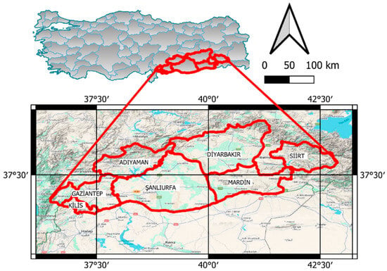
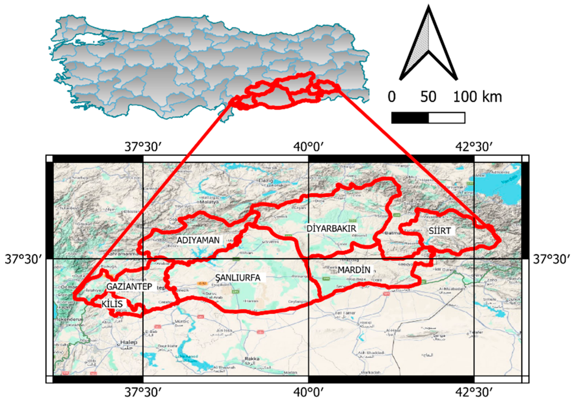
The data used in this study are categorized into two main groups: observed meteorological data and climate model data. Daily climate data used in this study were obtained from meteorological stations located across the nine provinces of the Southeastern Anatolia Project (GAP) region (Figure 1). The dataset was provided by the General Directorate of Meteorology (MGM) under institutional access permissions. The dataset comprises daily observations of relative humidity (RH) (%), wind speed (ws) (m s⁻¹), minimum and maximum air temperature (Tmin and Tmax) (°C), precipitation (pr) (mm), and solar radiation (rsds) (W/m²)).

Figure 1. Location of study area.

2.1.1. Observed Data

Daily climate data from 1963 to 2022 were aggregated for reference evapotranspiration (ET0) computations. Furthermore, incoming shortwave solar radiation (rsds (W/m²)) was obtained from the ERA5 reanalysis dataset.

2.1.2. Climate Model Data

The ACCESS-CM2 global climate model, part of CMIP6, was employed for future forecasts, utilizing eleven GCMs selected for their consistency with observed data. The model’s daily outputs were examined for both the historical period (1950–2014) and the future period (2015–2100). The parameters utilized encompass maximum and minimum air temperature, precipitation, and wind speed. The climate projections were assessed under SSP1-2.6 (low-emission scenario), SSP2-4.5 (medium-emission scenario), and SSP5-8.5 (high-emission scenario).

The Southeastern Anatolia Project (GAP) is built on the land and water resources of the Upper Mesopotamian plains and the Euphrates–Tigris Basin. It spans nine provinces: Adıyaman, Siirt, Diyarbakır, Batman, Kilis, Gaziantep, Mardin, Şırnak, and Şanlıurfa. As a nationwide initiative, GAP seeks to generate income for the local population by harnessing the region’s natural resources, with the broader goal of fostering development through expanded employment opportunities. Despite its potential, the GAP region remains Türkiye’s second least developed area [30,31].

Geographically, the region borders Syria to the south and Iraq to the southeast, covering 57,000 km²-about 7.5% of Türkiye’s total land area and holding 20% of the country’s irrigable land. Its fertile plains are concentrated in the Lower Euphrates and Tigris Basins.

Delta, Quantile mapping and empirical quantile mapping methods were used for bias correction of GCMs. Moreover, KNN-Weather Generator was used to compute future daily relative humidity (RH) and solar radiation (rsds) values based on observed data for 2016–2100 and Penman–Monteith procedure was also used to calculate reference evapotranspiration.

2.2. Bias Correction

The raw GCM data simulations may be insufficient for accurately assessing the impacts on hydrological, agricultural, and other research. This limitation arises from the inadequate and overly coarse geographic resolution of GCM results, typically around 250 km. To mitigate this challenge, scientists employ several methods, with downscaling being a primary approach. Downscaling serves as a bridge between coarse and fine-scale climatic data, enabling more precise analysis and forecasts. Bias correction is an essential component of climate change effect and adaptation research [32,33]. Most climate impact studies have been conducted using Empirical Quantile and Quantile Mapping (QM) [26,34]. To rectify systematic biases in the ACCESS-CM2 model outputs, the Empirical Quantile Mapping (EQM) method was employed for the variables of average temperature, precipitation, wind speed and soil moisture. This procedure guaranteed statistical consistency between model outputs and observed data, hence augmenting the dependability of subsequent projection data.

2.2.1. Delta Method

Delta Approach was used in the literature for downscaling to calculate the difference between the Global Climate Model (GCM) data and the observed data during a given historical time [35]. This delta is then applied to the GCM projections to change and improve the climate data, providing more exact and localized results. The GCM temperature data are downscaled, as described in Equation (1) [36]:

$${\mathrm{T}}_{\mathrm{S}\mathrm{D}}^{\mathrm{D}\mathrm{e}\mathrm{l}\mathrm{t}\mathrm{a}}={\mathrm{T}}_{{\mathrm{G}\mathrm{C}\mathrm{M}}_{\mathrm{S}\mathrm{S}\mathrm{P}}}+({\overline{\mathrm{T}}}_{\mathrm{O}\mathrm{b}\mathrm{s}}-{\overline{\mathrm{T}}}_{\mathrm{G}\mathrm{C}{\mathrm{M}}_{\mathrm{H}\mathrm{i}\mathrm{s}\mathrm{t}}})$$

(1)

where ${\overline{\mathrm{T}}}_{\mathrm{O}\mathrm{b}\mathrm{s}}$ denotes the average observed temperature, and ${\overline{\mathrm{T}}}_{\mathrm{G}\mathrm{C}{\mathrm{M}}_{\mathrm{H}\mathrm{i}\mathrm{s}\mathrm{t}}}$ signifies the mean simulation of historical temperature data from GCM while ${\mathrm{T}}_{\mathrm{S}\mathrm{D}}^{\mathrm{D}\mathrm{e}\mathrm{l}\mathrm{t}\mathrm{a}}$ represent the downscaled data for temperature. Subscript Obs signifies the observational values, while ${\mathrm{G}\mathrm{C}\mathrm{M}}_{\mathrm{S}\mathrm{S}\mathrm{P}}$ denotes the GCM’s SSP outputs for the future period.

2.2.2. Quantile Mapping (QM)

There have been numerous applications of QM, a statistical downscaling technique, in different fields of study [2,37]. Quantum mechanics equations determine the modeled probability distribution in respect to the observed probability distribution. Equation (2) is utilized for evaluation, while Equation (3) is used for subsequent downscaling.

$${\mathrm{P}}_{\mathrm{t}}^{\mathrm{E}\mathrm{v}\mathrm{a}\mathrm{l}}={\mathrm{I}\mathrm{n}\mathrm{v}\mathrm{C}\mathrm{D}\mathrm{F}}_{{\mathrm{P}}_{\mathrm{t}}}^{\mathrm{O}\mathrm{b}\mathrm{s}}\left({\mathrm{C}\mathrm{D}\mathrm{F}}_{{\mathrm{P}}_{\mathrm{t}}}^{\mathrm{H}\mathrm{i}\mathrm{s}\mathrm{t}}\left({\mathrm{P}}_{\mathrm{t},\mathrm{H}\mathrm{i}\mathrm{s}\mathrm{t}}\right)\right)$$

(2)

$${\mathrm{P}}_{\mathrm{t}}^{\mathrm{P}\mathrm{r}\mathrm{e}\mathrm{d}}={\mathrm{I}\mathrm{n}\mathrm{v}\mathrm{C}\mathrm{D}\mathrm{F}}_{{\mathrm{P}}_{\mathrm{t}}}^{\mathrm{O}\mathrm{b}\mathrm{s}}\left({\mathrm{C}\mathrm{D}\mathrm{F}}_{{\mathrm{P}}_{\mathrm{t}}}^{\mathrm{H}\mathrm{i}\mathrm{s}\mathrm{t}}\left({\mathrm{P}}_{\mathrm{t},\mathrm{S}\mathrm{S}\mathrm{P}}\right)\right)$$

(3)

where ${\mathrm{C}\mathrm{D}\mathrm{F}}_{{\mathrm{P}}_{\mathrm{t}}}^{\mathrm{H}\mathrm{i}\mathrm{s}\mathrm{t}}$ presents the cumulative distribution function (CDF) based on historical period; ${\mathrm{I}\mathrm{n}\mathrm{v}\mathrm{C}\mathrm{D}\mathrm{F}}_{{\mathrm{P}}_{\mathrm{t}}}^{\mathrm{O}\mathrm{b}\mathrm{s}}$ represents the inverse cumulative distribution function (CDF) based on observational data. ${\mathrm{P}}_{\mathrm{t},\mathrm{H}\mathrm{i}\mathrm{s}\mathrm{t}}$ represent each precipitation time series in the historical period of GCMs, and ${\mathrm{P}}_{\mathrm{t},\mathrm{S}\mathrm{S}\mathrm{P}}$ represent each precipitation time series in SSPs scenarios.

2.2.3. Empirical Quantile Mapping (EQM)

The Empirical Quantile Mapping method is a variation on the usual QM approach. Similar to Quantile Mapping, it involves aligning the cumulative distribution functions of GCMs with empirical data. Nonetheless, EQM makes further alterations to the data to improve its durability and accuracy, particularly during extreme weather events.

$${\mathrm{P}}_{\mathrm{t}}^{\mathrm{E}\mathrm{v}\mathrm{a}\mathrm{l}}={\mathrm{I}\mathrm{n}\mathrm{v}\mathrm{E}\mathrm{C}\mathrm{D}\mathrm{F}}_{{\mathrm{P}}_{\mathrm{t}-\mathrm{C}\mathrm{a}\mathrm{l}}}^{\mathrm{S}\mathrm{t}\mathrm{a}\mathrm{t}}\left({\mathrm{E}\mathrm{C}\mathrm{D}\mathrm{F}}_{{\mathrm{P}}_{\mathrm{t}-\mathrm{C}\mathrm{a}\mathrm{l}}}^{\mathrm{H}\mathrm{i}\mathrm{s}\mathrm{t}}\left({\mathrm{P}}_{\mathrm{t}-\mathrm{E}\mathrm{v}\mathrm{a}\mathrm{l}}^{\mathrm{G}\mathrm{C}\mathrm{M}}\right)\right)$$

(4)

$${\mathrm{P}}_{\mathrm{t}}^{\mathrm{P}\mathrm{r}\mathrm{e}\mathrm{d}}={\mathrm{I}\mathrm{n}\mathrm{v}\mathrm{E}\mathrm{C}\mathrm{D}\mathrm{F}}_{{\mathrm{P}}_{\mathrm{t}-\mathrm{H}\mathrm{i}\mathrm{s}\mathrm{t}}}^{\mathrm{S}\mathrm{t}\mathrm{a}\mathrm{t}}\left({\mathrm{E}\mathrm{C}\mathrm{D}\mathrm{F}}_{{\mathrm{P}}_{\mathrm{t}-\mathrm{H}\mathrm{i}\mathrm{s}\mathrm{t}}}^{\mathrm{H}\mathrm{i}\mathrm{s}\mathrm{t}}\left({\mathrm{P}}_{\mathrm{t}-\mathrm{S}\mathrm{S}\mathrm{P}}^{\mathrm{G}\mathrm{C}\mathrm{M}}\right)\right)$$

(5)

A thorough study of statistical downscaling techniques, particularly EQM, was presented by Ref. [38]. The EQM employs the empirical cumulative distribution function (ECDF) as specified in Equation (4). Equation (5) is utilized for subsequent downscaling, but Equation (4) is employed for evaluation.

2.3. KNN-Weather Generator

The KNN-Weather Generator employs a conditional resampling technique, deriving values from existing datasets while adhering to specified conditional relationships [39]. This procedure is notably simple, making it an appealing choice. The K closest neighbor (KNN) resampling technique is acknowledged as a highly efficient non-parametric approach for producing meteorological data. The KNN method relies on identifying analogous patterns in historical weather data that closely correspond to the conditions of the target year. The model requires input files that include data from the target year as well as historical data. The climatic conditions determined by using this methodology mirror prior observations in the designated year. The KNN method circumvents the necessity for predetermined mathematical functions to forecast target variables [39].

This strategy primarily entails selecting a specific number of days that possess similar characteristics to the day in question. A day is randomly chosen for resampling, representing the subsequent day within the simulation timeframe. This nearest-neighbor methodology involves the concurrent sampling of multiple meteorological variables, including precipitation and temperature. The resampling method employs observed data, allowing for replacement when required. Further insights can be found in a study conducted by Ref. [39].

2.4. Reference Evapotranspiration (ET₀) Calculations

Daily reference evapotranspiration values were computed using the aggregated observed and bias-corrected model datasets, adhering to the FAO Penman–Monteith methodology. The Penman–Monteith method has been widely utilized due to its incorporation of multiple climatic variables, such as wind speed and relative humidity [40,41]. The monthly ET₀ was computed as follows:

$${\mathrm{E}\mathrm{T}}_0={\displaystyle \frac{0.408∆\left({\mathrm{R}}_{\mathrm{n}}-\mathrm{G}\right)+\mathrm{\gamma }\frac{900}{\mathrm{T}+273}\mathrm{w}\mathrm{s}({\mathrm{e}}_{\mathrm{s}}-{\mathrm{e}}_{\mathrm{a}})}{∆+\mathrm{\gamma }(1+0.34\mathrm{w}\mathrm{s})}}$$

(6)

where e_s is the saturation vapor pressure (kPa), ws is the mean wind speed (m/s), e_a is the actual vapor pressure (kPa), G is the ground heat flux (MJ/m²day), R_n is the ground net radiation (MJ/m²day), T = (Tmax + Tmin)/2, and γ is the psychrometric constant (kPa/°C). Utilizing the ET₀ data, the SPEI-12 and PDSI indices were computed.

2.5. Performance Assessment of GCMs

Four statistical criteria were employed to evaluate the fidelity of CMIP6 simulations in representing climatic variables when compared to MGM and ERA5 reanalysis data. Nash Sutcliffe Efficiency (NSE), Root Mean Square Error (RMSE), Mean Absolute Error (MAE), Correlation Coefficient (R) and Index of Agreement (IO) are among these metrics. The application of these statistical criteria provides a comprehensive assessment of the CMIP6 models’ ability to represent climate parameters. The following metrics were calculated to identify the optimal model by comparing the MGM and CMIP6 values:

$$\mathrm{M}\mathrm{A}\mathrm{E}={\displaystyle \frac{1}{\mathrm{N}}}\sum _{\mathrm{i}=1}^{\mathrm{n}} \left|\left({\mathrm{C}\mathrm{M}\mathrm{I}\mathrm{P}6}_{\mathrm{i}}-{\mathrm{M}\mathrm{G}\mathrm{M}}_{\mathrm{i}}\right)\right|$$

(7)

$$\mathrm{R}\mathrm{M}\mathrm{S}\mathrm{E}=\sqrt{{\displaystyle \frac{1}{\mathrm{N}}}\sum _{\mathrm{i}=1}^{\mathrm{N}}{\left({\mathrm{M}\mathrm{G}\mathrm{M}}_{\mathrm{i}}-{\mathrm{C}\mathrm{M}\mathrm{I}\mathrm{P}6}_{\mathrm{i}}\right)}^2}$$

(8)

$$\mathrm{N}\mathrm{S}\mathrm{E}=1-\left[{\displaystyle \frac{{\sum }_{\mathrm{i}=1}^{\mathrm{n}}{\left({\mathrm{C}\mathrm{M}\mathrm{I}\mathrm{P}6}_{\mathrm{i}}-{\mathrm{M}\mathrm{G}\mathrm{M}}_{\mathrm{i}}\right)}^2}{{\sum }_{\mathrm{i}=1}^{\mathrm{n}}{\left(\mathrm{M}\mathrm{G}{\mathrm{M}}_{\mathrm{i}}-\overline{{\mathrm{M}\mathrm{G}\mathrm{M}}_{\mathrm{i}}}\right)}^2}}\right]$$

(9)

$$\mathrm{I}\mathrm{n}\mathrm{d}\mathrm{e}\mathrm{x} \mathrm{o}\mathrm{f} \mathrm{A}\mathrm{g}\mathrm{r}\mathrm{e}\mathrm{e}\mathrm{m}\mathrm{e}\mathrm{n}\mathrm{t}=1-\left[{\displaystyle \frac{{\sum }_{\mathrm{i}=1}^{\mathrm{n}}{\left({{\mathrm{M}\mathrm{G}\mathrm{M}}_{\mathrm{i}}-\mathrm{C}\mathrm{M}\mathrm{I}\mathrm{P}6}_{\mathrm{i}}\right)}^2}{{\sum }_{\mathrm{i}=1}^{\mathrm{n}}{\left(\left(\left|\mathrm{C}\mathrm{M}\mathrm{I}\mathrm{P}{6}_{\mathrm{i}}-\overline{{\mathrm{M}\mathrm{G}\mathrm{M}}_{\mathrm{i}}}\right|\right)+\left({\mathrm{M}\mathrm{G}\mathrm{M}}_{\mathrm{i}}-\overline{{\mathrm{M}\mathrm{G}\mathrm{M}}_{\mathrm{i}}}\right)\right)}^2}}\right]$$

(10)

$$\mathrm{R}={\displaystyle \frac{{\sum }_{\mathrm{i}=1}^{\mathrm{n}} \left({\mathrm{C}\mathrm{M}\mathrm{I}\mathrm{P}6}_{\mathrm{i}}-{\mathrm{C}\mathrm{M}\mathrm{I}\mathrm{P}6}_{\mathrm{m}\mathrm{e}\mathrm{a}\mathrm{n}}\right)\times \left({\mathrm{M}\mathrm{G}\mathrm{M}}_{\mathrm{i}}-{\mathrm{M}\mathrm{G}\mathrm{M}}_{\mathrm{m}\mathrm{e}\mathrm{a}\mathrm{n}}\right)}{\sqrt{{\sum }_{\mathrm{i}=1}^{\mathrm{n}} {\left({\mathrm{C}\mathrm{M}\mathrm{I}\mathrm{P}6}_{\mathrm{i}}-{\mathrm{C}\mathrm{M}\mathrm{I}\mathrm{P}6}_{\mathrm{m}\mathrm{e}\mathrm{a}\mathrm{n}}\right)}^2\times {\sum }_{\mathrm{i}=1}^{\mathrm{n}} {\left({\mathrm{M}\mathrm{G}\mathrm{M}}_{\mathrm{i}}-{\mathrm{M}\mathrm{G}\mathrm{M}}_{\mathrm{m}\mathrm{e}\mathrm{a}\mathrm{n}}\right)}^2}}}$$

(11)

$$\mathrm{R}\mathrm{E}={\displaystyle \frac{\left({\mathrm{C}\mathrm{M}\mathrm{I}\mathrm{P}6}_{\mathrm{i}}-{\mathrm{M}\mathrm{G}\mathrm{M}}_{\mathrm{i}}\right)}{{\mathrm{M}\mathrm{G}\mathrm{M}}_{\mathrm{i}}}}\times 100$$

(12)

Relative Error was used to determine the changes in the variables. Here, $\mathrm{C}\mathrm{M}\mathrm{I}\mathrm{P}{6}_{\mathrm{i}}$ is the value of the CMIP 6 model and $\mathrm{M}\mathrm{G}\mathrm{M}$ is the measured value. The efficacy of CMIP 6 models is deemed satisfactory when the MAE and RMSE values approach 0 and the R values approach.

2.6. Inverse Distance Weighting (IDW)

It operates under the premise that proximity correlates with similarity more than distance does [42]. The IDW algorithm can utilize the observed values in the vicinity of the forecast location to estimate the value for any unmeasured site. The measured values nearest to the forecast site are likely to exert greater influence on the anticipated value than those situated farther away. The IDW assumes that all measured points exhibit a diminishing location effect with increasing distance. Proximal points are of greater significance than those that are more distant; thus, the term “inverse distance weighting” is proposed.

3. Results

Climate parameters of the GAP region were evaluated separately for both past and future. The past period was divided into baseline (1963–1982), near past (2003–2022) and far past (1983–2002). The future periods are divided into baseline (1963–2022), near future (2026–2050), mid future (2051–2075) and far future (2076–2100). Considering these periods, average temperature, reference evapotranspiration, soil moisture and precipitation were evaluated separately.

3.1. Assessment of the GCMs and Bias Correction Methods

Based on all stations, EQM demonstrated the best overall performance (Table 1). It consistently achieved lower RMSE and MAE values, along with higher IOA and NSE scores compared to Delta and QM. While differences in correlation (R) were minimal across methods, EQM generally outperformed the others in terms of accuracy and agreement, making it the most reliable bias correction method overall. For example, the best overall performance was achieved by the EQM method in Siirt. It recorded the lowest RMSE (4.574) and MAE (2.96), along with the highest R (0.919), IOA (0.959), and NSE (0.839) values among all stations and methods. This indicates that EQM provided the most accurate and reliable bias correction results for Siirt.

Table 1. Performance assessment of bias correction methods.

Method	RMSE	R	MAE	IOA	NSE
Adıyaman
Delta	5.009	0.893	3.75	0.936	0.793
QM	5.023	0.893	3.55	0.945	0.792
EQM	5.101	0.893	3.32	0.945	0.785
Batman
Delta	4.845	0.9	3.49	0.946	0.81
QM	4.988	0.899	3.44	0.948	0.798
EQM	4.961	0.9	3.33	0.949	0.801
Cizre
Delta	6.6	0.893	5.51	0.915	0.515
QM	4.358	0.895	2.86	0.946	0.788
EQM	4.317	0.896	2.67	0.947	0.792
Diyarbakır
Delta	4.899	0.893	3.46	0.944	0.796
QM	5.032	0.893	3.46	0.945	0.785
EQM	4.978	0.895	3.37	0.945	0.789
Gaziantep
Delta	5.519	0.865	4.22	0.92	0.746
QM	5.832	0.863	3.91	0.929	0.717
EQM	5.521	0.873	3.63	0.934	0.746
Kilis
Delta	5.459	0.868	3.99	0.93	0.713
QM	5.18	0.867	3.65	0.931	0.741
EQM	5.285	0.865	3.4	0.93	0.73
Mardin
Delta	4.872	0.867	3.28	0.931	0.735
QM	4.877	0.867	3.28	0.931	0.734
EQM	4.879	0.867	3.23	0.931	0.734
Şanlıurfa
Delta	9.071	0.869	8.19	0.801	0.589
QM	7.872	0.856	5.12	0.924	0.69
EQM	7.276	0.868	4.55	0.931	0.735
Siirt
Delta	4.832	0.911	3.79	0.944	0.82
QM	4.968	0.908	3.65	0.952	0.81
EQM	4.574	0.919	2.96	0.959	0.839

The ACCESS-CM2 model was selected due to its strong overall performance, showing a good balance between accuracy and reliability. It achieved a low RMSE (5.101) and MAE (3.32), a high correlation coefficient (R = 0.893), and strong agreement metrics (IOA = 0.945, NSE = 0.785), making it one of the most consistent and well-performing models under SSP5-8.5 for Adıyaman (Table 2).

Table 2. Evaluation of GCMs of soil moisture under SSP5-8.5 for Adıyaman.

Method	RMSE	R	MAE	IOA	NSE
ACCESS-CM2
EQM	5.101	0.893	3.32	0.945	0.785
CESM2
EQM	5.477	0.876	3.63	0.936	0.752
CMCC-ESM2
EQM	5.08	0.894	3.36	0.945	0.787
MIROC6
EQM	5.177	0.889	3.34	0.943	0.779
MRI-ESM2-0
EQM	5.847	0.859	3.81	0.927	0.718
NorESM2-LM
EQM	4.683	0.909	3.07	0.953	0.819

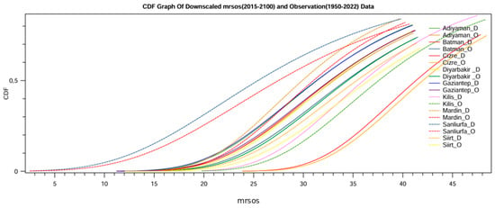
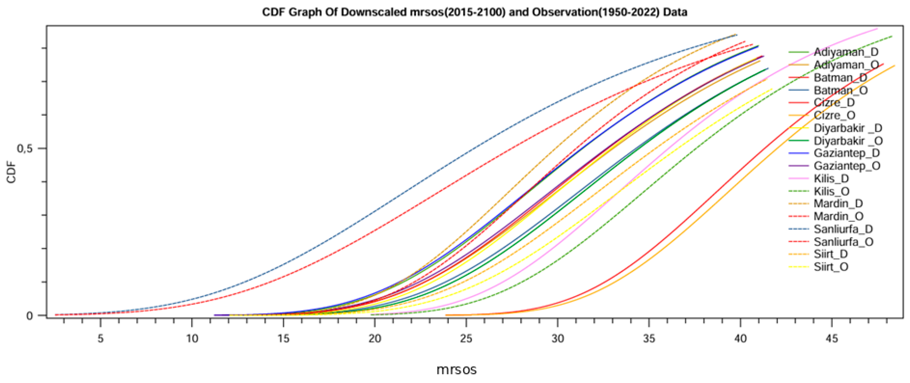
Figure 2 shows the Cumulative Distribution Function (CDF) of downscaled surface soil moisture (mrsos) for the period 2015–2100 under the SSP1-2.6 scenario, compared with observed data from 1950–2022. The downscaled model outputs are labeled with “_D” and the observations with “_O” for each station. Overall, the downscaled data closely follow the observed distributions across most stations, indicating that the bias correction and downscaling approach effectively preserved the statistical properties of soil moisture. While minor deviations are visible in certain locations, such as Cizre and Şanlıurfa, the general alignment suggests a strong agreement between modeled and observed data. This consistency supports the reliability of the downscaled projections under SSP1-2.6.

Figure 2. Cumulative Distribution Frequency (CDF) graph of downscaled soil moisture under SSP1–2.6.

3.2. Evaluation of the Past Climate Variables (1963–2022)

3.2.1. Precipitation (PR)

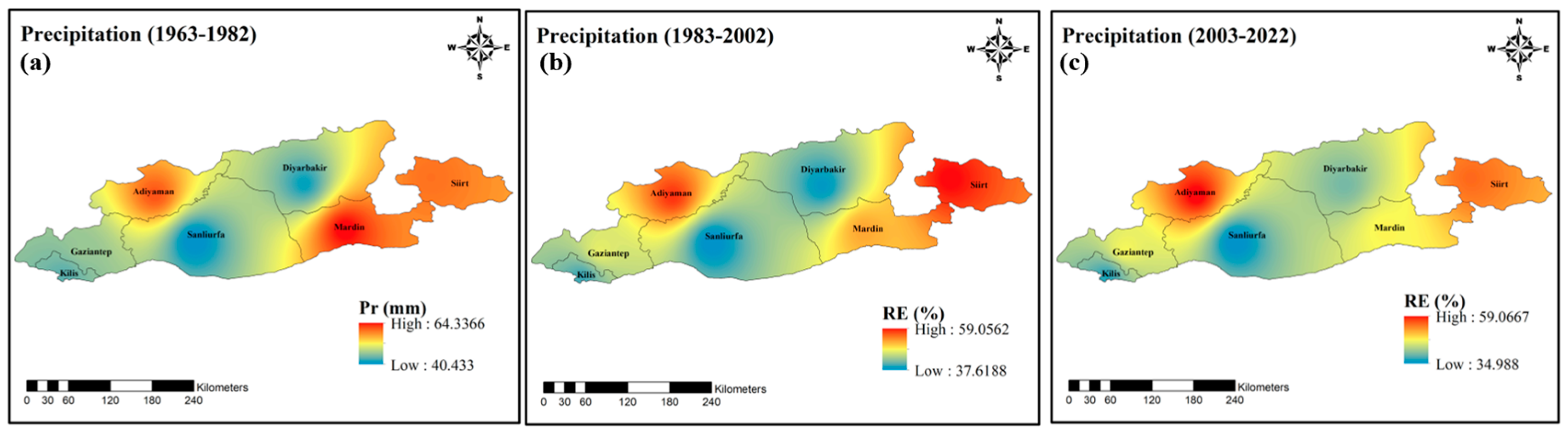
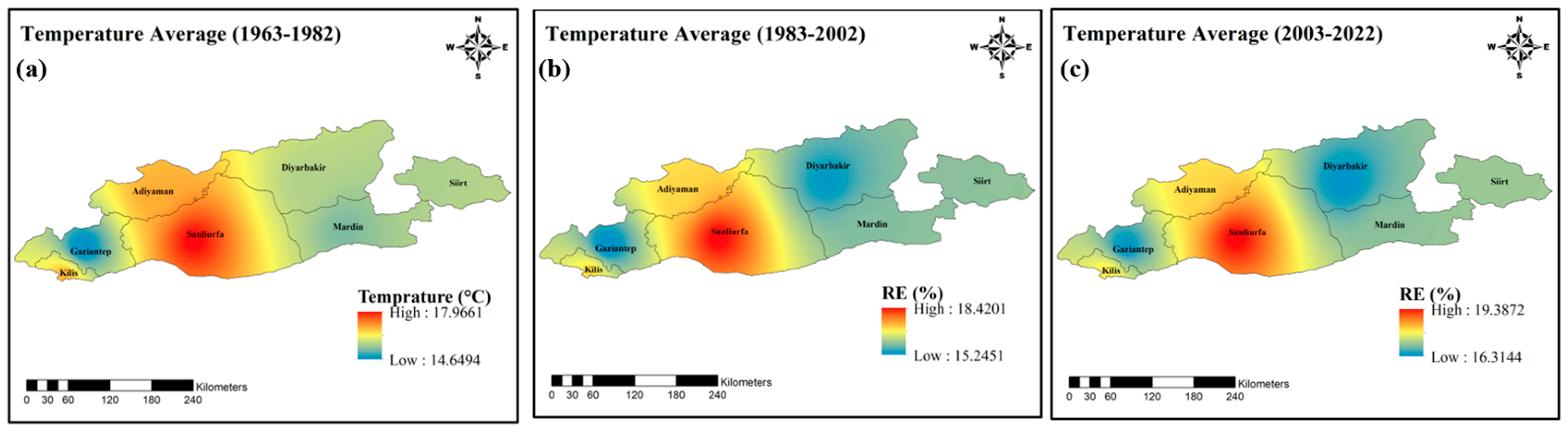
This visualization reveals how four key hydrometeorological variables (precipitation, average temperature, evapotranspiration and soil moisture) have changed over three time periods (1963–1982/1983–2002/2003–2022) covering the last six decades of the GAP region. Changes in each parameter dramatically reflect the climatic transformation of the region.

Precipitation (PR) maps show a decreasing trend that has become more pronounced over time, especially in the southeast. While there was a more widespread and balanced distribution in the 1963–1982 period, both the amount and the area of precipitation are shrinking in the recent period. This shows that the drought pressure in the region is gradually increasing (Figure 3).

Figure 3. Spatial variation in observed precipitation: (a) Baseline (1963–1982), (b) Relative error (%) of PR for far past (1983–2002), (c) relative error (%) of PR for near past (2003–2022).

3.2.2. Average Temperature (Tave)

Temperature (Tave) changes are quite clear: Temperatures have been rising steadily with each period. This increase has intensified, especially in the last 20 years. Increasing temperature stands out as one of the main factors that trigger all other variables (Figure 4).

Figure 4. Spatial variation in observed average temperature: (a) Baseline (1963–1982), (b) Relative error (%) of Tave for far past (1983–2002), (c) relative error (%) of Tave for near past (2003–2022).

3.2.3. Reference Evapotranspiration (ET0)

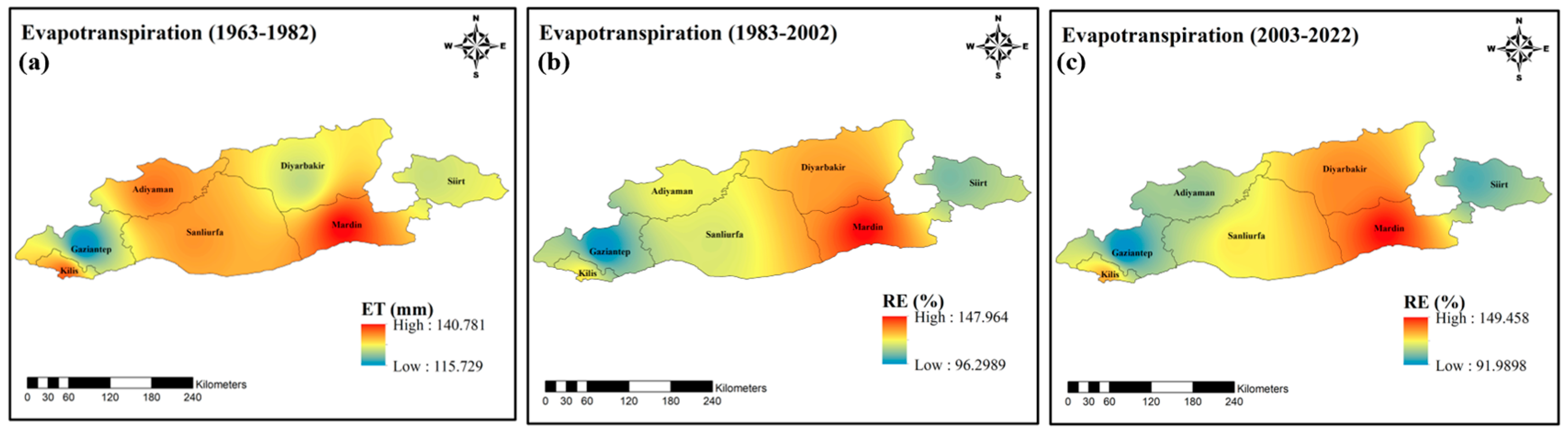
Evapotranspiration (ET) maps show that evaporation–transpiration rates have increased significantly with the increase in temperature. This increase poses a serious threat to surface water and soil moisture. It is noteworthy that ET values have recently spread over large areas of the GAP (Figure 5).

Figure 5. Spatial variation in observed reference evapotranspiration: (a) Baseline (1963–1982), (b) Relative error (%) of ET for far past (1983–2002), (c) relative error (%) of ET for near past (2003–2022).

3.2.4. Soil Moisture (SM)

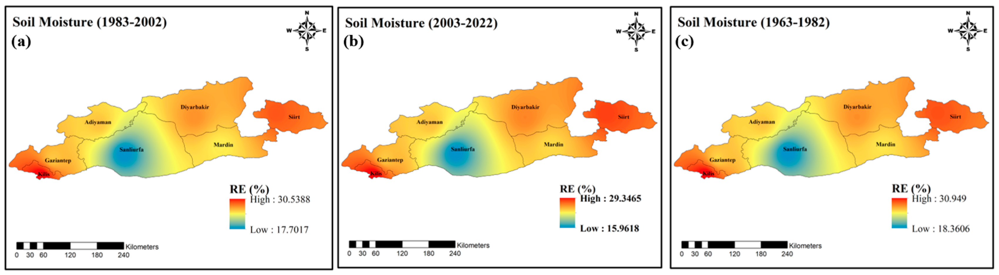
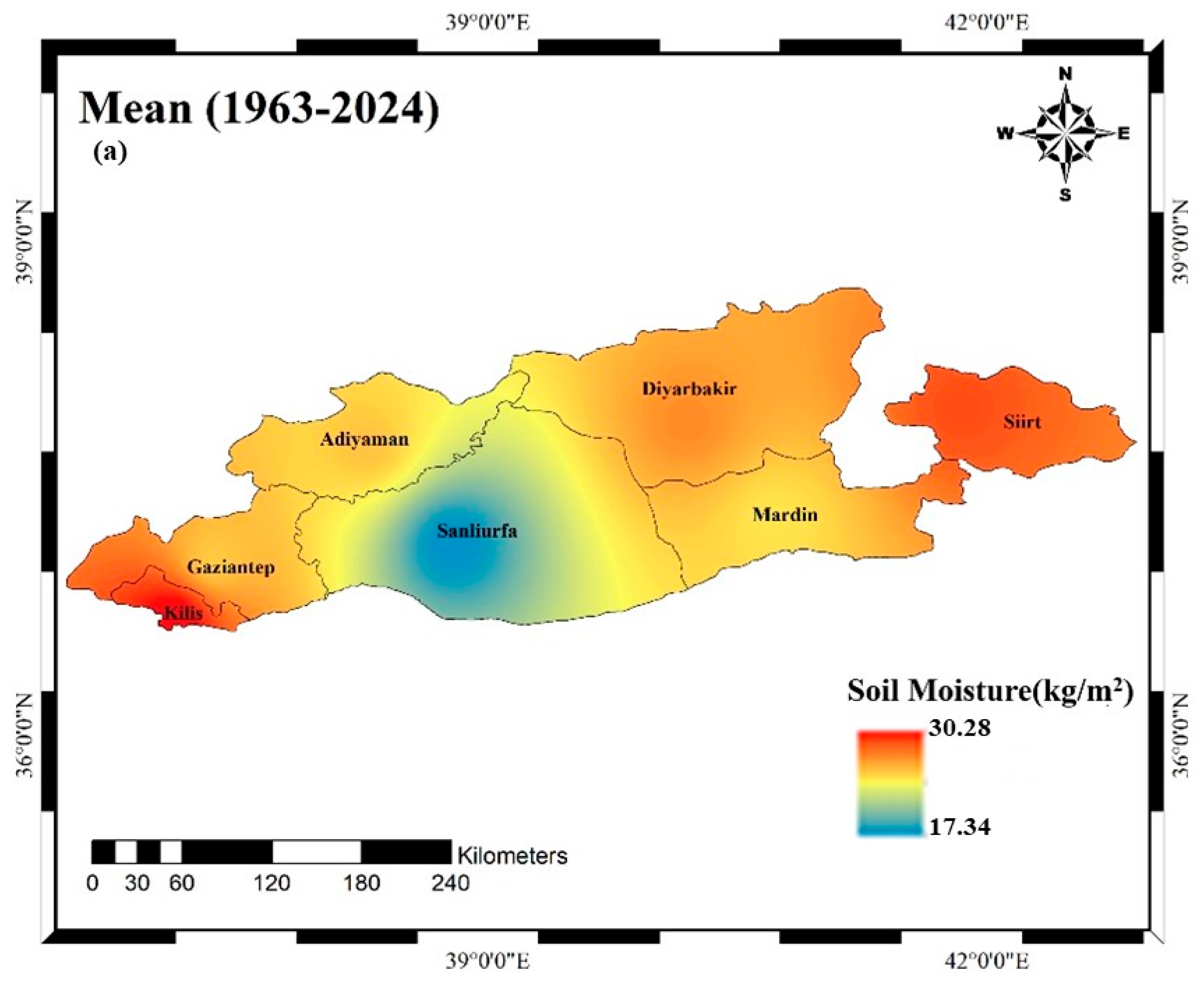
Soil Moisture data complement this picture. Especially in the “near past” period, moisture levels have decreased dramatically. This is a critical signal that directly affects both vegetation and agricultural production.

When these four variables are evaluated together, it is clear that the region has undergone a strong climatic transformation in the last few decades in the direction of both warming, aridification and disruption of the hydrological balance. Careful monitoring of these trends is of great importance to guide future projections (Figure 6).

Figure 6. Spatial variation in observed soil moisture: (a) Baseline (1963–1982), (b) Relative error (%) of SM for far past (1983–2002), (c) relative error (%) of SM for near past (2003–2022).

3.3. Evaluation of Projected Climate Variables (2026–2100)

3.3.1. Precipitation (PR)

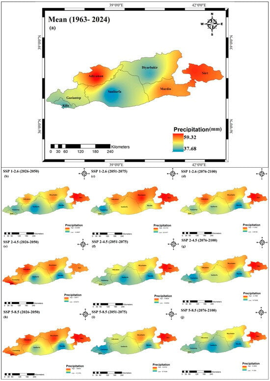
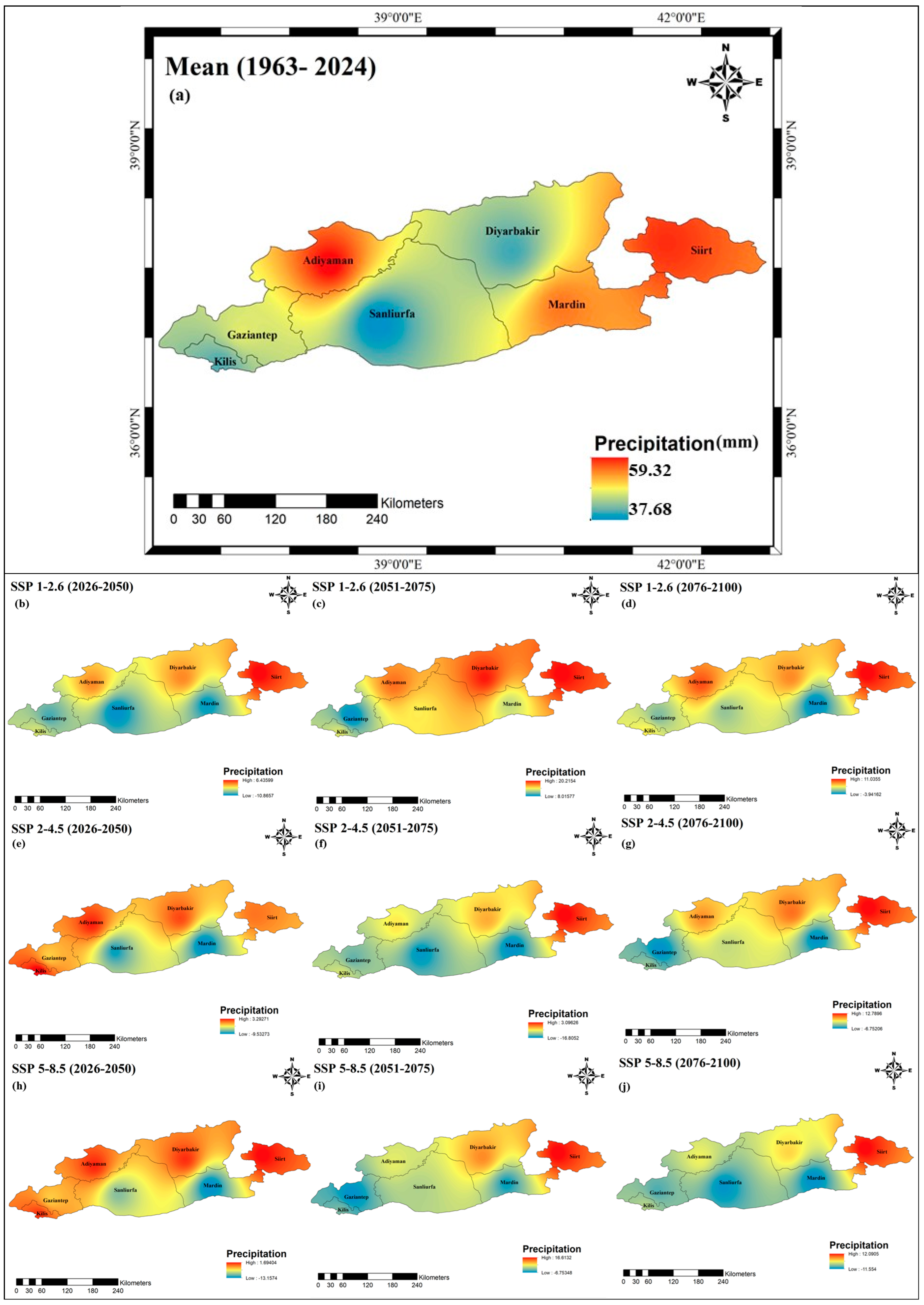
The figure presents a comparative analysis of bias-corrected precipitation projections derived from CMIP6 global climate models for the Southeastern Anatolia Project (GAP) region under the SSP1-2.6 (optimistic), SSP2-4.5 (moderate) and SSP5-8.5 (pessimistic) scenarios (Figure 7). The maps visualize the average rainfall distribution (mm) along with the relative error percentage (RE%) for the three scenarios under different conditions (good, moderate and poor). The first thing that draws attention is the relatively low RE percentages and higher regional coherence observed in the SSP1-2.6 scenario. This shows that prediction errors are reduced in scenarios where climate actions are seriously implemented. While the margins of error remain limited in the northern parts of the GAP region, the increased RE values in the southern and eastern borders indicate that high-resolution local factors can be decisive on projection success. Under the SSP2-4.5 scenario, RE values are moderate, with significant deviations especially along the Şanlıurfa-Mardin line. This indicates that even if current emission trends continue, this may lead to increasing uncertainties in precipitation projections.

Figure 7. Spatial variation in projected PR: (a) baseline (1963–2024); (b–d) relative error (%) for SSP1-2.6 in the near (2026–2050), mid (2051–2075), and far future (2076–2100); (e–g) SSP2-4.5; (h–j) SSP5-8.5.

The most striking results are observed in the SSP5-8.5 scenario, i.e., the high emission case. The maps reveal the situation where both RE rates and inter-projection variance are highest. This scenario represents the condition where model uncertainty and regional climate complexity are most pronounced.

The average precipitation map presented in the bottom panel confirms that the northwestern parts of the region receive relatively higher precipitation, while the southeast is at risk of drought when all projections are considered. This spatial pattern emphasizes that water management policies across the region should be structured to consider local differences.

3.3.2. Average Temperature (Tave)

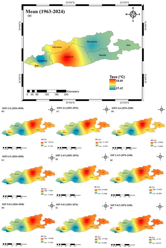
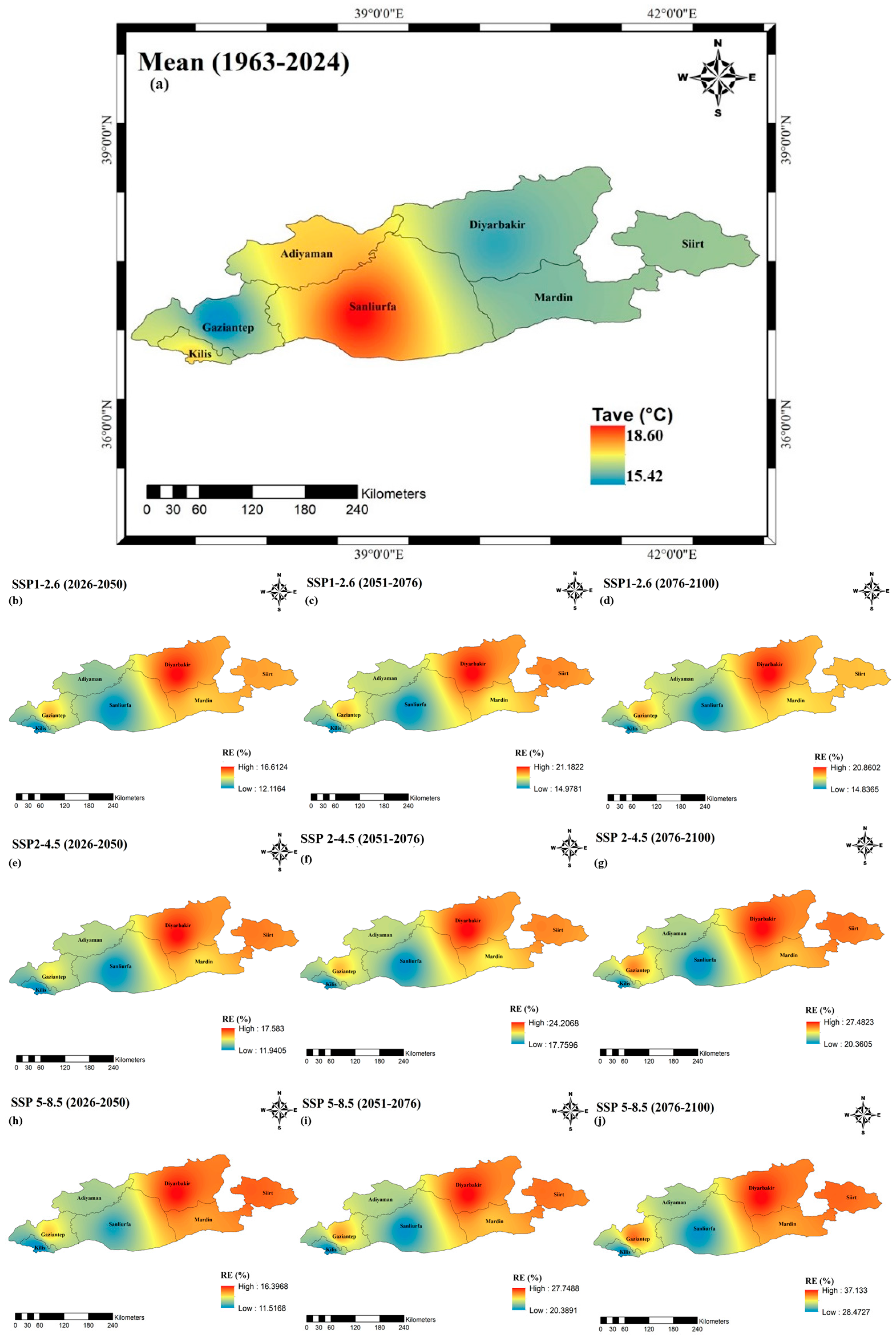
Projections for the GAP region indicate a significant upward trend in temperature for all scenarios and time periods (Figure 8). While the lowest increases are observed in the SSP1-2.6 (sustainable development) scenario, the highest temperature increases occur in the SSP5-8.5 (high emissions) scenario, especially in the period 2076–2100 (far future). When the regional distribution is analysed, it is seen that temperature increases are more pronounced in the northern and central parts of the region. This situation shows that thermal stress will also differentiate spatially due to climate change.

Figure 8. Spatial variation in projected Tave: (a) Baseline (1963–2024); (b–d) relative error (%) for SSP1-2.6 in the near (2026–2050), mid (2051–2075), and far future (2076–2100); (e–g) relative error (%) for SSP2-4.5; and (h–j) relative error (%) for SSP5-8.5.

In the period 2026–2050 (near future), temperature increases under SSP1-2.6 generally remain below +1.5 °C, while values up to +2.5 °C in the SSP5-8.5 scenario are observed. In the far future, the temperature will increase under SSP5-8.5, exceeding +4 °C in some regions. This situation reveals that the region is under serious risk in scenarios where no measures are taken against climate change.

The RE (%) values in the graphs, i.e., the relative error values, show the extent to which the model projections are in line with the observational data. While lower RE values are seen especially in low emission scenarios and in the near future periods, the RE increases in scenarios with high variability such as SSP5-8.5. This shows that the uncertainty of the projections increases with scenario severity.

These findings reveal that warming due to climate change will gradually increase in the GAP region and this will have direct impacts on processes such as agricultural production, water resources and evaporation. Consideration of different scenarios is critical for regional adaptation strategies.

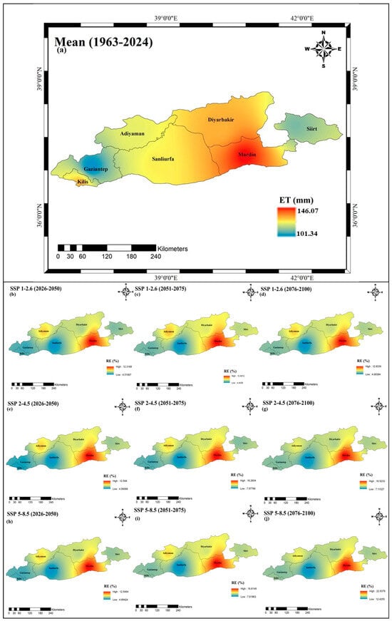
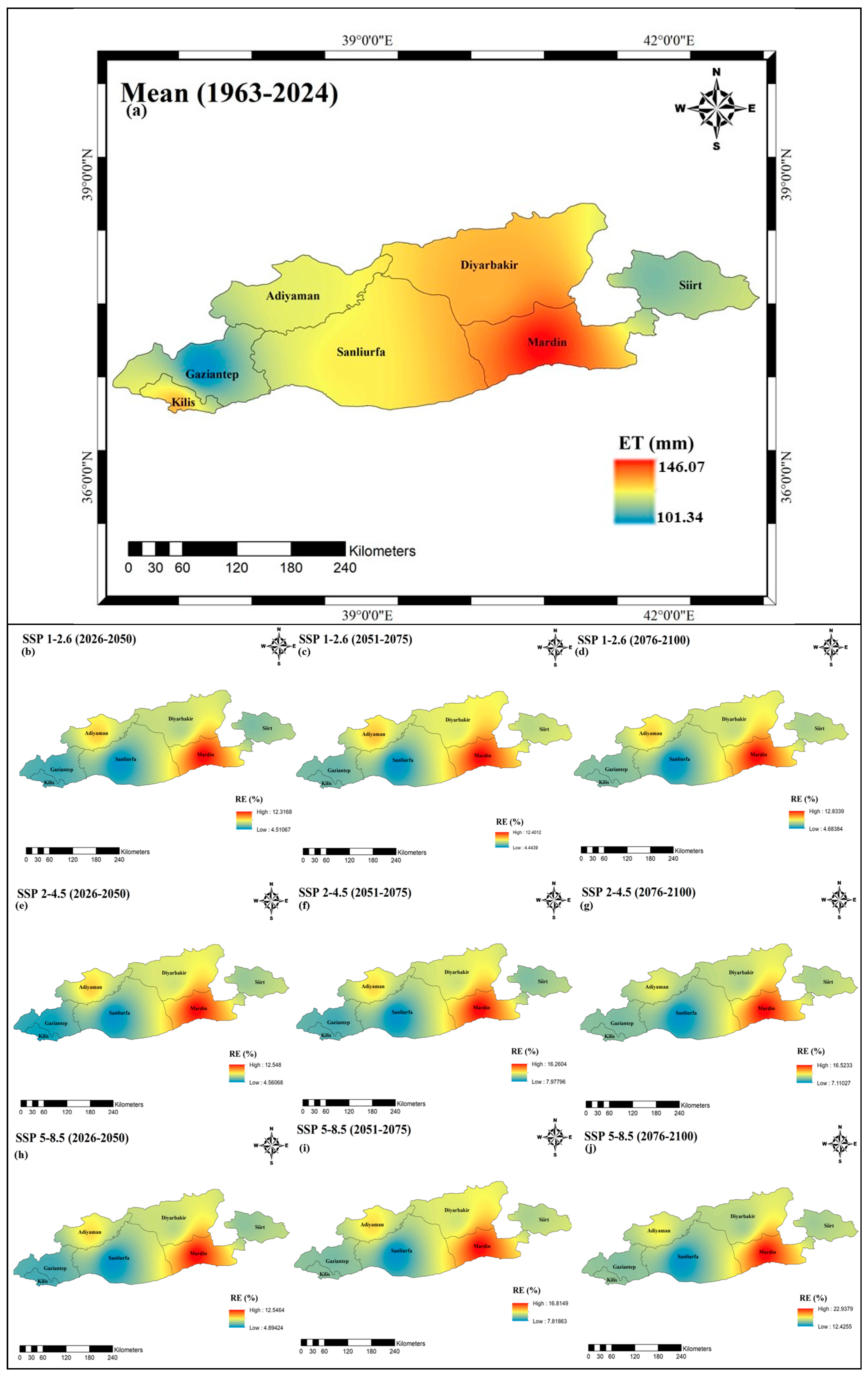
3.3.3. Reference Evapotranspiration (ET0)

Evapotranspiration (ET) projections are an important indicator of the water cycle changes that the region will experience in the face of climate change. Throughout all scenarios and periods, there is an increasing trend in evapotranspiration values in the GAP region (Figure 9). While the increase in ET remains relatively limited in the SSP1-2.6 scenario, this increase becomes evident in the SSP5-8.5 scenario and reaches the highest values especially in the period 2076–2100 (far future). This increase may threaten agricultural production and water management by increasing water losses, which may be even more effective, especially in summer months. When the spatial distribution is analysed, the ET increase is realized at higher levels in the southeast and lowland parts of the region. This indicates that it may lead to more water stress in areas with intensive agricultural activities.

Figure 9. Spatial variation in projected ET: (a) baseline (1963–2024); (b–d) relative error (%) for SSP1-2.6 in the near (2026–2050), mid (2051–2075), and far future (2076–2100); (e–g) SSP2-4.5; (h–j) SSP5-8.5.

Even in the near future (2026–2050), ET values are already showing significant increases in some regions. This trend reveals that the impacts of climate change are already being felt. The average of the scenarios also supports the upward trend in ET values but softens the impact of extreme values somewhat.

The RE (%) values shown on the maps reflect the extent to which model projections are in line with observational data. Generally, RE values are lower in low-emission scenarios. In high–emission scenarios and far future periods, RE increases, indicating an increase in uncertainty. These findings reveal that evaporation and transpiration will increase in the GAP region in the coming years and the pressure on water resources will intensify. This makes the region a priority for both agricultural water management and climate adaptation policies.

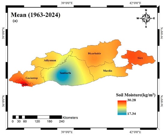
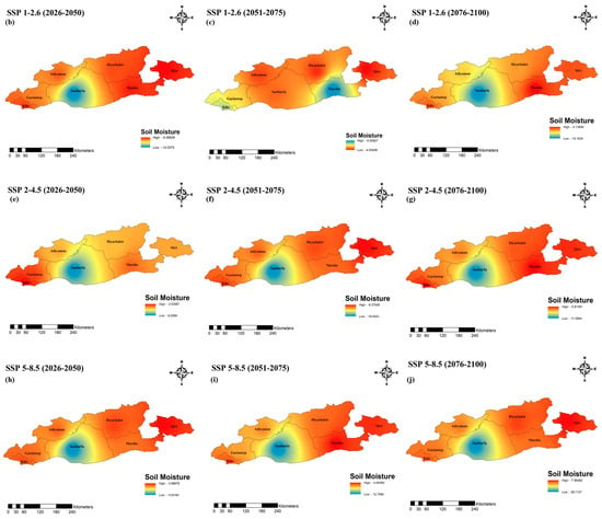
3.3.4. Soil Moisture (SM)

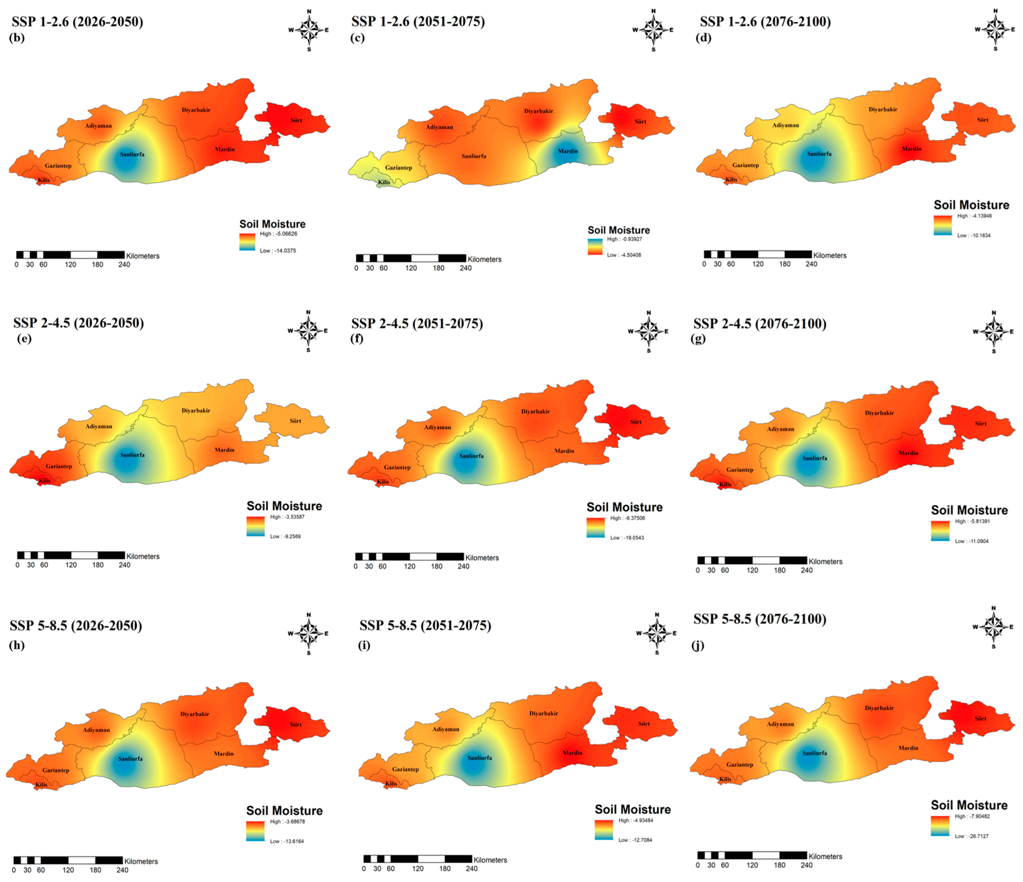
Soil moisture projections are an important indicator that directly reflects the impacts of climate change on both agriculture and the hydrological cycle. The findings of this study reveal that there is a general downward trend in soil moisture in the GAP region in future periods (Figure 10). While relatively constant or limited decreases are observed in some areas under the SSP1-2.6 scenario, this decrease becomes much more pronounced under the SSP5-8.5 scenario. In the period 2076–2100 (far future), soil moisture values decrease significantly in many regions compared to the high emission scenario. This indicates that the risk of drought will increase and productivity in agricultural production may decrease. In terms of spatial distribution, decreases in soil moisture are more intense, especially in the southern and eastern parts. These areas also overlap with regions where evapotranspiration (ET) increases the most, underlining imbalances in the water cycle.

Figure 10. Spatial variation in projected SM: (a) baseline (1963–2024); (b–d) relative error (%) for SSP1-2.6 in the near (2026–2050), mid (2051–2075), and far future (2076–2100); (e–g) SSP2-4.5; (h–j) SSP5-8.5.

In the period 2026–2050, some regions are expected to experience significant declines compared to current conditions. These early impacts show that climate change is already putting significant pressure on water holding capacity. When the average of the scenarios is analysed, extreme fluctuations are somewhat mitigated, but the overall trend is negative. This indicates that uncertainties will become increasingly critical, especially in water-sensitive regions. This downward trend in soil moisture is an important warning for agricultural irrigation management, drought preparedness and ecosystem resilience. Unless region-specific adaptation strategies are developed, the impacts of this trend will be much more pronounced and severe.

4. Discussion

This study’s findings affirm that the Southeastern Anatolia Project (GAP) region is experiencing a distinct climatic alteration, along with global and regional patterns influenced by anthropogenic climate change. The anticipated rises in temperature, evapotranspiration, and the reduction in soil moisture in future periods and emission scenarios highlight the region’s susceptibility to escalating hydroclimatic stress. These findings correspond with extensive evaluations suggesting that arid and semi-arid areas, especially in the Mediterranean and the Middle East, are critical zones for climate change [43,44].

The ongoing warming trend, particularly under SSP5-8.5, along with the corresponding increase in evapotranspiration rates, is anticipated to considerably diminish soil water retention, exerting considerable strain on agricultural systems. Agriculture, the economic foundation of the GAP region, is significantly reliant on irrigation. Elevated temperatures and heightened atmospheric moisture demand may result in diminished crop yields, especially in water-dependent crops like cotton and wheat [34,45]. The anticipated reduction in soil moisture and the rising incidence of drought-like conditions provide a significant danger to food security, rural livelihoods, and economic stability in the region.

Water supplies will encounter increasing pressure from a combination of heightened evapotranspiration, modified precipitation patterns, and diminished effective rainfall. These results corroborate earlier research indicating that climate change will result in reduced streamflow and groundwater recharge in semi-arid basins [46,47]. The GAP region, now facing seasonal water shortages, may experience increased interannual unpredictability and diminished reliability of water availability, especially during the growing season. This directly affects the sustainability of extensive irrigation systems, reservoir management, and transboundary water governance.

Furthermore, the ecosystem services offered by soil moisture and precipitation patterns, including vegetation support, carbon sequestration, and biodiversity preservation, are likely to be compromised. Extended durations of insufficient soil moisture can deteriorate land quality, elevate erosion, and exacerbate the hazards of desertification [48,49]. These ecological alterations may exacerbate socioeconomic vulnerabilities in the region.

The study illustrates the significance of bias correction and downscaling methods in improving the dependability of global climate models for regional decision-making. The application of Quantile Mapping (QM), which demonstrated the highest accuracy when evaluated against empirical data, underscores the imperative of rectifying systemic biases prior to implementing forecasts in vulnerable sectors. The incorporation of a K-Nearest Neighbor weather generator to replicate daily-scale factors like radiation and humidity fills a frequently neglected void in hydrological modeling utilizing CMIP6 datasets [28,39,50].

This work is significant due to its region-specific, multi-variable, and scenario-based examination of climate change effects, which can guide both immediate risk management and long-term adaptation strategies. The GAP region possesses national and geopolitical importance owing to its contributions to agriculture, energy generation, and transboundary river systems. Nevertheless, it continues to be inadequately represented in high-resolution climate effect evaluations. This study addresses a significant knowledge deficiency by generating spatially explicit, bias-corrected forecasts for essential hydroclimatic variables, offering a valuable resource for planners, engineers, and policymakers.

This study indicates that the exacerbation of warming, aridity, and hydrological imbalance in the GAP region underscores the worldwide imperative to enhance local and regional resilience. In the absence of prompt adaptation measures, such as effective irrigation technologies, water recycling methods, crop diversification, and drought early warning systems, the region may encounter significant socio-environmental and economic repercussions in high-emission scenarios [51,52].

5. Conclusions

This study provides a comprehensive spatial and temporal analysis of historical trends and future forecasts for essential hydroclimatic variables (temperature, precipitation, evapotranspiration, and soil moisture) in the Southeastern Anatolia Project (GAP) region of Türkiye. Bias-corrected CMIP6 model outputs were employed across three Shared Socioeconomic Pathways (SSP1-2.6, SSP2-4.5, SSP5-8.5), and the results consistently indicate that the region is experiencing escalating climatic stress, especially under high-emission scenarios. Temperature forecasts suggest a continuous and geographically varied warming trend throughout all future periods, with the most significant rises noted under the SSP5-8.5 scenario in the far future (2076–2100). Significantly, temperature increases over +4 °C are observed in several regions, especially in the northern and central zones. This indicates heightened thermal stress with significant consequences for crop viability, human comfort, and evapotranspiration dynamics.

Evapotranspiration (ET) values demonstrate a persistent upward trajectory across all scenarios and timeframes, underscoring apprehensions about water losses and the increasing demand for irrigation. The southeastern lowland regions, already centers of heavy agricultural production, are particularly susceptible, with forecasts suggesting significant rises in ET in the near future. These alterations indicate a looming water scarcity and the necessity for immediate enhancements in agricultural water management. Soil moisture forecasts indicate a simultaneous and troubling decrease, particularly under the SSP5-8.5 scenario. Reductions in soil water content are most pronounced in the southern and eastern sectors of the GAP region, aligning with zones of heightened evapotranspiration. The simultaneous pressure on the water cycle, resulting from increased evapotranspiration and diminished soil retention, is anticipated to diminish agricultural production and intensify drought susceptibility in the near future. Precipitation forecasts, albeit exhibiting regional heterogeneity, indicate heightened uncertainty under elevated emission scenarios. The relative error (RE) values increase with emission intensity and future time periods, especially near the southern borders and in intricate topographical regions. These uncertainties emphasize the necessity of downscaled and bias-corrected models for regional planning. Precipitation in the northwestern regions remained steady, whilst southeastern areas show declining trends and heightened drought danger.

Historical assessments corroborate the findings by demonstrating a distinct shift over the past sixty years toward a warmer and drier environment, characterized by reduced precipitation, elevated temperatures, heightened evapotranspiration, and declining soil moisture. These alterations affirm that the hydrological equilibrium of the GAP region has been severely disturbed.

The study collectively emphasizes that climate change is not a far issue for the GAP region; it is an immediate and intensifying reality. The synergistic impacts of elevated temperatures, reduced moisture, and hydrological discrepancies pose a significant threat to agriculture, water security, and sustainable development. These insights necessitate immediate, scenario-based adaptation techniques customized to local climate variations and temporal patterns. The findings establish a fundamental scientific foundation for incorporating climate forecasts into water resource management, regional planning, and policy formulation in one of Türkiye’s most vital and climate-sensitive areas.

References

- Kahya, E.; Kalaycı, S. Trend analysis of streamflow in Turkey. J. Hydrol. 2004, 289, 128–144. [Google Scholar] [CrossRef] [Scilit]
- Gumus, B.; Oruc, S.; Yucel, I.; Yilmaz, M.T. Impacts of climate change on extreme climate indices in Türkiye driven by high-resolution downscaled CMIP6 climate models. Sustainability 2023, 15, 7202. [Google Scholar] [CrossRef] [Scilit]
- Maraun, D. Bias correction, quantile mapping, and downscaling: Revisiting the inflation issue. J. Clim. 2013, 26, 2137–2143. [Google Scholar] [CrossRef] [Scilit]
- Teutschbein, C.; Seibert, J. Bias correction of regional climate model simulations for hydrological climate-change impact studies: Review and evaluation of different methods. J. Hydrol. 2012, 456–457, 12–29. [Google Scholar] [CrossRef] [Scilit]
- Gudmundsson, L.; Bremnes, J.; Haugen, J.; Engen-Skaugen, T. Downscaling RCM precipitation to the station scale using statistical transformations—A comparison of methods. Hydrol. Earth Syst. Sci. 2012, 16, 3383–3390. [Google Scholar] [CrossRef] [Scilit]
- Jihan, M.A.T.; Popy, S.; Kayes, S.; Golam, R.; Al Shafi, M.; Mustafijur, R. Climate change scenario in Bangladesh: Historical data analysis and future projection based on CMIP6 model. Sci. Rep. 2025, 15, 7856. [Google Scholar] [CrossRef] [Scilit]
- Doss-Gollin, J.; Keller, K. A subjective Bayesian framework for synthesizing deep uncertainties in climate risk management. Earth’s Future 2023, 11, e2022EF003044. [Google Scholar] [CrossRef] [Scilit]
- Sowjanya, N.P.; Keesara, V.R.; Mesapam, S.; Das, J.; Venkataramana, S. Climate change impacts on streamflow in the Krishna River Basin, India: Uncertainty and multi-site analysis. Climate 2022, 10, 190. [Google Scholar] [CrossRef] [Scilit]
- Kåresdotter, E.; Destouni, G.; Ghajarnia, N.; Lammers, R.B.; Kalantari, Z. Distinguishing direct human-driven effects on the global terrestrial water cycle. Earth’s Future 2022, 10, e2022EF002848. [Google Scholar] [CrossRef] [Scilit]
- Kim, M.K.; Kim, S.; Kim, J.; Heo, J.; Park, J.S.; Kwon, W.T.; Suh, M.S. Statistical downscaling for daily precipitation in Korea using combined PRISM, RCM, and quantile mapping: Part 1, methodology and evaluation in historical simulation. Asia Pac. J. Atmos. Sci. 2016, 52, 79–89. [Google Scholar] [CrossRef] [Scilit]
- Herrera, D.A.; Cook, B.I.; Fasullo, J.; Anchukaitis, K.J.; Alessi, M.; Martinez, C.J.; Evans, C.P.; Li, X.; Ellis, K.N.; Mendez, R.; et al. Observed changes in hydroclimate attributed to human forcing. PLoS Clim. 2023, 3, e0000487. [Google Scholar] [CrossRef] [Scilit]
- Hyndman, D. Evaluating the Impacts of Projected Climate Changes on the Grand Traverse Bay Region, Michigan Sea Grant. 2014. Available online: https://www.michiganseagrant.org/wp-content/uploads/2019/01/Hyndman_Final-IA-Report-20160516_submit.pdf (accessed on 13 November 2025).
- Wang, A.; Miao, Y.; Kong, X.; Wu, H. Future changes in global runoff and runoff coefficient from CMIP6 multi-model simulation under SSP1-2.6 and SSP5-8.5 scenarios. Earth’s Future 2022, 10, e2022EF002910. [Google Scholar] [CrossRef] [Scilit]
- Gebrechorkos, S.H.; Leyland, J.; Dadson, S.J.; Cohen, S.; Slater, L.; Wortmann, M.; Ashworth, P.J.; Bennett, G.L.; Boothroyd, R.; Cloke, H. Global scale evaluation of precipitation datasets for hydrological modelling. Hydrol. Earth Syst. Sci. 2024, 28, 3099–3118. [Google Scholar] [CrossRef] [Scilit]
- Papadimitriou, L.V.; Koutroulis, A.G.; Grillakis, M.G.; Tsanis, I.K. High-end climate change impact on European runoff and low flows–exploring the effects of forcing biases. Hydrol. Earth Syst. Sci. 2016, 20, 1785–1808. [Google Scholar] [CrossRef] [Scilit]
- O’Neill, B.C.; Kriegler, E.; Ebi, K.L.; Kemp-Benedict, E.; Riahi, K.; Rothman, D.S.; Van Ruijven, B.J.; Van Vuuren, D.P.; Birkmann, J.; Kok, K.; et al. The roads ahead: Narratives for shared socioeconomic pathways describing world futures in the 21st century. Glob. Environ. Change 2015, 42, 169–180. [Google Scholar] [CrossRef] [Scilit]
- Riahi, K.; Van Vuuren, D.P.; Kriegler, E.; Edmonds, J.; O’neill, B.C.; Fujimori, S.; Bauer, N.; Calvin, K.; Dellink, R.; Fricko, O.; et al. The Shared Socioeconomic Pathways and their energy, land use, and greenhouse gas emissions implications: An overview. Glob. Environ. Change 2017, 42, 153–168. [Google Scholar] [CrossRef] [Scilit]
- Grose, M.R.; Narsey, S.; Delage, F.P.; Dowdy, A.J.; Bador, M.; Boschat, G.; Chung, C.; Kajtar, J.B.; Rauniyar, S.; Freund, M.B.; et al. Insights from CMIP6 for Australia’s future climate. Earth’s Future 2020, 8, e2019EF001469. [Google Scholar] [CrossRef] [Scilit]
- Wu, T.; Lu, Y.; Fang, Y.; Xin, X.; Li, L.; Li, W.; Jie, W.; Zhang, J.; Liu, Y.; Zhang, L.; et al. The Beijing climate center climate system model (BCC-CSM): The main progress from CMIP5 to CMIP6. Geosci. Model Dev. 2019, 12, 1573–1600. [Google Scholar] [CrossRef] [Scilit]
- Puri, K. The Australian Community Climate and Earth System Simulator, ACCESS: Scientific justification and options for system development. Aust. Meteorol. Oceanogr. J. 2012, 62, 195–210. [Google Scholar] [CrossRef] [Scilit]
- Hausfather, Z.; Drake, H.F.; Abbott, T.; Schmidt, G.A. Evaluating the performance of past climate model projections. Geophys. Res. Lett. 2020, 47, e2019GL085378. [Google Scholar] [CrossRef] [Scilit]
- Nouri, M.; Veysi, S. CMIP6 multi-model ensemble projection of reference evapotranspiration using machine learning algorithms. Agric. Water Manag. 2024, 306, 109190. [Google Scholar] [CrossRef] [Scilit]
- Song, Y.H.; Chung, E.S.; Shahid, S.; Kim, Y.; Kim, D. Development of global monthly dataset of CMIP6 climate variables for estimating evapotranspiration. Sci. Data 2023, 10, 568. [Google Scholar] [CrossRef] [Scilit]
- Engida, T.G.; Muluneh, A.; Zewdie, M. Multi-model ensemble of CMIP6 projections for past and future climate change on mean precipitation and temperature. Environ. Syst. Res. 2025, 14, 28. [Google Scholar] [CrossRef] [Scilit]
- Ojeda, M.G.-V.; Yeste, P.; Gámiz-Fortis, S.R.; Castro-Díez, Y.; Esteban-Parra, M.J. Future changes in land and atmospheric variables: An analysis of their couplings in the Iberian Peninsula. Sci. Total Environ. 2020, 722, 137902. [Google Scholar] [CrossRef] [Scilit]
- Guo, Q.; Chen, J.; Zhang, X.; Shen, M.; Chen, H.; Guo, S. A new two-stage multivariate quantile mapping method for bias correcting climate model outputs. Clim. Dyn. 2019, 53, 3603–3623. [Google Scholar] [CrossRef] [Scilit]
- Allen, R.G.; Pereira, L.S.; Raes, D.; Smith, M. Crop Evapotranspiration: Guidelines for Computing Crop Water Requirements; FAO Irrigation and Drainage Paper 56; FAO: Rome, Italy, 1998; Volume 300, p. D05109. [Google Scholar]
- Sharif, M.; Burn, D.H. Improved K-nearest neighbor weather generating model. J. Hydrol. Eng. 2007, 12, 42–51. [Google Scholar] [CrossRef] [Scilit]
- GAP. What’s GAP? 2021. Available online: http://www.gap.gov.tr/en/ (accessed on 25 June 2025).
- Ozguler, H.; Yıldız, D. Consequences of the droughts in the Euphrates-Tigris Basin. Int. J. Water Manag. Dipl. 2020, 1, 29–40. [Google Scholar]
- Gumus, V.; Simsek, O.; Avsaroglu, Y.; Agun, B. Spatio-temporal trend analysis of drought in the GAP Region, Turkey. Nat. Hazards 2021, 109, 1759–1776. [Google Scholar] [CrossRef] [Scilit]
- Yeşilköy, S.; Şaylan, L. Assessment and modelling of crop yield and water footprint of winter wheat by AquaCrop. Ital. J. Agrometeorol. 2020, 3, 3–14. [Google Scholar] [CrossRef] [Scilit]
- Cannon, A.J.; Sobie, S.R.; Murdock, T.Q. Bias correction of GCM precipitation by quantile mapping: How well do methods preserve changes in quantiles and extremes? J. Clim. 2015, 28, 6938–6959. [Google Scholar] [CrossRef] [Scilit]
- Yeşilköy, S.; Şaylan, L. Yields and water footprints of sunflower and winter wheat under different climate projections. J. Clean. Prod. 2021, 298, 126780. [Google Scholar] [CrossRef] [Scilit]
- Dessu, S.B.; Melesse, A.M. Evaluation and comparison of satellite and GCM rainfall estimates for the Mara River Basin, Kenya/Tanzania. In Climate Change and Water Resources; Springer: Berlin/Heidelberg, Germany, 2013; pp. 29–45. [Google Scholar] [CrossRef] [Scilit]
- Sunyer, M.A.; Madsen, H.; Ang, P.H. A comparison of different regional climate models and statistical downscaling methods for extreme rainfall estimation under climate change. Atmos. Res. 2012, 103, 119–128. [Google Scholar] [CrossRef] [Scilit]
- Kim, K.B.; Kwon, H.; Han, D. Hydrological modelling under climate change considering nonstationarity and seasonal effects. Hydrol. Res. 2016, 47, 260–273. [Google Scholar] [CrossRef] [Scilit]
- Wetterhall, F.; Pappenberger, F.; He, Y.; Freer, J.; Cloke, H.L. Conditioning model output statistics of regional climate model precipitation on circulation patterns. Nonlinear Process. Geophys. 2012, 19, 623–633. [Google Scholar] [CrossRef] [Scilit]
- Yazd, H.R.G.H.; Salehnia, N.; Kolsoumi, S.; Hoogenboom, G. Prediction of climate variables by comparing the k-nearest neighbor method and MIROC5 outputs in an arid environment. Clim. Res. 2019, 77, 99–114. [Google Scholar] [CrossRef] [Scilit]
- Ippolito, M.; De Caro, D.; Cannarozzo, M.; Provenzano, G.; Ciraolo, G. Evaluation of daily crop reference evapotranspiration and sensitivity analysis of FAO Penman-Monteith equation using ERA5-Land reanalysis database in Sicily, Italy. Agric. Water Manag. 2024, 295, 108732. [Google Scholar] [CrossRef] [Scilit]
- Han, Y.; Calabrese, S.; Du, H.; Yin, J. Evaluating biases in Penman and Penman–Monteith evapotranspiration rates at different timescales. J. Hydrol. 2024, 638, 131534. [Google Scholar] [CrossRef] [Scilit]
- Hodam, S.; Sarkar, S.; Marak, A.G.; Bandyopadhyay, A.; Bhadra, A. Spatial interpolation of reference evapotranspiration in India: Comparison of IDW and Kriging methods. J. Inst. Eng. Ser. A 2017, 98, 511–524. [Google Scholar] [CrossRef] [Scilit]
- Giorgi, F.; Lionello, P. Climate change projections for the Mediterranean region. Glob. Planet. Change 2008, 63, 90–104. [Google Scholar] [CrossRef] [Scilit]
- Lelieveld, J.; Proestos, Y.; Hadjinicolaou, P.; Tanarhte, M.; Tyrlis, E.; Zittis, G. Strongly increasing heat extremes in the Middle East and North Africa (MENA) in the 21st century. Clim. Change 2016, 137, 245–260. [Google Scholar] [CrossRef] [Scilit]
- Lobell, D.B.; Schlenker, W.; Costa-Roberts, J. Climate trends and global crop production since 1980. Science 2011, 333, 616–620. [Google Scholar] [CrossRef] [Scilit] [PubMed]
- Vörösmarty, C.J.; McIntyre, P.B.; Gessner, M.O.; Dudgeon, D.; Prusevich, A.; Green, P.; Glidden, S.; Bunn, S.E.; Sullivan, C.A.; Liermann, C.R.; et al. Global threats to human water security and river biodiversity. Nature 2010, 467, 555–561. [Google Scholar] [CrossRef] [Scilit]
- Scanlon, B.R.; Keese, K.E.; Flint, A.L.; Flint, L.E.; Gaye, C.B.; Edmunds, W.M.; Simmers, I. Global synthesis of groundwater recharge in semiarid and arid regions. Hydrol Process 2006, 20, 3335–3370. [Google Scholar] [CrossRef] [Scilit]
- Montanarella, L.; Scholes, R.; Brainich, A. The IPBES Assessment Report on Land Degradation and Restoration; Secretariat of the Intergovernmental Science-Policy Platform on Biodiversity and Ecosystem Services: Bonn, Germany, 2018. [Google Scholar] [CrossRef]
- Huang, J.; Li, Y.; Fu, C.; Chen, F.; Fu, Q.; Dai, A.; Shinoda, M.; Ma, Z.; Guo, W.; Li, Z.; et al. Dryland climate change: Recent progress and challenges. Rev. Geophys. 2017, 55, 719–778. [Google Scholar] [CrossRef] [Scilit]
- Eyring, V.; Bony, S.; Meehl, G.A.; Senior, C.A.; Stevens, B.; Stouffer, R.J.; Taylor, K.E. Overview of the Coupled Model Intercomparison Project Phase 6 (CMIP6) experimental design and organization. Geosci. Model Dev. 2016, 9, 1937–1958. [Google Scholar] [CrossRef] [Scilit]
- Kay, M.; Bunning, S.; Burke, J.; Boerger, V.; Bojic, D.; Bosc, P.M.; Clark, M.; Dale, D.; England, M.; Hoogeveen, J.; et al. The State of the World’s Land and Water Resources for Food and Agriculture 2021. Systems at Breaking Point; Food and Agriculture Organization: Rome, Italy, 2022. [Google Scholar] [CrossRef] [Scilit]
- Intergovernmental Panel on Climate Change (IPCC). Climate Change 2021: The Physical Science Basis; Contribution of Working Group I to the Sixth Assessment Report of the Intergovernmental Panel on Climate Change; Cambridge University Press: Cambridge, UK, 2021. [Google Scholar] [CrossRef] [Scilit]
Disclaimer/Publisher’s Note: The statements, opinions and data contained in all publications are solely those of the individual author(s) and contributor(s) and not of MDPI and/or the editor(s). MDPI and/or the editor(s) disclaim responsibility for any injury to people or property resulting from any ideas, methods, instructions or products referred to in the content. |
© 2026 by the authors. Licensee MDPI, Basel, Switzerland. This article is an open access article distributed under the terms and conditions of the Creative Commons Attribution (CC BY) license.