Integrating Demand/Lead-Time Volatility into a Sustainable Purchasing Portfolio Matrix: A Conceptual Matrix Framework and Empirical Case Study

Abstract

Purchasing portfolio models, particularly the Kraljic matrix, are widely used to support sourcing decisions under supply risk. Yet, they are often criticized for relying on subjective assessments and focusing mainly on upstream uncertainty while neglecting downstream demand volatility. This study develops a quantitatively grounded purchasing portfolio framework that integrates demand volatility and lead-time volatility into a unified measure of supply risk to support more sustainable sourcing decisions. Using transactional data for 876 stock-keeping units (SKUs) from a pharmaceutical distribution company, demand and lead-time volatility are measured through coefficients of variation and combined using an adjusted multifactor model that accounts for their interdependence. Financial importance is measured objectively through gross profit and classified according to the 80–20 Pareto principle. These metrics are incorporated into a revised purchasing portfolio matrix that classifies items into strategic, leverage, bottleneck, and routine categories. The findings reveal substantial variation in combined volatility across SKUs and show that incorporating demand uncertainty significantly changes portfolio positioning compared with traditional approaches. By linking purchasing and marketing perspectives, the proposed model reduces subjectivity, improves risk visibility, and supports sustainable sourcing and inventory decisions in volatile environments.

1. Introduction

In today’s business environment, supply chains operate under high levels of complexity and volatility [1,2]. This volatility constitutes a major source of supply chain risk [3,4] and arises from multiple factors, including fluctuations in exchange rates, raw material prices, stock market volatility, and shipping costs. These factors directly or indirectly influence both demand and lead time, thereby amplifying demand and lead-time volatility [5,6].

Within this volatile context, purchasing plays a strategic role as the primary interface between firms and their upstream supply environment. Purchasing strategies significantly affect firm performance [7] and can generate a sustainable competitive advantage [8,9,10]. As a result, purchasing portfolio models have been widely adopted in both academic research and managerial practice to guide sustainable sourcing decisions and improve competitive positioning [11,12,13]. Beyond strategic benefits, these models also facilitate internal coordination and provide practical guidance for managing heterogeneous purchased items [14,15].

Among these approaches, the Kraljic [16] purchasing portfolio remains the most influential. It classifies purchased items in two dimensions, profit impact and supply risk, resulting in four strategic categories. Subsequent portfolio models largely preserve this two-dimensional logic [17,18,19], differing mainly in how the dimensions are operationalized rather than in their conceptual foundations [20]. Consequently, Kraljic-based portfolio models have been extensively applied across industries [19].

Despite their popularity, purchasing portfolio models, particularly the Kraljic framework, have been widely criticized for their qualitative and subjective nature. Classification decisions often rely on managerial judgment when assigning weights to criteria and positioning items within the matrix [11,12,17,21]. These limitations are commonly summarized as challenges related to the operationalization of dimensions, the measurement of variables, and the determination of clear lines of demarcation [17]. Moreover, existing portfolio models predominantly emphasize upstream supply risks, while largely neglecting downstream sources of uncertainty.

In supply chain management, demand volatility and lead-time volatility represent two interrelated sources of risk with significant implications for operational efficiency and performance [22]. Demand volatility reflects unpredictable fluctuations in customer demand driven by market dynamics and economic conditions [23], often resulting in erratic order patterns, stockouts, or excess inventory. Lead-time volatility, by contrast, introduces uncertainty regarding product availability, making it difficult to synchronize supply capabilities with changing demand and increasing the risk of missed sales and customer dissatisfaction [24]. Their interaction further complicates risk management; demand surges during volatile lead times, increasing stockout risk, while demand declines during extended lead times lead to surplus inventory and higher holding costs [4,25,26].

Traditionally, lead-time volatility has been associated with the purchasing function, which links the firm to its upstream supply environment. In contrast, demand volatility has been viewed as the responsibility of the marketing function, connecting the firm to its downstream market. These functions have often been treated as operating at “the extreme ends of a company’s value process” and largely in isolation from one another [27,28]. Although the emergence of supply chain management in the 1980s emphasized a value chain perspective and highlighted purchasing as a core SCM function [7], purchasing and marketing have continued to evolve in silos, with limited attention to their interdependencies in the literature [28,29,30].

Recognizing purchasing and marketing as two sides of the same value-creation process is critical for effective risk management. Greater coordination between these functions can improve the firm’s ability to jointly manage demand and lead-time volatility, thereby enhancing overall supply chain performance [7]. Addressing this gap, the present study emphasizes the co-management of purchasing and marketing by integrating demand and lead-time volatility into the development of a purchasing portfolio framework. Specifically, the study contributes to reducing the subjectivity inherent in the supply risk dimension of traditional portfolio models by incorporating demand volatility—a downstream risk—alongside lead-time volatility as an upstream risk. In doing so, it proposes a conceptual model that more comprehensively captures supply risk within the purchasing portfolio and strengthens its relevance for managing contemporary supply chain uncertainty. In addition to improving sourcing efficiency, reducing supply uncertainty is increasingly recognized as a sustainability imperative because unstable supply conditions often lead to avoidable waste, emergency transportation, excess safety stocks, and inefficient resource utilization across supply chains [31]. The recent sustainability literature [32,33,34] emphasizes that resilient purchasing decisions simultaneously contribute to economic sustainability, operational continuity, and environmental performance by reducing unnecessary inventory accumulation and minimizing reactive procurement responses during disruption periods.

To address the limitations identified in traditional frameworks, this study adopts a methodological development and empirical validation research design. While prior research [5,21,32,33] has identified various supply chain risk dimensions, this paper introduces a quantitatively grounded framework that operationalizes these risks through an integrated coefficient of variation (CV$) metric. Unlike traditional models that treat purchasing and marketing silos independently, our methodological contribution lies in the mathematical synthesis of downstream demand and upstream supply volatility into a single portfolio coordinate. In addition, while a substantial body of research has sought to refine purchasing portfolio models, most extensions remain anchored in the original logic of the Kraljic framework, particularly in maintaining a clear separation between upstream supply risk and downstream demand conditions. For example, approaches based on multi-criteria decision-making and risk-weighted scoring improve the structure and rigor of classification, but they typically continue to treat demand variability as part of the profit impact or importance dimension rather than as a direct source of supply risk [11,12,32]. At the same time, the more recent supply chain risk management literature highlights that disruptions rarely originate from a single source; instead, risk increasingly emerges from the interaction between supply-side uncertainty and demand-side volatility, particularly in complex and rich data environments [5,22,23]. This systemic view is also increasingly aligned with sustainability-oriented supply chain research, which emphasizes that reducing uncertainty is not only an operational concern but also a sustainability imperative, as volatility-driven inefficiencies often lead to excess inventory, waste, and unnecessary emissions [24,34,35]. Despite this shift in perspective, limited attention has been given to embedding these interactions directly within purchasing portfolio models. In response, this study takes a different approach by explicitly treating demand volatility as a core driver of supply risk and integrating it with lead-time variability into a single, quantitative measure. By doing so, the proposed framework moves beyond the traditional separation of purchasing and marketing considerations and offers a more realistic and sustainability-relevant representation of how risk propagates across the supply chain, thereby providing a stronger analytical basis for sourcing decisions under uncertainty.

The primary objective is to develop a quantitative purchasing portfolio model that integrates downstream demand volatility and validates its utility through an empirical case study. Specifically, this research seeks to answer two core questions:

RQ1: How can demand volatility (downstream) and lead-time volatility (upstream) be mathematically integrated to provide a more objective measure of supply risk?

RQ2: To what extent does this integrated model alter the classification of strategic items compared to a traditional, upstream-only Kraljic matrix?

By applying this model to an empirical case study within the pharmaceutical distribution sector, the study demonstrates a significant shift from qualitative, subjective classification processes toward a data-driven protocol based on historical volatility metrics. This approach not only enhances the precision of item positioning but also strengthens the strategic alignment between a firm’s upstream supply capabilities and its downstream market realities.

Accordingly, this study treats demand volatility as an essential downstream component of supply risk and combines it with lead-time volatility as an upstream indicator. By jointly capturing these two dimensions, the proposed purchasing portfolio framework offers a more comprehensive and operationally relevant representation of supply risk, aligning purchasing strategy with the realities of volatile demand environments.

The remainder of this paper is structured as follows: First, demand and lead-time volatility are reviewed, with particular emphasis on their measurement. The paper then presents a proposed conceptual model that integrates demand and lead-time volatility into an adapted purchasing portfolio. Finally, conclusions and directions for future research are provided.

2. Literature Reviews

The following sections present a literature review of measuring demand and lead-time volatility.

2.1. Demand Volatility

Demand volatility has increased substantially in recent years and is widely regarded as one of the most critical challenges facing contemporary supply chains [6,36]. From a supply chain perspective, demand volatility refers to the variable and unpredictable rate of change in demand, resulting in a lack of stability leading to instability over time [36]. When firms fail to respond effectively to such variability, they face heightened risks of excessive inventory or stockouts, product obsolescence, frequent order expediting, unstable production plans, and increased working capital and variable costs [37,38].

The sources of demand volatility can be broadly classified into natural and artificial drivers, operating at both macro and micro levels. Natural demand volatility at the macro level stems from factors largely beyond managerial control, including competitor behavior, economic and market conditions, industry characteristics, regulatory changes, and disruptive events [4,5,37,39,40,41]. At the micro level, natural drivers include customer ordering behavior, requested order lead times, product life-cycle effects, and seasonality [34,40,41,42,43,44].

Artificial demand volatility, by contrast, arises primarily from managerial and organizational decisions. At the macro level, it is driven by promotional activities, price discounting, trade terms, product variety, new product introductions, supply chain positioning, capacity coordination, and demand planning practices [25,36,45,46]. At the micro level, artificial volatility is closely linked to demand planning processes, including planning horizons, forecasting methods, product aggregation levels, and performance measurement systems [42,47,48,49].

Demand volatility has been conceptualized in the literature using terms such as uncertainty and variability. It has been described as inconsistent or highly variable demand for goods and services [50], uncertainty associated with demand [51], unpredictability in the rate of demand change [37], and variability in customer demand volume and mix [1,52,53]. Practitioners further characterize demand volatility in terms of its degree, frequency, and magnitude of demand fluctuations [54,55]. Collectively, these definitions indicate that demand volatility encompasses both demand uncertainty and demand variability. Accordingly, this study defines demand volatility as a highly variable, inconsistent, and unpredictable rate of change in demand [37,50].

From a measurement perspective, demand volatility is commonly measured by the demand standard deviation [56]. However, the coefficient of variation (CoV)—defined as the standard deviation divided by the mean—has been shown to provide a more robust and comparable measure [57]. As a dimensionless metric, the CoV enables comparison across products, processes, and contexts with differing scales or average demand levels [58]. Despite its widespread use, the literature offers no consensus on threshold values for classifying demand volatility as high or low, as such classifications are highly context-dependent [59,60,61]. Consequently, this study adopts a statistical approach to segmentation by deriving volatility thresholds using a box-and-whisker plot, allowing for data-driven and context-specific classification.

2.2. Lead-Time Volatility

Lead time is a fundamental component of supply chain management, with direct implications for operational efficiency, customer satisfaction, and overall firm performance. It represents the total elapsed time from order placement to delivery, encompassing procurement, production, order processing, and logistics activities [5]. Lead time can be decomposed into internal lead time, associated with a firm’s own processes, and external lead time, which depends on supplier performance and logistics operations [40]. Suppliers that fail to provide reliable lead times are typically perceived as high risk, as lead-time instability increases the likelihood of stockouts, excess inventory, production disruptions, and schedule instability [62].

In recent years, lead-time volatility has increased markedly and has emerged as a critical challenge for supply chains, making its management strategic [36]. Lead-time volatility refers to the variable and unpredictable fluctuations in delivery times that undermine stability and coordination [37,63]. Ineffective management of lead-time variability exposes firms to risks such as excessive inventory or stockouts, production delays, emergency orders, uncertain production schedules, and increased working capital and variable costs [38].

The sources of lead-time volatility can be classified into natural and artificial drivers operating at both macro and micro levels. At the macro level, natural sources include supplier market conditions, geopolitical risks, transportation infrastructure constraints, regulatory changes, and disruptive events [4,5,36,40,41]. At the micro level, natural drivers stem from supplier reliability, production capacity limitations, logistical inefficiencies, and process variability [36,42,43,45].

Artificial lead-time volatility, by contrast, arises from managerial and organizational decisions. At the macro level, it is influenced by supply chain strategies, supplier selection policies, outsourcing decisions, and inventory management practices [25,36,45,46]. At the micro level, artificial volatility is driven by order batching, inefficient internal processes, poor information sharing, and a lack of coordination across functions and partners [42,47,48,49].

As supply chains become more complex and interconnected, managing lead-time volatility increasingly depends on advanced technological capabilities. Internal factors such as production capacity and process efficiency continue to shape order completion times. At the same time, external influences, including supplier reliability, transportation constraints, and geopolitical disruptions, remain significant sources of variability [25]. Recent advances in artificial intelligence and machine learning support real-time forecasting and predictive analytics, enabling firms to anticipate and mitigate lead-time disruptions [64]. Similarly, Industry 4.0 technologies, including IoT-enabled systems, enhance visibility and coordination across supply chain partners [59]. Together, these developments underscore the importance of data-driven, proactive approaches to lead-time management in volatile environments.

For methodological consistency, this study measures lead-time volatility using the coefficient of variation (CoV), consistent with the approach applied to demand volatility. This ensures comparability across upstream and downstream dimensions of variability and supports their joint integration into the supply risk construct within the proposed purchasing portfolio framework.

3. Conceptual Model

To ensure the reliability and replicability of the proposed conceptual model, the study followed a four-stage data preparation protocol designed to transform raw transactional records into standardized risk metrics. First, Data Cleaning, including handling the missing data, was performed to remove statistical outliers in both demand and lead-time datasets, defined as values exceeding three standard deviations from the mean. Second, Normalization was achieved by converting the raw units to the coefficient of variation. This step is essential to ensure that dimensions are scale-invariant, allowing for a meaningful comparison between high-volume and low-volume items. Third, Correlation Testing was conducted by computing the Pearson correlation coefficient for each SKU category to identify the degree of interdependence between upstream and downstream volatility. Finally, the Integration stage involved applying the combined volatility formula to generate a unified supply risk coordinate, which serves as the quantitative basis for positioning items within the final purchasing portfolio matrix.

The proposed purchasing portfolio matrix will be created using data sourced from a pharmaceutical distribution retail company’s internal databases and documents that encompass 876 SKUs during the year 2023. The pharmaceutical distributor investigated can be categorized as part of the retail sector, specifically under the subcategory of wholesale or distribution in the subcategory of the pharmaceutical industry. Pharmaceutical distributors serve as intermediaries between manufacturers and healthcare providers, including pharmacies, hospitals, and clinics. While they primarily engage in wholesale distribution of medications and medical supplies, their role is essential to the overall retail landscape of pharmaceuticals, as they ensure products are delivered to end users effectively.

The development process of the proposed matrix will unfold in three sequential stages:

• Establishing Supply Risk: In the first stage, the supply risk dimension will be determined by assessing the combined volatility of demand volatility and lead-time volatility.
• Assessing Financial Importance: The second stage will focus on identifying the financial significance of each item using the 80-20 Pareto rule, measured by gross margin (or gross profit). This metric represents the difference between sales revenues and the Cost of Goods Sold (COGS), which includes the landed costs associated with the goods for retail companies.
• Integrating Metrics: In the final stage, the financial metrics will be integrated with the supply risk dimension established in the first stage. This integration will facilitate the development of portfolio quadrants, culminating in a comprehensive portfolio model specifically tailored for pharmaceutical firms.

3.1. First Stage: Calculating Combined Volatility

In the first stage of developing the purchasing portfolio matrix, it is essential to calculate the individual volatilities of demand and lead time for each SKU as shown in Table 1.

Table 1. Combined volatility (partial output).

SKU (pn)	Avg Demand	Demand Standard Deviation	Demand/Volatility	Avg. Lead-Time/Days	Lead-Time Std Dev	Lead-Time Volatility	Volatility	Supply Risk
SKU #131	294,079.20	263,441.84	0.90	18.25	15.43	0.85	1.22	N
SKU #309	193,888.40	532,824.55	2.75	50.83	0.41	0.01	2.75	N
SKU #80	185,997.99	227,399.66	1.22	62.17	19.03	0.31	1.25	L
SKU #449	8867.88	18,078.00	2.04	66.50	12.79	0.19	2.04	M
SKU #668	50,204.78	99,727.47	1.99	18.62	13.49	0.72	2.10	H
SKU #830	168.47	583.61	3.46	70.40	24.83	0.35	3.47	M
SKU #817	92,516.67	261,401.52	2.83	16.56	2.60	0.16	2.83	H
SKU #236	302,752.48	629,542.04	2.08	68.50	18.58	0.27	2.09	N
SKU #439	36,357.96	66,468.90	1.83	64.00	8.49	0.13	1.83	L
SKU #671	125,538.72	246,092.30	1.96	131.83	68.07	0.52	2.01	L
SKU #706	96,742.84	335,127.03	3.46	52.80	25.65	0.49	3.48	M
SKU #217	130,747.00	321,552.78	2.46	43.50	17.69	0.41	2.48	M
SKU #13	17,072.14	56,107.84	3.29	47.25	24.17	0.51	3.31	H
SKU #339	308,168.71	260,839.41	0.85	17.50	9.26	0.53	0.99	N
SKU #719	89,001.03	307,228.82	3.45	60.50	25.32	0.42	3.47	L
SKU #123	494,742.97	470,328.11	0.95	47.00	4.24	0.09	0.95	L
SKU #312	8894.16	13,747.38	1.55	19.00	14.56	0.77	1.71	N

Given the interdependence between demand and lead-time volatility, it is critical to calculate a combined volatility metric that integrates both demand volatility and lead-time volatility. By doing so, organizations can gain a clearer understanding of their supply chain’s risk profile. For instance, the interplay between these two forms of volatility significantly impacts suppliers, who must adjust production schedules and inventory levels in response to erratic demand patterns. The high lead-time volatility can exacerbate challenges faced by suppliers, making it difficult for them to accommodate sudden changes in order quantities.

To effectively manage these compounded risks, an adjusted multifactor model can be employed to quantify the combined volatility. Rather than averaging the two volatilities, the model accounts for their relationship. The combined volatility is derived from the statistical property of the sum of two random variables:

$${\sigma }_C=\sqrt{{(\sigma }_D^2+{\sigma }_L^{2 })+(2{\rho }_{DL}{\sigma }_D{\sigma }_L)}$$

Variable Definitions

• Let represent ${\sigma }_D$ demand volatility (coefficient of variation of demand).
• Let ${\sigma }_L$ represent lead-time volatility (coefficient of variation of lead time).
• Let ${\rho }_{DL}$ represent the Pearson correlation coefficient between demand and lead time.
• Let ${\sigma }_C$ represent the Combined Supply Risk Volatility.

The use of the combined volatility formula is rooted in probability theory, specifically the variance of the sum of dependent variables. While the empirical correlation (${\rho }_{DL}$) in this case study is low and marginally significant, the inclusion of the covariance term ($2{\rho }_{DL}{\sigma }_D{\sigma }_L$) is methodologically necessary to ensure the model’s universal applicability.

Even when ${\rho }_{DL}$ ≈ 0, the formula remains robust, as it simplifies toward the Pythagorean sum of independent risks $(\sqrt{{\sigma }_D^2+{\sigma }_L^2}$). Retaining the correlation term keeps the portfolio model sensitive to “worst-case” scenarios in which demand surges coincide with supply delays (positive correlation) and “buffer” scenarios (negative correlation).

This approach not only reflects the individual risks associated with demand and lead time but also captures their interdependence, allowing for more informed decision-making in purchasing and inventory management. Ultimately, developing this combined volatility measure is a foundational step towards enhancing supply chain risk management, fostering resilience, and enabling organizations to respond more effectively to fluctuations in demand and supply availability. Notably, the correlation between demand and lead-time volatility was negative (−0.027) and statistically significant (p-value = 0.053), which is less than the alpha level of 0.1. This indicates that as demand volatility increases, lead-time volatility tends to decrease, highlighting the complexity of managing these interconnected risks.

In traditional supply chain models, a positive correlation often exists between demand volatility and lead-time volatility, typically exacerbated by the Bullwhip Effect [65]. When customer demand is stable, suppliers can effectively plan their production and logistics, resulting in consistent lead times. Conversely, when demand spikes, suppliers face capacity constraints, leading to production backlogs and erratic lead times. However, the observed negative correlation in some cases highlights the possibility of a strategic operational setup where suppliers actively counterbalance changes in demand volatility with controlled lead-time variability. This occurs when suppliers prioritize high-demand customers (Highly Valued Customers, or HVCs) by absorbing demand variability through dedicated sustainable resources and inventory buffers. Consequently, a sharp increase in demand can result in stable and low lead-time volatility as the supplier makes extraordinary efforts to meet customer needs.

The observed near-zero to negative correlation in this study is not merely a statistical artifact but is deeply rooted in the strategic operational protocols reported by the case company. Qualitative evidence from the firm confirms that this decoupling between downstream demand and upstream supply results from deliberate “strategic buffering” and supplier prioritization.

According to the company’s procurement leadership, this negative correlation is achieved through three specific mechanisms:

• Priority Safety-Stocking: For High-Value Categories (HVCs), the company mandates that suppliers maintain elevated safety-stock levels. This ensures that unexpected demand spikes are fulfilled immediately from inventory, preventing the volatility from “bleeding into” the delivery lead time.
• Dedicated Capacity Allocation: The case company utilizes formal agreements to secure dedicated production lines. This allows suppliers to respond swiftly to fluctuations in order volume while stabilizing lead times, effectively neutralizing the impact of demand surges on supply velocity.
• Strategic Logistics Consolidation: Conversely, in scenarios where demand is predictably low or non-urgent, the company permits suppliers to consolidate orders to optimize transport efficiency. This operational choice intentionally increases lead-time variability to achieve lower logistics costs, illustrating how lead-time volatility is used as a strategic lever for cost management.

These documented strategies provide a clear empirical basis for the observed negative correlation. By fostering these specific supplier behaviors, the case company effectively utilizes lead-time flexibility to absorb demand uncertainty, reinforcing the stability of its most critical product flows. Accordingly, the combined volatility for each SKU is calculated and shown in Table 1.

Furthermore, a cut-off point is used to categorize combined volatility based on a box-and-whisker plot. Therefore, a coefficient of variation less than the first quartile is considered negligible (N) combined volatility, while the one that is greater than or equal to the first quartile and less than the median is considered low (L) combined volatility. In addition, a coefficient of variation greater than or equal to the median and less than the third quartile is moderate (M) combined volatility, while a coefficient of variation greater than or equal to the third quartile is high (H) combined volatility, as shown in Table 2. Accordingly, the categorization results of combined volatility are shown in Table 1 and will be referred to as “Supply Risk”.

Table 2. Combined volatility categorization scale.

Variable	Q1	Median	Q3
Coefficient	1.8815	2.16695	3.4628
Scale of Categorization	Negligible (N) < Q1	Q1 ≤ Low (L) < Median	Median ≤ Moderate (M) < Q3	High (H) ≥ Q3

The data in Table 1 reveal that, in most cases, the standard deviation of demand for the pharmaceutical company investigated is higher than the average demand, indicating a significant level of variability in demand patterns. This high variability can stem from various factors, including seasonal trends, consumer preferences, economic conditions, new product introductions, and external influences such as economic downturns or natural disasters. In industries marked by high seasonality or rapid innovation, such fluctuations are often normal. Additionally, the product life cycle can affect demand volatility, with new products typically exhibiting greater variability than established ones. Therefore, benchmarking these metrics against industry standards is essential, highlighting the need for adaptive strategies to navigate uncertainty.

For this pharmaceutical distributor, the observation suggests that demand is particularly unpredictable, influenced by factors unique to the industry. Seasonal fluctuations in illness, regulatory changes, and new medication introductions can cause substantial shifts in demand. This unpredictability poses challenges in maintaining optimal inventory levels and ensuring timely supply to healthcare providers, especially during health crises or epidemics. Consequently, pharmaceutical distributors must adopt flexible planning and responsive strategies to manage their inventory and distribution needs effectively. Relying solely on average demand risks stockouts of critical medications or excess inventory of less in-demand products, adversely affecting patient care and profitability. Moreover, strict regulatory requirements further complicate demand forecasting, making it crucial for the distributor to understand demand variability and align strategies accordingly to optimize operational efficiency and serve healthcare providers effectively.

3.2. Second Stage

Maximizing profit is the main goal for businesses, which is the key to the long-term survival and growth of any private organization [62]. For businesses, the profitability of the products they offer, among other factors, largely affects the firm’s profitability. Thus, firms need to accurately measure their products’ profitability, as this enables them to develop effective strategies for management, marketing, production, and operation, and those strategies eventually help companies increase their profits [64]. Studies revealed that the most profitable 20% of the products generate more than 150% of profits and 50% of turnover [66], which reveals the importance of calculating product profitability. Accountants use different measures of profit, including gross margin, contribution margin, and net profit. Gross margin (so-called gross profit) is the difference between sales revenues and the Cost of Goods Sold (COGS). COGS differs across business types; for retail companies, it represents the landed costs.

The gross profit for each SKU is derived by subtracting the COGS from the total revenue generated by sales. This calculation serves as a critical indicator of a product’s financial performance, as it reveals the portion of revenue remaining after covering the direct costs associated with producing or purchasing the goods. Each SKU’s gross profit is calculated individually, allowing for an effective comparison based on profitability as shown in Table 3.

Table 3. SKU gross profit (partial output).

SKU (pn)	Cost of Goods Sold	Revenue	Gross Profit	Profit %	Cumulative Profit %	Combined Volatility	Supply Risk
SKU #131	622,539.337	739,192.950	116,653.614	2.965%	2.965%	1.2152	N
SKU #775	529,402.160	621,721.798	92,319.637	2.346%	5.311%	2.7479	M
SKU #309	525,136.349	610,604.154	85,467.805	2.172%	7.483%	1.2523	N
SKU #386	441,489.444	522,017.721	80,528.277	2.047%	9.529%	2.0425	L
SKU #40	418,638.942	494,877.389	76,238.448	1.937%	11.467%	2.0960	L
SKU #102	391,168.071	461,523.585	70,355.514	1.788%	13.255%	3.4725	H
SKU #449	389,898.696	456,551.556	66,652.860	1.694%	14.949%	2.8256	M
SKU #34	388,489.692	453,936.812	65,447.120	1.663%	16.612%	2.0897	L
SKU #1396	320,949.216	381,082.685	60,133.469	1.528%	18.140%	1.8294	N
SKU #256	314,901.630	371,611.988	56,710.358	1.441%	19.581%	2.0136	L
SKU #688	277,713.473	332,634.665	54,921.191	1.396%	20.977%	3.4850	H
SKU #223	262,838.485	314,240.023	51,401.539	1.306%	22.283%	2.4819	M
SKU #830	257,714.844	308,922.400	51,207.556	1.301%	23.585%	3.3124	M
SKU #135	247,675.163	296,369.290	48,694.126	1.237%	24.822%	0.9859	N
SKU #817	226,891.912	272,593.503	45,701.591	1.161%	25.984%	3.4660	H
SKU #166	226,873.609	272,282.870	45,409.261	1.154%	27.138%	0.9525	N
SKU #236	208,524.234	253,894.965	45,370.731	1.153%	28.291%	1.7066	N
SKU #108	203,784.530	247,374.960	43,590.430	1.108%	29.399%	2.1184	L
SKU #439	195,453.428	235,621.960	40,168.532	1.021%	30.419%	1.4830	N
SKU #324	193,112.118	233,243.614	40,131.495	1.020%	31.439%	3.4766	H
SKU #671	189,651.925	229,658.722	40,006.797	1.017%	32.456%	1.9015	L
SKU #436	186,069.949	225,432.104	39,362.156	1.000%	33.456%	1.6838	N
SKU #706	175,358.858	212,148.008	36,789.150	0.935%	34.391%	2.4775	M
SKU #103	169,630.643	206,032.032	36,401.389	0.925%	35.316%	2.1921	L
SKU #217	169,486.105	205,849.115	36,363.010	0.924%	36.240%	2.7124	M
SKU #288	167,779.842	203,529.195	35,749.353	0.909%	37.149%	1.5861	N
SKU #13	167,069.324	201,759.779	34,690.456	0.882%	38.031%	3.4668	H
SKU #21	165,088.188	199,721.938	34,633.750	0.880%	38.911%	2.8102	M
SKU #111	165,015.000	198,746.685	33,731.685	0.857%	39.768%	1.5275	N
SKU #1385	163,680.519	197,188.537	33,508.018	0.852%	40.620%	2.2407	L

To apply the 80-20 Pareto rule, the initial calculations involve sorting SKUs in descending order by gross profit. This arrangement allows immediate identification of which products contribute most to overall profitability. SKU, with the highest gross profit, naturally leads this list, reflecting not only a substantial dollar amount but also a favorable profit margin, meaning a greater return on each dollar of revenue generated as shown in Table 3.

As the analysis of the organized SKU list progresses, a noticeable decrease in gross profit and profit margins emerges. This pattern indicates that a smaller number of products account for the majority of profits, consistent with the Pareto principle. To gain a clearer understanding of the overall financial impact, the cumulative profit percentage is calculated, progressively summing the profits from the leading SKUs. This method highlights how a relatively small subset of SKUs often contributes significantly to the total profits, underscoring the 80-20 rule, as illustrated in Table 3, which integrates combined volatility and supply risk.

By pinpointing these strategic SKUs, businesses can concentrate on optimizing their inventory and marketing strategies for the most profitable items, facilitating more effective and sustainable resource allocation and enhancing overall financial performance.

3.3. Third Stage

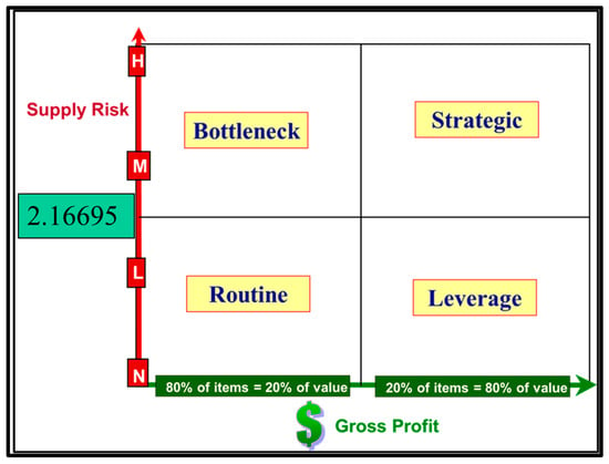
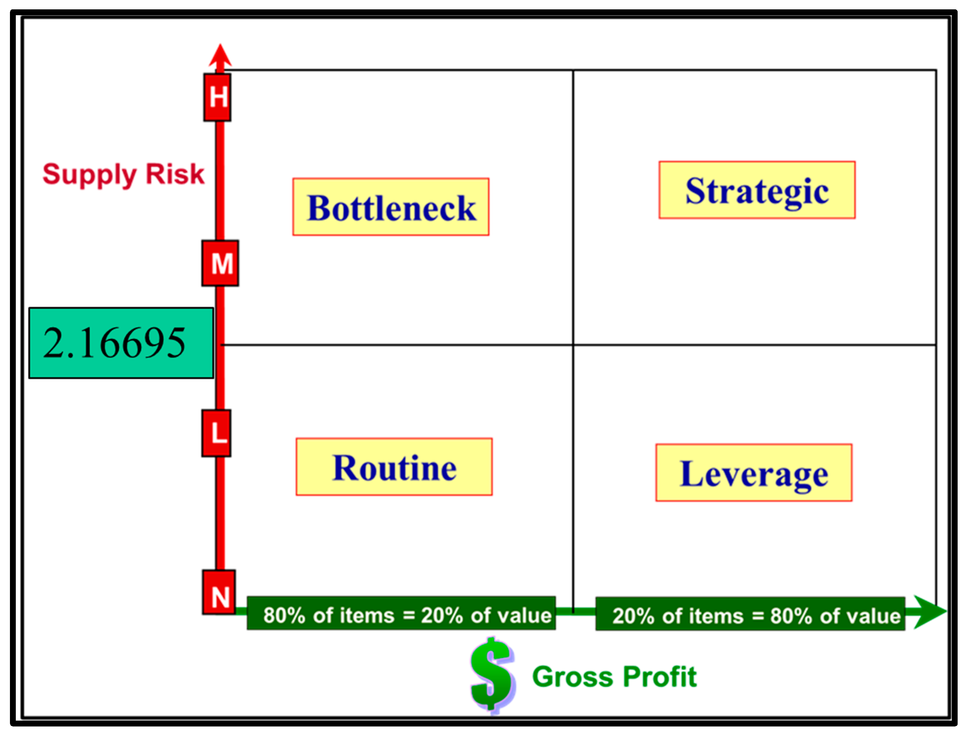
The third stage focuses on developing a purchasing portfolio matrix that categorizes purchased products by two factors: profit impact and supply risk (both low and high). This creates a 2 × 2 matrix that classifies items into four categories: bottleneck, non-strategic, leverage, and strategic items. The profit impact will be divided into two scales based on the 80-20 Pareto analysis, represented on the x-axis, as shown in Figure 1. The y-axis, which represents supply risk, will be split into two regions to delineate the quadrants, as illustrated in Figure 1.

Figure 1. Framework of the purchasing portfolio matrix: profit impact vs. supply risk.

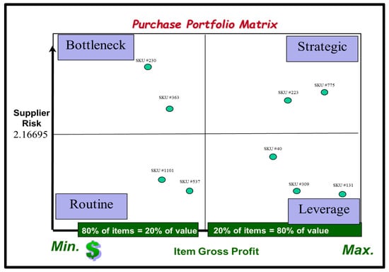
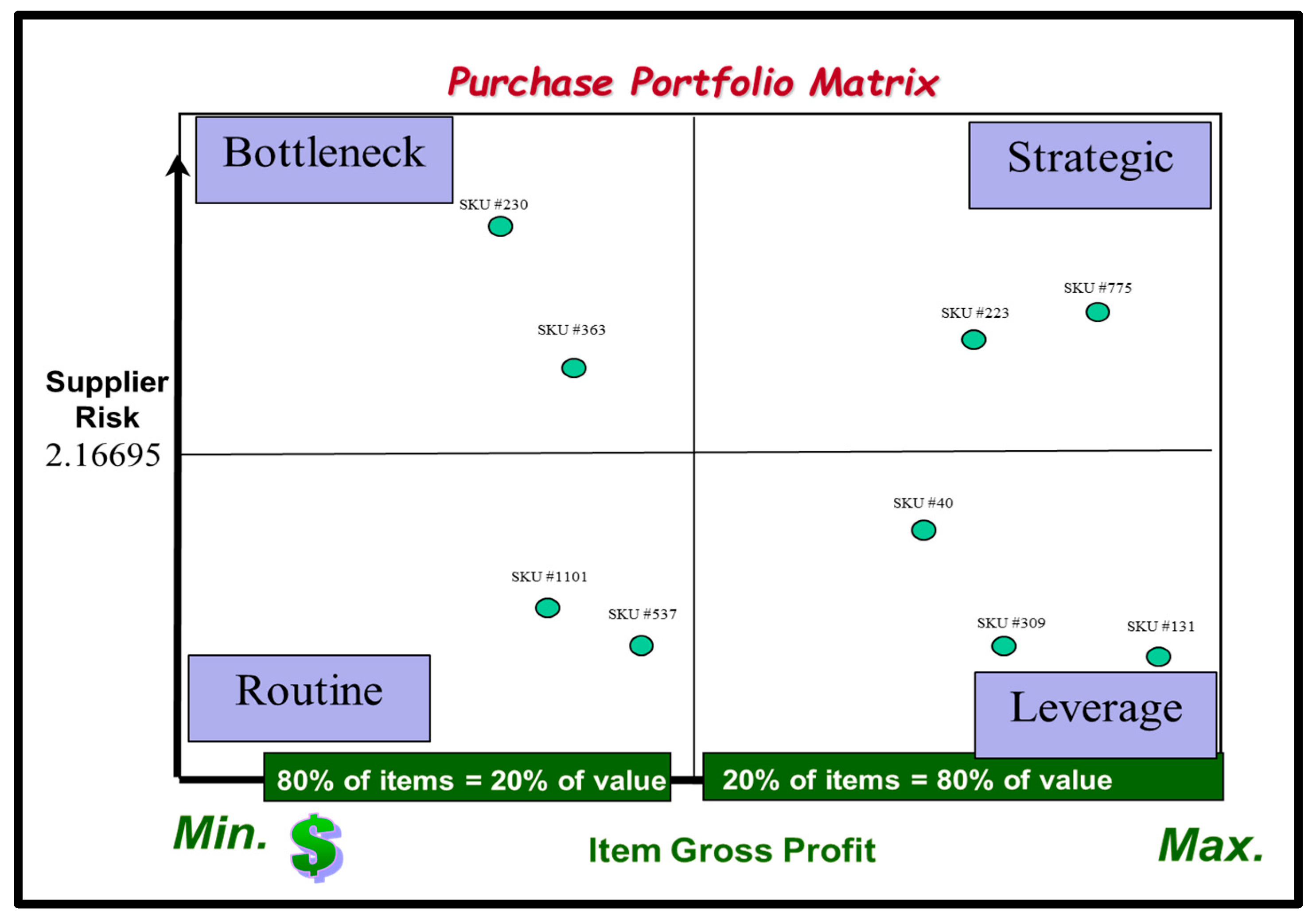
For illustrative purposes, the matrix will report the 20% items and 80% items separately. For the 20% items, any SKU with a supply risk score below 2.16695 will fall into the Leverage quadrant, while those with a score above 2.16695 will fall into the Strategic quadrant as shown in Table 4. For 80% of the items, any SKU with a supply risk score below 2.16695 will fall into the Routine quadrant, while those with a score above 2.16695 will fall into the Bottleneck quadrant as shown in Table 5. Finally, the results of Table 4 and Table 5 can be plotted as shown in Figure 2.

Table 4. Twenty percent of SKUs fall into Leverage and Strategic quadrants (partial output).

SKU (pn)	Cost of Goods Sold	Revenue	Gross Profit	Profit %	Cumulative Profit %	Combined Volatility	Supply Risk	Quadrant
SKU #131	622,539	739,193	116,654	0.0296	2.96%	1.2152	N	Leverage
SKU #775	529,402	621,722	92,320	0.0235	5.31%	2.7479	M	Strategic
SKU #309	525,136	610,604	85,468	0.0217	7.48%	1.2523	N	Leverage
SKU #386	441,489	522,018	80,528	0.0205	9.53%	2.0425	L	Leverage
SKU #40	418,639	494,877	76,238	0.0194	11.46%	2.0960	L	Leverage
SKU #102	391,168	461,524	70,356	0.0179	13.25%	3.4725	H	Strategic
SKU #449	389,899	456,552	66,653	0.0169	14.94%	2.8256	M	Strategic
SKU #34	388,490	453,937	65,447	0.0166	16.61%	2.0897	L	Leverage
SKU #1396	320,949	381,083	60,133	0.0153	18.14%	1.8294	N	Leverage
SKU #256	314,902	371,612	56,710	0.0144	19.58%	2.0136	L	Leverage
SKU #688	277,713	332,635	54,921	0.0140	20.97%	3.4850	H	Strategic
SKU #223	262,838	314,240	51,402	0.0131	22.28%	2.4819	M	Strategic
SKU #830	257,715	308,922	51,208	0.0130	23.58%	3.3124	M	Strategic
SKU #135	247,675	296,369	48,694	0.0124	24.82%	0.9859	N	Leverage
SKU #817	226,892	272,594	45,702	0.0116	25.98%	3.4660	H	Strategic
SKU #166	226,874	272,283	45,409	0.0115	27.13%	0.9525	N	Leverage
SKU #236	208,524	253,895	45,371	0.0115	28.28%	1.7066	N	Leverage
SKU #108	203,785	247,375	43,590	0.0111	29.39%	2.1184	L	Leverage
SKU #439	195,453	235,622	40,169	0.0102	30.41%	1.4830	N	Leverage
SKU #324	193,112	233,244	40,131	0.0102	31.43%	3.4766	H	Strategic
SKU #671	189,652	229,659	40,007	0.0102	32.45%	1.9015	L	Leverage
SKU #436	186,070	225,432	39,362	0.0100	33.45%	1.6838	N	Leverage
SKU #706	175,359	212,148	36,789	0.0093	34.38%	2.4775	M	Strategic
SKU #103	169,631	206,032	36,401	0.0092	35.31%	2.1921	M	Strategic
SKU #217	169,486	205,849	36,363	0.0092	36.23%	2.7124	M	Strategic
SKU #288	167,780	203,529	35,749	0.0091	37.14%	1.5861	N	Leverage
SKU #13	167,069	201,760	34,690	0.0088	38.02%	3.4668	H	Strategic
SKU #21	165,088	199,722	34,634	0.0088	38.90%	2.8102	M	Strategic
SKU #111	165,015	198,747	33,732	0.0086	39.76%	1.5275	N	Leverage
SKU #1385	163,681	197,189	33,508	0.0085	40.61%	2.2407	M	Strategic
SKU #339	158,414	191,759	33,345	0.0085	41.46%	2.5504	M	Strategic
SKU #600	156,295	189,249	32,954	0.0084	42.29%	3.4714	H	Strategic
SKU #719	151,579	184,386	32,807	0.0083	43.13%	2.2606	M	Strategic
SKU #462	149,901	181,022	31,121	0.0079	43.92%	2.0372	L	Leverage

Table 5. Eighty percent of SKUs fall into Routine and Bottleneck quadrants (partial output).

SKU (pn)	Cost of Goods Sold	Revenue	Gross Profit	Profit %	Cumulative Profit %	Combined Volatility	Supply Risk	Quadrant
SKU #537	21,119	25,541	4423	0.0011	81.07%	1.6819	N	Routine
SKU #363	20,961	25,355	4394	0.0011	81.19%	2.3348	M	Bottleneck
SKU #1101	20,921	25,311	4390	0.0011	81.30%	1.5086	N	Routine
SKU #1390	20,881	25,228	4348	0.0011	81.41%	2.3450	M	Bottleneck
SKU #540	20,851	25,118	4267	0.0011	81.52%	3.4676	H	Bottleneck
SKU #829	20,782	25,018	4236	0.0011	81.62%	3.3625	M	Bottleneck
SKU #95	20,720	24,876	4156	0.0011	81.73%	3.0611	M	Bottleneck
SKU #185	20,646	24,782	4136	0.0011	81.83%	1.0843	N	Routine
SKU #230	20,510	24,646	4135	0.0011	81.94%	3.4640	H	Bottleneck
SKU #274	20,397	24,523	4127	0.0010	82.04%	1.1514	N	Routine
SKU #365	20,103	24,176	4072	0.0010	82.15%	1.3501	N	Routine
SKU #1188	20,051	24,108	4057	0.0010	82.25%	3.4173	M	Bottleneck
SKU #1530	19,950	23,999	4049	0.0010	82.35%	2.9061	M	Bottleneck
SKU #190	19,691	23,724	4032	0.0010	82.46%	1.9389	L	Routine
SKU #319	19,521	23,470	3948	0.0010	82.56%	1.5741	N	Routine
SKU #725	19,455	23,397	3942	0.0010	82.66%	1.5166	N	Routine
SKU #1525	19,450	23,391	3941	0.0010	82.76%	2.3379	M	Bottleneck
SKU #516	19,395	23,237	3841	0.0010	82.85%	1.2964	N	Routine
SKU #1109	19,272	23,101	3829	0.0010	82.95%	1.3902	N	Routine
SKU #53	19,090	22,913	3823	0.0010	83.05%	1.4941	N	Routine
SKU #599	19,077	22,898	3821	0.0010	83.15%	3.4633	H	Bottleneck
SKU #399	18,904	22,713	3808	0.0010	83.24%	1.5727	N	Routine
SKU #42	18,602	22,406	3804	0.0010	83.34%	1.8970	L	Routine
SKU #1413	18,563	22,348	3785	0.0010	83.44%	1.4594	N	Routine
SKU #1471	18,532	22,313	3780	0.0010	83.53%	1.7028	N	Routine
SKU #1483	18,457	22,229	3773	0.0010	83.63%	1.8560	N	Routine
SKU #598	17,997	21,766	3769	0.0010	83.72%	2.4855	M	Bottleneck
SKU #26	17,839	21,581	3742	0.0010	83.82%	1.5437	N	Routine
SKU #1482	17,836	21,568	3732	0.0009	83.91%	3.2049	M	Bottleneck
SKU #1093	17,772	21,484	3712	0.0009	84.01%	2.3913	M	Bottleneck
SKU #379	17,618	21,299	3681	0.0009	84.10%	1.4583	N	Routine
SKU #360	17,516	21,164	3649	0.0009	84.19%	1.7058	N	Routine
SKU #1138	17,462	21,100	3638	0.0009	84.29%	1.6162	N	Routine
SKU #1326	17,454	21,066	3611	0.0009	84.38%	1.8639	N	Routine

Figure 2. Illustrative plotting of SKUs.

3.4. Comparative Analysis and Evidence of Portfolio Reclassification

While the Kraljic Matrix [16] remains the foundational benchmark for purchasing strategies, it traditionally defines “Supply Risk” through external market complexities, such as supplier scarcity, entry barriers, or geographical distance. This established upstream-centric perspective frequently treats risk as a static attribute of the external supply market. Our study, however, positions itself at the intersection of the purchasing portfolio management (PPM) and Supply Chain Integration (SCI) literature. We contend that supply risk is not solely an external market condition, but an endogenous variable generated by the interaction between upstream lead-time instability and downstream demand volatility. By pivoting the focus from “market complexity” to “integrated flow uncertainty,” our framework addresses a critical blind spot in the extant literature: the tendency for stable lead times to mask high-exposure risks.

The fundamental distinction between our framework and prior approaches [11,12,32] lies in the mathematical synthesis of risk dimensions. While the existing literature typically relegates demand fluctuations to “Profit Impact” or “Importance of Purchase,” our model re-categorizes demand volatility as a primary driver of supply risk. This shift is theoretically grounded in the premise that an item’s strategic importance is dictated by the probability of stockouts—a state determined by the variance in both supply and consumption. By introducing the Combined Volatility Index, we move away from the siloed, qualitative assessments of traditional models toward a dynamic, quantitative demarcation of risk that accounts for the compounding effects of uncertainty across the entire value chain.

The necessity of this theoretical repositioning is confirmed by our comparative analysis of SKU reclassifications. As illustrated in Table 6, relying exclusively on upstream lead-time volatility—the traditional metric for supply risk—results in the significant misclassification of strategic items.

Table 6. Comparative impact of integrating demand volatility.

SKU (pn)	Upstream Risk (Lead-Time Volatility)	Downstream Risk (Demand Volatility)	Combined Volatility	Revised Supply Risk Category	Strategic Shift
SKU #312	0.77	1.55	1.71	Negligible (N)	Remains Low Priority
SKU #668	0.72	1.99	2.10	High (H)	Shift to High Risk
SKU #309	0.01	2.75	2.75	Negligible (N)	Stable Buffering
SKU #123	0.09	0.95	0.95	Low (L)	Shift to Active Monitoring
SKU #131	0.85	0.90	1.22	Negligible (N)	Baseline
SKU #13	0.51	3.29	3.31	High (H)	Major Shift to Strategic

• Evidence of Misclassification: SKU #312 and SKU #668 possess nearly identical upstream volatility (0.77 and 0.72). Under a traditional Kraljic model, both would share a similar position on the supply risk axis as they belong to the same spending category (where 20% of items account for 80% of expenditure).
• The Impact of Integration: Once downstream demand volatility is integrated, SKU #668 is reclassified as high risk (H) due to its substantial demand fluctuations (1.99), while SKU #312 remains negligible (N).
• Pronounced Shifts: This effect is even more acute in items like SKU #13, which exhibits moderate lead-time uncertainty (0.51) but extreme demand volatility (3.29). The resulting combined volatility (3.31) elevates this item to the high-risk category.

These reclassifications provide systematic evidence that our integrated model captures “hidden” risks ignored by siloed purchasing frameworks. By accounting for the mathematical interaction between upstream and downstream uncertainties, the model offers a more robust demarcation of risk. This ensures that managers do not mislabel high-volatility items as “non-strategic” simply because their lead times appear stable. Ultimately, this contribution strengthens the paper by providing both practitioners and scholars with a method to detect risks that traditional, upstream-only frameworks are mathematically incapable of identifying.

4. Conclusions

The conceptual model presented in the research offers a quantified framework for the traditional Kraljic purchasing portfolio matrix by integrating market-facing demand dynamics with upstream supply risk. It addresses the criticism of subjectivity in the “Purchase Importance” dimension by replacing it with a measurable financial metric: gross profit (or profit contribution). This dimension is segmented based on the 80-20 Pareto rule, identifying high-value items (20% of SKUs generating 80% of value) and low-value items (80% of SKUs generating 20% of value).

The research’s central contribution is the integration of demand volatility and lead-time volatility to create a comprehensive, quantified measure of supply risk [67]. Demand volatility, which is linked to the marketing function, and lead-time volatility, which is linked to the purchasing function, are both measured using the coefficient of variation (CoV) for consistent comparison. An adjusted multifactor model is then used to calculate a combined volatility metric that explicitly accounts for the correlation between these two forms of uncertainty. This combined volatility is then categorized (negligible, low, moderate, high) using a box-and-whisker statistical plot to establish the cut-off points for the supply risk axis of the portfolio matrix.

This resulting portfolio matrix effectively categorizes purchased items into four strategic quadrants: Strategic, Leverage, Bottleneck, and Routine (or Non-Strategic), based on their position relative to the gross profit (profit impact) and the combined volatility (supply risk) cut-off points. The use of these quantifiable, integrated metrics provides practitioners with a robust framework for proposing targeted action plans related to both purchasing and marketing functions, facilitating the co-management of these historically siloed areas to create superior value and enhance overall supply chain performance. From a sustainability perspective, the proposed framework also supports more responsible inventory and sourcing decisions by better aligning procurement behavior with actual market requirements. More accurate identification of volatility-sensitive items can reduce overstocking, stock obsolescence, emergency replenishment, and unnecessary logistics interventions, all of which carry environmental and economic costs [68].

While the framework achieves its primary objective of integrating demand dynamics and providing quantitative rigor and sustainability, the study acknowledges its limitations and identifies avenues for future research. Specifically, it highlights the need to address the supplier’s risk dimensions more fully and to develop detailed action plans for each of the four resulting quadrants. Future work should also consider integrating a broader array of costs, such as manufacturing, administrative, logistics, and fixed costs, into the gross profit dimension to further refine the financial importance metric within the Kraljic model.

References

- Tachizawa, E.M.; Thomsen, C.G. Drivers and sources of supply flexibility: An exploratory study. Int. J. Oper. Prod. Manag. 2007, 27, 1115–1136. [Google Scholar] [CrossRef] [Scilit]
- Mishra, D.; Muduli, K.; Raut, R.; Narkhede, B.E.; Shee, H.; Jana, S.K. Challenges facing artificial intelligence adoption during COVID-19 pandemic: An investigation into the agriculture and agri-food supply chain in India. Sustainability 2023, 15, 6377. [Google Scholar] [CrossRef] [Scilit]
- Christopher, M.; Holweg, M. Supply Chain 2.0: Managing supply chains in the era of turbulence. Int. J. Phys. Distrib. Logist. Manag. 2011, 41, 63–82. [Google Scholar] [CrossRef] [Scilit]
- Wang, J.; Li, Y.; Chen, G. Modeling and analyzing supply chain reliability under uncertainty: A simulation-based study using real-world data. Iraqi Acad. Sci. J. 2024; in press.
- Christopher, M.; Holweg, M. Supply chain 2.0 revisited: A framework for managing volatility induced risk in the supply chain. Int. J. Phys. Distrib. Logist. Manag. 2017, 47, 2–17. [Google Scholar] [CrossRef] [Scilit]
- Anguzu, R.; Aila, F. Sources of supply chain volatility: A literature review. Int. J. Supply Chain Manag. 2024, 9, 20–36. [Google Scholar] [CrossRef] [Scilit]
- Padhi, S.S.; Wagner, S.M.; Aggarwal, V. Positioning of commodities using the Kraljic portfolio matrix. J. Purch. Supply Manag. 2012, 18, 1–8. [Google Scholar] [CrossRef] [Scilit]
- Ellram, L.M.; Carr, A.S. Strategic purchasing: A history and review of the literature. Int. J. Purch. Mater. Manag. 1994, 30, 10–19. [Google Scholar] [CrossRef] [Scilit]
- Carter, J.R.; Narasimhan, R. Is purchasing really strategic? Int. J. Purch. Mater. Manag. 1996, 32, 20–28. [Google Scholar] [CrossRef] [Scilit]
- Chen, I.J.; Paulraj, A.; Lado, A.A. Strategic purchasing, supply management, and firm performance. J. Oper. Manag. 2004, 22, 505–523. [Google Scholar] [CrossRef] [Scilit]
- Knight, L.; Tu, Y.-H.; Preston, J. Integrating skills profiling and purchasing portfolio management: An opportunity for building purchasing capability. Int. J. Prod. Econ. 2014, 147, 271–283. [Google Scholar] [CrossRef] [Scilit]
- Gelderman, C.J.; Van Weele, A.J. Handling measurement issues and strategic directions in Kraljic’s purchasing portfolio model. J. Purch. Supply Manag. 2003, 9, 207–216. [Google Scholar] [CrossRef] [Scilit]
- Wynstra, F.; Ten Pierick, E. Managing supplier involvement in new product development: A portfolio approach. Eur. J. Purch. Supply Manag. 2000, 6, 49–57. [Google Scholar] [CrossRef] [Scilit]
- Dubois, A.; Pedersen, A.C. Why relationships do not fit into purchasing portfolio models: A comparison between the portfolio and industrial network approaches. Eur. J. Purch. Supply Manag. 2002, 8, 35–42. [Google Scholar] [CrossRef] [Scilit]
- Gelderman, C.J.; Semeijn, J. Managing the global supply base through purchasing portfolio management. J. Purch. Supply Manag. 2006, 12, 209–217. [Google Scholar] [CrossRef] [Scilit]
- Kraljic, P. Purchasing must become supply management. Harv. Bus. Rev. 1983, 61, 109–117. [Google Scholar]
- Olsen, R.F.; Ellram, L.M. A portfolio approach to supplier relationships. Ind. Mark. Manag. 1997, 26, 101–113. [Google Scholar] [CrossRef] [Scilit]
- Bensaou, M. Portfolios of buyer-supplier relationships. MIT Sloan Manag. Rev. 1999, 40, 35–44. [Google Scholar]
- Lee, D.M.; Drake, P.R. A portfolio model for component purchasing strategy and the case study of two South Korean elevator manufacturers. Int. J. Prod. Res. 2010, 48, 6651–6682. [Google Scholar] [CrossRef] [Scilit]
- Hadeler, B.J.; Evans, J.R. Supply strategy: Capturing the value. Ind. Manag. 1994, 36, 3–8. [Google Scholar]
- Mohammad, A.S.; Razmi, J.; Ghorbani, M. Classify purchasing items based on risk and profitability attributes using MCDM and FMEA techniques. Res. J. Int. Stud. 2011, 21, 80–85. [Google Scholar]
- Nitsche, B.; Straube, F. Efficiently managing supply chain volatility: A management framework for the manufacturing industry. Procedia Manuf. 2020, 43, 320–327. [Google Scholar] [CrossRef] [Scilit]
- Tao, J.; Aamir, M.; Shoaib, M.; Yasir, N.; Babar, M. Bridging the gap between supply chain risk and organizational performance conditioning to demand uncertainty. Sustainability 2025, 17, 2462. [Google Scholar] [CrossRef] [Scilit]
- Li, Z.; Fei, W.; Zhou, E.; Gajpal, Y.; Chen, X. The impact of lead time uncertainty on supply chain performance considering carbon cost. Sustainability 2019, 11, 6457. [Google Scholar] [CrossRef] [Scilit]
- Hendricks, K.B.; Singhal, V.R. The effect of demand–supply mismatches on firm risk. Prod. Oper. Manag. 2014, 23, 2137–2151. [Google Scholar] [CrossRef] [Scilit]
- Dey, B.K.; Bhuniya, S.; Sarkar, B. Involvement of controllable lead time and variable demand for a smart manufacturing system under a supply chain management. Expert Syst. Appl. 2021, 184, 115464. [Google Scholar] [CrossRef] [Scilit]
- Ivens, B.S.; Pardo, C.; Tunisini, A. Organizing and integrating marketing and purchasing in business markets: An introduction to the special issue, issues and implications. Ind. Mark. Manag. 2009, 38, 851–856. [Google Scholar] [CrossRef] [Scilit]
- Sheth, J.N.; Sharma, A.; Iyer, G.R. Why integrating purchasing with marketing is both inevitable and beneficial. Ind. Mark. Manag. 2009, 38, 865–871. [Google Scholar] [CrossRef] [Scilit]
- Smirnova, M.; Henneberg, S.C.; Ashnai, B.; Naudé, P.; Mouzas, S. Understanding the role of marketing–purchasing collaboration in industrial markets: The case of Russia. Ind. Mark. Manag. 2011, 40, 54–64. [Google Scholar] [CrossRef] [Scilit]
- Gonzalez-Zapatero, C.; Gonzalez-Benito, J.; Lannelongue, G. Antecedents of functional integration during new product development: The purchasing–marketing link. Ind. Mark. Manag. 2016, 52, 47–59. [Google Scholar] [CrossRef] [Scilit]
- Tang, C.S. Perspectives in supply chain risk management. Int. J. Prod. Econ. 2006, 103, 451–488. [Google Scholar] [CrossRef] [Scilit]
- Yalcin, A.S.; Kilic, H.S.; Cevikcan, E. A novel strategy segmentation methodology integrating Kraljic portfolio matrix and supplier relationship model: A case study from machinery industry. Benchmarking 2024, 31, 3587–3623. [Google Scholar] [CrossRef] [Scilit]
- Mirzaee, H.; Ashtab, S. Sustainability, resiliency, and artificial intelligence in supplier selection: A triple-themed review. Sustainability 2024, 16, 8325. [Google Scholar] [CrossRef] [Scilit]
- Becerra, P.; Mula, J.; Sanchis, R. Green supply chain quantitative models for sustainable inventory management: A review. J. Clean. Prod. 2021, 328, 129544. [Google Scholar] [CrossRef] [Scilit]
- Holloway, S. The role of inventory management in achieving sustainability in supply chains. Preprints.org 2024. [Google Scholar] [CrossRef] [Scilit]
- Packowski, J. Lean Supply Chain Planning: The New Supply Chain Management Paradigm for Process Industries to Master Today’s VUCA World; CRC Press: Boca Raton, FL, USA, 2014. [Google Scholar]
- El-Sakty, K.G.; Osama, E. Improving supply chain performance using “VUCA” drivers. J. Supply Chain Manag. Res. Pract. 2015, 9, 1–10. [Google Scholar]
- Song, Y.; Hu, X. Learning-based demand-supply-coupled charging station location problem for electric vehicle demand management. Transp. Res. Part D Transp. Environ. 2023, 125, 103975. [Google Scholar] [CrossRef] [Scilit]
- Rensburg, D.J.J.; Pretorius, L. Managing for volatility on technology projects: A conceptual model. Procedia Soc. Behav. Sci. 2014, 110, 40–51. [Google Scholar] [CrossRef] [Scilit]
- Chopra, S.; Meindl, P. Supply Chain Management: Strategy, Planning, and Operation, 3rd ed.; Pearson Prentice Hall: Upper Saddle River, NJ, USA, 2007. [Google Scholar]
- Chan, H.K.; Lettice, F.; Durowoju, O.A. Decision-Making for Supply Chain Integration; Springer: Berlin/Heidelberg, Germany, 2012. [Google Scholar]
- Stadtler, H.; Kilger, C.; Meyr, H. Supply Chain Management and Advanced Planning, 5th ed.; Springer: Berlin/Heidelberg, Germany, 2015. [Google Scholar]
- Alicke, K.; Forsting, M. McKinsey supply chain segmentation framework. In Supply Chain Segmentation; Springer: Cham, Switzerland, 2015; pp. 15–26. [Google Scholar] [CrossRef] [Scilit]
- Kaufman, P.J. Trading Systems and Methods, 5th ed.; John Wiley & Sons: Hoboken, NJ, USA, 2013. [Google Scholar]
- Chase, C.W. Next Generation Demand Management: People, Process, Analytics, and Technology; John Wiley & Sons: Hoboken, NJ, USA, 2016. [Google Scholar]
- Potter, A.; Towill, D.R.; Christopher, M. Evolution of the migratory supply chain model. Supply Chain Manag. 2015, 20, 603–612. [Google Scholar] [CrossRef] [Scilit]
- Kilger, C.; Wagner, M. Demand planning. In Supply Chain Management and Advanced Planning, 5th ed.; Stadtler, H., Kilger, C., Meyr, H., Eds.; Springer: Berlin/Heidelberg, Germany, 2015; pp. 125–154. [Google Scholar]
- Zotteri, G.; Kalchschmidt, M.; Caniato, F. The impact of aggregation level on forecasting performance. Int. J. Prod. Econ. 2005, 94, 479–491. [Google Scholar] [CrossRef] [Scilit]
- Shcherbakov, M.V.; Brebels, A.; Shcherbakova, N.L.; Tyukov, A.P.; Janovsky, T.A.; Kamaev, V.A. A survey of forecast error measures. World Appl. Sci. J. 2013, 24, 171–176. [Google Scholar]
- Saldanha, T.J.V.; Melville, N.P.; Ramirez, R.; Richardson, V.J. Information systems for collaborating versus transacting: Impact on manufacturing plant performance in the presence of demand volatility. J. Oper. Manag. 2013, 31, 313–329. [Google Scholar] [CrossRef] [Scilit]
- Celly, K.S.; Frazier, G.L. Outcome-based and behavior-based coordination efforts in channel relationships. J. Mark. Res. 1996, 33, 200–210. [Google Scholar] [CrossRef] [Scilit]
- Lee, H.L. Aligning supply chain strategies with product uncertainties. Calif. Manag. Rev. 2002, 44, 105–119. [Google Scholar] [CrossRef] [Scilit]
- Pujawan, N. Assessing supply chain flexibility: A conceptual framework and a case study. Int. J. Integr. Supply Manag. 2004, 1, 79–97. [Google Scholar] [CrossRef] [Scilit]
- Hashemi, A.; Butcher, T.; Chhetri, P. A modeling framework for the analysis of supply chain complexity using product design and demand characteristics. J. Supply Chain Manag. Syst. 2013, 5, 150–164. [Google Scholar] [CrossRef] [Scilit]
- Mason-Jones, R.; Naylor, B.; Towill, D.R. Engineering the leagile supply chain. Int. J. Agile Manag. Syst. 2000, 2, 54–61. [Google Scholar] [CrossRef] [Scilit]
- Panik, M.J. Statistical Inference: A Short Course; John Wiley & Sons: Hoboken, NJ, USA, 2012. [Google Scholar]
- Gilliland, M. The Business Forecasting Deal; John Wiley & Sons: Hoboken, NJ, USA, 2010. [Google Scholar] [CrossRef] [Scilit]
- Asimow, L.A.; Maxwell, M.M. Probability and Statistics with Applications: A Problem Solving Text; ACTEX Publications: Winsted, MN, USA, 2010. [Google Scholar]
- Scholz-Reiter, B.; Heger, J.; Meinecke, C.; Bergmann, J. Integration of demand forecasts in ABC-XYZ analysis: Practical investigation at an industrial company. Int. J. Product. Perform. Manag. 2012, 61, 445–451. [Google Scholar] [CrossRef] [Scilit]
- Forstner, L.; Mönch, L. A heuristic to support make-to-stock, assemble-to-order, and make-to-order decisions in semiconductor supply chains. In Proceedings of the Winter Simulation Conference, Washington, DC, USA, 8–11 December 2013; pp. 3696–3706. [Google Scholar] [CrossRef] [Scilit]
- Engelmeyer, T. Managing Intermittent Demand; Springer: Wiesbaden, Germany, 2016. [Google Scholar]
- Pittman, P.; Atwater, B. Supply uncertainty is the risk of disruption in the flow of components from upstream suppliers. Supply Chain Manag. Rev. 2022, 26, 1–6. [Google Scholar]
- Ahmed Zainul Abideen, F.; Mohamad, F.B. Supply chain lead time reduction in a pharmaceutical production warehouse: A case study. Int. J. Pharm. Healthc. Mark. 2020, 14, 61–88. [Google Scholar] [CrossRef] [Scilit]
- Choi, P. Constructing a balanced view of profit structure in grocery retailing: A field illustration using accounting profits and anchor category profits. Manag. Res. Rev. 2017, 40, 726–744. [Google Scholar] [CrossRef] [Scilit]
- Brauch, M.; Mohaghegh, M.; Größler, A. Causes of the bullwhip effect: A systematic review and categorization of its causes. Manag. Res. Rev. 2024, 47, 1127–1149. [Google Scholar] [CrossRef] [Scilit]
- Noone, B.; Griffin, P. Enhancing yield management with customer profitability analysis. Int. J. Contemp. Hosp. Manag. 1997, 9, 75–79. [Google Scholar] [CrossRef] [Scilit]
- Luo, G.; Liu, X.; Chan, F.T.S. Optimal ordering decisions in portfolio procurement considering spot price fluctuation. Sustainability 2023, 15, 11169. [Google Scholar] [CrossRef] [Scilit]
- Han, N.; Um, J. Risk management strategy for supply chain sustainability and resilience capability. Risk Manag. 2024, 26, 6. [Google Scholar] [CrossRef] [Scilit]
Disclaimer/Publisher’s Note: The statements, opinions and data contained in all publications are solely those of the individual author(s) and contributor(s) and not of MDPI and/or the editor(s). MDPI and/or the editor(s) disclaim responsibility for any injury to people or property resulting from any ideas, methods, instructions or products referred to in the content. |
© 2026 by the authors. Licensee MDPI, Basel, Switzerland. This article is an open access article distributed under the terms and conditions of the Creative Commons Attribution (CC BY) license.