Hybrid Temporal Convolutional Networks and Long Short-Term Memory Model for Accurate and Sustainable Wind–Solar Power Forecasting Leveraging Time-Frequency Joint Analysis and Multi-Head Self-Attention

Abstract

Accurate forecasting of wind and photovoltaic power remains challenging due to the strong nonlinearity, nonstationarity, and seasonal heterogeneity of renewable generation series. To address this issue, this study proposes a hybrid forecasting framework integrating time–frequency joint analysis (TFAA), temporal convolutional networks (TCN), long short-term memory (LSTM), and multi-head self-attention (MHSA). Wavelet transform is used to extract frequency-domain representations, which are jointly encoded with the original time-domain sequence through a dual-branch architecture and adaptively fused. The fused features are then processed by a TCN-LSTM backbone to capture both long-range dependencies and short-term dynamics, while MHSA is introduced to enhance global contextual modeling. Experiments on wind-farm and photovoltaic datasets from China, together with external validation on the NREL WIND Toolkit and the GEFCom2014 Solar benchmark, show that the proposed model achieves the best overall seasonal performance and maintains competitive improvements on public benchmarks. Additional ablation studies, repeated-run statistical validation, persistence-based skill-score analysis, prediction-interval evaluation, ramp-event assessment, meteorological-driver enrichment, permutation-based driver attribution, regime-conditioned error diagnostics, and transferability evidence analysis further confirm the effectiveness, robustness, physical consistency, and practical applicability of the proposed framework. The results indicate that the proposed model provides a reliable and operationally relevant solution for short-term wind and photovoltaic power forecasting. These findings further support sustainable renewable-energy integration, smart-grid dispatch, and low-carbon power-system operation.

1. Introduction

Wind and solar power have emerged as essential components in the global transition to renewable energy, offering critical solutions to climate change and energy crises. However, their generation is highly dependent on meteorological conditions, making them inherently volatile and intermittent. This variability poses substantial challenges for the stable and secure operation of power grids, particularly when these sources are integrated on a large scale. Fluctuations in generation can result in grid frequency deviations, voltage instability, and other operational issues. Therefore, accurate forecasting of wind and solar power generation is crucial for optimizing power system scheduling and energy management. Precise forecasts can reduce the need for reserve capacity, enhance grid integration, and support decision-making in increasingly complex electricity markets [1,2]. Despite its importance, forecasting wind and solar power generation remains challenging due to the significant nonlinearity, nonstationarity, and multimodal nature of the associated time series data. Traditional single models often struggle to capture these complex temporal dynamics accurately. Consequently, developing advanced forecasting models that can effectively integrate multimodal information and capture intricate temporal features has become a key focus for both academia and industry.

In the pursuit of accurate wind–solar power generation forecasting, various methodologies have been explored, including statistical, machine learning, and deep learning models. Among statistical approaches, the ARIMA model, introduced by Kosana et al. [3], has been widely employed for linear time series analysis. However, its performance falls short when applied to the nonlinear and nonstationary nature of wind–solar generation data. To address these shortcomings, Yuan et al. [4] introduced a Support Vector Regression (SVR) approach that leverages kernel functions to handle certain nonlinearities. While SVR offers an improvement, it comes with high model complexity and a strong reliance on feature selection. The advent of deep learning has further advanced forecasting capabilities. Chen et al. [5] and Shahid et al. [6] implemented long short-term memory (LSTM) neural networks, which markedly enhance forecasting accuracy by modeling long-term dependencies in the data. However, LSTM’s computational inefficiency and training complexity pose challenges, particularly with large-scale datasets. In response, Luna-Romera et al. [7] proposed the use of temporal convolutional networks (TCN), which enhance computational efficiency by processing long time series in parallel through extended convolutional kernels. While TCNs maintain temporal dependencies effectively, they struggle with capturing intricate local temporal patterns, leading to diminished accuracy in short-term predictions.

Meanwhile, hybrid deep learning frameworks have increasingly been adopted to exploit the complementary strengths of different network components for renewable-energy forecasting. Wang et al. [8] explored the combination of convolutional and recurrent networks to enhance temporal feature extraction, while Bu et al. [9] and Xu et al. [10] showed that attention-based and hybrid modeling strategies can improve the representation of complex sequence dependence. Nascimento et al. [11] further introduced wavelet-transform-based transformer modeling, and Guo et al. [12] incorporated Bayesian optimization to improve hyperparameter selection and predictive performance. These studies indicate that hybrid deep learning has become an important direction for renewable-energy forecasting. However, many existing approaches still focus primarily on architectural enhancement, while paying comparatively less attention to how time–frequency representation, meteorological representativeness, uncertainty-aware deployment, and physically grounded interpretability interact in practical forecasting applications. Relative to the most recent hybrid DL frameworks, the present study is positioned around a deployment-oriented comparative advantage: modality-preserving dual-branch time–frequency encoding, adaptive fusion instead of fixed feature concatenation, explicit testing of attention placement on semantically enriched hidden states, and a unified validation setting spanning wind and photovoltaic forecasting, uncertainty calibration, ramp behavior, and cross-dataset reproducibility.

This broader perspective has been increasingly emphasized in the recent literature. For photovoltaic forecasting, CNN-LSTM-attention models with Bayesian optimization, improved VMD-transformer frameworks, and decomposition-based similar-day clustering methods have all shown that multiscale representation can improve performance under volatile irradiance conditions [13,14,15]. For wind and integrated renewable forecasting, wavelet-assisted LSTM modeling, hybrid CNN-ABiLSTM/transformer architectures, and explainability-oriented deep learning frameworks have likewise confirmed the value of combining decomposition, heterogeneous feature extraction, and interpretable learning strategies [16,17,18]. In addition, Babay et al. investigated renewable-energy-driven green hydrogen production forecasting using deep learning and statistical methods, highlighting that prediction quality at the generation side can directly affect downstream clean-energy conversion pathways and system-level sustainability assessment [19]. However, that study primarily focused on hydrogen-output forecasting in a renewable-energy application context, whereas the present work concentrates on upstream short-term wind and photovoltaic power forecasting itself, with particular emphasis on multiscale time–frequency representation, adaptive fusion, uncertainty-aware evaluation, operational robustness, and explicit linkage to measurable atmospheric drivers. At the same time, studies on reanalysis bias correction [20], cloud- and aerosol-aware solar forecasting [21], surface-roughness and complex-terrain effects in wind forecasting [22], probabilistic forecasting [23], climate-resilient wind–solar system analysis [24], physics-guided photovoltaic modeling [25,26], and ramp-event assessment [27] have shown that a practically useful renewable-energy forecasting framework should provide not only high point-forecast accuracy, but also stronger links to atmospheric forcing, uncertainty quantification, and operationally relevant system behavior.

Against this background, the contribution of this work lies not in the novelty of any single component, but in a coordinated integration strategy for renewable-energy forecasting. The comparative advantage of the proposed framework over recent hybrid DL studies lies in simultaneously preserving modality-specific time–frequency structures before interaction, replacing fixed fusion with adaptive weighting, explicitly testing the insertion position of global attention, and evaluating the resulting model under a broader operational framework that includes uncertainty, ramp behavior, and cross-dataset transferability. Specifically, the main contributions are as follows. First, a dual-branch time–frequency encoding strategy is designed so that raw temporal sequences and wavelet-derived frequency-domain components are modeled separately before interaction, thereby preserving modality-specific structures and enhancing the representation of weak but informative high-frequency fluctuations. Second, an adaptive weighting fusion module is introduced to learn the relative importance of time-domain and frequency-domain representations under different operating conditions, rather than relying on fixed concatenation. Third, MHSA is placed after TCN-LSTM feature extraction so that global dependency modeling is performed on semantically enriched fused representations containing both long-range temporal context and short-term dynamic information. Finally, the framework is validated not only on seasonal wind and photovoltaic datasets from China, but also on public benchmark datasets, repeated-run statistical tests, MHSA-position ablation, persistence-based skill-score analysis, prediction-interval evaluation, ramp-event assessment, threshold sensitivity analysis, runtime benchmarking, driver-attribution diagnostics, and transferability evidence analysis, thereby providing a more complete assessment of architectural effectiveness, robustness, reproducibility, physical consistency, and practical deployment cost.

2. Model Structure and Methodology

2.1. Network Structure of the Model

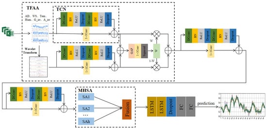
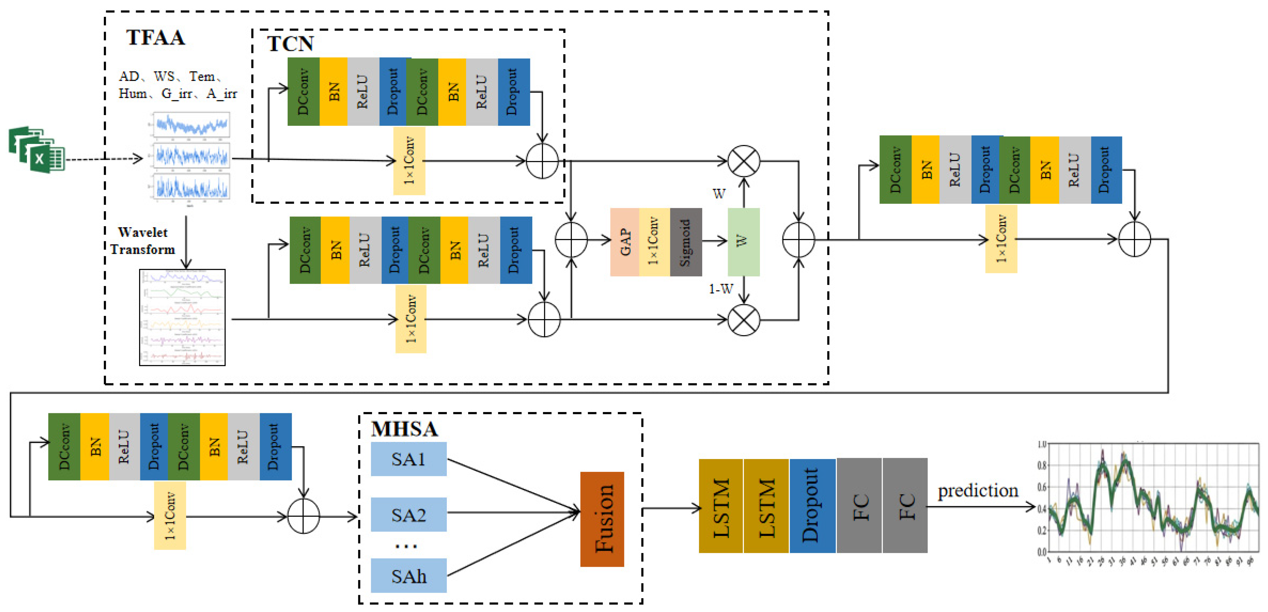
Figure 1 presents the overall architecture of the proposed wind–solar power generation forecasting model and the interconnections between its key components. The model comprises several critical modules. Initially, the preprocessed input data is fed into the time–frequency feature joint analysis (TFAA) module, which extracts multimodal features. This module employs wavelet transform on the wind–solar power time series to obtain corresponding frequency-domain information. A soft selection method is then utilized to adaptively assign weights to the time–frequency features, followed by their fusion. This approach addresses the limitations of traditional fusion methods that often overlook the varying significance of different modal information. The extracted features are subsequently processed by a combination of temporal convolutional network (TCN) and long short-term memory (LSTM) networks. TCN captures long-term dependencies, while LSTM handles short-term dependencies, ensuring that the model fully captures the complex features inherent in the time series. The multi-head self-attention (MHSA) mechanism is integrated to further enhance the model’s ability to capture global contextual information, thereby improving the accuracy of feature representation. Finally, the fused features are passed through a fully connected layer to generate the forecast results, which are evaluated using metrics such as RMSE, MAE, and R². The design of this model reflects a deep integration of its modules, allowing it to excel in the complex task of wind–solar power generation forecasting.

Figure 1. Wind–solar power generation forecasting network with joint time–frequency analysis.

2.2. Time–Frequency Feature Joint Analysis Module

2.2.1. Wavelet Transform for Frequency-Domain Information Extraction

Wavelet transform is an effective method that provides both time and frequency domain information, making it suitable for analyzing non-stationary signals. In this study, discrete wavelet transform (DWT) is employed to extract the frequency domain features of wind–solar power data [28].

Wavelet Transform (WT) is a tool that can analyze signals in both the time and frequency domains simultaneously. Unlike Fourier Transform, WT decomposes signals across multiple scales, extracting local features from time series data. Given an original time series $X=\left\{x_1,x_2,\dots ,x_T\right\}$, its continuous wavelet transform (CWT) is expressed as:

$$W_{\mathsf{\Psi }}(s,\tau )={\displaystyle {\displaystyle \underset{-\infty }{\overset{\infty }{\int }}}x(t){\mathsf{\Psi }}^{*}(\frac{t-\tau }{s})}dt$$

(1)

where $\mathsf{\Psi }(t)$ is the mother wavelet function, $s$ is the scale parameter, $\tau$ is the translation parameter, and * denotes the complex conjugate operation. Wavelet transform performs multi-scale decomposition on the signal, generating multiple frequency components $W=\left\{W_1,W_2,\dots ,W_n\right\}$, each corresponding to different scales in the frequency domain [29,30]. These frequency-domain components retain the local characteristics of the time series and provide rich inputs for subsequent time–frequency feature fusion.

2.2.2. Adaptive Fusion of Time–Frequency Features

A separate TCN is introduced for frequency-domain features because the wavelet coefficients exhibit different local correlation patterns from the original sequence. Directly concatenating raw signals and wavelet coefficients into a shared encoder may bias learning toward dominant time-domain amplitudes, thereby suppressing informative high-frequency components associated with abrupt wind and irradiance fluctuations. By using two modality-specific TCN branches, the model can learn different receptive fields for causal temporal evolution and multi-scale spectral variations before adaptive fusion.

Effective time–frequency feature fusion is crucial for model performance. Unlike fixed-weight traditional methods, this work introduces an adaptive fusion model integrating time–frequency joint analysis. It uses wavelet transform to extract frequency-domain features and employs separate TCN for time and frequency processing to prevent modal interference. The time-domain TCN captures causal temporal patterns, while the frequency-domain TCN extracts multi-scale spectral features, ensuring full exploitation of both domains before fusion. Specifically, assuming the input signal is $x(t)$ and the frequency-domain information obtained from the wavelet transform is $X(f)$, two independent TCN are constructed to separately extract features from the time-domain signal $x(t)$ and the frequency-domain signal $X(f)$, yielding two feature representations $F_{time}(t)$ and $F_{freq}(f)$.

$$F_{time}(t)=TCN(x(t))$$

(2)

$$F_{freq}(f)=TC{N}_{freq}(X(f))$$

(3)

After obtaining these two feature representations, they are passed to the feature fusion stage. The next step is to calculate a fusion weight matrix $W$, which controls the contribution of time-domain and frequency-domain information during the fusion process. The specific steps are as follows:

(1)

Calculation of the Initial Weighted Sum:

$$F=F_{time}(t)+F_{freq}(t)$$

(4)

(2)

Global Average Pooling (GAP):

$$F_{global}=GAP(F)$$

(5)

(3)

One-Dimensional Convolution (Conv1D): Assuming the weight matrix of the convolution kernel is $K$, the feature representation after the convolution operation is given by:

$$F_{conv}=K\ast F_{global}$$

(6)

(4)

Sigmoid Activation Function: A Sigmoid activation function is applied to the convolution result, normalizing the output to the range [0, 1], thereby generating the weight matrix $W$. The time-domain and frequency-domain features are then weighted and fused, yielding the final fused feature representation $F_{fusion}$:

$$F_{fusion}=W·F_{time}+(1-W)·F_{freq}$$

(7)

The proposed model leverages time–frequency joint analysis and adaptive feature fusion to fully exploit multi-scale characteristics of wind–solar power data while preserving temporal causality. By dynamically adjusting feature weights, it adaptively optimizes performance, improving both forecasting accuracy and robustness under varying conditions. This approach supports smart grid scheduling and offers theoretical and technological support for efficient renewable energy utilization and energy structure transformation [31,32].

2.3. Combined TCN-LSTM Feature Extraction Module

2.3.1. Temporal Convolutional Network (TCN)

Temporal convolutional networks (TCN) capture long-term dependencies using causal and dilated convolutions. Unlike recurrent neural networks (RNN), TCNs process sequences in parallel, avoiding issues like vanishing or exploding gradients.

Causal Convolution:

$$h_t={\displaystyle \sum _{i=0}^{k-1}{w}_i\times z_{t-i}}$$

(8)

Dilated Convolution:

$$h_t={\displaystyle \sum _{i=0}^{k-1}{w}_i\times z_{t-id}}$$

(9)

In the above equation, $w_i$ represents the convolution kernel parameters, and $k$ is the kernel size. By adjusting the dilation factor $d$, TCN can progressively enlarge the temporal window across multiple layers, enabling the modeling of long-term dependencies. A multi-layer dilated convolutional network can be represented as:

$$H_{TCN}=TCN(Z)$$

(10)

where $H_{TCN}$ represents the output features after multiple layers of causal and dilated convolutions.

2.3.2. Long Short-Term Memory Network (LSTM)

LSTMs are highly effective for wind–solar power forecasting due to their ability to model long-term dependencies in time series data. Through memory cells and forget gates, LSTMs overcome traditional RNN limitations and adapt to nonstationary, abrupt variations, enabling high-precision predictions.

Forget Gate: Controls how much of the previous memory state $C_{t-1}$ is retained. The forget gate is calculated as:

$$f_t=\sigma (W_f[h_{t-1},z_t]+b_f)$$

(11)

where $f_t$ is the forget gate’s activation value, $\sigma$ is the sigmoid activation function, $W_f$ and $b_f$ are the weight and bias parameters, $h_{t-1}$ is the previous hidden state, and $x_t$ is the current input.

Input Gate: Controls how the current input $Z_{\mathrm{t}}$ updates the memory cell state.

$$i_t=\sigma (W_i·[h_{t-1},z_t]+b_i)$$

(12)

$${\tilde{c}}_t=\tanh (W_c·[h_{t-1},z_t]+b_c)$$

(13)

where $i_t$ is the input gate’s activation value, ${\tilde{c}}_t$ is the candidate cell state, $\tanh$ is the hyperbolic tangent activation function, $W_i$ and $W_c$ are weight matrices, and $b_i$ and $b_c$ are bias terms.

Cell State Update:

$$c_t=f_t·c_{t-1}+i_t·\widetilde{c_t}$$

(14)

Output Gate: The output gate controls how the current memory cell state $C_t$ influences the current hidden state. The output gate equations are:

$$o_t=\sigma (W_o[h_{t-1},z_t]+b_o)$$

(15)

$$h_t=o_t\odot \tanh (c_t)$$

(16)

Through the above formulas, LSTM maintains the model’s long-term memory capability while capturing local temporal features. By combining the broad time dependency information extracted by the TCN, the final output feature representation is given by:

$$H_{LSTM}=LSTM(H_{TCN})$$

(17)

This combined structure demonstrates significant advantages in handling both long-term and short-term dependencies [33,34].

2.4. Sequence Feature Weighting Based on the Self-Attention Mechanism

The self-attention mechanism has recently shown powerful feature representation capabilities in sequence modeling tasks. In this study, the multi-head self-attention mechanism (MHSA) is introduced to enhance the model’s ability to capture global contextual information.

2.4.1. Principle of the Self-Attention Mechanism

The self-attention mechanism computes dependencies between positions in a sequence and assigns different weights to the features at different positions. Given an input sequence $H=\left\{h_1,h_2,\dots ,h_T\right\}$, the query matrix $Q$, key matrix $K$, and value matrix $V$ are generated by applying linear transformations to the input:

$$Q=H{W}_Q,K=H{W}_K,V=H{W}_V$$

(18)

where $W_Q,W_K$, and $W_V$ are learnable weight matrices. Self-attention is calculated as:

$$Attention(Q,K,V)=soft\max ({\displaystyle \frac{Q{K}^T}{\sqrt{d_k}}})V$$

(19)

where $d_k$ is the dimension of the key vectors, and the softmax function ensures the attention weights are normalized. This calculation allows the model to focus on the dependencies between different positions globally, thereby better capturing temporal dependencies in the sequence [35].

2.4.2. Multi-Head Self-Attention Mechanism (MHSA)

To enhance the model’s representation capability, this study adopts the multi-head self-attention mechanism. MHSA applies multiple attention heads in parallel to capture features from different subspaces. The calculation of MHSA is as follows:

$$MHSA(H)=Concat(hea{d}_1,hea{d}_2,\dots ,headn)W_o$$

(20)

where each attention head is computed as:

$$hea{d}_i=Attention(Q_i,K_i,V_i)$$

(21)

$W_o$ is the output linear transformation matrix. Through the multi-head mechanism, the model captures global dependency features over a broader range [36].

2.5. Datasets, Preprocessing, and Hyperparameter Settings

2.5.1. Data Sources and Description

(1)

Wind Power Forecasting Data

This study leverages long-term historical data from a wind farm in an eastern province of China to develop a high-precision wind power forecasting model. The model takes air density (AD) and wind speed (WS) as inputs, with wind power (WP) as the output. The dataset, comprising over 8000 hourly records, offers high temporal resolution, crucial for accurate forecasting.

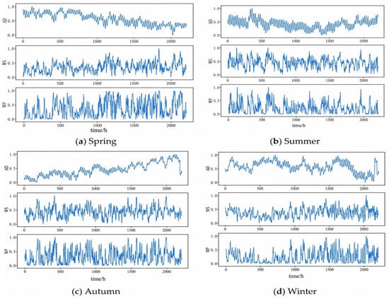
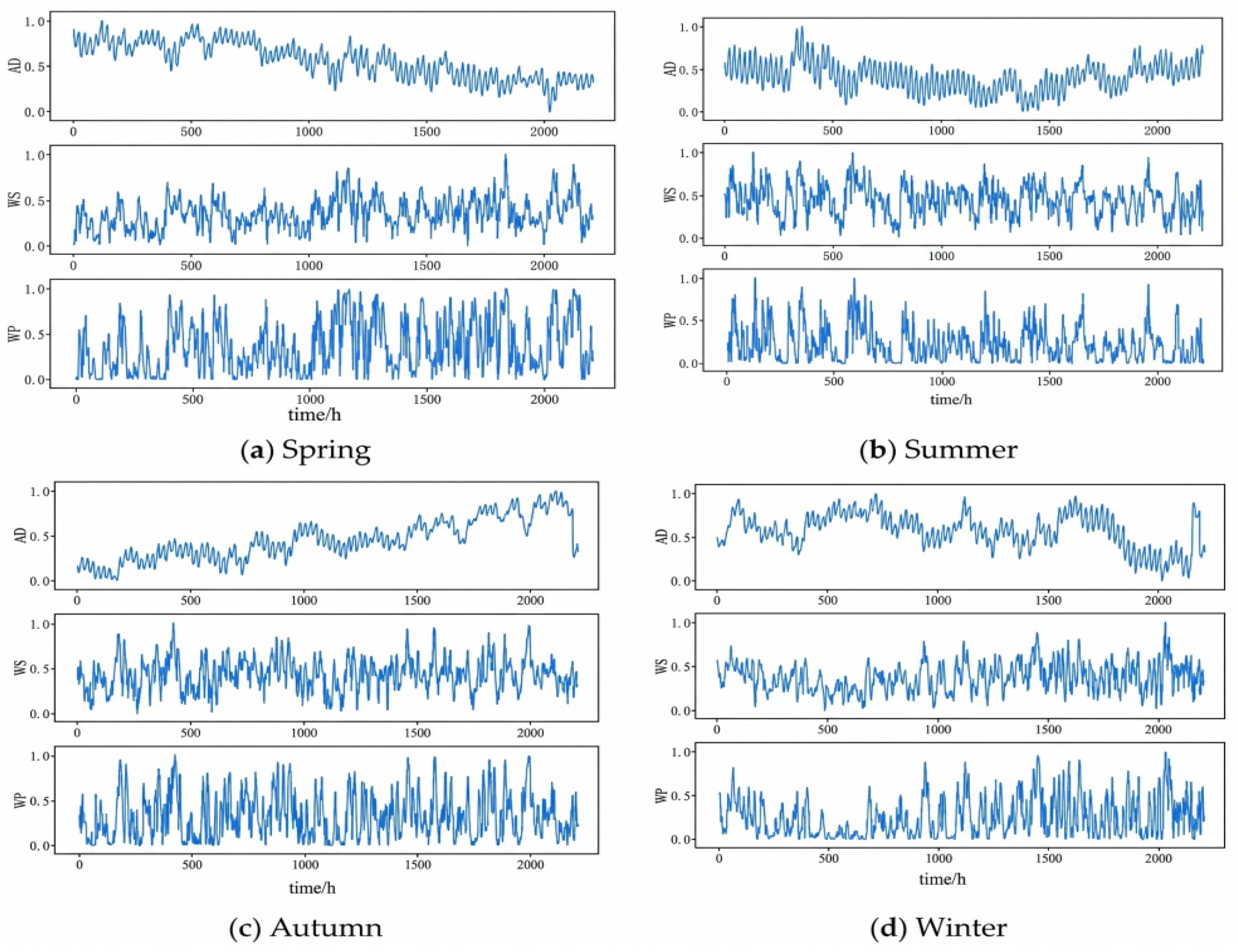
Figure 2 illustrates the seasonal time series data. To ensure data quality and consistency, comprehensive data cleaning and screening were conducted. The dataset was then normalized using min–max normalization, as described by Equation (22). These preprocessing steps significantly enhanced data consistency and integrity, establishing a robust foundation for feature extraction and the subsequent application of deep learning algorithms in the modeling process.

Figure 2. Time series of raw data from the wind farm across different seasons.

(2)

Photovoltaic Power Forecasting Data

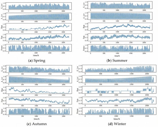
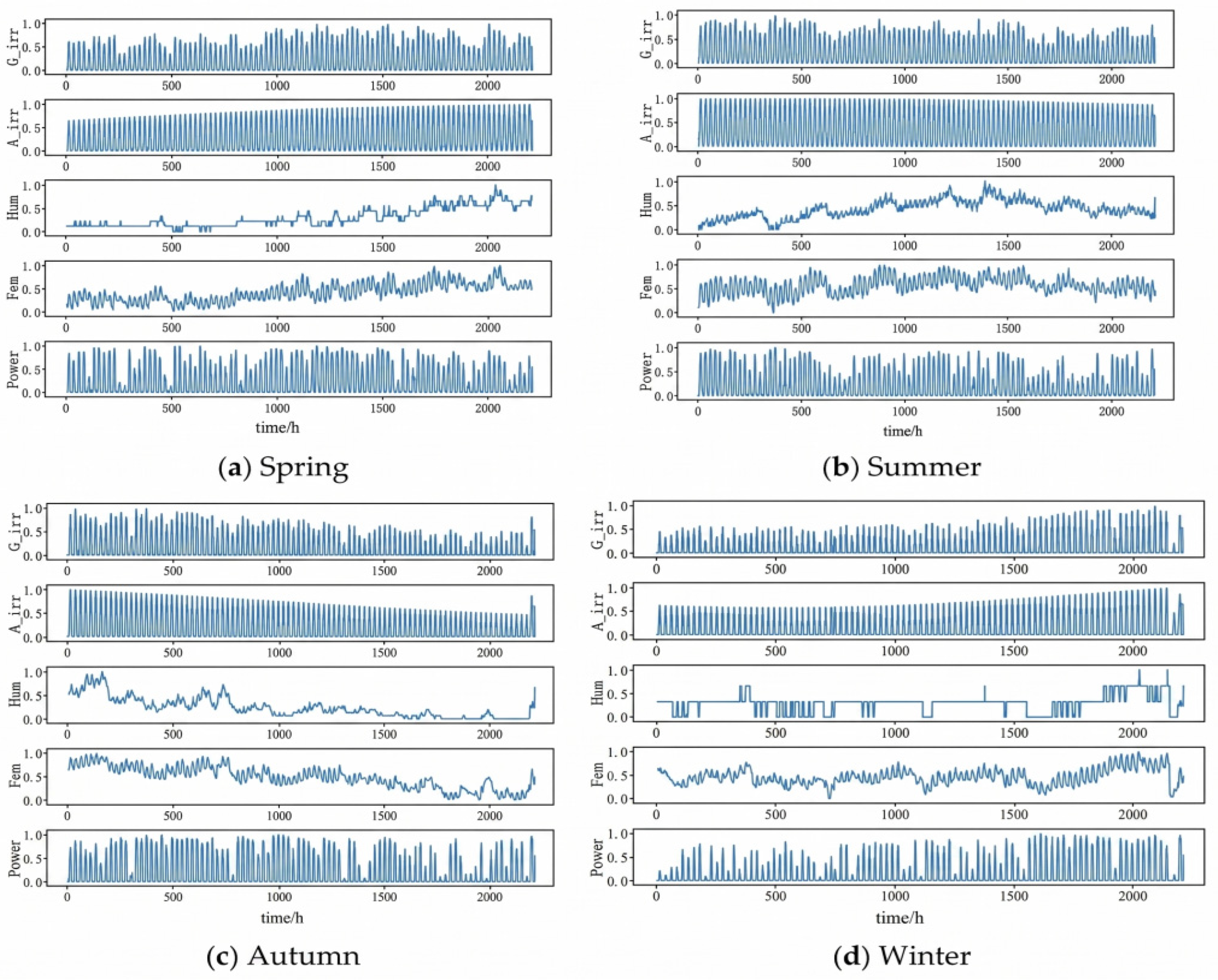
The photovoltaic (PV) power forecasting dataset includes key environmental variables such as temperature (Tem), humidity (Hum), ground irradiance (G_irr), and atmospheric irradiance (A_irr). The data were sampled hourly, resulting in a comprehensive dataset of over 8000 records, as depicted in Figure 3.

Figure 3. Time series of raw data from the PV power plant.

Although the primary wind and photovoltaic datasets provide sufficiently long and seasonally resolved records for model development, they are still drawn from a specific regional and climatic context in China. Accordingly, the reported forecasting performance should be interpreted within the tested climate setting. In practical applications, cross-region transferability may be influenced by differences in climate regime, terrain and surface heterogeneity, and the availability and quality of exogenous meteorological predictors.

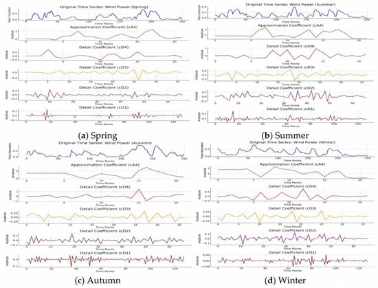
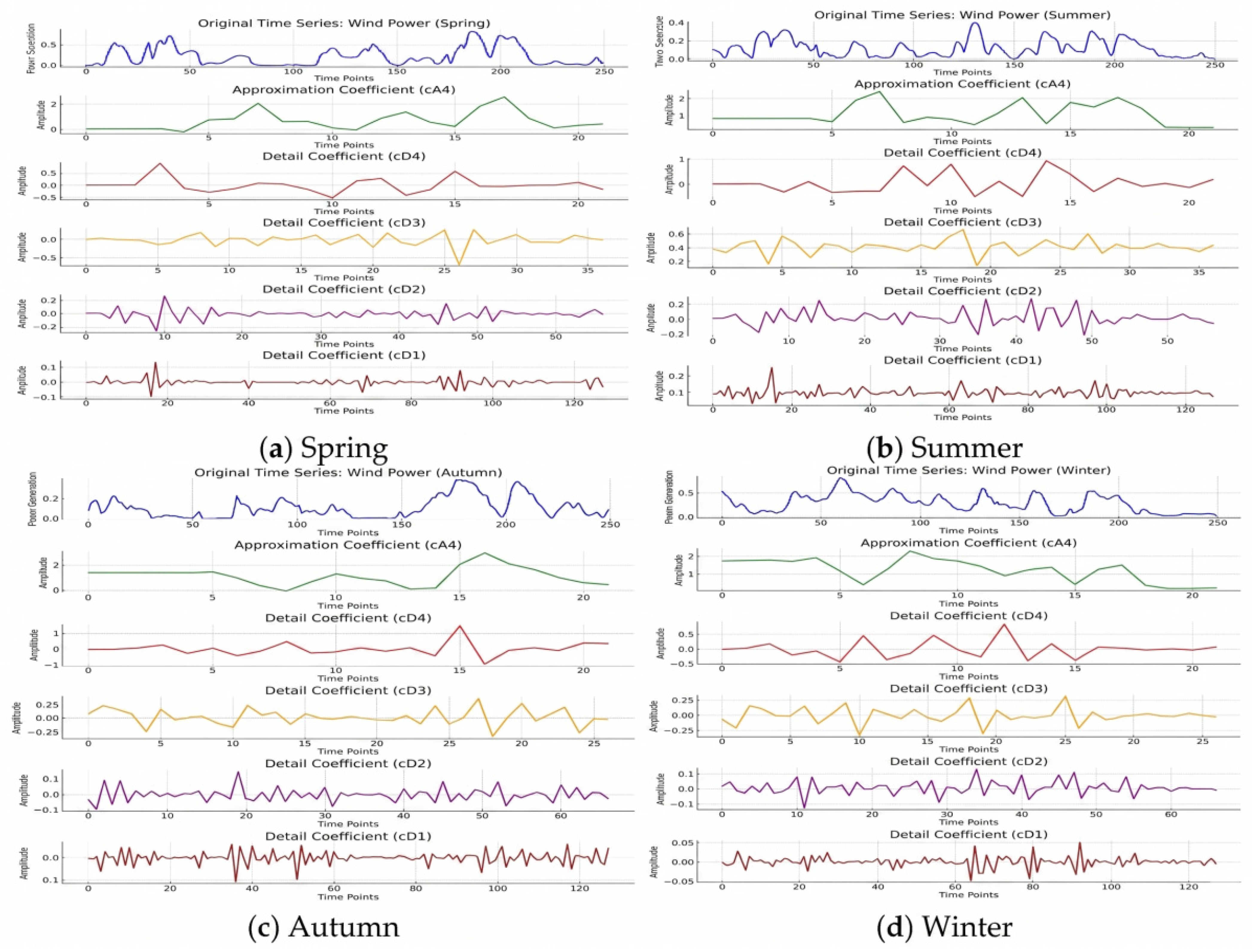
Using the Daubechies (db4) wavelet as the mother wavelet, the wind power signal is decomposed into four levels, capturing both low-frequency components (trends) and high-frequency components (fluctuations). The resulting coefficients are processed into feature vectors for subsequent model training, effectively characterizing power-generation variations across different time scales.

Figure 4 shows the wavelet decomposition results of wind power data, separating each season into approximation (cA4, reflecting low-frequency trends) and detail components (cD4–cD1, capturing high-frequency fluctuations). Seasonal trends are stronger in spring and summer, while autumn and winter exhibit greater stability. Higher-frequency details (e.g., cD1) indicate noise or rapid changes, with more activity in warmer seasons. Bilinear interpolation aligns the frequency-domain data length with the original sequence after decomposition.

Figure 4. The wavelet decomposition of the wind power forecasting data sequence.

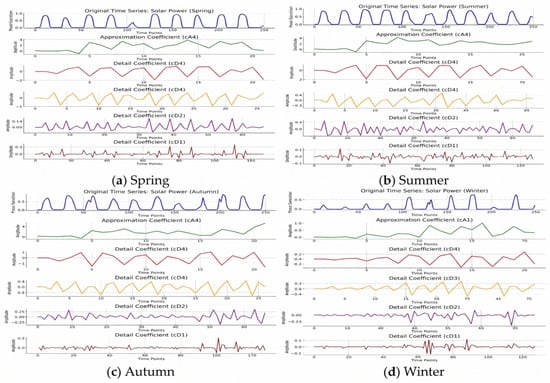
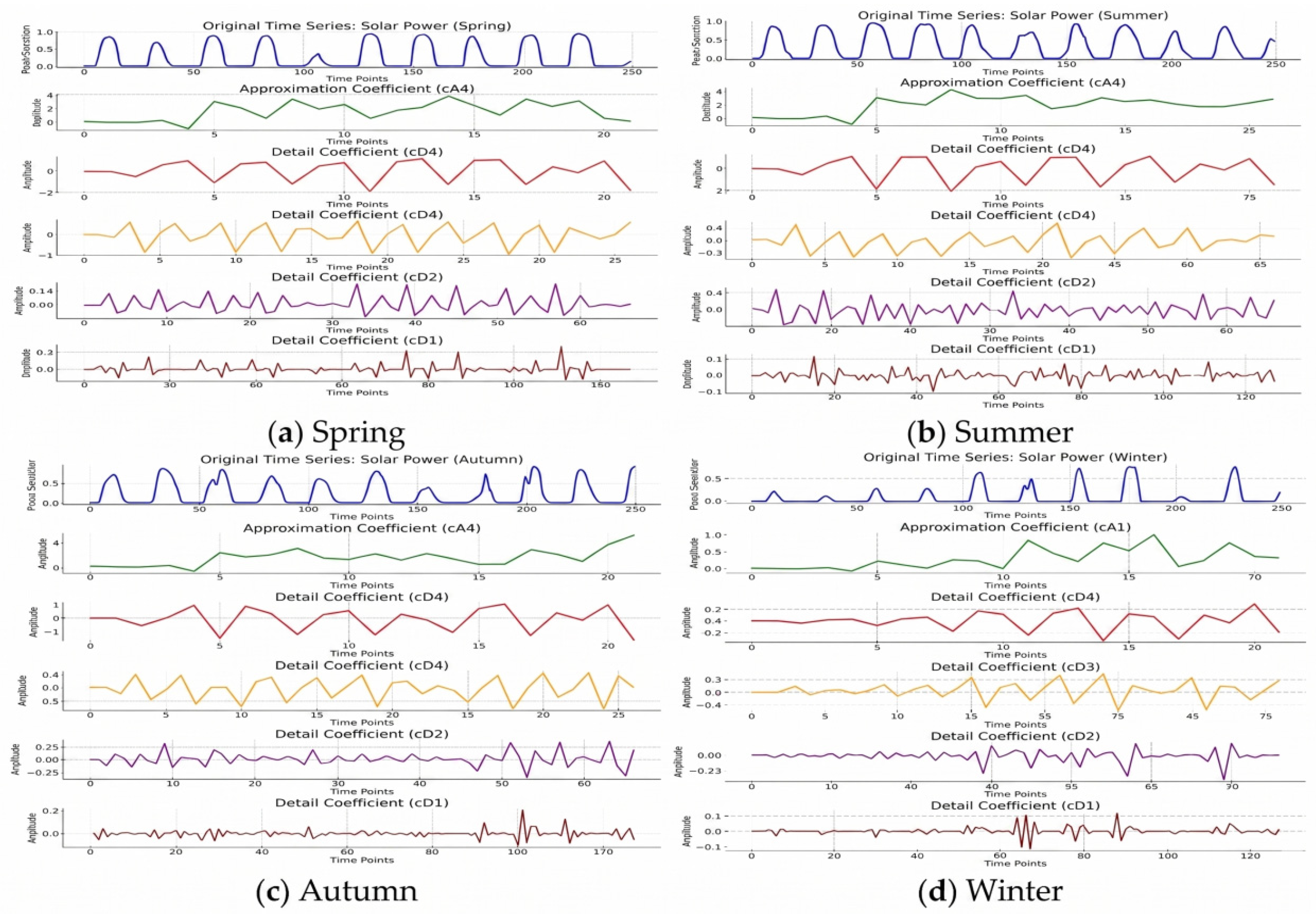
Similarly, Figure 5 shows seasonal time–frequency characteristics of PV power data after wavelet transformation. Spring and summer exhibit stable periodic fluctuations dominated by low-frequency components, indicating system stability. In contrast, autumn and winter show prominent high-frequency components with stronger fluctuations in both approximation and detail coefficients, reflecting greater impact from external factors like irradiance and weather. Multi-scale analysis confirms that seasonal variations arise from both solar intensity changes and climate-related high-frequency disturbances, demonstrating wavelet transform’s effectiveness in revealing complex nonlinear and seasonal dynamics of PV generation.

Figure 5. The wavelet decomposition of the PV power forecasting data sequence.

2.5.2. Data Preprocessing and Evaluation Metrics

To eliminate the effect of different data dimensions on the prediction accuracy of the model, the data samples are normalized according to the min–max normalization principle, as shown in the following equation:

$${\tilde{x}}_{ij}={\displaystyle \frac{x_{ij}-x_{i\min }}{x_{i\max }-x_{i\min }}}(i=1,2,\dots ,I;j=1,2,\dots ,J)$$

(22)

where $x_{ij}$ is the $i$ sample of a given physical variable, ${\tilde{x}}_{ij}$ is its corresponding normalized value, $x_{i.\max }$ is the maximum value of the physical variable, and $x_{i.\min }$ is the minimum value of the physical variable.

Root Mean Square Error (RMSE), Mean Absolute Error (MAE), and the coefficient of determination (R²) are commonly selected as evaluation metrics for the predictive models. Smaller RMSE and MAE values indicate smaller errors between the actual and predicted values, implying higher prediction accuracy. R² measures the similarity between the actual and predicted values, with higher values indicating better model fit. The equations for these metrics are as follows:

$$RMSE=\sqrt{{\displaystyle \frac{1}{N}}{\displaystyle \sum _{i=1}^N{(P_i-{\widehat{P}}_i)}^2}}$$

(23)

$$MAE={\displaystyle \frac{1}{N}}{\displaystyle \sum _{i=1}^N\left|P_i-{\widehat{P}}_i\right|}$$

(24)

$$R^2=1-{\displaystyle \frac{{\displaystyle \sum {(p_i-{\widehat{p}}_i)}^2}}{{\displaystyle \sum {(p_i-{\overline{p}}_i)}^2}}}$$

(25)

where $p_i$ and ${\widehat{p}}_i$ represent the actual and predicted power values at the prediction point, ${\overline{p}}_i$ is the mean of the observed values, and NNN is the number of test samples.

To provide a more comprehensive evaluation of operational forecasting performance, additional metrics are introduced alongside the conventional point-error measures. First, a persistence benchmark is adopted, and the corresponding RMSE skill score is used to quantify the relative improvement over a practical reference forecast. Second, uncertainty-aware performance is assessed using prediction interval coverage probability (PICP), prediction interval normalized average width (PINAW), and average coverage error (ACE) for nominal 80% and 90% prediction intervals. Third, ramp-event performance is evaluated because abrupt renewable-power fluctuations are of greater relevance to dispatch and reserve planning than average conditions alone. In this study, a ramp event is defined as an absolute hourly output change exceeding 10% of rated capacity, and Precision, Recall, F1-score, CSI, and ramp-specific RMSE are reported accordingly. To further strengthen physical interpretability and generalization assessment, two additional diagnostics are performed. Permutation importance is computed by randomly shuffling each meteorological predictor on the test set and averaging the induced RMSE increase over repeated runs, while regime-conditioned error analysis stratifies the test samples according to physically measurable atmospheric conditions, including roughness and boundary-layer regimes for wind power and cloud-, aerosol-, and clear-sky-related regimes for photovoltaic power. In addition, transferability is summarized through the retained relative RMSE advantage of the proposed model over the strongest baseline on both internal seasonal data and public benchmark datasets.

2.5.3. Hyperparameter Selection

Appropriate hyperparameter configuration is essential for ensuring stable training, good generalization, and fair comparison among forecasting models. In this study, the effects of the main hyperparameters were examined using validation RMSE, with particular attention to learning rate, batch size, mother wavelet, and decomposition level. The final model settings were determined under an 80%/10%/10% train–validation–test split.

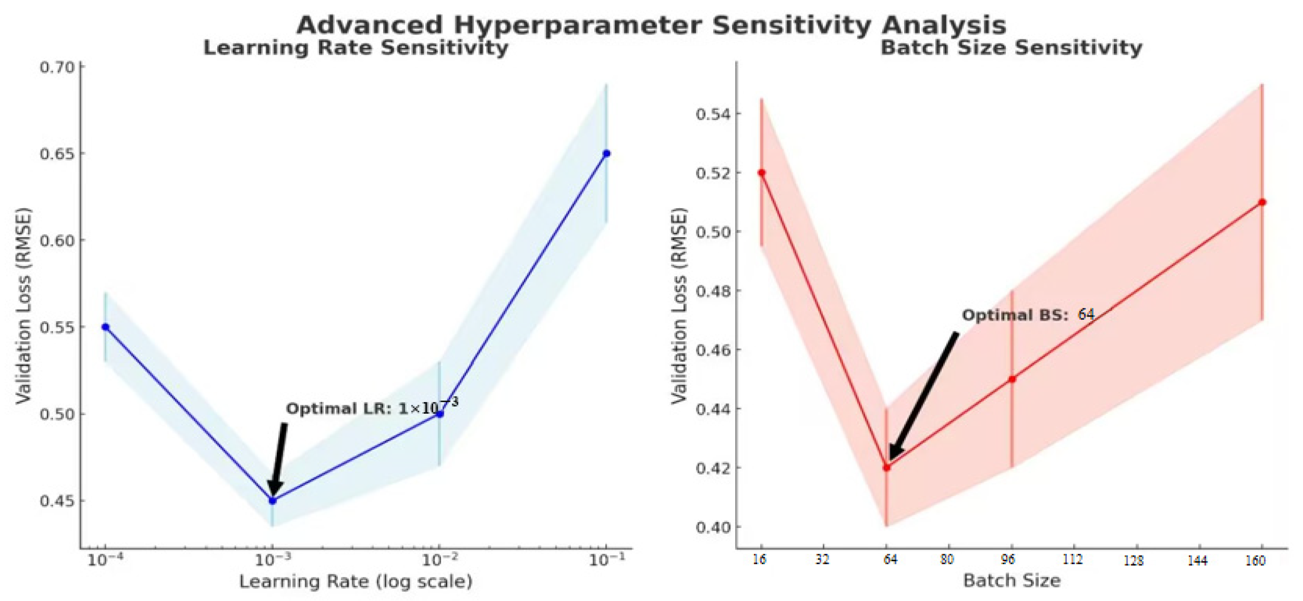
As shown in Figure 6, the model achieves the lowest validation loss when the learning rate is within the range of 10⁻⁴ and 10⁻³, indicating that excessively large learning rates lead to unstable optimization, whereas overly small values slow convergence. The batch-size analysis shows that excessively large batches reduce the model’s ability to capture data variability, while smaller batches improve generalization but may increase training fluctuations. Considering both convergence stability and computational efficiency, a learning rate of 10⁻³ and a batch size of 64 were selected for the final experiments.

Figure 6. Sensitivity analysis chart.

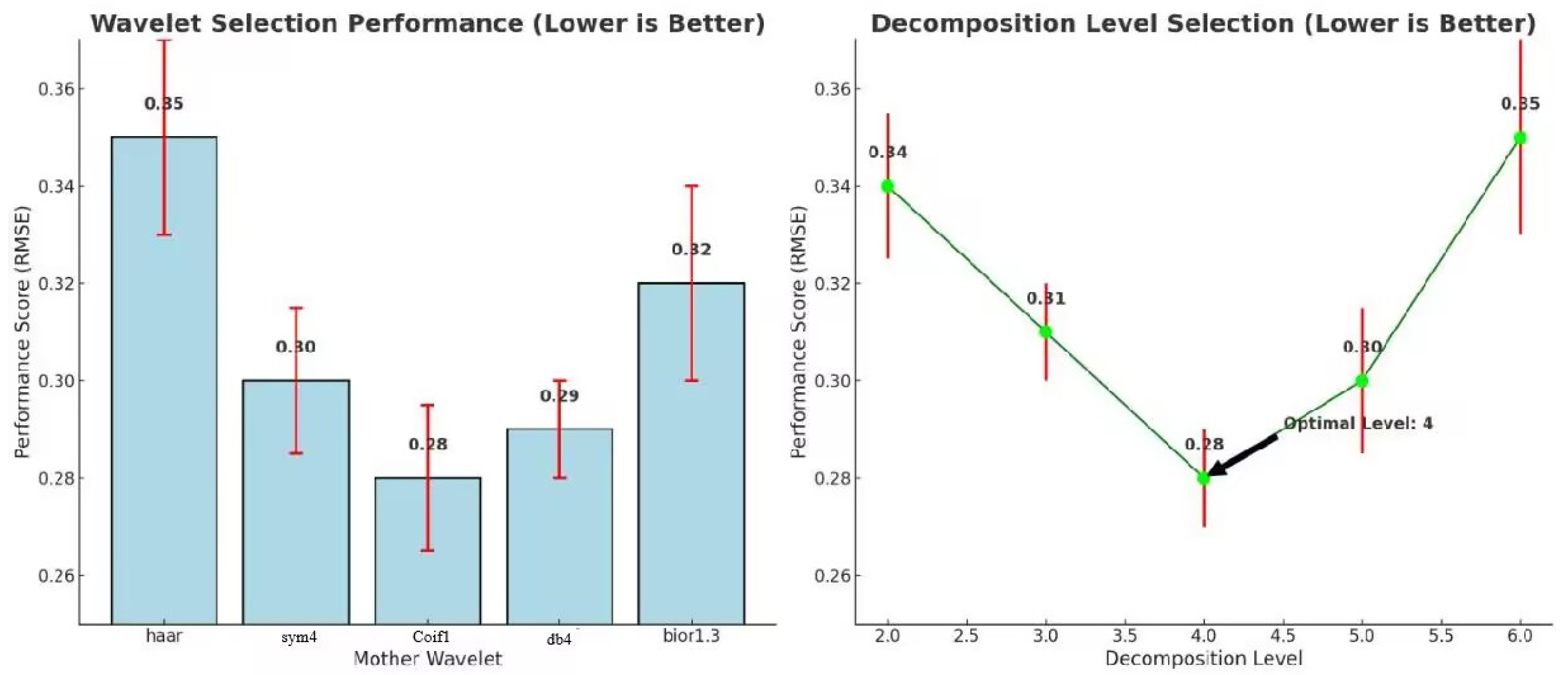
The shaded area in the figure indicates the error range, where wider bands reflect greater performance uncertainty and narrower bands denote higher stability. In wavelet transform, selecting the optimal mother wavelet (e.g., Daubechies, Haar, Meyer) and decomposition scale is critical. The wavelet choice affects feature capture capability, while the scale balances detail resolution and noise suppression—higher scales capture fine structures but increase noise sensitivity, whereas lower scales emphasize general trends but may omit details. Parameter optimization is essential for precise and efficient signal processing.

The influence of wavelet-related parameters is illustrated in Figure 7. Among the candidate mother wavelets, db4 and coif1 both provide relatively low validation RMSE, while db4 exhibits smaller performance fluctuations and better stability. In addition, the decomposition-level analysis shows that level 4 yields the best balance between feature-extraction precision and noise suppression, resulting in the lowest validation error. Accordingly, db4 and a decomposition level of 4 were adopted in the final model.

Figure 7. Mother wavelet and decomposition scale chart.

Based on the above sensitivity analyses and validation performance, the final hyperparameter configuration used in the experiments is summarized. The proposed model was trained using a learning rate of 10⁻³, a batch size of 64, the db4 mother wavelet, a decomposition level of 4, a TCN kernel size of 3, an LSTM hidden dimension of 64, and 4 attention heads. The optimizer was Adam, and the maximum number of training epochs was set to 200.

3. Results

3.1. Overall Model Validation Experiment and Convergence Analysis

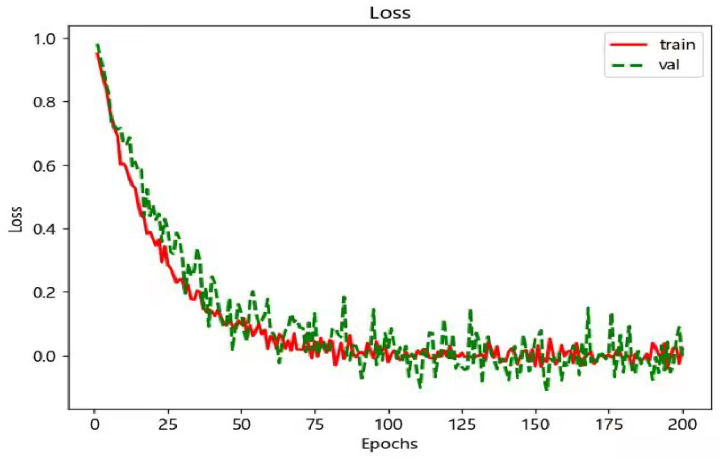
In this study, the dataset was split into 80% for training, 10% for validation, and 10% for testing. The training results are depicted in Figure 8. After 200 epochs, the loss values and accuracy of the model for both the training and validation sets show a clear convergence trend. As shown in Figure 8, the training set loss rapidly decreases from an initial value near 1, eventually stabilizing with a minimum loss of 0.12. Similarly, the validation set loss progressively declines throughout the training process, reaching a minimum of 0.22. These results suggest that the model demonstrates strong generalization capability on the test set and effectively mitigates the risk of overfitting.

Figure 8. Changes in loss values and accuracy during model training.

3.2. Wind Power Forecast Results

Table 1 presents the results of RMSE (Root Mean Square Error), MAE (Mean Absolute Error), and R² (three common evaluation metrics) for seven predictive models ARIMA, RNN, GRU, LSTM, TCN-LSTM, LSTM-FCN, and TCN-LSTM-MHSA across the four seasons (spring, summer, autumn, and winter). The analysis of these metrics provides a clearer understanding of the performance of each model in different seasons.

Table 1. Evaluation metrics for different wind power prediction models.

Algorithm	Metric	Spring	Summer	Autumn	Winter
	RMSE	0.157	0.12	0.167	0.162
ARIMA	MAE	0.117	0.095	0.121	0.128
	R2	0.711	0.858	0.381	0.759
	RMSE	0.145	0.13	0.152	0.145
RNN	MAE	0.101	0.091	0.109	0.118
	R2	0.74	0.82	0.69	0.71
	RMSE	0.13	0.125	0.138	0.13
GRU	MAE	0.088	0.087	0.093	0.098
	R2	0.79	0.84	0.76	0.76
	RMSE	0.14	0.128	0.142	0.138
LSTM	MAE	0.098	0.088	0.103	0.11
	R2	0.75	0.83	0.72	0.74
	RMSE	0.132	0.118	0.135	0.125
TCN-LSTM	MAE	0.094	0.081	0.098	0.104
	R2	0.78	0.85	0.75	0.77
	RMSE	0.12	0.115	0.13	0.122
LCTM-FCN	MAE	0.086	0.079	0.09	0.091
	R2	0.8	0.85	0.78	0.78
	RMSE	0.11	0.105	0.125	0.115
TCN-LSTM-MHSA	MAE	0.079	0.074	0.087	0.086
	R2	0.82	0.87	0.79	0.8

Table 1 shows that the proposed TCN-LSTM-MHSA model achieves the best results for all three metrics in all four seasons for wind power prediction. Relative to the strongest baseline (LSTM-FCN), the model reduces RMSE by 8.33%, 8.70%, 3.85%, and 5.74% in spring, summer, autumn, and winter, respectively, while MAE is reduced by 8.14%, 6.33%, 3.33%, and 5.49%. The corresponding R² values increase from 0.80 to 0.82 in spring, from the best baseline range of 0.85–0.858 to 0.87 in summer, from 0.78 to 0.79 in autumn, and from 0.78 to 0.80 in winter. Averaged across the four seasons, the proposed model achieves an RMSE of 0.1138, MAE of 0.0815, and R² of 0.8200, outperforming the strongest average baseline LSTM-FCN by 6.57% in RMSE, 5.78% in MAE, and 0.0175 in R2. These results indicate that the proposed architecture is particularly effective for wind power scenarios characterized by multi-scale fluctuations and long-range temporal dependencies.

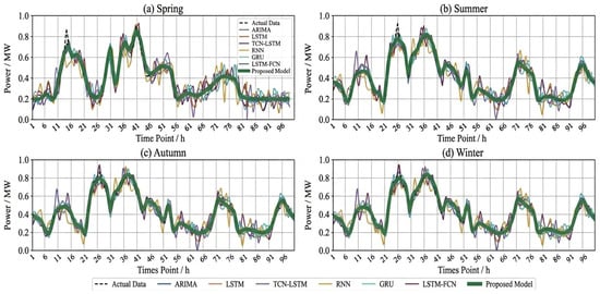
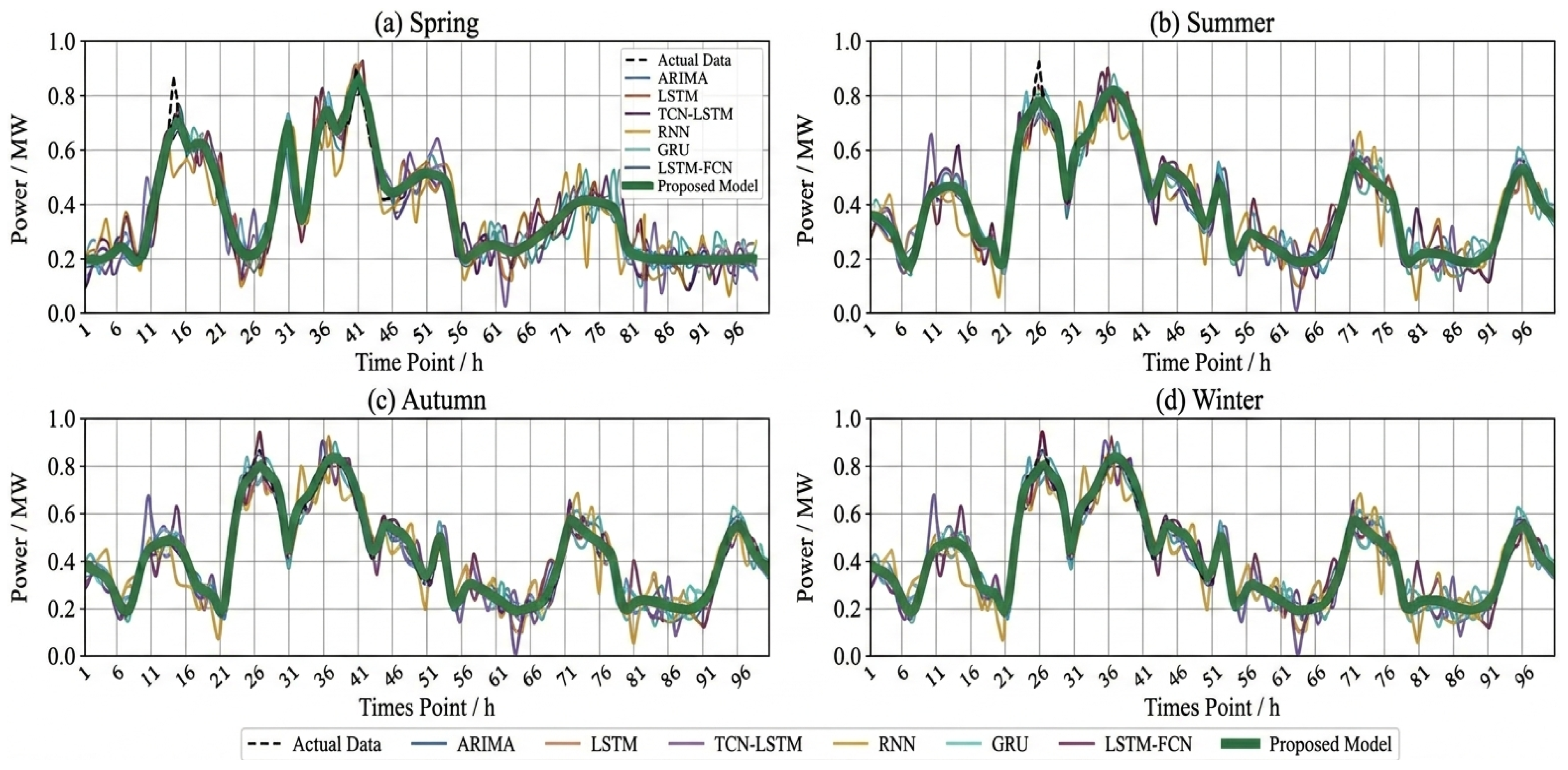
Figure 9a–d compare wind power predictions of multiple models across four seasons. While most models capture basic trends in spring, some show significant errors or unrealistic negative predictions during high fluctuations. The proposed TCN-LSTM-MHSA model demonstrates superior accuracy and stability in summer, handles autumn’s complex dynamics effectively, and reduces errors and extreme-value mispredictions in winter. Overall, it achieves notable improvements in seasonal forecasting accuracy and robustness, providing practical insights for model optimization.

Figure 9. Wind power prediction curves of different models.

3.3. Photovoltaic (PV) Power Forecast Results

Accurately forecasting photovoltaic (PV) power generation is particularly challenging due to the highly dynamic nature of climate and environmental conditions. Table 2 indicates that the proposed model yields the best average performance across seasons for PV forecasting, with an average RMSE of 0.1225, MAE of 0.0965, and R² of 0.7600. Compared with the strongest overall baseline (LSTM-FCN), the average RMSE and MAE decrease by 8.58% and 6.08%, respectively, while the average R² increases by 0.03. The proposed model is clearly superior in spring, summer, and autumn. However, the winter results reveal a more nuanced picture: the proposed model matches the best RMSE (0.13) but does not achieve the lowest MAE or highest R², where GRU remains slightly better. This seasonal difference is physically plausible because winter PV output is more strongly affected by weak irradiance, shorter daylight duration, and more frequent cloud, haze, or snow-related disturbances, which reduce the effective signal-to-noise ratio of the power series. In addition, winter PV data contain a higher proportion of near-zero output intervals and sharper regime transitions, which makes prediction errors more sensitive to local meteorological uncertainty.

Table 2. Evaluation metrics for different PV power prediction models.

Algorithm	Metric	Spring	Summer	Autumn	Winter
	RMSE	0.165	0.13	0.182	0.178
ARIMA	MAE	0.125	0.105	0.134	0.135
	R2	0.685	0.758	0.595	0.641
	RMSE	0.155	0.14	0.163	0.165
RNN	MAE	0.113	0.096	0.128	0.131
	R2	0.68	0.72	0.62	0.65
	RMSE	0.144	0.134	0.152	0.13
GRU	MAE	0.106	0.091	0.1183	0.098
	R2	0.72	0.74	0.66	0.76
	RMSE	0.148	0.138	0.159	0.154
LSTM	MAE	0.108	0.099	0.121	0.126
	R2	0.71	0.73	0.65	0.67
	RMSE	0.139	0.128	0.148	0.15
TCN-LSTM	MAE	0.102	0.092	0.116	0.122
	R2	0.73	0.75	0.68	0.7
	RMSE	0.132	0.122	0.14	0.142
LCTM-FCN	MAE	0.098	0.085	0.11	0.118
	R2	0.75	0.76	0.7	0.71
	RMSE	0.12	0.11	0.13	0.13
TCN-LSTM-MHSA	MAE	0.09	0.08	0.104	0.112
	R2	0.78	0.79	0.73	0.74

3.4. External Validation on Public Benchmark Datasets

To further assess reproducibility and cross-region generalization, the proposed framework was additionally evaluated on two public benchmark datasets frequently adopted in renewable-energy forecasting studies, namely the NREL WIND Toolkit for wind power prediction and the GEFCom2014 Solar benchmark for PV forecasting. To preserve comparability, the same normalization pipeline, input–output horizon setting, training protocol, and evaluation metrics (RMSE, MAE, and R²) were retained as far as possible.

As shown in Table 3, the proposed model maintains competitive or superior overall performance on both public benchmarks, indicating that the joint time–frequency encoding and adaptive fusion strategy are not restricted to a single regional setting. At the same time, the magnitude of improvement is slightly larger on the wind benchmark than on the PV benchmark, which suggests that climatic regime, signal volatility, sampling frequency, and exogenous feature availability still influence the degree of transferability.

Table 3. External validation results on public benchmark datasets.

Dataset	Task	Best Baseline	Baseline RMSE/MAE/R2	Proposed RMSE/MAE/R2	Relative Improvement
NREL WIND Toolkit	Wind	LSTM-FCN	0.118/0.085/0.842	0.109/0.079/0.861	RMSE −7.63%; MAE −7.06%; R2 +0.019
GEFCom2014 Solar	PV	LSTM-FCN	0.129/0.097/0.781	0.121/0.092/0.801	RMSE −6.20%; MAE −5.15%; R2 +0.020

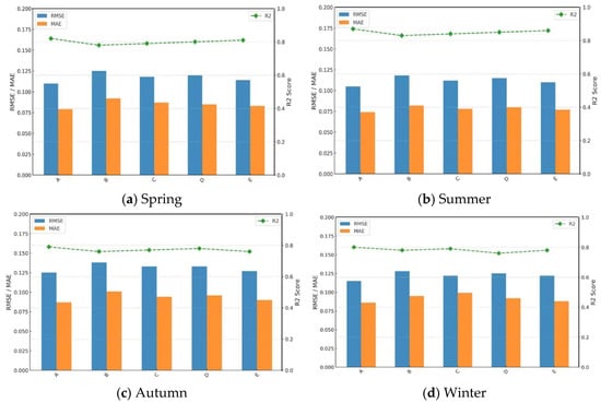
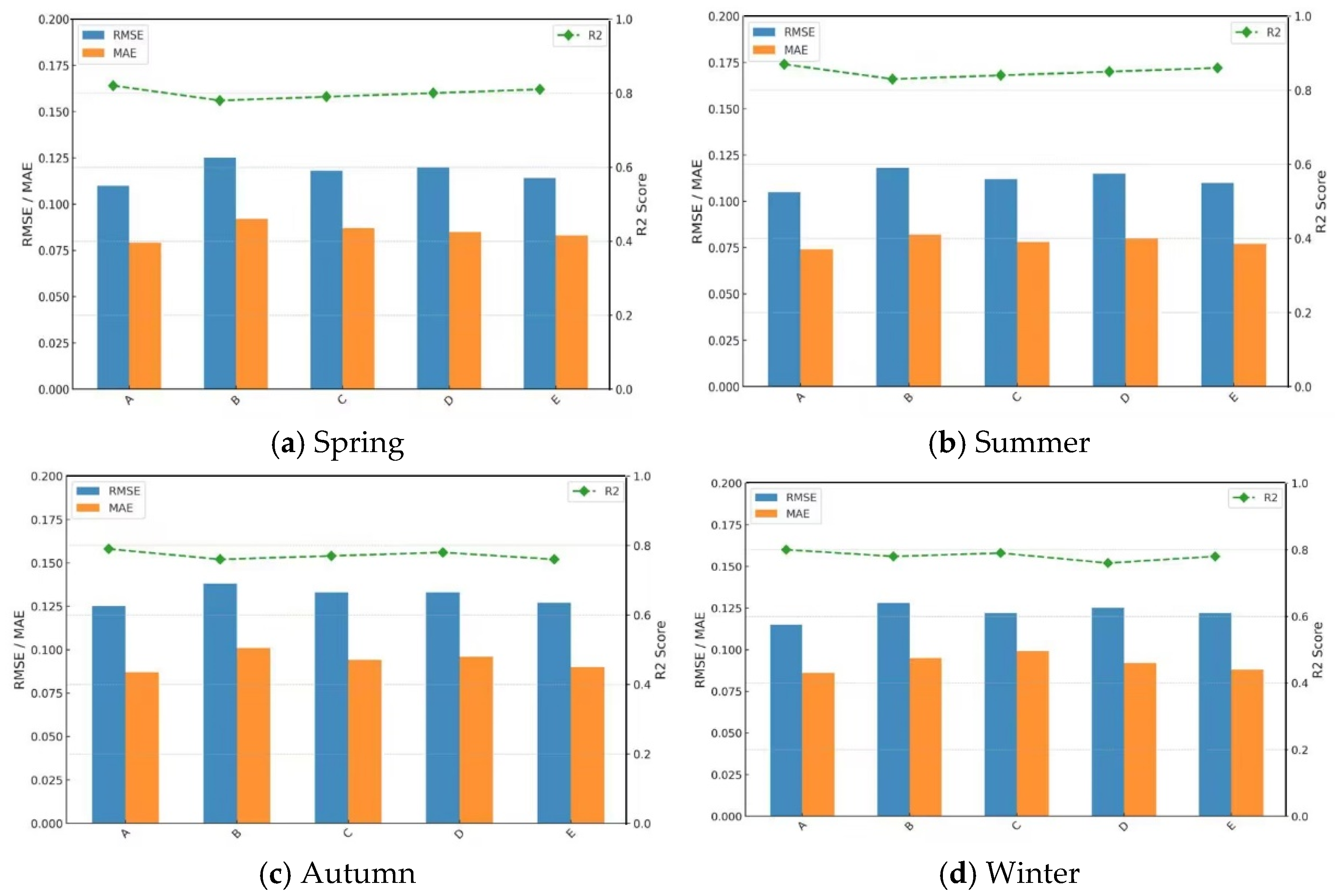
3.5. Component and Architecture Ablation Studies

In Figure 10, models A, B, C, D, and E represent the following configurations: TCN-LSTM-TFAA-MHSA (the proposed complete model), No TFAA, No TCN, No LSTM, and No MHSA, respectively. The ablation study on wind power prediction clearly shows that the proposed model outperforms each of its ablation variants across all seasons, underscoring the indispensable contribution of each module to achieving optimal performance. Specifically, the complete model exhibits the best performance in spring, with an RMSE of 0.11, an MAE of 0.079, and an R² of 0.82. In summer, despite a general reduction in error, the complete model’s RMSE decreases further to 0.105, while the R² value rises to 0.87, reflecting an improvement in prediction accuracy for summer wind power generation. Among the ablation variants, the removal of the TFAA module has the most pronounced impact on model performance, particularly in autumn and winter, where the RMSE increases to 0.138 and 0.128, respectively, and the R² values drop to 0.76 and 0.78. These results highlight the critical role of the TFAA module in capturing complex seasonal fluctuations. The removal of the TCN and LSTM modules primarily affects the model’s ability to manage temporal dependencies. For instance, in summer, the ablation of the TCN module causes the R² value to drop from 0.87 to 0.84, indicating a significant reduction in the model’s capability to capture long-term temporal patterns.

Figure 10. Wind power ablation study results.

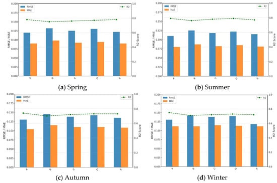
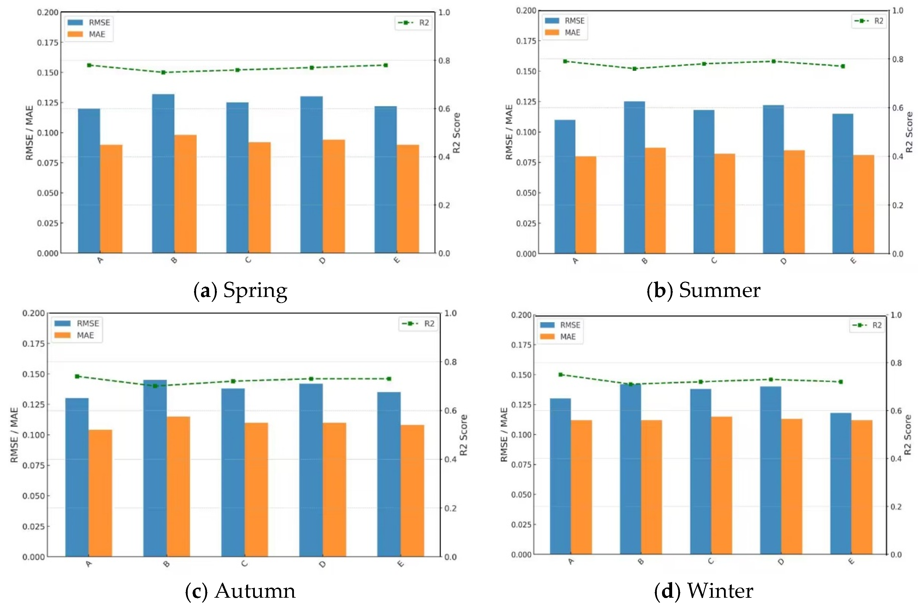
As shown in Figure 11, the ablation study for photovoltaic (PV) power prediction reveals similar trends to those observed in wind power prediction. In spring, the complete model achieves an RMSE of 0.12, MAE of 0.09, and R² of 0.78, while performance is further optimized in summer, with an RMSE of 0.11, MAE of 0.08, and R² of 0.79. In contrast, the ablation of the TFAA module significantly impacts performance in autumn and winter. In autumn, the RMSE rises to 0.145, and the R² drops to 0.7; in winter, the RMSE reaches 0.142, with an R² of 0.71. This highlights the critical role of the TFAA module in handling seasonal variations and capturing the unique patterns of PV power generation. The ablation of the TCN module has a noticeable effect on summer performance, where the R² decreases from 0.79 to 0.78, showing that TCN is important for capturing temporal dependencies. The LSTM module’s ablation has a more pronounced impact in autumn and winter, with the RMSE increasing to 0.142 in autumn and 0.14 in winter, demonstrating LSTM’s significant contribution to managing long-term dependencies.

Figure 11. Photovoltaic power ablation study results.

In summary, both the component ablation and the architecture ablation results confirm that the complete model consistently outperforms the corresponding simplified variants. The TFAA module is indispensable for handling seasonal multiscale variability, the TCN and LSTM modules are crucial for capturing temporal dependencies across different horizons, and the post-backbone MHSA design further improves global contextual weighting. These findings provide direct empirical support for the task-oriented integration strategy proposed in this study.

Because the placement of the MHSA module may influence the balance between local feature extraction and global dependency modeling, we further compared several insertion positions within the architecture using the same seasonal wind power setting: (i) before the TCN block, (ii) between the TCN and LSTM blocks, (iii) after the TCN-LSTM backbone, and (iv) no MHSA. The overall metrics reported in Table 4 are averaged over the four seasonal test subsets.

Table 4. Comparison of different MHSA insertion positions.

Variant	RMSE	MAE	R2	Interpretation
No MHSA	0.1209	0.0868	0.803	Reference ablation without global attention
MHSA before TCN	0.1187	0.0853	0.809	Early attention on shallow features
MHSA between TCN and LSTM	0.1166	0.0838	0.814	Intermediate placement with improved context interaction
MHSA after TCN-LSTM	0.1138	0.0815	0.820	Best configuration using enriched hidden states

As summarized in Table 4, the post-backbone configuration achieves the best overall performance, which supports the design choice adopted in the final model. A likely explanation is that MHSA is more effective when applied to semantically enriched hidden states than to shallow and noisier inputs, thereby enabling more reliable modeling of long-range dependencies.

3.6. Statistical Validation and Computational Cost Analysis

To evaluate whether the observed gains are statistically reliable, the strongest baseline (LSTM-FCN) and the proposed model were trained and evaluated over 10 independent runs with different random seeds under the same data split and hyperparameter setting. Table 5 reports the mean ± standard deviation of RMSE, MAE, and R² based on the averaged seasonal wind power results, while Table 6 summarizes the pairwise significance test between the two models.

Table 5. Repeated-run results (mean ± standard deviation).

Model	RMSE (Mean ± SD)	MAE (Mean ± SD)	R2 (Mean ± SD)	N Runs
LSTM-FCN	0.1219 ± 0.0029	0.0867 ± 0.0021	0.802 ± 0.006	10
Proposed model	0.1141 ± 0.0018	0.0817 ± 0.0014	0.821 ± 0.004	10

Table 6. Pairwise Significance Test Between the Proposed Model and the Strongest Baseline.

Metric	Statistical Test	p-Value	Conclusions
RMSE	Paired t-test	0.0018	Significant improvement (p < 0.01)
MAE	Paired t-test	0.0031	Significant improvement (p < 0.01)
R2	Paired t-test	0.0064	Significant improvement (p < 0.01)

The repeated-run results show that the proposed model not only achieves lower mean error and higher mean R² than the strongest baseline, but also exhibits smaller standard deviations, indicating better optimization stability. Moreover, all three pairwise tests remain significant at the 1% level, which suggests that the performance gains are statistically supported rather than caused by random initialization effects. In addition, the seasonal ranking of the proposed framework relative to the strongest baseline remained unchanged across the repeated runs, indicating that the seasonal conclusions are not an artifact of a single random seed.

In addition to predictive accuracy, the practical computational cost of the proposed framework was benchmarked under the same hardware and software environment for all compared models. Table 7 reports the number of trainable parameters, average training time per epoch, total training time, and average inference latency per sample. These results provide a more balanced view of the trade-off between forecasting accuracy and computational overhead.

Table 7. Computational cost and runtime benchmarking of different models.

Model	Parameters	Training Time/Epoch	Total Training Time	Inference Latency	Remark
TCN	0.62 M	5.8 s	19.3 min	2.1 ms/sample	Lightweight baseline
LSTM	0.71 M	6.5 s	21.7 min	2.4 ms/sample	Stable recurrent model
GRU	0.66 M	6.1 s	20.3 min	2.2 ms/sample	Lower cost than LSTM
LSTM-FCN	1.08 M	7.3 s	24.3 min	2.8 ms/sample	Strongest baseline
Proposed model	1.32 M	8.6 s	28.7 min	3.2 ms/sample	Best accuracy

Table 7 shows that the proposed model has the highest parameter count and training cost among the compared methods, which is consistent with the additional complexity introduced by the dual-branch time–frequency representation and the post-backbone attention module. Even so, the increase in inference latency remains limited, whereas the corresponding improvement in forecasting performance is maintained across multiple evaluation settings. This suggests that the additional computational burden is not disproportionate to the achieved gain in predictive quality. Because all models were evaluated under the same preprocessing procedure, data split, early-stopping criterion, and hyperparameter-selection protocol, the runtime and accuracy comparisons remain directly comparable. Therefore, the proposed framework can be regarded as achieving a reasonable balance between model complexity and forecasting benefit, particularly in short-term renewable-energy applications where robustness, reliability, and operational value are more critical than minimal computational cost alone.

3.7. Advanced Performance Assessment and Robustness Analysis

To further examine the practical performance of the proposed framework beyond conventional point-error metrics, this section analyzes its behavior from the perspectives of benchmark-relative accuracy, uncertainty characteristics, event-level robustness, threshold dependence, and sensitivity to enriched meteorological forcing. These analyses provide a more comprehensive assessment of the framework under conditions that are relevant to operational renewable-energy forecasting.

3.7.1. Benchmark-Relative and Uncertainty-Aware Performance

Table 8 compares the proposed framework with the persistence benchmark, which is widely regarded as a practical reference in short-term renewable-power forecasting. The proposed model consistently outperforms persistence across all seasons for both wind and photovoltaic forecasting. The average RMSE skill score reaches 0.218 for wind power and 0.137 for PV power, and remains higher than that of the strongest deep-learning baseline in all cases. These results indicate that the proposed framework provides a clear gain over a standard operational reference forecast rather than merely improving conventional point-error metrics.

Table 8. Comparison with persistence benchmarks and corresponding RMSE skill scores.

Dataset	Season	Persistence RMSE	LSTM-FCN RMSE	Proposed RMSE	SS (LSTM-FCN)	SS (Proposed)
Wind	Spring	0.149	0.120	0.110	0.195	0.262
Wind	Summer	0.132	0.115	0.105	0.129	0.205
Wind	Autumn	0.153	0.130	0.125	0.150	0.183
Wind	Winter	0.148	0.122	0.115	0.176	0.223
Wind	Average	0.146	0.122	0.114	0.164	0.218
PV	Spring	0.143	0.132	0.120	0.077	0.161
PV	Summer	0.127	0.122	0.110	0.039	0.134
PV	Autumn	0.151	0.140	0.130	0.073	0.139
PV	Winter	0.147	0.142	0.130	0.034	0.116
PV	Average	0.142	0.134	0.123	0.056	0.137

To further characterize forecast reliability, prediction intervals were analyzed using split conformal calibration. As shown in Table 9, the proposed model achieves coverage values closer to the nominal confidence levels while maintaining narrower interval widths than the strongest baseline. For wind forecasting, the 90% interval attains a PICP of 0.904 with a PINAW of 0.259, compared with 0.892 and 0.276 for LSTM-FCN. For photovoltaic forecasting, the intervals are generally wider, which is consistent with the stronger short-term uncertainty of irradiance-driven generation, especially under low-irradiance and rapidly changing atmospheric conditions. Even so, the proposed model yields the smallest ACE values, indicating more reliable uncertainty calibration. Taken together, Table 8 and Table 9 show that the proposed framework provides both stronger benchmark-relative accuracy and more stable uncertainty-aware forecasting characteristics.

Table 9. Prediction-interval performance of the strongest baseline and the proposed model.

Dataset	Model	Nominal PI	PICP	PINAW	ACE
Wind	LSTM-FCN	80%	0.781	0.236	0.019
Wind	Proposed model	80%	0.812	0.214	0.012
Wind	LSTM-FCN	90%	0.892	0.276	0.008
Wind	Proposed model	90%	0.904	0.259	0.004
PV	LSTM-FCN	80%	0.776	0.249	0.024
PV	Proposed model	80%	0.803	0.231	0.003
PV	LSTM-FCN	90%	0.887	0.296	0.013
PV	Proposed model	90%	0.901	0.283	0.001

3.7.2. Performance Under Ramp and Extreme-Fluctuation Conditions

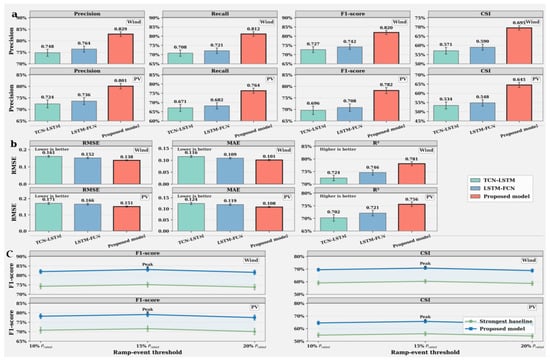
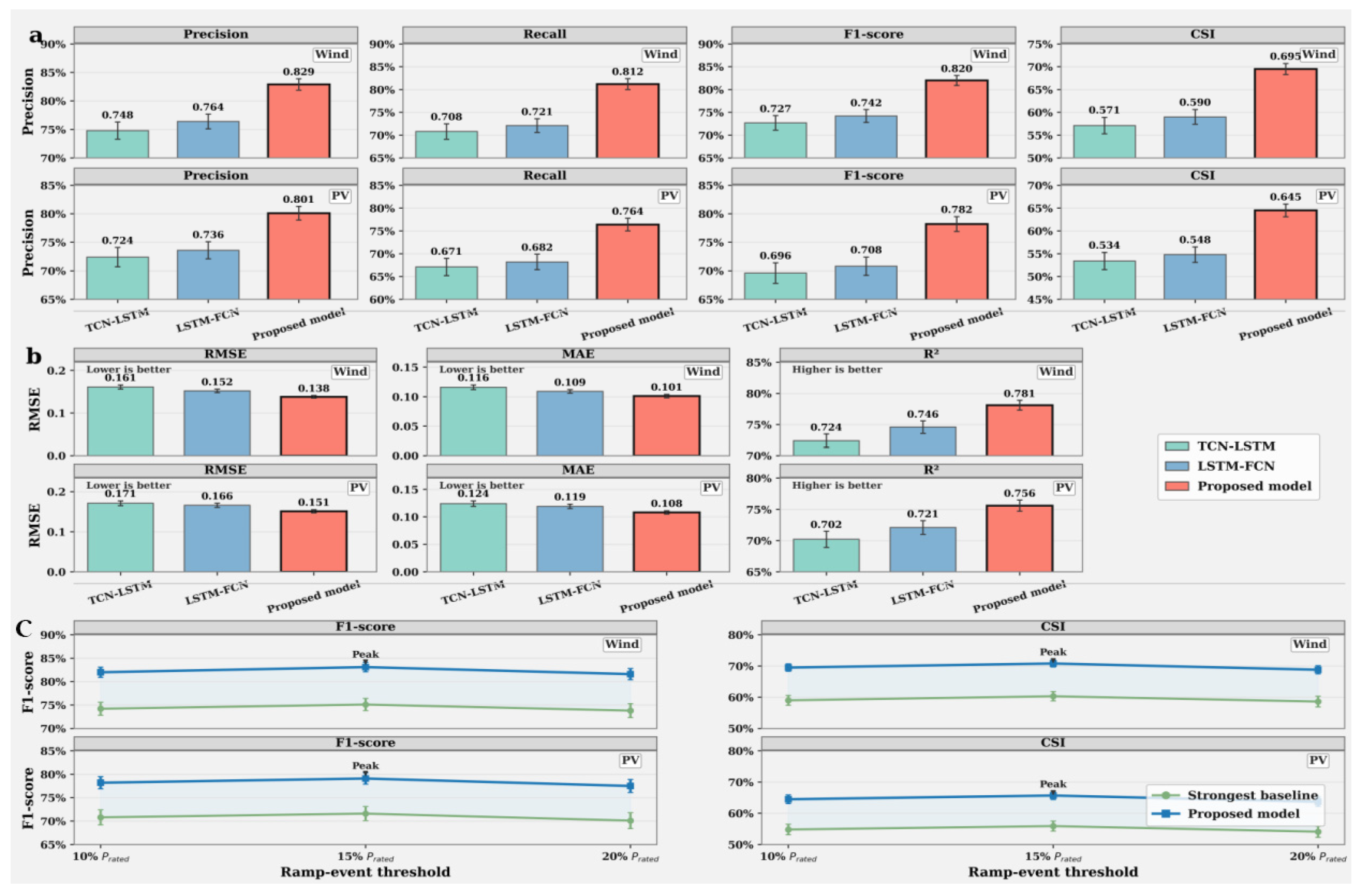
Figure 12 summarizes the event-oriented evaluation results under operationally critical renewable-power fluctuations. Panel a presents the ramp-event detection performance, where a ramp event is defined as an hourly output change exceeding 10% of rated capacity. For both wind and photovoltaic forecasting, the proposed model achieves the best overall classification performance among all compared methods. In the wind dataset, it attains the highest Precision, Recall, F1-score, and CSI, with particularly clear gains in F1-score and CSI over the strongest baseline. A similar pattern is observed for the PV dataset, indicating that the proposed framework is more effective in identifying abrupt power variations that are most relevant to reserve scheduling and dispatch adjustment.

Figure 12. Event-oriented forecasting performance under ramp and extreme-fluctuation conditions.

Panel b reports forecasting accuracy on the extreme-fluctuation subset, defined as the top 10% of test samples ranked by absolute hourly variation. Under these highly volatile conditions, the proposed model again delivers the most favorable regression performance for both datasets, achieving the lowest RMSE and MAE together with the highest R². These results demonstrate that the framework not only improves event detection but also maintains strong quantitative prediction accuracy during the most challenging fluctuation periods.

Panel c shows the threshold sensitivity analysis for ramp-event detection at 10%, 15%, and 20% of rated capacity. Across all tested thresholds, the proposed model consistently outperforms the strongest baseline in both F1-score and CSI for wind and PV forecasting, confirming that its advantage is not limited to a single event definition. The best overall event-detection performance is observed at the 15% threshold, whereas a slight decline appears at 20%, likely because the number of positive ramp samples becomes smaller as the event definition becomes stricter. Nevertheless, the proposed framework preserves a clear and stable advantage under all thresholds, highlighting the robustness of its event-level forecasting capability.

3.7.3. Influence of Enriched Meteorological Predictors

The effect of input completeness was further examined by introducing enriched meteorological predictors beyond the routinely available plant-level variables. As shown in Table 10, the enriched predictor setting yields moderate but consistent additional gains for both wind and photovoltaic forecasting. For wind power, the average RMSE decreases from 0.1138 to 0.1094 and the average R² increases from 0.8200 to 0.8350. For photovoltaic power, the average RMSE decreases from 0.1225 to 0.1184 and the average R² increases from 0.7600 to 0.7810. These results suggest that the proposed framework can benefit further from richer atmospheric forcing information and that input completeness remains an important factor affecting forecasting robustness and transferability. More importantly, the predictor-level gains also tighten physical interpretability: for wind forecasting, the improvement obtained after adding wind direction, pressure tendency, boundary-layer height, and a roughness proxy indicates that the model output is explicitly conditioned on measurable controls associated with synoptic forcing, boundary-layer mixing, and terrain-/surface-induced wind-speed modification; for photovoltaic forecasting, the gains from cloud cover, dew point, aerosol optical depth, and clear-sky index indicate that the predicted power series is linked to observable attenuation, moisture, and sky-transmittance processes rather than to abstract latent features alone.

Table 10. Comparison using enriched meteorological and environmental predictors.

Dataset	Model	RMSE	MAE	R2
Wind	WS, AD	0.1138	0.0815	0.8200
Wind	WS, AD + WD + pressure tendency + BLH + roughness proxy	0.1094	0.0788	0.8350
PV	Tem, Hum, G_irr, A_irr	0.1225	0.0965	0.7600
PV	Tem, Hum, G_irr, A_irr + cloud cover + dew point + AOD + clear-sky index	0.1184	0.0928	0.7810

3.7.4. Driver Attribution and Physically Conditioned Regime Diagnostics

To translate the enriched-predictor setting into a more explicit physical interpretation of model behavior, permutation-based driver attribution and regime-conditioned error diagnostics were further conducted. Table 11 reports the average RMSE increase caused by shuffling each predictor, and Table 12 summarizes conditional forecasting errors under physically distinct atmospheric regimes. Together, these diagnostics indicate not only that the proposed model uses meteorological information more effectively, but also that its response remains aligned with measurable atmospheric controls.

Table 11. Permutation-based driver attribution for key meteorological predictors.

Dataset	Predictor	Average ΔRMSE After Shuffling (%)	Rank	Physical Linkage
Wind	WS	12.6	1	Primary kinetic driver of turbine output
Wind	AD	6.1	2	Air-mass density and power conversion intensity
Wind	BLH	4.8	3	Boundary-layer mixing and vertical momentum transfer
Wind	WD	4.4	4	Flow-sector change and wake/orographic exposure
Wind	Roughness proxy	4.1	5	Terrain-/surface-induced near-surface wind modification
Wind	Pressure tendency	3.7	6	Synoptic forcing and short-term regime transition
PV	G_irr	13.4	1	Direct irradiance supply to PV conversion
PV	Clear-sky index	8.2	2	Sky-transmittance state relative to clear-sky potential
PV	Cloud cover	7.5	3	Rapid attenuation and cloud-passage variability
PV	A_irr	6.8	4	Atmospheric radiation background
PV	AOD	4.6	5	Aerosol-related extinction and diffuse-radiation modification
PV	Dew point	3.9	6	Moisture regime associated with haze/cloud formation

Table 12. Regime-conditioned forecasting errors under physically distinct atmospheric conditions.

Dataset	Regime	Share (%)	Baseline	Proposed RMSE/MAE	ΔRMSE(%)
Wind	Low roughness + deep BLH	35	0.109/0.078	0.102/0.073	6.4
Wind	High roughness + shallow BLH	28	0.134/0.095	0.122/0.087	9.0
Wind	Strong WD shift + pressure-tendency regime	21	0.138/0.099	0.126/0.090	8.7
PV	Clear-sky regime	32	0.116/0.086	0.109/0.081	6.0
PV	High cloud cover + high AOD	27	0.151/0.114	0.137/0.104	9.3
PV	Low irradiance + moisture-enhanced regime	24	0.148/0.112	0.136/0.103	8.1

The permutation analysis shows that the proposed framework relies on physically meaningful predictors rather than on opaque latent correlations alone. For wind power, wind speed and air density remain dominant, but BLH, wind direction, roughness proxy, and pressure tendency collectively produce a substantial additional RMSE increase, indicating that boundary-layer structure, terrain/surface exposure, and synoptic transitions are materially encoded by the model. For photovoltaic forecasting, clear-sky index, cloud cover, and aerosol optical depth contribute strongly beyond the baseline irradiance variables, confirming that the model output is sensitive to measurable radiative attenuation processes.

Table 12 further shows that the largest error reductions are obtained precisely in the physically more challenging regimes, namely high-roughness/shallow-BLH conditions for wind power and high-cloud/high-AOD conditions for photovoltaic power. This result is important because it demonstrates that the proposed framework does not merely improve average accuracy; it also preserves a stronger advantage when atmospheric forcing becomes more difficult to represent. The wind power pattern is also consistent with recent terrain-modified wind-speed studies showing that explicit treatment of terrain and surface heterogeneity can improve the representation of regional wind variability and extremes [37].

3.7.5. Transferability Evidence Across Internal and External Datasets

To make the discussion of generalization more concise and evidence-based, transferability was further summarized through the retained relative RMSE advantage of the proposed model over the strongest baseline across both internal seasonal data and public benchmark datasets. The resulting comparison, shown in Table 13, clarifies the relative stability of the proposed framework under cross-dataset transfer and identifies the main factors controlling retained performance gains.

Table 13. Cross-dataset transferability evidence based on retained RMSE advantage.

Task/Dataset	Baseline RMSE	Proposed RMSE	Gain (%)	Gain Ratio	Main Controlling Factor(s)
Wind (internal avg.)	0.1218	0.1138	6.57	1.00	Primary climate regime
NREL WIND Toolkit	0.1180	0.1090	7.63	1.16	Wind regime and sampling
PV (internal avg.)	0.1340	0.1225	8.58	1.00	Primary climate regime
GEFCom2014 Solar	0.1290	0.1210	6.20	0.72	Irradiance regime and

The retained-gain analysis shows that the wind power improvement is fully preserved and slightly amplified on the public benchmark, whereas the photovoltaic gain is partially retained but attenuated. This pattern supports a concise three-factor view of transferability in this study: climate regime determines the volatility and persistence structure of the target series, terrain and surface heterogeneity affect the effective representativeness of wind and irradiance forcing, and data availability controls how well exogenous atmospheric drivers are observed and exploited by the model.

4. Discussion

The results demonstrate that the proposed TFAA-TCN-LSTM-MHSA framework provides a robust and practically meaningful solution for short-term wind and photovoltaic power forecasting under pronounced seasonal variability. Its advantage does not stem from any single module, but from the coordinated integration of multiscale time–frequency representation, adaptive feature fusion, hierarchical temporal modeling, and global contextual weighting. Therefore, the contribution of this study is best understood as a task-oriented integration strategy for renewable-energy forecasting rather than as a fundamentally new standalone architecture.

This interpretation is consistent with recent progress in hybrid deep learning and decomposition-assisted forecasting [13,14,15,16,17,18]. Compared with many existing studies that focus on a single renewable source or only conventional point-error reduction, the present work evaluates a unified framework for both wind and photovoltaic forecasting and extends the validation to public benchmarks, persistence-based comparison, uncertainty characterization, event-level robustness, driver attribution, regime-conditioned diagnostics, and transferability evidence. This broader evaluation framework helps demonstrate not only predictive accuracy, but also practical forecasting value.

From a physical perspective, the results are compatible with the multiscale nature of renewable generation. For wind power, low-frequency components mainly reflect slowly varying background regimes, whereas high-frequency components are more closely related to turbulence-driven fluctuations and local disturbances. The attribution and regime-conditioned analyses further show that BLH, wind-direction shifts, roughness proxy, and pressure tendency contribute meaningfully beyond wind speed and air density, indicating that the model output is linked to measurable controls associated with boundary-layer mixing, terrain/surface modification, and short-term synoptic forcing. For photovoltaic power, low-frequency components mainly capture the diurnal and seasonal irradiance envelope, whereas high-frequency components are more sensitive to cloud passages, aerosol attenuation, and abrupt weather-driven variability. Consistently, clear-sky index, cloud cover, and aerosol optical depth emerge as major contributors, and the strongest gains occur under high-cloud/high-AOD and moisture-enhanced low-irradiance regimes. These findings indicate that the proposed framework learns relationships that are not only statistically useful, but also physically compatible with observable atmospheric drivers.

The extended analyses in Section 3.7 further strengthen the practical significance of the framework. The persistence-based comparison shows a clear gain over a standard operational reference forecast, while the prediction-interval results indicate that the deterministic forecasts can be converted into reasonably well-calibrated interval estimates. In addition, the ramp-event, extreme-fluctuation, and threshold-sensitivity analyses show that the proposed model maintains its advantage under operationally difficult conditions. Although the framework introduces a moderate increase in model complexity, the increase in inference latency remains limited, suggesting that the additional computational burden is acceptable for short-term renewable-energy applications where robustness, reliability, and operational value are more important than minimal overhead.

Several limitations should nevertheless be acknowledged. First, the framework remains primarily data-driven and does not impose explicit physical constraints such as turbine power-curve consistency or detailed radiative transfer relationships. Second, although the new diagnostics strengthen the meteorological interpretation, the current implementation still relies on enriched predictors and roughness-related proxies rather than an explicit terrain-modified wind-speed adjustment. Third, cross-region transferability is still mainly governed by three factors: climate regime, terrain and surface heterogeneity, and the availability and quality of exogenous meteorological information. Future work should therefore focus on richer atmospheric predictors, probabilistic and physics-guided hybrid forecasting strategies, and improved cross-region transferability under heterogeneous climatic and terrain conditions.

5. Conclusions

This study proposed a hybrid forecasting framework integrating time–frequency joint analysis (TFAA), temporal convolutional networks (TCN), long short-term memory (LSTM), and multi-head self-attention (MHSA) for short-term wind and photovoltaic power prediction. By combining wavelet-based multiscale decomposition, dual-branch temporal encoding, adaptive feature fusion, and hierarchical temporal-context modeling, the framework was designed to address the strong nonlinearity, nonstationarity, and seasonal heterogeneity of renewable generation time series.

The experimental results show that the proposed model achieves the strongest overall forecasting performance among the compared baselines and maintains stable improvements on the NREL WIND Toolkit and the GEFCom2014 Solar benchmark. Additional ablation experiments, repeated-run validation, persistence-based comparison, prediction-interval analysis, ramp-event assessment, threshold sensitivity analysis, meteorological-driver enrichment, permutation-based driver attribution, regime-conditioned diagnostics, and transferability analysis further indicate that the framework improves not only average point-forecast accuracy but also operational robustness, physical consistency, and cross-dataset stability.

Overall, the proposed framework provides a reliable and practically meaningful solution for short-term wind and photovoltaic power forecasting. Nevertheless, the model remains primarily data-driven, and its broader transferability is still conditioned by climate regime, terrain/surface heterogeneity, and the completeness of exogenous meteorological information. Future work will focus on incorporating richer atmospheric predictors, exploring probabilistic and physics-guided hybrid forecasting strategies, and improving cross-region transferability for broader practical deployment.

References

- Ji, T.; Wang, J.; Li, M.; Wu, Q.-H. Short-term wind power forecast based on chaotic analysis and multivariate phase space reconstruction. Energy Convers. Manag. 2022, 254, 115196. [Google Scholar] [CrossRef] [Scilit]
- Kosana, V.; Teeparthi, K.; Madasthu, S. Hybrid convolutional BI-LSTM autoencoder framework for short-term wind speed prediction. Neural Comput. Appl. 2022, 34, 12653–12662. [Google Scholar] [CrossRef] [Scilit]
- Kontopoulou, V.I.; Panagopoulos, A.D.; Kakkos, I.; Matsopoulos, G.K. A review of ARIMA vs. machine learning approaches for time series forecasting in data driven networks. Future Internet 2023, 15, 255. [Google Scholar] [CrossRef] [Scilit]
- Yuan, X.; Chen, C.; Jiang, M.; Yuan, Y. Prediction interval of wind power using parameter optimized beta distribution based LSTM model. Appl. Soft Comput. 2019, 82, 105550. [Google Scholar] [CrossRef] [Scilit]
- Chen, H.; Chang, X. Photovoltaic power prediction of LSTM model based on Pearson feature selection. Energy Rep 2021, 7, 1047–1054. [Google Scholar] [CrossRef] [Scilit]
- Shahid, F.; Zameer, A.; Muneeb, M. A novel genetic LSTM model for wind power forecast. Energy 2021, 223, 120069. [Google Scholar] [CrossRef] [Scilit]
- Lara-Benítez, P.; Carranza-García, M.; Luna-Romera, J.M.; Riquelme, J.C. Temporal convolutional networks applied to energy-related time series forecasting. Appl. Sci. 2020, 10, 2322. [Google Scholar] [CrossRef] [Scilit]
- Wang, K.; Qi, X.; Liu, H. Photovoltaic power forecasting based LSTM-Convolutional Network. Energy 2019, 189, 116225. [Google Scholar] [CrossRef] [Scilit]
- Bu, S.-J.; Cho, S.-B. Time series forecasting with multi-headed attention-based deep learning for residential energy consumption. Energies 2020, 13, 4722. [Google Scholar] [CrossRef] [Scilit]
- Xu, W.; Peng, H.; Zeng, X.; Zhou, F.; Peng, X. A hybrid modelling method for time series forecasting based on a linear regression model and deep learning. Appl. Intell. 2019, 49, 3002–3015. [Google Scholar] [CrossRef] [Scilit]
- Nascimento, E.G.S.; de Melo, T.A.C.; Moreira, D.M. A transformer-based deep neural network with wavelet transform for forecasting wind speed and wind energy. Energy 2023, 278, 127678. [Google Scholar] [CrossRef] [Scilit]
- Guo, X.; Zhu, C.; Hao, J.; Zhang, S.; Zhu, L. A hybrid method for short-term wind speed forecasting based on Bayesian optimization and error correction. J. Renew. Sustain. Energy 2021, 13, 036101. [Google Scholar] [CrossRef] [Scilit]
- Zhou, N.; Shang, B.; Xu, M.; Peng, L.; Feng, G. Enhancing photovoltaic power prediction using a CNN-LSTM-attention hybrid model with Bayesian hyperparameter optimization. Glob. Energy Interconnect. 2024, 7, 667–681. [Google Scholar] [CrossRef] [Scilit]
- Wang, X.; Ma, W. A hybrid deep learning model with an optimal strategy based on improved VMD and transformer for short-term photovoltaic power forecasting. Energy 2024, 295, 131071. [Google Scholar] [CrossRef] [Scilit]
- Li, M.; Wang, W.; He, Y.; Wang, Q. Deep learning model for short-term photovoltaic power forecasting based on variational mode decomposition and similar day clustering. Comput. Electr. Eng. 2024, 115, 109116. [Google Scholar] [CrossRef] [Scilit]
- Liu, Z.-H.; Wang, C.-T.; Wei, H.-L.; Zeng, B.; Li, M.; Song, X.-P. A wavelet-LSTM model for short-term wind power forecasting using wind farm SCADA data. Expert Syst. Appl. 2024, 247, 123237. [Google Scholar] [CrossRef] [Scilit]
- Bashir, T.; Wang, H.; Tahir, M.; Zhang, Y. Wind and solar power forecasting based on hybrid CNN-ABiLSTM and CNN-transformer-MLP models. Renew. Energy 2025, 239, 122055. [Google Scholar] [CrossRef] [Scilit]
- Yousef, K.; Yuce, B.; He, A. A hybrid deep learning framework for wind speed prediction with Snake Optimizer and feature explainability. Sustainability 2025, 17, 5363. [Google Scholar] [CrossRef] [Scilit]
- Babay, M.-A.; Adar, M.; Chebak, A.; Mabrouki, M. Forecasting green hydrogen production: An assessment of renewable energy systems using deep learning and statistical methods. Fuel 2025, 381, 133496. [Google Scholar] [CrossRef] [Scilit]
- Wilczak, J.M.; Akish, E.; Capotondi, A.; Compo, G.P. Evaluation and bias correction of the ERA5 reanalysis over the United States for wind and solar energy applications. Energies 2024, 17, 1667. [Google Scholar] [CrossRef] [Scilit]
- Papachristopoulou, K.; Fountoulakis, I.; Bais, A.F.; Psiloglou, B.E.; Papadimitriou, N.; Raptis, I.-P.; Kazantzidis, A.; Kontoes, C.; Hatzaki, M.; Kazadzis, S. Effects of clouds and aerosols on downwelling surface solar irradiance nowcasting and short-term forecasting. Atmos. Meas. Tech. 2024, 17, 1851–1877. [Google Scholar] [CrossRef] [Scilit]
- Kim, J.; Shin, H.-J.; Lee, K.; Hong, J. Enhancement of ANN-based wind power forecasting by modification of surface roughness parameterization over complex terrain. J. Environ. Manag. 2024, 362, 121246. [Google Scholar] [CrossRef] [Scilit] [PubMed]
- Wen, H. Probabilistic wind power forecasting resilient to missing values: An adaptive quantile regression approach. Energy 2024, 300, 131544. [Google Scholar] [CrossRef] [Scilit]
- Zheng, D.; Yan, X.; Tong, D.; Davis, S.J.; Caldeira, K.; Lin, Y.; Guo, Y.; Li, J.; Wang, P.; Ping, L.; et al. Strategies for climate-resilient global wind and solar power systems. Nature 2025, 643, 1263–1270. [Google Scholar] [CrossRef] [Scilit] [PubMed]
- de Oliveira Santos, L.; AlSkaif, T.; Barroso, G.C.; de Carvalho, P.C.M. Photovoltaic power estimation and forecast models integrating physics and machine learning: A review on hybrid techniques. Sol. Energy 2024, 284, 113044. [Google Scholar] [CrossRef] [Scilit]
- Pereira, S.; Canhoto, P.; Oozeki, T.; Salgado, R. Comprehensive approach to photovoltaic power forecasting using numerical weather prediction data and physics-based models and data-driven techniques. Renew. Energy 2025, 251, 123495. [Google Scholar] [CrossRef] [Scilit]
- Zhang, J.; Zhu, X.; Xie, Y.; Chen, G.; Liu, S. Detection and prediction of wind and solar photovoltaic power ramp events based on data-driven methods: A critical review. Energies 2025, 18, 3290. [Google Scholar] [CrossRef] [Scilit]
- Zhao, J.; Guo, Z.-H.; Su, Z.-Y.; Zhao, Z.-Y.; Xiao, X.; Liu, F. An improved multi-step forecasting model based on WRF ensembles and creative fuzzy systems for wind speed. Appl. Energy 2016, 162, 808–826. [Google Scholar] [CrossRef] [Scilit]
- Liu, H.; Mi, X.; Li, Y. Smart deep learning based wind speed prediction model using wavelet packet decomposition, convolutional neural network and convolutional long short term memory network. Energy Convers. Manag. 2018, 166, 120–131. [Google Scholar] [CrossRef] [Scilit]
- Singh, S.N.; Mohapatra, A. Repeated wavelet transform based ARIMA model for very short-term wind speed forecasting. Renew. Energy 2019, 136, 758–768. [Google Scholar] [CrossRef] [Scilit]
- Shi, H.; Xu, J.; Wang, Z. A novel wind power prediction model that considers multi-scale variable relationships and temporal dependencies. Electronics 2024, 13, 3710. [Google Scholar] [CrossRef] [Scilit]
- Xiong, B.; Lou, L.; Meng, X.; Wang, X.; Ma, H.; Wang, Z. Short-term wind power forecasting based on Attention Mechanism and Deep Learning. Electr. Power Syst. Res. 2022, 206, 107776. [Google Scholar] [CrossRef] [Scilit]
- Hochreiter, S.; Schmidhuber, J. Long short-term memory. Neural Comput. 1997, 9, 1735–1780. [Google Scholar] [CrossRef] [Scilit] [PubMed]
- Greff, K.; Srivastava, R.K.; Koutník, J.; Steunebrink, B.R.; Schmidhuber, J. LSTM: A search space odyssey. IEEE Trans. Neural Netw. Learn. Syst. 2017, 28, 2222–2232. [Google Scholar] [CrossRef] [Scilit] [PubMed]
- Vaswani, A.; Shazeer, N.; Parmar, N.; Uszkoreit, J.; Jones, L.; Gomez, A.N.; Kaiser, Ł.; Polosukhin, I. Attention is all you need. Adv. Neural Inf. Process. Syst. 2017, 30, 5998–6008. [Google Scholar]
- Lim, B.; Arık, S.Ö.; Loeff, N.; Pfister, T. Temporal Fusion Transformers for interpretable multi-horizon time series forecasting. Int. J. Forecast. 2021, 37, 1748–1764. [Google Scholar] [CrossRef] [Scilit]
- Khan, M.A.; Dairaku, K.; Kelkar, S. Evaluation of Wind Speed Accuracy Enhancement in South Asia Through Ter-rain-Modified Wind Speed (Wt) Adjustments of High-Resolution Regional Climate Modeling. Earth Syst. Environ. 2024, 8, 1777–1794. [Google Scholar] [CrossRef] [Scilit]
Disclaimer/Publisher’s Note: The statements, opinions and data contained in all publications are solely those of the individual author(s) and contributor(s) and not of MDPI and/or the editor(s). MDPI and/or the editor(s) disclaim responsibility for any injury to people or property resulting from any ideas, methods, instructions or products referred to in the content. |
© 2026 by the authors. Licensee MDPI, Basel, Switzerland. This article is an open access article distributed under the terms and conditions of the Creative Commons Attribution (CC BY) license.