Shapley Value and Global Harmony Search Algorithm-Based Multi-Objective Configuration Optimization for Rural Microgrids

Abstract

The development of renewable energy in rural areas presents significant potential. Integrating renewable energy sources, such as wind power and photovoltaics, into microgrids as distributed generation systems offers a viable approach for local energy utilization. In recent years, the rapid advancement of agriculture, forestry, animal husbandry, and fisheries has led to an increasing demand for electricity in these regions. However, the existing power infrastructure remains underdeveloped, resulting in a pronounced imbalance between supply and demand. This paper investigates the optimization of rural microgrid configurations by incorporating demand response strategies and the synergistic interactions among wind turbines, photovoltaic systems, batteries, and loads. A multi-objective optimization model is developed to maximize annual profits and environmental externality (namely, the proposed microgrid achieves equivalent carbon dioxide emissions reductions by replacing thermal power generation through either selling green electricity to the main grid or meeting rural load demands), which is subsequently transformed into a single-objective formulation using the Shapley value method and solved via a global harmonic search algorithm. Simulation results validate the applicability of the proposed solution method and demonstrate the economic performance, development potential, and environmental benefits of the optimized microgrid configurations.

1. Introduction

There is great potential in developing renewable energy technologies in China’s rural areas; these technologies primarily comprise distributed photovoltaic (PV) technology and distributed wind turbine (WT) technology [1]. Statistics indicate that by 2025, the exploitable potential for distributed photovoltaic technology in China’s rural areas reached 1 billion kilowatts, with primary development scenarios concentrated on rural residential rooftops, tidal flats, fish ponds, and agricultural greenhouses [2]. The exploitable potential for distributed wind turbine technology in rural areas could reach 250 million kilowatts, with primary development scenarios concentrated on forested land and grasslands [3].

Currently, several rural areas have launched demonstration projects for WT and PV construction. In Jiangsu province, a rural rooftop PV system has been installed, which allows local farmers to earn land rental income while also enjoying free access to PV power generation [4]. In Mexico City, the integration of a microgrid with photovoltaic-integrated agriculture and photovoltaic-integrated tourism has achieved mutual complementarity between agriculture and PV [5]. In Cameroon, the construction of a WT and PV system has provided a solution to the low-voltage issues for scattered users in remote rural areas [6]. Meanwhile, numerous scholars have initiated theoretical research on WT and PV construction in rural areas [7,8,9]. Assouo T et al. [10] proposed a hybrid system model integrating PV and biomass generators in rural areas. Rahimi I et al. [11] employed a clustering algorithm to investigate the optimization of renewable energy site selection. Their objective was to determine the optimal location for PV and WT across rural Australia and identify the most suitable geographic clusters for potential development based on technical parameters such as solar irradiance and wind speed. Nwazor N et al. [12] employed an exploratory research approach to identify a viable strategy for attaining an off-grid PV power generation solution which can address the pervasive energy shortages prevalent in rural Nigeria. The above research indicates that vigorously promoting the construction of renewable energy sources in rural areas can alleviate energy shortages by utilizing locally available renewable resources, thereby empowering rural revitalization.

In recent years, with the rapid development of agriculture, forestry, animal husbandry, and fisheries in rural areas, the electricity load demand in rural areas has been continuously increasing. However, the power infrastructure in rural areas remains relatively weak, and the imbalance between power supply and demand has become increasingly prominent [13]. Additionally, distributed WT and PV exhibit significant volatility characteristics, which hinder the high-proportion consumption of renewable energy [14]. To confront these challenges, integrating an energy storage system with distributed WT and PV to form a rural microgrid is a feasible and effective approach to resolving the electricity supply–demand imbalance. Microgrids are flexible in their application and suitable for supplying power to users at lower costs by utilizing local renewable energy resources [15]. Coady J et al. [16] used the case of the MoCreebec Eeyoud community in northern Ontario, Canada, to examine the technical, economic, socioeconomic, and environmental impacts of implementing a PV and biomass-driven microgrid. Considering the seasonal characteristics of remote rural loads and the dynamic balancing requirements between sources and loads, Liu M et al. [17] performed an optimal allocation of adjustable power for a remote rural microgrid. Roldán-Blay et al. [18] employed a multi-objective particle swarm optimization algorithm to determine the scale of a rural microgrid. Li H et al. [19] proposed a multi-objective synergistic decision optimization method to address the issues of low energy efficiency and operational instability in a rural microgrid. Zhao G et al. [20] developed a two-layer scheduling model incorporating flexible loads, with the upper layer aiming to minimize the comprehensive operating costs of the rural microgrid and the lower layer targeting the lowest total electricity costs for rural users. This model aims to smooth load fluctuations and enhance microgrid stability.

In the field of solving microgrid configuration or operational optimization models, traditional methods include dynamic programming and integer programming. However, with the increase in optimization objectives and the growing complexity of practical engineering projects, the limitations of traditional methods have gradually become apparent. Consequently, researchers have increasingly applied group intelligence optimization algorithms to solve these optimization models. Among them, the ant colony algorithm [21], particle swarm algorithm [22] and genetic algorithm [23] are widely used. However, current optimization methods for solving models still suffer from slow computation speeds and poor accuracy. Compared to other early heuristic optimization algorithms, the harmonic search algorithm demonstrates greater applicability across various optimization problems due to its robust and universal nature with the involvement of only a few parameters [24]. Nevertheless, the traditional harmonic search algorithm is prone to stagnation and still holds potential for further refinement. Table 1 briefly shows the advantages of this study compared with the previously referred to literature.

Table 1. A comparison between this study and the recent literature.

Ref.	Multi-Objective	Demand Response	Optimization Method	Weighting Method
[1]	×	×	Evaluation	/
[2]	×	×	Mixed integer linear programming	/
[3]	√	×	Improved particle swarm optimization	Equal weights
[4]	√	×	Evaluation	/
[5]	√	×	Evaluation	/
[6]	×	×	Cuckoo search algorithm	/
[7]	√	×	NSGA-II	TOPSIS method
[8]	√	×	Evaluation	/
[9]	√	×	Evaluation	/
[10]	×	×	Mixed integer linear programming	/
[11]	×	×	K-Means	/
[12]	×	√	Evaluation	/
[13]	×	×	Evaluation	/
[14]	√	×	NSGA-II	Subjective weighting
[15]	√	√	Mixed-integer nonlinear programming	Subjective weighting
[16]	×	×	Evaluation	/
[17]	×	√	Stochastic Monte Carlo method	/
[18]	√	×	Particle swarm optimization algorithm	Subjective weighting
[19]	√	×	Particle swarm optimization algorithm	Objective weighting
[20]	×	√	Adaptive genetic algorithm	/
[21]	×	×	Ant colony algorithm	/
[22]	×	√	Particle swarm optimization algorithm	/
[23]	×	√	Genetic algorithm	/
[24]	×	√	Harmony search algorithm	/
This paper	√	√	Global harmonic search algorithm	Shapley value method

(Remark: √ indicates that multi-objective or demand response is considered in the literature. × indicates that multi-objective or demand response is not considered in the literature.).

In summary, a large number of scholars have carried out research on microgrid capacity configuration and scheduling optimization, with research objectives including economic objectives, environmental objectives and so on. These studies have value as references for the optimal configuration problem of the rural microgrid studied in this paper. However, there are still some deficiencies, mainly reflected as follows:

(1) Although demand response has been recognized as an important means to balance supply and demand, its integration into multi-objective microgrid planning, especially in rural scenarios with significant seasonal and sectoral load characteristics, is still in the initial stage of development.

(2) Most studies rely on traditional algorithms (i.e., standard particle swarm optimization or genetic algorithms), which often face problems of slow convergence, premature stagnation, or difficulty in handling high-dimensional nonlinear constraints. In addition, the commonly used multi-objective weighting method lacks a theoretical basis for cooperative decision-making, leading to subjective and arbitrary weight allocation, which may fail to truly reflect the trade-off relationship between objectives.

Building upon existing research, this paper focuses on the rural microgrid and constructs a multi-objective optimization model for its configuration. The model incorporates constraints related to the capacity allocation of WT, PV, battery and demand response while pursuing the multi-objectives of maximizing annual profit and maximizing environmental externalities. Subsequently, the multi-objective model was converted into a single-objective problem using the Shapley value method, and then was solved by the global harmonic search (GHS) algorithm. Finally, simulation validates the applicability of the solution method, the economic performance and development potential of the capacity configuration result, as well as the economy and environmental friendliness of microgrid operation under the optimal configuration. The main contributions of this work are as follows:

(1) A multi-objective configuration optimization model for the rural microgrid is constructed. The model includes objectives of maximizing annual benefits and maximizing environmental positive externalities, and considers rural load demand response. Consequently, the operating efficiency and economics of rural microgrid is enhanced, and the transition pathway of rural energy structures toward greener and lower-carbon is expanded.

(2) The Shapley value method is used to transform the multi-objective problem into a single-objective form, and then the global harmonic search algorithm is employed to solve the model. The Shapley value method enables a reasonable and fair allocation of contributions among different objective functions, thereby making the formation of objective functions more aligned with reality. The global harmonic search algorithm exhibits rapid convergence when solving optimization problems, effectively escaping local optima to attain global optimal solutions.

(3) Taking a microgrid in a rural area of North China as an example, a simulation study was conducted on the proposed configuration optimization model and its solution method. The simulation primarily validated the advantages of the model solution method, the economic performance and development potential of the capacity configuration result, and the benefits of the rural microgrid under optimal capacity configuration in terms of economic efficiency, renewable energy consumption and equivalent carbon emissions reduction.

The rest of this paper is organized as follows: Section 2 introduces the structure of the rural microgrid. Section 3 constructs the rural microgrid multi-objective configuration optimization model. In Section 4, the Shapley value method is proposed for multi-objective weighting and the global harmony search algorithm is used for model solving. In Section 5, the simulation is implemented and discussed. Conclusions are given in Section 6.

2. System Structure

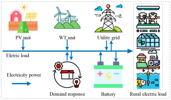
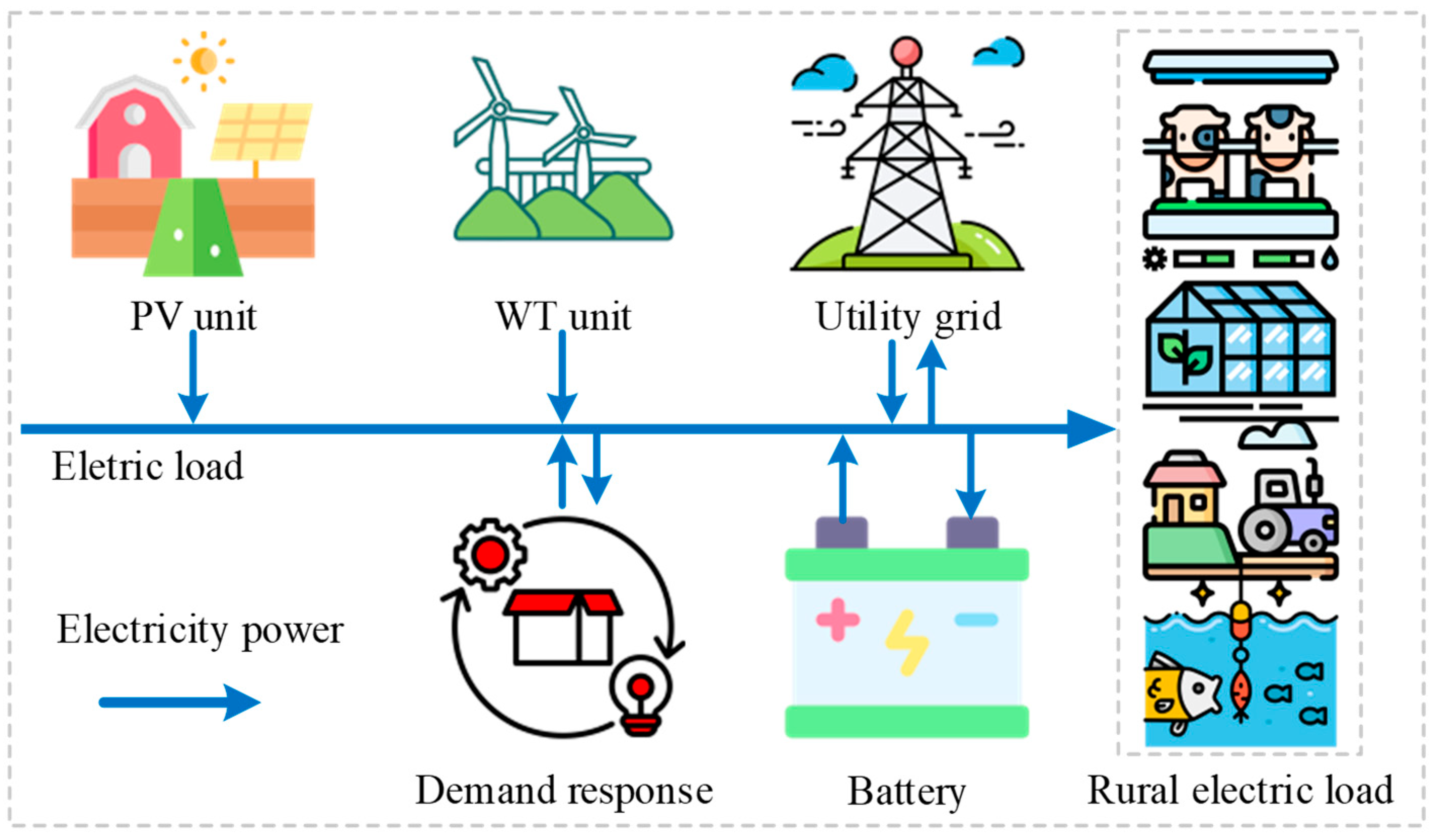
The basic structure of the rural microgrid constructed in this paper is shown in Figure 1. The energy supply units in the microgrid are distributed power sources, which include both controllable and uncontrollable types. Controllable equipment consists of the battery, while uncontrollable equipment includes WT and PV units. The rural microgrid enables the combination of multiple energy-consuming units, including greenhouse cultivation, livestock barn farming, aquaculture, agricultural production, agricultural product processing, and daily household electricity use.

Figure 1. Schematic of the rural microgrid.

In the operational model of the rural microgrid designed, wind and solar power are utilized to generate electricity for users. Meanwhile, users can participate in demand response to receive compensation offered by the microgrid. Through demand response, the microgrid can sell more electricity to the utility grid during peak consumption periods for more revenue. Furthermore, when WT and PV output exceeds electricity load demand, the microgrid sells surplus electricity to the utility grid or stores it in the battery.

Obviously, the proposed rural microgrid has similar characteristics to the integrated energy system [25]. Research on the configuration optimization of this rural microgrid will be carried out.

3. Multi-Objective Configuration Optimization Model for the Rural Microgrid

3.1. Objective Function Construction

The configuration of the rural microgrid should achieve two objective functions: the economic objective $F_1$ and the environmental objective $F_2$.

(1) Economic Objective

$$\left\{\begin{array}{l}{F}_1=\max \left\{R_{grid}+R_{load}-C_{inv}-C_{o\&m}-C_{DR}-C_{pen}\right\}\\ R_{grid}={\displaystyle \sum _{t=1}^{T_{year}}\left(c_t^{grid}\cdot P_t^{grid}\right)}\\ R_{load}={\displaystyle \sum _{t=1}^{T_{year}}\left(c_t^{load}\cdot P_t^{load}\right)}\\ C_{inv}={\displaystyle \frac{r{\left(1+r\right)}^m}{{\left(1+r\right)}^m-1}}\left(c_{inv}^{WT}\cdot N_{WT}+c_{inv}^{PV}\cdot N_{PV}+c_{inv}^{BT}\cdot N_{BT}\right)\\ C_{o\&m}=\alpha \cdot C_{inv}\\ C_{DR}={\displaystyle \sum _{t=1}^{T_{year}}\left(c_{sl}^{load}\cdot \left|P_{sl,t}^{load}\right|+c_{cl}^{load}\cdot P_{cl,t}^{load}+c_{il}^{load}\cdot P_{il,t}^{load}\right)}\\ C_{pen}=c_{pen}{\displaystyle \sum _{t=1}^{T_{year}}\left(P_t^{load,cut}\right)}\end{array}\right.$$

(1)

As shown in Equation (1), the economic objective is to maximize the annual profit of the rural microgrid, which equals the sum of the microgrid’s annual electricity sales revenue $R_{grid}$ and the revenue $R_{load}$ from serving rural electricity load, minus the microgrid’s annualized investment cost $C_{inv}$, annual operation and maintenance cost $C_{o\&m}$, rural load demand response compensation cost $C_{DR}$, and load shedding penalty cost $C_{pen}$. $c_t^{grid}$ and $P_t^{grid}$ represent the market electricity price and the amount of electricity sold from the rural microgrid at time $t$, respectively. $T_{year}$ denotes all time periods within a year. $c_t^{load}$ and $P_t^{load}$ represent the unit price of rural electricity load and the amount of electricity provided by the microgrid at time $t$, respectively. $r$ denotes the annual interest rate. $m$ represents the equipment life. $c_{inv}^{WT}$ and $N_{WT}$ denote the unit investment cost number of WT, respectively. $c_{inv}^{PV}$ and $N_{PV}$ denote the unit investment cost and the number of PV, respectively. $c_{inv}^{BT}$ and $N_{BT}$ denote the unit investment cost and the configured capacity of the battery, respectively. $\alpha$ denotes the equipment operation and maintenance coefficient. $c_{sl}^{load}$, $c_{cl}^{load}$, and $c_{il}^{load}$ represent the unit compensation cost for shiftable load, reducible load, and interruptible load demand response, respectively. $P_{sl,t}^{load}$, $P_{cl,t}^{load}$, and $P_{il,t}^{load}$ denote the shiftable load, reducible load, and interruptible load at time $t$, respectively. $c_{pen}$ and $P_t^{load,cut}$ denote the unit penalty cost for load shedding and the rural load shed at time $t$, respectively.

(2) Environmental Objective

$$\begin{array}{c}{F}_2=\max \left\{{\xi }_{C{O}_2}{\displaystyle \sum _{t=1}^{T_{year}}\left(P_t^{grid}+P_t^{load}\right)}\right\}\end{array}$$

(2)

The environmental objective is to maximize the positive externalities generated by selling green electricity from the rural microgrid; namely, the rural microgrid achieves equivalent carbon dioxide emissions reductions by replacing thermal power generation through either selling green electricity to the main grid or meeting rural load demands. The rural microgrid can generate green electricity through PV and WT output, and then sell it to the utility grid or directly provide for nearby rural areas. The generated green electricity can replace an equivalent amount of electricity generated by thermal power plants which cause carbon dioxide emissions. In other words, there is no carbon dioxide generation during the rural microgrid operating, thereby achieving an equivalent reduction in carbon dioxide emissions and obtaining environmental positive externalities. The specific expression is shown in Equation (2). The carbon dioxide emission coefficient is for thermal power units producing the same amount of electricity as the rural microgrid. ${\xi }_{C{O}_2}$ is the carbon dioxide emission factor of the thermal power unit.

3.2. Constraints Construction

(1) Equipment Capacity Configuration Constraints

$$\begin{array}{c}{N}_{WT}^{\min }\le N_{WT}\le N_{WT}^{\max }\end{array}$$

(3)

$$\begin{array}{c}{N}_{PV}^{\min }\le N_{PV}\le N_{PV}^{\max }\end{array}$$

(4)

$$\begin{array}{c}{N}_{BT}^{\min }\le N_{BT}\le N_{BT}^{\max }\end{array}$$

(5)

where $N_{WT}^{\min }$ and $N_{WT}^{\max }$ represent the lower and upper limits of the planned number of WT, respectively. $N_{PV}^{\min }$ and $N_{PV}^{\max }$ represent the lower and upper limits of the planned number of PV, respectively. $N_{BT}^{\min }$ and $N_{BT}^{\max }$ represent the lower and upper limits of the battery capacity, respectively.

(2) Operation Constraints

(a) WT

$${\widehat{p}}_t^{\mathrm{WT}}=\left\{\begin{array}{cc}0& v_t\le v_{ci},v_t>v_{co}\\ {\displaystyle \frac{v_t^3-v_{ci}^3}{v_r^3-v_{ci}^3}}{P}_r& v_{ci}<v_t<v_r\\ P_r& v_r\le v_t\le v_{co}\end{array}\right.\hspace{1em}\forall t=1,\dots ,T$$

(6)

$$\begin{array}{c}{P}_t^{WT}=\end{array}{N}_{WT}{\widehat{p}}_t^{WT}\begin{array}{cc}& \forall t=1,2,\dots ,T\end{array}$$

(7)

$$\begin{array}{c}0\le P_t^{WT,cut}\le P_t^{WT}\end{array}\begin{array}{cc}& \forall t=1,2,\dots ,T\end{array}$$

(8)

where ${\widehat{p}}_t^{\mathrm{WT}}$ represents the output of a single WT at time $t$. $P_r$ denotes the rated power of a single wind turbine. $v_t$ indicates the actual wind speed at time $t$. $v_{ci}$ and $v_{co}$ represent the cut-in and cut-out wind speed, respectively. $v_r$ signifies the rated wind speed. $P_t^{WT}$ denotes the WT output of the rural microgrid at time $t$. $P_t^{WT,cut}$ represents the curtailed WT output at time $t$.

(b) Constrains for PV

$${\widehat{p}}_t^{PV}={10}^{-3}\cdot S^{PV}\cdot cos\theta \times {\eta }^{PV}\times {\eta }^m\times r_t\begin{array}{cc}& \forall t=1,\dots ,T\end{array}$$

(9)

$$\begin{array}{c}{P}_t^{PV}=\end{array}{N}_{PV}{\widehat{p}}_t^{PV}\begin{array}{cc}& \forall t=1,2,\dots ,T\end{array}$$

(10)

$$\begin{array}{c}0\le P_t^{PV,cut}\le P_t^{PV}\end{array}\begin{array}{cc}& \forall t=1,2,\dots ,T\end{array}$$

(11)

where ${\widehat{p}}_t^{PV}$ represents the output of a single PV panel at time $t$. $S^{PV}$ denotes the area of a single PV panel. $\theta$ is the tilt angle of the PV panel. ${\eta }^{PV}$ and ${\eta }^m$ represent the efficiency of the PV. $r_t$ indicates the solar irradiance at time $t$. $P_t^{PV}$ signifies the PV output at time $t$. $P_t^{PV,cut}$ represents the curtailed PV output at time $t$.

(c) Battery

$${\Phi }_t={\Phi }_{t-1}+\left({\eta }_{ch}^{BT}\cdot P_{ch,t}^{BT}-P_{dch,t}^{BT}/{\eta }_{dch}^{BT}\right)\begin{array}{cc}& \forall t=1,\dots ,T\end{array}$$

(12)

$${\Phi }_T={\Phi }_0$$

(13)

$$0\le P_{ch,t}^{BT}\le u_{ch,t}^{BT}\cdot P_{ch}^{BT,max}\begin{array}{cc}& \forall t=1,\dots ,T\end{array}$$

(14)

$$0\le P_{dch,t}^{BT}\le u_{dch,t}^{BT}\cdot P_{dch}^{BT,max}\begin{array}{cc}& \forall t=1,\dots ,T\end{array}$$

(15)

$$0\le u_{ch,t}^{BT}+u_{dch,t}^{BT}\le 1\begin{array}{cc}& \forall t=1,\dots ,T\end{array}$$

(16)

$$\begin{array}{c}{\epsilon }_{\min }\cdot N_{BT}\le {\Phi }_t\le {\epsilon }_{\max }\cdot N_{BT}\end{array}\begin{array}{cc}& \forall t=1,2,\dots ,T\end{array}$$

(17)

$$\begin{array}{c}4\cdot \Delta t\cdot P_{ch}^{BT,\max }=N_{BT}\end{array}$$

(18)

$$\begin{array}{c}0\le P_{ch,t}^{BT}\le P_{ch}^{BT,\max }\end{array}\begin{array}{cc}& \forall t=1,2,\dots ,T\end{array}$$

(19)

$$\begin{array}{c}4\cdot \Delta t\cdot P_{dch}^{BT,\max }=N_{BT}\end{array}$$

(20)

$$\begin{array}{c}0\le P_{dch,t}^{BT}\le P_{dch}^{BT,\max }\end{array}\begin{array}{cc}& \forall t=1,2,\dots ,T\end{array}$$

(21)

where ${\Phi }_t$ represents the electricity stored in battery at time $t$. $P_{ch,t}^{BT}$ and $P_{dch,t}^{BT}$ denote the charging and discharging electricity, respectively. ${\eta }_{ch}^{BT}$ and ${\eta }_{dch}^{BT}$ indicate the charging and discharging efficiency, respectively. ${\epsilon }_{\min }\cdot$ and ${\epsilon }_{\max }$ denote the minimum and maximum power coefficients, respectively. ${\Phi }_0$ and ${\Phi }_T$ represent the stored electricity at the start and end of a day, respectively, which ensure the cyclic utilization of electricity. $u_{ch,t}^{BT}$ and $u_{dch,t}^{BT}$ denote the charging and discharging states, respectively, which are 0–1 variables. $P_{ch}^{BT,max}$ and $P_{dch}^{BT,max}$ represent the rated charging and discharging power.

(d) Demand Response

This paper categorizes rural electricity loads into two main types: adjustable load (AL) and non-adjustable load (NAL) [26]. NAL refers to loads with great political and economic significance, or that would cause significant losses, safety incidents and impact users’ production and daily life without this type of load. AL refers to loads that users can independently adjust based on electricity prices and incentive policies without inconveniencing their daily live. AL includes shiftable load, reducible load, and interruptible load.

$$P_t^{load}=P_{nal,t}^{load}+P_{al,t}^{load}\begin{array}{cc}& \forall t=1,\dots ,T\end{array}$$

(22)

$$P_{al,t}^{load}=r^{al}\cdot {\widehat{P}}_t^{load}+P_{sl,t}^{load}-P_{cl,t}^{load}-P_{il,t}^{load}\begin{array}{cc}& \forall t=1,\dots ,T\end{array}$$

(23)

$$-r^{al}\cdot {\widehat{P}}_t^{load}\le P_{sl,t}^{load}-P_{cl,t}^{load}-P_{il,t}^{load}\le r^{al}\cdot {\widehat{P}}_t^{load}\begin{array}{cc}& \forall t=1,\dots ,T\end{array}$$

(24)

$$r^{sl}+r^{cl}+r^{il}=1\begin{array}{cc}& \forall t=1,\dots ,T\end{array}$$

(25)

$${{\displaystyle \sum }}_{t=1}^T{P}_{sl,t}^{load}=0$$

(26)

$$-r^{sl}\cdot P_{al,t}^{load}\le P_{sl,t}^{load}\le r^{sl}\cdot P_{al,t}^{load}\begin{array}{cc}& \forall t=1,\dots ,T\end{array}$$

(27)

$$0\le P_{cl,t}^{load}\le r^{cl}\cdot P_{al,t}^{load}\begin{array}{cc}& \forall t=1,\dots ,T\end{array}$$

(28)

$$0\le {{\displaystyle \sum }}_{t=1}^T{P}_{il,t}^{load}\le r^{il}{{\displaystyle \sum }}_{t=1}^T{P}_{al,t}^{load}$$

(29)

where $P_t^{load}$ represents the actual rural electricity load. ${\widehat{P}}_t^{load}$ represents the forecasted rural electricity load. $P_{nal,t}^{load}$ and $P_{al,t}^{load}$ represent the NAL and AL, respectively. $P_{sl,t}^{load}$, $P_{cl,t}^{load}$, and $P_{il,t}^{load}$ denote the shiftable, reducible, and interruptible load, respectively. $r^{al}$ is the proportion of AL relative to the total forecasted load. $r^{sl}$, $r^{cl}$, and $r^{cl}$ represent the proportions of shiftable load, reducible load, and interruptible load relative to the AL, respectively.

(e) Load Shedding and Node Balance

$$\begin{array}{c}0\le P_t^{load,cut}\le P_t^{load}\end{array}\begin{array}{cc}& \forall t=1,2,\dots ,T\end{array}$$

(30)

$$\begin{array}{c}\left(P_t^{WT}-P_t^{WT,cut}\right)+\left(P_t^{PV}-P_t^{PV,cut}\right)+P_{dch,t}^{BT}\end{array}=P_t^{grid}+\left(P_t^{load}-P_t^{load,cut}\right)+P_{ch,t}^{BT}\begin{array}{cc}& \forall t=1,2,\dots ,T\end{array}$$

(31)

The above objective functions and constraints constitute the multi-objective configuration optimization model for the rural microgrid.

4. Model Solving

4.1. Multi-Objective Weighting Based on Shapley Value Method

The weight of economic objective and environmental objective in the total objective is determined using the Shapley value method [27]:

$$A_k={{\displaystyle \sum }}_{j\in f}\delta \left(\left|f\right|\right)\left[A\left(f\right)-A\left(f\backslash k\right)\right],k=1,2$$

(32)

$$\delta \left(\left|f\right|\right)={\displaystyle \frac{\left(N-\left|f\right|\right)!\left(\left|f\right|-1\right)!}{N!}}$$

(33)

where $\mathrm{f}$ denotes any subset of the objective function set. $\left|\mathrm{f}\right|$ represents the number of objective functions in the subset. $\mathsf{\delta }\left(\left|\mathrm{f}\right|\right)$ is the weighting coefficient, which indicates the objective weight of a specific objective function in the total objective. $\mathrm{k}$ is an index denoting a particular objective function in the Shapley combination. $\mathrm{A}\left(\mathrm{f}\right)$ denotes the function value of subset $\mathrm{f}$. $\mathrm{A}\left(\mathrm{f}\backslash \mathrm{k}\right)$ represents the function value achievable in subset $\mathrm{f}$ after removing the $\mathrm{k}$-th benefit indicator. ${\mathrm{A}}_{\mathrm{k}}$ is the error quantity assigned to objective function $\mathrm{k}$, i.e., the Shapley value.

Furthermore, based on Equations (32) and (33), the weights ${\mathsf{\omega }}_1$ and ${\mathsf{\omega }}_2$ correspond to each objective function using the following formula:

$${\omega }_1={\displaystyle \frac{1}{4-1}}·{\displaystyle \frac{A-A_1}{A}}$$

(34)

$${\omega }_2={\displaystyle \frac{1}{4-1}}·{\displaystyle \frac{A-A_2}{A}}$$

(35)

where $\mathrm{A}$ is the sum of Shapley value allocations.

To clarify the applicability and superiority of the Shapley value method in multi-objective weighting, this paper theoretically compares it with two types of mainstream multi-objective processing methods:

Comparison with the traditional weighted sum method. The traditional weighted sum method usually presets fixed weights or assigns weights subjectively according to the decision-maker’s preferences. The weight setting of such methods lacks objective basis and is difficult to reflect the real game relationship between objectives. In addition, linear weighting implies the assumption that objectives are completely substitutable, which is inconsistent with the nonlinear trade-off relationship between objectives in actual decision-making. In contrast, the Shapley value method is based on cooperative game theory, and determines weights by calculating the marginal contribution of each objective function in all possible objective alliances, realizing the endogenization and objectivity of weights. This method can capture the cooperative and competitive relationships between objectives, making the weight allocation more in line with the essence of multi-objective optimization problems.

Comparison with the Pareto multi-objective optimization method. Although Pareto frontier methods (such as NSGA-II) can generate a set of non-dominated solutions, decision-makers still need to select an optimal compromise solution from them, and the selection process still relies on subjective judgment or external criteria. In addition, in the high-dimensional objective space, the distribution of the Pareto solution set is often sparse, which increases the difficulty of decision-making. The Shapley value method directly outputs a uniquely determined optimal solution by converting multiple objectives into a single comprehensive objective, avoiding the subjectivity of subsequent decisions, and is more suitable for scenarios in engineering practice that require clear configuration schemes. At the same time, the Shapley value method retains the game information between objectives, and its weights can be interpreted as the contribution of each objective to the comprehensive benefit, providing decision-makers with a transparent and traceable decision basis.

Comparison with the ideal point method. Ideal point methods (such as TOPSIS) need to first define positive ideal solutions and negative ideal solutions, and calculate the distance between each scheme and the ideal solution. Their results are sensitive to the selection of ideal solutions, and it is difficult to handle the correlation between objectives. The Shapley value method does not rely on external benchmarks, and allocates weights completely based on the internal relationship of objective function values, which has stronger data-driven characteristics and robustness.

Although the Shapley value method exhibits the above advantages in multi-objective weighting, its application still has certain prerequisites and limitations:

(1) The objective function values need to be comparable, that is, each objective should be normalized to the same dimension or order of magnitude.

(2) There should be a certain cooperative game relationship between objectives, that is, each objective is neither completely consistent nor completely opposed.

(3) The calculation of the Shapley value requires traversing all objective subsets, and the computational complexity increases exponentially when the number of objectives is large.

To evaluate the impact of the above limitations on the research conclusions, the robustness of the weight allocation and optimization results under the fluctuation of objective function values will be investigated through sensitivity analysis in the following section.

4.2. Model Solving Based on the Global Harmony Search Algorithm

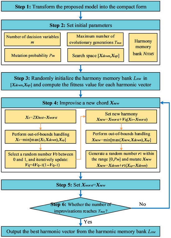
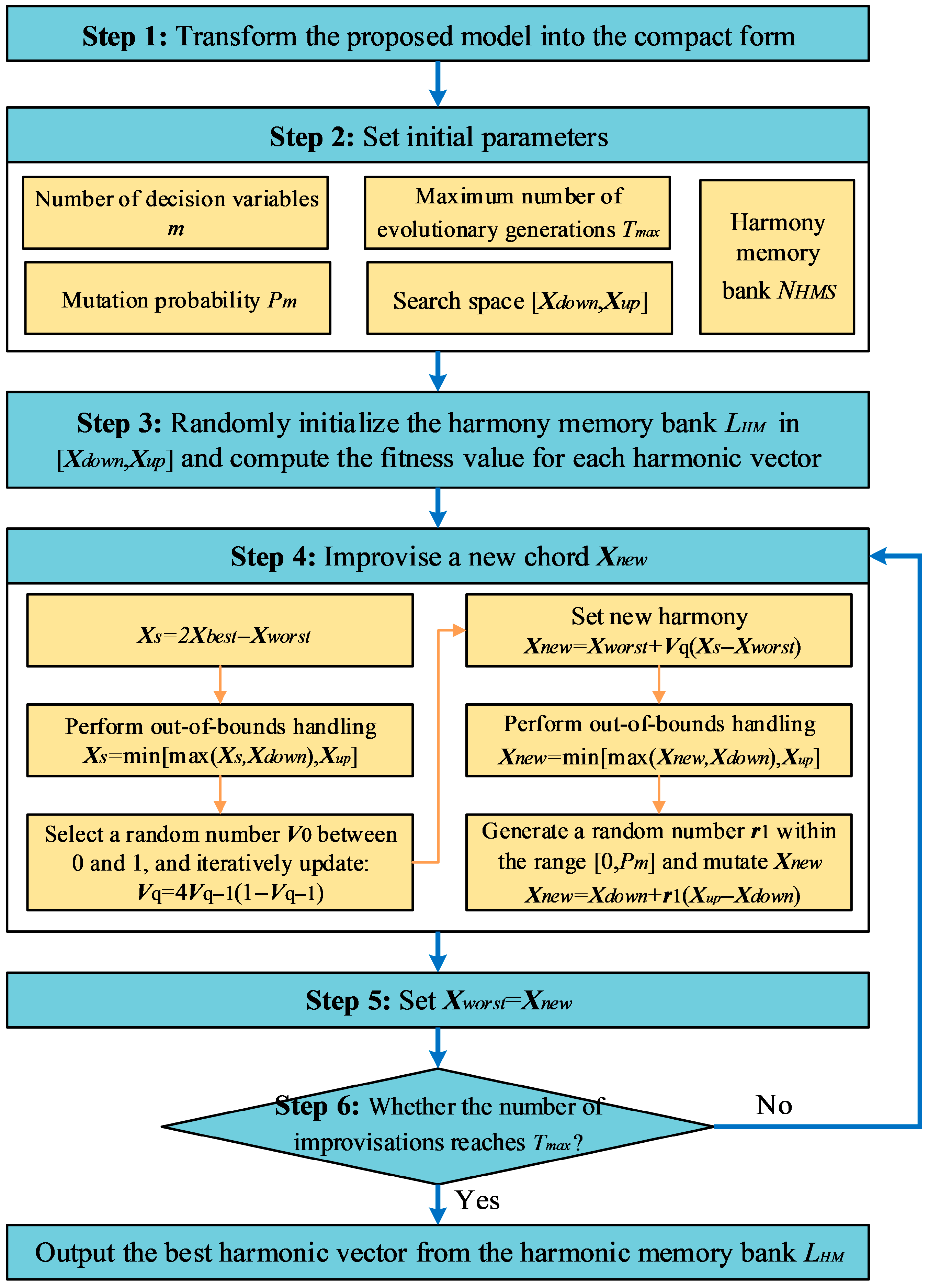
This paper employs the harmonic search algorithm for solving the model. The traditional harmonic search algorithm often experiences the stagnation phenomenon. By replacing the pitch fine-tuning operation of the traditional harmonic search algorithm with the position update and low-probability mutation approach, a GHS algorithm is formed. The specific solution steps of GHS are as follows:

Step 1: Transform the proposed model into the following compact form:

$$\left\{\begin{array}{c}minf\left(\mathit{X}\right)\\ \mathit{X}\in \left[{\mathit{X}}_{down},{\mathit{X}}_{up}\right]\end{array}\right.$$

(36)

where $\mathrm{f}\left(\mathrm{X}\right)$ is the objective function, $\mathrm{X}$ is the solution vector composed of decision variables, i.e., the harmonic vector. ${\mathrm{X}}_{\mathrm{low}}$ denotes the lower bound of the decision variables, and ${\mathrm{X}}_{\mathrm{up}}$ denotes the upper bound.

Step 2: Set initial parameters, including the number of decision variables $\mathrm{m}$, maximum number of evolutionary generations ${\mathrm{T}}_{\max }$, mutation probability ${\mathrm{P}}_{\mathrm{m}}$, search space [${\mathrm{X}}_{\mathrm{down}},{\mathrm{X}}_{\mathrm{up}}$] for each decision variable, as well as the size ${\mathrm{N}}_{\mathrm{HMS}}$ of the harmonic memory store.

Step 3: Randomly initialize the harmony memory bank ${\mathrm{L}}_{\mathrm{HM}}$ in the search space and compute the fitness value for each harmonic vector.

Step 4: Improvise a new chord ${\mathrm{X}}_{\mathrm{new}}$. Specifically:

(1) Firstly, let ${\mathrm{X}}_{\mathrm{s}}=2{\mathrm{X}}_{\mathrm{best}}-{\mathrm{X}}_{\mathrm{worst}}$, where ${\mathrm{X}}_{\mathrm{best}}$ and ${\mathrm{X}}_{\mathrm{worst}}$ represent the best and worst harmonies in the harmonic memory bank ${\mathrm{L}}_{\mathrm{HM}}$, respectively.

(2) Next, perform out-of-bounds handling for ${\mathrm{X}}_{\mathrm{s}}$:

$${\mathit{X}}_s=\min \left[\max \left({\mathit{X}}_s,{\mathit{X}}_{donw}\right),{\mathit{X}}_{up}\right]$$

(37)

(3) Select a random number ${\mathrm{V}}_0$ between 0 and 1 as the initial position point, and iteratively update the position point according to Equation (38):

$${\mathit{V}}_q=4{\mathit{V}}_{q-1}\left(1-{\mathit{V}}_{q-1}\right)$$

(38)

where $\mathrm{q}$ denotes the number of evolutionary iterations.

(4) Set new harmony ${\mathrm{X}}_{\mathrm{new}}={\mathrm{X}}_{\mathrm{worst}}+{\mathrm{V}}_{\mathrm{q}}\left({\mathrm{X}}_{\mathrm{s}}-{\mathrm{X}}_{\mathrm{worst}}\right)$.

(5) Perform out-of-bounds handling for ${\mathrm{X}}_{\mathrm{new}}$:

$${\mathit{X}}_{new}=\min \left[\max \left({\mathit{X}}_{new},{\mathit{X}}_{donw}\right),{\mathit{X}}_{up}\right]$$

(39)

(6) Generate a random number ${\mathrm{r}}_1$ within the range [0, ${\mathrm{P}}_{\mathrm{m}}$], and mutate ${\mathrm{X}}_{\mathrm{new}}$ based on Formula (40):

$${\mathit{X}}_{new}={\mathit{X}}_{donw}+r_1\left({\mathit{X}}_{up}-{\mathit{X}}_{donw}\right)$$

(40)

Step 5: Set ${\mathrm{X}}_{\mathrm{worst}}={\mathrm{X}}_{\mathrm{new}}$.

Step 6: If the number of improvisations reaches the maximum evolutionary iteration number ${\mathrm{T}}_{\max }$, terminate and output the best harmonic vector from the harmonic memory bank. Otherwise, return to Step 4 and proceed to create a new harmony ${\mathrm{X}}_{\mathrm{new}}$.

The solution process for the GHS algorithm is shown in Figure 2.

Figure 2. Flow chart of GHS algorithm.

5. Simulation

5.1. Data Descriptions

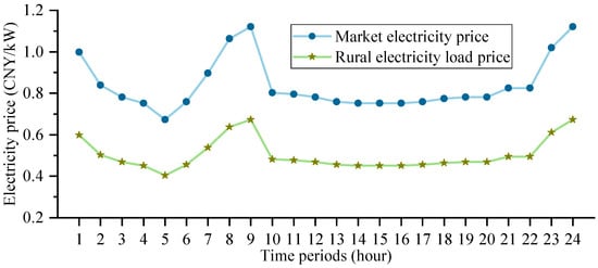
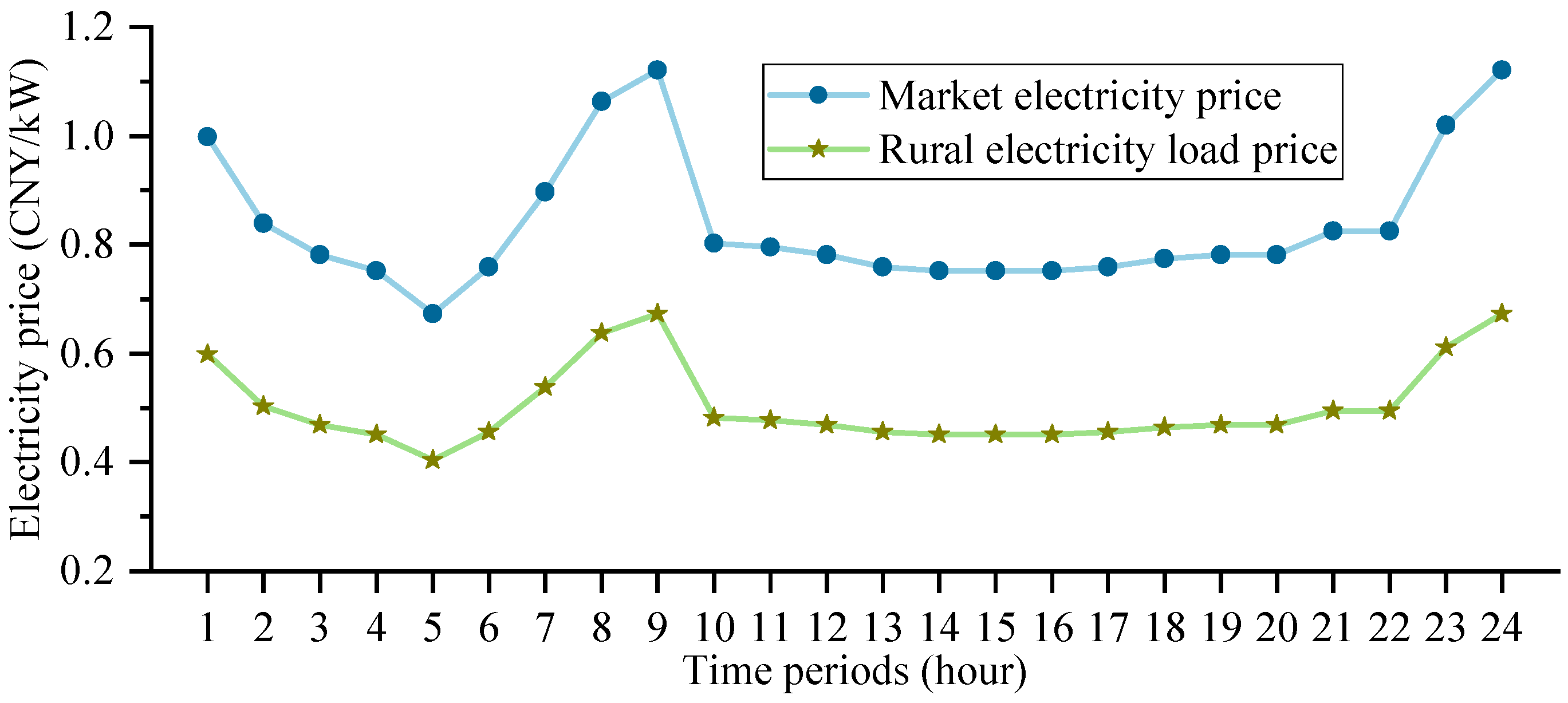
A rural microgrid was allocated to a village in North China. This region has abundant solar and wind energy resources. The basic parameters for the microgrid construction and operation are shown in Table 2, and other technical parameters of the rural microgrid are listed in Table 3. The market electricity price and rural electricity load pricing for this region are illustrated in Figure 3 [28].

Table 2. Construction and operation parameters of the rural microgrid.

Parameter	Value	Unit	Ref	Parameter	Value	Unit	Ref
$c_{inv}^{WT}$	28,891	$	[29]	$m$	20	years	[30]
$c_{inv}^{PV}$	433	$	[29]	$r$	7%	/	[30]
$c_{inv}^{BT}$	361	$/kWh	[31]	$\alpha$	0.02	/	[30]

Table 3. Other technical parameters of the rural microgrid.

Parameter	Value	Unit	Ref	Parameter	Value	Unit	Ref
$N_{WT}^{\min }$$/N_{WT}^{\max }$	1/20	/	[29]	${\eta }_{ch}^{BT}$$/{\eta }_{dch}^{BT}$	0.9/0.9	/	[31]
$N_{PV}^{\min }$$/N_{PV}^{\max }$	1000/10,000	/	[29]	$r^{al}$	30%	/	[32]
$N_{BT}^{\min }$$/N_{BT}^{\max }$	1000/12,000	kWh	[31]	${\epsilon }_{\min }$$/{\epsilon }_{\max }$	0.05/0.95	/	[32]
$P_r$	500	kW	[29]	$r^{sl}$$/r^{cl}$$/r^{il}$	60%/20%/20%	/	[32]
$v_{ci}$$/v_{co}$$/v_r$	3/27/8	m/s	[29]	$c_{sl}^{load}$$/c_{cl}^{load}$$/c_{il}^{load}$	0.0144/0.0217/ 0.0217	$/kW	[32]
$S^{PV}$	2	m2	[30]	$c_{pen}$	5	$/kW	[33]
$\theta$	60	/	[30]	${\xi }_{C{O}_2}$	0.6101	kg/kW	[30]
${\eta }^{PV}$$/{\eta }^m$	0.5/0.96	/	[30]

Figure 3. Market electricity price and rural electricity load price.

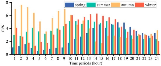
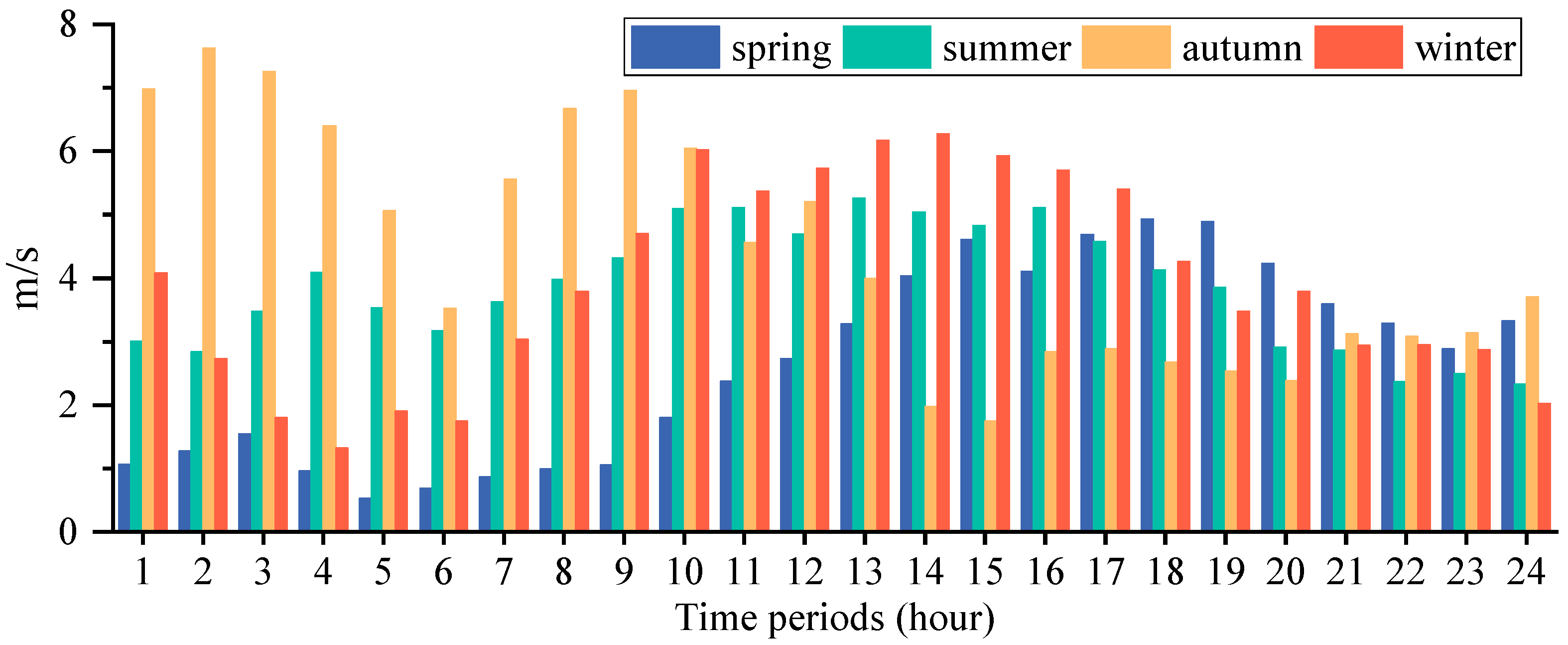
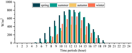
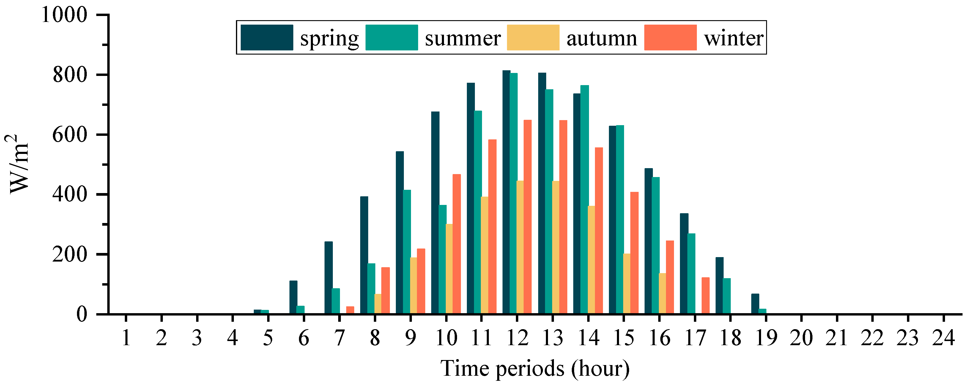
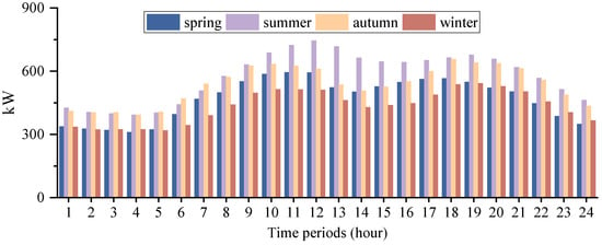
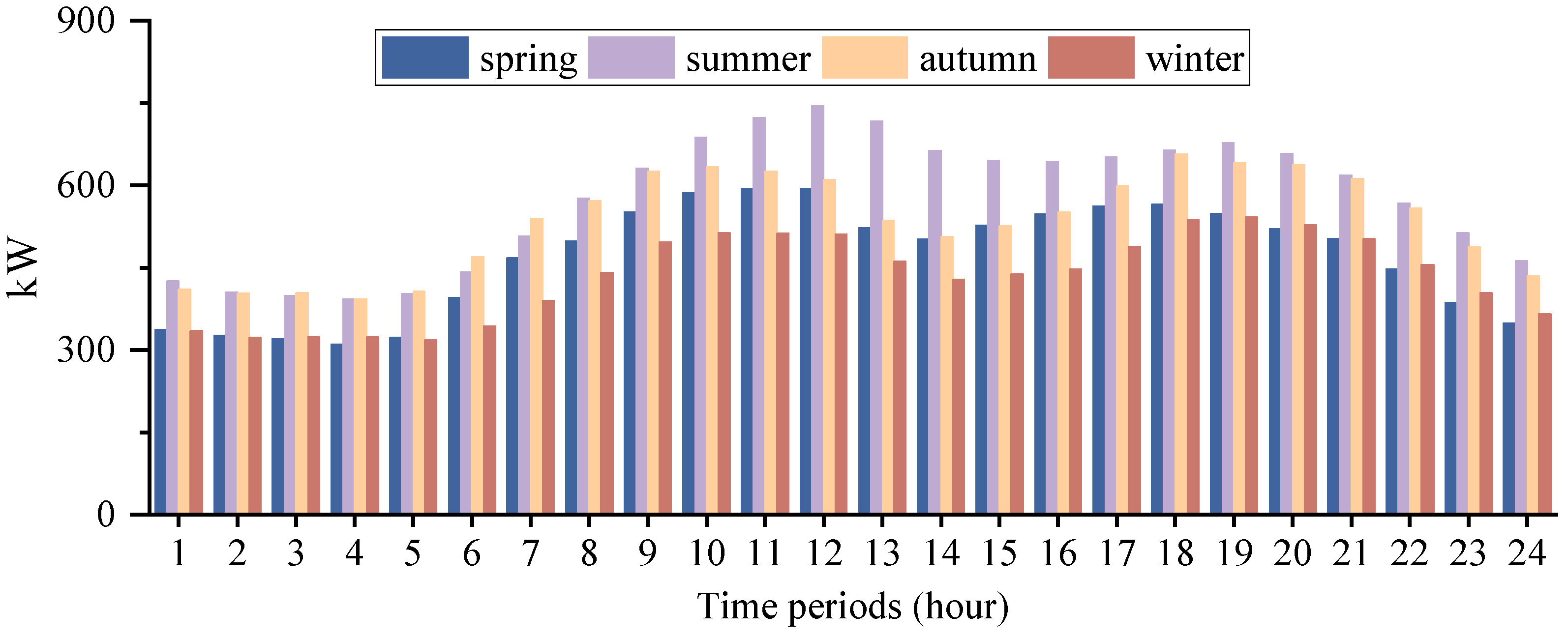
This study investigates the optimization of rural microgrid configurations over a one-year cycle, encompassing 365 days in total. Simulation calculations were performed using typical daily wind speeds, solar irradiance, and electricity load data from four representative seasonal days. The typical daily wind speeds, solar irradiance, and rural electricity load data are shown in Figure 4, Figure 5 and Figure 6, respectively. The specific considerations for selecting these four typical seasonal days are as follows:

Figure 4. Typical daily wind speed.

Figure 5. Typical daily solar radiation.

Figure 6. Typical daily rural electricity load.

(1) Typicality of meteorology and load. The wind speed, solar irradiance, and load curves of the selected typical days are all obtained from the cluster analysis of historical and actual measurement data (2024) in the region. Their daily average wind speed, solar irradiance, and load are close to the average values of each corresponding season, which can be regarded as the average scenario of that season.

(2) Applicability in the planning stage. In the long-term capacity configuration optimization, the adoption of typical days can significantly reduce the model complexity and computational burden while still capturing the most significant differences in resources and demands between seasons. This method has been widely verified to be effective in similar studies [34,35].

This paper uses MATLAB R2023a software to solve the optimization problem with Intel Core i7-12700H, 1.80 GHz CPU and 16 GB memory.

5.2. Analysis of Optimization Result Using Shapley Value Method and GHS Algorithm

5.2.1. Analysis of Weighting Result Based on the Shapley Value Method

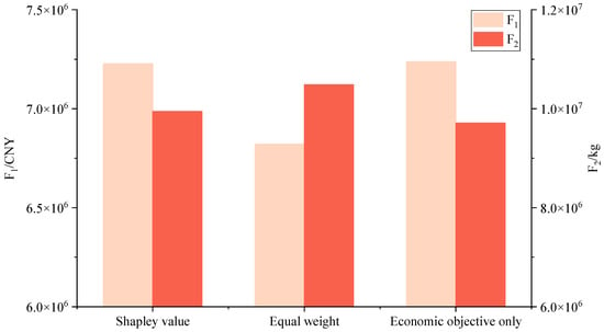
According to Equations (32)–(35), the weights of ${\mathrm{F}}_1$ and ${\mathrm{F}}_2$ in this paper are calculated as ${\mathsf{\omega }}_1$ = 0.68 and ${\mathsf{\omega }}_2$ = 0.32, respectively. To validate the advantage of Shapley value method weighting, this section compares the ${\mathrm{F}}_1$ and ${\mathrm{F}}_2$ values obtained using Shapley value method weighting, equal weighting, and an economic-only objective function, as shown in Figure 7.

Figure 7. Comparison of ${\mathrm{F}}_1$ and ${\mathrm{F}}_2$ values through different objective function weighting methods.

As shown in Figure 7, comparing the Shapley value weighting method with the equal weighting approach, the latter achieves equivalent carbon reductions of 540.70 tons at the cost of sacrificing $ 5.86 × 10⁴ in economic revenue. Analyzing the ratio, economic revenue decreased by 5.62% relative to the former method, while environmental benefits increased by 5.44%. It seems that when economic and environmental objectives are equally weighted, the environmental improvement achieved is insufficient to offset the economic decline, failing to provide decision-makers with the most valuable decision support.

Comparing the Shapley value weighting method when only considering the economic objective function (i.e., economic objective weighted at 1), the latter achieves an economic revenue increase of $ 1.46 × 10³ by sacrificing 233.39 tons of equivalent carbon emission reductions. Analyzing the ratio, the environmental benefit decrease by 2.35% compared to the former, while the economic revenue increases by 0.14%. Thus, when considering only the economic objective, the gained economic revenue is insufficient to offset the decline in environmental benefit, failing to provide decision-makers with optimal support.

To sum up, the differentiated weighting corresponding to these two objectives obtained from the Shapley value method proposed herein ensures a balanced solution that accounts for both economic gains and environmental benefits, thus demonstrating greater rationality.

5.2.2. Optimization Result Analysis of the GHS Algorithm

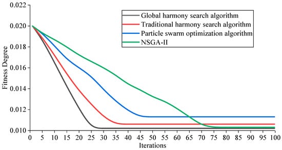
Based on the parameters set in Table 4, the GHS was applied to solve the single-objective model. To validate the superiority of the GHS algorithm, the traditional harmony search algorithm, particle swarm optimization and Non-dominated Sorting Genetic Algorithm II (NSGA-II) are employed as comparative methods. The parameters of NSGA-II are set as follows: the population size is 100, the crossover probability is 0.9, the mutation probability is 0.1, and the maximum number of evolutionary generations is 100. The iterative processes of the three algorithms are illustrated in Figure 8.

Table 4. Parameter of global harmony search algorithm.

Parameter	Value
$T_{max}$	100
$N_{HMS}$	20
$P_m$	0.05

Figure 8. The iterative processes of three algorithms.

As shown in Figure 8, the GHS algorithm converged the fastest, achieving convergence after only 25 iterations. This outperformed the 34 iterations required by the traditional harmonic search algorithm and the 45 iterations needed by the particle swarm optimization algorithm, demonstrating a significant improvement in computational efficiency. As can be seen from Figure 8, the GHS algorithm achieves the fastest convergence speed, converging after 25 iterations, which outperforms the traditional harmony search algorithm (34 iterations), the particle swarm optimization algorithm (45 iterations) and NSGA-II (71 iterations). This indicates that the computational efficiency of the global harmony search algorithm is significantly higher than that of the other three methods. In addition, the GHS algorithm proposed in this paper can significantly improve the computational efficiency while maintaining a high convergence accuracy consistent with NSGA-II, making it more suitable for the optimal configuration problem of the rural microgrid with multiple scenarios and multiple constraints and easy to be popularized and applied in practical engineering.

5.3. Analysis of Optimal Configuration Result

With the GHS algorithm solving, the final optimal configuration result for each equipment in the rural microgrid is shown in Table 5. The benefits, costs, and equivalent carbon reduction results are shown in Table 6. And the technical and economic results under optimal configuration of this rural microgrid project are listed in Table 7. Among them, the calculation formulas for the indicators of investment payoff period (IPP) and internal rate of return (IRR) are given in Equations (41) and (42).

$${\displaystyle \sum _{k=1}^{IPP}\frac{C{F}_k}{{\left(1+r\right)}^k}}=C_0$$

(41)

$$NPV={\displaystyle \sum _{k=1}^m\frac{C{F}_k}{{\left(1+IRR\right)}^k}}=0$$

(42)

where $C_0$ denotes the initial investment cost of the project. $C{F}_k$ represents the net cash flow in the k-th year. $r$ denotes the annual interest rate. $NPV$ means the net present value. $m$ represents the equipment life.

Table 5. Configuration results of equipment capacity.

Device	Capacity	Unit
WT	10,000	kW
PV	4800	kW
BT	7436	kWh

Table 6. Benefit, cost and equivalent carbon emission reduction results under optimal configuration.

Parameter	Result	Unit
Annual revenue from selling electricity to utility grid	1.49 × 106	$
Annual revenue from rural power load	3.02 × 105	$
Annual construction cost	7.17 × 105	$
Annual operation and maintenance cost	1.43 × 104	$
Annual demand response compensation cost	1.40 × 104	$
Annual penalty cost of load shedding	0	$
Annual equivalent carbon emission reduction	9.94 × 104	t

Table 7. Technical and economic results under optimal configuration.

Parameter	Result	Unit
Annual revenue	1.76 × 106	$
IPP	5.32	year
IRR	23.04%	/

As shown in Table 5 and Table 6, the final configuration for the rural microgrid includes 20 WT with a total capacity of 10,000 kW, 10,000 PV covering an area of 20,000 square meters, and a battery capacity of 7436 kWh. Under the optimal configuration, the annual construction cost of the rural microgrid is 7.17 × 10⁵ $, the annual operation and maintenance cost is 1.43 × 10⁴ $, the annual demand response compensation cost is 1.40 × 10⁴ $, the annual penalty cost for electricity load shedding is 0 $, and the annual equivalent carbon emissions reduction is 9.94 × 10⁴ tons. It is evident that both WT and PV reached their maximum planned capacity. This is because, on the one hand, deploying larger-capacity units ensures that their output fully meets the local electricity load, thereby avoiding substantial load shedding penalty costs. On the other hand, after meeting the electricity load demand, the surplus WT and PV output can be sold to the utility grid to obtain substantial electricity sales revenue. Furthermore, selling as much green electricity as possible to the utility grid can equivalently reduce more carbon emissions from the power system. Therefore, it is reasonable for the planned number of WT and PV to reach their upper limits.

The construction period for this rural microgrid project is one year, with a total construction cost of 7.60 × 10⁶ $. Upon completion, it will enter direct operation with a 20-year operating period. As shown in Table 6 and Table 7, simulation of the microgrid operation indicates an annual revenue of 1.76 × 10⁶ $ with an annual interest rate of 7%, an investment payback period of 5.32 years, and an internal rate of return of 23.04%, which is significantly greater than the annual interest rate. Therefore, the constructed rural microgrid can achieve profitability and recover all initial investment costs within an acceptable timeframe, demonstrating sustainable operational and developmental potential.

5.4. Analysis of Microgrid Operation Under Optimal Configuration

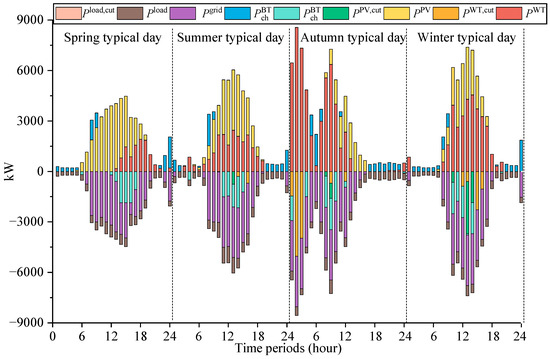
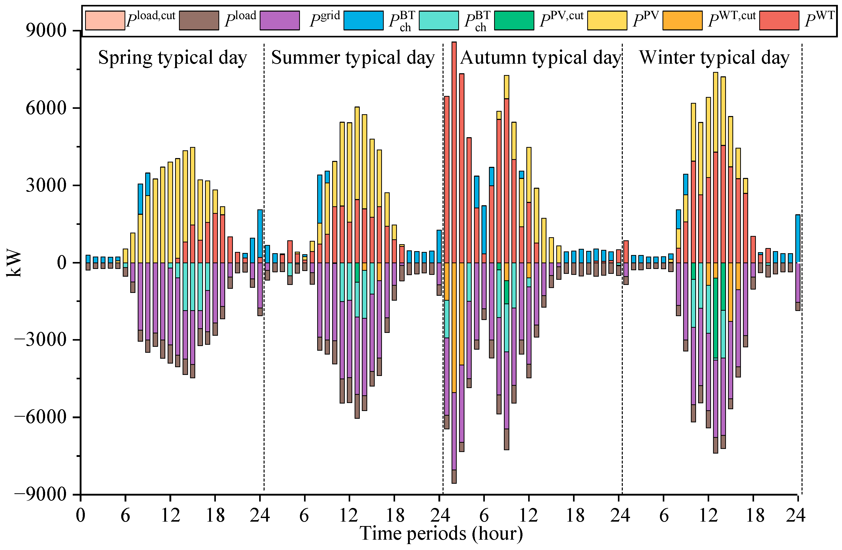
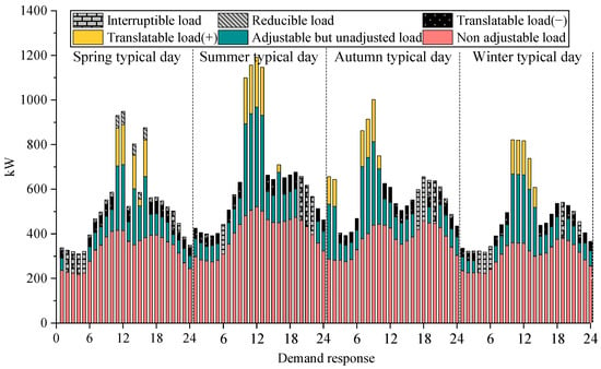
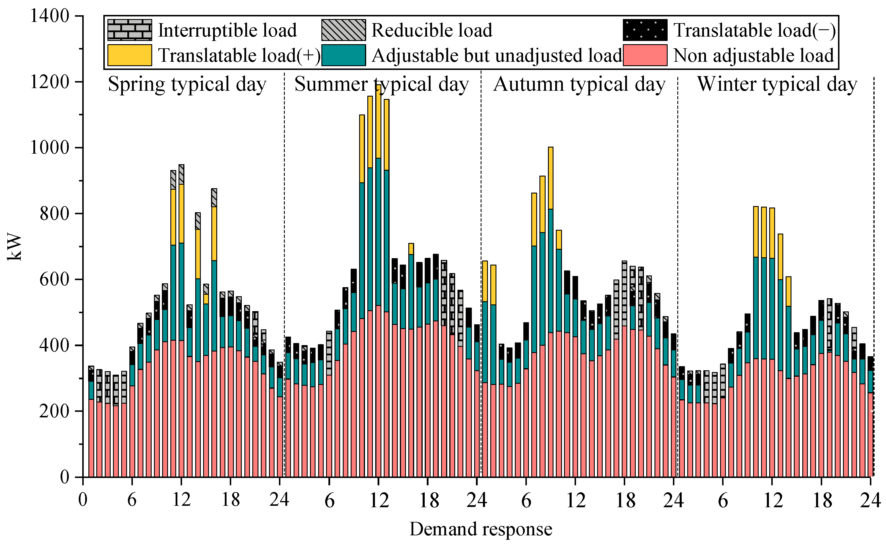
Under the optimal configuration results, four typical daily scenarios representing the seasons of spring, summer, autumn, and winter are selected for scheduling the rural microgrid. The optimal scheduling result is shown in Figure 9, and the load demand response result is presented in Figure 10. Moreover, the daily revenue and daily cost of the rural microgrid under typical daily conditions are listed in Table 8.

Figure 9. Electric node balance on different typical days.

Figure 10. Demand response on different typical days.

Table 8. Benefit and cost of rural microgrid in typical days.

Parameter	Typical Day
	Spring	Summer	Autumn	Winter
Daily revenue from selling electricity to utility grid/$	3890.60	3844.14	4793.92	26,165.36
Daily revenue from rural power load/$	744.27	944.80	898.62	3779.74
Daily demand response compensation cost/$	40.90	41.06	38.94	32.07
Daily penalty cost of load shedding/$	0	0	0	0

As shown in Figure 9, both PV and WT outputs are large on a typical day. When solar irradiation is present and wind speed exceeds the wind turbine’s cut-in speed, the excess green power from PV and WT, after meeting the rural electric load, is sold to the utility grid for profit (including economic and environmental profit). In particular, during hours 8–13, more electricity is sold to the utility grid. This is because market electricity price is relatively high (as shown in Figure 3) and consequently selling more electricity during these time periods increases microgrid revenue. It should be noted that PV and WT output are not entirely used to meet electricity load or for sales. Instead, during periods of high solar irradiation or wind speeds, a portion is stored in the battery. When PV and WT output is insufficient or electricity load is high, the battery discharges to meet the load and avoid load shedding.

As shown in Figure 10, the user participates in demand response during each time period of the typical spring day, which means users receive demand response compensation. Positive shiftable load appears during the 11–12 and 14–16 time periods while negative shiftable load, interruptible load, and curtailable load appear during the other periods. The reason for this phenomenon is that, from the user perspective, the increase in electricity consumption when rural electricity load price is relatively low and the reduction in electricity consumption during other periods can reduce users’ electricity costs. From the microgrid perspective, when both the market electricity price and rural electricity load price are high, the reduced electricity demand allows PV and WT output to be sold more extensively to the electricity market, thereby getting more revenue.

As shown in Table 8, during typical days across the four seasons, the revenue obtained from selling electricity to the utility grid during the autumn typical day is clearly higher than that of other seasonal typical days. This is because the autumn typical day has higher wind speeds and the longest duration exceeding the cut-in wind speed, enabling the rural microgrid to generate more green electricity for sale. The rural microgrid obtains the highest rural electricity load supplying revenue during the typical summer day, followed by autumn, spring, and the lowest in winter. This correlates with seasonal variations in rural electricity load patterns: high temperatures in summer drive higher load requirements, while winter’s colder conditions result in significantly lower load requirements. Demand response compensation cost incurred by the rural microgrid across the four typical days show minimal variation, which indicates users can effectively participate in load demand response and achieve benefits throughout all four seasons. Finally, the penalty cost is zero on all four typical days. This demonstrates that the rural microgrid can supply all rural electricity loads in the area without load shedding, thereby ensuring its power supply reliability.

In summary, on the one hand, the rural microgrid can fully utilize clean solar and wind energy through the synergy of its own equipment (including the WT, PV, and battery). This enables reliable power supply while selling surplus green electricity to the utility grid to generate additional revenue. On the other hand, by incentivizing user participation in electricity load demand response, the rural microgrid can promote renewable energy consumption, with a positive outcome for both users and the microgrid.

5.5. Sensitivity Analysis

(1) Potential impact of variability within each season

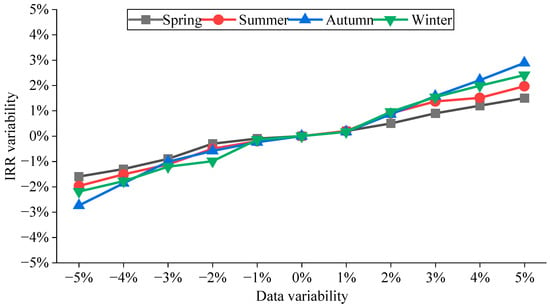
To evaluate the potential impact of variability in wind speed, solar irradiance, and electrical load data of the four selected typical days on the rural microgrid planning results, this subsection takes the IRR index of the planning results under the typical days as the benchmark, and analyzes the changes in the IRR of the microgrid planning results under the data variability of typical days in different seasons, as shown in Figure 11.

Figure 11. Changes in IRR under data variability of typical days in different seasons.

As shown in Figure 11, on the whole, with the variability in wind speed, solar irradiance, and electrical load data within the range of [−5%, 5%], the variability range of the IRR of the rural microgrid is controlled within ±3%. In particular, when the wind speed, solar irradiance, and electrical load data fluctuate within the range of [−1%, 1%], the variation rate of the IRR is close to 0%, indicating that the rural microgrid exhibits favorable robustness within this reasonable variability range. Moreover, the variability amplitude of IRR presents a regular characteristic of changing from negative to positive as the data variability amplitude increases from small to large. Specifically, comparing the data variability of typical days in each season, the data variability in autumn has the greatest impact on IRR, mainly due to its superior wind resource and load matching characteristics, followed by winter, while the impacts in summer and spring are relatively small.

(2) Electricity market price volatility

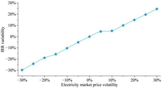
To evaluate the potential impact of electricity market price volatility on the rural microgrid planning results, this subsection takes the simulated market electricity price (as shown in Figure 3) as the benchmark, and analyzes the variations in the IRR of microgrid planning results under the volatility of the benchmark electricity price, as illustrated in Figure 12.

Figure 12. Changes in IRR under electricity market price variability.

As shown in Figure 12, the IRR is highly sensitive to the market electricity price. A ±30% fluctuation in the electricity price leads to a variation in IRR from −29.77% to +24.65%, and the impact of negative shocks is greater than that of positive gains. This is because the construction cost of the rural microgrid increases stepwise with the rise in electricity price, reflecting that the optimization model tends to expand the installed capacity when the expected revenue improves. Furthermore, the sensitivity exhibits a piecewise characteristic, and a 10% electricity price increase is the critical threshold to trigger the capacity expansion decision. Overall, the market electricity price is an important sensitive factor affecting the economy of rural microgrids. In investment decision-making, close attention should be paid to the downside risk of electricity price, and appropriately expanding the installed capacity can be considered to capture excess returns when the expected electricity price increases by more than 10%.

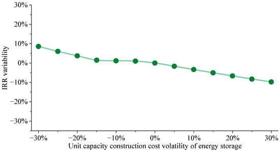
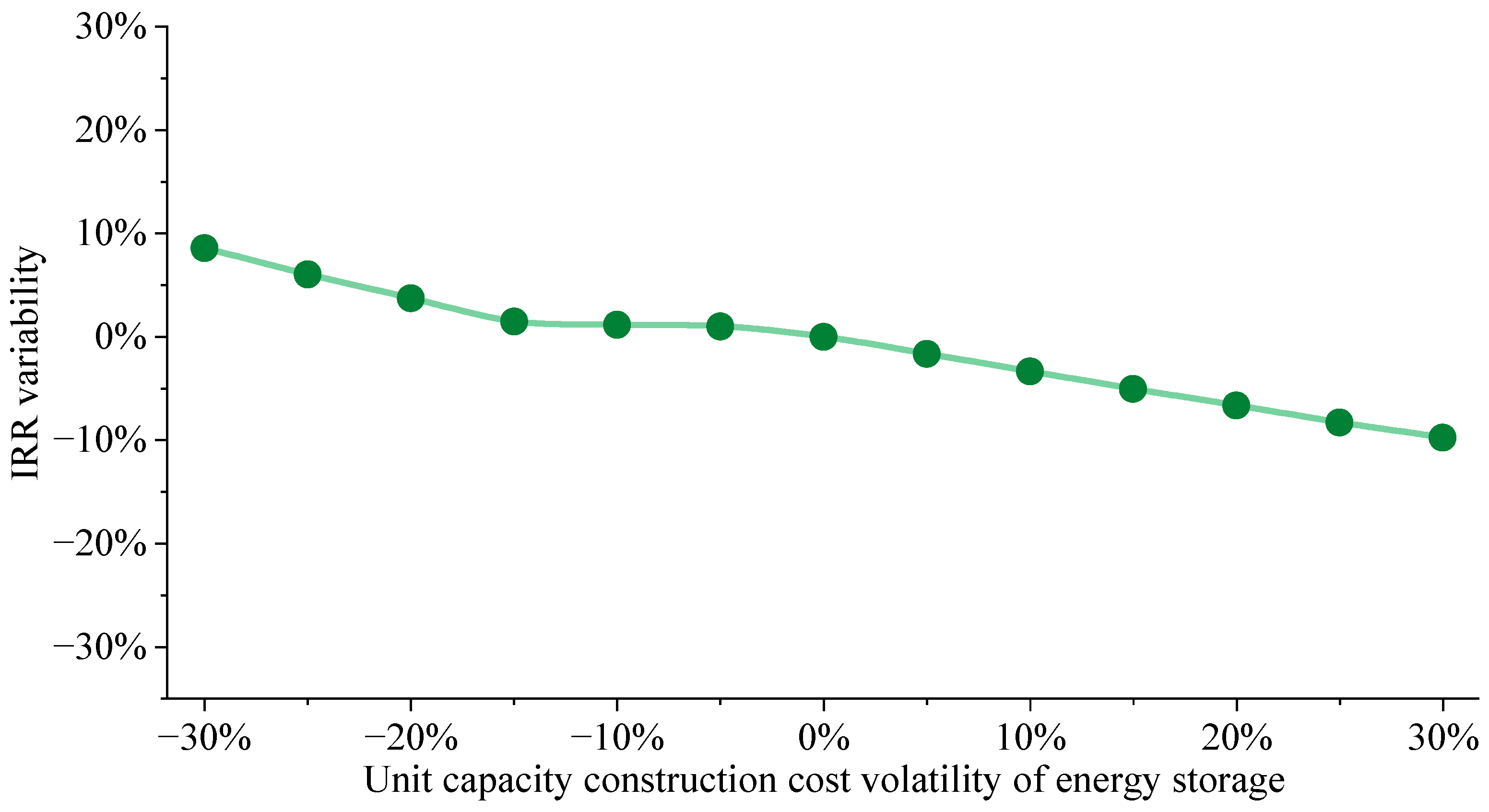
(3) Unit capacity construction cost volatility of energy storage

To evaluate the potential impact of volatility in the unit capacity construction cost of energy storage on the rural microgrid planning results, this subsection takes the simulated unit capacity construction cost (as shown in Table 2) as the benchmark, and analyzes the variations in the IRR of microgrid planning results under volatility of the benchmark unit capacity construction cost, as illustrated in Figure 13.

Figure 13. Changes in IRR under unit capacity construction cost volatility of energy storage.

As shown in Figure 13, the impact of energy storage cost volatility on the IRR ranges from −9.77% to +8.59%, showing an approximately symmetric negative correlation. It mainly affects the project economy through the investment stage while having a weak impact on the annual net profit (within ±3.5%). Furthermore, the sensitivity to market electricity price is significantly higher than that to energy storage cost, with the former being about three times that of the latter. This difference stems from the fact that electricity price directly affects the revenue side and has an operating leverage effect, whereas energy storage cost only affects the investment side and accounts for a limited proportion of the total cost. In summary, energy storage cost is a secondary factor; attention can be paid to the long-term downward trend brought by technological progress, and the short-term fluctuation risk is relatively controllable.

(4) Sensitivity Analysis of Shapley value weights

To evaluate the robustness of the Shapley value weighting method to volatility in objective function values, taking the benchmark values of the economic objective $F_1$ and the environmental objective $F_2$ as the center, $F_1$ and $F_2$ are independently fluctuated within the range of ±20%, respectively. The variation rules of the weights ${\mathsf{\omega }}_1$ and ${\mathsf{\omega }}_2$ are shown in Table 9.

Table 9. Sensitivity of Shapley value weights to objective function volatility.

${\mathit{F}}_1$ Volatility	${\mathit{F}}_2$ Volatility	${\mathit{\omega }}_1$ Volatility	${\mathit{\omega }}_2$ Volatility
0%	0%	-	-
10%	0%	3.85%	−4.17%
−10%	0%	−3.85%	4.17%
0%	10%	−3.85%	4.17%
0%	−10%	3.85%	−4.17%
20%	−10%	9.62%	−10.42%
−20%	10%	−9.62%	10.42%

As shown in Table 9, the weights exhibit a certain degree of robustness to volatility in objective functions. When a single objective fluctuates independently by ±10%, the variation amplitude of the weights is controlled within ±4%. This indicates that the Shapley value weighting method is insensitive to moderate objective estimation errors. Further analysis shows that the variation direction of the weights is consistent with expectations. When the economic objective $F_1$ increases, its marginal contribution to the comprehensive benefit rises, the weight ${\mathsf{\omega }}_1$ increases accordingly, and vice versa. This characteristic enables the weights to dynamically reflect changes in the relative importance between objectives. However, the weight adjustment is significant in scenarios with large fluctuation amplitudes. When $F_1$ increases by 20% and $F_2$ decreases by 10%, ${\mathsf{\omega }}_1$ rises 9.62% and ${\mathsf{\omega }}_2$ drops 10.42%. This indicates that when there is a large difference in objective values, the weights will tilt towards the dominant objective, reflecting the contribution-oriented allocation principle in cooperative games. In summary, the Shapley value weighting method has good robustness within a reasonable range of objective estimation errors, and its weights can dynamically reflect the game relationship between objectives, providing an objective and interpretable weighting mechanism for multi-objective decision-making.

5.6. Cross Regional Applicability and Direct Current Microgrid Expansion Feasibility Analysis

(1) Applicability analysis of cross regional

To evaluate the applicability of the method proposed in this paper under different regional conditions, this section conducts theoretical analysis and scenario deduction from two aspects: resource endowment and electricity price mechanism, which are shown in Table 10 and Table 11, respectively.

Table 10. Applicability under different resource endowments.

Resource Type	Typical Area	Impact on Model	Model Adaptability
Abundant wind and solar resources	Northwest China, Australian Outback	WT/PV output curves exhibit significant fluctuations, increasing the demand for energy storage	The model can automatically optimize energy storage capacity to smooth power output
General wind and solar resources	Central Europe, Eastern China	A larger installed capacity is required to meet the load	The model can achieve supply–demand balance through capacity optimization
Single resource dominance	Northern Europe (primarily wind power), Middle East (primarily solar power)	Simplifies the model by disabling a specific resource option	Model supports device type selection

Table 11. Applicability under different electricity market pricing mechanisms.

Electricity Market Pricing Mechanism	Typical Area	Impact on Model	Model Adaptability
Fixed electricity tariff	Germany	Predictable revenue and high certainty of optimization	The model can be directly applied to fixed electricity rates
Competitive bidding	China, Northern Europe	Fluctuations in electricity prices introduce revenue uncertainty	The model can be extended for stochastic optimization or scenario analysis
Net metering	United States, Australia	Excess electricity fed into the grid is sold at the same price as purchased electricity	The model requires adjustment to the payoff function, but the framework remains applicable

The proposed method shows good adaptability under different resource and electricity price environments, and its core advantages lie in configurable parameters, extensible modules, and reusable algorithms. For the practical application in specific regions, the localized migration of the method can be realized only by adjusting the input parameters and appropriately expanding the model modules. However, it still faces the following challenges:

Firstly, the initial investment scale of rural microgrids is relatively large, and social capital still faces obstacles such as limited financing channels and the lack of risk assessment mechanisms. It is feasible to explore a mixed investment model involving government guidance, social capital and village-level cooperatives, or introduce green financial tools to reduce financing costs.

Secondly, rural microgrids involve the coordination of multiple subjects including energy sources, power grids, loads, and energy storage. The current power system still has institutional obstacles in terms of grid-connection services, electricity price settlement, and dispatching authority. It is recommended to fully communicate with local power grid companies and energy authorities before the project is implemented to clarify the grid-connection process, electricity price policies, and benefit distribution mechanism.

Furthermore, the implementation effect of demand response is highly dependent on users’ willingness to participate. Some rural residents may be insensitive to electricity price signals or lack the motivation to actively adjust their electricity consumption behavior. We can improve user participation through publicity and guidance, demonstration leadership, profit sharing and other methods, and form a community of interests between microgrids and users.

(2) Feasibility analysis of direct current microgrid expansion

Direct current (DC) microgrids can connect DC sources and loads more efficiently, reduce losses in alternating current (AC)-DC conversion links, and improve system efficiency and reliability. They are particularly suitable for rural areas where the proportion of DC loads is increasing [36,37]. The core logic and solution framework of this paper are independent of the specific configuration of the power grid. Therefore, it is directly feasible in theory to apply this methodology to the research on capacity configuration and operation optimization of DC microgrids.

6. Conclusions

In this paper, a multi-objective optimization framework for rural microgrids considering both economic and environmental benefits is constructed. The positive environmental externalities are quantified as one of the optimization objectives, and the Shapley value method is introduced to realize cooperative game weighting among multiple objectives, overcoming the strong subjectivity limitation of the traditional weighting method. Furthermore, the global harmony search algorithm is adopted for solution, which significantly improves the computational efficiency while maintaining high convergence precision consistent with NSGA-II.

Under the optimal configuration scheme, the internal rate of return of the project reaches 23.04%, and the payback period is 5.32 years, which proves that the rural microgrid has sound economic feasibility and investment value. In addition, the rural microgrid can achieve an annual equivalent carbon emission reduction of 9.94 × 10⁴ tons, which provides a reproducible technical paradigm for the construction of a clean, efficient and reliable energy supply system in rural areas.

It is recommended to establish a differentiated electricity price mechanism and demand response incentive policies to guide users to actively participate in load regulation. Financial subsidies and grid-connection support for energy storage configuration should be increased to promote the large-scale promotion of the “wind–solar–storage integration” model. In addition, environmental benefits such as carbon emission reduction should be incorporated into the project evaluation system, and the transformation path from environmental value to economic benefits should be explored to enhance the sustainable operation capacity of rural microgrids.

In the future, we will expand a single rural microgrid to the collaborative planning of multi-microgrid clusters, and explore the interaction mechanism between rural energy systems and the higher-level power grid. Additionally, we will study the optimal configuration results of WT, PV and energy storage under the DC framework so as to quantitatively evaluate the comprehensive benefits of DC microgrids in rural areas.

References

- Shi, Z.; Liang, F.; Pezzuolo, A. Renewable energy communities in rural areas: A comprehensive overview of current development, challenges, and emerging trends. J. Clean. Prod. 2024, 484, 144336. [Google Scholar] [CrossRef] [Scilit]
- Li, J.; Liu, P.; Zhang, G.; Liu, H. Optimal planning and feasibility analysis of a grid-connected PV-biomass hybrid renewable energy system for rural electrification with electric vehicles: A case study of Hainan, China. Energy 2025, 324, 135986. [Google Scholar] [CrossRef] [Scilit]
- Song, D.; Chen, K.; Chen, R.; Fan, X.; Yang, J.; Dong, M.; Talaat, M.; Elkholy, M.H. A bi-level optimization approach for siting and sizing of distributed wind-storage power systems in rural areas based on MCTS and IPSO algorithms. Energy Convers. Manag. 2025, 342, 120173. [Google Scholar] [CrossRef] [Scilit]
- Zhu, T.; Chang, X.; Zhu, F.; Shen, Y.; Zhu, L.; Xu, C. Empirical study on sustainable energy development goals: Analysis of rural roof distributed photovoltaic systems in Jiangsu, China. Phys. Chem. Earth Parts A/B/C 2024, 136, 103711. [Google Scholar] [CrossRef] [Scilit]
- Guevara, M.; Manzini, F.; Sánchez-Juárez, A. Technical and economic analysis for the implementation of photovoltaic systems in agricultural zones of Mexico City: A case study. Energy Sustain. Dev. 2025, 87, 101743. [Google Scholar] [CrossRef] [Scilit]
- Koholé, Y.W.; Ngouleu, C.A.W.; Fohagui, F.C.V.; Tchuen, G. Quantitative techno-economic comparison of a photovoltaic/wind hybrid power system with different energy storage technologies for electrification of three remote areas in Cameroon using Cuckoo search algorithm. J. Energy Storage 2023, 68, 107783. [Google Scholar] [CrossRef] [Scilit]
- Chen, M.; Wei, J.; Yang, X.; Fu, Q.; Wang, Q.; Qiao, S. Multi-objective optimization of multi-energy complementary systems integrated biomass-solar-wind energy utilization in rural areas. Energy Convers. Manag. 2025, 323, 119241. [Google Scholar] [CrossRef] [Scilit]
- Tessemo, H.D.; Hassane, A.I.; Bikai, J.; Bot, B.V.; Lontsi, F.; Njock, P.J.; Sosso, O.T.; Mouangue, R.M. Techno-economic analysis of viability of two stand-alone water pumping systems for rural areas of Kanem oasis: Case studies of solar photovoltaic (PV) and solar organic Rankine cycle (ORC) systems. Results Eng. 2025, 25, 104391. [Google Scholar] [CrossRef] [Scilit]
- Sánchez-Lozano, D.; Aguado, R.; Escámez, A.; Awaafo, A.; Jurado, F.; Vera, D. Techno-economic assessment of a hybrid PV-assisted biomass gasification CCHP plant for electrification of a rural area in the Savannah region of Ghana. Appl. Energy 2025, 377, 124446. [Google Scholar] [CrossRef] [Scilit]
- Assouo, T.; Lontsi, F.; Boupda, O.; Koholé, Y.W.; Njitacke, Z.T. Modeling and techno-economic study of a hybrid renewable energy power plant for electrification in rural areas with an equatorial climate. Energy 2025, 320, 134983. [Google Scholar] [CrossRef] [Scilit]
- Rahimi, I.; Li, M.; Choon, J.; Pamuspusan, D.; Huang, Y.; He, B.; Cai, A.; Nikoo, M.R.; Gandomi, A.H. Optimizing renewable energy site selection in rural Australia: Clustering algorithms and energy potential analysis. Energy Convers. Manag. X 2025, 25, 100855. [Google Scholar] [CrossRef] [Scilit]
- Nwazor, N.O.; Aguni, J.N.; Okeke, R.O. Off-Grid Renewable Energy Solutions for Agro-Rural Community Development in Nigeria. Adv. Sci. Technol. 2025, 160, 195–204. [Google Scholar]
- Li, Y.; Liu, C.; Wang, Y.; Xiao, T.; Liu, J.; Li, Y. Benefit comprehensive evaluation for pumped storage power station boosting rural revitalization in the surrounding areas in China. Renew. Energy 2025, 238, 121895. [Google Scholar] [CrossRef] [Scilit]
- Zhou, Y.; Wang, J.; Gao, W.; Han, G. Multi-temporal-spatial collaboration for multiperiodic management of distributed energy system with cloud storage, productivity and renewables sharing. J. Energy Storage 2025, 132, 117736. [Google Scholar] [CrossRef] [Scilit]
- Gbadega, P.A.; Sun, Y.; Balogun, O.A. A Unified Optimization Framework for Cost-Effective and Voltage-Stable Operation of Renewable Energy-Based Microgrids Using Mixed-Integer Nonlinear Programming. e-Prime-Adv. Electr. Eng. Electron. Energy 2025, 12, 101010. [Google Scholar] [CrossRef] [Scilit]
- Coady, J.; Duquette, J. Quantifying the impacts of biomass driven combined heat and power grids in northern rural and remote communities. Renew. Sustain. Energy Rev. 2021, 148, 111296. [Google Scholar] [CrossRef] [Scilit]
- Liu, M.; Liao, M.; Wang, P.; Li, C.; Zhao, X. Multi-timescale power self-balancing optimization and regulation of remote rural microgrids based on stochastic monte carlo method. J. Phys. Conf. Ser. 2025, 2960, 012014. [Google Scholar] [CrossRef] [Scilit]
- Roldán-Blay, C.; Escrivá-Escrivá, G.; Roldán-Porta, C.; Dasí-Crespo, D. Optimal sizing and design of renewable power plants in rural microgrids using multi-objective particle swarm optimization and branch and bound methods. Energy 2023, 284, 129318. [Google Scholar] [CrossRef] [Scilit]
- Li, H.; Li, P.; Yue, X.; Zheng, Y.; Zu, W.; Zhang, H. A study on the optimal allocation of photovoltaic storage capacity for rural new energy microgrids based on double-layer multi-objective collaborative decision-making. Sustain. Energy Res. 2025, 12, 1. [Google Scholar] [CrossRef] [Scilit]
- Zhao, G.; Zhang, C.; Ren, Q. A Two-Layer Optimal Scheduling Strategy for Rural Microgrids Accounting for Flexible Loads. Energy Eng. 2024, 121, 3355. [Google Scholar] [CrossRef] [Scilit]
- Güven, A.F.; Yörükeren, N.; Samy, M.M. Design optimization of a stand-alone green energy system of university campus based on Jaya-Harmony Search and Ant Colony Optimization algorithms approaches. Energy 2022, 253, 124089. [Google Scholar] [CrossRef] [Scilit]
- Qian, J.; Sun, X.; Zhong, X.; Zeng, J.; Xu, F.; Zhou, T.; Shi, K.; Li, Q. Multi-objective optimization design of the wind-to-heat system blades based on the Particle Swarm Optimization algorithm. Appl. Energy 2024, 355, 122186. [Google Scholar] [CrossRef] [Scilit]
- Heroual, S.; Belabbas, B.; Allaoui, T.; Denai, M. Performance enhancement of a hybrid energy storage systems using meta-heuristic optimization algorithms: Genetic algorithms, ant colony optimization, and grey wolf optimization. J. Energy Storage 2024, 103, 114451. [Google Scholar] [CrossRef] [Scilit]
- Sun, X.; He, H.; Ma, L. Harmony search meta-heuristic algorithm based on the optimal sizing of wind-battery hybrid micro-grid power system with different battery technologies. J. Energy Storage 2024, 75, 109582. [Google Scholar] [CrossRef] [Scilit]
- Huang, Y.; Sun, Q.; Zhang, N.; Wang, R. A multi-slack bus model for bi-directional energy flow analysis of integrated power-gas systems. CSEE J. Power Energy Syst. 2021, 10, 2186–2196. [Google Scholar]
- Ren, F.; Cao, X. Optimal operation of integrated energy system with carbon capture and demand response. Appl. Therm. Eng. 2025, 280, 128216. [Google Scholar] [CrossRef] [Scilit]
- Chen, X.; Zhan, M. A necessary and sufficient condition for weighted Shapley values in the core. Econ. Lett. 2025, 256, 112618. [Google Scholar] [CrossRef] [Scilit]
- Kong, F.; Zhang, D.; Song, M.; Zhou, X.; Wang, Y. Collaborative scheduling and benefit allocation for waste-to-energy, hydrogen storage, and power-to-gas under uncertainties with temporal relevance. Energy 2024, 307, 132650. [Google Scholar] [CrossRef] [Scilit]
- Jing, W.; Aksoy, M.; Rahman, M.A.; Alenezi, A.H.; Deriche, M.; Tao, H. Multi-objective planning and optimal configuration of wind, solar, and energy storage in interconnected microgrid clusters using Vine Copula scenario generation and antlion optimization. Renew. Energy 2025, 256, 124313. [Google Scholar] [CrossRef] [Scilit]
- Wang, Y.; Song, M.; Jia, M.; Li, B.; Fei, H.; Zhang, Y.; Wang, X. Multi-objective distributionally robust optimization for hydrogen-involved total renewable energy CCHP planning under source-load uncertainties. Appl. Energy 2023, 342, 121212. [Google Scholar] [CrossRef] [Scilit]
- Wang, Y.; Song, M.; Jia, M.; Shi, L.; Li, B. TimeGAN based distributionally robust optimization for biomass-photovoltaic-hydrogen scheduling under source-load-market uncertainties. Energy 2023, 284, 128589. [Google Scholar] [CrossRef] [Scilit]
- Wang, J.; Qiu, R.; Wang, Z.; Xi, G. Low carbon economic dispatch of electric-hydrogen-blended natural gas integrated energy system with multi-energy coupling and integrated demand response. Energy 2025, 344, 139769. [Google Scholar] [CrossRef] [Scilit]
- Wang, H.; Yuan, L.; Wang, W.; Song, M. Distributionally robust optimization for pumped storage power station capacity expanding based on underwater hydrogen storage introduction. Energy 2024, 310, 133254. [Google Scholar] [CrossRef] [Scilit]
- Li, Y.; Song, M.; Hu, Y.; Wang, Y.; Han, Y.; Li, B.; Zhang, F. Fishery Microgrid Planning Involving Surface Photovoltaic and Hydrogen/Oxygen Utilization under Typical Extreme Scenarios. Renew. Energy 2026, 261, 125292. [Google Scholar] [CrossRef] [Scilit]
- Hu, J.; Ji, X.; Wang, H.; Feng, G.; Song, M. Hydrogen-Involved Renewable Energy Base Planning in Desert and Gobi Regions Under Electricity-Carbon-Hydrogen Markets. Processes 2025, 13, 3655. [Google Scholar] [CrossRef] [Scilit]
- Doostinia, M.; Beheshti, M.T.H.; Alavi, S.A.; Guerrero, J.M. Distributed event-triggered average consensus control strategy with fractional-order local controllers for DC microgrids. Electr. Power Syst. Res. 2022, 207, 107791. [Google Scholar] [CrossRef] [Scilit]
- Doostinia, M.; Beheshti, M.T.H.; Alavi, S.A.; Guerrero, J.M. Distributed control strategy for DC microgrids based on average consensus and fractional-order local controllers. IET Smart Grid 2021, 4, 549–560. [Google Scholar] [CrossRef] [Scilit]
Disclaimer/Publisher’s Note: The statements, opinions and data contained in all publications are solely those of the individual author(s) and contributor(s) and not of MDPI and/or the editor(s). MDPI and/or the editor(s) disclaim responsibility for any injury to people or property resulting from any ideas, methods, instructions or products referred to in the content. |
© 2026 by the authors. Licensee MDPI, Basel, Switzerland. This article is an open access article distributed under the terms and conditions of the Creative Commons Attribution (CC BY) license.