


Abstract
Gross Domestic Product (GDP) serves as a core indicator for measuring the sustainable economic development of countries and regions. Accurate understanding of its spatio-temporal distribution is crucial for achieving the United Nations Sustainable Development Goals (SDGs). However, current grid-based GDP data for China’s regions predominantly consists of data from specific years, making it difficult to capture fine-grained changes in economic development. To address this, this study proposes a spatial GDP framework integrating cross-scale feature extraction (CSFs) with stacked ensemble learning. Based on China’s county-level GDP statistics and multi-source auxiliary data, it first generates a density-weighted estimation layer. This is then processed through dasymetric mapping to produce China’s Annual High-Resolution Gridded GDP Dataset (CA_GDP) from 2000 to 2021. Evaluation demonstrates the framework’s superior performance in density weight estimation, achieving an R2 of 0.82 against statistical data. Compared to traditional single models like Random Forests (RF), it improves R2 by 13–54%, reduces mean absolute error (MAE) by 2–26%, and lowers root mean square error (RMSE) by 19–39%, with these advantages remaining stable across time series. The dasymetric mapping of the CA_GDP dataset clearly depicts the economic development patterns and urban agglomeration effects in the southeastern coastal regions, as well as the relatively lagging economic development in western areas. Compared to existing public datasets, CA_GDP offers significant advantages in reflecting the fine-grained economic spatial structure within county-level units, providing a more reliable data foundation for identifying regional economic disparities, policy formulation and evaluation, and related research.
1. Introduction
Gross Domestic Product (GDP) is one of the most commonly used macroeconomic indicators for measuring economic development levels and regional economic patternsADDIN. It is widely applied in various fields, including macro-level planning, poverty identification, disaster risk assessment, and resource allocation, making it crucial for policy formulation and regional sustainable development [1,2,3]. However, traditional GDP estimation methods primarily rely on government departments that aggregate data based on administrative units [4]. This approach has several drawbacks, such as data updating delays, difficulties in data collection, and an inability to reveal economic distribution disparities within administrative units [5]. Additionally, it often struggles to integrate with gridded environmental variables [6,7,8], which limits its application in various contexts. To more accurately reflect the economic distribution differences within administrative units, converting traditional statistical data into gridded GDP data is of significant importance [9].
In the field of gridded GDP data research, scholars have made continuous efforts to advance the evolution of gridding methods. Specifically, traditional regression models, which characterized linear relationships in the early stages [9,10,11], gradually evolved into quadratic polynomial [9,12,13] and exponential models [14,15] capable of capturing nonlinear features. In recent years, machine learning models, such as Random Forest (RF) [16,17,18,19], Gradient Boosting [20,21], and Neural Networks [22], have become mainstream. Concurrently, the auxiliary data systems have become more diverse, expanding from the initial reliance on a single source, such as nighttime light data (NTL) [12,23], to integrating multi-source remote sensing data, including land use, population distribution, and NDVI [20,22,24]. This expansion allows for a more comprehensive depiction of the spatial patterns of economic activities. During this process, spatial resolution has also made significant strides, with high-resolution grids not only enhancing spatial accuracy but also providing deeper insights into the micro-level characteristics of economic heterogeneity [22,25]. However, current feature extraction methods, which model economic data by averaging remote sensing variables within administrative units, have failed to effectively reflect economic distribution and spatial heterogeneity within these units, limiting the ability to identify micro-scale economic activities [26,27,28]. The Cross-Scale Feature Extraction (CSFs) method [27] addresses this issue by replacing the administrative unit averages with finer-grained group-level values. This reduces the scale mismatch between administrative units and pixels, increases the number and range of training samples, and alleviates scale discrepancy issues [29]. Additionally, individual machine learning methods often have inherent drawbacks, such as instability, insufficient generalization ability, and inefficiency in capturing extreme values [30,31,32]. Stacked ensemble learning, by combining predictions from multiple models during the training process, significantly improves the stability and robustness of predictions [33,34] and has achieved remarkable results in related fields [34,35,36,37]. Therefore, the combination of CSFs and stacked ensemble learning allows for the effective integration of the high spatial heterogeneity advantage of the former with the multi-model stacking advantage of the latter, reducing cross-scale differences and enabling the accurate transfer of feature information.
As the world’s second-largest economy, China’s rapid economic growth has been accompanied by significant spatiotemporal heterogeneity [38]. Analyzing the complex regional economic distribution patterns within China is not only key to understanding its economic miracle but also holds great importance for enriching and advancing the theory of spatial economics. Existing studies based on single-point data [22,24] have overcome the limitations of administrative boundaries, but they struggle to reveal the dynamic processes and underlying mechanisms that shape these patterns. Therefore, there is an urgent need to create a long-term gridded GDP dataset to gain deeper insights into the spatiotemporal evolution of China’s regional economy.
In this study, we construct a GDP spatialization framework that combines the CSFs method with stacked ensemble learning to generate China’s Annual High-Resolution Gridded GDP Dataset (CA_GDP) from 2000 to 2021. We compare the GDP weight results predicted by the stacked model with those from traditional single models, such asRF, to validate the model’s effectiveness. Furthermore, through dasymetric mapping, we calibrate the county-level statistical totals to grid cells, resulting in the corrected CA_GDP. Finally, we visually compare CA_GDP with other publicly available datasets to verify the reliability of our dataset.
2. Data and Methods
2.1. Data
The datasets used in this study include two categories (excluding Hong Kong, Macau, and Taiwan). The first category is the county-level GDP statistical data. The second category consists of gridded covariate data, including population data, NLT, electricity consumption, annual mean temperature, Normalized Difference Vegetation Index (NDVI), Net Primary Production (NPP), land cover data, and Digital Elevation Model (DEM) data.
2.1.1. County-Level GDP Statistical Data
The county-level GDP statistical data for 2000 to 2021 used in this study are sourced from the China Regional Economic Statistical Yearbook, China Urban Statistical Yearbook, China County Statistical Yearbook, and various provincial statistical yearbooks. Due to anomalies in GDP data for some county-level administrative units and changes in administrative boundaries, data for certain regions are missing. In terms of time, some years for certain regions have missing data. Considering the spatial autocorrelation of economic distribution (Table S1), this study uses the product of the annual growth rate of the nearest neighbor administrative unit and the GDP of the previous year to impute missing values. A total of 2367 county-level units’ GDP data from 2000 to 2021 were collected. Finally, the county-level GDP statistical data from 2000 to 2021 were linked to the corresponding administrative units.
2.1.2. Gridded Covariate Data
In GDP downscaling studies, it is often necessary to integrate multi-source auxiliary data to reduce the uncertainty caused by spatial heterogeneity, thereby improving the accuracy of converting traditional statistical GDP to gridded GDP. Remote sensing data, with its high resolution, low cost, and ability to quickly capture large-scale surface features, has become an advanced technology widely used to reflect the latest social and economic information [1]. Therefore, remote sensing data is frequently used as auxiliary data in GDP downscaling [39]. Based on previous research [16,24,25,40,41], this study selects the following auxiliary variables:
Population density is a core indicator for measuring the intensity of regional economic activity. Areas with high population density, particularly urban regions, are often associated with higher production efficiency and consumption demand, making them strong indicators for GDP [3,42]. The population density data for 2000–2020 and 2021 used in this study come from the WorldPop and Global Gridded Population (GlobPOP) datasets, which have been widely used in urban planning, environmental simulation, and regional economic measurement [8,43,44].
NTL data is widely used as a proxy for regional economic activity, especially in areas lacking traditional economic data. The NTL data used in this study are from the DMSP-OLS-like dataset, constructed by Zheng et al. [45]. This dataset combines monthly DMSP-OLS and SNPP-VIIRS data, providing a continuous light series for China from 1992 to 2022. The dataset has been widely validated for its effectiveness in GDP estimation, urban expansion monitoring, and regional imbalance studies.
Land cover types reveal the economic structure and land use patterns of a region and are indispensable variables in spatial economic analysis. The land cover data used in this study comes from the annual China Land Cover Dataset (CLCD) [46], which classifies land cover into 9 categories using RF. To meet the modeling requirements, the 30 m resolution grid data were aggregated to a 1000 m resolution, and the spatial density of each land cover type was calculated to characterize the spatial patterns of different land cover types.
Electricity consumption data can, to some extent, indicate the level of industrialization and economic activity in a region [47]. (Given the lack of electricity consumption data for 2020 and 2021, the model training still uses data from 2019.) Temperature and DEM data represent the potential impacts of climate and geographical environment on the spatial distribution of economic activities [48]. Additionally, the NDVI and NPP are important variables for measuring natural resources and ecological vitality, which are closely related to the agricultural economy and ecosystem services [49,50].
The detailed descriptions of the data sources are displayed in Table 1.
Table 1.
Overview of the datasets used in this study.
Due to the differences in resolution and coordinate systems among the various gridded datasets, we converted all grid datasets to the Albers Equal-Area projection (central meridian 105° E, standard parallels 25° N/47° E) and applied a China region mask. Simultaneously, bilinear interpolation was used to resample the grid data to a 1 km resolution. All data processing was implemented using the ArcGIS 10.8 platform and Python 3.8-related libraries.
2.2. Methods
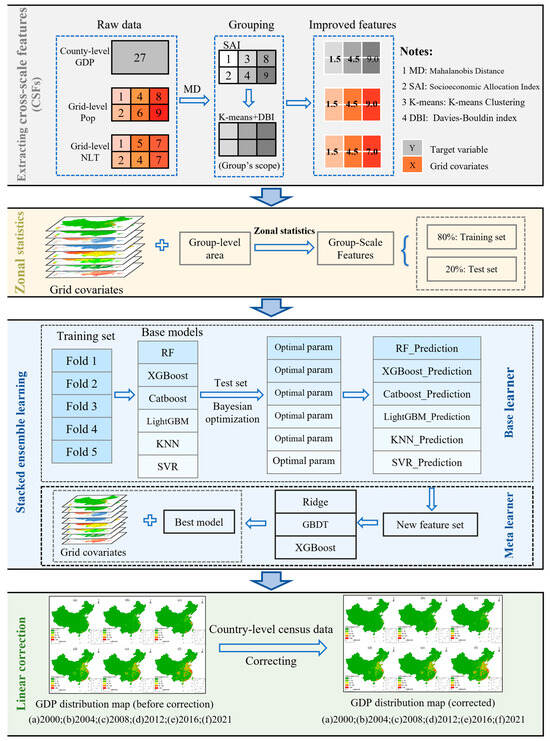
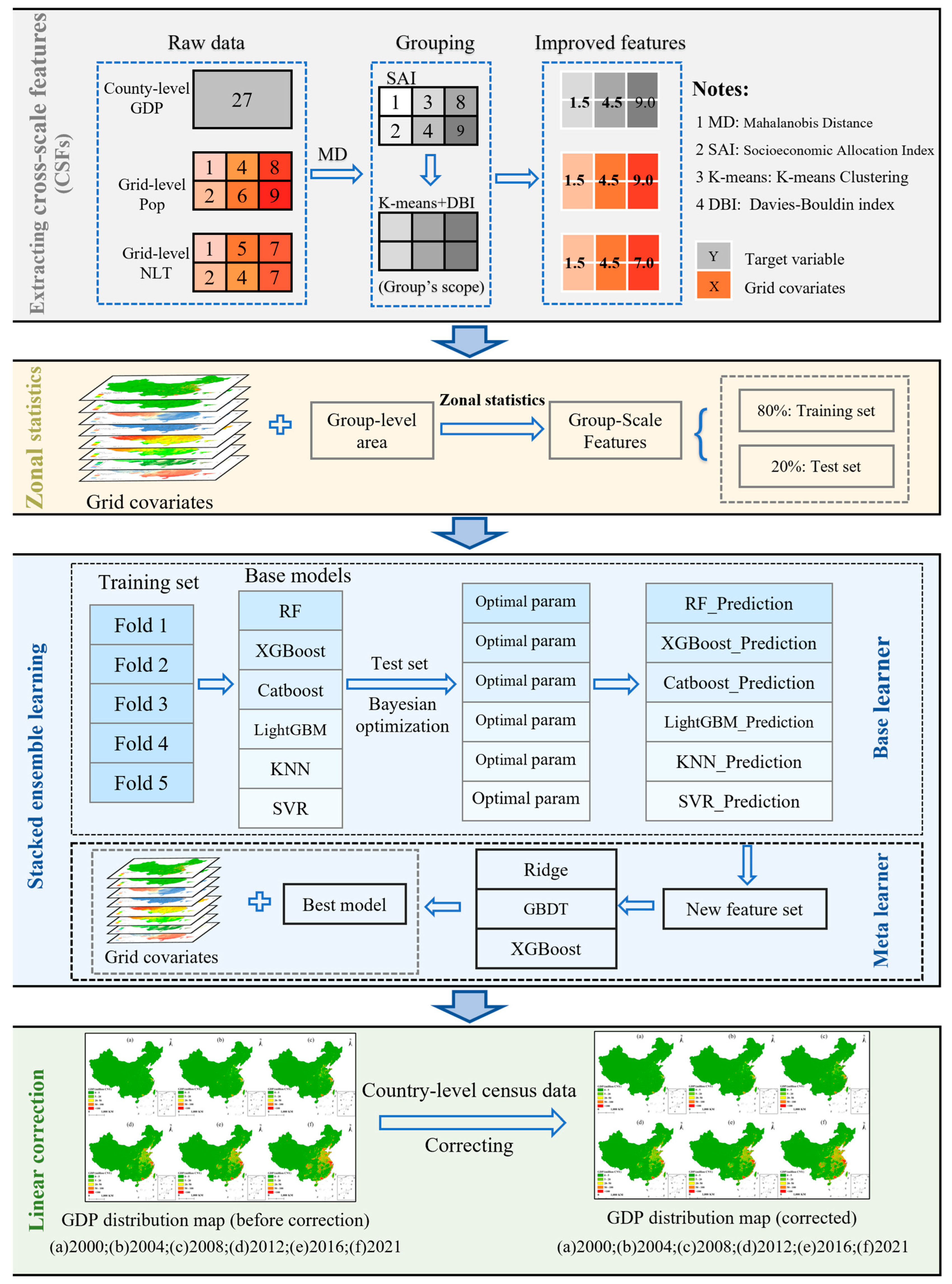
This study employs a method combining the CSFs with stacked ensemble learning. By extracting more refined and representative features and integrating the advantages of multiple base models, the method captures surface spatial distribution and economic activity patterns, thereby improving the accuracy and stability of the model. Finally, by performing linear calibration of the predicted GDP grid data with county-level statistical data, a high-precision GDP gridded dataset for 2000 to 2021 was constructed (Figure 1).
Figure 1.
GDP spatialization flowchart.
2.2.1. Improved Cross-Scale Feature Extraction Method
In traditional methods, auxiliary variables at the grid scale are often spatially aggregated within administrative units, typically using the mean value of the administrative region as a feature for model training. However, this region-based statistical approach neglects the spatial heterogeneity within the administrative unit, which can lead to information loss and, consequently, systematic overestimation or underestimation biases in spatial predictions. To address this issue, this study employs the CSFs method.
First, the Socioeconomic Allocation Index (SAI) is used to initially downscale the county-level GDP data. This is achieved by spatially distributing the data at the pixel scale based on Formula (1). SAI is constructed using population density and NTL data to form a feature vector, and its composite weight is calculated using Mahalanobis distance, as detailed in Formula (2). Next, K-means clustering [51] is applied to the preliminary pixel-level GDP data for grouping, with K ∈ [2, 5]. To determine the optimal number of clusters, the Davies–Bouldin Index (DBI) is introduced as a clustering evaluation metric, as shown in Formula (4). A smaller DBI value indicates higher intra-group compactness and greater inter-group separability, thus better reflecting a reasonable internal structure. Finally, by combining the results of the previous two steps, the clustering boundaries within each county are determined, and the mean values of all independent and dependent variables within each group are calculated. This process refines the spatial granularity from county-level averages to group-level averages, providing approximate real training samples for high-resolution modeling without the need for external training labels.
where and represent the GDP value of pixel and the census statistics value of county , respectively. denotes the SAI of pixel , while represents the sum of the SAI of all pixels within county .
where is the SAI of pixel , is the feature vector matrix of pixel , is the mean of all valid pixels, and is the covariance matrix.
where represents the DBI coefficient when the number of clusters is ; and are the average distances between groups and , respectively. and are the distances from the centers of groups and , respectively.
2.2.2. GDP Spatialization Model Based on Stacked Ensemble Learning
Given the limitations of single models in capturing the complex nonlinear relationships between GDP and its multi-source driving variables, this study introduces a Stacking Ensemble Learning strategy [52] to improve modeling accuracy [53]. A stacked ensemble framework was implemented to integrate multiple base learners for robust GDP estimation. Six algorithms—RF [54], Extreme Gradient Boosting (XGBoost) [55], Categorical Boosting (CatBoost) [56], Light Gradient Boosting Machine (LightGBM) [57], K-Nearest Neighbors (KNN) [58], and Support Vector Regression (SVR) [59]—served as diverse base learners. Each was tuned via Bayesian Optimization, maximizing the 5-fold cross-validated R2 to prevent overfitting and ensure generalization. In this process, the data were split into five folds; each iteration used four folds for training and one for validation, with final performance averaged across all folds. Once tuned, the base models were retrained on the full dataset. Their out-of-fold predictions from cross-validation were concatenated into a new feature matrix, which was used to train candidate meta-learners (Ridge Regression (Ridge) [60], Gradient Boosting Decision Tree (GBDT), and XGBoost). The meta-learner with the highest validation R2 was selected to synthesize the base models’ predictions, yielding the final gridded GDP weight estimate. (The optimal parameter settings for the model are provided in Tables S2–S7.)
2.2.3. Accuracy Evaluation Method
To validate the effectiveness and reliability of the proposed method, we compare the model’s predicted values with the census statistics values to evaluate its performance in spatial estimation. Statistical indicators such as the coefficient of determination (R2), Root Mean Square Error (RMSE), and Mean Absolute Error (MAE) are used to assess the model’s fitting accuracy and generalization ability from multiple dimensions, including correlation, consistency, and error magnitude. This ensures the efficiency and reliability of the model in reconstructing the spatial distribution of GDP.
where and represent the census GDP value and predicted GDP value for county , respectively. is the average of the census data for all counties, and is the sample size.
2.2.4. Dasymetric Mapping
After completing the initial spatialization predictions and considering the inevitability of model fitting errors, this study further introduces a linear correction method based on county-level statistical values to adjust the pixel-level GDP values output by the model, ensuring that the total GDP at the county scale is consistent with the official data. The specific correction formula is as follows:
where represents the corrected GDP for the grid cell, denotes the predicted GDP for the grid cell before correction, is the statistical GDP value of county , and is the predicted GDP value of county .
For counties with missing statistical data, a spatial calibration method based on the pixel proximity principle is applied. Specifically, the calibration coefficient of a missing pixel is assigned as that of the nearest spatially adjacent pixel that has already been calibrated.
3. Results
3.1. Accuracy Evaluation Results
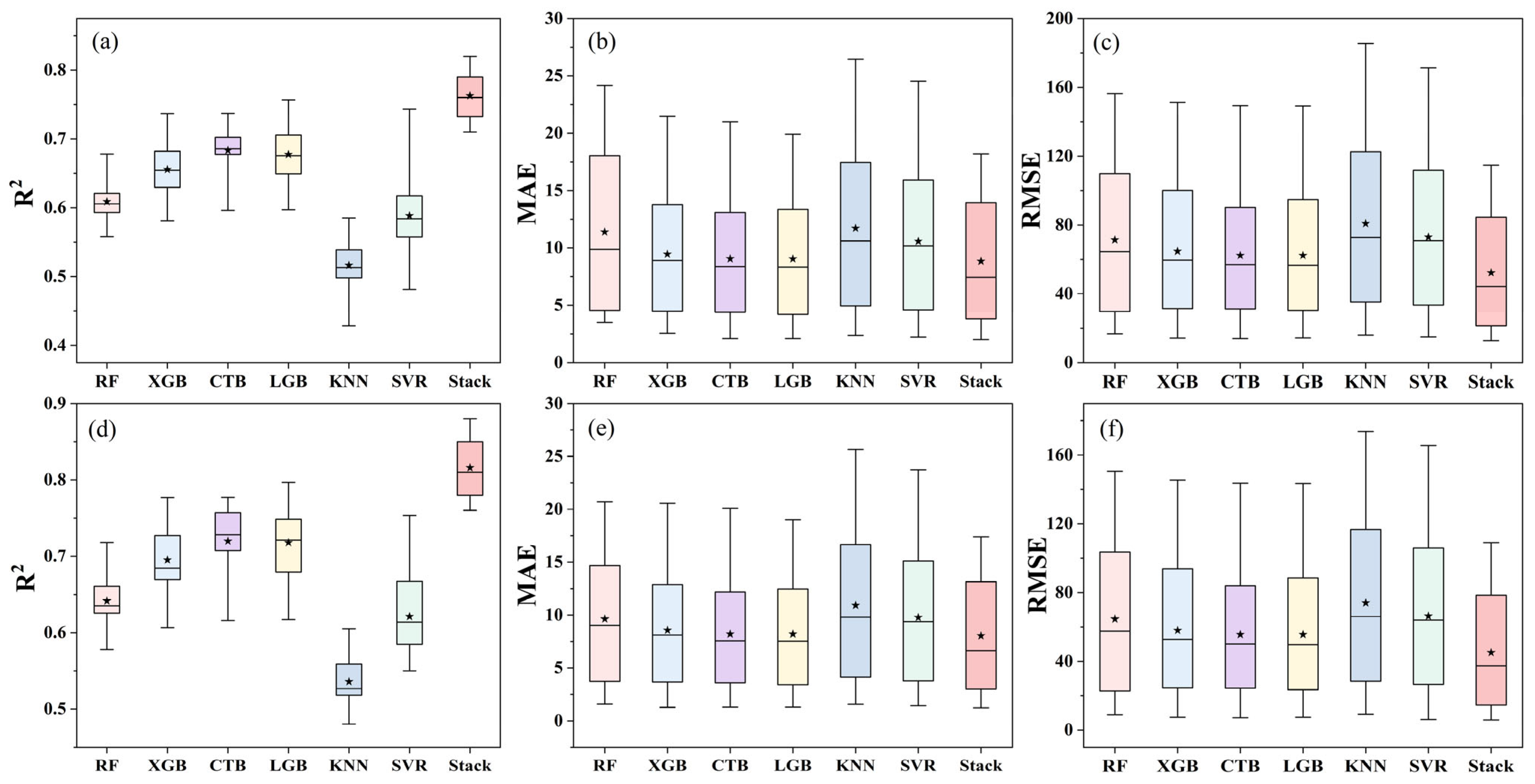
Since county-level scale is currently the finest level of GDP statistics in China, to assess the reliability of the GDP weighting simulation, this section will aggregate the simulated weights (before dasymetric mapping) at the county level and compare them with county-level statistical data for verification. The CSFs and stacked ensemble model achieved the best performance in all metrics for the results before dasymetric mapping. The average R2 reached 0.82, which is 7% higher than the stacked ensemble model without CSFs (R2 = 0.76) and 13–54% higher than other single models like RF (R2 = 0.53–0.72). In terms of error, the MAE before dasymetric mapping was 8.04, lower than the Stack model without CSFs (8.83) and the single models (9.45–11.71 million CNY·km−2). The RMSE was 45.12, lower than the stacked ensemble model without CSFs (52.23) and the single models (55.61–74.01 million CNY·km−2). The error was the lowest among all models. The stacked ensemble model outperformed other models in accuracy, consistency, and error control, thereby fully validating the applicability and advancement of the method proposed in this study for high-resolution, long-term GDP gridding (Figure 2).
Figure 2.
Box plots of evaluation metrics for each model from 2000 to 2021: (★): mean; (a–c) represent the evaluation metrics without using CSFs; (d–f) represent the evaluation metrics after using CSFs. Here, RF refers to Random Forest, XGB refers to Extreme Gradient Boosting, CTB refers to Categorical Boosting, LGB refers to Light Gradient Boosting Machine, KNN refers to K-Nearest Neighbors, SVR refers to Support Vector Regression, and stacked refers to the stacked ensemble model.
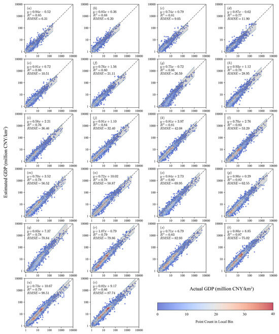
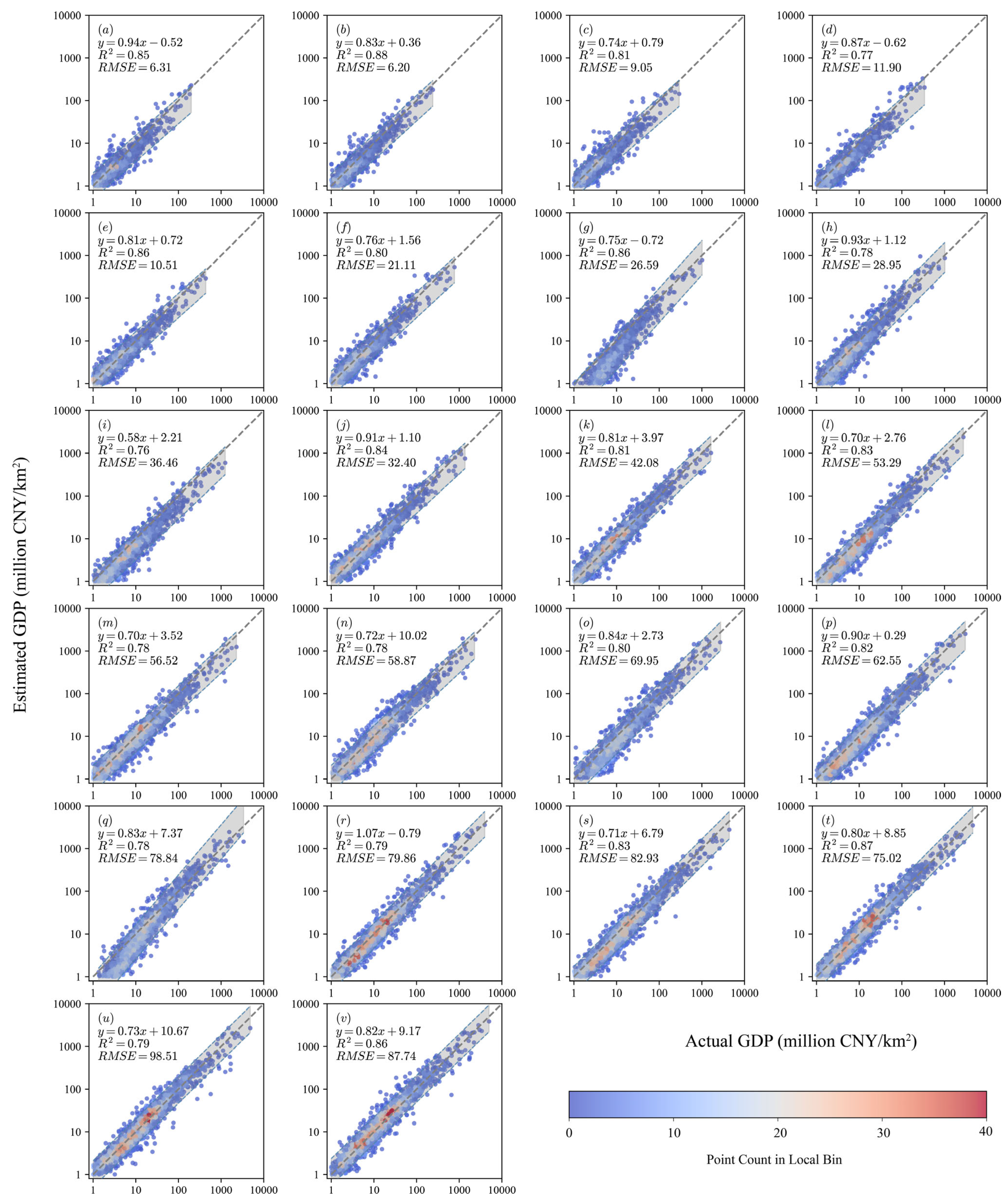
The comparison between the actual county-level GDP and GDP weights is shown in Figure 3. Overall, R2 remains between 0.76 and 0.88, indicating the strong fitting ability of the model across different years. As actual GDP continuously increases, the RMSE rises from about 6.31 in 2000 to 87.74 in 2021 (million CNY·km−2), while the MAE increases from 2.4 to 19.11 (million CNY·km−2), reflecting the effect of scaling on absolute error, while the relative accuracy remains stable. The regression slope is generally less than 1, revealing slight underestimation in high GDP regions and slight overestimation in low-value intervals. Overall, the model demonstrates robustness across multiple orders of magnitude and long time series, accurately capturing the spatial patterns and evolutionary trends of GDP intensity at the county level in China.
Figure 3.
Evaluation results of actual GDP weight and estimated GDP weight for Chinese counties from 2000 to 2021. (a)2000 (b) 2001; (c) 2002; (d) 2003; (e) 2004; (f) 2005; (g) 2006; (h) 2007; (i) 2008; (j) 2009; (k) 2010; (l) 2011; (m) 2012; (n) 2013; (o) 2014; (p) 2015; (q) 2016; (r)2017; (s) 2018; (t) 2019; (u) 2020; (v) 2021.
3.2. Comparison of National Annual GDP Statistics and Predicted Data
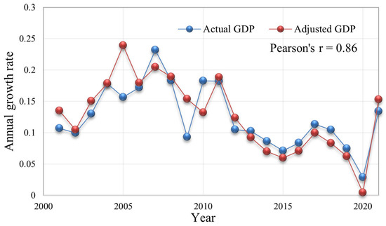
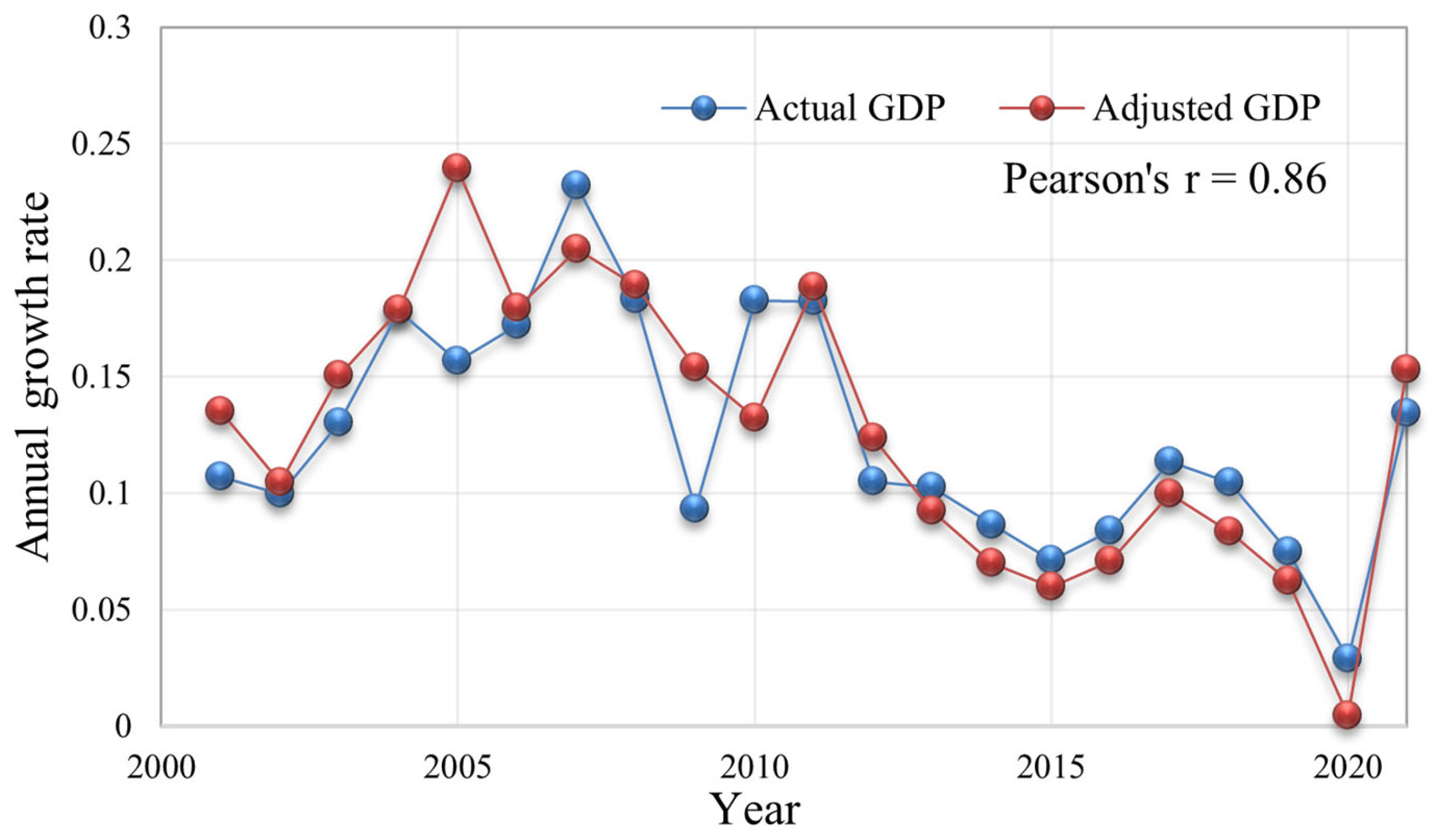
After calibrating the county-level statistical totals to grid cells through dasymetric mapping, the final CA_GDP data were obtained, and all subsequent analyses are based on this dataset. The results of the linear fitting between the aggregated CA_GDP pixel values and the national annual GDP total (Figure S3) show that the Pearson correlation coefficient for the GDP levels from 2000 to 2021 is as high as 0.998, validating the consistency in aggregate levels. Furthermore, to address potential autocorrelation in the time series and to evaluate the model’s capacity to capture economic dynamics, we compared the annual growth rates derived from the aggregated CA_GDP and the statistical data. The two growth rate series exhibit a strong correlation (Pearson’s r = 0.86, Figure 4), indicating that our model effectively replicates the year-to-year changes in China’s economic growth over the study period.
Figure 4.
Comparison of annual GDP statistics and estimated annual growth rates in China from 2000 to 2021.
3.3. Long-Term Time Series GDP Gridded Maps
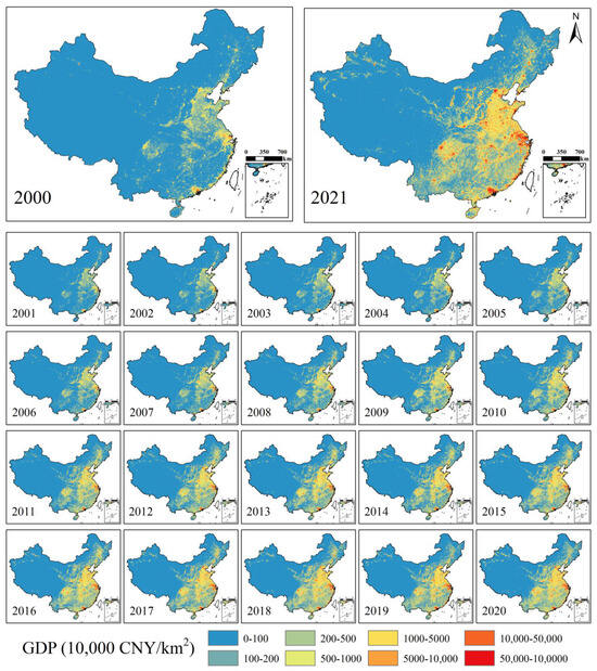
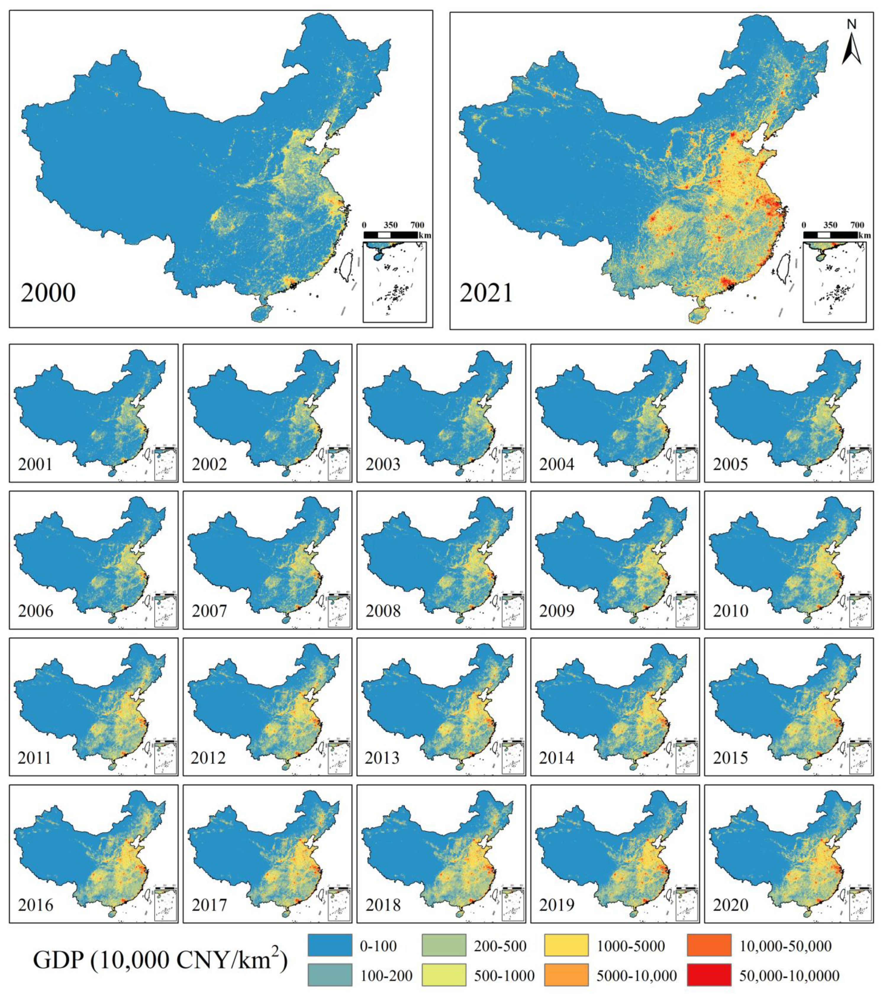
From the GDP gridded data of 2000–2021 (The GDP distribution chart for the intermediate years is provided in Figure S1), it is evident that China’s economy has experienced rapid growth (Figure 5). From the perspective of spatial changes, the distribution of GDP in China from 2000 to 2021 shows a significant pattern of high-value regions, such as provincial capitals, acting as growth poles, with continuous diffusion into the surrounding areas. The spatial connections between neighboring growth poles have become increasingly closer, and the continuity of economic activities has steadily strengthened. Notably, in regions such as the Yangtze River Delta, Pearl River Delta, and Beijing–Tianjin–Hebei, high-density economic zones of contiguous development have emerged [61].
Figure 5.
Gridded GDP estimates for China’s mainland regions from 2000 to 2021 after linear correction.
In terms of spatial distribution patterns, a hierarchical urban cluster system has formed nationwide, driven by multiple core cities. This system includes the following regional clusters: the Yangtze River Delta, the Pearl River Delta, the Beijing–Tianjin–Hebei region, the Chengdu–Chongqing area, the Bohai Bay region, the Central Plains urban cluster, the Central and Southern region (Wuhan–Changsha–Nanchang), and Fujian (Fuzhou–Quanzhou–Xiamen). This is attributable to the “Priority Eastern Development” strategy launched at the end of the 20th century and the evolving industrial landscape: large-scale infrastructure investments have driven the expansion and integration of major urban clusters, manufacturing has shifted from coastal hubs to inland regions, and high-end productive services have clustered in first-tier cities. Meanwhile, the economic development in the western regions lags. China still faces issues such as unequal and inadequate economic development, and there is a continued need to promote high-quality growth.
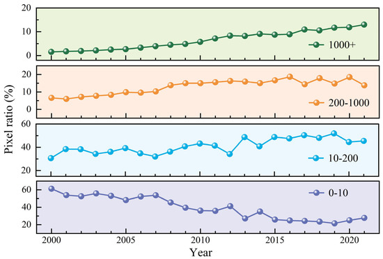
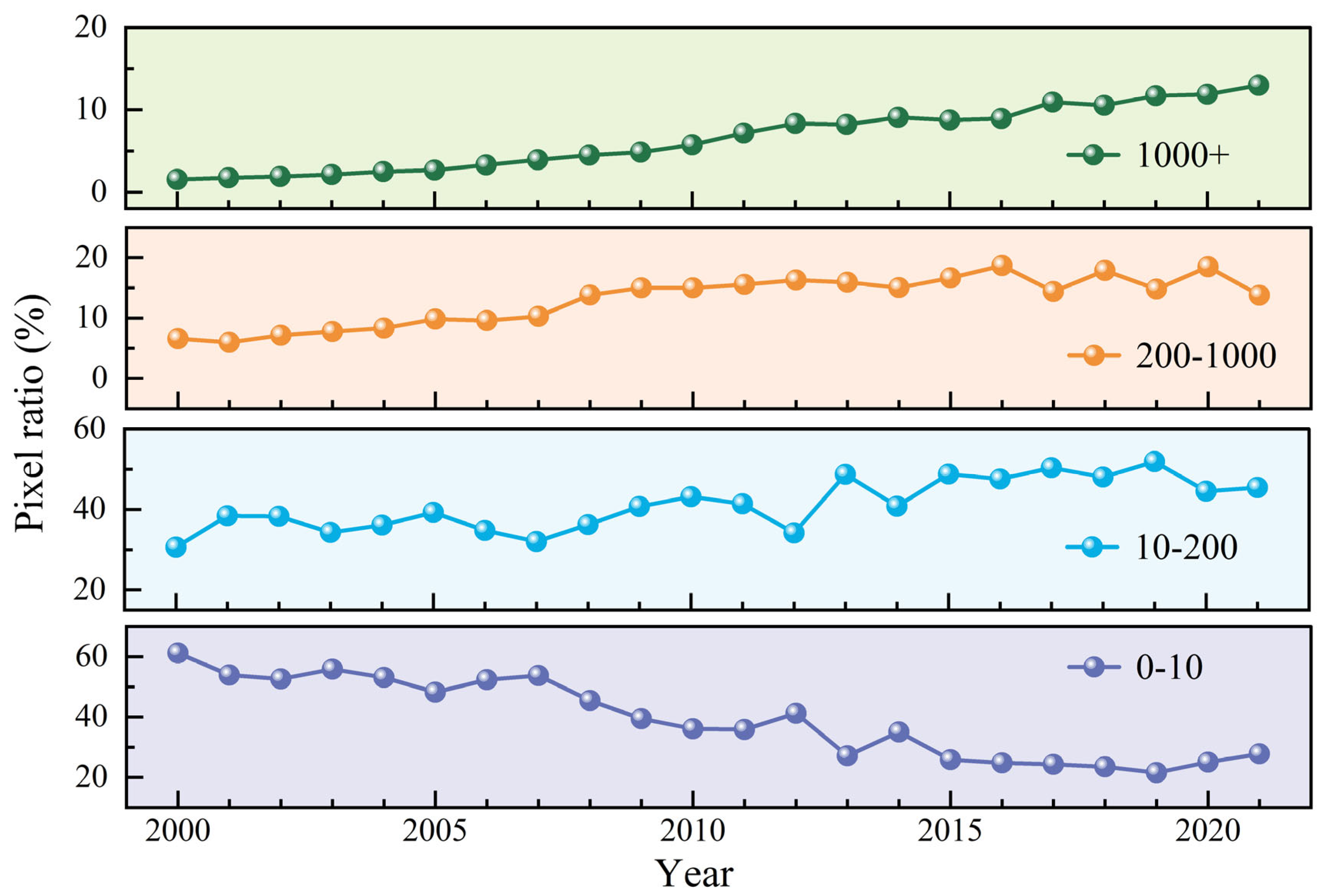
To more intuitively analyze the changing trend of income disparity between 2000 and 2021, this study divides the GDP values into four intervals: low (0–10 CNY), low-middle (10–200 CNY), middle-high (200–1000 CNY), and high (>1000 CNY), and systematically analyzes the relationship between the grid proportions of each interval and the time changes (Figure 6). This analysis helps reveal the spatial evolution of regions with different economic levels and their dynamic changes in the overall economic distribution, providing visualized data support for a deeper understanding of China’s economic inequality and its spatiotemporal evolution. From 2000 to 2021, China’s economic development underwent significant changes, with noticeable shifts in the pixel proportions of different GDP intervals. From 2000 to 2010, the proportion of low-value regions rapidly decreased, while the proportion of middle-high and high-value regions significantly increased (among which, in 2003, due to the SARS epidemic, the proportion of low-value regions experienced a brief increase [62]). Between 2010 and 2015, some low-value areas saw their GDP rise to the low-middle range. From 2015 to 2020, economic growth continued, but the growth rate of middle-high value regions slowed. Between 2020 and 2021, due to the widespread impact of the COVID-19 pandemic on China’s economy [63], some regions experienced a decline in GDP.
Figure 6.
Proportions of grid cells in each value interval of the CA_GDP data (10,000 CNY/km2).
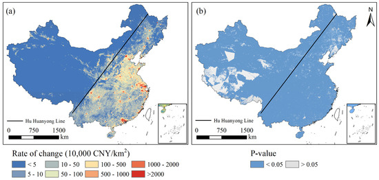
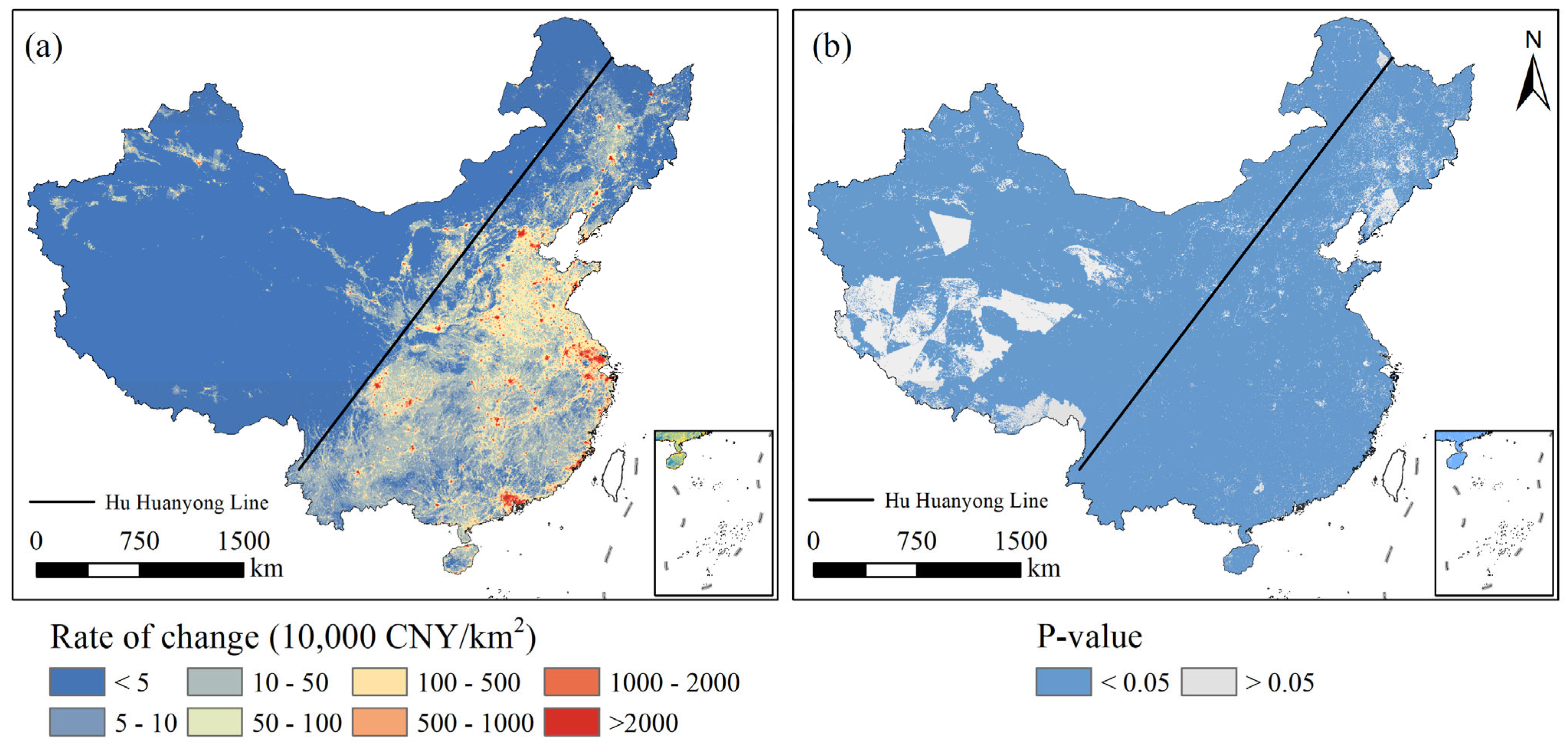
Based on pixel-level linear regression analysis, this study further obtains the regression coefficients and p values for each pixel from 2000 to 2021 (Figure 7). The regression coefficients represent the annual average growth rate of GDP, while the p values are used to assess the significance of the trend (with p < 0.05 indicating significance). The results show that high-value areas of economic growth are primarily located east of the Hu Line [64], especially in the Yangtze River Delta, Pearl River Delta, and Beijing–Tianjin–Hebei urban agglomerations, where the growth trend is most prominent. In contrast, economic growth in regions west of the Hu Line is relatively slow. From the spatial distribution of p values, the economic growth trend is significant in most areas of the country. However, constrained by geographical conditions and a resource-based industrial structure, growth trends in Tibet Autonomous Region and parts of Northeast China have been relatively slower.
Figure 7.
Distribution of regression coefficients (a) and p-values from 2000 to 2021 (b).
4. Discussion
4.1. Comparison with Publicly Available Gridded GDP Datasets
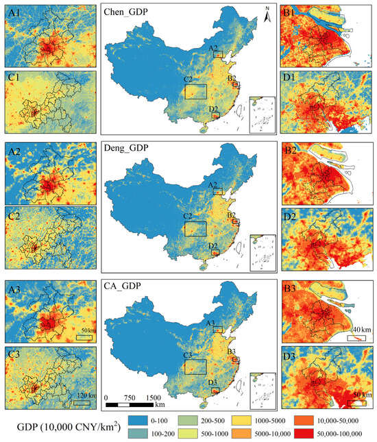
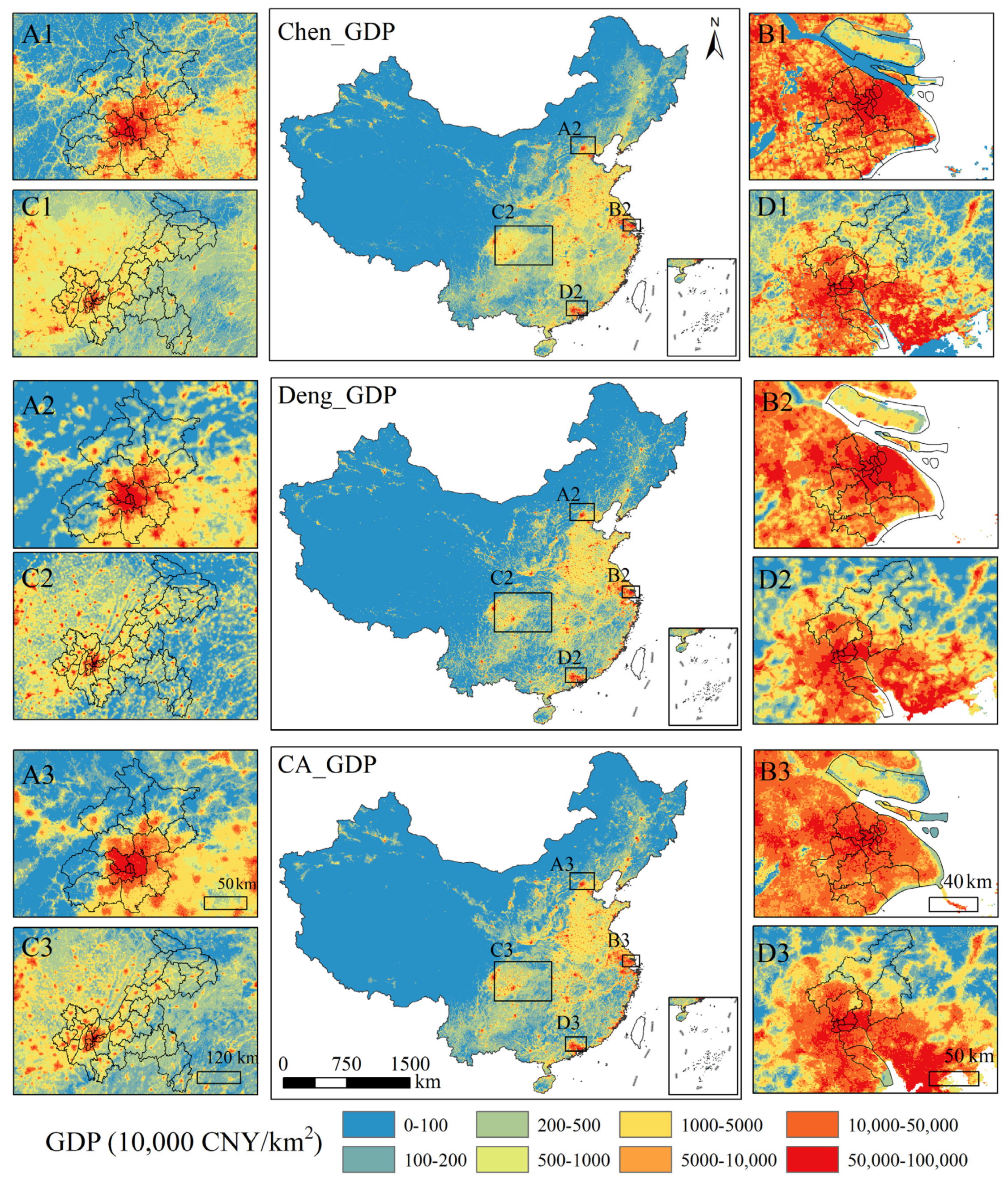
In this study, the GDP weight for 22 years was predicted and compared with county-level statistical values, achieving an average R2 of 0.82. Previous studies have shown that when R2 exceeds 0.7, the spatial characteristics of GDP are well described, which partially validates the feasibility of our GDP spatialization method and results. Building on this, we compared the CA_GDP dataset with the 2019 GDP gridded data from Chen_GDP [22] and Deng_GDP [24] (Figure 8). Our model’s R2 of this method reaches 0.82, which is higher than Chen et al.’s 0.72 [22] and Deng et al.’s 0.78 [24]. From the perspective of GDP spatial distribution, China’s economic distribution shows a typical “strong east, weak west” pattern, with economic activity being highly concentrated in coastal developed regions, while economic development in inland areas, particularly in the western regions, remains relatively lagging. In terms of the comparison in locally magnified regions, the CA_GDP is highly consistent with the other two datasets in terms of economic distribution patterns. In contrast, our dataset offers finer temporal resolution, surpassing both the annual data from Chen_GDP and the five-year intervals of Deng_GDP.
Figure 8.
Comparison of Chen_GDP, Deng_GDP, and CA_GDP datasets: (A1–A3) Beijing; (B1–B3) Shanghai; (C1–C3) Chongqing; (D1–D3) Guangzhou.
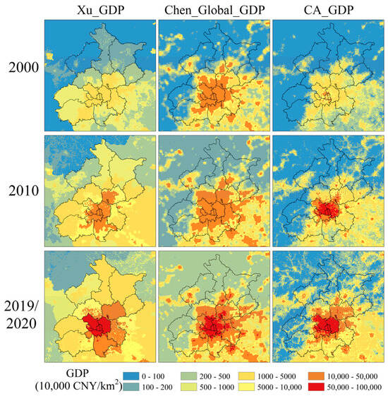
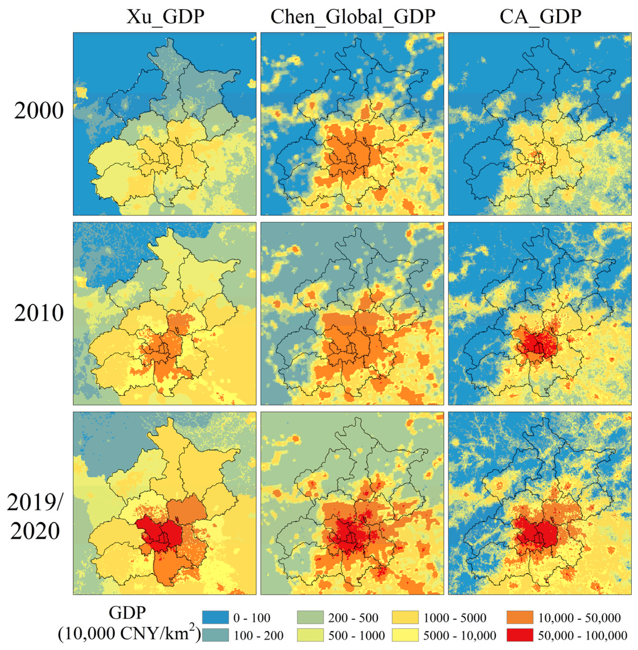
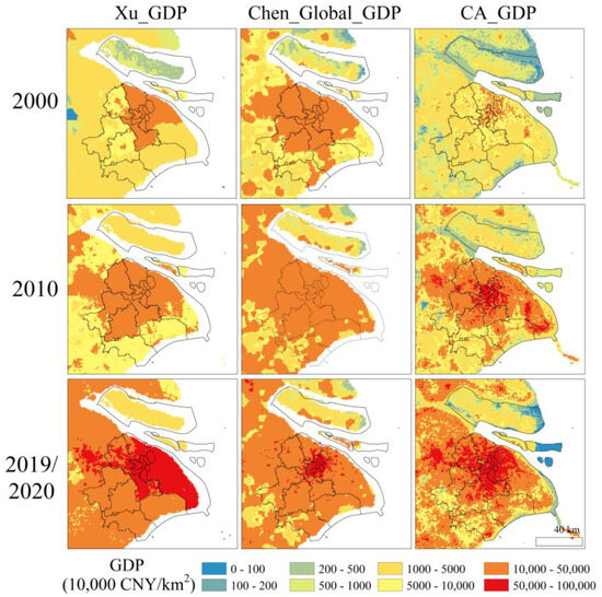
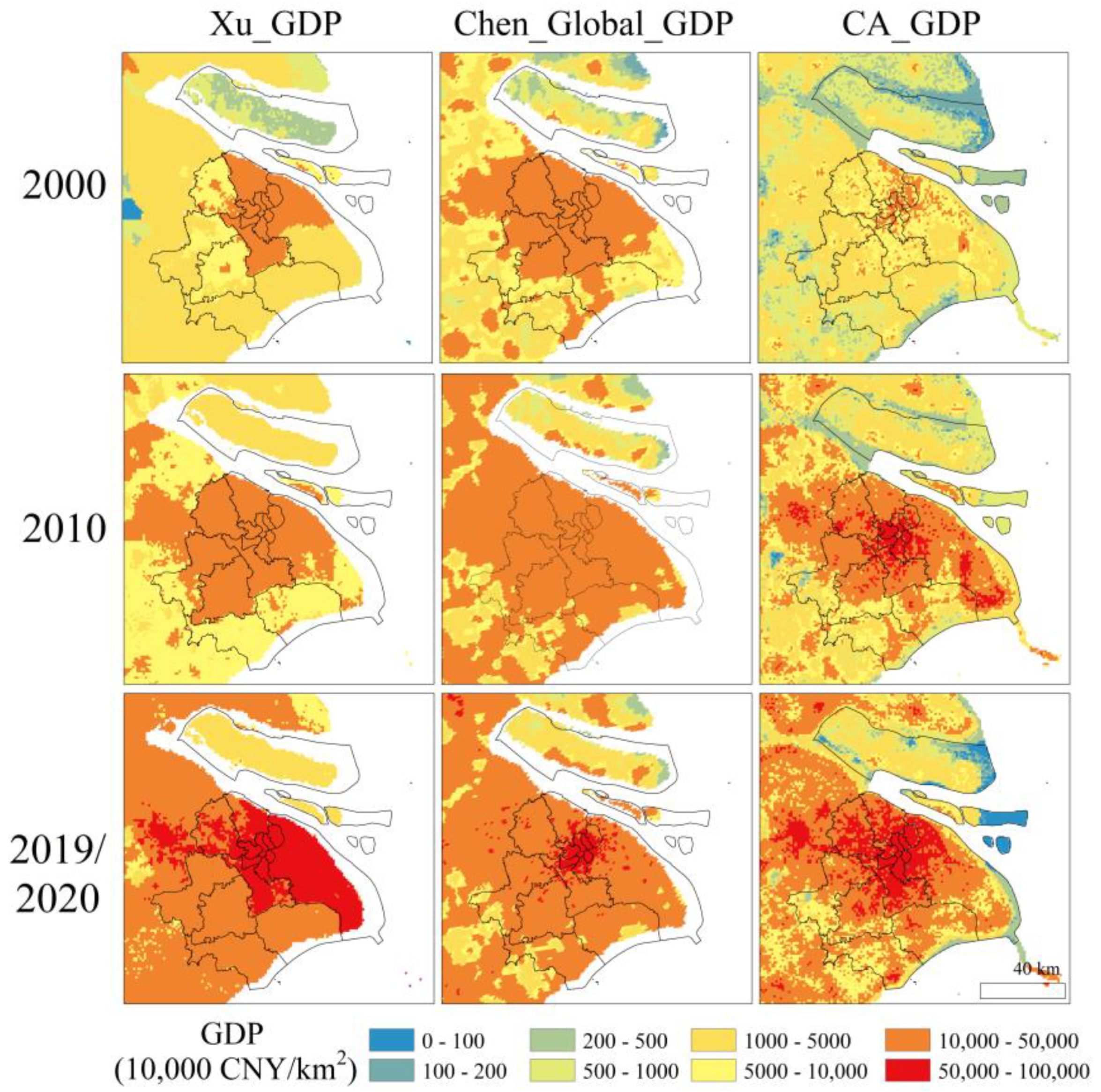
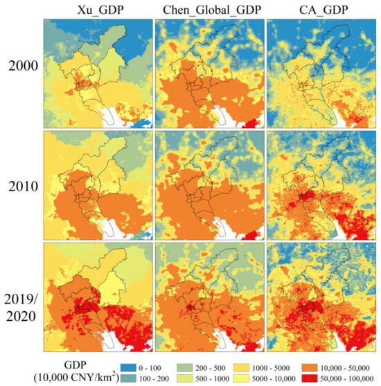
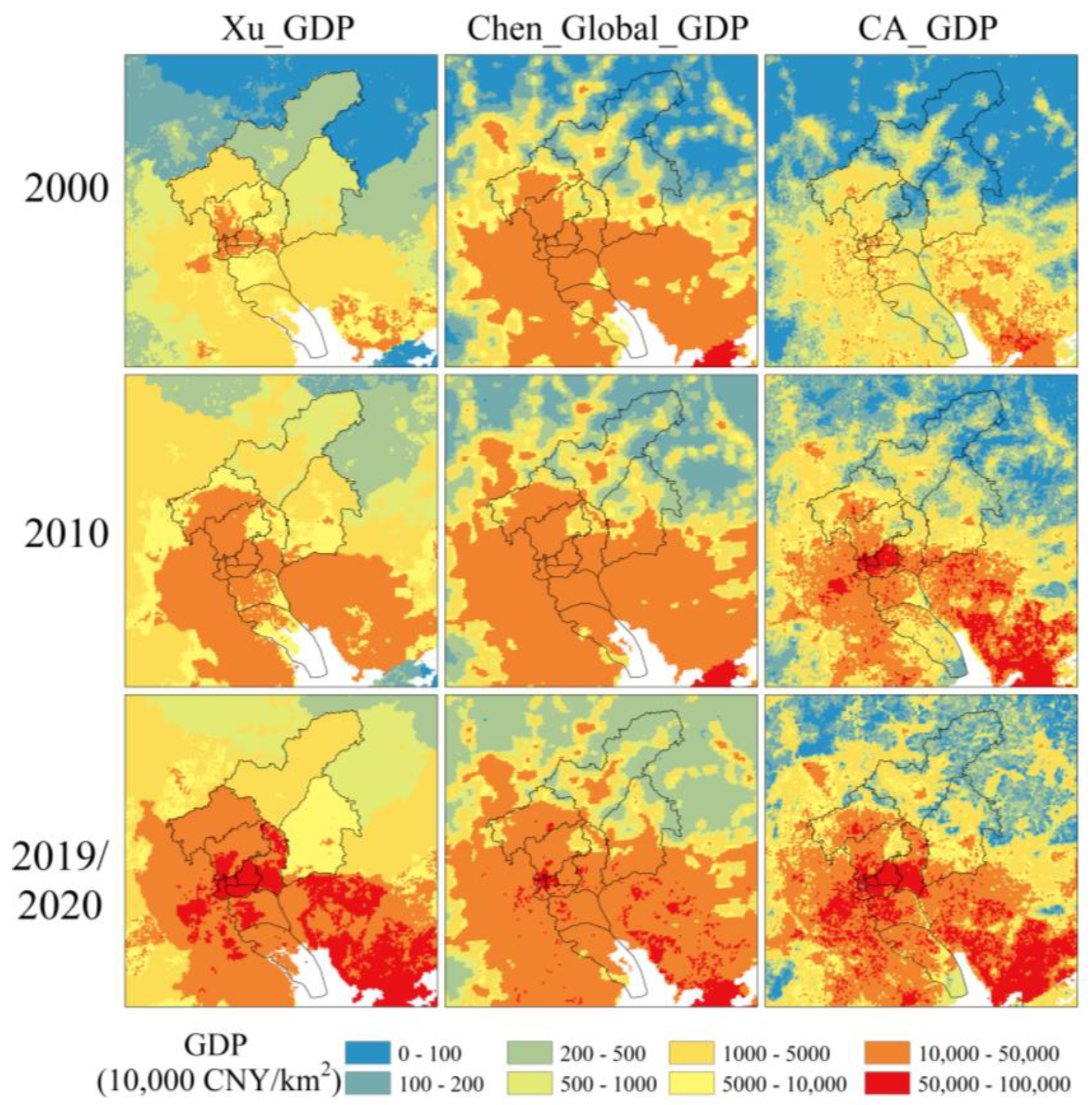
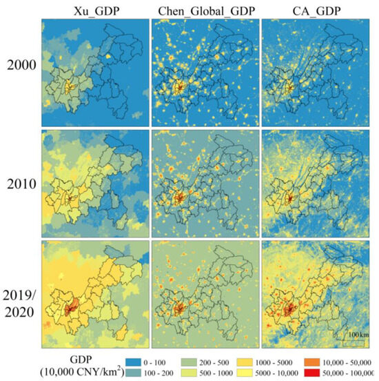
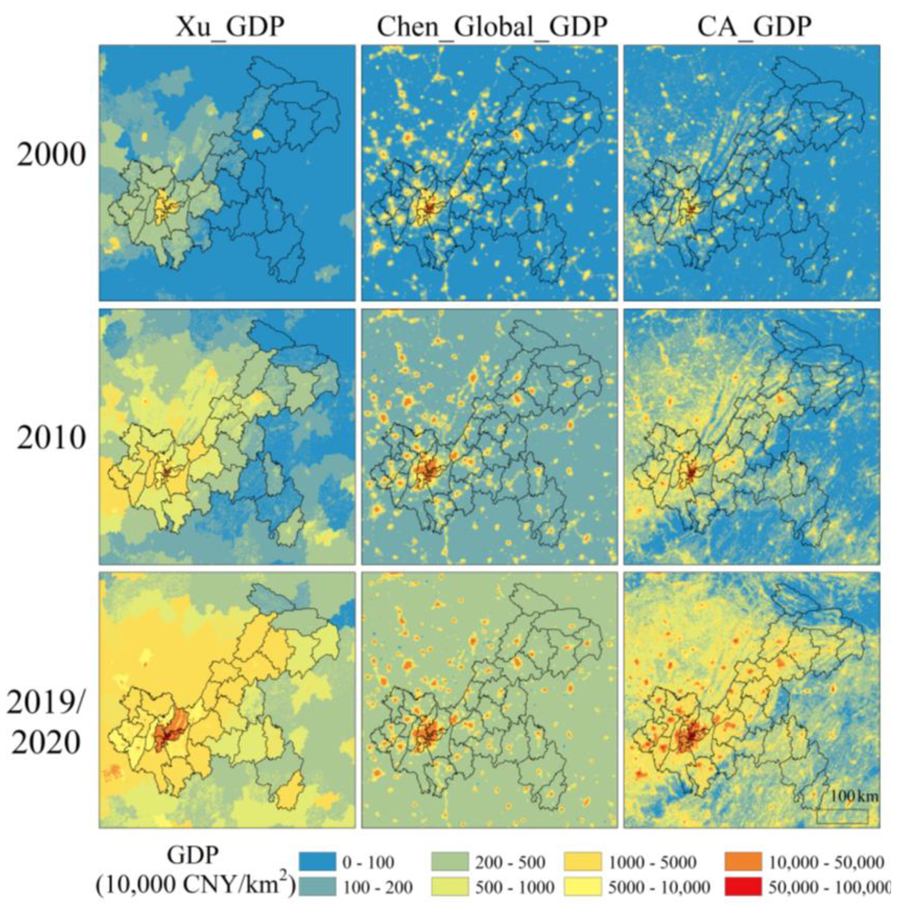
Furthermore, since the Chen_GDP and Deng_GDP datasets only provide data for a single year, they cannot reflect the long-term evolution of economic distribution. We further compared the publicly available datasets for 2000, 2010, and 2020 (i.e., Xu_GDP [65], Chen_Global_GDP [47]) with CA_GDP and performed spatial analysis on representative cities (Beijing, Shanghai, Guangzhou, and Chongqing) (Figure 9, Figure 10, Figure 11 and Figure 12). Since the Chen_Global_GDP dataset lacks data for 2020, we used the 2019 data as a substitute. The three datasets exhibit similar trends in spatiotemporal evolution, with economic activity in city core areas continuing to grow and gradually expanding to surrounding regions. The difference lies in the distribution: Xu_GDP data is relatively uniform within county-level administrative units, with noticeable boundary effects; Chen_Global_GDP data shows significant overestimation in non-urban areas (Figure S2); whereas CA_GDP provides a more detailed depiction of economic distribution within administrative units and avoids overestimation in non-urban areas. From a temporal perspective, all three datasets show rapid economic growth and the expansion of high-value regions, while CA_GDP is able to more accurately reflect the expansion trends of economic clusters over time, closely aligning with China’s actual economic development policies and regional coordination strategies [61].
Figure 9.
Comparison of GDP gridded datasets for Beijing.
Figure 10.
Comparison of GDP gridded datasets for Shanghai.
Figure 11.
Comparison of GDP gridded datasets for Guangzhou.
Figure 12.
Comparison of GDP gridded datasets for Chongqing.
4.2. Advancement of the Method
The innovation and advancement of this study lie in the use of a framework combining CSFs and stacked ensemble learning, which effectively overcomes issues such as insufficient accuracy and weak generalization ability in traditional high-resolution GDP spatialization modeling. The R2 of this method reaches 0.82, which is higher than Chen_GDP (0.72) [22] and Deng_GDP (0.78) [24]. The average MAE is 8.0 (million CNY·km−2), lower than Chen_GDP (24.1 (million CNY·km−2)) and Deng_GDP ( 8.6 (million CNY·km−2)). This method significantly improves the accuracy of GDP spatialization and effectively reduces errors, validating its accuracy and stability. This performance improvement is primarily due to the synergistic effect of CSFs and stacked ensemble learning. The CSFs method converts the traditional over 2000 county-level effective features into more than 6000 fine-grained group-level features, effectively mitigating the scale mismatch between administrative units and pixels, and thereby more accurately depicting the spatial heterogeneity of economic activities. Stacked ensemble learning, on the other hand, combines the advantages of multiple base learners, reducing the instability and bias of single models, and showing stronger robustness in fitting complex nonlinear relationships [33,34]. As a result, the high-resolution GDP gridded data generated by this study not only reveals the internal differences in regional economies more accurately but also offers superior stability, making it highly valuable for long-term dynamic analysis and prediction in complex scenarios. It provides a more reliable tool for decision support in related fields.
4.3. Limitations and Future Work
The method of this study performed well in improving the spatial accuracy and stability of GDP, but there are still two main limitations in data and model application. First, at the data level, the study mainly relies on county-level statistical GDP data and multi-source remote sensing data. Although it covers economic activities from 2000 to 2021, the county-level data is outdated or has missing errors [66]. In particular, the remote sensing data in small cities and rural areas has low resolution, which makes it difficult to accurately reflect local economic activities and affects the accuracy of the model and the accuracy of the prediction. It is recommended to be rigorous when analyzing economic errors on highly precise spatial scales. Second, at the model level, although CSFs and stacked ensemble learning methods are used to improve accuracy, in high-GDP areas, due to the small number of samples, the model training process focuses too much on the features of low-GDP areas, resulting in a large prediction error in high-GDP areas and affecting the universality of the model.
To address these limitations, the following strategies are proposed to enhance future gridded GDP datasets. First, integrating higher-resolution imagery (e.g., Sentinel-2, Landsat-9) [67,68] with geospatial big data like mobile signaling, POI density, and road networks [20,24,40,69] can improve spatial granularity in rural regions, capturing fine-grained activity where statistical coverage is weak. Second, to reduce errors in high-GDP areas, techniques such as sample re-weighting [70] or imbalance-aware algorithms [71] can be adopted to better model economic hotspots. Furthermore, independently modeling the three GDP sectors—agriculture, industry, and services—using sector-specific variables [20,24] would allow deeper analysis of industrial spatial distribution. Finally, incorporating time series models could help forecast gridded GDP dynamics, mitigating data lag and supporting forward-looking policy and planning.
5. Conclusions
This study constructed a CA_GDP dataset spanning 2000 to 2021, aiming to balance precision and stability in long-term GDP grid-based data modeling. Its core methodology innovatively combines Critical Success Factors (CSFs) with stacked ensemble learning, with this framework significantly outperforming single models across key accuracy metrics including R2, RMSE, and MAE. Comparisons with existing public datasets further validate the dataset’s comprehensive advantages in spatial detail representation and macro-statistical consistency. Our dataset reveals defining characteristics of China’s spatial economic landscape over the past two decades: eastern coastal regions and core urban clusters serve as primary engines of growth, while western regions exhibit relatively slower development. This research not only delivers high-precision, long-term data products but, more importantly, establishes a robust and reliable technical pathway for high-resolution spatial GDP modeling. Crucially, CA_GDP translates these spatial insights into actionable evidence for sustainable development decision-making. It supports precise resource allocation, mitigates intra-regional disparities, and provides quantitative benchmarks for evaluating regional coordination strategies like the Western Development Strategy. Future research will focus on integrating multidimensional socioeconomic data and enabling forward-looking GDP projections.
Supplementary Materials
The following supporting information can be downloaded at https://www.mdpi.com/article/10.3390/su18031558/s1, Table S1. Moran’s Index Results. Table S2. Random Forest Hyperparameters. Table S3. XGBoost Hyperparameters. Table S4. CatBoost Hyperparameters. Table S5. LightGBM Hyperparameters. Table S6. K-Nearest Neighbors (KNN) Hyperparameters. Table S7. Support Vector Regression (SVR) Hyperparameters. Table S8. Comparison of CA_GDP and Chen_Global_GDP with statistical data (taking Beijing as an example). Figure S1. Evaluation results of actual GDP weight and estimated GDP weight for Chinese counties from 2000 to 2021. (a) 2000 (b) 2004 (c) 2008 (d) 2012 (e) 2016 (f) 2021. Figure S2. Comparison of GDP change errors between the overall group and the top 25% group from 2000 to 2021. Figure S3. Linear fitting of national annual CDP statistics and predicted data from 2000 to 2021.
Author Contributions
Conceptualization, F.D. and M.S.; methodology, Z.F.; software, Z.F. and S.F.; formal analysis, Y.Y. and W.L.; investigation, Z.F.; resources, F.D.; data curation, Z.F.; writing—original draft preparation, Z.F.; writing—review and editing, F.D., L.L., W.L., and S.F.; visualization, Z.F. and X.C.; supervision, Y.Y. and W.L.; project administration, F.D. and L.L.; funding acquisition, M.S. and W.L. All authors have read and agreed to the published version of the manuscript.
Funding
This research was funded by the Natural Science Foundation of Xiamen, China (3502Z202471079), the Xiamen Natural Science Foundation Project (3502Z202372044), Fujian Provincial Education Department Project (JAT220330), Fujian Provincial Natural Science Foundation (2025J011308), and the High-Level Talent Research Initiation Project of Xiamen University of Technology (YKJ23015R).
Institutional Review Board Statement
Not applicable.
Informed Consent Statement
Not applicable.
Data Availability Statement
Data are contained within this article or its Supplementary Materials. Further inquiries can be directed to the corresponding authors. This data is intended for academic and policy analysis. We urge users to employ it in support of equity and sustainable development, avoiding applications that may lead to geographic stigmatization or harmful competition. All estimates involve uncertainty, and users should be aware of this limitation.
Conflicts of Interest
The authors declare no conflicts of interest.
Abbreviations
The following abbreviations are used in this manuscript:
| GDP | Gross Domestic Product |
| CSFs | Cross-Scale Feature Extraction |
| SDGs | United Nations Sustainable Development Goals |
| CA_GDP | China’s Annual High-Resolution Gridded GDP Dataset |
| R2 | Coefficient of determination |
| MAE | Mean Absolute Error |
| RMSE | Root Mean Square Error |
| NTL | Nighttime Light |
| NDVI | Normalized Difference Vegetation Index |
| NPP | Net Primary Production |
| DEM | Digital Elevation Model |
| GlobPOP | Global Gridded Population |
| CLCD | China Land Cover Dataset |
| SAI | Socioeconomic Allocation Index |
| DBI | Davies–Bouldin Index |
| RF | Random Forest |
| XGBoost | Extreme Gradient Boosting |
| CatBoost | Categorical Boosting |
| LightGBM | Light Gradient Boosting Machine |
| KNN | K-Nearest Neighbors |
| SVR | Support Vector Regression |
| Ridge | Ridge Regression |
| GBDT | Gradient Boosting Decision Tree |
References
- Huang, Z.; Li, S.; Gao, F.; Wang, F.; Lin, J.; Tan, Z. Evaluating the performance of LBSM data to estimate the gross domestic product of China at multiple scales: A comparison with NPP-VIIRS nighttime light data. J. Clean. Prod. 2021, 328, 129558. [Google Scholar] [CrossRef] [Scilit]
- Gu, H.; Chen, C.; Lu, Y.; Chu, Y.; Ma, Y. Construction of regional economic development model based on remote sensing data. IOP Conf. Ser. Earth Environ. Sci. 2019, 310, 52060. [Google Scholar] [CrossRef] [Scilit]
- Wan, H.; Yoon, J.; Srikrishnan, V.; Daniel, B.; Judi, D. Landscape metrics regularly outperform other traditionally-used ancillary datasets in dasymetric mapping of population. Comput. Environ. Urban Syst. 2023, 99, 101899. [Google Scholar] [CrossRef] [Scilit]
- Chen, J.; Li, L. Regional Economic Activity Derived from MODIS Data: A Comparison with DMSP/OLS and NPP/VIIRS Nighttime Light Data. IEEE J. Sel. Top. Appl. Earth Obs. Remote Sens. 2019, 12, 3067–3077. [Google Scholar] [CrossRef] [Scilit]
- Wang, L.; Fan, H.; Wang, Y. Estimation of consumption potentiality using VIIRS night-time light data. PLoS ONE 2018, 13, e0206230. [Google Scholar] [CrossRef] [Scilit]
- Chen, Y.; Zhang, R.; Ge, Y.; Jin, Y.; Xia, Z. Downscaling Census Data for Gridded Population Mapping with Geographically Weighted Area-to-Point Regression Kriging. IEEE Access 2019, 7, 149132–149141. [Google Scholar] [CrossRef] [Scilit]
- Cao, X.; Wang, J.; Chen, J.; Shi, F. Spatialization of electricity consumption of China using saturation-corrected DMSP-OLS data. Int. J. Appl. Earth Obs. Geoinf. 2014, 28, 193–200. [Google Scholar] [CrossRef] [Scilit]
- Leyk, S.; Gaughan, A.E.; Adamo, S.B.; de Sherbinin, A.; Balk, D.; Freire, S.; Rose, A.; Stevens, F.R.; Blankespoor, B.; Frye, C.; et al. The spatial allocation of population: A review of large-scale gridded population data products and their fitness for use. Earth Syst. Sci. Data 2019, 11, 1385–1409. [Google Scholar] [CrossRef] [Scilit]
- Chen, Q.; Hou, X.; Zhang, X.; Ma, C. Improved GDP spatialization approach by combining land-use data and night-time light data: A case study in China’s continental coastal area. Int. J. Remote Sens. 2016, 37, 4610–4622. [Google Scholar] [CrossRef] [Scilit]
- Sutton, P.C.; Costanza, R. Global estimates of market and non-market values derived from nighttime satellite imagery, land cover, and ecosystem service valuation. Ecol. Econ. 2002, 41, 509–527. [Google Scholar] [CrossRef] [Scilit]
- Li, X.; Xu, H.; Chen, X.; Li, C. Potential of NPP-VIIRS Nighttime Light Imagery for Modeling the Regional Economy of China. Remote Sens. 2013, 5, 3057–3081. [Google Scholar] [CrossRef] [Scilit]
- Zhao, M.; Cheng, W.; Zhou, C.; Li, M.; Wang, N.; Liu, Q. GDP Spatialization and Economic Differences in South China Based on NPP-VIIRS Nighttime Light Imagery. Remote Sens. 2017, 9, 673. [Google Scholar] [CrossRef] [Scilit]
- Li, W.; Wu, M.; Niu, Z. Spatialization and Analysis of China’s GDP Based on NPP/VIIRS Data from 2013 to 2023. Appl. Sci. 2024, 14, 8599. [Google Scholar] [CrossRef] [Scilit]
- Zhao, N.; Liu, Y.; Cao, G.; Samson, E.L.; Zhang, J. Forecasting China’s GDP at the pixel level using nighttime lights time series and population images. GISci. Remote Sens. 2017, 54, 407–425. [Google Scholar] [CrossRef] [Scilit]
- Ustaoglu, E.; Bovkır, R.; Aydınoglu, A.C. Spatial distribution of GDP based on integrated NPS-VIIRS nighttime light and MODIS EVI data: A case study of Turkey. Environ. Dev. Sustain. 2021, 23, 10309–10343. [Google Scholar] [CrossRef] [Scilit]
- Li, F.; Mao, L.; Chen, Q.; Yang, X. Refined Estimation of Potential GDP Exposure in Low-Elevation Coastal Zones (LECZ) of China Based on Multi-Source Data and Random Forest. Remote Sens. 2023, 15, 1285. [Google Scholar] [CrossRef] [Scilit]
- Jin, Y.; Ge, Y.; Fan, H.; Li, Z.; Liu, Y.; Jia, Y. Mapping Gross Domestic Product Distribution at 1 km Resolution across Thailand Using the Random Forest Area-to-Area Regression Kriging Model. ISPRS Int. J. Geo-Inf. 2023, 12, 481. [Google Scholar] [CrossRef] [Scilit]
- Liang, H.; Guo, Z.; Wu, J.; Chen, Z. GDP spatialization in Ningbo City based on NPP/VIIRS night-time light and auxiliary data using random forest regression. Adv. Space Res. 2020, 65, 481–493. [Google Scholar] [CrossRef] [Scilit]
- Chen, Q.; Ye, T.; Zhao, N.; Ding, M.; Ouyang, Z.; Jia, P.; Yue, W.; Yang, X. Mapping China’s regional economic activity by integrating points-of-interest and remote sensing data with random forest. Environ. Plan. B Urban Anal. City Sci. 2021, 48, 1876–1894. [Google Scholar] [CrossRef] [Scilit]
- Liu, S.; Liu, W.; Zhou, Y.; Wang, S.; Wang, F.; Wang, Z. Mapping Gridded GDP Distribution of China Based on Remote Sensing Data and Machine Learning Methods. Remote Sens. 2025, 17, 1709. [Google Scholar] [CrossRef] [Scilit]
- Ramaharo, F.; Rasolofomanana, G. Nowcasting Madagascar’s real GDP using machine learning algorithms. arXiv 2023, arXiv:2401.10255. [Google Scholar]
- Chen, Y.; Wu, G.; Ge, Y.; Xu, Z. Mapping Gridded Gross Domestic Product Distribution of China Using Deep Learning with Multiple Geospatial Big Data. IEEE J. Sel. Top. Appl. Earth Obs. Remote Sens. 2022, 15, 1791–1802. [Google Scholar] [CrossRef] [Scilit]
- Doll, C.N.H.; Muller, J.; Morley, J.G. Mapping regional economic activity from night-time light satellite imagery. Ecol. Econ. 2006, 57, 75–92. [Google Scholar] [CrossRef] [Scilit]
- Deng, F.; Cao, L.; Li, F.; Li, L.; Man, W.; Chen, Y.; Liu, W.; Peng, C. Mapping China’s Changing Gross Domestic Product Distribution Using Remotely Sensed and Point-of-Interest Data with Geographical Random Forest Model. Sustainability 2023, 15, 8062. [Google Scholar] [CrossRef] [Scilit]
- Wu, N.; Yan, J.; Liang, D.; Sun, Z.; Ranjan, R.; Li, J. High-resolution mapping of GDP using multi-scale feature fusion by integrating remote sensing and POI data. Int. J. Appl. Earth Obs. Geoinf. 2024, 129, 103812. [Google Scholar] [CrossRef] [Scilit]
- Li, L.; Huang, C.; Zhang, Y.; Liu, L.; Wang, Z.; Zhang, H.; Ding, M.; Zhang, H. Mapping the multi-temporal grazing intensity on the Qinghai-Tibet Plateauusing geographically weighted random forest. Geogr. Sci. 2023, 43, 398–410. [Google Scholar]
- Meng, N.; Wang, L.; Qi, W.; Dai, X.; Li, Z.; Yang, Y.; Li, R.; Ma, J.; Zheng, H. A high-resolution gridded grazing dataset of grassland ecosystem on the Qinghai–Tibet Plateau in 1982–2015. Sci. Data 2023, 10, 68. [Google Scholar] [CrossRef] [Scilit]
- Ma, Y.; Lou, H.; Yan, M.; Sun, F.; Li, G. Spatio-temporal fusion graph convolutional network for traffic flow forecasting. Inf. Fusion. 2024, 104, 102196. [Google Scholar] [CrossRef] [Scilit]
- Mei, Y.; Gui, Z.; Wu, J.; Peng, D.; Li, R.; Wu, H.; Wei, Z. Population spatialization with pixel-level attribute grading by considering scale mismatch issue in regression modeling. Geo-Spat. Inf. Sci. 2022, 25, 365–382. [Google Scholar] [CrossRef] [Scilit]
- Liu, W.; Du, P.; Wang, D. Ensemble Learning for Spatial Interpolation of Soil Potassium Content Based on Environmental Information. PLoS ONE 2015, 10, e0124383. [Google Scholar] [CrossRef] [Scilit]
- Hao, Y.; Tian, C. A novel two-stage forecasting model based on error factor and ensemble method for multi-step wind power forecasting. Appl. Energy 2019, 238, 368–383. [Google Scholar] [CrossRef] [Scilit]
- Nguyen Van, L.; Lee, G. Optimizing Stacked Ensemble Machine Learning Models for Accurate Wildfire Severity Mapping. Remote Sens. 2025, 17, 854. [Google Scholar] [CrossRef] [Scilit]
- Dong, X.; Yu, Z.; Cao, W.; Shi, Y.; Ma, Q. A survey on ensemble learning. Front. Comput. Sci. 2020, 14, 241–258. [Google Scholar] [CrossRef] [Scilit]
- Xu, Z.; Wang, Y.; Sun, G.; Chen, Y.; Ma, Q.; Zhang, X. Generating Gridded Gross Domestic Product Data for China Using Geographically Weighted Ensemble Learning. ISPRS Int. J. Geo-Inf. 2023, 12, 123. [Google Scholar] [CrossRef] [Scilit]
- Chen, Y.; Xu, C.; Ge, Y.; Zhang, X.; Zhou, Y. A 100 m gridded population dataset of China’s seventh census using ensemble learning and big geospatial data. Earth Syst. Sci. Data 2024, 16, 3705–3718. [Google Scholar] [CrossRef] [Scilit]
- Song, Y.; Wu, S.; Chen, B.; Bell, M.L. Unraveling near real-time spatial dynamics of population using geographical ensemble learning. Int. J. Appl. Earth Obs. Geoinf. 2024, 130, 103882. [Google Scholar] [CrossRef] [Scilit]
- Fang, Z.; Wang, Y.; Peng, L.; Hong, H. A comparative study of heterogeneous ensemble-learning techniques for landslide susceptibility mapping. Int. J. Geogr. Inf. Sci. 2021, 35, 321–347. [Google Scholar] [CrossRef] [Scilit]
- Liu, H.; Wang, L.; Wang, J.; Ming, H.; Wu, X.; Xu, G.; Zhang, S. Multidimensional spatial inequality in China and its relationship with economic growth. Humanit. Soc. Sci. Commun. 2024, 11, 1415. [Google Scholar] [CrossRef] [Scilit]
- Ye, T.; Zhao, N.; Yang, X.; Ouyang, Z.; Liu, X.; Chen, Q.; Hu, K.; Yue, W.; Qi, J.; Li, Z.; et al. Improved population mapping for China using remotely sensed and points-of-interest data within a random forests model. Sci. Total Environ. 2019, 658, 936–946. [Google Scholar] [CrossRef] [Scilit]
- Wang, K.; Ji, X.; Liu, S.; Zhu, J.; Liu, K. Harnessing big data for sustainable urban management: A novel approach to gridded urban GDP dataset development. J. Clean. Prod. 2024, 444, 141205. [Google Scholar] [CrossRef] [Scilit]
- Wang, T.; Sun, F. Global gridded GDP data set consistent with the shared socioeconomic pathways. Sci. Data 2022, 9, 221. [Google Scholar] [CrossRef] [Scilit]
- Huang, W.; Deng, Y.; Chen, H.; Hai, Y.; Ma, A.; Duan, M.; Ming, L. Spatiotemporal changes in land use and identification of driving factor contributions in the Chengdu-Chongqing Economic Circle based on the random forest model. Environ. Sci. Pollut. Res. 2025, 32, 18975–18994. [Google Scholar] [CrossRef] [Scilit] [PubMed]
- Lang-Ritter, J.; Keskinen, M.; Tenkanen, H. Global gridded population datasets systematically underrepresent rural population. Nat. Commun. 2025, 16, 2170. [Google Scholar] [CrossRef] [Scilit] [PubMed]
- Liu, L.; Cao, X.; Li, S.; Jie, N. A 31-year (1990–2020) global gridded population dataset generated by cluster analysis and statistical learning. Sci. Data 2024, 11, 124. [Google Scholar] [CrossRef] [Scilit] [PubMed]
- Zheng, Y.; Yang, K.; Wei, C.; Fu, M.; Fan, M. An Improved Cross-Sensor Calibration Approach for DMSP-OLS and NPP-VIIRS Nighttime Light Data. IEEE J. Sel. Top. Appl. Earth Obs. Remote Sens. 2025, 18, 865–877. [Google Scholar] [CrossRef] [Scilit]
- Yang, J.; Huang, X. The 30 m annual land cover dataset and its dynamics in China from 1990 to 2019. Earth Syst. Sci. Data 2021, 13, 3907–3925. [Google Scholar] [CrossRef] [Scilit]
- Chen, J.; Gao, M.; Cheng, S.; Hou, W.; Song, M.; Liu, X.; Liu, Y. Global 1 km × 1 km gridded revised real gross domestic product and electricity consumption during 1992–2019 based on calibrated nighttime light data. Sci. Data 2022, 9, 202. [Google Scholar] [CrossRef] [Scilit]
- Peng, S.; Ding, Y.; Liu, W.; Li, Z. 1-km monthly mean temperature dataset for china (1901–2024). Earth Syst. Sci. Data 2019, 11, 1931–1946. [Google Scholar] [CrossRef] [Scilit]
- Didan, K. MODIS/Terra Vegetation Indices Monthly L3 Global 1 km SIN Grid V061; NASA Land Processes Distributed Active Archive Center: Sioux Falls, SD, USA, 2021. [Google Scholar]
- Running, S.; Zhao, M. MODIS/Terra Net Primary Production Gap-Filled Yearly L4 Global 500 m SIN Grid V061; NASA Land Processes Distributed Active Archive Center: Sioux Falls, SD, USA, 2021. [Google Scholar]
- Yuhui, P.; Yuan, Z.; Huibao, Y. Development of a representative driving cycle for urban buses based on the K-means cluster method. Clust. Comput. 2019, 22, 6871–6880. [Google Scholar] [CrossRef] [Scilit]
- Wolpert, D.H. Stacked Generalization. Neural Netw. 1992, 5, 241–259. [Google Scholar] [CrossRef] [Scilit]
- Dong, J.; Chen, Y.; Yao, B.; Zhang, X.; Zeng, N. A neural network boosting regression model based on XGBoost. Appl. Soft Comput. 2022, 125, 109067. [Google Scholar] [CrossRef] [Scilit]
- Breiman, L. Random Forests. Mach. Learn. 2001, 45, 5–32. [Google Scholar] [CrossRef] [Scilit]
- Chen, T.; Guestrin, C. XGBoost: A Scalable Tree Boosting System; ACM: New York, NY, USA, 2016; pp. 785–794. [Google Scholar]
- Prokhorenkova, L.; Gusev, G.; Vorobev, A.; Veronika Dorogush, A.; Gulin, A. CatBoost: Unbiased boosting with categorical features. arXiv 2019, arXiv:1706.09516v5. [Google Scholar] [CrossRef] [Scilit]
- Ke, G.; Meng, Q.; Finley, T.; Wang, T.; Chen, W.; Ma, W.; Ye, Q.; Liu, T.-Y. LightGBM: A Highly Efficient Gradient Boosting Decision Tree. In Proceedings of the 31st International Conference on Neural Information Processing Systems, Long Beach, CA, USA, 4–9 December 2017; Neural Information Processing Systems Foundation, Inc.: La Jolla, CA, USA, 2017. [Google Scholar]
- Steinbach, M.; Tan, P. kNN: K-Nearest Neighbors; Chapman and Hall/CRC: Boca Raton, FL, USA, 2009; pp. 165–176. [Google Scholar]
- Sun, Y.; Ding, S.; Zhang, Z.; Jia, W. An improved grid search algorithm to optimize SVR for prediction. Soft Comput. 2021, 25, 5633–5644. [Google Scholar] [CrossRef] [Scilit]
- Hoerl, A.E.; Kennard, R.W. Ridge regression: Applications to nonorthogonal problems. Technometrics 1970, 12, 69–82. [Google Scholar] [CrossRef]
- Liang, L.; Xian, Y.; Chen, M. Evolution Trend and Influencing Factors of Regional Population and EconomyGravity Center in China Since the Reform and Opening-Up. Econ. Geogr. 2022, 42, 93–103. [Google Scholar] [CrossRef]
- Hai, W.; Zhao, Z.; Wang, J.; Hou, Z. The Short-Term Impact of SARS on the Chinese Economy. Asian Econ. Pap. 2004, 3, 57–61. [Google Scholar] [CrossRef] [Scilit]
- Naseer, S.; Khalid, S.; Parveen, S.; Abbass, K.; Song, H.; Achim, M.V. COVID-19 outbreak: Impact on global economy. Front. Public Health 2023, 10, 1009393. [Google Scholar] [CrossRef] [Scilit]
- Hu, H. Distribution of population in China. Acta Geogr. Sin. 1935, 2, 33–74. [Google Scholar]
- Xu, X. China GDP Spatial Distribution Kilometre Grid Dataset. Resource and Environmental Science Data Kegistration and Publishing System. 2017. Available online: https://www.resdc.cn/DOI/doi.aspx?DOIid=33 (accessed on 1 July 2025).
- Chen, X.; Nordhaus, W.D. Using luminosity data as a proxy for economic statistics. Proc. Natl. Acad. Sci. USA 2011, 108, 8589–8594. [Google Scholar] [CrossRef] [Scilit]
- Chen, Z.J.; Luo, H.S.; Li, M.T.; Lin, J.Y.; Zhang, X.C.; Li, S.Y. Fine-scale poverty estimation by integrating SDGSAT-1 glimmer images and urban functional zoning data—ScienceDirect. Remote Sens. Environ. 2025, 329, 114925. [Google Scholar] [CrossRef] [Scilit]
- Wang, D.; Xie, Y.; Ma, C.; Zhao, Y.; Yan, D.; Chen, H.; Fu, B.; Wan, G.; Hou, X. Identification of Industrial Heat Source Production Areas Based on SDGSAT-1 Thermal Infrared Imager. Appl. Sci. 2024, 14, 2450. [Google Scholar] [CrossRef] [Scilit]
- Liu, S.; Zhou, Y.; Wang, F.; Wang, S.; Wang, Z.; Wang, Y.; Qin, G.; Wang, P.; Liu, M.; Huang, L. Lighting characteristics of public space in urban functional areas based on SDGSAT-1 glimmer imagery: A case study in Beijing, China. Remote Sens. Environ. 2024, 306, 114137. [Google Scholar] [CrossRef] [Scilit]
- Wu, Y.; Zhang, A. A feature re-weighting approach for relevance feedback in image retrieval. In Proceedings 2002 International Conference on Image Processing, Rochester, NY, USA, 22–25 September 2002; IEEE: New York, NY, USA, 2002; p. II. [Google Scholar]
- Lemaitre, G.; Nogueira, F.; Aridas, C.K. Imbalanced-learn: A python toolbox to tackle the curse of imbalanced datasets in machine learning. J. Mach. Learn. Res. 2017, 18, 1–5. [Google Scholar]

Disclaimer/Publisher’s Note: The statements, opinions and data contained in all publications are solely those of the individual author(s) and contributor(s) and not of MDPI and/or the editor(s). MDPI and/or the editor(s) disclaim responsibility for any injury to people or property resulting from any ideas, methods, instructions or products referred to in the content. |
© 2026 by the authors. Licensee MDPI, Basel, Switzerland. This article is an open access article distributed under the terms and conditions of the Creative Commons Attribution (CC BY) license.