


Abstract
Accurate pharmaceutical demand forecasting is essential to align production with actual market needs, reduce overproduction, prevent stockouts, and improve resource efficiency. This study develops a hybrid bidirectional long short-term memory (BiLSTM)–Transformer model to support sustainable pharmaceutical production through data-driven demand forecasting. We trained the model on real monthly sales and inventory data from a nationwide pharmaceutical company in Mexico, along with epidemiological, climatic, demographic, and economic variables. The study analyzed thirteen sodium naproxen and oseltamivir phosphate pharmaceutical products over forecasting horizons of 3, 6, and 12 months. We evaluated robust scaling and logarithmic transformation during preprocessing and compared the Adam, RMSprop, Nadam, and SGD optimizers. Nadam generally produced the lowest forecasting errors, especially at short- and medium-term horizons. Six of the thirteen evaluated pharmaceutical products achieved cumulative percentage errors below 10% at the three-month forecasting horizon. Compared with the Seasonal Naïve baseline, the proposed model achieved lower cumulative forecasting errors for 11 of 13 products at the 3-month horizon and 9 of 13 products at both the 6- and 12-month horizons, although the baseline performed better for certain products. Performance became more heterogeneous over longer horizons and for products with irregular or highly volatile demand, revealing important limitations for operational use. The findings suggest that hybrid AI-based forecasting may support production planning and inventory management decisions, provided that model selection accounts for product-specific characteristics and forecasting horizons. However, potential benefits related to reduced overproduction, excess inventory, product expiration, and environmental impacts remain prospective applications rather than outcomes directly demonstrated in this study.
1. Introduction
The relationship between the pharmaceutical industry and sustainability is becoming increasingly important. Pharmaceutical companies face growing pressure from regulatory agencies and consumers to adopt sustainable practices. Sustainability in the pharmaceutical sector can be addressed from several perspectives. First, drug and pharmaceutical production has an environmental impact because manufacturing processes are water- and energy-intensive, and untreated hazardous byproducts can pollute ecosystems. For this reason, the pharmaceutical industry must reduce its carbon footprint, increase energy efficiency, and minimize waste.
Because of the raw materials used in this industry, regulations are strict, particularly on environmental impacts, emissions, and waste management. While the industry has advanced in energy efficiency and waste reduction, sustainability in the pharmaceutical sector continues to evolve and requires more efficient production and resource management.
This work aims to provide the pharmaceutical industry with a demand-forecasting approach that may support more informed production and inventory planning decisions, potentially contributing to sustainability objectives by aligning pharmaceutical production with anticipated demand. To this end, the study develops and evaluates a hybrid Bidirectional Long Short-Term Memory (BiLSTM)–Transformer model for forecasting pharmaceutical demand at the national level. The system generates forecasts for 3-, 6-, and 12-month periods. These forecasts may provide useful information for short-, medium-, and long-term operational planning. However, their potential contribution to reducing overproduction, excess inventory, product expiration, and associated environmental impacts depends on subsequent management decisions and requires further empirical evaluation.
Accurate pharmaceutical demand forecasting can support more informed production planning and inventory management by estimating future sales requirements. Nevertheless, forecasting accuracy alone does not reduce overproduction, inventory accumulation, product expiration, or associated environmental impacts. These outcomes depend on how operations incorporate forecasting information into decisions on production scheduling, inventory policies, and resource allocation. Accordingly, this study evaluates the predictive performance of a hybrid BiLSTM–Transformer model. The assessment focuses on forecasting accuracy rather than directly measuring operational or environmental outcomes; therefore, future empirical studies should evaluate any potential sustainability benefits.
1.1. Related Work
Researchers have increasingly investigated artificial intelligence and machine learning to support warehouse management, inventory control, and supply chain operations. Previous studies have examined intelligent algorithms for warehouse optimization, automated stock management, and inventory-related decision-making. Although these applications provide relevant operational background, their primary objectives differ from pharmaceutical demand forecasting, which requires estimating future medication sales under varying demand patterns, seasonal fluctuations, and external factors that may influence medication sales. Therefore, this review distinguishes general inventory management applications from studies that directly address pharmaceutical demand prediction and examines the methodological approaches and limitations relevant to forecasting pharmaceutical sales.
Previous studies have explored applying artificial intelligence and machine learning to warehouse operations and inventory management. Researchers have investigated intelligent algorithms, including genetic algorithms, artificial neural networks, simulated annealing, ant colony optimization, and particle swarm optimization, to improve order-picking efficiency and reduce operational time and travel distances [1]. Other research has examined warehouse automation and stock control, emphasizing the importance of inventory monitoring, product handling, and efficient warehouse operations [2,3]. Artificial neural network-based approaches have also been applied to inventory and ordering decisions using variables such as demand, inventory levels, purchase prices, and transportation costs [4]. Additional studies have identified relevant factors influencing inventory management, including raw material prices, maintenance and setup costs, supplier reliability, and delivery times [5]. Although these studies demonstrate the applicability of intelligent and data-driven approaches to inventory-related operations, their primary focus differs from pharmaceutical demand forecasting, which requires estimating future medication sales under varying demand conditions.
Table 1 summarizes the computational approaches and reported advantages of the warehouse and inventory management studies discussed above. These studies provide general background on applying intelligent algorithms to inventory-related operations, while highlighting the need to examine research specifically focused on pharmaceutical demand forecasting.
Table 1.
Summary of different works about optimizing warehouse processes and management.
Pharmaceutical demand forecasting faces challenges due to medication-specific demand patterns, seasonal fluctuations, and external factors. Merkuryeva et al. [6] evaluated statistical and computational approaches for pharmaceutical demand forecasting, while Zeng et al. [7] investigated an enhanced Temporal Fusion Transformer for pharmaceutical sales prediction across different sales scenarios and short-term forecasting horizons. More recently, Samniang et al. [8] developed a hybrid GWO–XGBoost model incorporating temporal and meteorological variables into hospital pharmaceutical demand forecasting. Similarly, Chen et al. [9] developed a knowledge graph-enhanced GCN–LSTM model incorporating substitution and combination relationships among medications. However, the model relied on historical demand data and inter-drug relationships and did not incorporate external covariates such as epidemiological and meteorological information. Chen et al. [10] evaluated a hybrid TBATS–XGBoost approach for forecasting budesonide demand. They suggested integrating respiratory disease surveillance and meteorological variables in future research to improve forecasting accuracy for seasonally sensitive medications. Together, these studies highlight the relevance of medication-specific characteristics, external explanatory variables, and temporal demand patterns, while illustrating the diversity of modeling approaches and the continuing need to evaluate the contribution of external covariates.
Despite these advances, further empirical evaluation is needed to understand how multivariate forecasting approaches perform across pharmaceutical products with different demand characteristics and across multiple prediction horizons. In particular, the use of medication-specific input configurations and potentially relevant external explanatory variables requires further assessment, especially when forecasting products with different therapeutic indications and seasonal demand patterns. Furthermore, systematic comparisons with simpler benchmark methods are necessary to determine whether increased model complexity translates into measurable improvements in forecasting accuracy. These considerations motivate the present study and provide the basis for evaluating a hybrid BiLSTM–Transformer approach across different pharmaceutical products and 3-, 6-, and 12-month prediction horizons.
1.2. Contributions
Pharmaceutical production planning requires reliable demand forecasts to coordinate sales, production, and inventory management. Economic uncertainty and changes in supply chain conditions further complicate production-related decisions [10]. Previous research has investigated neural network-based approaches to support inventory management and demand-related decision-making using operational and external variables [11]. However, the predictive accuracy of these approaches depends on the characteristics of the available data, the forecasting methodology, and the evaluation conditions. Accordingly, this study assesses pharmaceutical sales forecasting performance as input to production planning rather than directly optimizing production quantities or inventory policies.
This study’s main methodological contribution is evaluating a hybrid BiLSTM–Transformer architecture for pharmaceutical demand forecasting. The proposed approach combines bidirectional recurrent processing to represent temporal dependencies with Transformer-based attention mechanisms to capture relationships within multivariate time series. It analyzes historical pharmaceutical sales alongside selected epidemiological, climatic, demographic, and economic variables. We selected this architecture to test whether combining sequential learning with attention-based processing improves forecasting accuracy under different demand conditions. The model uses sales data from thirteen pharmaceutical products across three forecasting horizons (3, 6, and 12 months), and we evaluate its predictive performance against a Seasonal Naïve benchmark.
This neural network-based approach supports pharmaceutical demand forecasting. It could reduce waste by providing demand estimates to inform production planning and inventory management. Improved forecasting models may help companies reduce the risk of excess production and unnecessary storage [6], potentially contributing to more efficient resource utilization and reduced consumption of materials and energy [12].
Furthermore, the objective is to enable more informed decisions based on accurate forecasts; neural networks could support more efficient production and distribution planning, reducing the environmental footprint of logistics and manufacturing operations. In this context, neural network-based demand forecasting may support better-informed inventory and production planning, potentially improving operational efficiency and more sustainable resource management. However, these benefits depend on implementing appropriate operational strategies and require further empirical evaluation.
Specifically, this study used actual monthly sales data from a pharmaceutical company that sells nationwide in Mexico. The data include naproxen sodium, an over-the-counter medication, and sales data for oseltamivir phosphate, a prescription-only medication. One notable aspect of this study is that the data are not only real and current but also highly unbalanced [13]. The current methodology provides a framework for estimating future pharmaceutical sales, which can inform production planning and inventory management decisions.
2. Materials and Methods
2.1. Data Set and Drug Selection
The medications considered represent one from each group: sodium naproxen, available over the counter in pharmacies, and oseltamivir phosphate, a prescription-only medication [14]. Because of their ease of acquisition, these two medications are used to identify behavioral patterns and differences between them [15]. Sodium naproxen treats mild to moderate pain, inflammation, and fevers associated with common respiratory infections. In contrast, oseltamivir phosphate treats influenza A and B viruses [16]. It was used as an alternative treatment at the beginning of the COVID-19 pandemic, before the disease was widely understood [17].
Input variables play a fundamental role in the model’s predictive capacity and generalization, capturing meaningful, discriminative information to ensure accuracy and effectiveness. Historical sales and inventory data are among the most valuable sources of information for predicting market demand [18]. This data provides insight into customer purchasing patterns and seasonal trends. Additionally, a good dataset enables the establishment of relationships between supply and demand across periods [19].
Drug prices are another factor influencing market demand, ranging from patient accessibility to pharmaceutical companies’ profitability. Price changes affect drug demand. Price influences whether people purchase a drug, depending on the context and market segment. For this reason, companies optimize their pricing strategies, inventory management, and investment decisions to improve their operational efficiency. However, we could not include this data because the company’s data reflects wholesale prices, which depend on purchase volume. Therefore, this value is not comparable to the final consumer price.
Additionally, climate-related variables represent another important factor that can enhance the predictive performance of neural network models. Previous studies on climate forecasting, agricultural inventory management, and long-term environmental modeling have successfully used climate change data, including temperature trends, extreme weather events, and other environmental indicators [20,21,22]. Incorporating this information into inventory prediction models could help identify demand patterns driven by climatic variability. For instance, heatwaves may increase the need for antipyretic or anti-inflammatory drugs, while floods could disrupt pharmaceutical supply chains.
Among the many possible climate-related variables, this study selected average national temperature. The neural network used average temperature as an input feature to capture seasonal effects and potential correlations between ambient temperature and demand for certain medications. Although other climate indicators, such as precipitation or extreme weather events, were unavailable, average temperature still provides valuable environmental context that supports more accurate demand forecasting.
Promotional activities and marketing campaigns can also influence pharmaceutical demand. Combined with historical sales, product movement, and external factors, these data can improve forecasting accuracy [20]. Neural networks optimized using techniques such as Particle Swarm Optimization (PSO) and genetic algorithms have proven effective in modeling nonlinear relationships in complex datasets [21,22].
In this study, we integrated past promotional events into monthly sales records, allowing the model to more accurately reflect demand variations associated with marketing activities. This integration improves prediction accuracy, especially during periods shaped by customer segmentation, behavioral trends, or campaign-driven increases in consumption [23]. Furthermore, these models have shown strong capabilities in anticipating stockouts, enabling proactive inventory management, and reducing supply chain risks [7,24,25,26,27].
Monitoring competitor behavior helps anticipate actions such as price adjustments, new product launches, or aggressive marketing campaigns, all of which affect demand patterns and storage requirements. Therefore, integrating this dimension enables companies to adapt their inventory decisions and remain competitive in dynamic markets [26]. However, in the pharmaceutical sector, competitor sales data are confidential and not readily accessible to the public due to their strategic sensitivity [28,29]. For this reason, we excluded these variables from the present study. Nonetheless, in industries where such data are more readily available, integrating them could significantly improve model accuracy and operational efficiency.
Among the various naproxen sodium and oseltamivir phosphate formulations included in this study, the most relevant case is the oral suspension presentation of oseltamivir phosphate. This formulation is primarily used in pediatric patients. It is the only option on the market that allows precise dosage adjustment in children based on age and weight. For this reason, including this specific presentation as a variable is expected to yield more accurate and meaningful predictive results.
The relevance of this formulation in the pediatric field is well documented, as it offers multiple clinical advantages according to [30]:
- Ease of administration—Oral suspension is easier to administer to children who cannot swallow capsules or tablets, improving treatment adherence.
- Precise dosing—Enables accurate dosing based on individual characteristics, which is essential for both efficacy and safety.
- Acceptability—Children are generally more receptive to liquid medications, especially when they are palatable, which facilitates proper intake.
- Treatment effectiveness—Liquid formulations may be absorbed more quickly, leading to faster symptom relief.
- Complication prevention—Timely and effective treatment reduces the risk of severe complications such as pneumonia, especially in children with underlying health conditions.
In line with the above, we also incorporated the Infant Mortality Rate into the neural network model. This indicator serves as a proxy for evaluating pediatric vulnerability. It provides valuable context for understanding the dynamics of influenza-related illnesses in children [27]. Because oral suspension of oseltamivir phosphate is primarily prescribed for pediatric use, fluctuations in this demographic health indicator may correlate directly with demand for this formulation [31,32]. Including this variable allows evaluation of its potential contribution to pharmaceutical demand forecasting; however, its effect on predictive accuracy may vary by forecasting horizon, as examined in the sensitivity analysis presented in Section 3.5. This variable is reported annually, and interpolating it to a monthly basis yields no additional information; however, these values are necessary to standardize data granularity and to carry out the operational aspects of integrating them into the database.
To construct the input variable corresponding to the Infant Mortality Rate (deaths per 1000 live births), we applied mathematical approximation techniques using curve-fitting methods in MATLAB (version 2025.1). Because the original mortality data were reported annually and the forecasting model uses monthly time series, interpolation was required to generate monthly estimates [33].
For this purpose, we used data from 2014 onwards as the reference period [34]. We evaluated multiple curve-fitting models and compared their performance using the Root Mean Square Error (RMSE), which quantifies the deviation between the fitted model and the actual data.
Table 2 summarizes the results, including the curve-fitting type used, the corresponding RMSE values, and the data points compared for each model. These results assess each model’s ability to replicate the underlying trend, helping select the most suitable interpolation approach for integrating this variable into the neural network.
Table 2.
Comparison of Curve Fitting Methods.
Based on the previous analysis and the specific characteristics of the variables discussed, a set of input features was ultimately chosen for integration into the neural network model. We selected these variables for their relevance to pharmaceutical demand behavior and their potential to improve predictive performance when modeling temporal sales patterns. The final setup includes:
- Number of COVID-19 cases in Mexico;
- Influenza cases in Mexico;
- Worldwide influenza cases;
- Average temperature in Mexico;
- Credit delinquency rate;
- National Consumer Price Index;
- Infant mortality rate.
Each variable provides complementary information that captures different aspects of demand fluctuations, seasonality, and market influence, improving the model’s ability to produce accurate, actionable forecasts in the pharmaceutical context.
Historical data for all variables span January 2015 through 2023, with monthly granularity in all cases—except infant mortality, for which annual data are available, and synthetic monthly data are generated to standardize the dataset. As detailed in later sections, the forecasting time intervals will depend on the forecast window.
Another point worth noting is that this predictive work stems from an industry-academia collaboration; consequently, the company’s working group suggested the model variables, as it had historically carried out the forecasting process using descriptive statistics. The project’s specific objective was to use data typically processed via artificial intelligence methods to assess predictive capability—not necessarily to replace one approach with the other, but to explore how one prediction might complement the other. The experiment was a double-masked study; the team never had access to predictions generated using descriptive statistics.
2.2. Data Normalization
Normalization is an essential preprocessing technique, particularly for distance-based algorithms, because it reduces the risk of overemphasizing features with larger scales and improves the efficiency of optimization processes (such as gradient descent) in models like linear regression, logistic regression, and artificial neural networks [35,36]. This is achieved by producing a cost function with more uniform, circular contours, which facilitates a more direct and efficient trajectory toward the global minimum [37].
This normalization advantage becomes even more critical when training neural networks for time series forecasting (particularly pharmaceutical demand prediction), where input variables often have highly heterogeneous scales and dynamic patterns. Proper data normalization ensures that no single variable dominates learning, which is especially important for models like LSTM that are sensitive to input distribution. Without normalization, larger-magnitude features can bias the model, reducing accuracy and slowing convergence [38]. In pharmaceutical applications, where sales data and other external variables can fluctuate significantly, normalization is key to stabilizing training and improving predictive performance.
Normalizing historical sales data and other input variables enables the model to learn temporal patterns more efficiently and generalize better across different consumption scales. This process not only improves performance but also increases stability and interpretability, key for informed decision-making in inventory and production planning [39].
Before normalizing the pharmaceutical data, and in accordance with the company’s confidentiality agreement, we assigned unique identifiers to each medication presentation. We adopted a specific naming convention: sodium naproxen formulations were labeled with the prefix NS. In contrast, we labeled oseltamivir phosphate formulations with FO. Each prefix was followed by a hyphen and a unique numeric identifier (e.g., NS-0200015, FO-0331630), allowing for clear distinction among different pharmaceutical forms such as tablets, gels, suspensions, and others.
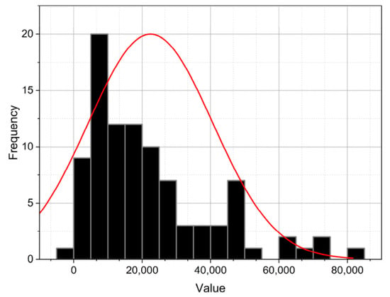
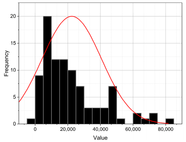
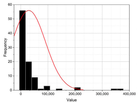
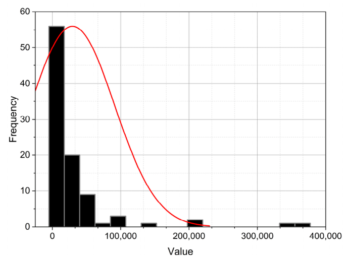
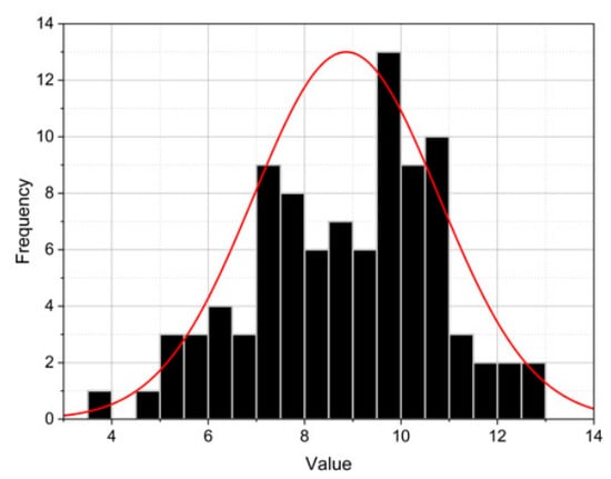
This coding scheme anonymizes proprietary information while enabling easy identification and tracking of each medication throughout the study. As an initial step, we performed exploratory data analysis using histograms, as shown in Figure 1 and Figure 2. These visualizations helped us inspect variable distributions in the dataset. Ideally, the data would follow a normal distribution, as this assumption benefits certain normalization techniques; however, examining the plotted distributions revealed that not all variables conformed to a Gaussian pattern.
Figure 1.
Histogram and Gaussian Distribution Curve of the Drug NS-0145053.
Figure 2.
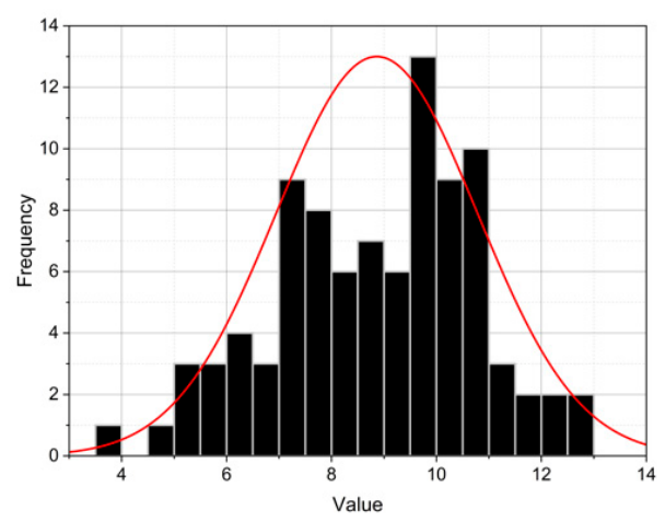
Histogram and Gaussian Distribution Curve of the Drug FO-0735011.
Because different normalization strategies have different advantages and disadvantages depending on the data type, we tested multiple scaling methods to find the most suitable one for this dataset. For this study, we processed the dataset using min-max normalization, logarithmic transformation, and robust normalization. We ultimately selected robust normalization given the dataset’s characteristics, including outliers and the absence of a clear behavioral pattern [40].
Robust normalization, used in addition to logarithmic normalization for this case, offers greater resistance to outliers compared to the min-max method; instead of relying on the extreme values (minimum and maximum), this technique utilizes statistical percentiles (typically the 25th and 75th percentiles), making it particularly suitable when the dataset contains significant outlier values [41].
The transformation follows a structure similar to min-max normalization. Still, it replaces the mean and full range with the median and interquartile range (IQR), providing more stable scaling in the presence of skewed data.
Logarithmic transformation is a valuable technique for data with strong positive skew, typically characterized by a long tail of high values. Applying a logarithm compresses larger values and reduces extreme differences, often resulting in a more symmetrical, less skewed distribution [42].
The fundamental transformation is expressed as:
X′ = log(X)
This method requires all input values to be strictly positive, since logarithms are undefined for zero or negative values. In cases where the dataset includes values close to or equal to zero, a shifted logarithmic transformation is commonly used, such as:
where c is a small constant added to prevent a singularity at zero. This method is especially effective when the data shows high variability, as it stabilizes variance and reduces the impact of extreme observations on the predictive model.
X′ = log(X + c)
Based on the histograms and distribution curves, most variables show a pronounced positive skew, with a dense concentration of values in the lower range and a long tail extending toward higher values. This skew indicates a deviation from normality, which can negatively affect neural network performance by letting disproportionately high values dominate training.
To address this asymmetry and reduce the influence of extreme observations, we selected a logarithmic transformation combined with robust normalization. This method compresses larger values, reduces variance, and balances low and high data points, enabling more efficient learning. By applying this transformation, the dataset’s distribution is expected to become more symmetrical, ultimately improving the model’s ability to capture meaningful patterns without being biased by outliers.
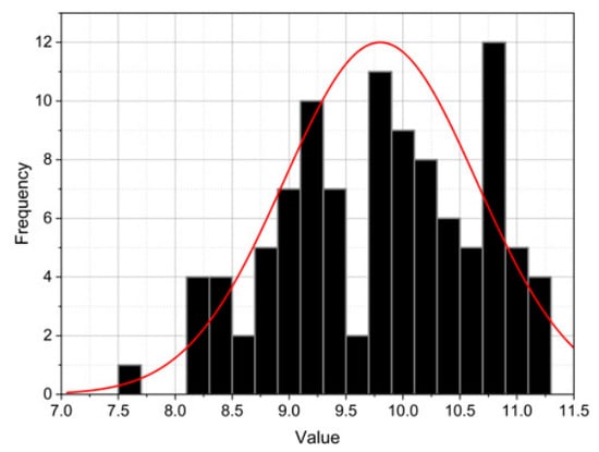
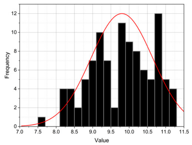
After normalizing the data, we created new histograms to show the adjusted value distributions for each medication. These visualizations include an overlaid normal distribution curve to make it easier to visually compare the normalized data with an ideal Gaussian distribution. This display helps evaluate how well normalization worked by showing how closely the transformed data matches a more symmetrical and statistically preferred distribution. Such alignment is crucial for ensuring the reliability of subsequent analyses, especially during neural network training and predictive model development. These results are illustrated in Figure 3 and Figure 4:
Figure 3.
Histogram and Gaussian Curve of the Drug FO-0735011.
Figure 4.
Histogram and Gaussian Curve of the Drug NS-0145053.
For medications with recorded returns, we applied a uniform shift of 1000 units to the historical sales data. This serves two purposes: first, it ensures that the neural network receives only positive values; second, it preserves the original data points rather than simply removing negative values. For instance, as shown in Figure 2, the data for oseltamivir phosphate (0735011) is right-skewed; to center this histogram, we applied logarithmic normalization—a method used for all medications with this characteristic. Conversely, for distributions that approximate a Gaussian curve, we applied min-max normalization. When the distribution contained highly random values and frequent outliers—such as the data for naproxen sodium (0145053), shown in Figure 1 and Figure 4—we used a robust normalization technique.
Table 3 summarizes the preprocessing methods applied to the sales data of the 13 pharmaceutical products evaluated in this study. We determined the preprocessing strategy based on each product’s sales distribution and the forecasting horizon (3, 6, or 12 months). As a result, the same pharmaceutical product may use different normalization methods depending on the forecasting period. The preprocessing methods included logarithmic transformation, RobustScaler, and Min–Max scaling. For oseltamivir phosphate products (FO), we used logarithmic transformation for certain forecasting horizons and Min–Max scaling for the 12-month horizon. For products with recorded negative sales values associated with returns, we added an offset of 1000 units to preserve the observations while ensuring positive values before transformation. We adopted this product- and horizon-specific preprocessing strategy to accommodate differences in sales distributions and the requirements of each forecasting horizon, improving the data’s suitability for neural network training.
Table 3.
Product-specific preprocessing methods and data adjustments applied to pharmaceutical sales datasets.
2.3. Neural Network Architecture
In neural networks, architecture refers to the model’s structural design, including how its layers are arranged and connected, as well as the operations performed within them. This setup determines how the network processes input data to produce outputs, allowing it to learn complex patterns from large amounts of information. In time series applications (such as forecasting pharmaceutical sales and managing inventory levels), the architecture is essential for capturing temporal dependencies and behavioral fluctuations, which directly affect the model’s predictive performance [43].
Before building the architecture, we took several preparatory steps to ensure a solid foundation. First, we imported the necessary libraries for data processing, visualization, and building the deep learning model. Next, we defined auxiliary functions to evaluate model performance using metrics like RMSE, Mean Absolute Error (MAE), and Mean Absolute Percentage Error (MAPE). We first reviewed the dataset, then transformed it into suitable time sequences for training and partitioned it into training and test sets [44]. Once the data was prepared, we established the hyperparameters that define the model’s structural configuration. Finally, we implemented the neural network, incorporating bidirectional LSTM layers, Transformer-type attention mechanisms, regularization methods, and dense layers, each of which is explained in more detail in the following subsections. This preparatory step establishes the necessary foundation for understanding the architecture and training strategy used in this study [45,46].
2.3.1. Data Preparation and Sequence Creation
The first step involved selecting all relevant columns from the data frame: seven key variables for the oseltamivir phosphate models (including infant mortality) and six for sodium naproxen (excluding the infant mortality rate). We also included historical sales of the corresponding medication as an input feature, resulting in eight input features for oseltamivir phosphate and seven for sodium naproxen. We extracted these and organized them into a matrix with the appropriate dimensions. We then divided the dataset into three chronologically ordered subsets: training, validation, and testing. We performed this partitioning before applying any scaling technique, ensuring that normalization parameters were derived solely from the training data. This method prevents data leakage by preventing the test set from influencing the training process and preserving the model’s ability to generalize.
We performed data preprocessing using the product-specific methods described in Section 2.2 and summarized in Table 3. Depending on each pharmaceutical product’s historical sales distribution, we applied logarithmic transformation, robust scaling, or Min–Max scaling. For products with recorded negative sales values associated with returns, we added an offset of 1000 units before the corresponding transformation, as shown in Table 3. To prevent data leakage, we estimated all data-dependent preprocessing parameters exclusively from the training subset. Then we applied them to the validation and test subsets. We maintained the same preprocessing configuration for each product throughout model training and evaluation. We transformed predictions back to their original sales units before calculating the cumulative forecasting errors reported in the results.
With the scaled data, the next step was to define the “create_multivariate_dataset” function, which generates temporal sequences from the normalized data matrix. This function iteratively traverses the time series, constructing consecutive data windows of a fixed length, called “look-back” steps. Each resulting sequence includes all input features, while the prediction target is taken from the first column, which represents the main output variable.
2.3.2. Sequential Input and Processing
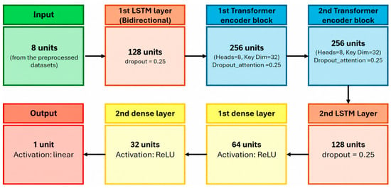
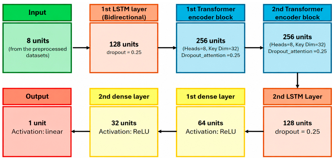
The architecture starts with an input layer shaped by the sequence length and number of features from the preprocessed datasets (8 input features for oseltamivir phosphate and 7 for sodium naproxen, comprising 7 and 6 external variables, respectively, plus the historical units sold for the corresponding medication.). This input passes through a bidirectional LSTM layer, which captures temporal dependencies in both forward and backward directions. Dropout and L2 regularization reduce overfitting and improve generalization; after the LSTM, two Transformer encoder blocks enhance the model’s ability to learn contextual relationships within the sequence. Each block includes a “MultiHeadAttention” layer with 8 heads and a key dimension of 32, followed by dropout, residual connections, and layer normalization. This layered design lets the model extract more detailed representations and refine them iteratively.
A subsequent LSTM layer with 128 units, combined with a “Global Average Pooling” operation, condenses the temporal information into a compact global representation. This step transitions to the dense layers, which consist of two fully connected layers with 64 and 32 units, respectively, both using ReLU activation, L2 regularization, and dropout.
Finally, the output layer is a fully connected layer with linear activation and an output size matching the selected forecasting horizon (3, 6, or 12 months). Each output neuron predicts the number of units sold for one future month, allowing the model to generate the entire forecasting sequence directly without recursively using previously predicted values. The diagram (Figure 5) illustrates the structure, showing the flow and interaction of each component within the proposed neural network.
Figure 5.
Neural Network Architecture Diagram.
2.3.3. Model Training and Optimization
The model training used Keras’s fit method, which allows iterative parameter adjustments on the training data while evaluating performance on a validation set [47]. A key part of this process is the “ReduceLROnPlateau” callback. This mechanism monitors the validation loss and, if it does not improve over five consecutive epochs, automatically lowers the learning rate by a factor of 0.5. This adaptive strategy helps avoid entrapment in local minima. It promotes convergence while ensuring the learning rate does not fall below a specified lower bound of 1 × 10⁻⁶.
The model was trained over 35 epochs with a batch size of 4. During each epoch, the network processes the multivariate sequences generated earlier in data preparation along with their corresponding target values. Validation uses an independent validation set chronologically separated from the training data, allowing real-time assessment of the model’s generalization performance and detection of overfitting risks. The ‘ReduceLROnPlateau’ callback monitors validation loss and automatically adjusts the learning rate when it stops improving. The test set, corresponding to the 2024 observations, remains completely independent of the training and validation procedures and is used only for the final model evaluation. This minimizes manual effort while improving training efficiency and the stability of the optimization process. The training phase depends heavily on careful data preprocessing, creating multivariate sequences, and the hybrid architecture that combines LSTM and Transformer modules.
3. Results
In this study, we evaluated the proposed model’s forecasting performance over 3-, 6-, and 12-month horizons to examine its behavior under short-, medium-, and long-term forecasting scenarios. These horizons provide a consistent framework for assessing how forecasting performance changes as the prediction period increases and for comparing model behavior across pharmaceutical products, with the 3-month horizon representing the short-term forecasting scenario, the 6-month horizon representing the medium-term scenario, and the 12-month horizon representing the long-term scenario. This organization enables a direct comparison of prediction accuracy across forecasting horizons. It provides a basis for identifying differences in model performance associated with product characteristics and increasing forecast length.
In each case, we omit the first predicted value to avoid bias from overlap with the most recent training data. This adjustment accounts for the delay between the end of the previous month’s sales and the start of forecasting, which is especially relevant when immediate manufacturing decisions are needed. For the 3-, 6-, and 12-month forecasting horizons, we employed a direct multi-output forecasting strategy. For each horizon, the model receives the historical sequence defined by the fixed look-back window and, in a single prediction, generates the full sequence of future values for the selected horizon (3, 6, or 12 months). Thus, forecasts are not generated recursively or through repeated one-step predictions, and the model does not feed previously predicted values back in. The architecture uses a single target output with multiple forecast steps, and it does not use future observed values of the target and exogenous variables as inputs during prediction. Consequently, each forecasting horizon represents an independent out-of-sample prediction based exclusively on the information available at the forecasting origin.
3.1. Experimentation and Comparison Between Optimizers
Given these considerations and the importance of sales volume in determining future inventory needs, we ran a series of experiments to generate 3-, 6-, and 12-month forecasts. For each prediction window, we used historical monthly data from January 2015 through 2023 to develop and validate the model, reserving the 2024 data exclusively for the final out-of-sample evaluation. There were three validation periods for the three-month window, two for the six-month window, and one for the 12-month window.
The following section presents the quantitative results of these experiments, highlighting improvements in error metrics across forecast windows under the four main optimizers used in the neural network model: Adam, RMSprop, Nadam, and SGD.
The results for each prediction window (3, 6, and 12 months) show consistent patterns in optimizer performance. Nadam performed best across the evaluated forecasting horizons, achieving the lowest MAPE and RMSE for the 3-month horizon and the lowest MAPE, MAE, and RMSE for the 6- and 12-month horizons.
This positive trend also held for the 12-month forecasts. However, over this longer prediction period, the optimizers’ differences were less noticeable in the error metrics. Still, Nadam’s higher accuracy in the predicted values further proves its effectiveness.
Table 4 provides a comparative summary of the quantitative results obtained for each optimizer across the different prediction horizons. The medications analyzed and the details of the architecture used are shown in Table 5. To clarify the apparent differences between the error metrics reported in Table 4 and the cumulative errors presented in Table 6, Table 7 and Table 8, these results correspond to two complementary evaluation procedures. The MAPE, MAE, and RMSE reported in Table 4 are computed from model predictions on the normalized scale used during model evaluation and are summarized across the forecasting observations. In contrast, the errors in Table 6, Table 7 and Table 8 are computed after reversing the preprocessing transformation and restoring the predictions to their original units. For the latter analysis, we accumulate actual and predicted sales over each 3-, 6-, or 12-month forecasting horizon, and compute the percentage error from the difference between these cumulative values. Therefore, the two approaches are not expected to produce equivalent numerical values: Table 4 evaluates point-level predictive error, while Table 6, Table 7 and Table 8 evaluate the accuracy of the total sales volume projected over each forecasting horizon.
Table 4.
Comparison of the results obtained for each optimizer.
Table 5.
Model implemented by medication.
Table 6.
Results obtained for a 3-month time window.
Table 7.
Results obtained for a 6-month time window.
Table 8.
Results obtained for a 12-month time window.
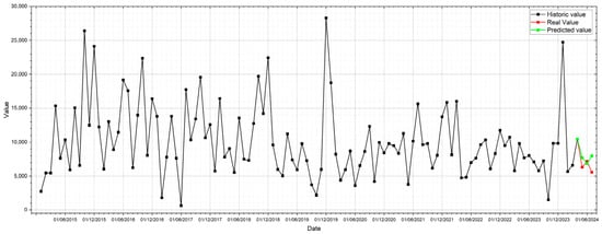
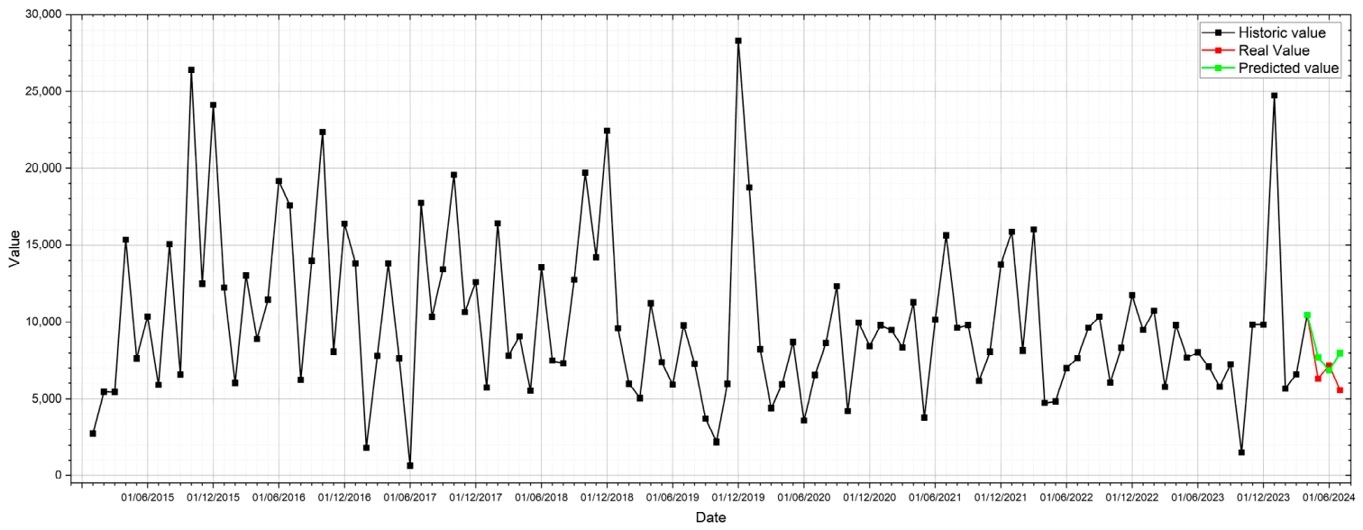
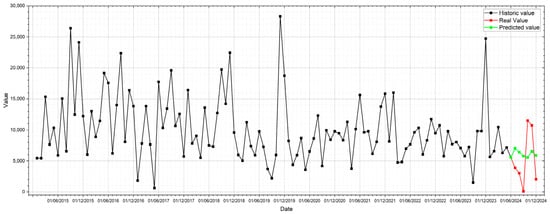
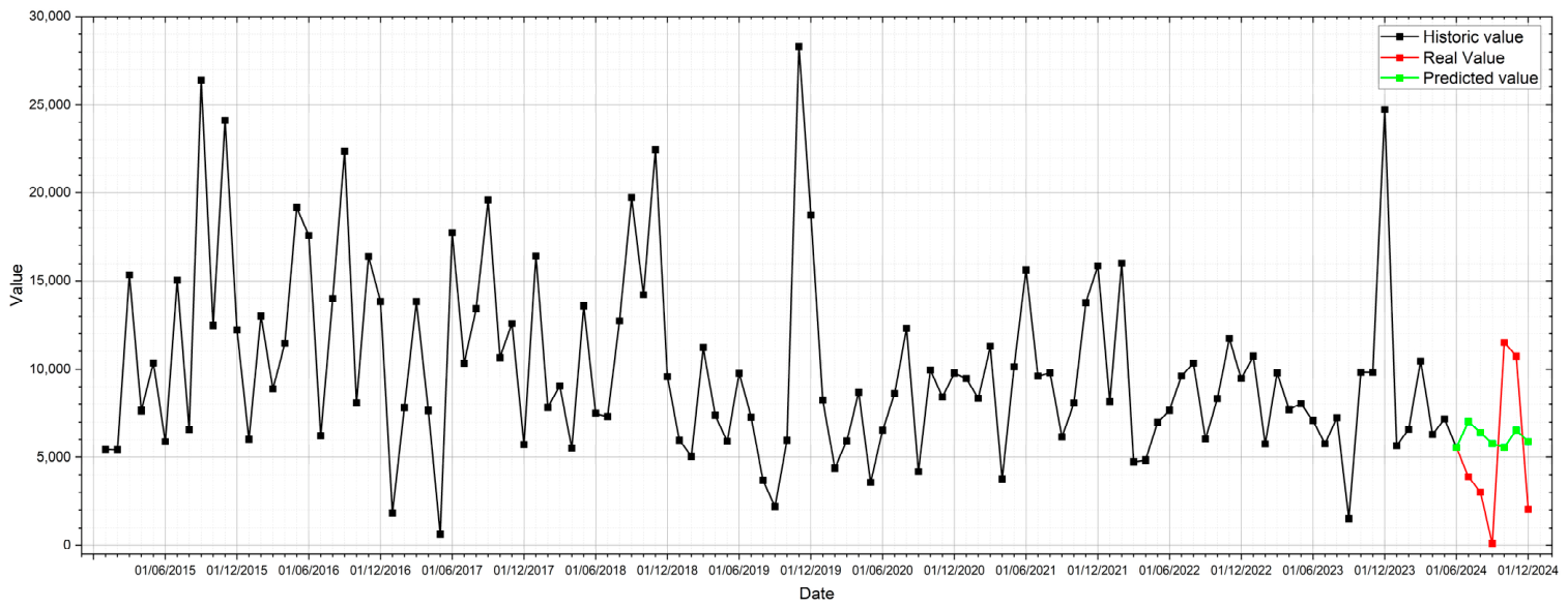
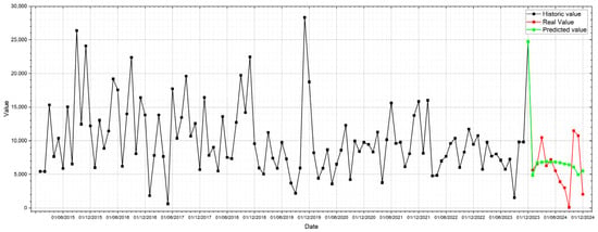
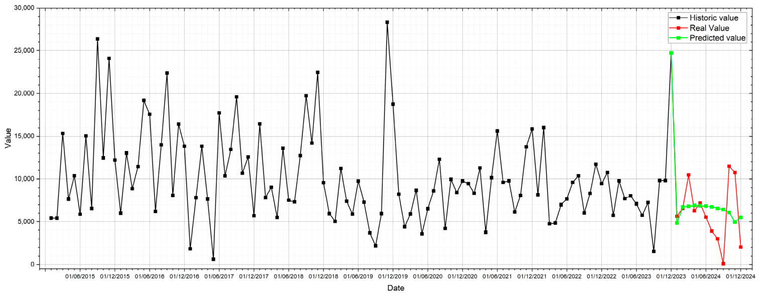
The following figures (Figure 6, Figure 7 and Figure 8) show comparative plots of actual values versus the model’s predictions for the 3-, 6-, and 12-month horizons, using the Nadam optimizer. These plots allow a visual assessment of the model’s performance across different timeframes.
Figure 6.
Three-month predictions with Nadam optimizer.
Figure 7.
Six-month predictions with Nadam optimizer.
Figure 8.
Twelve-month predictions with Nadam optimizer.
3.2. Models Based on the Type of Medication
During development, we analyzed 13 medications, as listed in Table 5. However, the main model produced satisfactory results only for the following sodium naproxen-based medications: NS-0145051, NS-0145052, NS-0145054, NS-0145055, NS-0161000, NS-0163001, and NS-0163000. In these cases, the neural network reliably forecast future unit sales, kept error rates low, and generalized well.
In contrast, applying the same modeling approach, even with hyperparameter adjustments, to FO-0735011, FO-0735012, and FO-0735013 (Oseltamivir Phosphate variants) resulted in a noticeable decline in prediction accuracy. This required adjustments to data preprocessing and model optimization, while maintaining the underlying hybrid BiLSTM–Transformer architecture. Major changes involved applying logarithmic normalization for the 3- and 6-month forecasting horizons and Min–Max scaling for the 12-month horizon, adding a 1000-unit offset only for products FO-0735011 and FO-0735012 to handle non-positive sales values associated with returns, switching to the Adam optimizer, and fine-tuning several hyperparameters. Additionally, three medications (NS-0148000, NS-0145053, and NS-0146016) consistently failed to produce reliable predictions with either model. Table 5 summarizes these findings.
3.3. Three-Month Forecasting Results
The analysis starts with evaluating the model in short-term scenarios, specifically using a rolling 3-month window. As noted earlier, this horizon is especially relevant for the private sector, where decision-making is often more dynamic and focused on short operating cycles. In this context, comparing cumulative predictions with actual values helps us assess the model’s accuracy under high error sensitivity.
Table 6 shows the results by medication, including the total error percentage for each case. Overall, the model performed adequately for most products tested, with low to moderate error rates in most instances. Medicines NS-0145054, NS-0145055, NS-0163000, and NS-0163001 stand out, showing relatively low error rates. This suggests the model can capture short-term demand patterns for these products, making it reliable for environments that require quick, precise planning. In contrast, the NS-0161000 medication showed a 16.88% error rate. Although higher than the others, this value could still be acceptable depending on the logistics context and the organization’s operating margins. However, FO-0735012 stands out negatively, with a 82.28% error, indicating a significant underestimation of actual demand. This unusual behavior suggests the model did not adequately capture its dynamics, possibly because of greater seasonal variability, nonlinear patterns, or insufficient representation in the training data.
3.4. Six-Month Forecasting Results
Model evaluation in medium-term scenarios, particularly with a 6-month forecast window, is especially important for institutional purchasing. In these settings, acquisitions are usually planned well in advance and require accurate estimates that account for both overall trends and potential seasonal variations. Like short-term analyses, the method relies on comparing accumulated values over the testing period. The model calculates totals of actual sales and forecasts for the six-month interval, enabling the calculation of both absolute and relative errors. These metrics clearly measure the model’s ability to capture demand behavior over an intermediate timeframe, where managing error margins is crucial for effective planning.
The results shown in Table 7 reveal a mixed accuracy pattern. Some medications have estimates very close to actual values, while others display significant deviations. A notable example is medication NS-0145051, which recorded an error rate of only 1.29%, showcasing the model’s strong predictive ability in this case. However, this good performance contrasts with less favorable results for NS-0148000 and FO-0735012, where errors increased to 74.47% and 81.11%, respectively, indicating a significant underestimation of actual demand.
Medications such as NS-0145052 and NS-0163000 had error rates of 23.09% and 25.36%, respectively. While these figures are not ideal, they indicate that the model can partially capture the demand dynamics in these cases. A notable exception is NS-0145053, which reached an error of 50.77%, highlighting a significant gap between predictions and actual sales during the period.
These results emphasize the need to further improve both the architecture and data processing, especially for medications with high volatility or less predictable consumption patterns.
3.5. Twelve-Month Forecasting Results
To conclude the analysis of the proposed model’s results, we assessed its predictive ability over a twelve-month long-term horizon. This scenario matters for strategic planning in the pharmaceutical industry, as critical decisions such as advance procurement of raw materials, large-scale production scheduling, and efficient inventory management depend on an extended outlook.
As with previous time windows, the analysis compares total actual sales during the testing period with the model’s predictions for the same period. The difference is then calculated in both absolute and percentage terms for each drug evaluated.
This evaluation type allows clearer identification of the model’s strengths and weaknesses over longer periods, which can be affected by pronounced seasonality, shifts in consumption patterns, or unexpected demand fluctuations.
The twelve-month prediction results, shown in Table 8, show mixed accuracy, similar to the six-month window trend. Some medications have highly accurate predictions, while others deviate notably from actual cumulative values.
In particular, NS-0161000 had a remarkably low margin of error of 1.77%, indicating that the model can maintain high accuracy even in long-term scenarios, as long as demand follows consistent patterns. Similarly, the drug FO-0735013 showed an acceptable error of 13.18%, suggesting good predictive performance.
However, some cases showed a significant loss of accuracy. For example, the drug FO-0735012 had an error of 155.83%, indicating substantial overestimation. This deviation suggests that some products have seasonal, abrupt, or nonlinear demand that the model cannot predict well over the long term.
Similarly, drugs NS-0163000 and NS-0145055 showed error rates of 28.62% and 18.71%, respectively, reinforcing the observation that model accuracy tends to decline as the prediction time horizon extends.
Ultimately, the results indicate that while the model can produce acceptable predictions in some cases, its long-term performance still has room for improvement. This limitation is particularly clear for medications with highly variable demand or those affected by external factors not included in training, as seen with different formulations of oseltamivir phosphate.
To evaluate the model’s results, we compare them against a baseline. In this case, we test the hypothesis that the medication’s sales behavior is seasonal, and we calculate the baseline using a Seasonal Naïve series. Table 9 show the comparison.
Table 9.
Comparison of observed and predicted cumulative pharmaceutical sales using the BiLSTM–Transformer and Seasonal Naïve models over the 3-month forecasting horizon.
The comparison between the BiLSTM–Transformer model and the Seasonal Naïve baseline across all 13 pharmaceutical products and the three forecasting horizons provides a more comprehensive assessment of their predictive performance (Table 9, Table 10 and Table 11). The results show that the proposed model achieves lower forecasting errors for 11 of the 13 products at the 3-month horizon, and for 9 of the 13 products at both the 6- and 12-month horizons. These findings suggest that the BiLSTM–Transformer model offers a predictive advantage for most products in this dataset, particularly for short-term forecasting. However, its performance is inconsistent across products and forecasting horizons.
Table 10.
Comparison of observed and predicted cumulative pharmaceutical sales using the BiLSTM–Transformer and Seasonal Naïve models over the 6-month forecasting horizon.
Table 11.
Comparison of observed and predicted cumulative pharmaceutical sales using the BiLSTM–Transformer and Seasonal Naïve models over the 12-month forecasting horizon.
At the 6-month horizon (Table 10), for example, the Seasonal Naïve baseline substantially outperforms the proposed model for FO-0735011 and FO-0735012. Similarly, at the 12-month horizon (Table 11), it achieves lower errors for several products, including FO-0735011, FO-0735012, FO-0735013, and NS-0146016. Notably, the BiLSTM–Transformer model exhibits particularly high errors for FO-0735011 at the 6- and 12-month horizons (109.99% and 317.08%, respectively) and for FO-0735012 across all three horizons, indicating that its predictive advantage does not generalize to every product or time scale.
The comparison with the Seasonal Naïve baseline reveals differences in forecasting performance across pharmaceutical products and forecasting horizons. Although the proposed BiLSTM–Transformer model achieved lower cumulative percentage errors for several medications, it did not consistently outperform the baseline in all evaluated cases. Nevertheless, the proposed model achieved lower cumulative percentage errors for several other products, including NS-0145051, NS-0145053, NS-0145054, and NS-0161000, across multiple horizons. These differences highlight the importance of product-specific demand characteristics and forecast horizon when selecting a forecasting approach. Although the present results do not establish a direct causal relationship between demand patterns and model performance, they suggest that the BiLSTM–Transformer model may be more suitable for products whose demand dynamics benefit from integrating historical information and external explanatory variables. In contrast, Seasonal Naïve may remain a preferable alternative when seasonal patterns provide a more reliable forecasting signal. Therefore, the proposed model’s practical value lies not in universal superiority over simpler baselines, but in its ability to improve predictive accuracy for a substantial proportion of the evaluated products. Model selection should therefore consider product-level performance and the intended forecasting horizon.
Beyond comparing the predictive performance of the proposed BiLSTM–Transformer model with the Seasonal Naïve baseline, it is also important to examine how individual input variables contribute to forecasting accuracy. In particular, infant mortality warrants further examination because, unlike the other explanatory variables, its original data are reported annually and then interpolated to match the dataset’s monthly granularity. Although this interpolation does not add empirical information, including this variable may affect the model’s predictive performance. Therefore, we conducted a sensitivity analysis to evaluate the effect of including or excluding infant mortality while maintaining the same evaluation procedure and comparable model configurations. The results of this analysis are presented in Table 12.
Table 12.
Sensitivity Analysis for FO-0735012, with different time windows for the infant mortality variable.
For product FO-0735012, the BiLSTM–Transformer model exhibits limited predictive performance across all three forecasting horizons, with the highest error observed at the 12-month horizon. Compared with the Seasonal Naïve approach, the proposed model yields error rates of 82.28%, 81.11%, and 155.83% for 3-, 6-, and 12-month horizons, respectively, whereas the Seasonal Naïve method yields error rates of 62.37%, 19.02%, and 9.17%. These results show that the Seasonal Naïve baseline consistently outperforms the proposed hybrid architecture for FO-0735012 across all three forecasting horizons, not just the shorter ones. Furthermore, sensitivity analysis indicates that excluding the infant mortality variable increases the model’s error for the 3-month horizon. These results suggest that the interpolated variable may contribute to short-term forecasting but does not consistently improve performance over longer horizons. Importantly, these findings are specific to FO-0735012 and the model configurations examined and should not be generalized to other pharmaceutical products without further evaluation. Moreover, the observed differences show the hybrid model’s relative underperformance compared with Seasonal Naïve, rather than establishing that demand for this product is inherently difficult to predict. Consequently, these findings highlight the need to assess the utility of external variables and select an appropriate model for the specific product and forecast horizon.
4. Discussion
For each case analyzed, we first calculated total actual sales for the period corresponding to the selected time window (3, 6, or 12 months). We then compared this value to the sum of the model’s predictions for the same interval. This comparison produces both the absolute difference and the cumulative error percentage, providing a clear view of the model’s ability to project total demand volumes under different scenarios.
This approach complements traditional point-by-point metrics by providing information on total demand volumes relevant to operations, logistics, and supply planning. Unlike indicators such as MAE or RMSE, which measure errors in individual predictions, cumulative analysis assesses overall unit projection accuracy, a vital factor in industries where decision-making relies on total volume rather than monthly precision.
In the pharmaceutical industry, where overproduction or shortages can be costly, cumulative accuracy becomes especially important. Production, raw material procurement, and logistics decisions rely on overall demand forecasts, so even small deviations in total numbers may have important implications for operational planning. Thus, the cumulative evaluation offers a measure that better matches real-world planning needs in industrial settings. The quantitative results are organized by prediction window (short-, medium-, and long-term), providing a clearer view of the model’s usefulness for practical decision-making.
Regarding the lack of precision in oseltamivir phosphate predictions, deep learning models, such as the proposed BiLSTM–Transformer architecture, learn temporal dependencies from patterns in the training data. Therefore, when a sudden demand increase is tied to an external event poorly represented in historical observations, the model may tend to reproduce the previously learned demand level rather than anticipate an abrupt change. This limitation may be particularly relevant for FO-0735012, because the observed demand of 36,030 units was considerably higher than the predicted value of 6383 units. Thus, the high error does not necessarily indicate a general weakness of the proposed model; rather, it highlights its limitation in capturing observed demand for this product under the evaluated conditions. This interpretation aligns with the Seasonal Naïve baseline achieving a lower forecasting error for FO-0735012, suggesting that the hybrid model’s predictive performance should be assessed relative to simpler forecasting approaches rather than attributing the observed error solely to demand complexity.
The forecasting results for FO-0735012 also indicate that incorporating epidemiological explanatory variables, such as influenza incidence and other respiratory infection indicators, did not ensure accurate demand predictions for this product. Although these variables may provide relevant context, including them does not necessarily enable the model to capture all factors influencing pharmaceutical demand. Furthermore, the Seasonal Naïve baseline’s superior performance for FO-0735012 suggests that increasing model complexity does not consistently improve forecasting accuracy. These findings highlight the importance of evaluating the contribution of explanatory variables and comparing alternative forecasting approaches for individual pharmaceutical products. Further analyses are needed to determine whether the observed errors relate to the available predictors, the data’s temporal characteristics, or the model configuration.
Although demand forecasting can inform pharmaceutical production planning, improved predictive accuracy does not automatically reduce overproduction or environmental impacts. Realizing these benefits depends on additional operational factors, including production flexibility, inventory management policies, procurement decisions, and manufacturers’ ability to adjust production volumes in response to forecasted demand. Furthermore, forecasting errors may lead to either excess inventory or product shortages, depending on their direction and magnitude. Therefore, interpret the potential sustainability implications of the proposed approach cautiously. The present study evaluates forecasting performance but does not directly quantify changes in production volumes, inventory levels, product expiration, waste generation, or environmental indicators. Assessing these outcomes would require integrating the forecasting model into a production planning framework and comparing its operational and environmental performance with existing planning practices.
The present study has several limitations to consider when interpreting its findings. First, forecasting performance varied across pharmaceutical products and prediction horizons, with substantial errors observed for certain medications, particularly those exhibiting irregular demand patterns. Second, the comparison with the Seasonal Naïve baseline revealed that a simpler forecasting approach may outperform the proposed hybrid architecture under specific conditions, limiting the generalizability of its predictive advantages. Third, interpolating monthly infant mortality data does not add independent empirical observations, and the sensitivity analysis for FO-0735012 does not show a consistent predictive benefit from including this variable. Finally, although the proposed model may inform production planning, it did not directly measure its potential effects on inventory management, overproduction, waste generation, or environmental sustainability. These limitations highlight the need for further comparative evaluations, sensitivity analyses, and operational assessments before drawing broader conclusions regarding the practical applicability and sustainability implications of the proposed approach.
5. Conclusions
This study developed a hybrid BiLSTM–Transformer model for pharmaceutical demand forecasting, using real-world industrial data and external epidemiological, climatic, demographic, and economic variables. We evaluated the model at 3-, 6-, and 12-month forecasting horizons. Results showed that forecasting performance depended strongly on both product characteristics and the prediction horizon. Short-term forecasts were the most consistent, with six of the thirteen evaluated products achieving cumulative errors below 10% over the three-month forecasting horizon. In contrast, medium- and long-term forecasts varied more. Compared with the Seasonal Naïve baseline, the proposed model achieved lower cumulative forecasting errors for 11 of 13 products at the 3-month horizon and 9 of 13 products at both the 6- and 12-month horizons, although the baseline performed better for certain products. Nadam generally produced the lowest forecasting errors, although products with irregular or highly volatile demand, particularly some oseltamivir formulations, remained more difficult to predict. These findings also highlight the importance of evaluating the contribution of explanatory variables and applying consistent validation procedures when comparing product-specific model configurations.
From a sustainability perspective, AI-based demand forecasting may provide useful information to better align pharmaceutical production with market demand. However, potential benefits, such as reductions in overproduction, excess inventory, storage requirements, product expiration, and stockouts, depend on subsequent production and inventory management decisions and were not directly evaluated in this study. The findings also indicate that a single forecasting configuration should not be applied universally across products. Future research should therefore integrate forecasting with production, inventory, environmental, and life-cycle indicators and compare forecast-based production planning with the company’s current planning approach to empirically assess these potential sustainability benefits. Overall, the proposed framework may serve as a data-driven decision-support tool for pharmaceutical production planning, provided that the model configuration is adapted to product characteristics and the forecasting horizon.
Author Contributions
A.-G.D.-I.: Writing—original draft, Validation, Methodology, Investigation. V.-B.M.V.: Formal analysis, Data curation. M.-C.J.: Writing—review & editing, Investigation. L.-G.Y.: Writing—review & editing, Supervision. A.-J.G.S.: Project administration, Funding acquisition, Conceptualization. F.G.-G.: Review & editing. C.-C.J.: Supervision, Funding acquisition. All authors have read and agreed to the published version of the manuscript.
Funding
This research is supported by the National Polytechnic Institute (Instituto Politécnico Nacional): IND-2026-0478, IND-2026-0714, SIP20260072, SIP 20260821, and SIP 20261012.
Institutional Review Board Statement
Not applicable.
Informed Consent Statement
Not applicable.
Data Availability Statement
The data in this article are not accessible due to the company’s confidentiality policies.
Acknowledgments
The authors thank the Secretaría de Investigación y Posgrado for their support.
Conflicts of Interest
The authors declare no conflicts of interest.
Abbreviations
The following abbreviations are used in this manuscript:
| BiLSTM | bidirectional long short-term memory |
| FO | Oseltamivir Phosphate formulations |
| IQR | interquartile range |
| LSTM | Long Short-Term Memory |
| MAE | Mean Absolute Error |
| MAPE | Mean Absolute Percentage Error |
| NS | Sodium Naproxen formulations |
| PSO | Particle Swarm Optimization |
| RMSE | Root Mean Square Error |
References
- Bocelli, M.; Bottani, E.; Volpi, A.; Solari, F.; Lysova, N.; Montanari, R. Exploring the Relationship between Routing Policies and Market Demand Heterogeneity: A Simulation Analysis with Different Hardware and Software Configurations in Traditional Warehouses. J. Ind. Inf. Integr. 2024, 40, 100634. [Google Scholar] [CrossRef] [Scilit]
- Hristov, V.D.; Saliev, D.N.; Slavov, D.V. Artificial Intelligence Systems for Warehouse Stock Control. In Proceedings of the 2022 8th International Conference on Energy Efficiency and Agricultural Engineering (EE&AE 2022), Ruse, Bulgaria, 30 June–2 July 2022. [Google Scholar] [CrossRef] [Scilit]
- Dhande, V.; Khwaja, F.; Gore, S.; Buktar, R. Optimization of Traditional Warehouse Management System Using Artificial Intelligence and Machine Learning. J. Emerg. Technol. Innov. Res. 2021, 8, 596–608. [Google Scholar]
- Sustrova, T. A Suitable Artificial Intelligence Model for Inventory Level Optimization. Trends Econ. Manag. 2016, 10, 48–55. [Google Scholar] [CrossRef] [Scilit]
- Osman, B.M.; Alinkeel, S.; Bhavshar, D. A Study On Role of Artificial Intelligence to Improve Inventory Management System. Int. Res. J. Mod. Eng. Technol. Sci. 2022, 4, 226–233. [Google Scholar]
- Merkuryeva, G.; Valberga, A.; Smirnov, A. Demand Forecasting in Pharmaceutical Supply Chains: A Case Study. Procedia Comput. Sci. 2019, 149, 3–10. [Google Scholar] [CrossRef] [Scilit]
- Feng, T.; Shi, Y.; Guo, Y.; Ji, Y.; Zeng, Z. Data-Driven Forecasting of Pharmaceutical Sales: Distinguishing Promotional vs. Daily Scenarios. Int. J. Data Min. Bioinform. 2025, 29, 1–26. [Google Scholar] [CrossRef] [Scilit]
- Samniang, W.; Shah, S.M.T.; Tun, Y.M.; Munawar, A.; K C, S. A Hybrid Grey Wolf Optimized eXtreme Gradient Boosting-Based Machine Learning Model for Hospital Pharmaceutical Demand Forecasting. Sci. Rep. 2026, 16, 13400. [Google Scholar] [CrossRef] [Scilit] [PubMed]
- Chen, X.; Lu, G.; Zhang, H.; Wan, J. Knowledge Graph-Enhanced Deep Learning for Pharmaceutical Demand Forecasting. Sci. Rep. 2026, 16, 4776. [Google Scholar] [CrossRef] [Scilit] [PubMed]
- Chen, J.; Yu, X.; Li, T.; Shen, S.; Guo, R.; He, J.; Wang, Z.; Chen, J.; Zeng, W. Comparative Performance of Multiple Predictive Models Constructed for Budesonide Nebulized Formulation Requirements. Front. Pharmacol. 2026, 17, 1937185. [Google Scholar] [CrossRef] [Scilit] [PubMed]
- Ramírez, F.G. Neural Multi-Quantile Forecasting for Optimal Inventory Management. arXiv 2021. [Google Scholar] [CrossRef] [Scilit]
- Artificial Neural Network Approach for Inventory Management Problem. Available online: https://www.researchgate.net/publication/375638886_Artificial_Neural_Network_Approach_for_Inventory_Management_Problem (accessed on 15 July 2025).
- Higuera Iglesias, A.L.; Kudo, K.; Manabe, T.; Corcho Berdugo, A.E.; Corrales Baeza, A.; Alfaro Ramos, L.; Guevara Gutiérrez, R.; Manjarrez Zavala, M.E.; Takasaki, J.; Izumi, S.; et al. Reducing Occurrence and Severity of Pneumonia Due to Pandemic H1N1 2009 by Early Oseltamivir Administration: A Retrospective Study in Mexico. PLoS ONE 2011, 6, e21838. [Google Scholar] [CrossRef] [Scilit] [PubMed]
- Davies, B.E. Pharmacokinetics of Oseltamivir: An Oral Antiviral for the Treatment and Prophylaxis of Influenza in Diverse Populations. J. Antimicrob. Chemother. 2010, 65, ii5–ii10. [Google Scholar] [CrossRef] [Scilit] [PubMed]
- Naproxen (Aleve, Naprosyn, Others): Uses, Side Effects, Interactions, Pictures, Warnings & Dosing—WebMD. Available online: https://www.webmd.com/drugs/2/drug-5173-1289/naproxen-oral/naproxen-oral/details (accessed on 15 July 2025).
- Treating Flu with Antiviral Drugs | Influenza (Flu) | CDC. Available online: https://www.cdc.gov/flu/treatment/antiviral-drugs.html (accessed on 15 July 2025).
- Aljuhani, O.; Korayem, G.B.; Altebainawi, A.F.; Alotaibi, M.S.; Alrakban, N.A.; Ghoneim, R.H.; Vishwakarma, R.; Al Shaya, A.I.; Al Harbi, S.; Gramish, J.; et al. The Effect of Oseltamivir Use in Critically Ill Patients with COVID-19: A Multicenter Propensity Score-Matched Study. Saudi Pharm. J. 2023, 31, 1210–1218. [Google Scholar] [CrossRef] [Scilit] [PubMed]
- Demand Forecasting Methods and Their Importance in 2026. Available online: https://www.impactanalytics.ai/blog/demand-forecasting-methods (accessed on 2 October 2026).
- Kalla, R.; Murikinjeri, S.; Abbaiah, R. An Improved Demand Forecasting with Limited Historical Sales Data. In Proceedings of the 2020 International Conference on Computer Communication and Informatics, ICCCI 2020, online, 26–28 June 2020. [Google Scholar] [CrossRef] [Scilit]
- Yu, C. Design of Drug Sales Forecasting Model Using Particle Swarm Optimization Neural Networks Model. Comput. Intell. Neurosci. 2022, 2022, 6836524. [Google Scholar] [CrossRef] [Scilit] [PubMed]
- Eldred, M.E.; Thatcher, J.; Rehman, A.; Gee, I.; Suboyin, A. Leveraging AI for Inventory Management and Accurate Forecast—An Industrial Field Study. In Proceedings of the SPE Symposium Leveraging Artificial Intelligence to Shape the Future of the Energy Industry, Al Khobar, Saudi Arabia, 17–18 January 2023. [Google Scholar]
- Liu, J.; Wu, X.; Feng, Y. Drug Purchase Prediction Model Algorithm. In Proceedings of the 2022 5th International Conference on Advanced Electronic Materials, Computers and Software Engineering (AEMCSE); IEEE: New York, NY, USA, 2022; pp. 392–396. [Google Scholar]
- Abolghasemi, M.; Hurley, J.; Eshragh, A.; Fahimnia, B. Demand Forecasting in the Presence of Systematic Events: Cases in Capturing Sales Promotions. Int. J. Prod. Econ. 2020, 230, 107892. [Google Scholar] [CrossRef] [Scilit]
- Madureira, L.; Popovič, A.; Castelli, M. Competitive Intelligence: A Unified View and Modular Definition. Technol. Forecast. Soc. Change 2021, 173, 121086. [Google Scholar] [CrossRef] [Scilit]
- Bao, W.; Cao, Y.; Yang, Y.; Che, H.; Huang, J.; Wen, S. Data-Driven Stock Forecasting Models Based on Neural Networks: A Review. Inf. Fusion 2025, 113, 102616. [Google Scholar] [CrossRef] [Scilit]
- Tang, Y.M.; Chau, K.Y.; Lau, Y.Y.; Zheng, Z. Data-Intensive Inventory Forecasting with Artificial Intelligence Models for Cross-Border E-Commerce Service Automation. Appl. Sci. 2023, 13, 3051. [Google Scholar] [CrossRef] [Scilit]
- Malosh, R.E.; Martin, E.T.; Heikkinen, T.; Brooks, W.A.; Whitley, R.J.; Monto, A.S. Efficacy and Safety of Oseltamivir in Children: Systematic Review and Individual Patient Data Meta-Analysis of Randomized Controlled Trials. Clin. Infect. Dis. 2018, 66, 1492–1500. [Google Scholar] [CrossRef] [Scilit] [PubMed]
- The Future of Pharma Forecasting | Evaluate. Available online: https://www.evaluate.com/blog/the-future-of-pharma-forecasting/ (accessed on 2 October 2026).
- Role of Forecasting in The Global Pharmaceutical Industry | Cliniminds. Available online: https://cliniminds.com/blogs/role-of-forecasting-in-the-global-pharmaceutical-industry-38 (accessed on 2 October 2026).
- Vázquez-Narváez, J.A.; Rochín-Kobashi, I.A.; García-Robles, M.B.; Delgado-Roche, L. Efectividad y Seguridad de Oseltamivir En Suspensión En Pacientes Pediátricos Con Influenza o Enfermedad Tipo Influenza. Rev. Mex. De Pediatría 2023, 90, 176–179. [Google Scholar] [CrossRef] [Scilit] [PubMed]
- Nyoni, S.P.; Nyoni, T. Forecasting Infant Mortality Rate in Burkina Fasso Using Artificial Neural Networks. Int. Res. J. Innov. Eng. Technol. 2021, 5, 419–423. [Google Scholar]
- Adeyinka, D.A.; Muhajarine, N. Time Series Prediction of Under-Five Mortality Rates for Nigeria: Comparative Analysis of Artificial Neural Networks, Holt-Winters Exponential Smoothing and Autoregressive Integrated Moving Average Models. BMC Med. Res. Methodol. 2020, 20, 292. [Google Scholar] [CrossRef] [Scilit] [PubMed]
- Petneházi, G.; Gáll, J. Mortality Rate Forecasting: Can Recurrent Neural Networks Beat the Lee-Carter Model? arXiv 2019. [Google Scholar] [CrossRef] [Scilit]
- Mortality Rate, Infant (per 1,000 Live Births)—Mexico | Data. Available online: https://data.worldbank.org/indicator/SP.DYN.IMRT.IN?end=2022&locations=MX&start=2018 (accessed on 22 June 2024).
- Sujon, K.M.; Hassan, R.; Towshi, Z.T.; Othman, M.A.; Samad, M.A.; Choi, K. When to Use Standardization and Normalization: Empirical Evidence From Machine Learning Models and XAI. IEEE Access 2024, 12, 135300–135314. [Google Scholar] [CrossRef] [Scilit]
- Starovoitov, V.V.; Golub, Y.I. Data Normalization in Machine Learning. Informatika 2021, 18, 83–96. [Google Scholar] [CrossRef] [Scilit]
- Huang, L.; Qin, J.; Zhou, Y.; Zhu, F.; Liu, L.; Shao, L. Normalization Techniques in Training DNNs: Methodology, Analysis and Application. IEEE Trans. Pattern Anal. Mach. Intell. 2023, 45, 10173–10196. [Google Scholar] [CrossRef] [Scilit] [PubMed]
- 10.3 Feature Scaling via Standard Normalization. Available online: https://kenndanielso.github.io/mlrefined/blog_posts/10_Linear_multiclass_classification/10_3_Feature_scaling.html (accessed on 2 October 2026).
- Prater, R.; Hanne, T.; Dornberger, R. Generalized Performance of LSTM in Time-Series Forecasting. Appl. Artif. Intell. 2024, 38, e2377510. [Google Scholar] [CrossRef] [Scilit]
- Marques, H.O.; Campello, R.; Zimek, A.; Rothlauf, F. Robust Statistical Scaling of Outlier Scores: Improving the Quality of Outlier Probabilities for Outliers (Extended Version). In Proceedings of the 17th International Conference, SISAP 2024, Providence, RI, USA, 4–6 November 2024; Springer: Berlin/Heidelberg, Germany, 2024. [Google Scholar]
- Raymaekers, J.; Rousseeuw, P.J. Transforming Variables to Central Normality. Mach. Learn. 2024, 113, 4953–4975. [Google Scholar] [CrossRef] [Scilit]
- Castro Morales, U.M. Pronóstico de Ventas a Corto Plazo En El Sector de Consumo Masivo a Través de Modelos de Machine Learning. 2024. Available online: https://repositorio.uniandes.edu.co/entities/publication/4a60c5ef-2a11-4f1a-91e2-d64ebe91591f (accessed on 15 July 2025).
- Lara-Benítez, P.; Carranza-García, M.; Riquelme, J.C. An Experimental Review on Deep Learning Architectures for Time Series Forecasting. Int. J. Neural Syst. 2021, 31, 2130001. [Google Scholar] [CrossRef] [Scilit] [PubMed]
- Zhang, L.; Wang, R.; Li, Z.; Li, J.; Ge, Y.; Wa, S.; Huang, S.; Lv, C. Time-Series Neural Network: A High-Accuracy Time-Series Forecasting Method Based on Kernel Filter and Time Attention. Information 2023, 14, 500. [Google Scholar] [CrossRef] [Scilit]
- Caetano, R.; Oliveira, J.M.; Ramos, P. Transformer-Based Models for Probabilistic Time Series Forecasting with Explanatory Variables. Mathematics 2025, 13, 814. [Google Scholar] [CrossRef] [Scilit]
- Kamalov, F.; Zicmane, I.; Safaraliev, M.; Smail, L.; Senyuk, M.; Matrenin, P. Attention-Based Load Forecasting with Bidirectional Finetuning. Energies 2024, 17, 4699. [Google Scholar] [CrossRef] [Scilit]
- Wang, K.; Dou, Y.; Sun, T.; Qiao, P.; Wen, D. An Automatic Learning Rate Decay Strategy for Stochastic Gradient Descent Optimization Methods in Neural Networks. Int. J. Intell. Syst. 2022, 37, 7334–7355. [Google Scholar] [CrossRef] [Scilit]

Disclaimer/Publisher’s Note: The statements, opinions and data contained in all publications are solely those of the individual author(s) and contributor(s) and not of MDPI and/or the editor(s). MDPI and/or the editor(s) disclaim responsibility for any injury to people or property resulting from any ideas, methods, instructions or products referred to in the content. |
© 2026 by the authors. Licensee MDPI, Basel, Switzerland. This article is an open access article distributed under the terms and conditions of the Creative Commons Attribution (CC BY) license.