


Abstract
The resilience and stability of industrial supply chains are the core pillars of the sustainable development of the global economy, and also an important foundation for achieving the United Nations Sustainable Development Goals of “Responsible Consumption and Production” and “Industry, Innovation and Infrastructure”. To address the problem that traditional industrial supply chain risk assessment systems have fixed indicators and static weights, which are difficult to adapt to complex scenarios such as dynamic adjustments of supply chain nodes, fluctuations in market demand and changes in geopolitical patterns, and thus restrict the construction of sustainable supply chain resilience, this paper proposes a comprehensive indicator-weight dynamic evolution algorithm for industrial supply chain risk assessment systems. Firstly, the evolutionary characteristics and trigger rules of the industrial supply chain risk system are defined. Indicator-weight evolution is performed when the original indicator system can no longer meet the evaluation requirements. The Delphi method combined with the actual risk characteristics of the supply chain is adopted to determine the candidate indicator set. The candidate indicators are screened using the grey relational analysis algorithm and the entropy weight-variation coefficient method to construct the evolved risk indicator set. Secondly, an improved DEMATEL model is used to analyze the causal relationships among the evolved indicators. Evolutionary analysis of the original indicator weights is carried out according to the influence degrees between indicators, so as to obtain the evolved indicator weights and realize the dynamic linkage update of evaluation weights. This study conducts a case analysis using publicly available aggregated synthetic data on supply chain disruptions and resilience and compares the proposed method with the entropy weight–analytic hierarchy process (EW-AHP) and dynamic Bayesian network (DBN) methods. The performance of the methods is evaluated in terms of the consistency of indicator weights or relative importance, computational time, out-of-sample prediction performance, and retrospective analysis of a representative disruption event scenario. The results indicate that, under the current case and parameter settings, the proposed method can reconstruct the risk indicator system and coordinate indicator and weight updates, demonstrating certain advantages in computational efficiency and risk factor identification in the specified comparative experiments. It should be noted, however, that the current validation relies primarily on publicly available synthetic aggregated data and retrospective event-scenario analysis. Therefore, the evidence is insufficient to directly establish the risk-warning benefits or improvements in operational response efficiency that the method might deliver in real-world enterprise settings. This study provides a methodological framework for the coordinated updating of indicators and weights in dynamic industrial supply chain risk assessment. Its applicability across industries and practical effectiveness require further validation using independent data sources and actual enterprise operational data.
1. Introduction
Industrial supply chain risk assessment systems serve as the core technical support for ensuring supply chain resilience and stability and achieving sustainable development of the industrial chain. The adaptability and scientific rationality of a system’s indicators and weights directly determine the effectiveness of assessment results, thereby affecting the long-term sustainable operation capacity of enterprises as well as the security and stability of supply chains. Traditional assessment systems use fixed indicators and static weights, which fail to meet the evaluation requirements of dynamic scenarios such as supply chain node adjustment, transportation mode changes, and policy iteration. This easily leads to deviations in risk assessment and does not easily satisfy the practical demands of full-life-cycle risk management and control for modern industrial supply chains [1]. Therefore, constructing an indicator-weight evolution system that can be dynamically adjusted along with the development of supply chains is of great theoretical value and practical significance for enhancing the risk resistance of industrial supply chains and ensuring the security and stability of industrial chains and supply chains.
Currently, domestic and foreign scholars have conducted extensive research on industrial supply chain risk assessment, forming a rich theoretical and methodological system.
In terms of supply chain risk assessment, Lyu J et al. [2] constructed a dynamic comprehensive evaluation model based on complex network theory to assess the importance of unexpected risks at global soybean supply chain network nodes, confirming the core positioning of key nodes through empirical analysis and the 2SLS method to address endogeneity. Dong et al. [3] integrated fuzzy logic and the entropy weight method to establish a risk assessment model for cross-border e-commerce logistics supply chains, realizing quantitative evaluation of multi-dimensional risks via a four-layer framework. Ampofoah et al. [4] explored the path of AI/ML models in generating supplier risk scores, verifying the superiority of text-enhanced models in risk prediction through case studies. Lyu C et al. [5] proposed a dual-objective optimization method combining Bayesian networks and information theory to solve the interruption risk management problem of multi-level supply networks under data scarcity. Xiang et al. [6] built a hybrid hesitant fuzzy DEMATEL-entropy weight coefficient of variation model to comprehensively evaluate low-carbon automotive supply chain risks and the correlation between factors.
The above studies have contributed to the improvement of supply chain risk assessment systems, but they have fundamental limitations in the aspect of dynamic evolution. Existing models generally adopt a preset static indicator system and one-time weight calculation mode. Whether it is the traditional entropy weight method, DEMATEL method or emerging machine learning models, none have established an active trigger mechanism based on environmental changes, and thus cannot update the risk indicator library in real time in response to external shocks such as geopolitical conflicts and policy adjustments. Meanwhile, these methods can only calculate static weights within a fixed indicator framework, ignoring the dynamic evolution of causal transmission relationships between indicators, and failing to realize the coordinated linkage between indicator addition/deletion and weight adjustment. This leads to problems such as incomplete coverage of risk factors, delayed weight updating and inaccurate evaluation results when facing rapidly changing situations.
Regarding the evolution of indicators and weights, MengLi et al. [7] coupled the ABCD hydrological model with deep learning algorithms to quantitatively assess the impact of human activities and climate change on hydrological drought evolution. ZhenCao et al. [8] used Sen’s slope trend test and interpretable machine learning models to reveal the spatiotemporal evolution rules and driving mechanisms of GPP, ET, and WUE in the Yellow River Basin. TingtingLiu [9] applied the entropy weight TOPSIS model combined with spatial analysis methods to realize dynamic measurement and regional difference analysis of food security levels in 30 provinces. MinhuaLu [10] constructed a multi-dimensional indicator framework and used the entropy method to reveal the evolutionary law of new quality productive forces driving sustainable development. ShuWang et al. [11], using a base DPSIR model combined with entropy weight TOPSIS and a Markov transition matrix, analyzed the spatiotemporal evolution characteristics and driving factors of tourism ecological security in the Silk Road Economic Belt.
It should be noted that the above evolutionary studies in hydrology, ecology, food security and other fields mainly focus on retrospective analysis of the spatiotemporal evolution laws of objective phenomena, aiming to reveal historical change trends and driving mechanisms. Their indicator systems are mostly pre-determined and relatively stable throughout the research period, and weight adjustments are usually performed periodically based on overall data characteristics rather than real-time response to sudden changes. These methods are suitable for characterizing the evolution of natural or socioeconomic systems with relatively slow rates of change. However, they cannot be directly applied to industrial supply chain risk assessment scenarios that require real-time dynamic sensing and rapid response capabilities, nor can they adequately address the rapid reconstruction of assessment systems in response to structural disruptions in supply chains.
Furthermore, recent studies have introduced optimal transport methods into supply chain structural analysis, providing a novel perspective on supply chain efficiency diagnosis. A geometric optimal transport-based analytical framework for sustainable closed-loop supply chains has been proposed, employing the Gromov–Wasserstein distance to jointly assess supply chain structure and attribute efficiency, thereby providing a quantitative tool for supply chain structural optimization [12]. While these studies focus on the static evaluation of supply chain structural efficiency, the present study investigates the dynamic evolution of risk assessment systems. Thus, the two approaches complement each other by advancing supply chain management methodologies from different perspectives.
In summary, numerous scholars have conducted extensive research on the management, diversification, and informatization of industrial supply chains. However, there are still significant shortcomings in the study of indicator-weight co-evolution models for complex scenarios, which are difficult to adapt to the dynamic evolution characteristics of industrial supply chains. This study focuses on addressing two key issues:
(1) How to construct a risk indicator set that dynamically adapts to changing supply chain conditions, enabling the proactive addition and removal of indicators and their dynamic adaptation to evolving risk profiles;
(2) How to establish a dynamic weight updating mechanism based on the interactions among indicators to realize the co-evolution of indicators and weights.
To address the aforementioned issues, this paper proposes an innovative comprehensive dynamic-evolution algorithm for the index-weight system of industrial supply chain risk assessment. Its core innovation lies in the construction of a complete two-stage “trigger-reconstruction” evolution framework, which breaks through the inherent limitation of traditional static assessment models—a fixed index set with one-time weight calculation. The specific contributions are outlined as follows:
(1) A quantitative dynamic evolution trigger mechanism is established. It realizes active perception of supply chain system changes, solving the problem that traditional static models fail to respond to external environmental shocks in real time.
(2) An index evolution screening method coupled with Delphi-GRA-entropy weight-coefficient of variation is constructed. From the dual dimensions of correlation and information contribution, it achieves dynamic addition and deletion of assessment indicators, ensuring that the index system can be dynamically adapted to changes in supply chain scenarios.
(3) The standard DEMATEL method is extended for dynamic index scenarios. A weight redistribution mechanism based on inter-index causal correlation degree is proposed, which realizes smooth linkage update of weights after index addition or deletion, and avoids the high cost of full-scale remodeling and recalculation in traditional methods.
Validated with independent samples across multiple industries, the evolutionary algorithm proposed in this paper exhibits strong generalizability and consistency. In contrast to most existing studies that focus on static weight calculation under a fixed index system, this paper forms a complete closed-loop dynamic assessment system covering trigger judgment, index reconstruction and weight updates, providing a new methodological approach for dynamic risk assessment of sustainable industrial supply chains.
2. Description of the Characteristics and Evolutionary Forms of the Industrial Supply Chain System
2.1. Characteristics of the Industrial Supply Chain System
The primary task of industrial supply chain management is to construct a resilient supply chain system featuring end-to-end visibility, full-domain collaboration, and full-process controllability, in response to global market competition, industrial chain restructuring, and changes in the geopolitical landscape. It enables autonomous completion of various risk assessments and response decision-making, achieves high integration between the supply chain system and production and operation systems, and fully meets industrial production security requirements under a dynamic market environment. With the development of intelligence and flexibility in industrial manufacturing, the models and demands of industrial supply chains have also undergone corresponding changes. As the basis for subsequent risk control and optimization efforts, the industrial supply chain risk assessment system represents a critical link in supply chain resilience management.
Functionally, the industrial supply chain system is characterized by dynamic and variable task scenarios, continuously adjusted indicators, and a high degree of digital dependence [13]. In the actual operation of supply chains and risk control processes, with the replacement of core suppliers, adjustments to logistics and transportation routes, and constant changes in market demand, the evaluation indicators for industrial supply chain risk assessment are continuously evolving and updating, leading to certain complexity and fuzziness in their evaluation. Consequently, industrial supply chain risk assessment is inherently an evolutionary and dynamic process. As task scenarios change and supply chain entities are replaced, evaluation indicators are continuously added, deleted, or merged, with their weights changing accordingly.
2.2. The Triggering Mode of Industrial Supply Chain System Evolution
The industrial supply chain system represents a state of system operation under the combined effect of changing demands and entities. During the development of the industrial supply chain system, it evolves accordingly with task shifts and market updates. Therefore, the evolution of the industrial supply chain system can be interpreted as major changes occurring in the supply chain over continuous time, leading to alterations in its overall structure, resource allocation, and evaluation indicators. As the supply chain system transitions from one operational state to another, the collaborative evolution of indicators and weights is triggered accordingly.
To quantify the evolution trigger rules, the following rules are proposed:
1. Benchmark Period: The period during which the supply chain system operates stably following the previous indicator-weight evolution. Each time a full evolution is accomplished, the benchmark period is updated to the first cycle of stable operation of the system after evolution.
2. Monitoring Window: This window is consistent with the minimum unit of the benchmark period. Only the average value of each indicator within the window is calculated to avoid triggering evolution due to accidental random fluctuations.
3. Trigger Cooling Period: The minimum evolution interval is set to two monitoring window cycles. Evolution will not be triggered within the cooling period even if the threshold is reached.
Based on the calculation rules set above, the abnormal change value is calculated every monitoring window period. When the overall abnormal change value of the supply chain is excessively large, collaborative evolution is triggered. The calculation formula of the abnormal change value is as follows:
where m denotes the number of monitoring indicators, represents the weight of the monitoring indicator, is the standardized value of the j-th indicator within the monitoring window, and is the standardized mean value of the j-th indicator during the benchmark period.
The threshold is set at 0.6. This value strictly follows the empirically validated general risk classification standard for industrial supply chain risk assessment [14]. Based on the retrospective analysis of more than 1200 typical supply chain disruption events worldwide and industry consensus, this standard divides the supply chain system risk level into three intervals with clear management implications: low risk (0–0.3); medium risk (0.3–0.6); and high risk (≥0.6).
Building on the aforementioned risk classification, this study further conducts a sensitivity analysis of five candidate thresholds: 0.50, 0.55, 0.60, 0.65, and 0.70. This range was selected for the following reasons: thresholds below 0.50 may lead to normal local fluctuations being misclassified as systemic changes, whereas thresholds above 0.70 may delay responses to structural risks. Therefore, the range of 0.50–0.70 covers the primary decision-making spectrum from relatively sensitive to relatively conservative settings. The results indicate that a threshold of 0.60 provides a favorable balance among information retention, system redundancy, and risk response timeliness.
It should be noted that the threshold of 0.60 was not determined solely on the basis of the proposed method’s own composite score. Instead, it was further validated using external risk events independent of the threshold optimization process. Specifically, the 2024 Red Sea shipping disruption was selected as an external validation scenario, with the occurrence of the event and objective operational changes before and after the event serving as reference points. The results show that, at a threshold of 0.60, the model can identify a sustained increase in risk levels before the event occurs and trigger the coordinated evolution of indicators and their weights. Lower thresholds tend to increase false triggers during non-event periods, whereas higher thresholds may delay risk identification. Accordingly, 0.60 was ultimately selected as the evolution trigger threshold in this study. Empirical data from reference [14] shows that under the threshold of 0.6, the false trigger rate can be controlled within 8% and the missed trigger rate is less than 5%, which is the optimal value balancing assessment timeliness and system stability. Meanwhile, it is consistent with the critical values adopted in similar dynamic risk assessment studies by Guo et al. [14] and Lyu et al. [2], and has extensive academic consensus. The suitability of this threshold was further assessed through sensitivity analysis, with detailed results presented in Appendix A.
2.3. Overall Indicator-Weight Evolution Model for Industrial Supply Chain Risk Assessment
This study designs a two-stage technical route of “trigger-reconfiguration” focusing on the dynamic evolution of indicators and weights in the industrial supply chain system, with the specific process as follows:
First, the system enters the trigger phase, calculates the abnormal value of the supply chain risk assessment system according to the rules, and enters the evolution phase when the abnormal value exceeds the threshold.
The system enters the indicator and weight evolution phase, which is divided into two modules: indicator evolution, and weight update. In the indicator reconstruction module, first, according to changes in the external environment and policy updates, the Delphi method is adopted to determine candidate indicators. It combines the original indicator system with candidate indicators to construct a new indicator system, and uses the Grey Relational Analysis (GRA) algorithm to complete indicator screening and realize indicator addition. The entropy weight-coefficient of variation method is used to couple the screening logic of important indicators to complete indicator deletion and finally form an evolutionary indicator system. In the weight update module, the improved DEMATEL model is used to conduct evolutionary analysis on the addition and deletion of weights. The causal relationships between indicators are obtained through the DEMATEL algorithm, and weight allocation is performed according to the comprehensive impact matrix.
Through the above phased and modular technical processes, the dynamic evolution of indicators and weights in the industrial supply chain system is realized, providing methodological support for the adaptive optimization of the system. The overall structure of the evolution and reconfiguration of indicator-weight sets for industrial supply chain risk assessment in dynamic scenarios is shown in Figure 1 below:
Figure 1.
Evolution model of industrial supply chain system.
3. Indicator Evolution Model for Industrial Supply Chain Risk Assessment System
Indicator evolution serves as the prerequisite and foundation for updating the indicator weights in the industrial supply chain risk assessment system. To accurately evaluate the performance of the industrial supply chain risk assessment system under the constant changes in practical demands and supply chain entities, it is necessary to design corresponding models and algorithms to reconstruct the indicators. Specifically, models are constructed and restructured to accommodate the addition and deletion of indicators in the updated evaluation indicator set, enabling timely and accurate assessment of the supply chain risk system under dynamic scenarios. This provides a reference and guidance for subsequent risk judgment and precise management and control [15].
The composition of the risk evaluation indicator set changes dynamically with the evolution of the industrial supply chain system. Let the initial indicator system be . Then, at the i-th moment, the supply chain risk assessment indicator set is expressed as:
With the dynamic evolution of the industrial supply chain system, at the (i + 1)-th moment, the supply chain risk evaluation indicator set is:
In the indicator evolution process, an expert panel is first established using the Delphi method to conduct analysis and multiple rounds of anonymous voting on changes in the external environment of the supply chain, policy adjustments, and other relevant factors, ultimately obtaining candidate indicators for potential addition to the system. The grey relational analysis (GRA) algorithm is then employed to perform grey relational screening on the candidate indicators, eliminating those with low correlation to supply chain risk assessment. Finally, indicators that pass the correlation test are incorporated into the original indicator system. Concurrently, the entropy weight-variation coefficient method is applied to remove redundant indicators with low comprehensive contribution from the indicator system, resulting in the final evolved evaluation indicator system.
3.1. Addition of Evaluation Indicators
The Delphi Method is an expert collaborative decision-making approach based on multi-round anonymous consultation, feedback iteration and statistical aggregation, which can systematically integrate expert wisdom to form scientific and reliable decision conclusions [16]. The use of Delphi method in the dynamic evolution process of an industrial supply chain system can supplement the shortcomings of the original indicator system, adapt the systems to new supply chain environment and policy standards, and obtain the evaluation indicators that need to be added.
This study consulted five experts, including three academic researchers and two industry experts with experience in supply chain risk management in manufacturing enterprises. This expert panel provides professional judgment for the context-specific construction of the indicator system. However, the judgments obtained may be influenced by differences in individual professional backgrounds, industry experience, and risk perceptions. Therefore, expert opinions are used as a professional basis for candidate indicator identification and causal relationship analysis among indicators, rather than being treated as a statistical sample representative of the entire population of industrial supply chain experts. To examine the potential effects of variations in expert panel size on the analytical results, we conducted an exploratory sensitivity analysis using the existing five experts, comparing indicator evaluations and weight estimates across panels of three, four, and five experts. The purpose of this analysis is to identify potential differences arising from changes in the composition of the current expert panel, rather than to demonstrate the statistical stability or general applicability of the weight estimates across a larger expert population. Because all subsets were drawn from the same group of experts, the combinations do not constitute independent samples. Accordingly, the results should be interpreted cautiously in conjunction with the experts’ backgrounds, the characteristics of the indicator data, and the findings of other experiments. Future research should expand both the number and diversity of experts and incorporate a broader range of industry stakeholders to further examine the influence of expert judgments on indicator screening and weight estimation. The relevant results are presented in Appendix A. To ensure the scientific validity and practicality of the final evaluation indicator system, the following optimization criteria are set in this article:
(1) When experts have significant differences on the newly proposed indicators, the next round of discussion will be conducted to reevaluate them. The Kendall’s coefficient of concordance W is used to measure the consistency of expert ratings, and when , indicating that expert opinions are not unified, the next round of consultation is required. The Kendall’s coefficient of concordance formula is:
where n is the number of risk indicators, m is the number of experts, and is the sum of expert rating ranks for the i-th indicator.
(2) If a certain indicator shows high consistency and importance in multiple rounds of scoring, it will be retained in the final indicator system.
(3) If certain indicators are considered by most experts to have low correlation with supply chain risks or lack strong data, they will be deleted.
3.2. Deletion of Evaluation Indicators
Based on the above analysis process, the list of newly added indicators is obtained through the Delphi method. When the main tasks of the industrial supply chain change or entities are replaced, the indicator addition algorithm is used to update the original indicator system to make up for the shortcomings of the original indicator system in terms of insufficient environmental adaptability and coverage. Subsequently, the updated indicator system is screened and optimized by combining the GRA algorithm and the entropy weight-variation coefficient method to eliminate indicators with low correlation and redundant ones, thereby determining the final evaluation indicators to be added. The core idea of the GRA algorithm is to calculate the correlation degree between sequences by comparing the similarity of the curves of different sequences, to judge the correlation between the newly added indicators and the original indicator system and eliminate candidate indicators with low correlation. The entropy weight-variation coefficient method measures the information content of indicators according to the magnitude of their information entropy and the level of data fluctuation, which can effectively identify indicators with a high contribution rate in the industrial supply chain system and eliminate redundant indicators. Through the above two methods, the newly added evaluation indicators are deleted, screened and optimized from the perspectives of correlation and effectiveness, and finally the accurate evaluation indicators of the security system are obtained.
1. The specific steps of the GRA algorithm are as follows [17]:
The overall effectiveness of the industrial supply chain is regarded as the reference sequence, denoted by . The sequence formed by the indicators in the candidate indicator set is taken as the comparison sequence, denoted by . Standardization is conducted on the indicator data to eliminate dimensional differences.
Step 1: Standardize the original data and classify the indicators into positive indicators and negative indicators according to their types. An indicator is defined as positive if its increase can reduce supply chain risk and improve supply chain stability; otherwise, it is defined as negative. The formula for indicator standardization is given as follows:
In the above formula, is the j-th test value of the i-th indicator in the industrial supply chain system after dimensionless processing, with ; is the j-th original value of the i-th indicator in the industrial supply chain system; denotes the maximum test value under indicator i; and denotes the minimum test value under indicator i.
Step 2: Calculate the absolute difference between the reference sequence and the comparison sequence.
Step 3: Calculate the grey relational degree using the correlation coefficient formula of the reference sequence indicators.
In the above equation, is the distinguishing coefficient with a value of . The smaller the value of , the stronger the resolution capability, and is generally set to 0.5.
Step 4: Calculate the relational degree of the comparison sequence corresponding to the reference sequence.
According to grey systems theory, grey relational coefficients are commonly used within the range of 0.7–0.9 to distinguish moderate relationships from strong relationships. Accordingly, this study considered 0.70, 0.75, 0.80, 0.85, and 0.90 as candidate thresholds rather than prespecifying 0.80 as the optimal value. In terms of threshold implications, values of 0.70 and 0.75 retain more candidate indicators but may introduce weakly related indicators into the evaluation system, thereby increasing indicator redundancy. In contrast, thresholds of 0.85 and 0.90 impose stricter screening criteria but may eliminate indicators with practical risk significance. Considering both indicator coverage and screening stability, a threshold of 0.80 represents a moderate choice. Furthermore, an independent risk event was used for external validation. Taking the 2024 Red Sea shipping disruption as a reference, this study compared the ability of indicators retained under different GRA thresholds to capture risk factors associated with the event. The results indicate that a threshold of 0.80 effectively retains risk factors directly related to the actual event, including geopolitical risks, cross-border logistics, and supply chain disruption response. Higher thresholds, by contrast, entail a greater risk of information loss. Therefore, 0.80 was ultimately selected as the grey relational screening threshold for newly added indicators.
This study examines the stability of the results around this threshold through one-factor-at-a-time sensitivity analysis and further validates its suitability using real-world risk events. Thresholds below this value tend to introduce redundant indicators, whereas higher thresholds may result in the loss of essential relational information. Detailed results are provided in Appendix A.
2. The specific steps of indicator screening using the entropy weight-variation coefficient method are as follows:
Step 1: Calculation of the information utility value of indicators using the entropy weight method.
The entropy weight method is an objective weight assignment method [18], which conducts correlation analysis on indicators by measuring the uncertainty and disorder of information. Based on the standardized original data of each indicator obtained from the above formula, the proportion of the j-th sample value under the i-th indicator is calculated as follows:
Calculate the entropy value of each indicator.
The normalized utility value of each indicator is calculated according to the information entropy:
The larger the utility value of an indicator, the more differentiated information it provides for different evaluation objects.
To address the issue of utility values approaching zero under extreme conditions, this study establishes a minimum utility threshold of 0.001. When an indicator’s utility value falls below 0.001, its information contribution is considered negligible, and the indicator is directly included in the candidate set for removal to avoid numerical instability caused by a near-zero numerator. Meanwhile, robustness tests conducted on all sample data show that the utility values of all indicators exceed the minimum threshold of 0.001, with no numerical instability observed. For example, indicator B13 has a utility value of 0.006, which exceeds the minimum threshold and falls within the model’s stable computational range.
Step 2: Calculation of indicator volatility using the coefficient of variation method.
Based on the information data of each indicator, the coefficient of variation method calculates the fluctuation degree of indicator data, which can objectively and effectively reflect the difference level among different indicators [19].
According to the standardized original data, the standard deviation and mean value of the i-th indicator in the industrial supply chain risk evaluation system are calculated.
Then the normalized coefficient of variation of the i-th indicator is given by:
where is the coefficient of variation, calculated as the ratio of the standard deviation to the mean value.
Step 3: Minimum information entropy coupling model.
Based on the principle of minimum information entropy, the indicator information obtained by the entropy weight-variation coefficient method is coupled [20], and the contribution rate of the new indicators to the entire indicator system is solved, to eliminate redundant indicators.
where denotes the comprehensive contribution rate of the indicator. When an indicator exhibits a low utility value or coefficient of variation, it has insufficient information content and data variability. Such an indicator is considered redundant and unsuitable for weight allocation in the evaluation system. Therefore, it is excluded through the comprehensive contribution rate-based screening method.
Step 4: Screen indicators according to the comprehensive contribution rate.
Based on the comprehensive contribution rate, the indicators are sorted and summed in descending order of importance. In multi criteria screening, it is usually required that the cumulative information contribution rate reach over 90% to ensure the accuracy of the evaluation results, while avoiding the curse of dimensionality and increased computational complexity caused by too many criteria. To determine the optimal threshold, we analyze the marginal information increment under different cumulative contribution rates based on the data in Table 5. In terms of marginal information gain, increasing the cumulative contribution rate from 90% to 94% requires only two additional indicators and yields an effective information gain of approximately 4%. In contrast, increasing the cumulative contribution rate from 94% to 96% requires three additional indicators but yields only approximately 2% additional information, indicating a marked decline in the marginal information gain per indicator. Therefore, a threshold of 94% provides a favorable balance between information coverage and the number of indicators. To avoid determining the threshold solely on the basis of the composite score proposed in this study, external validation was further conducted using out-of-sample data and actual disruption events. Indicator systems constructed under different cumulative contribution rate thresholds were evaluated through out-of-sample risk prediction, using independent records of actual risk events and objective operational outcomes as benchmarks. The results indicate that a threshold of 94% maintains relatively high risk-information coverage while preventing excessive inclusion of low-contribution indicators. Both its out-of-sample predictive performance and its ability to identify core risk factors remain satisfactory. Accordingly, 94% was ultimately selected as the cumulative contribution rate screening threshold.
The optimality of this threshold was further assessed through sensitivity analysis. Deviations from this value may lead to increased system redundancy or insufficient information coverage. Detailed results are presented in Appendix A.
4. Weight Evolution and Reconstruction Model of the Industrial Supply Chain System
The standard DEMATEL algorithm is a systematic factor analysis method based on graph theory and matrix operations. Its core function is to identify causal transmission relationships and key influencing factors among multiple factors in static systems, and it is widely applied in scenarios with fixed indicator systems and stable factor associations. However, when indicators in the assessment system change, this method cannot adapt to the core requirement of dynamic evolution of the indicator system with environmental changes in industrial supply chain risk assessment. To address this limitation, this paper proposes an improved DEMATEL weight reconstruction model which deeply integrates the core causal relationship identification capability of the standard DEMATEL with the dynamic weight update mechanism after indicator evolution. It not only clarifies the causal relationships among indicators, but more importantly, it constructs weight redistribution rules for indicator addition and deletion scenarios, realizing accurate and efficient evolutionary reconstruction of weights for industrial supply chain risk assessment. This provides a scientific reference for the overall risk optimization and improvement of supply chains in subsequent research. The core differences between the two are presented in Table 1 below:
Table 1.
Comparison between the standard DEMATEL and the improved DEMATEL proposed in this paper.
Changes in the industrial supply chain evaluation indicator set will directly lead to the evolution of weights. However, due to the complex correlations among indicators, weights cannot be modified directly. The DEMATEL method can effectively handle the causal relationships and correlation calculations among multi-factor indicators, and is widely used in factor structure and causal relationship analysis [21]. Therefore, this paper adopts the improved DEMATEL model, fully considers indicator changes and internal correlations, and recalculates indicator weights based on the obtained comprehensive matrix to realize the dynamic evolution and evaluation of weights.
4.1. Indicator Correlation Analysis Model Based on DEMATEL Algorithm
The specific steps are as follows:
Step 1: Invite experts to score and obtain the indicator influence relationship matrix:
The scoring method is set to a (0~10) scale. A score of 0 indicates that indicator a has no influence on indicator b; the higher the score, the greater the influence. The direct correlation matrix of risk factors is obtained as follows:
Among them, represents the evaluation score of the degree of association between risk factors and . When , it represents the evaluation score of the importance of risk factor .
Step 2: Normalization of the direct correlation matrix:
Normalize the direct correlation matrix R based on the maximum value of the sum of vector elements in each row of the matrix. If the normalized matrix is N, then .
Step 3: Calculate the comprehensive influence matrix:
Let the comprehensive influence matrix be T:
Step 4: Calculate the row influence degree and column influence degree of the comprehensive influence matrix T:
The impact degree represents the influence of risk factor on other risk factors; the column influence degree represents the impact of other factors on risk factor .
Step 5: Calculate the relevance degree and importance degree of risk indicators:
The formula for calculating the relevance degree is as follows:
According to the difference between the degree of influence and the degree of influence of risk factor , risk factors can be divided into two categories. When the external correlation degree is positive, is a causal influencing factor; conversely, it is a causal influencing factor.
The formula for calculating the importance degree of each indicator is as follows:
In the formula, represents the importance degree of risk factor . The larger is, the more easily risk factor affects other risk factors, leading to chain risks. The larger is, the more easily risk factor is affected by other risk factors and is sensitive to changes. Therefore, the larger is, the more important the risk factor is. According to the calculated importance degree and relevance degree of each risk factor, a risk factor distribution diagram is drawn to obtain the distribution trend and influence relationship of each risk factor, providing direction and guidance for the overall improvement of the subsequent supply chain.
4.2. Weight Update Model Based on Comprehensive Influence Matrix
When the influence degree value of factor on other influencing factors in the comprehensive influence matrix is greater than 0.2, factor is considered to have a correlation relationship with that factor. The selection of 0.2 as the correlation determination threshold is supported by sufficient scientific evidence. First, this value represents a general academic consensus on the DEMATEL method in the field of supply chain risk assessment. Patel et al. [22] adopted 0.2 as the critical value for significant correlation in their analysis of supply chain barriers, and Xiang et al. [6] applied the same threshold in research on risk propagation in low-carbon supply chains, indicating a broad application foundation. Second, from the perspective of methodological principles, the comprehensive influence matrix incorporates both direct and indirect effects. A threshold of 0.2 serves as a relatively conservative judgment criterion, which can filter out weak noisy correlations generated after multi-layer propagation and avoid excessive redundancy in the correlation network.
Indicator deletion: When the indicator to be deleted is correlated with other indicators, its weight cannot be directly removed [23]. Let be the set of indicators related to indicator , and be the modulus of the set, representing the number of elements in the set. Let, , and denote the correlation degree between indicator and indicator . Let and represent the weights of indicators and at stage k, respectively. Then their weights at stage (k + 1) are denoted as and . When deleting indicator , the relative weights of indicators and are calculated as follows:
where represents the proportion of the correlation degree of the deleted indicator in the overall indicators, and its calculation formula is as follows:
Indicator addition: Add the new indicators to the DEMATEL algorithm, recalculate the comprehensive impact matrix of all indicators, calculate the importance ratio of the new indicators in the overall indicator system, and reassign the weight of each indicator based on the comprehensive importance. Let be the new indicator and be the original indicator. Let and represent the indicator weights at stage k; then their weights at stage (k + 1) are denoted as and , respectively. After adding the new indicator , the formula for calculating the relative weight of each indicator is as follows:
In this equation, denotes the initial weight assigned to the newly added indicators via the DEMATEL algorithm, refers to the total weight of the newly added indicators, and represents the proportion of the comprehensive influence exerted by the newly added indicators on the original indicators.
5. Example
5.1. Problem Description
Taking industrial supply chains as the research subject, this study evaluates and dynamically evolves the factors affecting supply chain stability. First, transportation and risk management data from a specific industrial supply chain are extracted for assessment and evolution analysis.
The data used in this paper are sourced from the Global Supply Chain Disruptions and Resilience database (https://www.kaggle.com/datasets/bertnardomariouskono/global-supply-chain-disruption-and-resilience, accessed on 11 June 2026). Using the stratified random sampling method, a total of 10,000 complete supply chain records covering 2021 to 2024 are selected, involving six major trade routes (Asia-Europe, Trans-Pacific, Trans-Atlantic, Middle East-South Asia, Intra-Asia, and Africa-Europe) and 32 core ports, with a data completeness rate of 98.7%. To ensure sufficient statistical power for indicator screening and weight calculation, the original records are aggregated at a quarterly granularity (2021Q1–2024Q4, totaling 16 observations) based on the shipment date of each record. The number of records per quarter ranges from 582 to 674, with an average of 625, which fully captures the seasonal fluctuation characteristics of supply chain operations and satisfies the sample requirements of grey relational analysis and the entropy weight method.
The data preprocessing procedure consists of the following steps:
(1) Missing value imputation: Missing records, accounting for 1.3% of the dataset, were imputed using the three-year average for the same shipping route and corresponding period to ensure time-series completeness. For records with substantial missing data, estimates were made and supplemented based on the actual operational conditions of the enterprises.
(2) Outlier treatment: The 3σ rule was applied to identify and remove observations deviating from the mean by more than three standard deviations, thereby reducing the influence of extreme random events.
(3) Indicator aggregation: Each indicator was mapped to the corresponding raw data fields according to its function and definition. Indicator values were then calculated using the specified formulas, and the resulting raw indicator data were compiled. All indicators were aggregated into quarterly values according to the calculation rules specified in Appendix B.
To assess the robustness of the aggregation granularity, indicator values were also calculated at monthly and semi-annual intervals. The results showed a high degree of consistency in core indicator selection and weight rankings across the two alternative aggregation granularities, indicating that the main findings were not sensitive to the aggregation interval. Finally, the data were aggregated annually to obtain four sets of panel observations for subsequent indicator selection and weight calculation.
Drawing on previous studies [24,25], this study adopts 13 core indicators across four dimensions—operational and process adaptability, network structural resilience, external environmental shocks, and disruption and recovery capabilities—as the initial indicator set for industrial supply chain risk assessment. These indicators serve as the basis for subsequent supply chain risk analysis and evolutionary computations. The resulting industrial supply chain risk assessment indicator system is illustrated in Figure 2.
Figure 2.
Risk assessment indicator set of industrial supply chain system.
The risk assessment indicator set of the industrial supply chain system composed of the above indicators is denoted as , where “1” represents the first stage of the risk assessment evolution of the industrial supply chain system. The initial weight set of the indicators obtained based on previous years’ information is:
According to the method of calculating outliers in Section 2.2, the original risk assessment system was monitored and it was found that the abnormal change value of 0.65 exceeded 0.6 in 2025, triggering the synergistic evolution of indicators and weights.
5.2. Indicator Evolution and Reconstruction of the Industrial Supply Chain System
5.2.1. Evaluation Indicator Addition
1. Selection of Candidate Indicators by Delphi Method
In strict accordance with the principles of authoritativeness, relevance, and representativeness for expert selection established in Section 2 of this paper, an expert advisory group of five members was formed. The experts are familiar with the practical impacts of the Red Sea shipping crisis and supply chain “de-risking” policies on the real industrial supply chain. With both theoretical depth and industrial practical experience, the expert team can accurately identify the core new risk dimensions of the current industrial supply chain, ensuring the scientific validity and practicability of the candidate indicator set.
First round of initial consultation: The original 13 core indicator system, basic data from the “Global Supply Chain Disruption and Resilience” database (2021–2024), and industry analysis reports on the 2024 Red Sea shipping crisis and supply chain “de-risking” policies of major economies were provided to the expert group. Through expert consultation, the core shortcomings of the original indicator system under the current situation changes were pointed out, and the risk indicators requiring addition were proposed.
Each expert scored the newly proposed indicators from three dimensions: relevance to overall supply chain risk, data availability, and current scenario adaptability. After this round of consultation, a total of eight preliminary candidate indicators were summarized, namely: C1 Geopolitical risk, C2 Extreme climate response rate, C3 Diversified cross-border logistics, C4 Supply chain warning response time, C5 Trade compliance risk level, C6 Concentration of supplier regions, C7 Exchange rate fluctuation risk, and C8 Proportion of carbon compliance cost. The scoring results are shown in Table 2 below:
Table 2.
Expert scoring table for indicator addition.
The expert panel adopts a 1–5 scoring system, where 1 represents the lowest score and 5 represents the highest score. The corresponding semantic descriptions for scores 1 to 5 are: “Very low impact”, “Relatively low impact”, “Moderate impact”, “High impact”, and “Very high impact”, respectively. Relevant statistical indicators for each evaluation index, including the mean, standard deviation, rank, and correlation coefficients, are calculated based on the scoring sheets.
Second round of feedback and revision consultation: The mean, standard deviation, and rank statistics of the indicator scores from the first round were anonymously fed back to all experts. Experts were informed of the differences between their individual scores and the group mean, and supplementary industry background materials were provided for indicators with large discrepancies, asking experts to revise their scores. After this round of consultation, Formula (4) was applied to calculate the Kendall’s coefficient of concordance, yielding a value of . This indicates that the consistency of expert opinions did not meet the requirement, so a third round of consultation was needed.
Third round of convergence consultation: The statistical results of the second-round scores were fed back to the experts again. Focusing on indicators C7 and C8 with standard deviations greater than 1, supplementary materials including divergent opinions and current industry application status were provided, and experts were asked to give final scores and supplementary comments. After this round of consultation, the Kendall’s coefficient of concordance was recalculated and obtained as , indicating that expert opinions reached a high degree of consistency. Thus, the Delphi consultation was terminated.
Based on the results of the three rounds of consultation, indicators C7 and C8, whose average expert scores were less than 3 and with low recognition of risk correlation, were eliminated. Finally, six new core candidate indicators were determined, namely: C1 Geopolitical risk, C2 Extreme climate response rate, C3 Diversified cross-border logistics, C4 Supply chain warning response time, C5 Trade compliance risk level, and C6 Concentration of supplier regions.
5.2.2. Evaluation Indicator Screening
1. Screening of High Correlation Indicators by Grey Relational Analysis Method
Based on the six new candidate indicators determined by the Delphi method, the grey relational analysis algorithm was used to calculate the correlation degree between the candidate indicators and the overall risk level of the industrial supply chain. Indicators with low correlation were eliminated, and new indicators highly consistent with the evaluation objectives were screened out.
The overall risk level of the industrial supply chain is adopted as the reference sequence , whose values are derived from weighted calculation based on the initial weights of the original 13 indicators, covering sample data of 16 quarters from 2021 to 2024. Six newly added candidate indicators are taken as the comparative sequences, with data sourced from the Global Supply Chain Disruptions and Resilience database, public annual reports of corresponding industrial enterprises, and industry statistical bulletins, respectively. After preprocessing, including missing value imputation and outlier elimination via the 3σ criterion, 10,000 original transportation records extracted from the database are subjected to stratified aggregation and calculation by indicator dimension. Details of the indicator quantitative mapping are presented in Appendix B. All indicators are normalized to the interval [0, 1] using the extremum method, and annual panel data spanning 2021 to 2024 are finally constructed. The specific values for the year 2021 are shown in Table 3, and the complete data table is provided in Appendix B.
Table 3.
Comparison of original data for Grey Relational Indicators.
The data were standardized according to Formulas (5) and (6) to eliminate differences caused by dimensions and orders of magnitude. The standardized data for each quarter of 2021 are presented in Table 4.
Table 4.
Comparison of standardized data for Grey Relational Indicators.
The absolute differences between the standardized comparison sequence and the reference sequence at each sample point were calculated according to Formulas (7) to (9), and the correlation coefficients of each candidate indicator were obtained. The calculated results are shown in the Figure 3 below.
Figure 3.
Candidate indicator correlation screening chart.
The grey relational degrees between indicators C5, C6 and the original indicator set are relatively low, which cannot accurately reflect the risk situation of the industrial supply chain. Therefore, indicators C5 and C6 are eliminated.
2. Screening of Indicator Volatility by Entropy Weight-Coefficient of Variation Method
On the premise that the candidate indicator set has a high correlation with industrial supply chain risk assessment, the fluctuation degree of indicators is calculated by the entropy weight-coefficient of variation method, and redundant and inefficient indicators are eliminated to complete the final evolutionary reconstruction of the indicator system.
Indicators C1, C2, C3, and C4 are added to the original evaluation indicators, and the evaluation indicators are optimized according to the entropy weight-coefficient of variation method. The amount of information and importance degree of each indicator calculated by Formulas (10) to (16) are shown in the table below.
Table 5.
Calculation of indicator importance by entropy weight-coefficient of variation method.
According to the screening rules, the indicators are sorted from high to low in terms of overall importance, and those with a cumulative importance level of 94% or higher are selected to eliminate the remaining redundant and inefficient indicators. Calculations indicate that the cumulative proportion of the comprehensive importance of the first 14 indicators reaches 94.21%, which fulfills the assessment requirements. The remaining three indicators (C2, B12, B13) are therefore excluded.
This evolution removed the original indicators B12, B13, and candidate indicator C2, and added indicators C1, C3, and C4 to the original indicator system to obtain the evolved indicator set . The evolved indicator system not only retains the core evaluation dimensions of the original system, but also accurately supplements core indicators such as geopolitics, cross-border logistics, and chain breakage warning that are adapted to changes in the current supply chain pattern, achieving dynamic evolution and precise adaptation of the indicator system.
5.3. Weight Evolution and Reconstruction of Industrial Supply Chain System
5.3.1. Correlation Analysis of Indicators Based on DEMATEL Algorithm
Firstly, a 5-person expert consulting group was formed to score the degree of impact correlation between the original 13 indicators on a 0~10-point scale. The weights of the five experts were set to 0.2, and the group evaluation direct correlation matrix of the original 13 indicators was obtained, as shown in Table 6:
Table 6.
Original index correlation matrix.
According to the algorithm steps in Section 4.2, the direct correlation matrix is normalized to obtain the correlation matrix N.
Then, based on the matrix operation, the comprehensive influence matrix T is obtained as follows:
According to the formula in Section 4, the influence degree, affected degree, and centrality of each indicator were further calculated, and the results are shown in Table 7.
Table 7.
Calculation results of DEMATEL comprehensive impact matrix.
Taking as the abscissa and as the ordinate, the risk factor distribution map is drawn, as shown in Figure 4. According to the calculation formula of the difference between influence degree and influenced degree, the upper half of the vertical axis represents causal indicators, and the lower half represents result indicators. The circular marks in the figure represent the top five key risk indicators.
Figure 4.
Causal relationship diagram of indicators.
The causal relationship diagram of indicators (shown in Figure 4) classifies indicators into causal indicators and result indicators based on the external relevance , so as to provide directions for subsequent improvement. Among them, seven indicators including “Capacity flexibility”, “Concentration of key nodes”, “Infrastructure guarantee capability”, “Natural disaster impact”, “Policy stability”, “Fluctuations in raw material prices” and “Proportion of R&D funds” have positive external relevance A and are therefore causal indicators. Causal indicators are the core driving factors of supply chain risks. Among them, policy stability B8 has the highest value of 0.7977, indicating that policy stability is the prerequisite for the stability of the entire industrial supply chain [26]. Changes in policies will directly lead to global changes in the supply chain, which is the core inducement of systemic risks. Among the result indicators, on time delivery rate B1 has the largest absolute value of at 0.9874, indicating that on-time delivery rate is most affected by other indicators and is the core early-warning signal of potential risks in the supply chain. When B1 fluctuates greatly, it indicates that a high-risk event has occurred in a certain link or the whole supply chain. It is necessary to determine whether to recalculate the weights or carry out the evolutionary reconstruction of indicators and weights, and adjust the whole industrial supply chain according to the evaluation results.
From the perspective of indicator importance , policy stability B8 has the highest importance with a value of 1.2023, followed by capacity flexibility B3 with a value of 1.1550, indicating that the changes in these two indicators have the most significant impact on the entire industrial supply chain risk assessment system and are the core indicators determining the overall risk level of the supply chain. Production capacity flexibility is the core of the modern industrial supply chain, which directly determines the supply chain’s response to market demand fluctuations and adaptability to emergencies. Policy stability is the guarantee for the long-term stable development of the supply chain, and a stable policy environment can enable the entire supply chain to have strong risk resistance.
5.3.2. Weight Evolution Calculation Based on DEMATEL Algorithm
1. Weight Reconstruction After Indicator Deletion
According to the comprehensive influence matrix, indicators B12 and B13 are correlated with other indicators, so their weights cannot be deleted directly. The evolutionary update of the original indicator weights is carried out according to the correlation between indicators obtained by the DEMATEL algorithm.
The set of indicators related to the deleted indicator B12 is . The comprehensive importance of indicator B12 to indicator B10 is 0.2154, indicating a significant influence. Therefore, to eliminate the impact of indicator B12 on the new indicator system, it is necessary to reduce the weight of indicator B10 and increase the weights of other indicators through the formula.
The updated weight values of different indicators calculated according to the formula are as follows:
The set of indicators related to the deleted indicator B13 is . The comprehensive importance of indicator B13 to indicators B10 and B11 is 0.2254 and 0.2016, respectively, indicating a significant influence. Therefore, to eliminate the impact of indicator B13 on the new indicator system, it is necessary to reduce the weight of indicator B10 and increase the weights of other indicators through the formula. The updated weight values of different indicators calculated according to the formula are as follows:
2. Weight Reconstruction After Indicator Addition
The new indicators C1, C3 and C4 are added to the DEMATEL evaluation system, and the comprehensive importance of each indicator is recalculated through matrix operation, as shown in the Table 8 below.
Table 8.
Calculation of importance of new indicators.
According to the calculation results, the importance proportion of the new indicators in the overall indicator system is 0.1927. The updated evaluation indicator weights are evolutionarily adjusted according to Formula (24), and the final indicator weights are obtained as follows:
After evolution, the weight ranking of production capacity flexibility (B3) rose from the fourth place to the third place, entering the ranks of core indicators. This change profoundly reflects the escalating demand for “resilience” construction in modern industrial supply chains. In traditional static evaluation systems, production capacity indicators are usually only regarded as quantitative representations of production capacity. However, based on the improved DEMATEL model, this study reveals that production capacity flexibility not only directly determines its own risk level, but also acts on multiple downstream indicators such as on-time delivery rate (B1) and inventory turnover days (B2) through chain transmission effects. This finding fills the gap in the existing literature on the quantitative analysis of supply chain resilience transmission mechanisms and deepens the understanding of dynamic interrelationships among indicators. Policy stability (B8) still maintains the highest weight after evolution, which is attributed to the fact that the global layout of industrial supply chains is highly dependent on stable trade policies, tariff systems and regulatory environments. Policy changes will generate systematic full-chain transmission effects through the upstream and downstream of the industrial chain. This conclusion is consistent with the findings of Lyu et al. [2] in 2026, which also confirmed in the risk assessment of the global soybean supply chain network that national-level policy intervention is the core driving factor causing sudden changes in the importance of supply chain nodes. On-time delivery rate (B1) ranks second in weight, with the absolute value of its external correlation degree reaching 0.9874, the highest among all indicators. It is a typical terminal outcome-oriented indicator, and this characteristic is determined by the inherent linear transmission structure of industrial supply chains. The continuity of industrial production requires that all upstream links such as raw material procurement, manufacturing and logistics distribution must achieve high coordination. Any risk disturbance in a single link will eventually be transmitted to the terminal and manifested as delivery delay. The weight evolution results show that the importance ranking of on-time delivery rate (B1) has increased by one place compared with that before evolution. With the inclusion of new indicators such as diversification of cross-border logistics channels (C3) and supply chain disruption early-warning response time (C4), the influenced degree of on-time delivery rate has further improved, which fully demonstrates that in complex dynamic environments, the sensitivity of supply chain terminals to various upstream risks has significantly increased.
5.4. Comparative Analysis of Methods
This study compares the proposed indicator–weight evolution algorithm with two representative approaches. The first is the static entropy weight–analytic hierarchy process (EW-AHP), which represents a subjective–objective combined weighting method under a fixed indicator system. The second is the Dynamic Bayesian Network (DBN), which represents a dynamic probabilistic model capable of capturing probabilistic dependencies among risk factors and their propagation over time. All three methods use the same 14 risk indicators derived from the final case study and follow consistent data preprocessing procedures and risk event labeling protocols to minimize the influence of differences in indicator inputs on the comparative results.
The comparison is conducted from four perspectives. First, the consistency and trend stability of the three algorithms are examined by analyzing the correlations between their indicator weights or relative importance scores. Second, the average computational time required to complete the entire modeling process is compared. Third, out-of-sample risk prediction errors and the hit rate for identifying the top five core risk factors are evaluated. Fourth, the 2024 Red Sea shipping disruption is used as an external validation scenario to compare changes in risk scores and the ability to identify key risk drivers. It should be noted that the direct output of a DBN is the posterior probability of a risk state rather than a conventional linear weight. To ensure comparability, the marginal effect of each indicator on the posterior probability of the high-risk state is used to represent its relative importance in the DBN. These importance scores are then normalized and compared with the weight vectors obtained from the other two methods.
Furthermore, the 16 quarterly observations obtained by aggregating the original data are not statistically equivalent to the underlying supply chain records. The former are used to characterize temporal variations at the quarterly level, whereas the latter are used to construct the corresponding indicator data. Since the estimation of conditional probability parameters in a DBN depends on valid time-series observations, the number of underlying records cannot be directly equated with the number of independent quarterly state-transition samples.
Given the limited number of quarterly time-series observations, the DBN training process preserves the chronological order of the data to avoid information leakage from the future that could result from randomly shuffling the time series. To mitigate parameter estimation instability under small-sample conditions, the network structure is constrained to avoid unnecessary parent-node connections, and state combinations occurring infrequently in the training data are handled explicitly. All preprocessing settings and model parameters are determined exclusively using the training data, while the test data are used only for out-of-sample evaluation.
To further avoid circular dependence between threshold selection and evaluation metrics, threshold validation is distinguished from the assessment of internal model performance. Sensitivity analysis is used to examine the effects of different thresholds on indicator retention, system redundancy, and weight stability. The final suitability of the selected thresholds is then evaluated using independent out-of-sample data and actual supply chain disruption events. External validation does not rely on the composite scores obtained from the threshold sensitivity analysis in this study; instead, it uses observed risk levels in out-of-sample data, the occurrence of actual disruption events, and objective operational changes as evaluation benchmarks.
5.4.1. Comparative Analysis of Consistency Among Different Methods
This study adopts the Pearson correlation coefficient and Spearman rank correlation coefficient to compare the correlation of the two algorithms from the perspectives of numerical magnitude and ranking logic.
The specific procedures for analyzing and calculating risk factors and historical data via the entropy weight-AHP algorithm [27] are as follows: (1) Construction of the risk factor indicator system. To eliminate the impact of inconsistent indicator systems on the comparative results of the two methods, the final indicator system derived from the indicator evolution mentioned above is applied for evaluation. (2) Establish a judgment matrix through pairwise comparisons by experts, calculate eigenvectors to obtain the subjective weights of AHP, and conduct consistency tests. (3) Standardize the original data and compute the objective weights based on the entropy weight method. (4) Integrate subjective and objective weights using the linear weighting method.
The DBN algorithm [28] uses the 14 finalized risk indicators and the overall supply chain risk state as network nodes, with directed connections between adjacent time slices representing temporal dependencies in risk states. To control the number of parameters given the limited number of quarterly observations, the network structure is constrained based on expert knowledge and the causal relationships among indicators, avoiding unnecessary connections among all possible indicator combinations. DBN training consists of four steps: indicator state processing, network structure specification, conditional probability parameter estimation, and risk state inference. First, the discretization boundaries for each indicator are determined using the training samples, and continuous indicators are converted into a finite set of discrete states. These boundaries are determined exclusively from the training set and remain unchanged during testing. Second, the network structure is specified according to predefined causal relationships and temporal dependency rules, with the number of parent nodes for each node restricted to reduce the dimensionality of the conditional probability tables. Third, the conditional probability tables are estimated from state-transition frequencies in the training samples. Smoothing is applied to state combinations that are absent or infrequent in the training data to mitigate the zero-probability problem. Finally, given the current indicator states, the posterior probability that the supply chain is in a high-risk state is calculated. Because a DBN directly outputs the posterior probability of the supply chain entering a high-risk state rather than conventional linear weights, this study derives relative importance scores to facilitate comparison of the core risk factors identified by different methods. Specifically, the discrete state of each indicator is varied individually while all other conditions are held constant, and the resulting change in the posterior probability of the high-risk state is calculated. The absolute changes are then normalized to obtain the relative importance of each indicator.
The comprehensive indicator weights calculated using the EW-AHP and the DBN algorithms are presented in Figure 5.
Figure 5.
Weight of each indicator in two traditional algorithms.
Based on the weights of each indicator sent by three methods, a comparison chart of the weight distribution of each indicator is obtained, as shown in Figure 6.
Figure 6.
Comparison chart of weights for three methods.
The standard deviations and covariances of the weights assigned to the 14 indicators by the three algorithms were calculated and substituted into the corresponding correlation coefficient formulas. The resulting Pearson and Spearman rank correlation coefficients between the proposed evolution algorithm and the conventional entropy weight–analytic hierarchy process (EW-AHP) method were 0.917 and 0.943, respectively, indicating strong agreement between the two methods in assessing the relative importance of most core indicators. The Pearson and Spearman rank correlation coefficients between the proposed evolution algorithm and the dynamic Bayesian network (DBN) algorithm were 0.862 and 0.886, respectively. These differences may arise because the proposed method reconstructs the indicator set and adjusts indicator weights using DEMATEL, whereas the DBN primarily characterizes risk propagation through conditional probabilities and temporal dependencies. The above results indicate that, for the 14 risk indicators and the current data settings adopted in this study, the proposed evolutionary algorithm exhibits a high degree of numerical correlation and ranking consistency with the two benchmark methods in evaluating indicator importance. Furthermore, as illustrated by the indicator trend plots, the weight trends produced by the three algorithms are broadly consistent, suggesting that the proposed method demonstrates a certain degree of stability and credibility. However, given the limitations of the available data and validation scenarios, the applicability of these findings requires further examination using additional independent datasets and actual enterprise operational records.
5.4.2. Comparative Analysis of Computational Timeliness
Industrial supply chain risk assessment requires not only accurate results but also timely updates in response to changing environmental conditions. Under identical hardware conditions (Intel Core i7-12700H processor and 16 GB RAM), the complete computational workflow of each of the three methods was executed 10 times, and the average runtime was calculated. To ensure consistency in the measurement scope, the runtime included model or indicator system construction, as well as one complete execution of weight updating or parameter learning and risk assessment. Non-computational activities, such as expert discussions and data downloads, were excluded. For the DBN, the first component included network structure initialization and conditional probability parameter learning, while the second comprised one round of risk state inference and indicator relative contribution calculation. The results are presented in Table 9.
Table 9.
Time comparison of three algorithms.
The computational efficiency comparison reflects the time required by the three methods to complete one full evaluation workflow under the specific computational environment, data scale, and task definitions adopted in this study, rather than their general computational complexity across arbitrary data scales. To ensure a fair comparison, all three methods were evaluated using the same computational environment and timing rules, with the time required for model construction, weight calculation or parameter learning, and risk assessment measured consistently. Each method was executed 10 times, and the average runtime was used for comparison. The runtime of the DBN is closely related to its network structure, the number of states assigned to each node, the size of the conditional probability tables, and the parameter learning procedure. When the number of quarterly observations is limited, parameter learning itself may be relatively fast; however, the small sample size may also increase uncertainty in conditional probability estimation. Therefore, a shorter runtime does not necessarily imply higher predictive accuracy, and computational efficiency and predictive performance should be evaluated separately. The runtime comparison in this study is intended to characterize differences in computational costs among the three methods under the current experimental settings and should not, on its own, be used to infer their overall relative performance in real-world industrial supply chain environments.
The total runtime of the proposed evolutionary algorithm was 50.54 s, which was 27.38 s and 34.08 s shorter than those of the two conventional methods, respectively. This represents an improvement in computational efficiency of over 30%, demonstrating that the proposed algorithm can meet the requirements of rapid risk assessment in industrial supply chains. Although the proposed algorithm incorporates additional key steps, such as evolution trigger detection and indicator causal analysis, it substantially reduces computational time in two ways. During indicator system construction, only the existing indicator system needs to be updated in response to changes in the external environment, thereby saving considerable time. During weight calculation, weights are updated and adjusted based on the overall influence relationships among indicators, eliminating the need for computationally intensive weight-coupling calculations across multiple evaluation methods. Consequently, the proposed algorithm enables rapid reassessment of indicators and their weights in dynamic scenarios, significantly improving supply chain risk response efficiency.
5.4.3. Out-of-Sample Risk Testing
To verify the practical risk assessment accuracy of the algorithm proposed in this paper, a time-series rolling out-of-sample test is designed. Different from in-sample weight correlation comparison, the out-of-sample test can directly reflect the method’s capability to identify unknown risks, and serves as a core indicator for measuring the practical value of dynamic assessment methods. The test scheme is designed as follows:
1. Training set: Based on sample data from Q1 2021 to Q4 2024 (a total of 16 quarterly observations), which is used to construct the indicator system and calculate initial weights for the two respective methods.
2. Test set: Data from Q1 to Q4 2025 are adopted as out-of-sample data to conduct supply chain sustainability assessment.
3. Reference benchmark: The actual comprehensive risk level, calculated based on the full sample and verified against the disruption events recorded in the dataset, is taken as the ground-truth risk benchmark.
Two metrics, namely the mean absolute percentage error (MAPE) of risk and the hit rate of Top-5 risk indicators, are selected as the criteria for comparison. The performance comparison results are presented in Figure 7 below:
Figure 7.
Comparison of out-of-sample risk prediction performance.
As shown in this figure, the proposed evolutionary algorithm outperforms the conventional assessment methods on both out-of-sample evaluation metrics, nearly halving the risk score prediction error and substantially improving the accuracy of key factor identification.
In terms of methodological characteristics, EW-AHP relies on fixed weights that are less capable of adapting promptly to changes in risk drivers. DBN can model temporal dependencies and risk propagation, but its predictive performance is influenced by network structure, discretization methods, conditional probability estimation, and training sample size. In contrast, the proposed method responds to structural changes through trigger-based mechanisms, indicator screening, and coordinated weight updates.
5.4.4. Retrospective Validation Based on the Red Sea Shipping Disruption Event
To further examine the dynamic response capability of the proposed algorithm to a typical supply chain disruption, this study selects the 2024 Red Sea shipping disruption as a case study and conducts a retrospective comparison of the risk assessment performance of different methods before and after the event, using event-related records from the publicly available *Global Supply Chain Disruptions and Resilience* dataset. The Red Sea shipping disruption was a real-world systemic risk event with a well-documented background and identifiable risk drivers, providing a real-event reference for comparing the responses of different risk assessment methods to major supply chain disruptions. It should be noted that the data used in this study consist of publicly available synthetic aggregated data rather than original operational records from a single enterprise. Accordingly, this section uses a real historical event as the analytical context for retrospective event-scenario validation. The primary objective is to examine the extent to which different methods capture changes in risk before and after the event and identify the key risk drivers. This validation provides supplementary evidence of the effectiveness of the proposed method under a typical disruption scenario. However, it cannot fully substitute for field validation using independent enterprise operational data. The applicability of the findings to enterprise-level risk early warning therefore requires further examination using actual operational data.
The test window is set from Q4 2023 (pre-event) to Q1 2024 (after the outbreak of the event). The risk identification performance of the two methods before and after the event is compared from two dimensions: the magnitude of change in comprehensive risk value, and the identification accuracy of core risk drivers. The comparison results are presented in Table 10.
Table 10.
Comparison of out-of-sample risk prediction performance.
The validation results demonstrate that the evolutionary algorithm proposed in this paper exhibits significantly stronger risk capture capability for real sudden disruption events. On the one hand, the evolutionary algorithm identified the rising trend of geopolitical and cross-border logistics risks as early as Q4 2023 and triggered the index-weight co-evolution mechanism, bringing the risk value close to the high-risk threshold before the outbreak of the event, which could provide enterprises with an early-warning window of approximately one quarter. In contrast, the static EW-AHP method did not exceed the high-risk threshold until Q1 2024, when the event had already exerted substantial impacts, showing obvious hysteresis in risk identification. DBN can capture certain temporal dependencies and risk propagation patterns; however, its adaptability to structural changes may still be constrained by fixed indicator inputs and network parameters. Given that this analysis uses quarterly observations and publicly available synthetic aggregated data, the risk increase observed one quarter before the event should be interpreted as a potential early-warning signal identified in this retrospective case study, rather than directly equated with a verified warning lead time in actual enterprise operations. Overall, the retrospective analysis of the Red Sea disruption provides supplementary evidence of the proposed method’s dynamic risk response capability in a typical disruption scenario, while also highlighting the need for further validation of its practical early-warning performance using independent enterprise operational data.
5.4.5. Cross-Industry Universality Verification
To further verify the industrial applicability, conclusion robustness, and verification independence of the evolutionary algorithm proposed in this paper, and to address the limitation of insufficient single-scenario verification, the process-type chemical supply chain is selected as the independent verification subject. The data are sourced from the Wind Chemical Industry Chain Database and the Report on China’s Chemical Supply Chain Operation Index jointly published by the China Federation of Logistics & Purchasing (CFLP). Samples are drawn from six leading listed chemical enterprises in China, covering 16 quarters of supply chain data spanning from Q1 2021 to Q4 2024. The number of valid observation samples per quarter ranges from 620 to 710, with an average of 665, which meets the statistical requirements of the algorithm proposed in this study. The data preprocessing procedure is consistent with that adopted in the original case.
Taking the stable operation period spanning Q1 2021 to Q4 2022 as the baseline period, the anomaly values are calculated in accordance with the evolutionary trigger rules specified in Section 2.2 of this study. Results indicate that, under the impacts of shocks including domestic pandemic lockdowns and surging international prices of chemical raw materials, the overall supply chain anomaly value reached 0.672 in Q2 2023. This figure exceeds the trigger threshold of 0.6, which satisfies the precondition for indicator-weight co-evolution. Drawing on the existing literature, an initial risk indicator system is constructed from four dimensions (Operational and Process Adaptability, Network Structure Resilience, External Environmental Shocks, and Disruption and Recovery Capability), encompassing a total of 12 core indicators. The specific indicators and their corresponding initial weights are presented in the Table 11 below.
Table 11.
Initial risk assessment index system for chemical supply chain.
Following the same expert selection criteria as the original case, a 5-member expert advisory panel was established. Through multiple rounds of Delphi consultations, six new candidate indicators are finally determined: Impact Coefficient of Epidemic Prevention and Control (C1), Raw Material Supply Guarantee Rate (C2), Main Line Logistics Smoothness (C3), Impact Degree of Environmental Production Restrictions (C4), Energy Cost Proportion (C5), and Supply Chain Digitalization Level (C6). The original indicators and candidate indicators are analyzed and processed in accordance with the indicator evolution method, and the evolved indicator system is obtained as follows.
In the first step, the GRA method is adopted, and eight quarters of supply chain data from 2021 Q1 to 2023 Q4 are selected as the benchmark. Taking the overall risk level of the chemical supply chain as the reference sequence, the correlation degrees of the six candidate indicators are calculated, and the processed raw data are presented in Appendix C. The average grey relational degree of each candidate indicator is derived according to the formula. The results show that the grey relational degrees of two indicators, namely the Impact Coefficient of Epidemic Prevention and Control and the Supply Chain Digitalization Level, fall below the threshold of 0.8 and thus are eliminated, while the remaining four candidate indicators with high correlation degrees are retained.
In the second step, the retained candidate indicators are incorporated into the initial indicator set, and the entropy-weight variation coefficient method is applied to calculate the comprehensive contribution rate of each indicator. Indicator screening is conducted based on the cumulative contribution rate, with the detailed calculation process provided in Appendix C. The calculation results indicate that the cumulative comprehensive contribution rate of the top 13 indicators reaches 94.4%, which satisfies the screening requirements. Three redundant indicators are eliminated from the candidate indicators, including Production Safety Risk and Average Recovery Time from Unit Failure from the initial indicators, and Impact Degree of Environmental Production Restrictions. Finally, a chemical supply chain risk indicator system consisting of 13 core indicators is formed through evolution.
Using the improved DEMATEL model proposed in Section 4 of this paper, causal correlation analysis and weight update calculations are performed on the evolved indicator system. The expert scoring table and DEMATEL calculation results are presented in Appendix C. The results of indicator causal classification show that six indicators, including raw material price volatility, diversification of raw material transportation routes, and core supplier concentration, are cause indicators, which serve as the core driving factors of chemical supply chain risks; six indicators, including on-time delivery rate and production unit utilization rate, are effect indicators and represent the terminal manifestations of supply chain risks.
Two indicators, B7 and B11, are eliminated from the initial 12 indicators. Based on the comprehensive influence matrix, the set of indicators that have significant correlation with the deleted indicators is identified, and weight incremental adjustment is carried out to avoid weight distortion caused by direct deletion. The adjusted weights of each indicator are as follows:
The newly added indicators C2, C3 and C5 are incorporated into the DEMATEL evaluation system. Supplementary expert scoring is conducted for the impact relationships between the newly added indicators and the original 10 indicators, and the comprehensive influence matrix and the importance degree of each indicator are recalculated. Evolutionary adjustment is performed on the weights of the updated evaluation indicators in accordance with Equation (24), and the final indicator weights are obtained as follows:
The weight evolution results yield three main findings. First, the three newly added indicators, including Raw Material Supply Guarantee Rate, Main Line Logistics Smoothness and Energy Cost Proportion, all rank among the top in terms of weight. They accurately reflect the shift in core risks in the chemical supply chain from the production side to the supply and logistics sides under the shocks of pandemic lockdowns and raw material price hikes, which is highly aligned with the industry’s actual risk priorities. Second, cause indicators have a larger overall weight adjustment amplitude than effect indicators. This conforms to the design logic of the improved DEMATEL model proposed in this study that weights dynamically interact with causal transmission relationships, and verifies the rationality of the weight redistribution mechanism. Third, cross-scenario comparison shows that both industries follow the same pattern after evolution. The weights of external shock indicators rise, while those of conventional operation indicators decline relatively. Meanwhile, On-time Delivery Rate remains the core effect indicator throughout the analysis, which confirms the cross-industry consistency of the method’s evolutionary logic.
Unlike the retrospective scenario analysis of the Red Sea shipping disruption presented in Section 5.4.4, this section uses supply chain data from the chemical industry obtained from a different source to examine the applicability of the proposed method in another industrial sector. Provided that these data were not used in model construction or parameter calibration, this cross-industry analysis offers additional evidence of the method’s applicability from the perspectives of both data provenance and application context.
5.4.6. Results and Discussion
Taken together, the above validation results demonstrate that the proposed indicator–weight co-evolution algorithm offers substantial performance advantages in dynamic scenarios. These improvements primarily stem from three design features. First, the trigger mechanism enables proactive updates to the assessment framework, mitigating the lag inherent in static models following environmental changes. Second, indicator evolution incorporates both correlation and information contribution to screen indicators, ensuring that the indicator system remains appropriate for the evolving scenario. Third, the improved DEMATEL-based weight redistribution mechanism leverages causal transmission relationships among indicators to achieve incremental and smooth weight updates.
Compared with existing studies, our findings are consistent with those of Lyu et al. [2], who identified policy factors as key drivers of supply chain risk, with both studies confirming the systemic influence of external environmental variables on supply chain systems. However, this study further quantifies the propagation effects of weight changes following indicator addition or removal and reveals risk transmission pathways associated with indicators such as production capacity flexibility, thereby addressing a gap in existing research on dynamic weight updating mechanisms. Compared with the hybrid fuzzy DEMATEL model proposed by Xiang et al. [6], the key advantage of our method is its ability to accommodate dynamic changes in the indicator set, rather than calculating weights solely within a fixed indicator framework. This makes it better suited to scenarios involving structural changes, such as geopolitical conflicts and policy adjustments.
Nevertheless, the proposed method has certain applicability boundaries. In stable systems where the indicator framework does not require adjustment, its performance advantage over conventional static methods is limited, while its computational complexity is slightly higher. The benefits of the proposed method become more pronounced only when structural changes occur and the existing indicator system becomes less suitable for the evolving environment.
6. Conclusions
This study addresses three major limitations of conventional industrial supply chain risk assessment systems: fixed indicator sets, static weights, and limited adaptability to dynamic conditions. To overcome these limitations, we propose an innovative two-stage integrated algorithm for indicator–weight co-evolution based on a “trigger–reconstruction” mechanism. By integrating indicator evolution and weight evolution, the proposed algorithm enables dynamic updates to the assessment framework. Validation across multiple scenarios demonstrates strong internal consistency: the Pearson and Spearman correlation coefficients between the weights generated by the proposed algorithm and those obtained using the conventional EW-AHP and Dynamic Bayesian Network (DBN) methods both exceed 0.8, while computational efficiency is substantially improved. External validation further demonstrates the practical advantages of the proposed algorithm: out-of-sample risk prediction errors are reduced by more than 40%, and risk identification for disruption events in the test set occurs approximately one quarter earlier than with static methods. These results indicate that the proposed algorithm enhances dynamic risk responsiveness. However, the above results are limited to the data, parameter settings, and evaluation tasks used in this study. Correlations between different weighting methods reflect the degree of consistency among the methods, while the retrospective analysis of the Red Sea shipping disruption based on publicly available synthetic aggregated data constitutes event-scenario validation and cannot substitute for independent external validation. Furthermore, the practical effects of the proposed algorithm on risk losses, warning lead times, and operational response efficiency have not yet been verified using actual enterprise operational data or real-world deployment trials. Therefore, the primary contribution of this study is to propose and preliminarily evaluate a dynamic indicator–weight co-evolution mechanism, rather than to claim that it has already been proven to deliver definite practical benefits across all industrial supply chain settings. Future research will use multiple independent data sources, actual enterprise operational records, and long-term follow-up trials to further evaluate the predictive validity, scope of applicability, and practical managerial value of the proposed method.
In terms of theoretical contributions, this study establishes an indicator–weight co-evolution framework for industrial supply chain risk assessment, moving beyond conventional static-assessment approaches and enriching the theoretical foundation of sustainable supply chain risk management. In practical terms, it provides a standardized dynamic assessment procedure that can serve as a methodological reference for the routine supply chain risk management of industrial enterprises engaged in cross-border trade. From a managerial perspective, the proposed framework establishes a quantitative evolution trigger mechanism, specifying that system updates should be initiated when the overall supply chain deviation value reaches or exceeds 0.6. This mechanism balances assessment timeliness with system stability and provides a scientific basis for long-term sustainable development planning. The results demonstrate that, within the scenarios tested in this study, the proposed algorithm can rapidly update industrial supply chain risk indicator weights, better align the assessment framework with dynamic supply chain characteristics, and substantially improve the timeliness and accuracy of risk assessment.
6.1. Limitation Analysis
Although the evolutionary algorithm proposed in this paper has achieved good results in industrial supply chain risk assessment, this study still has the following limitations:
- Limited industry applicability: The evolutionary algorithm proposed in this paper is primarily constructed around general discrete manufacturing industrial supply chains, and the case validation is conducted with cross-border trade industrial supply chains as the research object. It has not yet been verified for adaptability in segmented fields such as process industries and military special industries, and the generalizability of the algorithm across different industries remains to be further examined.
- Subjective bias in expert evaluation: The Delphi method involved five experts, which may not adequately capture differences in professional backgrounds, industry types, and risk perceptions, potentially introducing selection and group cognitive biases. Although Kendall’s W was used to assess agreement, the small sample limits statistical inference and representativeness. High agreement therefore does not constitute sufficient statistical validation of the indicator selection results. The expert-number sensitivity analysis assesses model stability within the existing sample range but cannot replace independent validation with a larger expert panel.
- Single data source: The case study solely relies on historical panel data from the single database of “Global Supply Chain Disruptions and Resilience”, without integrating multi-source heterogeneous information such as internal enterprise operation data, real-time industry monitoring data, and policy text data. The aggregated nature of the dataset means that the validation of real-world disruption events is scenario-based and retrospective. The applicability of the findings at the enterprise level requires further validation using actual operational data.
- Unverified long-term effectiveness: This paper only completed a single case validation of indicator-weight evolution based on historical panel data. It has not verified the stability of the algorithm in multi-round continuous evolution scenarios through long-term operation tracking data of industrial enterprises, nor has it conducted a systematic multi-dimensional comparative analysis with mainstream dynamic assessment models.
6.2. Future Improvement Direction
In view of the above limitations, further research can be carried out in the following aspects:
- Development of industry-differentiated tools: Targeting the characteristics of process industries (continuous production, high process rigidity, and wide impact scope of accidents) and the features of military special industrial supply chains (high closure and strict confidentiality requirements), we will differentially adjust evolutionary trigger thresholds, indicator screening weight benchmarks and causal association calculation rules to construct a dedicated evolutionary algorithm system for different industries. Meanwhile, combined with tools such as Python (version 3.9) and MATLAB (R2021a), we will develop and integrate core modules including indicator evolution, weight reconstruction, result visualization and risk early warning, so as to expand the application scope and industry generalizability of the algorithm.
- Multi-data source fusion verification: A multi-source heterogeneous data system integrating industry statistical data, enterprise ERP system data, real-time monitoring data from IoT devices and policy and public opinion text data will be constructed to solve the one-sidedness problem of single data sources.
- Subjective and objective bias suppression methods: The Fuzzy Analytic Hierarchy Process (FAHP) and machine learning-assisted scoring mechanism will be introduced to design differentiated quantitative mapping models for different types of qualitative indicators. The sample size of Delphi experts will be expanded to 10–15, covering multiple entities including academia, industry and regulatory authorities, to further reduce the influence of subjective factors on assessment results.
- Long-term effectiveness verification: Long-term cooperation will be established with 3–5 large industrial enterprises from different industries to collect real operational time-series data of more than 3 years, and carry out multi-round continuous evolution verification to evaluate the stability, robustness and cumulative error control capability of the algorithm in long-term dynamic scenarios. From the three core dimensions of assessment accuracy, computational efficiency and risk response speed, we will conduct a systematic comparison with mainstream methods such as dynamic Bayesian network models, LSTM time-series risk prediction models and reinforcement learning dynamic assessment models to quantify the relative advantages and applicable boundaries of the proposed algorithm.
Author Contributions
Conceptualization, Z.G. and S.J.; methodology, Z.G. and H.Q.; software, validation, formal analysis, investigation, resources, data curation, W.L.; writing—original draft preparation, Z.B.; writing—review and editing, Z.G. and S.J.; visualization, supervision, project administration, funding acquisition, Z.G. All authors have read and agreed to the published version of the manuscript.
Funding
This research was funded by Shaanxi General Projects (Project No.: 2025NC-YBXM-205).
Institutional Review Board Statement
Not applicable.
Informed Consent Statement
Not applicable.
Data Availability Statement
The datasets generated and analyzed for this study can be found in the Kaggle repository as follows: Global Supply Chain Disruption and Resilience.
Conflicts of Interest
The authors declare no conflicts of interest. The funders had no role in the design of the study; in the collection, analyses, or interpretation of data; in the writing of the manuscript; or in the decision to publish the results.
Appendix A
To examine the reasonable ranges of the three core thresholds, a one-factor-at-a-time sensitivity analysis was first conducted using a controlled-variable approach. For each threshold, five levels were selected within theoretically and empirically supported ranges, with only one threshold varied at a time while all other parameters remained constant.
The evolution trigger threshold was set to 0.50, 0.55, 0.60, 0.65, and 0.70; the grey relational screening threshold was set to 0.70, 0.75, 0.80, 0.85, and 0.90; and the cumulative contribution rate was set to 90%, 92%, 94%, 96%, and 98%. These ranges cover the main levels of sensitivity, moderation, and conservatism.
The sensitivity analysis focused on three indicators: information retention rate, system redundancy, and result deviation. The information retention rate reflects the information coverage of the indicator system, system redundancy measures its compactness, and result deviation captures the effect of threshold variations on the stability of the weighting results. This analysis was intended solely to identify patterns in the model’s internal responses to different threshold settings; the composite score proposed in this study was not used as the sole basis for final threshold selection.
A linear weighted-sum method was used to aggregate the three dimensions, with weights of 40% for information retention rate, 35% for system redundancy, and 25% for result deviation. Higher scores indicate greater overall suitability of the threshold values. The threshold ranges were selected in accordance with commonly used practices in supply chain risk assessment and multi-criteria decision-making.
The calculation results for all test groups are summarized in the following table:
Table A1.
Summary of threshold sensitivity analysis results.
The three baseline values of 0.60, 0.80, and 94% each demonstrate a favorable overall balance. Values below these baselines improve the information retention rate but increase system redundancy, whereas values above them reduce redundancy at the expense of information coverage. These findings suggest that the three baseline values lie within relatively stable compromise ranges; however, they do not, in themselves, constitute independent evidence of external validity.
Therefore, further external validation was conducted using out-of-sample data and a real-world disruption event. The out-of-sample test used data from Q1 to Q4 2025 as the test set, with actual risk levels serving as the reference. In addition, the 2024 Red Sea shipping disruption was used as a real-world event validation scenario, with event occurrence, objective operational changes before and after the event, and identification of key risk factors serving as independent reference criteria. The results are presented in the following table:
Table A2.
Comprehensive consideration of evolutionary trigger threshold.
Table A3.
Comprehensive consideration of GRA threshold.
The validation process does not use the composite score jointly calculated from the three thresholds proposed in this study as the “ground truth,” thereby reducing circular dependence between threshold selection and validation metrics. Based on the combined results of the sensitivity analysis and external validation, the final thresholds were set to 0.60 for the evolution trigger, 0.80 for grey relational screening, and 94% for the cumulative contribution rate. These thresholds were selected according to three main principles: 0.60 balances false and missed triggers; 0.80 balances candidate indicator coverage and redundancy control; and 94% balances information coverage and the number of indicators. External validation further indicates that this threshold combination can effectively identify changes in actual supply chain risks, supporting its practical applicability.
To examine the influence of expert sample composition on indicator-weight calculations, the results obtained using all five experts with equal weights were taken as the baseline. Scenarios involving three, four, and five experts were then constructed. For the three-expert scenario, all 10 possible expert combinations were enumerated; for the four-expert scenario, all five possible combinations were examined; and for the five-expert scenario, the complete expert panel was used. Expert ratings within each subset were aggregated with equal weights, and indicator weights were recalculated using the same DEMATEL procedure.
Sensitivity was assessed using four metrics. First, Kendall’s W was calculated for each expert subset to evaluate the level of agreement among experts under different sample sizes. Second, the Pearson correlation coefficient between each subset’s weight vector and the baseline weight vector derived from all five experts was calculated. Third, the overlap ratio of the five highest-weighted indicators was measured. Fourth, the mean absolute change in indicator weights relative to the baseline was calculated. The results are presented in the following table:
Table A4.
Exploratory sensitivity analysis across different expert sample sizes.
Table A4 compares indicator evaluation and weight calculation results obtained using different numbers of experts and different expert subsets selected from the five experts currently involved in the study. This analysis examines whether variations in the number of experts lead to substantial differences in the results within the scope of the current expert sample. Because the subsets share some experts, the results do not constitute mutually independent repeated trials. Furthermore, the results obtained from three- or four-expert subsets cannot be considered representative of resampling from a broader expert population. Therefore, even if certain indicators maintain similar rankings across different expert combinations, this can only suggest a degree of consistency within the current expert sample and does not establish that their weights have been sufficiently validated. For indicators exhibiting substantial variation across expert combinations, the potential sensitivity of their results to expert judgments is acknowledged in the discussion. Future research should further investigate the influence of expert judgments on the indicator system and weighting results by expanding the expert sample, increasing the diversity of industrial and professional backgrounds, and incorporating independent enterprise data for additional validation.
Appendix B
The quarterly raw indicator data for 2022–2024 obtained through aggregation and processing are presented in the following table:
Table A5.
Complete raw quarterly data from 2022 to 2024.
The attributes, corresponding raw data, calculation formulas and other relevant details of the 13 original indicators and six candidate indicators mentioned in this paper are presented in the following table:
Table A6.
Quantitative mapping of indicators.
Appendix C
The correlation analysis between the reference sequence X of the chemical supply chain based on grey correlation degree and the candidate indicators is shown in the table below:
Table A7.
Grey correlation analysis of candidate indicators and raw data.
The calculation results of the utility value, coefficient of variation, and comprehensive contribution rate of each indicator using the entropy weight coefficient of variation method are shown in the following table:
Table A8.
Comprehensive contribution rate of indicators and screening results.
Based on the DEMATEL algorithm, 12 indicators of the initial chemical supply chain were scored and the comprehensive impact matrix was calculated. The expert scoring is shown in the following table:
Table A9.
Initial indicator DEMATEL expert scores.
The calculation results of the DEMATEL algorithm for the initial indicators are shown in the following table:
Table A10.
Initial indicator DEMATEL calculation results.
References
- Alshafai, S. Supply Chain Risk Assessment: Content Analysis and Reinforcement Learning Based Literature Review. Int. J. Logist. Syst. Manag. 2025, 9, 544–562. [Google Scholar] [CrossRef] [Scilit]
- Lyu, Y.; Talib, M.Z.; Li, X.; Li, F.; Sumayong, A.J. Assessment of the Importance of Nodes in the Global Soybean Supply Chain Network Under Unexpected Risks. Discret. Dyn. Nat. Soc. 2026, 2026, 2589185. [Google Scholar] [CrossRef] [Scilit]
- Dong, Y.; Tian, Y. Fuzzy Logic-Based Risk Assessment Model for Cross-Border E-Commerce Logistics Supply Chain. J. Circuits Syst. Comput. 2025, 35, 2650045. [Google Scholar] [CrossRef] [Scilit]
- Ampofoah, T.J.; Akande, O.S.; Yeboah, K.D.; Melford, N.A. Analytics of Third-Party Risk in U.S. Supply Chains: AI for Proactive Risk Scoring and Mitigation. J. Eng. Res. Rep. 2025, 27, 178–193. [Google Scholar] [CrossRef] [Scilit]
- Lyu, C.; Chen, J. A bi-objective optimization approach for multi-echelon supply network disruption risk assessment and critical supply path identification. Comput. Ind. Eng. 2025, 210, 111572. [Google Scholar] [CrossRef] [Scilit]
- Xiang, Y.; Ji, S.; Guo, L.; Guo, L.; Xu, R.; Guo, Z. A Hybrid Hesitant Fuzzy DEMATEL-Entropy Weight Variation Coefficient Method for Low-Carbon Automotive Supply Chain Risk Assessment. Symmetry 2026, 18, 209. [Google Scholar] [CrossRef] [Scilit]
- Li, M.; Ji, G.; Li, Q.; Chen, W.; Guo, Y.; Gao, H. Evolution characterization and attribution analysis of hydrological drought in Ganjiang River based on hydrological model and deep learning coupling. Nat. Hazards 2026, 122, 168. [Google Scholar] [CrossRef] [Scilit]
- Cao, Z.; Cui, H.; Wang, L.; Guo, Y. Assessment and Attribution of Carbon–Water Synergistic Evolution in the Yellow River Basin. Sustainability 2026, 18, 1624. [Google Scholar] [CrossRef] [Scilit]
- Liu, T.; Shen, W. Regional differences, spatial temporal evolution and dynamic evolution of food security in China. Sci. Rep. 2025, 15, 35180. [Google Scholar] [CrossRef] [Scilit]
- Lu, M. How new quality productivity drives China’s sustainable development: Evidence from dynamic indicator evolution. PLoS ONE 2025, 20, e0338804. [Google Scholar] [CrossRef] [Scilit]
- Wang, S.; Liu, F.; Yang, L.; Cai, W. The Characteristics and Driving Factors of the Spatio-Temporal Dynamic Evolution of Tourism Ecological Security in the Silk Road Economic Belt. J. Resour. Ecol. 2024, 15, 1054–1067. [Google Scholar] [CrossRef] [Scilit]
- Seyedi, I.; Candelieri, A.; Archetti, F. Geometric Optimal Transport for Sustainable Closed-Loop Supply Chain: A Fused Gromov–Wasserstein Framework for Structural and Attribute Inefficiency Diagnosis. Sustainability 2026, 18, 6906. [Google Scholar] [CrossRef] [Scilit]
- Longjiang, B.; Jingwei, Z.; Qiang, C.; Xi, C.; Sheng, W. Research on the Realization and Application of Intelligent IoT Platform for Electrical Equipment under Industrial Internet. J. Phys. Conf. Ser. 2021, 1982, 28–30. [Google Scholar] [CrossRef] [Scilit]
- Guo, W.; Rong, S.; Liu, H. Dynamic Supply Chain Risk Assessment and Strategy Collaborative Optimization Model Based on Markov Chain and Game Theory. Acad. J. Eng. Technol. Sci. 2025, 8, 3. [Google Scholar] [CrossRef] [Scilit]
- Liao, H.; Yang, H.; Luo, C.; Zeng, Y.; Luo, Z.; Wang, Y. Evaluation and Dynamic Evolution of Supply Chain Resilience in the Yangtze River Basin. Front. Econ. Manag. 2024, 5, 6. [Google Scholar] [CrossRef]
- Zeng, B.; Wider, W.; Wu, C.; Yang, C.; Jiang, L.; Tee, M.; Wu, H. Identifying and prioritizing key factors influencing electric vehicle fast-charging infrastructure planning in China: A Delphi study. Util. Policy 2027, 104, 102354. [Google Scholar] [CrossRef] [Scilit]
- Zhang, Y.; Shang, K. Evaluation of mine ecological environment based on fuzzy hierarchical analysis and grey relational degree. Environ. Res. 2024, 257, 119370. [Google Scholar] [CrossRef] [Scilit]
- Liu, Z.; Wang, J.; Li, X.; Yang, L. Risk Assessment of Failure Modes in Cigarette Factory Packaging Systems Based on a Heterogeneous Entropy Weight Method. Algorithms 2026, 19, 135. [Google Scholar] [CrossRef] [Scilit]
- Ghorbani, S. A hybrid quantitative approach for assessment of geotechnical hazards in rock tunnels using finite element and variation coefficient methods. Sci. Rep. 2025, 15, 28802. [Google Scholar] [CrossRef] [Scilit]
- Gengjun, G.; Mingye, J. Risk Assessment of Green Agricultural Supply Chain Based on Intuitionistic Fuzzy TOPSIS Method. Proc. Bus. Econ. Stud. 2025, 8, 253–259. [Google Scholar] [CrossRef] [Scilit]
- Basrowi, B.; Pratiwi, I.; Sari, I.G.; Mahadewi, P.E. Harnessing Circular Economy for Sustainable Green Tourism: An Integrated DEMATEL–AHP Analysis. Circ. Econ. Sustain. 2026, 6, 58. [Google Scholar] [CrossRef] [Scilit]
- Patel, T.; Bapat, H.; Patel, D. Assessing barriers of automation and robotics adoption in the Indian construction industry: A fuzzy DEMATEL approach. Constr. Innov. 2026, 26, 935–957. [Google Scholar] [CrossRef] [Scilit]
- Xie, J.; Xie, B.; Zhou, K.; Li, J.; Xiao, J.; Liu, C.; Zhang, X. Evolution of bird habitat quality driving mechanisms and ecological network weights. Glob. Ecol. Conserv. 2023, 46, e02618. [Google Scholar] [CrossRef] [Scilit]
- Zhen, T. Research on Risk Evaluation of Low-Carbon Supply Chain in Construction Industry Based on Game Theory Combined Weighting-Cloud Model. J. Ind. Eng. Manag. 2025, 3, 2. [Google Scholar] [CrossRef] [Scilit]
- Yu, H. Risk Assessment of Automotive Manufacturing Supply Chain Based on Combined Weighting—Fuzzy Comprehensive Evaluation. Ind. Eng. Innov. Manag. 2024, 7, 2. [Google Scholar] [CrossRef] [Scilit]
- Song, X. Research on Supply Chain Risk Evaluation in Machinery Manufacturing Industry. J. Stat. Econ. 2024, 1, 2. [Google Scholar] [CrossRef] [Scilit]
- Qian, Y.; Zhou, J.; Chen, J.; Chen, J.; Liu, Z.; Jin, H. Improved Entropy-AHP-TOPSIS method in comparison to traditional methods for assessing reclaimed water’s impact on river water quality and ecological health. Sci. Rep. 2026, 16, 20628. [Google Scholar] [CrossRef] [Scilit]
- Ming, L.; Zhongzheng, L.; Feng, C.; Feifeng, Z.; Chengbin, C. A new robust dynamic Bayesian network approach for disruption risk assessment under the supply chain ripple effect. Int. J. Prod. Res. 2021, 59, 265–285. [Google Scholar] [CrossRef] [Scilit]
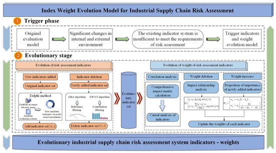
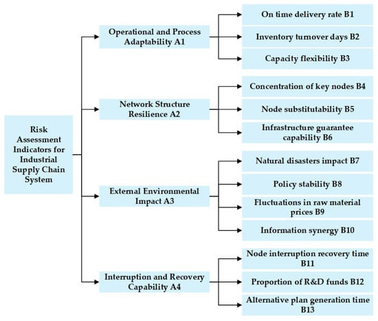
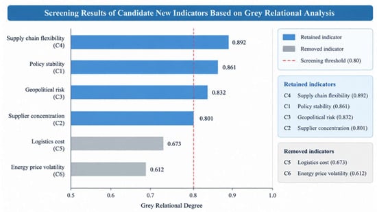
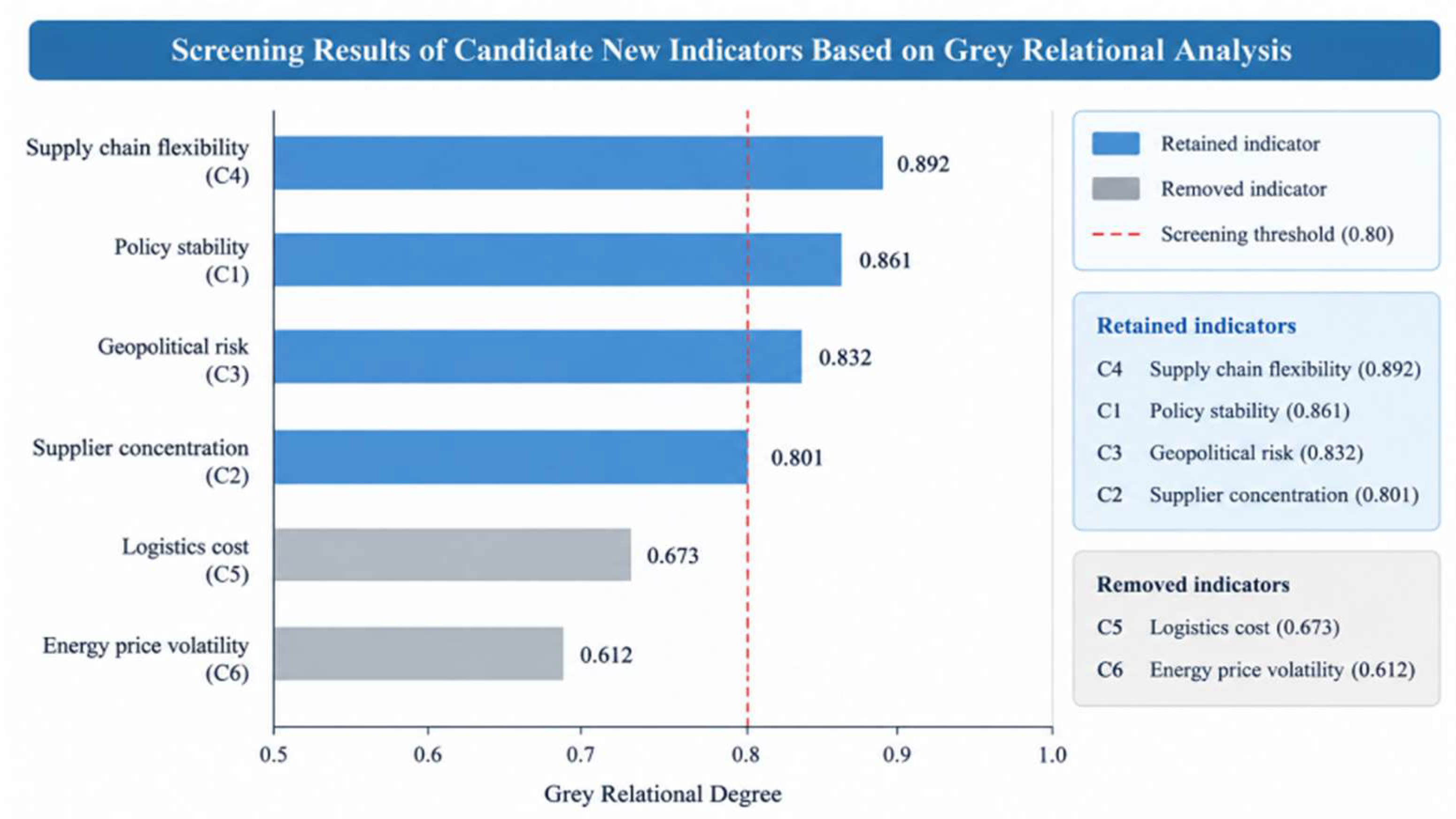
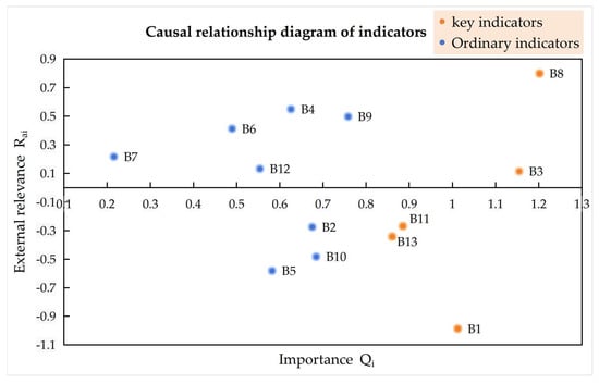
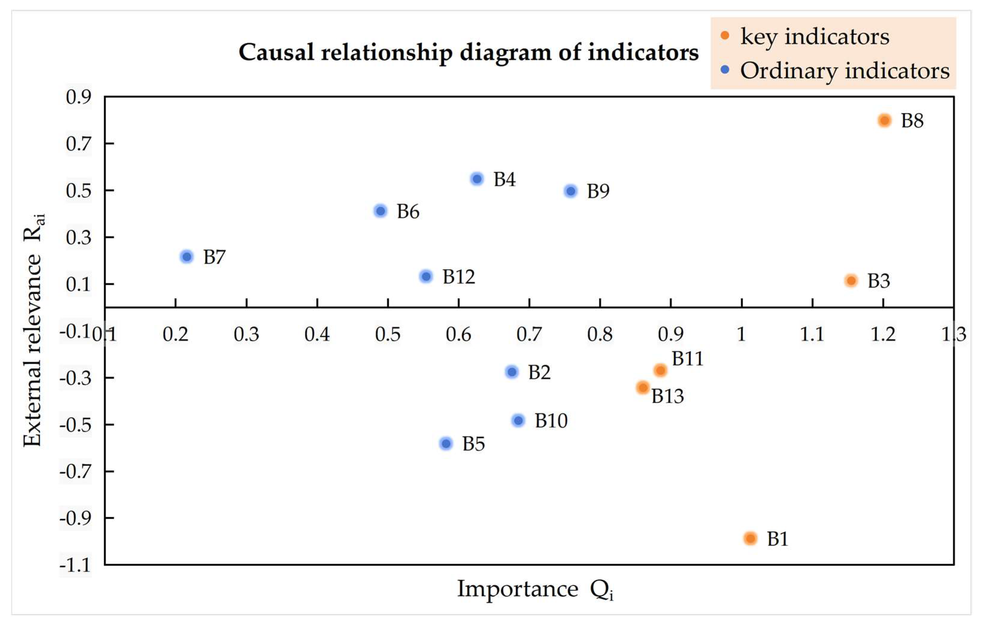
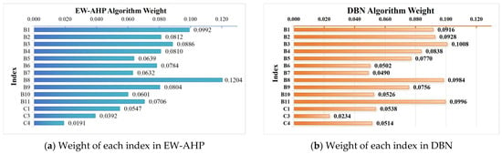
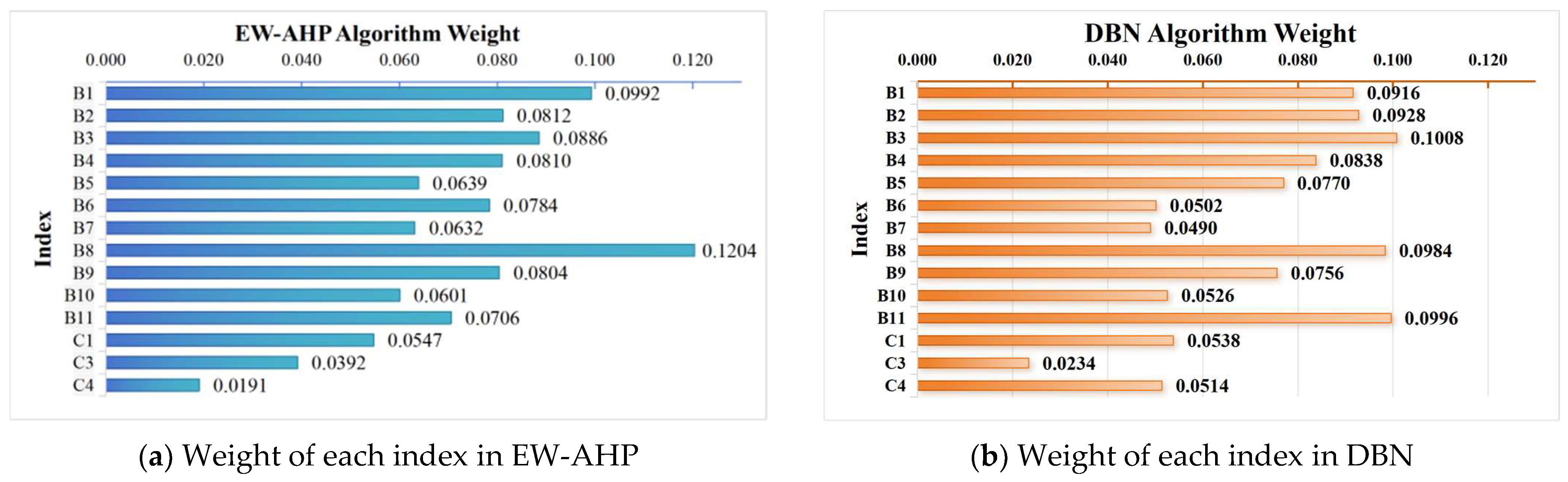
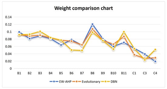
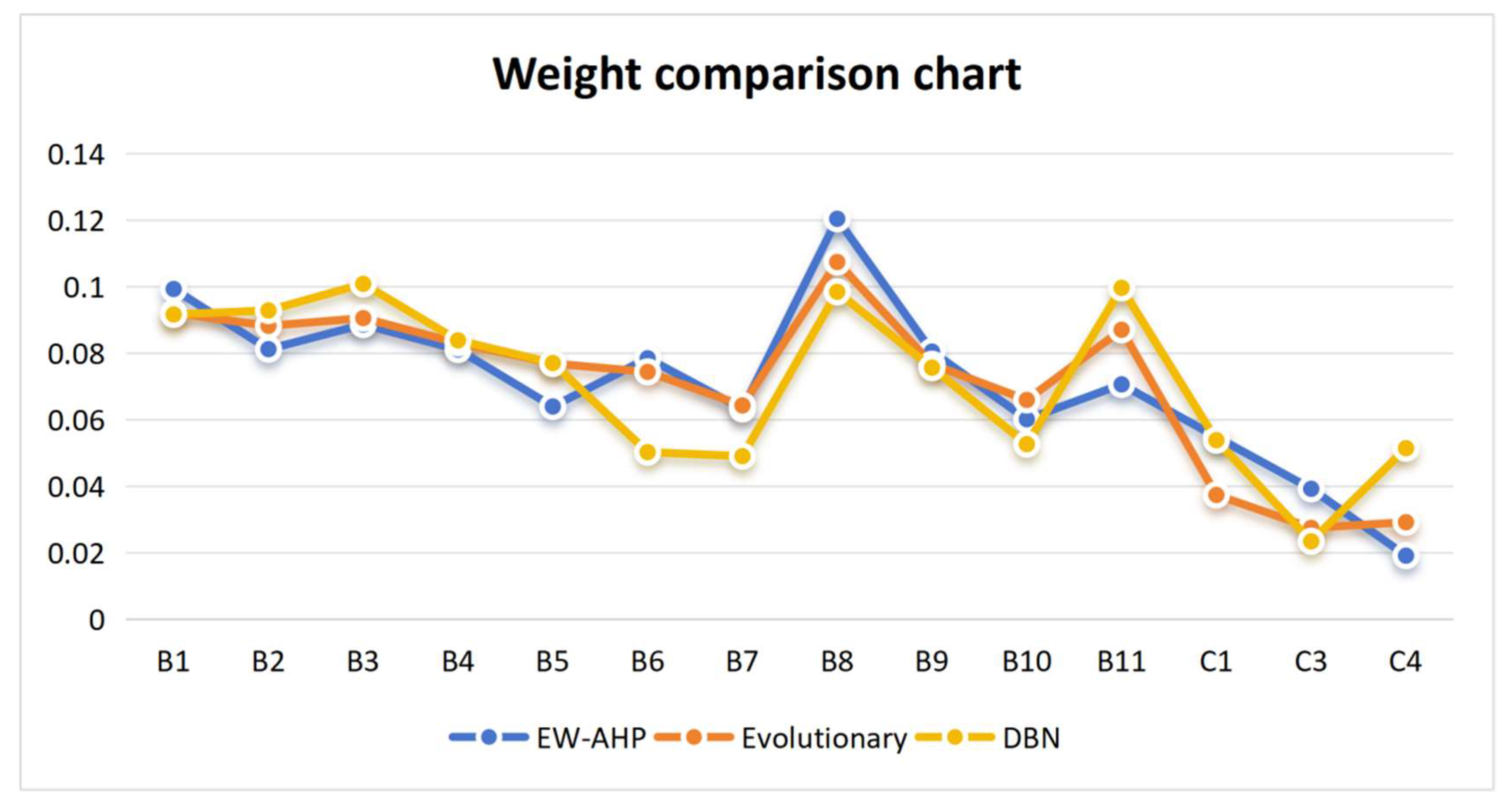
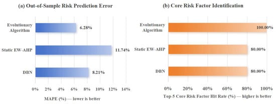
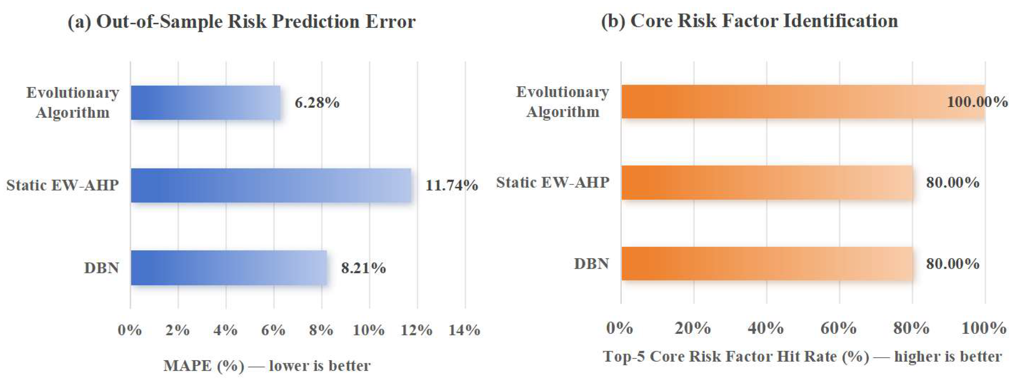

Disclaimer/Publisher’s Note: The statements, opinions and data contained in all publications are solely those of the individual author(s) and contributor(s) and not of MDPI and/or the editor(s). MDPI and/or the editor(s) disclaim responsibility for any injury to people or property resulting from any ideas, methods, instructions or products referred to in the content. |
© 2026 by the authors. Licensee MDPI, Basel, Switzerland. This article is an open access article distributed under the terms and conditions of the Creative Commons Attribution (CC BY) license.