Road Connectivity and Relative Market Accessibility in Chinese Cities: Spatial Inequality and Long-Run Decomposition

Abstract

Improved road connectivity need not produce equivalent gains in access to economic opportunities. Using modeled intercity travel times and city GDP for 278 Chinese cities during 2000–2023, we compare physical network reach with relative external market accessibility (EMA), which weights inverse road times by each origin’s external destination GDP shares. Analysis combines trends, relative and absolute inequality, spatial clustering, rank mobility, regional comparisons, and two-factor Shapley accounting. Mean intercity travel time fell by 28.7%, while relative EMA rose by 39.6%. Although relative inequality declined after 2010, absolute city-level gaps widened, spatial concentration persisted, and 202 cities occupied the same quartile at both endpoints. Nationally, the road-time component represented 97.0% of observed relative EMA growth. Northeast China reveals a sharper regional contrast: shifts in destination GDP shares offset 65.8% of favorable road-time contributions under the baseline measure, primarily through declining relative weight on other Northeast destinations. This component persists across alternative distance-decay parameters, origin weights, denominator definitions, and a targeted administrative-boundary exclusion. An exploratory comparison using city-reported growth rates to construct a comparable-price opportunity proxy also retains the negative component, although the offset magnitude and net EMA movement are sensitive to the GDP treatment and decay specification. These findings establish a transferable diagnostic sequence for regional planning: monitor connectivity and opportunities separately, assess persistent territorial disparities, and investigate destination composition alongside observed freight and economic interactions before setting intervention priorities.

1. Introduction

Accessibility describes the opportunities that a location can reach at a given travel cost. Market-potential and location-based approaches jointly consider spatial separation and destination economic mass [1,2,3]. The distinction matters for interpreting transport change: shorter journeys may enlarge a city’s reachable economic market, but the size of that gain depends on where economic activity is distributed. Recent place-based planning research argues that accessibility indicators should inform context-specific decisions rather than be read as universal prescriptions [4].

The same road network can support several legitimate but non-equivalent accessibility measures. Mean intercity travel time captures physical reach, an external GDP-weighted index incorporates where destination activity is concentrated, and a travel-time catchment identifies opportunities within a specified threshold. These measures need not rank cities similarly. We therefore evaluate RoadTA and relative external economic market accessibility (EMA) as separate core outcomes, retaining self-inclusive market coverage as a supplementary scale check. EMA represents potential exposure to the relative geography of external production; it does not directly observe sales, welfare, or the expansion of the aggregate economy. Establishing this distinction at the outset allows differences across places and years to be interpreted consistently. The practical difference is substantial: a reduction in travel time to a destination and an increase in that destination’s GDP share are distinguishable events, even when a combined index records only their net effect.

Existing evidence does not imply that better transport connections yield uniformly better economic outcomes. Faber [5] finds slower GDP growth in non-targeted peripheral counties connected to China’s National Trunk Highway System, whereas Baum-Snow et al. [6] document within-city decentralization, and Banerjee et al. [7] identify higher GDP per capita levels but not faster subsequent growth near transport networks. These results differ in spatial unit and identified outcome; jointly, they motivate analysis of where network access and potential opportunity diverge without predicting a common local growth response.

The accessibility literature likewise provides different, not interchangeable, perspectives. Historical railway and national transport studies [8,9] describe changing geographical reach; Pearl River Delta and high-speed-rail analyses [10,11,12] report mode- and region-specific patterns. Recent Chinese studies examine multimodal accessibility and population redistribution [13] or within-city constraints on facility access [14]. Neither research design directly tracks annual road-only travel times weighted by each origin’s relative external GDP. We use the Ma–Tang road-time series [15] to separate that intercity measurement question from both observed economic outcomes and intra-urban service access.

The two inputs evolve at different geographical scales. Road improvements change bilateral travel times, whereas city GDP changes the relative weights attached to external destinations. A city can become faster to reach from elsewhere without gaining comparable access to the destinations that account for the largest shares of recorded economic activity. Alternatively, the relative importance of nearby destinations may rise even where travel-time compression is limited. Annual observations help locate when such divergences emerge and whether they persist, while maintaining the same sample of origin and destination cities throughout. This temporal detail complements evidence based on selected benchmark years. It does not, however, identify the causal effect of a particular infrastructure project: our empirical task is to describe the changing joint geography of transport impedance and potential market opportunity. The use of an unchanged destination universe also separates actual indicator movement from discontinuities that would otherwise be created by adding cities to the matrix midway through the study.

Three research questions organize the analysis. RQ1: How did modeled road reach and relative external GDP-weighted accessibility change across the fixed 278-city system during 2000–2023? RQ2: Did changes in cross-city relative inequality coincide with reduced absolute gaps, weaker spatial concentration and greater rank mobility? RQ3: How much of the measured EMA change is allocated to road-time versus destination-GDP-share shifts, and do regional offsets survive alternative normalization, decay and aggregation specifications?

The empirical design proceeds across three connected scales. At the national level, annual averages establish the direction and timing of change. At the city level, dispersion, spatial association, and rank mobility reveal whether a rising mean coincides with a changing geography of relative access. At the regional level, equal-city and GDP-weighted summaries distinguish the accessibility of a typical sampled city from an average that emphasizes larger urban economies. A symmetric two-factor decomposition then allocates measured EMA change between bilateral road times and relative destination GDP shares. Keeping construction weights distinct from regional aggregation weights is essential: they answer different questions even when the underlying city-level observations are identical.

We construct annual road accessibility (RoadTA) and relative external economic market accessibility (EMA) for 278 Chinese cities in 2000–2023 using modeled prefecture-to-prefecture road times from Ma and Tang [15] and a compiled city GDP panel. We assess inequality, spatial association, ranking mobility, regional trajectories and a symmetric accounting decomposition. Self-inclusive 3-, 6- and 12-h GDP catchments are supplementary scale checks, not replacements for EMA [16,17].

The paper advances understanding on three linked levels. Conceptually, origin-specific GDP normalization isolates the relative geography of external economic opportunities; comparing it with unnormalized potential reveals the interpretive costs of each definition. Empirically, annual evidence connects national road improvement to persistent spatial inequality and identifies a large Northeast destination-share offset that is concealed by national aggregation. Operationally, the resulting diagnostic sequence directs attention toward particular origins, destinations and observed economic links when access indicators diverge.

The national–regional contrast is the paper’s central finding. Under the same external-market definition, the small positive nationwide GDP-share term coexists with a substantial negative Northeast component; Section 4.5 and Section 5.3 examine its stability under alternative specifications.

For sustainable transport appraisal, the practical lesson is to screen for disagreements among network reach, opportunity-weighted reach and territorial distribution before selecting projects. These measures can help decide where actual freight flows, service conditions and affected populations should be investigated, without implying that the present city-level indicators measure those outcomes [18].

2. Literature Review and Analytical Framework

2.1. Accessibility as the Interaction of Transport and Opportunities

Accessibility joins the distribution of opportunities to the friction of reaching them [1,2], yet methodological reviews show that alternative measures embody different welfare-relevant questions rather than interchangeable scores [3,16]. Planning applications [19,20], workplace and time-geographical approaches [17,21], and positive versus normative assessments [22] illustrate why the choice of beneficiaries, spatial scale and cost measure matters. Place-based planning [4] challenges uniform standards: identical accessibility scores can conceal different local needs. Our contribution is not another generic index but a transparent comparison of such non-equivalent measurements across the same annual city universe.

Three families of measures are relevant. A transport-only mean describes the network independently of destination economic size; inverse-cost, opportunity-weighted EMA incorporates the evolving relative geography of external GDP; and cumulative time circles describe opportunities inside explicit travel-time budgets. A city close to one large destination and a city linked to several smaller destinations may rank differently across these definitions. Thus, differences among the measures reveal precisely which aspect of access has changed; they should not be interpreted as estimation error or as a single composite sustainability score.

The supplementary time-circle comparisons follow the scale and specification concerns emphasized by Gutiérrez [23], but include local GDP without assigning an arbitrary within-city OD travel time. They do not replicate the external inverse-time EMA formula and cannot independently validate its two-factor Shapley attribution. Their value is to expose sensitivity to the opportunity set and the meaning of ‘access’ rather than to deliver an identical numerical estimate.

A distribution of modeled opportunities should also be distinguished from a normative claim about transport equity. A lower Gini coefficient indicates lower relative inequality among sampled city-level index values. Because it is normalized by the mean, it does not establish that absolute differences have diminished or that access is equal across residents, firms, or income groups. Within-city transport, logistics reliability, employment composition, and household constraints remain outside the available data. Likewise, a high national accessibility rank can coexist with substantial inequalities within a prefecture. We therefore use ‘spatial inequality’ for the descriptive distribution of city scores, reserving claims about transport justice for settings where the relevant people, needs, and outcomes can be observed [18,22].

2.2. Market Access and Economic Geography

Market-access research reaches different conclusions partly because it measures different objects. Structural work links access to bilateral trade and economic outcomes [24], and historical quasi-experiments identify valuation responses to railroad-induced market changes [25]. European accessibility and development studies [26] analyze potential reach, while Chinese high-speed-rail work links transport-cost changes to labor-market integration [27] and employment specialization [28]. These results establish the relevance of economic geography but do not imply that an origin-normalized GDP-share index measures trade, employment or causal returns to roads.

Studies of structural market access identify economic mechanisms using bilateral trade or expenditures [24,25], whereas potential-access measures use proxies such as production, population or services [26,27,28]. Our indicator belongs to the latter tradition. Origin-specific external GDP shares distinguish shifts in destination composition from uniform proportional changes in economic mass. This design makes the Northeast’s regional reweighting visible, although nominal and price-adjusted market potential answer different economic questions.

We therefore assess modeled road impedance alongside external relative GDP opportunities and use common-denominator and nominal-potential comparators to reveal how normalization changes interpretation.

2.3. Transport Infrastructure, Accessibility, and Spatial Restructuring in China

Findings on Chinese transport projects are mixed rather than uniformly equalizing. The peripheral-growth, decentralization and GDP-level results in [5,6,7] already imply heterogeneous responses; Yu et al. [29] associate motorway expansion with economic concentration, whereas Qin [30] finds disadvantages for some bypassed counties on high-speed rail lines. Taken together, the studies reject a simple ‘faster network equals broad economic catch-up’ interpretation, but concern observed outcomes and transport settings different from our normalized intercity opportunity measure.

A first unresolved question is therefore diagnostic rather than causal: can modeled city-to-city reach improve while destinations important to a city’s relative economic opportunity shift elsewhere? Annual bilateral inputs and a constant destination universe make that question observable in the EMA accounting system. Subsequent verification against real transactions, industrial linkages and freight would be needed to assess mechanisms.

Measurement matters for regional cohesion. European work shows that road investments, spatial spillovers and convergence conclusions depend on the chosen accessibility definition [31,32,33]. Chinese transport studies similarly report different patterns across rail, road and multimodal settings [8,9,10,11,12,34,35]. Cabello et al. [36] emphasize the distribution of accessibility benefits in regional transport plans, while Jiao et al. [37] examine accessibility and economic growth in China. Together, these studies support reporting both accessibility levels and city rankings rather than inferring uniform gains from a national average.

Ma and Tang [15] provide annual modeled bilateral road times, allowing a fixed-city comparison with external GDP opportunities. In contrast, Lyu and Zhao [13] examine multimodal accessibility and population redistribution at five benchmark years, and Wang et al. [14] investigate urban form and local facility access. We track annual road-only origin–destination impedance weighted by each origin’s relative external GDP composition, then ask how spatial inequality and destination-specific regional offsets evolve together.

Condeço-Melhorado et al. [38] offer the closest decomposition antecedent, analyzing Spanish accessibility with decennial networks, population-weighted potential and a symmetric multiplicative index approach. Our contribution differs in annual temporal resolution, the exclusion of each origin’s own opportunity, origin-normalized GDP weights, and exact additive two-factor accounting. These design choices uncover a substantive result: apparently minor national destination-share contributions conceal a large Northeast-specific counterweight to road-time improvement. The estimation tools are established; the new contribution is the regional pattern and its measured sensitivity.

2.4. Research Gap and Analytical Positioning

The unresolved question is how a national improvement in road reach can coexist with weaker gains in particular regions’ relative access to economic activity. The annual fixed-city network, explicit destination weights and origin-level counterfactual accounting allow us to locate this contrast. Adding inequality, spatial association and rank mobility reveals whether the aggregate advance changes the underlying territorial hierarchy. The Northeast offers a clear test of the framework’s value, particularly when alternative GDP and distance-decay assumptions are applied.

Beyond its China-specific result, the contribution is a transferable diagnostic: identify network–opportunity divergence, locate the destinations behind the offset, and determine which real transport and economic interactions should be investigated. Its sensitivity to alternative measurement choices is assessed below.

We examine three non-causal expectations corresponding to the research questions. First, shorter modeled road times should improve network reach but may not produce proportionate relative-EMA gains. Second, an improving EMA mean need not eliminate absolute gaps, spatial clustering or rank persistence. Third, an aggregate GDP-share contribution near zero may conceal larger regional terms of opposite sign. These expectations are evaluated in Section 4, with the constraints on interpretation discussed in Section 5.

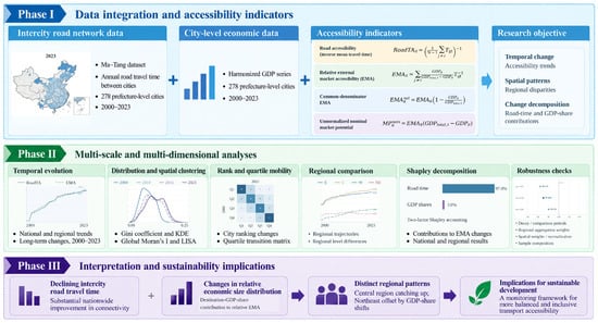
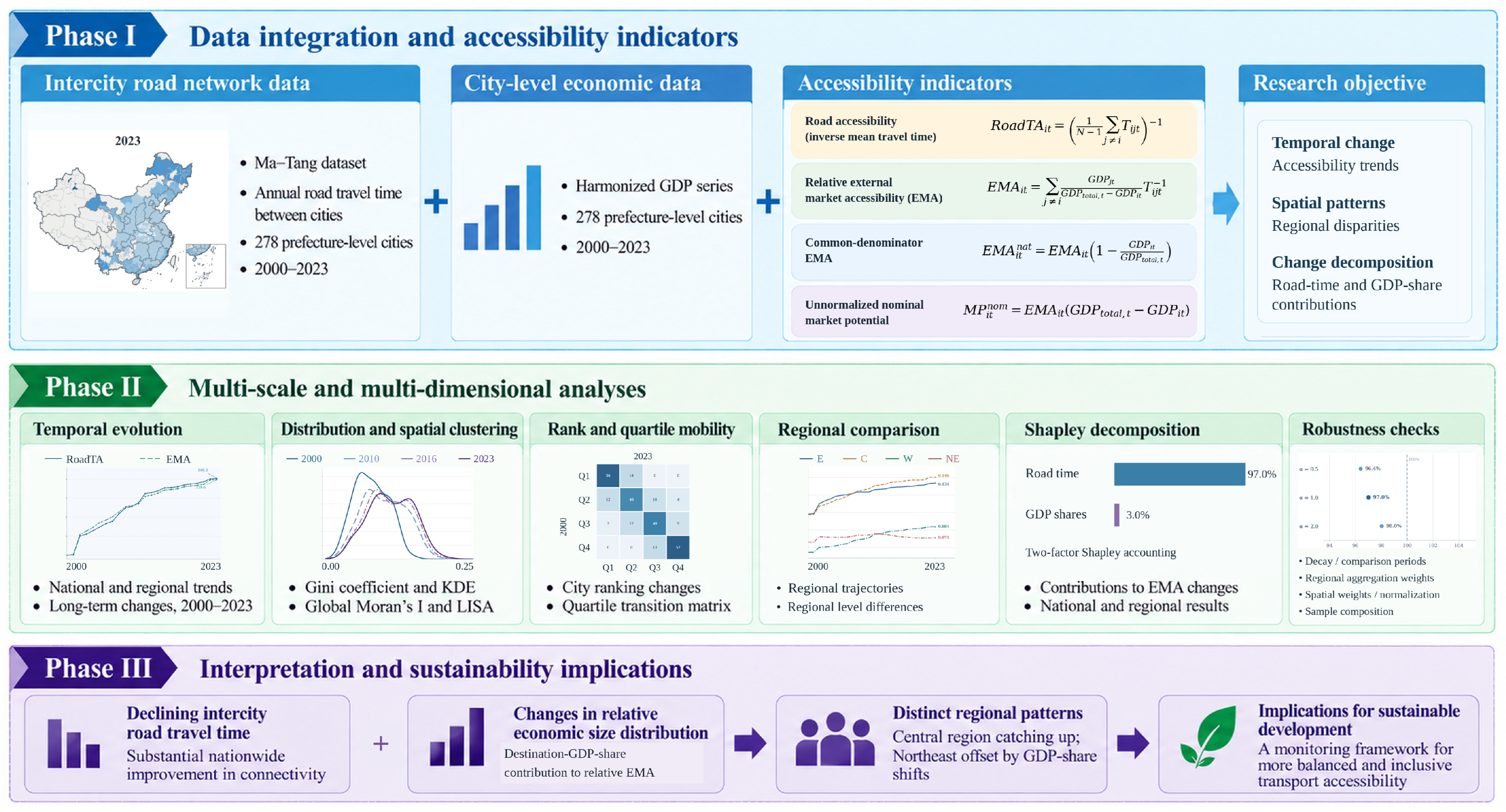
Figure 1 brings together the four complementary indicators, their annual and spatial comparisons, and the regional accounting steps used to identify actionable questions for transport and economic planning.

Figure 1. Analytical framework of the study: complementary measures of road access and economic opportunities, distributional analyses, and regional decomposition.

3. Materials and Methods

3.1. Study Area and Data Sources

The fixed research universe comprises 278 city units matched to the 279 nodes of Ma–Tang v2.0, excluding the former Laiwu unit, for 2000–2023. The 278 units are distributed across the East (84), Central (80), West (82) and Northeast (32). Coverage is uneven: Tibet has no sampled unit, and Guizhou and Qinghai contribute two and one, respectively; the detailed provincial pattern is presented with the regional evidence. As omitted cities are absent from both origin and destination sets, the resulting statistics describe this fixed system rather than all Chinese jurisdictions. For context, the National Bureau of Statistics (NBS) reported 297 prefecture-level-and-above cities in 2023; the ratio 278/297 is only a numerical comparison, not a verified city-by-city coverage rate across the full study period.

The former Laiwu node is excluded from all OD matrices; Jinan remains as recorded in the NBS-derived GDP series, without manually adding or subtracting historical Laiwu output. For visualization, we use a fixed GS(2024)0650 administrative display layer, which depicts the former Laiwu area within Jinan. Known changes affecting Chaohu and Jianyang motivate a joint exclusion of six affected origin/destination nodes; the Northeast result remains similar. These checks do not reconstruct every historical city boundary.

The Ma–Tang v2.0 road-only file (pref_pair/time_cost_prefecture_pair_road.csv), together with cityinfo.csv, provides modeled annual shortest-road-time OD data; we retain 2000–2023 and match administrative codes before constructing symmetric OD matrices. The authors assembled the GDP worksheet from the National Bureau of Statistics (NBS) National Data platform (https://data.stats.gov.cn/). The analysis uses the original-data sheet’s current-price total-GDP field (RMB 10,000) for all 6672 study city-years, without substituting imputed-sheet values or sums of industrial value added. Official historical revisions may be reflected in this archived file; no independently harmonized, constant-area or single-vintage GDP panel is claimed. Growth rates from the same workbook permit a separate 275-city price-treatment sensitivity check, not an independently verified local GDP deflator. The archived OD and GDP snapshots, city crosswalk and analysis scripts determine the replicable input set.

For statistical programming, ChatGPT (GPT-5.6 model, OpenAI, San Francisco, CA, USA) assisted with drafting and debugging portions of the analysis scripts; authors reviewed the code and checked principal calculations against archived inputs. Product and use details are stated in the Acknowledgments.

The road-time input, the core and complementary accessibility measures, and the spatial weighting scheme are defined with their respective units in Table 1.

Table 1. Core data and operational definitions.

Measure	Symbol	Definition	Unit/Scope
Road travel time	Tijt	Modeled shortest road time from i to j	hours
Road accessibility	RoadTA	Inverse mean time to other 277 cities	h−1
External market accessibility	EMA	GDP-share-weighted inverse travel time, origin excluded	h−1
EMA (common base)	EMAnat,it	External GDP-time numerator/total study-city GDP	h−1
Nominal market potential	MPnom,it	External GDP-time numerator without GDP normalization	RMB 100 million × h−1
Self-inclusive coverage	TC(τ)	Share of sample GDP reachable within τ hours, including home GDP	%
Spatial weights	W	Row-standardized nearest-neighbor matrix (k = 5; k = 8 check)	dimensionless

3.2. Road Accessibility

A simple road accessibility measure describes each city’s position in the national road network independently of destination market size. Let T_ijt denote the shortest road travel time between origin city i and destination city j in year t, and let N denote the number of sample cities. Road accessibility is defined as the inverse of mean travel time to all other cities, as shown in Equation (1):

$${\mathrm{RoadTA}}_{\mathit{it}}={\left[{\displaystyle \frac{1}{N-1}}{\displaystyle \sum _{j\ne i}}{T}_{\mathit{ijt}}\right]}^{-1}$$

(1)

RoadTA gives identical weight to every external destination when averaging travel times and then takes the reciprocal of that average. It summarizes physical reach within the sampled urban system rather than destination market size. Two cities with similar mean travel times may differ in the distribution of nearby and distant connections or in surrounding economic mass. A peripheral city can also record a large proportional improvement while remaining distant in hours. Indexed changes and unindexed levels are therefore reported together. The subsequent comparison with EMA retains these distinctions rather than treating the indicators as identical formulas with different weights.

A larger RoadTA indicates a lower mean modeled travel time to the other study cities. Selected figures normalize the sample-wide annual mean of city-level RoadTA to 2000 = 100; the calculations retain each city’s untransformed value. This mean of reciprocal city averages is distinct from the reciprocal of the pooled mean travel time, another consequence of nonlinear aggregation. Both are descriptive summaries of modeled links, not observed door-to-door travel or generalized freight cost.

3.3. External Economic Market Accessibility

The core indicator is external economic market accessibility (EMA). For origin city i and year t, each destination j ≠ i receives a GDP weight normalized over the other 277 sample cities (Equation (2)):

$${\omega }_{\mathit{ijt}}={\displaystyle \frac{{\mathrm{GDP}}_{\mathit{jt}}}{{\sum }_{k\ne i}{\mathrm{GDP}}_{\mathit{kt}}}}$$

(2)

EMA is then calculated as the GDP-share-weighted inverse travel time (Equation (3)):

$${\mathrm{EMA}}_{\mathit{it}}={\displaystyle \sum _{j\ne i}}{\omega }_{\mathit{ijt}}{T}_{\mathit{ijt}}^{-1}$$

(3)

The difference between the two baseline indices is not a pure GDP-weighting contrast. Define U_it as the equally weighted mean of inverse travel times T_ijt⁻¹ to the other N−1 destinations. By comparison, RoadTA_it is the reciprocal of their mean travel time. For positive times, convexity implies U_it ≥ RoadTA_it, with equality only when all external travel times are identical. The exact level difference is expressed in Equation (4):

EMA_it − RoadTA_it = (EMA_it − U_it) + (U_it − RoadTA_it)

(4)

The first term compares GDP weighting with uniform weighting of inverse times; the second captures the aggregation difference. This diagnostic does not replace either baseline indicator. GDP-share contributions to changes in EMA are identified arithmetically within the fixed EMA function in Section 3.6, not from the RoadTA–EMA gap.

Two same-source comparators clarify the interpretation of the baseline EMA. Let GDP_total,t denote the sum of GDP across all 278 study cities in year t. First, a common-denominator indicator uses the full-sample GDP total rather than the sum of external GDP for each origin. It retains exactly the same external destinations and bilateral road times as the baseline, so this is a denominator check rather than a test of adding the home market, as shown in Equation (5):

$$\begin{array}{l}{\mathit{EMA}}_{\mathit{it}}^C={\displaystyle \frac{{\displaystyle {\sum }_{j\ne i}}GD{P}_{\mathit{jt}}/T_{\mathit{ijt}}}{{\mathit{GDP}}_{\mathrm{total},t}}}\\ {\mathit{EMA}}_{\mathit{it}}^C={\mathit{EMA}}_{\mathit{it}}\left(1-{\displaystyle \frac{{\mathit{GDP}}_{\mathit{it}}}{{\mathit{GDP}}_{\mathrm{total},t}}}\right)\end{array}$$

(5)

Equation (5) shows that the common national GDP denominator scales the origin-normalized indicator by the share of sample GDP located outside the origin. It therefore introduces the own-city share into comparisons despite leaving the underlying external opportunities unchanged. Second, to retain the total contemporaneous GDP mass without normalized destination shares, we define nominal market potential in Equation (6):

$$\begin{array}{l} M{P}_{\mathit{it}}^N={\displaystyle \sum _{j\ne i}}{\displaystyle \frac{{\mathit{GDP}}_{\mathit{jt}}}{T_{\mathit{ijt}}}}\\ M{P}_{\mathit{it}}^N={\mathit{EMA}}_{\mathit{it}}\left({\mathit{GDP}}_{\mathrm{total},t}-{\mathit{GDP}}_{\mathit{it}}\right)\end{array}$$

(6)

Equation (6) has GDP-per-hour units, while both normalized EMA indicators have inverse-hour units. Because it incorporates the scale of current-price GDP, the nominal comparator should not be interpreted as inflation-adjusted market growth. These definitions establish the normalization checks; the central geographic and Shapley analyses retain the origin-specific baseline EMA.

RoadTA captures average modeled network reach; EMA measures GDP-share-weighted inverse road times; the common-denominator variant uses total study-city GDP in the denominator without adding home-city opportunity; and nominal potential restores economic mass. Self-inclusive 3-, 6- and 12-h catchments answer a distinct threshold question, with benchmark coverage summarized in Table A1. To probe price sensitivity, we additionally chain each city’s reported annual GDP growth rates from its 2000 nominal GDP and construct a comparable-growth opportunity proxy for the 275 cities with complete 2001–2023 rates. Both nominal and growth-chained decompositions are recomputed on that identical 275-city origin/destination universe, so sample exclusion and GDP treatment can be distinguished. This is a sensitivity analysis based on reported growth rates, not a verified city-specific deflator series; historical revisions may affect the implied price factors.

3.4. Distributional and Spatial Diagnostics

The temporal evolution of accessibility is examined using annual national means over 2000–2023. Geographic maps and density snapshots use 2000, 2010, 2016, and 2023, while the tabular benchmark summaries additionally include 2020. The Gini coefficient summarizes relative cross-city inequality: it equals the mean absolute difference across all ordered city pairs, including self-pairs, divided by twice the mean EMA. Consequently, a lower Gini need not imply smaller absolute differences. Kernel density estimates describe the distribution in its original inverse-hour units rather than after normalization by the annual mean. Spatial association is assessed separately from both distributional measures.

Spatial statistics use Ma–Tang cityinfo.csv coordinates and great-circle (haversine) distances. Directed k-nearest-neighbor links are not symmetrized; row weights sum to one. We use k = 5 as the baseline; Table A2 provides the benchmark comparison with k = 8. Annual Global Moran’s I [39] is accompanied by benchmark 499-permutation pseudo-p values. LISA [40] classifications use 999 conditional randomizations for mapped years and nominal p < 0.05. The reported change in Moran’s I describes the strength of spatial association at the two endpoints; the manuscript does not present a formal cross-year difference test.

3.5. City-Rank Mobility and Regional Comparison

We compare 2000 and 2023 city rankings using Spearman correlations, top-20 retention, and absolute rank displacement for RoadTA and EMA. For EMA quartile mobility, each endpoint is ranked separately and divided into four near-equal groups; the boundaries are rank-based within each year, not fixed numerical EMA values. The transition matrix therefore describes endpoint repositioning. For the most extreme upward and downward movers, we also compare initial mean road time and modeled time to the nearest of the 20 cities with the highest GDP in 2000, excluding an origin from its own candidate destinations. Alternative top-10, top-15 and top-30 hub definitions provide a sensitivity check.

Four macro-regions (East, Central, West and Northeast) follow the conventional provincial grouping. Eastern China contains Beijing, Tianjin, Hebei, Shanghai, Jiangsu, Zhejiang, Fujian, Shandong, Guangdong and Hainan; Central China includes Shanxi, Anhui, Jiangxi, Henan, Hubei and Hunan; the Northeast includes Liaoning, Jilin and Heilongjiang; and the remaining sample provinces form the West. The primary regional EMA statistic weights each sample city equally. As an additional aggregation check, 2023 regional EMA is also averaged using origin-city GDP weights from 2023 and, separately, from the fixed year 2000. These are alternative summaries of the same cities, not revised city-level EMA formulas (Section 4.4).

3.6. Symmetric Decomposition of EMA Change

We apply the symmetric two-factor Shapley accounting principle described by Shorrocks [41]; Condeço-Melhorado et al. [38] use a related but distinct accessibility-decomposition approach. Define A(T,M) as the equal-origin-weighted mean of baseline EMA evaluated under road-time matrix T and relative destination-GDP-share array M. Equation (7) states the endpoint difference for 2000 and 2023. The four counterfactual combinations are reconstructed from bilateral OD data and matched annual GDP shares; subperiod comparisons provide an additional check of national attribution.

ΔA = A(T₂₀₂₃, M₂₀₂₃) − A(T₂₀₀₀, M₂₀₀₀)

(7)

A one-directional decomposition depends on the order in which the two factors are updated. For two factors, the symmetric Shapley principle averages each factor’s marginal contribution over both possible update orders, yielding an exact additive identity. We calculate the counterfactuals at the origin-city level and then take equal-origin means for national and regional results. The GDP-share contribution includes origin-specific renormalization, not simply the change in a national GDP fraction. To locate the Northeast offset more precisely, we attribute each bilateral GDP-share contribution to the destination’s macro-region before aggregation. These accounting allocations must not be mistaken for observed trade, migration or investment mechanisms.

Equation (8) defines the contribution of the road-time matrix as the mean of two time-updating paths, once with GDP shares fixed at the initial year and once at the final year.

$$\Delta A^N={\displaystyle \frac{1}{2}}\left\{\left[A\left(T_{23},M_{00}\right)-A\left(T_{00},M_{00}\right)\right]+\left[A\left(T_{23},M_{23}\right)-A\left(T_{00},M_{23}\right)\right]\right\}$$

(8)

Equation (9) gives the corresponding GDP-share contribution, holding each endpoint road-time matrix fixed in turn.

$$\Delta A^M={\displaystyle \frac{1}{2}}\left\{\left[A\left(T_{00},M_{23}\right)-A\left(T_{00},M_{00}\right)\right]+\left[A\left(T_{23},M_{23}\right)-A\left(T_{23},M_{00}\right)\right]\right\}$$

(9)

By construction, the road-time and GDP-share terms sum exactly to the change in the selected relative EMA measure. Reported shares depend on the index normalization, the decay exponent, and the comparison years. A road-time share exceeding 100% means that the GDP-share component offsets part of a positive net change. The allocation describes the index’s arithmetic composition; no investment-treatment effect is estimated.

We reconstruct the counterfactuals for inverse-time decay exponents α = 0.5, 1 and 2, with either external-origin or common GDP denominators, and aggregate Northeast origins using city-equal or fixed 2000/2023 GDP weights. The origin weights are held fixed across counterfactual combinations. The same calculation is repeated on the matched 275-city nominal and growth-chained GDP sample, and after excluding six identified administrative-adjustment cities. The resulting regional growth and Northeast decomposition comparisons are assembled in Table A3. Contributions have units of hours raised to the power −α and must not be compared as absolute levels across exponents; the offset share is the magnitude of the negative GDP-share contribution relative to the positive road-time term.

3.7. Self-Inclusive Travel-Time Catchments

For the complementary scale check, we calculate self-inclusive GDP coverage within τ ∈ {3, 6, 12} modeled road-travel hours. For an origin city, this is the share of total sample GDP located either in the origin itself or in destinations reachable within the threshold. Own-city GDP enters without assigning an artificial intra-city travel time. This convention makes the threshold metric well-defined for self-inclusion, but its scope and units differ from external inverse-time EMA. The threshold-based perspective complements continuous impedance weighting [17,23]. Equation (10) defines the time-circle indicator.

$${\mathrm{TC}}_{\mathit{it}}\left(\tau \right)={\displaystyle \frac{{\mathrm{GDP}}_{\mathit{it}}+{\displaystyle {\sum }_{j\ne i}}{\mathrm{GDP}}_{\mathit{jt}}\hspace{0.17em}\mathbf{1}\left(T_{\mathit{ijt}}\le \tau \right)}{{\displaystyle {\sum }_k}{\mathrm{GDP}}_{\mathit{kt}}}}$$

(10)

Time-circle coverage checks how conclusions differ when local GDP is included and access is defined by a threshold rather than a continuous impedance weight. Large origins may have high short-range coverage because they contain substantial economic activity themselves, while smaller origins may benefit from proximity to external centers. A destination crossing a three-hour boundary changes the cumulative indicator discontinuously. We therefore compare patterns and ranks across measures, not their levels or implied welfare effects.

4. Results

4.1. Long-Run Improvement and Decelerating Gains

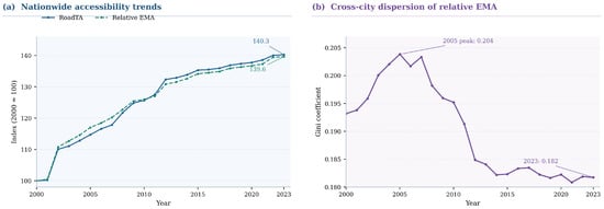
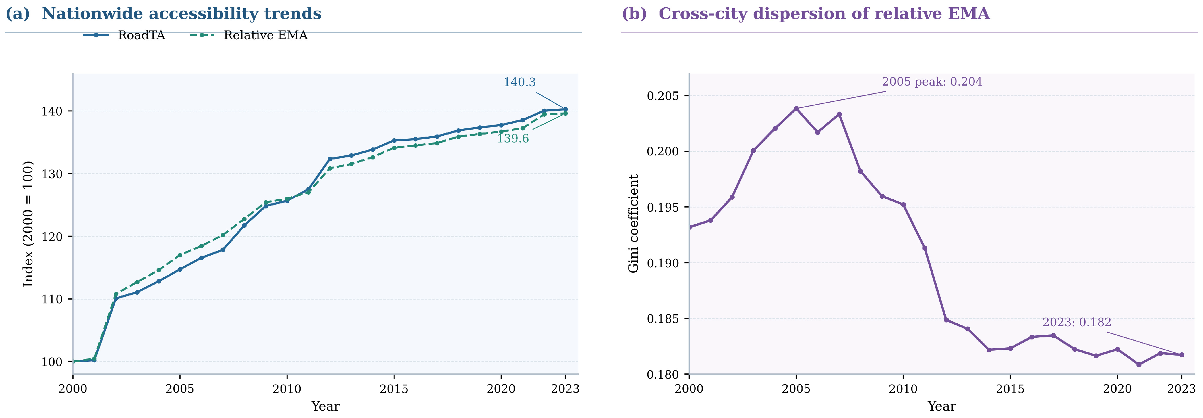
Figure 2a and Table 2 document a large improvement in modeled intercity road reach within the fixed 278-city system. Mean bilateral road travel time fell from 19.57 h in 2000 to 13.96 h in 2023 (−28.7%). With national means indexed to 2000 = 100, RoadTA reached 140.3 and relative EMA 139.6 in 2023. The indexed trajectories provide parallel descriptions of transport-only and opportunity-weighted access across the fixed 278-city panel.

Figure 2. National trends in road accessibility, relative market accessibility, and relative cross-city inequality, 2000–2023.

Table 2. National benchmark-year accessibility, inequality, and spatial autocorrelation.

Year	Mean Travel Time (h)	RoadTA Index	EMA Index	EMA Gini	Moran’s I
2000	19.57	100.0	100.0	0.193	0.858
2010	15.66	125.7	126.0	0.195	0.909
2020	14.21	137.7	136.7	0.182	0.908
2023	13.96	140.3	139.6	0.182	0.914

Note: All benchmark Moran’s I values have permutation pseudo-p = 0.002 (499 permutations).

The roughly 5.6-h reduction concerns the mean of modeled intercity pairs, not a representative observed freight or passenger journey. The national RoadTA and EMA indices follow similar upward paths even though the former weights destinations equally and the latter weights them by external GDP shares. Figure 2 also shows a slower rate of increase after the first decade. These aggregate patterns provide a baseline for examining cross-city dispersion and regional deviations in the subsequent subsections. The distinction between a national change in hours and a national percentage change in an inverse-time index also matters: inversion is nonlinear, so the two transformations need not display precisely the same growth rate.

The indexed series conceal city-level differences, and their proximity does not isolate GDP weighting because RoadTA and EMA also differ in the order of inversion and averaging. A same-input diagnostic illustrates the distinction: the national mean of equally weighted inverse travel times is 0.074991 in 2000 and 0.107760 in 2023, compared with RoadTA means of 0.054101 and 0.075890, respectively. The corresponding EMA means are 0.081478 and 0.113750. Thus, the level difference between RoadTA and EMA combines a reciprocal-aggregation component and a destination-GDP-weighting component. Attribution of EMA change to GDP shares relies on the within-EMA counterfactual decomposition in Section 4.5, not on the separation between the indexed lines.

RoadTA increased by 25.7% and relative EMA by 26.0% during 2000–2010, with smaller proportional increments thereafter. In a same-source denominator check, replacing the external-GDP denominator with the common sample-GDP denominator changes the 2000–2023 national EMA growth rate from 39.61% to 39.62%.

The near identity in national growth under the two normalized definitions does not imply that the conversion factor is constant across cities. It varies with the GDP share of each origin, so the common-denominator index is most distinct for relatively large urban economies. Nominal market potential, by contrast, also scales with the substantial increase in current-price GDP during the period. It is retained as a unit and normalization comparator, not interpreted as a price-adjusted measure of growth in reachable economic activity.

4.2. Relative Inequality and Persistent Spatial Clustering

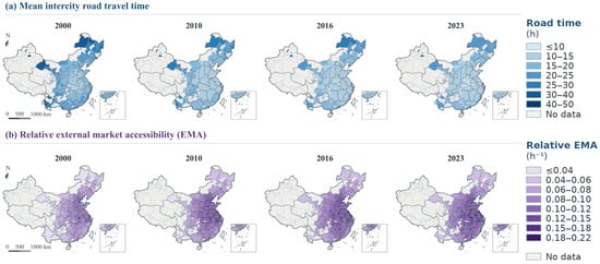
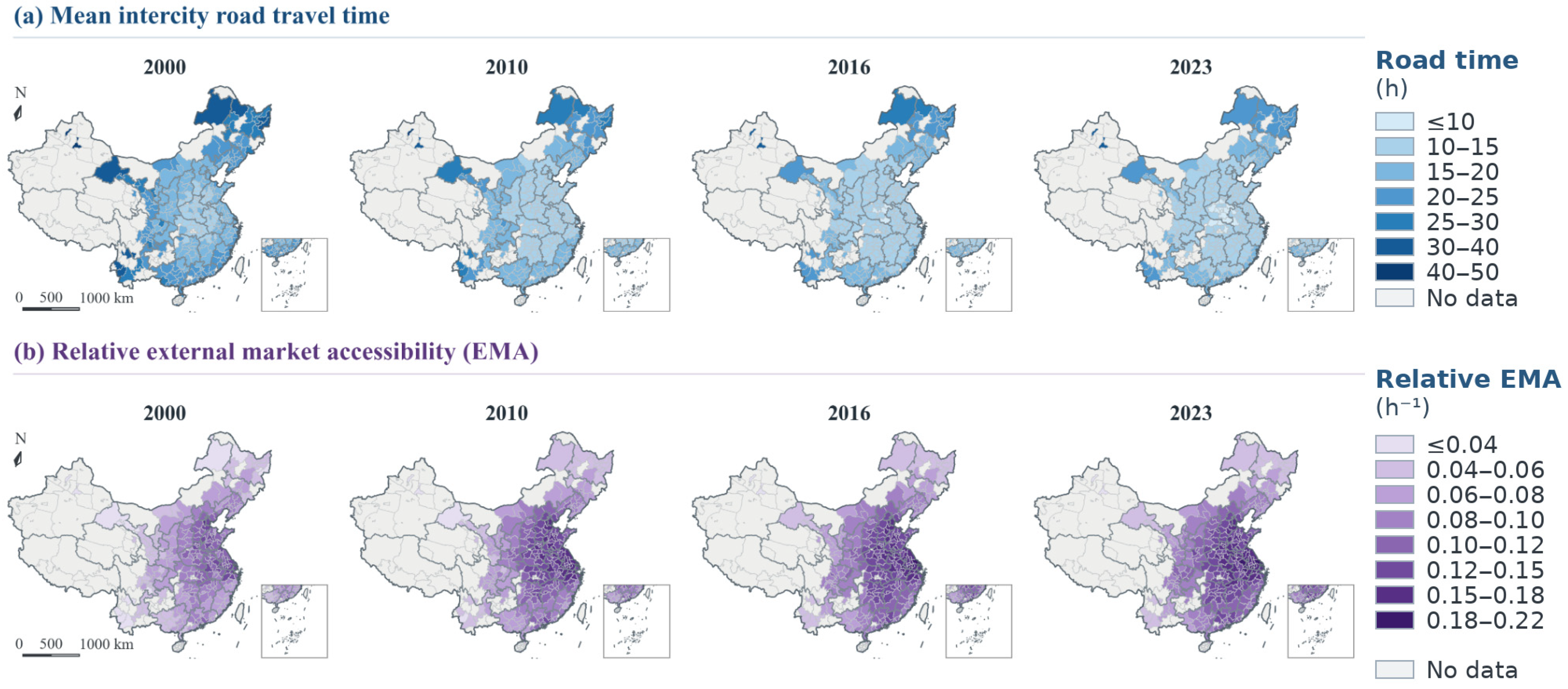
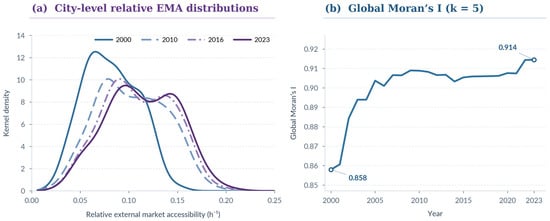
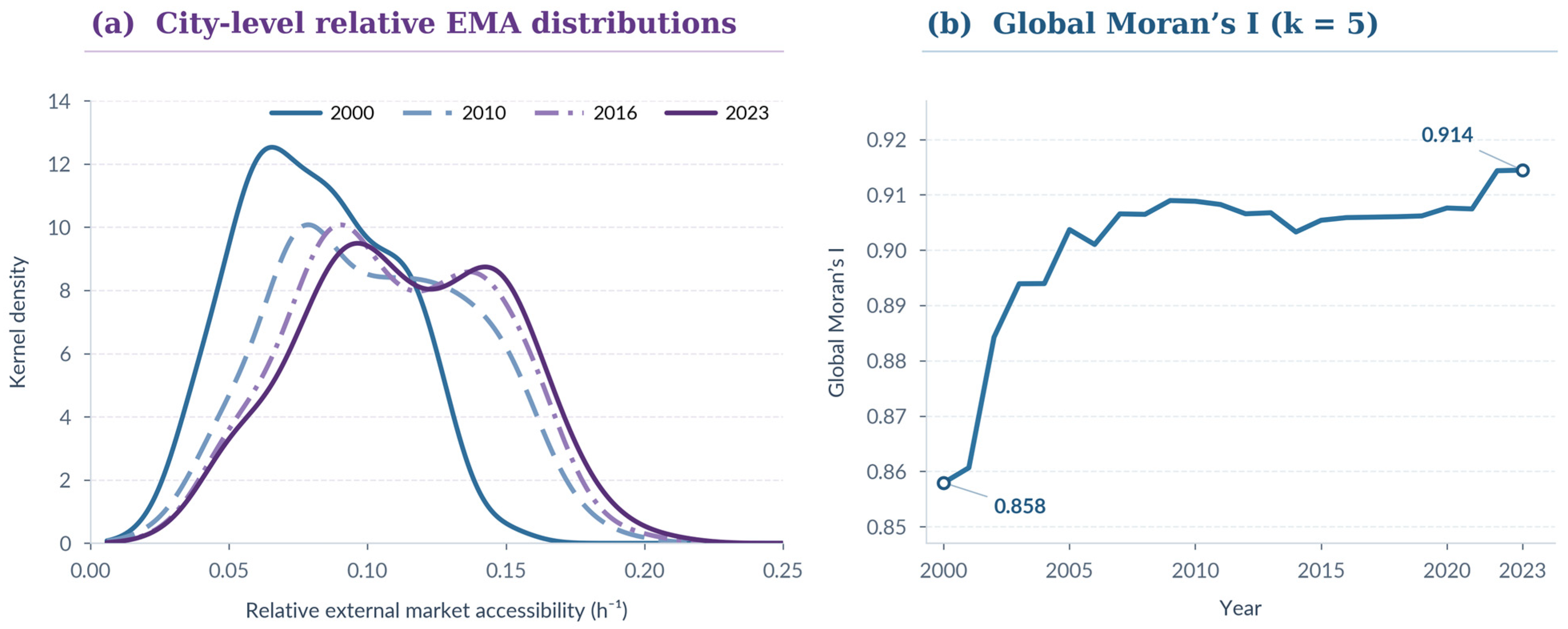
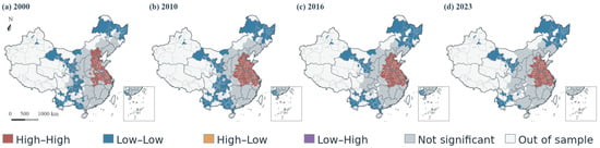
Relative inequality in city-level EMA declined during the later part of the study period, but not continuously from its start. The annual Gini coefficient rose from 0.193 in 2000 to a peak of approximately 0.204 in 2005, before declining to 0.195 in 2010 and 0.182 in 2023 (Figure 2b). Figure 3 maps mean intercity road travel time and relative EMA in 2000, 2010, 2016, and 2023 under indicator-specific common class intervals; Figure 4 combines density snapshots for those years with annual global spatial association. These displays distinguish mean-normalized inequality, the distribution of index levels, and their spatial arrangement.

Figure 3. Spatial distribution of mean intercity road travel time and relative external market accessibility in Chinese cities, 2000, 2010, 2016, and 2023. Note: Class breaks are fixed across mapped years. Administrative boundary layer: China Standard Administrative Division Data, GS(2024)0650; gray denotes areas outside the matched sample.

Figure 4. Distributional evolution and spatial autocorrelation of relative external market accessibility, 2000–2023. Note: The KDE uses Scott’s bandwidth.

The distributional profiles in Figure 4a complement the Gini statistics because they retain the original scale of EMA. A direct check of the same 278-city panel shows that the mean absolute difference across all ordered city pairs rose from 0.031480 in 2000 to 0.041343 in 2023, in inverse-hour units, while mean EMA increased from 0.081478 to 0.113750. The decline in the Gini therefore describes smaller differences relative to the rising mean, not smaller absolute gaps between cities. The 2023 maps still show pronounced high-accessibility concentrations. Their persistence is consistent with lower relative inequality and does not imply broad territorial convergence.

The early-period rise and subsequent decline in the Gini provide context for the benchmark density curves. The two summaries answer different questions: the Gini scales differences by the annual mean, whereas the density plots display the frequency of EMA levels in their original units. The four-year maps locate those levels geographically. The remaining question is whether spatial association changed alongside the later reduction in relative inequality.

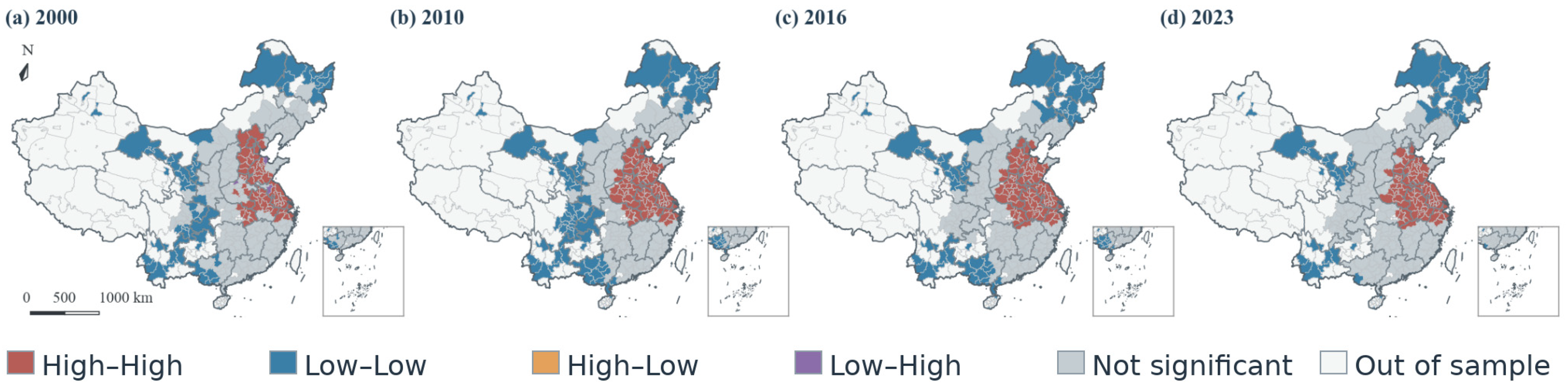
Figure 3 shows that the highest EMA values remain concentrated in contiguous portions of the national study area. Figure 4 and Figure 5 provide complementary spatial diagnostics: Global Moran’s I summarizes neighborhood association, while local indicators classify particular configurations. Taken together, these results show that lower relative inequality after 2010 coexists with persistent geographic structure. Rank persistence is assessed separately in Section 4.3.

Figure 5. Local spatial clustering of relative external market accessibility in Chinese cities, 2000, 2010, 2016, and 2023. Note: Administrative boundary layer: GS(2024)0650. Clusters use uncorrected p < 0.05; nonsignificant sampled cities are distinguished from areas outside the sample.

Global Moran’s I increased from 0.858 in 2000 to 0.914 in 2023 (Figure 4b), indicating strong positive spatial association at both endpoints under the stated five-nearest-neighbor matrix. The nominal LISA classifications in Figure 5 show local configurations in 2000, 2010, 2016, and 2023. High–High and Low–Low concentrations remain visible across the mapped snapshots; the archived endpoint High–High counts are 66 in 2000 and 77 in 2023. The classification depends on unadjusted local permutation tests, so the change in counts is descriptive and should not be portrayed as a multiplicity-corrected structural shift.

The permutation tests assess association within each year’s spatial configuration, not the significance of the difference in Moran’s I between years. Local High–High and Low–Low classifications depend on the chosen neighbors and unadjusted local tests; the reported counts should therefore be read as descriptive assignments. For k = 8, Moran’s I remains positive at both endpoints (0.8142 in 2000 and 0.8801 in 2023), providing a wider-neighborhood comparison without a formal test of the difference.

4.3. Persistent Hierarchy and Selective Rank Repositioning

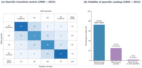
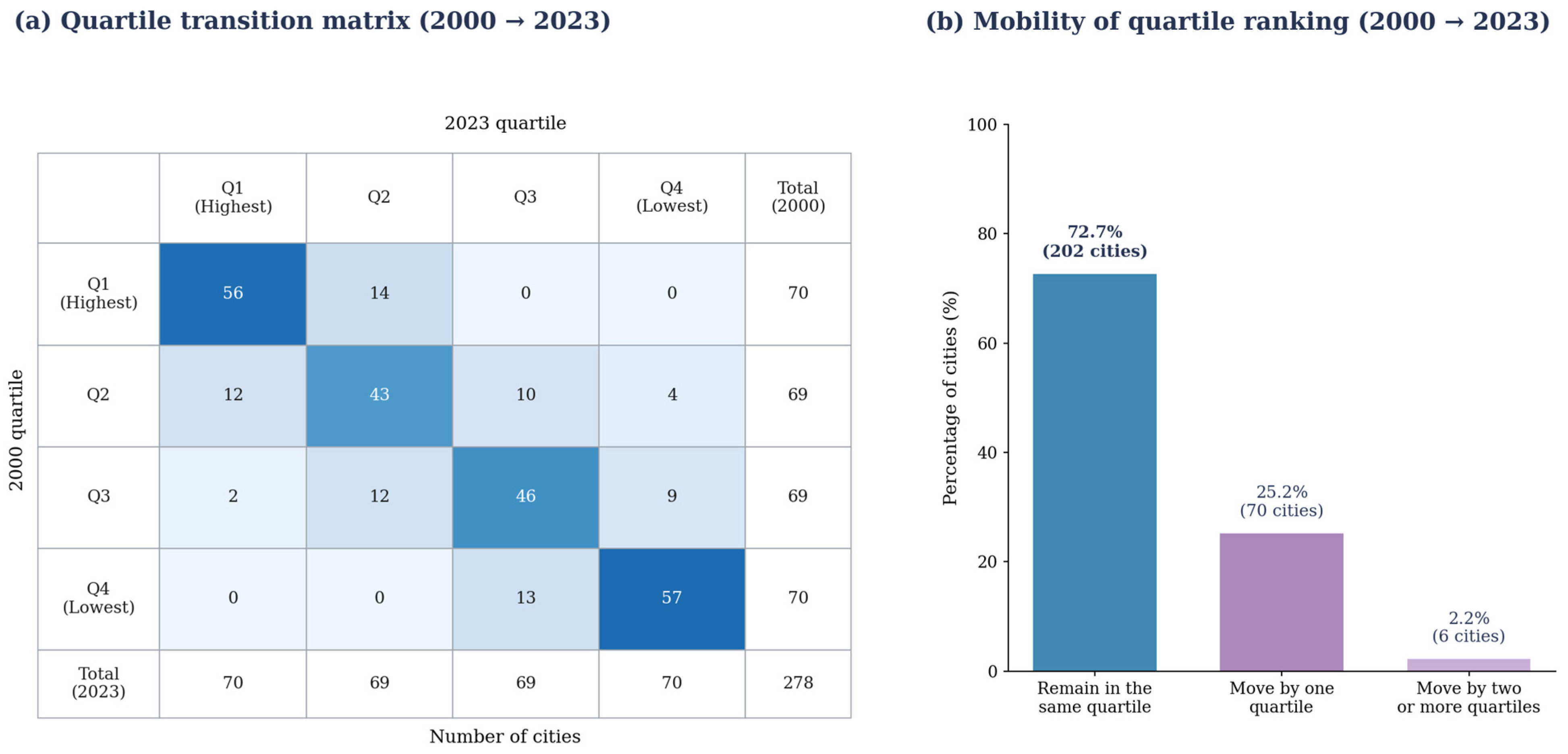
Endpoint road- and market-access rankings are strongly correlated across 2000 and 2023 (Spearman ρ = 0.957 and 0.908, respectively), with 70% top-20 retention for both indicators. Across EMA quartiles, 202 of 278 cities (72.7%) remain in the same endpoint category. Figure 6 reports the complete transition matrix; the quartiles were determined separately by endpoint ranks, not by fixed EMA-score thresholds, and interim moves are not observed.

Figure 6. Quartile transitions and mobility of relative external market accessibility across 278 Chinese cities, 2000–2023.

Figure 6a shows substantial endpoint persistence across the EMA quartile matrix. The diagonal cells contain 56, 43, 46, and 57 cities, totaling 202 with matching endpoint quartiles. Figure 6b groups the remaining endpoint displacements: 70 cities (25.2%) differ by one quartile, and six (2.2%) by two or more. Off-diagonal cells identify the direction of these changes, most of which involve neighboring groups. The matrix adds an endpoint categorical view to the rank correlations in Table 3. It is not an annual transition history and does not measure changes in absolute market access.

Table 3. Persistence and mobility of city-level road and market-access rankings, 2000–2023.

Indicator	Spearman ρ	Top-20 Retention	Median |Δrank|	Mean |Δrank|
RoadTA	0.957	70.0%	9.0	14.9
EMA	0.908	70.0%	13.5	23.3

Rank statistics capture different aspects of hierarchy: overall ordering, persistence among leading cities and movement across endpoint quartiles. A city can gain EMA in absolute index units while slipping in rank as other cities improve faster, and a small difference near a quartile boundary can change its category. The matrix consequently documents selective relative repositioning within a strongly persistent hierarchy; it does not describe an annual Markov transition process.

Rank changes are geographically uneven: 16 of the 20 largest downward EMA movers are in Northeast China (11 Liaoning, four Jilin and one Heilongjiang), whereas the leading upward group includes seven Sichuan, three Henan and three Hunan cities. Initial mean model road time to all other cities is similar for the two groups (19.61 versus 20.64 h), but proximity to leading markets differs markedly: in 2000, the upward group averaged 6.57 h to its nearest top-20-GDP destination, versus only 2.18 h for downward movers. This contrast persists in direction when the hub set is defined using the top 10, 15 or 30 cities. The result suggests that an inherited location near a large economic center does not ensure long-run improvement in relative market rank. It is consistent with the Northeast concentration of downward mobility and the changing weight of its neighboring destinations; explaining firm location, freight and industrial restructuring would require additional evidence.

4.4. Divergent Regional Accessibility Trajectories

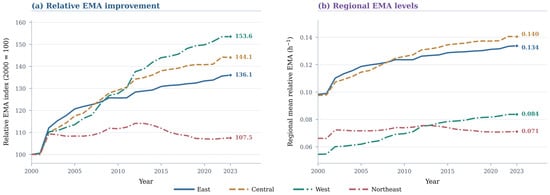
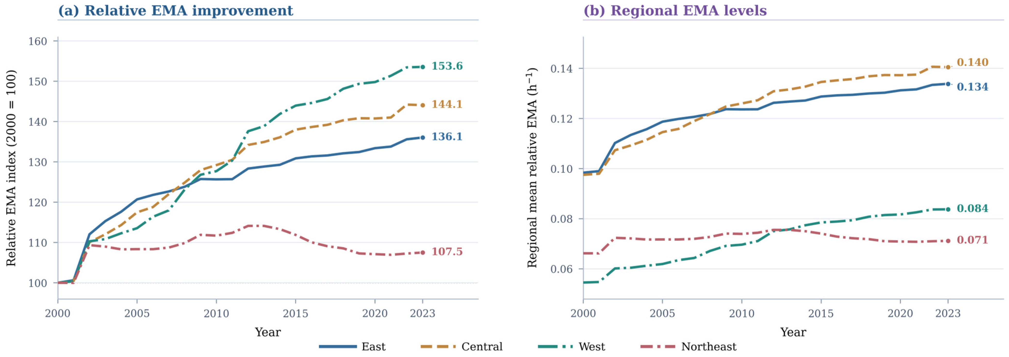
Figure 7 compares proportional EMA changes with their 2023 levels; these need not produce the same regional ordering. The West records the largest 2000–2023 proportional EMA increase (53.6%) from a relatively low base, while the Central region increases by 44.1%. Within the fixed sample, Northeast cities’ share of current-price GDP falls from 9.25% in 2000 to 4.76% in 2023; this is a relative recorded-production shift, not evidence of falling real output or observed intercity trade. The macroregional subsamples contain unequal numbers of cities (84 East, 80 Central, 82 West, 32 Northeast), and the full provincial composition is shown in Table A4. Therefore, regional comparisons depend both on which origins and destinations enter the sample and on where their GDP is located. The city-equal results describe sampled cities; they do not claim to be population-weighted or economy-wide estimates of regional welfare.

Figure 7. Regional trajectories of relative external market accessibility in China, 2000–2023.

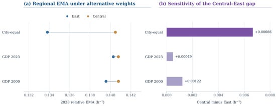
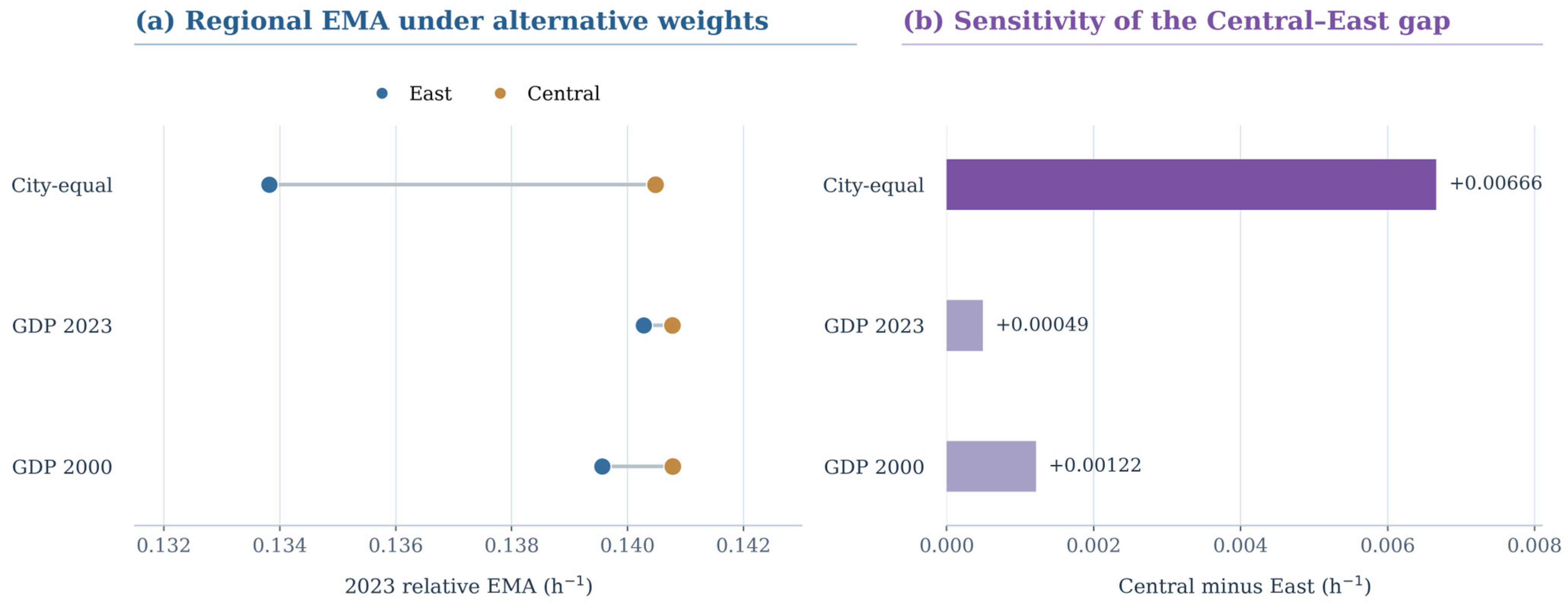
In city-equal regional means, Central China moved from 0.0975 in 2000, just below the East’s 0.0984, to 0.1405 in 2023, above the East’s 0.1338. Figure 8 shows that the 2023 Central–East difference falls from 0.00666 under city-equal averaging to 0.00049 with contemporaneous origin-GDP weights and 0.00122 with fixed-2000 GDP weights. Northeast RoadTA rose by 29.0% while EMA increased by 7.5% under the baseline decay exponent. Northeast EMA peaked around 2010 and stood near 0.071 in 2023; its growth sign varies with the decay parameter (Table A3), although it remains the slowest-improving region in the examined specifications.

Figure 8. Sensitivity of the East–Central comparison in relative external market accessibility to regional aggregation weights in 2023. Note: GDP weights are normalized within each region. Panel (a) uses a narrowed axis; panel (b) begins at zero.

The three regional averages in Figure 8a use identical city-level EMA values but different weights for summarizing origin cities. The city-equal series characterizes the sampled city as the observational unit; the current- and base-year GDP-weighted alternatives give greater influence to larger urban economies. Central China remains narrowly above the East under each rule, while the difference approaches zero under contemporaneous GDP weighting.

Three comparisons must therefore remain separate: proportional EMA improvement versus final index level, city-equal versus GDP-weighted origin averages, and changes in the relative economic composition of destinations. The West’s faster proportional gain does not eliminate its lower starting level; Central China’s small lead over the East is aggregation-sensitive; and the Northeast’s weakening share of the study-area GDP pool is consistent with—but does not alone prove the mechanism behind—its negative origin-specific destination-share term. Section 5.3 interprets these patterns within their sampling and normalization boundaries.

4.5. Network Improvement Versus Market Redistribution

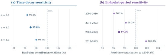
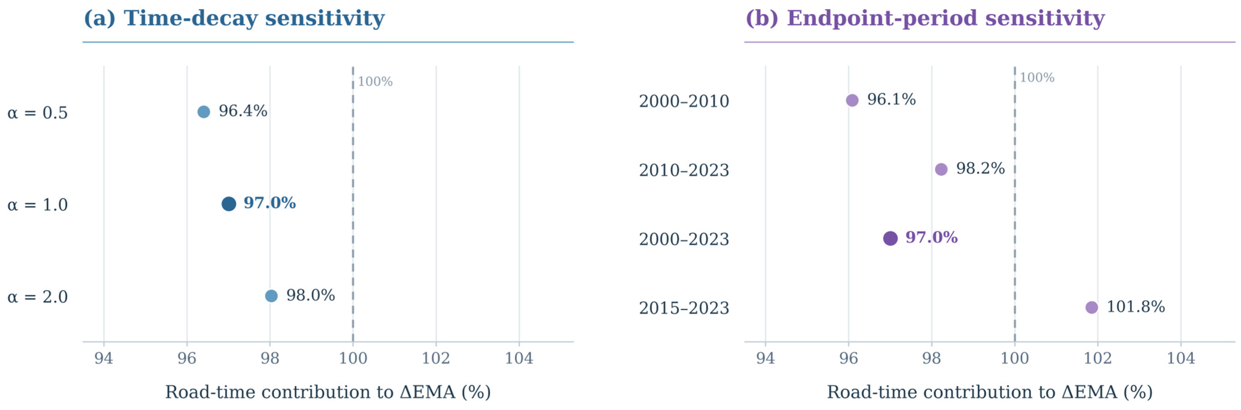
Table 4 reports the two-factor Shapley decomposition of relative EMA over 2000–2023. Rebuilding the four bilateral road-time/GDP-share counterfactuals from all 38,503 OD city pairs yields a national road-time contribution of +0.03130519 (97.0046% of ΔEMA) and a destination-GDP-share contribution of +0.00096666 (2.9954%). Both city EMA endpoints agree with the archived panel to numerical precision. Recalculation over alternative intervals also shows a dominant national road-time term: 96.08% for 2000–2010 and 98.22% for 2010–2023, versus 101.85% for 2015–2023, when the relative GDP-share term turns negative (Figure 9).

Table 4. Regional accessibility changes and two-factor decomposition, 2000–2023.

Region	Cities	EMA 2000	EMA 2023	ΔEMA	Road-Time Term	GDP-Share Term
National	278	0.0815	0.1138	+0.0323	+0.0313	+0.0010
East	84	0.0984	0.1338	+0.0355	+0.0349	+0.0006
Central	80	0.0975	0.1405	+0.0430	+0.0391	+0.0039
West	82	0.0545	0.0837	+0.0292	+0.0266	+0.0026
Northeast	32	0.0662	0.0712	+0.0050	+0.0145	−0.0096

Note: EMA levels and Shapley components are in h⁻¹; baseline time-decay exponent α = 1.

Figure 9. Robustness of the road-time contribution to changes in relative external market accessibility: (a) alternative time-decay exponents; (b) alternative decomposition intervals.

For the Northeast, the road-time component is +0.0145 and the GDP-share component −0.0096. The negative term offsets approximately 65.8% of the positive network contribution. Unlike the national average, the regional total therefore reflects two large components of opposing sign. Section 5.3 discusses the regional implications of this offset.

Across α = 0.5, 1 and 2, the Northeast GDP-share contribution is negative (−0.012676, −0.009555 and −0.004413, respectively), while the road-time term remains positive. The corresponding offset ratios are 46.8%, 65.8% and 112.7%; the region’s net EMA growth is +6.06%, +7.51% and −4.48%. Fixed-2000 and fixed-2023 origin-GDP weights and the alternative common-GDP denominator preserve the negative contribution (Table A3). These results locate a persistent signed component while showing that its strength and the sign of net change depend on measurement assumptions.

An additional price-proxy check uses reported annual city GDP growth rates to chain 2000 economic mass forward on the 275-city complete-rate subset. Under α = 1, the nominal GDP-share contribution is −0.009556 and the growth-chained counterpart is −0.005568; the offset ratio decreases from 65.77% to 37.11%. At α = 0.5 and 2, the GDP-share contribution also remains negative, but net growth at α = 2 switches from negative under nominal GDP (−4.45%) to positive under the growth-chained opportunity proxy (+16.66%). The proxy is informative about price sensitivity, yet the implied city price factors are affected by statistical-vintage and boundary consistency; results are reported as exploratory rather than as an independently validated real-price panel (Table A3).

The national road-time component accounts for 97.0% of the observed baseline EMA increase, yet signed GDP-share components vary by region. A small national net share contribution consequently conceals opposing local reallocations. Table 4 reports component levels, Figure 9 shows the main sensitivity patterns, and Table A5 retains the period-specific accounting terms.

Across the four macroregions, the baseline GDP-share term is positive in the East (+0.0006), Central (+0.0039), and West (+0.0026), but negative in the Northeast (−0.0096); road-time contributions are positive throughout. The Northeast contrast is therefore a distributional finding rather than a mechanically uniform national effect.

Disaggregating the Northeast GDP-share term by destination region identifies other Northeast cities as the main source (−0.010675), followed by the East (−0.001311), while Central and Western destinations offset part of the negative contribution (+0.001041 and +0.001390). The four signed terms sum to −0.009555.

The associated mean origin-specific GDP shares for Northeast destinations fell from 8.99% to 4.62% (−4.37 percentage points). Shares to Eastern destinations also eased (−0.96 points), while Central and Western shares increased (+2.11 and +3.22 points). This geography helps pinpoint which neighboring markets changed in relative weight and motivates investigation of the relevant industries and freight links.

5. Discussion

5.1. Network Reach and Relative Market Opportunities

RoadTA and relative EMA capture different dimensions of access: the first summarizes physical reach, while the second incorporates the relative geography of external GDP. Northeast China’s positive road-time contribution is partly offset by changes in destination shares, which the national mean obscures. The inclusion of home-city GDP also changes the question being answered. Among Northeast origins, self-inclusive coverage of the sample economy within 3 and 6 road-travel hours fell from 1.72% to 1.41% and from 5.76% to 5.04%, respectively, while 12-h coverage rose from 17.50% to 18.43% (Table A1). These threshold shares include home-city GDP and therefore complement, rather than replicate, the origin-excluded inverse-time EMA decomposition.

At the bilateral level, travel time determines the impedance of individual links; at the origin level, GDP shares allocate opportunity weights; and at the regional level, aggregation defines whose access is summarized. Explicitly reporting those choices turns accessibility monitoring into an interpretable diagnostic rather than a single opaque ranking.

Normalization supplies the interpretation boundary for the national 97.0% decomposition share: it allocates movements within the relative EMA measure, not 97.0% of economic growth. The common denominator produces a similar Northeast sign, while nominal market potential captures GDP scale. The growth-chained 275-city comparison adds a substantive caution: price treatment attenuates the negative share term and can reverse the sign of net Northeast EMA at α = 2 (Table A3).

5.2. Inequality, Geographic Clustering and Ranking Stability

The inequality diagnostics establish a substantive, not merely mathematical, distinction: from 2000 to 2023, the national EMA mean increased, the Gini eventually declined, but the mean absolute difference across city pairs rose from 0.031480 to 0.041343 h⁻¹. This implies compression relative to a rising mean, not elimination of the distance between city-level opportunity scores. The geography of mobility is also uneven: 16 of the 20 largest downward EMA movers are Northeast cities (Section 4.3). These facts strengthen the interpretation of durable territorial hierarchy without equating city-level scores with resident-level transport equity.

The spatial evidence is consistent with this asymmetry. Both endpoints display strong positive Moran’s I under the stated k = 5 graph, and high- and low-value clusters remain geographically concentrated. Because the rise in Moran’s I was not subjected to a formal test of between-year differences, we describe it as an observed increase rather than a statistically established structural shift; local classifications use nominal unadjusted tests (Section 4.2).

A planning-oriented cohesion assessment should therefore keep the units of comparison visible: relative dispersion, absolute gaps, neighborhood association and city-rank movements do not measure the same outcome [18,32]. This matters especially when some regional economies become less prominent destinations despite shorter modeled road journeys. Observed freight, employment or household-level service data would be required to decide whether these city-level disparities correspond to unequal outcomes for people or firms.

Reporting these dimensions together changes the follow-up question. Rather than asking whether a lower Gini means that territorial inequality has been solved, analysts can identify cities that remained distant in index levels or fell in rank, examine their accessible destination groups, and test the corresponding realized transport and commercial relationships. This is the most defensible bridge from aggregate maps and ranks to region-specific further investigation.

5.3. Regional Differentiation and the Northeast Connectivity–Market Gap

Regional comparisons depend on both the sample of cities and their weights. West China records the largest proportional EMA gain from a lower baseline, whereas Central China’s narrow city-equal 2023 lead over the East shrinks under GDP weighting. Northeast China’s share of sampled nominal GDP falls from 9.25% to 4.76% over 2000–2023, consistent with a changing relative production landscape. Uneven sample coverage and historical statistical boundaries make the choice of origin and destination universe consequential (Table A4).

Origin-GDP aggregation weights summarize the relative importance of cities, whereas destination GDP shares describe the economic opportunities accessible to each city. The negative Northeast destination-share term persists when origin weights are fixed at 2000 or 2023, which supports the regional interpretation without imposing a single welfare ranking (Table A3).

The Northeast illustrates how improved modeled roads can coexist with a much smaller increase in relative market opportunity. At α = 1, road-time gains (+0.014523) are offset by a negative destination-share contribution (−0.009555), or 65.8% of the positive term. Its negative sign survives the tested nominal-GDP decay, fixed origin-weight and denominator variants, and all 32 Northeast origin cities contribute negatively. However, the growth-chained comparable-price proxy reduces the offset to 37.11% on a common 275-city subset, while changing the net EMA sign at α = 2. The central empirical contribution is thus the persistent direction of the composition effect, accompanied by substantial sensitivity in its magnitude and interpretation.

Destination attribution traces the largest negative contribution to other Northeast cities, whose average external GDP weight drops from 8.99% to 4.62%. This regional reorientation offers an economic-geography interpretation of the rank results: many downward-moving Northeast origins began closer to major markets than rapidly rising cities, yet proximity alone could not preserve their relative position. Possible explanations include uneven structural transformation, changes in industrial demand and changing intercity logistics networks. The indicators identify where these mechanisms should be investigated; future work can examine actual sectoral trade, freight and firm connections.

A planning application can accordingly distinguish network investment from destination-market development: locate weak relative opportunity gains, identify the destination groups involved, compare plausible indicator definitions, then target field evidence toward industries, logistics services and affected populations. The resulting decisions should draw on independent economic and transport appraisal.

5.4. Implications for Sustainable Accessibility Monitoring

The monitoring protocol has three layers: physical network reach, explicitly defined economic or service opportunities, and distributional/geographic persistence, followed where needed by a destination-attribution audit (Table 5). Its information value connects to the planning concerns of SDG 9, particularly reliable and inclusive infrastructure (Target 9.1), and SDG 11, particularly accessible transport and integrated urban planning (Targets 11.2–11.3). We do not measure the UN indicators or any SDG target achievement; instead, the framework helps planners screen where a network improvement might coexist with weak relative opportunity gains and where actual access, users, environmental effects and distributional impacts require evaluation [4,18].

Table 5. Operational monitoring framework for distinguishing road reach, market opportunities and spatial distribution.

Monitoring Layer	Core Indicators	Primary Interpretation	Follow-Up When Signals Diverge
Network reach	Mean intercity road time; RoadTA	Modeled physical connectivity, independent of destination GDP	Inspect OD coverage, network convention and threshold choices
Opportunity-weighted reach	EMA; common-denominator EMA; nominal potential as scope check	Relative destination GDP opportunity at modeled road costs	Examine the destination GDP-share distribution and origin exclusion
Distribution and geography	Gini; Moran’s I; city quartile mobility	Relative inequality, geographic clustering and hierarchical persistence	Evaluate spatial weights, regional boundaries and aggregation rules
Regional counterfactuals	Shapley time and GDP-share components; destination-group allocation	Sources of changes within the defined relative index	Review endpoint/decay sensitivity before investigating observed economic outcomes
Illustrative Northeast case	α = 1: road-time +0.0145; GDP-share −0.0096	Network progress; relative opportunity offset	Examine freight and industrial links before project appraisal

An operational application requires four checks: retain a documented and consistent destination universe; publish the network and opportunity measures separately; report relative and absolute inequality together with cluster and rank persistence; and identify destination groups behind exceptional offsets. Where disparities emerge, regional analysts can then commission information on observed freight journeys, service frequency, generalized costs, trade links and affected users. The framework could be adapted for rail, multimodal transport or another country only after redefining the opportunity set, observed impedance, regional aggregation and beneficiaries; GDP is not a universal proxy for employment, healthcare or environmental sustainability.

For a Northeast planning authority, the contrast between the positive road-time contribution and the negative GDP-share component points first to other Northeast destinations, whose relative GDP shares decreased sharply. The practical next step is to audit intercity freight flows, major buyers and suppliers, transport reliability and sector-specific demand before prioritizing infrastructure or economic development interventions. This turns the decomposition into an evidence-gathering sequence that can complement the sustainable infrastructure and accessibility concerns of SDG 9 and SDG 11.

The same reporting logic can be applied to rail or multimodal systems, and to employment or service opportunities, provided the relevant OD impedance, beneficiaries and opportunity denominator are defined consistently.

5.5. Scope and Limitations

The study evaluates potential access through modeled shortest road times and GDP-weighted destinations. It has a fixed but incomplete 278-city spatial universe, uses current-price GDP in the principal results, and does not observe actual passenger or freight generalized costs, intercity trade or within-city accessibility. These features delineate the population, geography and substantive outcome to which results apply.

Several sensitivities sharpen this boundary. Excluding six known cross-city administrative adjustment cases from both origin and destination sets leaves the Northeast nominal offset near baseline (Table A3), but does not reconstruct every historical city boundary. The province-by-province sample profile is reported in Table A4. The growth-chained price proxy built from reported city growth rates retains the negative Northeast GDP-share component; nevertheless, missing growth histories remove three origins, revision vintages may differ across GDP fields, and resulting implicit price factors are not independently audited deflators. The offset magnitude and net EMA growth change materially under this proxy and across decay functions (Table A3). Interpretation should therefore emphasize the signed within-index regional contrast, together with its economic and statistical measurement conditions.

Subsequent validation could compare modeled OD times with passenger and freight journeys, test links with observed trade and firm transactions, reconstruct historically consistent territories where feasible, and use officially harmonized long-run regional price indices. This would reveal whether the detected pattern predicts actual economic opportunity and sustainability outcomes.

6. Conclusions and Policy Implications

The three research questions lead to three principal conclusions. First, modeled intercity travel time across the fixed 278-city system declined by 28.7% during 2000–2023, and relative EMA increased by 39.6%, but improved network performance did not translate into uniform regional relative-opportunity gains. The West improved fastest proportionally from a lower level, and the Northeast improved the slowest under the baseline measure.

Second, lower relative EMA inequality after 2010 did not mean that the absolute gap or geographical hierarchy disappeared: the absolute mean city-pair difference widened, Moran’s I remained high, and 202 cities occupied the same endpoint quartile. The largest downward movements were geographically concentrated—16 of the 20 were in Northeast China—rather than evenly distributed across the study cities. These are city-level indicator patterns, not evidence of realized household transport equity.

Third, the two-factor Shapley accounting allocates 97.0% of the national relative EMA change to road-time variation under the baseline definition. In the Northeast, the negative destination-share term offsets 65.8% of the positive road-time contribution and is concentrated in other Northeast destinations. Its sign survives multiple nominal-GDP definitions, the joint administrative exclusion, and an exploratory growth-chained GDP comparison; the latter reduces the baseline-alpha offset to 37.11% on a matched 275-city sample. The magnitude of the offset and even the sign of net Northeast EMA movement change across measurement choices. The result is a robust signed regional contrast with clearly identified quantitative limits.

These findings motivate a practical reporting rule: compare physical reach and relative opportunity separately, examine absolute as well as relative and spatial disparities, and trace destination shares before drawing investment priorities. This screening logic is potentially useful beyond China, including multimodal or service-access settings, only after the relevant opportunity universe, travel cost, beneficiaries and administrative coverage have been redefined.

The sustainable-planning contribution is a transparent sequence for locating connectivity–opportunity divergences and tracing their destinations. Such evidence can guide the collection of actual logistics, firm-linkage, resident-access and environmental data needed for regional investment decisions.

Future work should integrate observed travel costs and freight reliability, intercity trade and firm links, resident-level access to employment and services, consistent administrative geographies, and a fully harmonized official regional GDP deflator series.

References

- Harris, C.D. The market as a factor in the localization of industry in the United States. Ann. Assoc. Am. Geogr. 1954, 44, 315–348. [Google Scholar] [CrossRef] [Scilit]
- Hansen, W.G. How accessibility shapes land use. J. Am. Inst. Plan. 1959, 25, 73–76. [Google Scholar] [CrossRef] [Scilit]
- Geurs, K.T.; van Wee, B. Accessibility evaluation of land-use and transport strategies: Review and research directions. J. Transp. Geogr. 2004, 12, 127–140. [Google Scholar] [CrossRef] [Scilit]
- Pot, F.; Rauws, W.; Ramezani, S.; Kajosaari, A.; Humer, A. Principles for place-based accessibility planning. J. Transp. Geogr. 2026, 132, 104588. [Google Scholar] [CrossRef] [Scilit]
- Faber, B. Trade integration, market size, and industrialization: Evidence from China’s National Trunk Highway System. Rev. Econ. Stud. 2014, 81, 1046–1070. [Google Scholar] [CrossRef] [Scilit]
- Baum-Snow, N.; Brandt, L.; Henderson, J.V.; Turner, M.A.; Zhang, Q. Roads, railroads, and decentralization of Chinese cities. Rev. Econ. Stat. 2017, 99, 435–448. [Google Scholar] [CrossRef] [Scilit]
- Banerjee, A.; Duflo, E.; Qian, N. On the road: Access to transportation infrastructure and economic growth in China. J. Dev. Econ. 2020, 145, 102442. [Google Scholar] [CrossRef] [Scilit]
- Wang, J.; Jin, F.; Mo, H.; Wang, F. Spatiotemporal evolution of China’s railway network in the 20th century: An accessibility approach. Transp. Res. Part A Policy Pract. 2009, 43, 765–778. [Google Scholar] [CrossRef] [Scilit]
- Jin, F.; Wang, C.; Li, X.; Wang, J. China’s regional transport dominance: Density, proximity, and accessibility. J. Geogr. Sci. 2010, 20, 295–309. [Google Scholar] [CrossRef] [Scilit]
- Hou, Q.; Li, S.-M. Transport infrastructure development and changing spatial accessibility in the Greater Pearl River Delta, China, 1990–2020. J. Transp. Geogr. 2011, 19, 1350–1360. [Google Scholar] [CrossRef] [Scilit]
- Jiao, J.; Wang, J.; Jin, F.; Dunford, M. Impacts on accessibility of China’s present and future HSR network. J. Transp. Geogr. 2014, 40, 123–132. [Google Scholar] [CrossRef] [Scilit]
- Luo, H.; Zhao, S. Impacts of high-speed rail on the inequality of intercity accessibility: A case study of Liaoning Province, China. J. Transp. Geogr. 2021, 90, 102920. [Google Scholar] [CrossRef] [Scilit]
- Lyu, D.; Zhao, P. How does land transport accessibility reshape population distribution? Long-term dynamics and spatial heterogeneity in China. J. Transp. Geogr. 2026, 136, 104723. [Google Scholar] [CrossRef] [Scilit]
- Wang, L.; Song, A.; Zhang, Z. Geographical constraints and the dual impacts on urban form and accessibility: Lessons from 288 Chinese cities. Sustain. Cities Soc. 2026, 142, 107308. [Google Scholar] [CrossRef] [Scilit]
- Ma, L.; Tang, Y. The distributional impacts of transportation networks in China. J. Int. Econ. 2024, 148, 103873. [Google Scholar] [CrossRef] [Scilit]
- Morris, J.M.; Dumble, P.L.; Wigan, M.R. Accessibility indicators for transport planning. Transp. Res. Part A Gen. 1979, 13, 91–109. [Google Scholar] [CrossRef] [Scilit]
- Kwan, M.-P. Space-time and integral measures of individual accessibility: A comparative analysis using a point-based framework. Geogr. Anal. 1998, 30, 191–216. [Google Scholar] [CrossRef] [Scilit]
- Pereira, R.H.M.; Schwanen, T.; Banister, D. Distributive justice and equity in transportation. Transp. Rev. 2017, 37, 170–191. [Google Scholar] [CrossRef] [Scilit]
- Handy, S.L.; Niemeier, D.A. Measuring accessibility: An exploration of issues and alternatives. Environ. Plan. A 1997, 29, 1175–1194. [Google Scholar] [CrossRef] [Scilit]
- Bruinsma, F.; Rietveld, P. The accessibility of European cities: Theoretical framework and comparison of approaches. Environ. Plan. A 1998, 30, 499–521. [Google Scholar] [CrossRef] [Scilit]
- Levinson, D.M. Accessibility and the journey to work. J. Transp. Geogr. 1998, 6, 11–21. [Google Scholar] [CrossRef] [Scilit]
- Páez, A.; Scott, D.M.; Morency, C. Measuring accessibility: Positive and normative implementations of various accessibility indicators. J. Transp. Geogr. 2012, 25, 141–153. [Google Scholar] [CrossRef] [Scilit]
- Gutiérrez, J. Location, economic potential and daily accessibility: An analysis of the accessibility impact of the high-speed line Madrid–Barcelona–French border. J. Transp. Geogr. 2001, 9, 229–242. [Google Scholar] [CrossRef] [Scilit]
- Redding, S.; Venables, A.J. Economic geography and international inequality. J. Int. Econ. 2004, 62, 53–82. [Google Scholar] [CrossRef] [Scilit]
- Donaldson, D.; Hornbeck, R. Railroads and American economic growth: A ‘market access’ approach. Q. J. Econ. 2016, 131, 799–858. [Google Scholar] [CrossRef] [Scilit]
- Vickerman, R.; Spiekermann, K.; Wegener, M. Accessibility and economic development in Europe. Reg. Stud. 1999, 33, 1–15. [Google Scholar] [CrossRef] [Scilit]
- Zheng, S.; Kahn, M.E. China’s bullet trains facilitate market integration and mitigate the cost of megacity growth. Proc. Natl. Acad. Sci. USA 2013, 110, E1248–E1253. [Google Scholar] [CrossRef] [Scilit] [PubMed]
- Lin, Y. Travel costs and urban specialization patterns: Evidence from China’s high speed railway system. J. Urban Econ. 2017, 98, 98–123. [Google Scholar] [CrossRef] [Scilit]
- Yu, N.; de Roo, G.; de Jong, M.; Storm, S. Does the expansion of a motorway network lead to economic agglomeration? Evidence from China. Transp. Policy 2016, 45, 218–227. [Google Scholar] [CrossRef] [Scilit]
- Qin, Y. ‘No county left behind?’ The distributional impact of high-speed rail upgrades in China. J. Econ. Geogr. 2017, 17, 489–520. [Google Scholar] [CrossRef] [Scilit]
- Gutiérrez, J.; Urbano, P. Accessibility in the European Union: The impact of the trans-European road network. J. Transp. Geogr. 1996, 4, 15–25. [Google Scholar] [CrossRef] [Scilit]
- López, E.; Gutiérrez, J.; Gómez, G. Measuring regional cohesion effects of large-scale transport infrastructure investments: An accessibility approach. Eur. Plan. Stud. 2008, 16, 277–301. [Google Scholar] [CrossRef] [Scilit]
- Gutiérrez, J.; Condeço-Melhorado, A.; Martín, J.C. Using accessibility indicators and GIS to assess spatial spillovers of transport infrastructure investment. J. Transp. Geogr. 2010, 18, 141–152. [Google Scholar] [CrossRef] [Scilit]
- Cao, J.; Liu, X.C.; Wang, Y.; Li, Q. Accessibility impacts of China’s high-speed rail network. J. Transp. Geogr. 2013, 28, 12–21. [Google Scholar] [CrossRef] [Scilit]
- Shaw, S.-L.; Fang, Z.; Lu, S.; Tao, R. Impacts of high speed rail on railroad network accessibility in China. J. Transp. Geogr. 2014, 40, 112–122. [Google Scholar] [CrossRef] [Scilit]
- Cabello, M.; Hyland, M.; Marantz, N. From state of the practice to state of the art: Improving equity analysis in regional transportation plans. Transportation 2025, 52, 791–826. [Google Scholar] [CrossRef] [Scilit]
- Jiao, J.; Wang, J.; Jin, F.; Du, C. Understanding relationship between accessibility and economic growth: A case study from China (1990–2010). Chin. Geogr. Sci. 2016, 26, 803–816. [Google Scholar] [CrossRef] [Scilit]
- Condeço-Melhorado, A.; Zofío, J.L.; Christidis, P. Drivers of changes in Spanish accessibility for the 1960–2010 period. Eur. Transp. Res. Rev. 2017, 9, 19. [Google Scholar] [CrossRef] [Scilit]
- Moran, P.A.P. Notes on continuous stochastic phenomena. Biometrika 1950, 37, 17–23. [Google Scholar] [CrossRef] [Scilit]
- Anselin, L. Local indicators of spatial association—LISA. Geogr. Anal. 1995, 27, 93–115. [Google Scholar] [CrossRef] [Scilit]
- Shorrocks, A.F. Decomposition procedures for distributional analysis: A unified framework based on the Shapley value. J. Econ. Inequal. 2013, 11, 99–126. [Google Scholar] [CrossRef] [Scilit]
Disclaimer/Publisher’s Note: The statements, opinions and data contained in all publications are solely those of the individual author(s) and contributor(s) and not of MDPI and/or the editor(s). MDPI and/or the editor(s) disclaim responsibility for any injury to people or property resulting from any ideas, methods, instructions or products referred to in the content. |
© 2026 by the authors. Licensee MDPI, Basel, Switzerland. This article is an open access article distributed under the terms and conditions of the Creative Commons Attribution (CC BY) license.