Thermal Demand-Side Management to Reduce Peak Flows and Support Supply Temperature Reduction in District Heating Networks: A Case Study in Italy

Abstract

Lowering supply temperatures in existing district heating networks facilitates the integration of renewable energy sources and waste heat, but the higher mass flow rates required to maintain heat delivery can introduce hydraulic constraints. This study investigates how thermal demand-side management can create hydraulic margin for supply temperature reduction. A mixed-integer linear programming model optimizes substation start-up shifts within ±15 min, while hydraulic simulations and energy balances assess the resulting operating conditions. The methodology is applied to a district heating network in northern Italy serving 146 substations. An optimized schedule for a single cold reference day reduces the network peak mass flow rate by approximately 23% and reduces daily peaks on all additional days assessed without further optimization. The resulting hydraulic margin accommodates higher mass flow rates, indicating an estimated potential to reduce supply temperatures from 120 °C to approximately 105–108 °C while preserving daily thermal-energy delivery. Hydraulic simulations at daily network peaks show that the baseline minimum substation differential pressure is preserved. These results demonstrate the potential of thermal demand-side management in enabling lower-temperature operation and enhancing the sustainability of existing district heating networks.

1. Introduction

Decarbonizing the heating sector is essential to the energy transition, as heat accounts for the largest share of global final energy consumption and is still heavily reliant on fossil fuels [1]. In Europe, residential heating accounts for a substantial share of energy consumption [2], making the decarbonization of the building sector critical to achieving climate targets [3]. This requires integrating renewable energy sources (RES) and waste heat (WH) into the heat supply, and District Heating (DH) provides an ideal platform for this integration [4,5]. District energy networks are therefore expected to expand, with their contribution projected to reach 20% of global space heating demand by 2030 [6].

Achieving these goals requires not only developing new networks but, above all, upgrading existing DH systems originally designed to rely on fossil fuels and cogeneration. The European Union has established progressively stricter criteria for qualifying as an “efficient district heating and cooling system” under Article 26 of the Energy Efficiency Directive (EU) 2023/1791 [7]: until 2035, a share of at least 80% high-efficiency cogenerated heat is sufficient to meet these criteria; from 2035, compliance requires at least 80% from high-efficiency cogeneration, RES and WH combined, including at least 35% from RES and WH, or at least 50% from RES and WH alone. Subsequent requirements become progressively stricter, reaching 100% RES and WH by 2050.

Research efforts are increasingly focused on developing decarbonization roadmaps to meet these targets [8,9] by maximizing the use of local RES and WH [10,11], integrating heat pumps (HPs) [12,13], and enabling distributed generation [14,15] and the participation of thermal prosumers [16,17]. Potential heat sources include industrial waste heat [18], heat recovered from data centres [19,20] and wastewater [21,22], geothermal energy [23,24], and solar thermal energy [25,26]. Their integration depends not only on local availability and proximity to the network, but also on the compatibility between their temperature levels and those required by the DH system. Lowering network operating temperatures can facilitate this integration while improving the efficiency of several heat production technologies [27,28]. However, these benefits require assessing whether existing DH networks and connected heating systems can operate at lower temperatures while maintaining adequate heat delivery. This assessment includes verifying whether building heating devices can meet the same heat demand at lower temperatures [29], whether substation heat exchangers are adequately sized for these operating conditions [30], and whether the network can accommodate the associated increase in mass flow rates [31].

While previous studies have shown that many existing building heating systems and thermal substations can operate at lower temperatures without significant modifications [32], excessive increases in mass flow rates can limit supply temperature reduction at the network level, particularly in areas already operating close to their hydraulic capacity. Thermal demand-side management (TDSM) strategies can help address this limitation by reshaping heat demand to reduce peak mass flow rates across the network. These strategies have previously been applied to reduce peaks in the heating demand [33,34], decrease energy consumption [35], facilitate DH network expansion into new areas [36,37], reduce pumping costs and enhance overall production efficiency [38,39].

Although these studies demonstrate several operational benefits of TDSM, they do not explicitly assess its use as a means of reducing supply temperature. This study addresses this gap by investigating how the hydraulic margin gained through load shifting can be used to achieve greater reductions in supply temperature. Specifically, this work:

• Develops a TDSM method based on mixed-integer linear programming (MILP) to optimize load shifting and reduce network mass flow peaks.
• Evaluates its effectiveness in reducing peak flows and alleviating hydraulic constraints under current operating conditions.
• Assesses the extent to which these improvements enable supply temperature reduction.

To assess this potential, the proposed methodology is applied to a DH network in Italy, where building heating systems are typically switched off overnight and restarted in the morning, producing pronounced heat demand and mass flow peaks. These operating conditions make the network particularly suited to assessing how TDSM can reduce peak flows and create hydraulic margin for supply temperature reduction.

2. Methodology

Assessing the combined effects of TDSM and supply temperature reduction requires an integrated methodology that captures the resulting changes in DH system operation. The methodology comprises three interconnected components:

• Section 2.1 introduces the DH network model.
• Section 2.2 describes the TDSM optimization framework used to determine the optimal load-shifting strategy.
• Section 2.3 explains how the hydraulic margin obtained from TDSM is used to assess the potential for supply temperature reduction.

2.1. DH Network Model

A detailed hydraulic model of the DH network is used to simulate water circulation in both the supply and return lines. The DH model domain includes only the distribution network, while production plants and substations lie outside its control volume and are represented through boundary conditions. The model solves the mass and momentum conservation equations to determine pressure, mass flow rate, and velocity distributions throughout the network. Hydraulic transients evolve on much shorter timescales than thermal disturbances, allowing a quasi-steady formulation in which the hydraulic equations are solved at successive time steps with updated boundary conditions.

The model is one-dimensional, and the network topology is represented using graph theory, with pipes represented as branches and junctions as nodes. Their connectivity is described by the incidence matrix A, which has NN rows and NB columns, where NN and NB denote the numbers of nodes and branches, respectively. Each element Aij equals 1 if node i is the inlet of branch j, −1 if it is the outlet, and 0 otherwise. The one-dimensional conservation equations are integrated over each pipe using the finite volume method and assembled through this graph representation, yielding the matrix formulation presented in Equation (1).

$$\begin{gathered} \mathit{A}\mathit{G}+{\mathit{G}}_{\mathit{e}\mathit{x}\mathit{t}}=\mathbf{0} \\ {\mathit{A}}^{\mathit{T}}\mathit{P}=\mathit{R}\left(\mathit{G}\right)\mathit{G} \end{gathered}$$

(1)

The unknowns are the vector G, of dimension NB × 1, containing the mass flow rates in all branches, and the vector P, of dimension NN × 1, containing the pressures at all nodes. The matrix R(G) represents the hydraulic resistance of the network pipes. Its dependence on mass flow rate makes the momentum equations nonlinear. Boundary conditions are specified through the vector G_ext, of dimension NN × 1, containing the mass flow rates injected into or extracted from the network nodes, together with a prescribed reference pressure. Production plants inject water into the supply network and withdraw it from the return network, while substations withdraw water from the supply network and inject it into the return network. The resulting system of equations is solved at each time step for both the supply and return networks. For tree-shaped networks, the solution is sequential, with mass flow rates determined from the mass conservation equations before calculating pressures, while looped networks require an iterative approach, such as the SIMPLE algorithm [40] adapted to DH networks by Guelpa et al. [41].

The hydraulic solution provides pressure and mass flow rate distributions throughout the network, from which velocities, pressure drops per unit length, and differential pressures available at substations are calculated. These quantities are used to assess whether the proposed operating strategies remain within hydraulic limits.

The model was previously validated against operational measurements from a large-scale district heating network at a temporal resolution of 10 min [42], while a finer resolution of 5 min is adopted here to better resolve demand variations and peak-flow conditions. In this work, it is first used to simulate current operation at the existing supply temperature, establishing the baseline hydraulic conditions adopted as reference limits. Operation with TDSM is then simulated at the same temperature, using the load-shifting settings obtained from the optimization framework presented in Section 2.2, to quantify the resulting hydraulic margin. Finally, following the procedure described in Section 2.3, the supply temperature is progressively reduced with TDSM applied to determine the maximum reduction achievable while maintaining hydraulic conditions within the baseline limits. This approach provides a conservative estimate of the achievable temperature reduction, as additional hydraulic capacity beyond these reference limits may be available to support further reductions.

2.2. TDSM Through Load Shifting

Active consumer participation through demand-side management can improve energy system operation by aligning demand with available production and network capacity. Widely used in electricity systems, this approach is also increasingly applied to thermal demand in DH through strategies such as changes in heating schedules or control methods. Among these strategies, this study adopts load shifting, which consists of advancing or delaying building heating start-up times after the overnight shutdown. These schedule changes are represented by shifting substation mass flow rate profiles in time while preserving their shape. Although building thermal dynamics may alter these profiles, peak mass flow is primarily constrained by substation operating limits, supporting this simplification for the purposes of the present analysis. The analysis focuses on a network-level perspective, where coincident demand peaks increase aggregate mass flow and pressure losses, potentially creating hydraulic bottlenecks and reducing the differential pressure available at consumer substations. The model therefore assesses how changes in peak timing can alleviate these conditions without explicitly modelling building thermal dynamics. Shifts are applied with a discrete granularity of 5 min (e.g., 5, 10, or 15 min), up to a maximum advance or delay of 15 min. This limit is intended to minimize disturbances to normal heating schedules. Although the present application focuses on load shifting, the overall methodology can be extended to evaluate the effects of other TDSM strategies on network hydraulics and their potential to enable supply temperature reduction.

An optimization model is formulated to select the time shift for each substation that minimizes the daily peak mass flow rate at the plant. The problem is formulated as a MILP by representing the admissible shifts through predefined matrices and introducing binary selection variables and a continuous auxiliary variable for the peak mass flow rate.

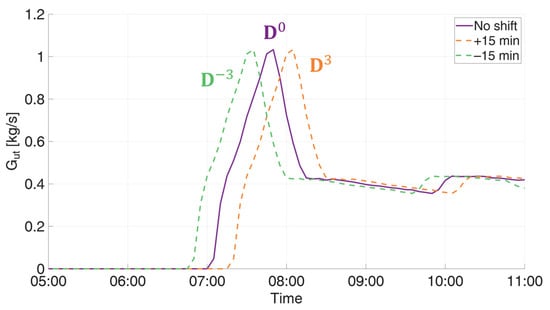
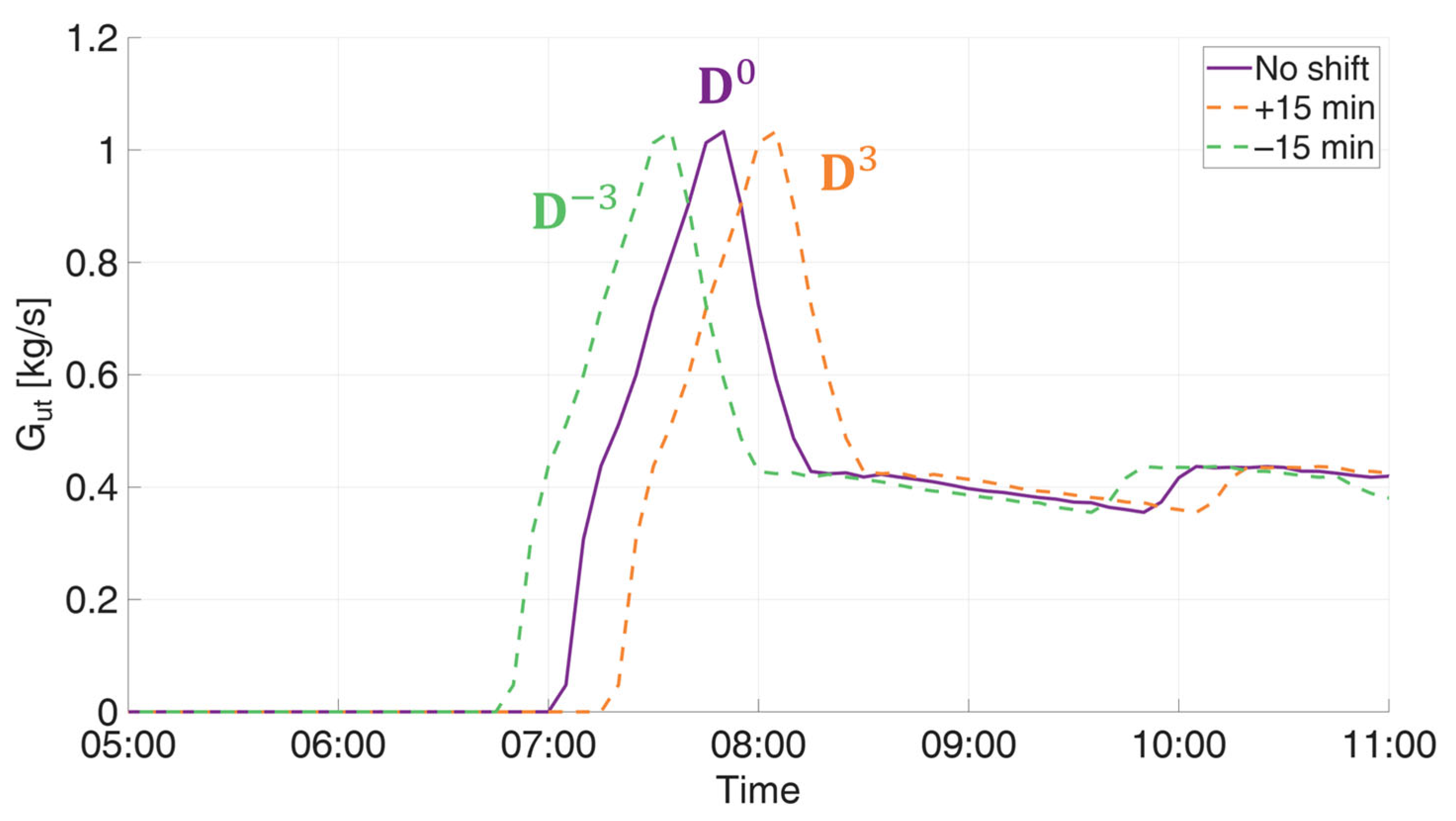
For each substation, candidate mass flow rate profiles are generated by applying predefined shift matrices D^s to the original time-discretized profile G_ext,k where s indexes the admissible options, including advances, delays, and no shift. For example, D⁻¹ applies a 5-min advance, D⁻² a 10-min advance, and D⁻³ a 15-min advance, and matrices D¹, D², D³ apply the corresponding delays. D⁰ is the identity matrix and leaves the profile unchanged. Each candidate profile can therefore be expressed as D^sG_ext,k. An example is provided in Figure 1.

Figure 1. Example of the load shifting strategy.

A binary variable x_k,s is then associated with each candidate profile and equals 1 if option s is selected for substation k and 0 otherwise. The constraint ${\sum }_s{x}_{k,s} = 1$ ensures that exactly one candidate profile is selected for each substation. The resulting profile is therefore given by ${\mathbf{G}}_{\mathit{ext},k}^{\mathit{TDSM}}= {\sum }_s{x}_{k,s} {\mathbf{D}}^s{\mathbf{G}}_{\mathit{ext},k}$, and the plant mass flow rate is obtained by summing these profiles across all substations at each time step. The selected shifts are collected in the vector d, with $d_k={\sum }_{s}s x_{k,s}$. Each component represents the shift in 5-min intervals, with negative values indicating advances and positive values indicating delays.

Finally, to minimize the daily peak, a continuous auxiliary variable G_max, representing the daily peak mass flow rate at the plant, is introduced and constrained to be greater than or equal to the plant mass flow rate at every time step. Minimizing G_max therefore selects the combination of shifts yielding the lowest daily peak.

Since the shift matrices and original mass flow rate profiles are fixed input data, the constraints are linear in the selection variables. Together with the linear objective function and binary selection variables, this yields the MILP formulation presented in Equation (2). The objective is to minimize G_max,. The first constraint requires G_max, to be no smaller than the sum of the substation mass flow rates at every time step; minimizing it therefore identifies the maximum of the aggregate profile. The second constraint constructs each substation’s operating profile by selecting among the admissible time-shifted profiles. The third constraint ensures that exactly one shift, including the option of no shift, is assigned to each substation. Finally, the binary constraint restricts each selection variable to either 0 or 1, preventing combinations of multiple candidate profiles for the same substation.

$$\begin{array}{c}\underset{x,G_{\max }}{\min }\hspace{1em}\hspace{1em}{G}_{\max }\\ \hspace{1em}\hspace{1em} \hspace{1em}\hspace{1em}\hspace{1em}\hspace{1em}\hspace{1em}\hspace{1em}\hspace{1em}\mathrm{s}.\mathrm{t}.\hspace{1em}{G}_{\max }\ge {\displaystyle \sum _k}{G}_{\mathrm{ext},k}^{\mathrm{TDSM}}\left(t\right),\hspace{1em}\forall t\\ \hspace{1em}\hspace{1em}\hspace{1em}\hspace{1em}\hspace{1em}\hspace{1em} \hspace{1em}\hspace{1em}\hspace{1em}\hspace{1em}\hspace{1em}\hspace{1em}\hspace{1em}{\mathbf{G}}_{\mathrm{ext},k}^{\mathrm{TDSM}}={\displaystyle \sum _s}{x}_{k,s}{\mathbf{D}}^s{\mathbf{G}}_{\mathrm{ext},k},\hspace{1em}\forall k\\ \hspace{1em} \hspace{1em}\hspace{1em}\hspace{1em}\hspace{1em}\hspace{1em}\hspace{1em}\hspace{1em}{\displaystyle \sum _s}{x}_{k,s}=1,\hspace{1em}\forall k\\ \hspace{1em}\hspace{1em} \hspace{1em}\hspace{1em}\hspace{1em}\hspace{1em}\hspace{1em}\hspace{1em}\hspace{1em}{x}_{k,s}\in \left\{0,1\right\},\hspace{1em}\forall k,s\end{array}$$

(2)

The model is implemented in Julia [43] and solved using Gurobi [44].

The optimized substation mass flow rate profiles are then used as boundary conditions in the DH network model described in Section 2.1 to assess their effects on operating conditions and quantify the hydraulic margin available for supply temperature reduction.

2.3. Assessment of Potential Supply Temperature Reduction

The load-shifting strategy described in Section 2.2 reduces the aggregate peak at a network level, thus creating a margin that can be used to accommodate higher circulating mass flow rates. This section investigates how that margin can support supply temperature reduction. At unchanged return temperature, lowering the supply temperature reduces the supply-return temperature difference, requiring higher flow rates to maintain the same thermal power delivery. The assessment therefore combines an energy balance with verification of network hydraulic conditions and individual substation flow limits.

In this analysis, the return temperature is assumed to remain unchanged between the current and reduced-supply-temperature scenarios. This assumption is supported by the detailed substation analyses presented in [32,45]. These studies showed that, at a given outdoor temperature and with unchanged secondary-side conditions, the primary return temperature is more strongly influenced by the building-side return temperature than by the primary supply temperature. Consequently, reducing the supply temperature produces only limited changes in the return temperature under the same thermal load conditions.

The potential increase in mass flow rate is quantified by the scaling factor β, defined in Equation (3) as the ratio between the peak network mass flow rate under current operation and that obtained with TDSM on the reference day. Multiplying the TDSM profiles by β restores the aggregate reference-day peak to a flow rate already sustained by the network under current operation.

$$\beta ={\displaystyle \frac{\max G_{\mathit{plant},\mathit{current}}\left(t\right)}{\max G_{\mathit{plant},\mathit{TDSM}}\left(t\right)}}$$

(3)

Assuming unchanged return temperature and constant specific heat capacity, the thermal power balance in Equation (4) determines the corresponding reduced supply temperature. This provides an estimate without explicitly modelling the detailed substation response. A detailed assessment of substation thermal performance and the associated changes in return temperature is reserved for future work.

G_TDSM c_p (T_s,current − T_r) = β G_TDSM c_p (T_s,new − T_r)

(4)

A larger scaling factor allows a greater supply temperature reduction. The increased flow profiles are then imposed as boundary conditions in the hydraulic model described in Section 2.1, maintaining the same differential pressure at the plant. The model verifies local operating conditions throughout the day, accounting for the modified temporal and spatial distribution of flows. This verification is necessary because restoring the aggregate peak to its original value does not necessarily reproduce the original pressure distribution.

The increased mass flow rate profiles are also checked against individual substation limits. For each substation, the maximum flow recorded during the available heating season is adopted as a conservative upper operating limit, since its actual capacity may exceed the highest observed value. If the flow required for reduced-temperature operation exceeds this substation limit, the profile is capped. The resulting reduction in thermal power is compensated by extending heating operation through an earlier start-up, while retaining the scheduled shutdown time. The extension is determined by requiring the integrated thermal power over the day to equal the energy delivered under current operation. Although these adjustments modify the profiles obtained from the initial optimization, they are applied subsequently in this work, without re-optimizing the schedule, retaining the MILP formulation based on predefined profile shifts.

3. Case Study

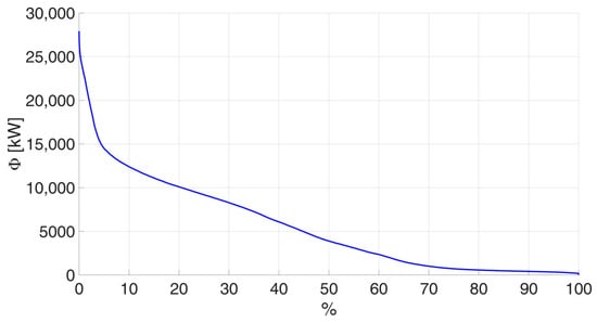
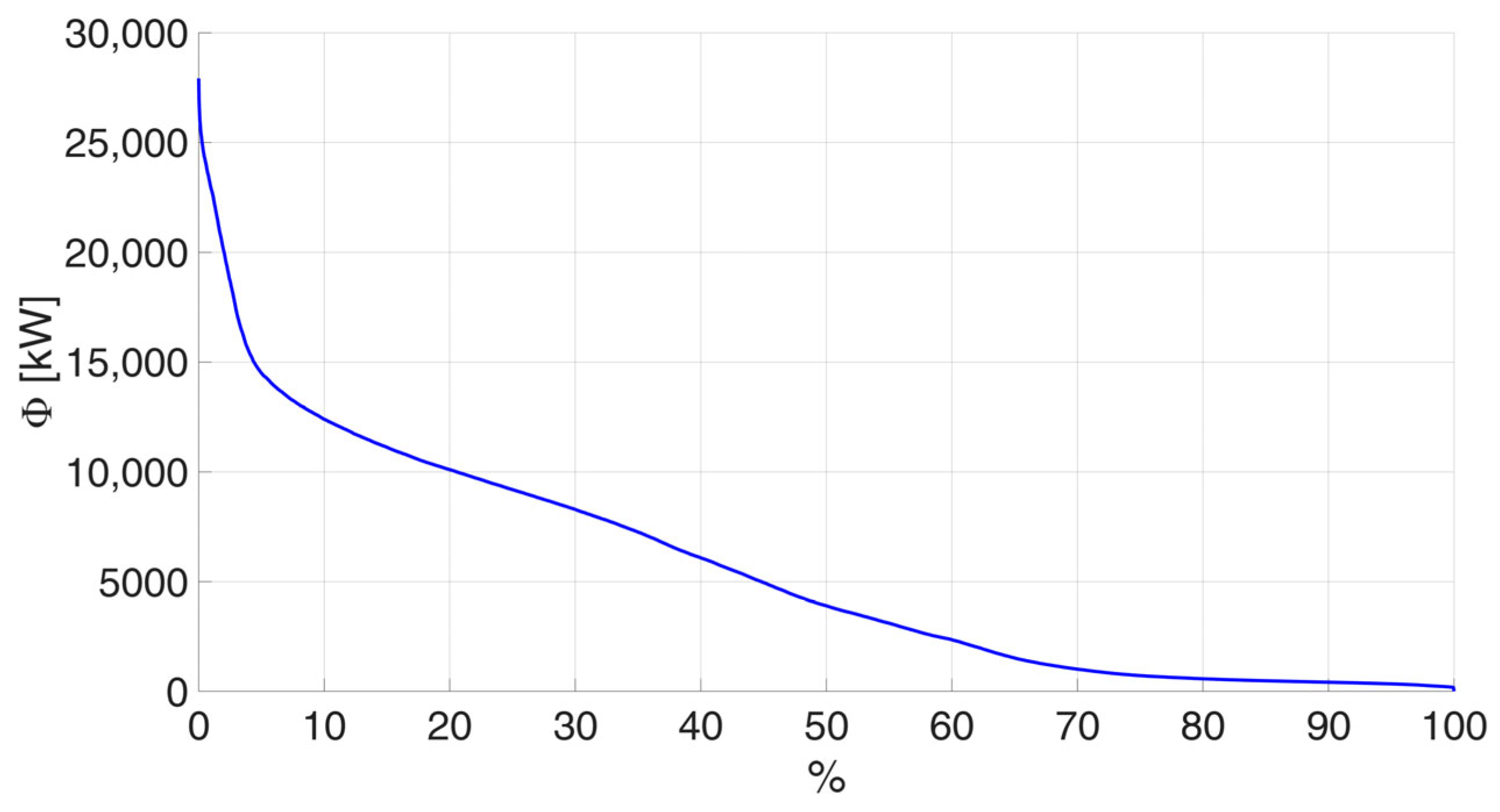
This study analyses a DH network located in northern Italy, comprising over 9 km of pipes (supply and return). The network supplies space heating to 146 substations during the heating season, from 15 October to 15 April. It operates at a supply temperature of 120 °C and a return temperature of approximately 65 °C. Operational data are available for one heating season, during which total heat demand was approximately 30 GWh, with a peak of 27.9 MW. Figure 2 presents the heat load duration curve for this period.

Figure 2. Heat load duration curve for the analysed heating season, expressed as a percentage of operating time.

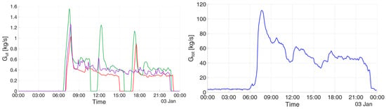
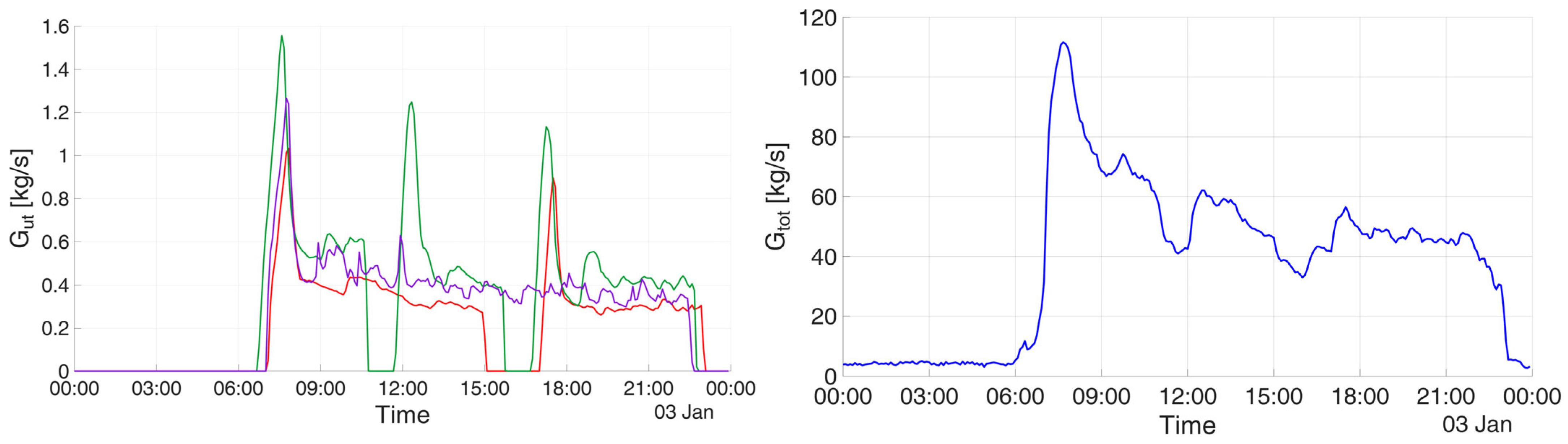
The network exhibits pronounced morning peaks associated with the restart of building heating systems after the overnight shutdown. Figure 3 shows the daily mass flow rate profiles of three representative substations (left) and the aggregate profile of all 146 substations (right). The coincidence of individual peaks produces a marked network peak, making TDSM particularly relevant for reducing peak flows and smoothing the aggregate mass flow rate profile.

Figure 3. Daily mass flow rate profiles for three representative substations, distinguished by color (left) and the aggregate of all 146 substations at network level (right), illustrating the morning peaks associated with heating system start-up.

Although TDSM is applied throughout the heating season, the optimal load-shifting schedule is determined only once by applying the MILP model described in Section 2.2 to a selected operating day. This day has a peak heat demand of approximately 25.7 MW, a value exceeded during less than 0.15% of the seasonal operating time and by the daily peak on only 10% of operating days. It therefore provides a demanding reference condition for assessing the supply temperature reduction enabled by TDSM, which is subsequently evaluated across the entire heating season.

4. Results and Discussion

This section presents and discusses the results of the analysis, which is divided into two parts:

• Section 4.1 analyses the results of TDSM applied to the end users with the aim of reducing the peak flow at the supply node of the network.
• Section 4.2 examines how peak reduction enables lower supply temperatures while accommodating the associated increase in circulating mass flow rates. Substation constraints are also assessed, and heating schedules are adjusted where necessary to ensure that the same amount of thermal energy is delivered to each user.

4.1. Peak Mass Flow Reduction Through TDSM

The MILP model is applied to a cold reference day (3 January) to determine the substation load-shifting schedule that minimizes the peak network mass flow rate. The resulting schedule is then applied unchanged to all other operating days in the heating season.

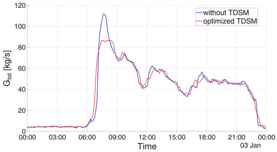
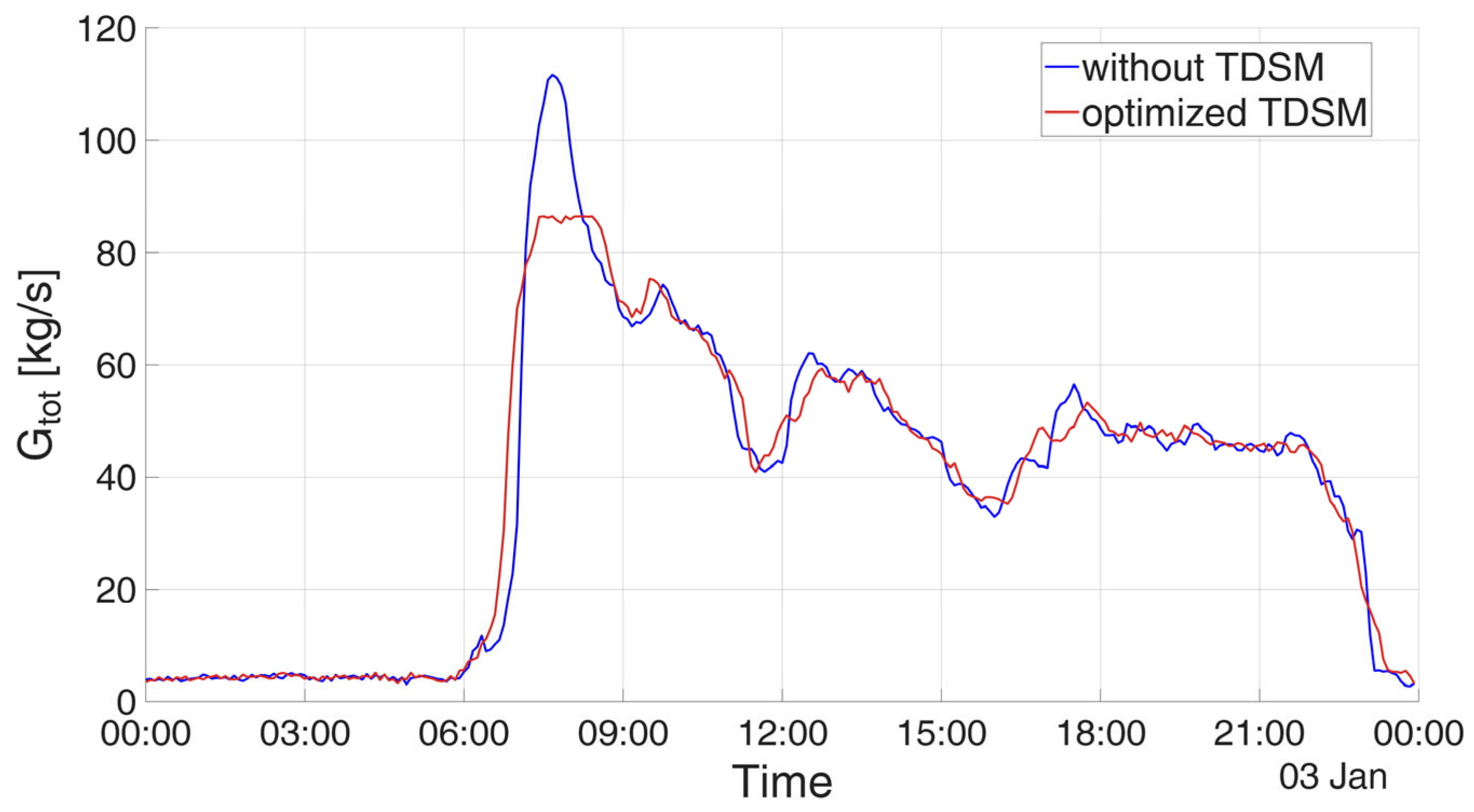
Figure 4 compares the aggregate mass flow rate profiles for the reference day under current operation (blue) and with TDSM (red). The network peak decreases from 111.7 to 86.4 kg/s, corresponding to a reduction of 22.6%.

Figure 4. Aggregate mass flow rate profiles under current operation and with TDSM on the reference day, 3 January.

Table 1 reports the distribution of substation start-up shifts, including advances and delays of 5, 10, and 15 min, obtained from MILP optimization for the reference day. The ±15 min range was selected to limit changes to normal heating schedules and their potential impact on occupant thermal comfort. Most substations are assigned the maximum permitted shift of 15 min, indicating that the optimization makes extensive use of the available scheduling flexibility to reduce the network peak. The predicted reduction therefore depends on the assumed flexibility window: a narrower range could limit the achievable reduction, whereas a wider range could provide additional benefits but would require further evaluation of operational feasibility and thermal comfort.

Table 1. Optimized substation start-up shifts for the reference day. Negative values indicate advances and positive values indicate delays.

Shift [min]	0	−5	−10	−15	+5	+10	+15
Substations [-]	8	4	8	67	9	3	47

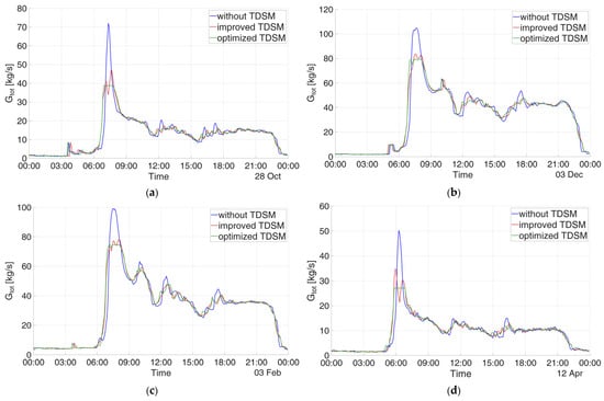
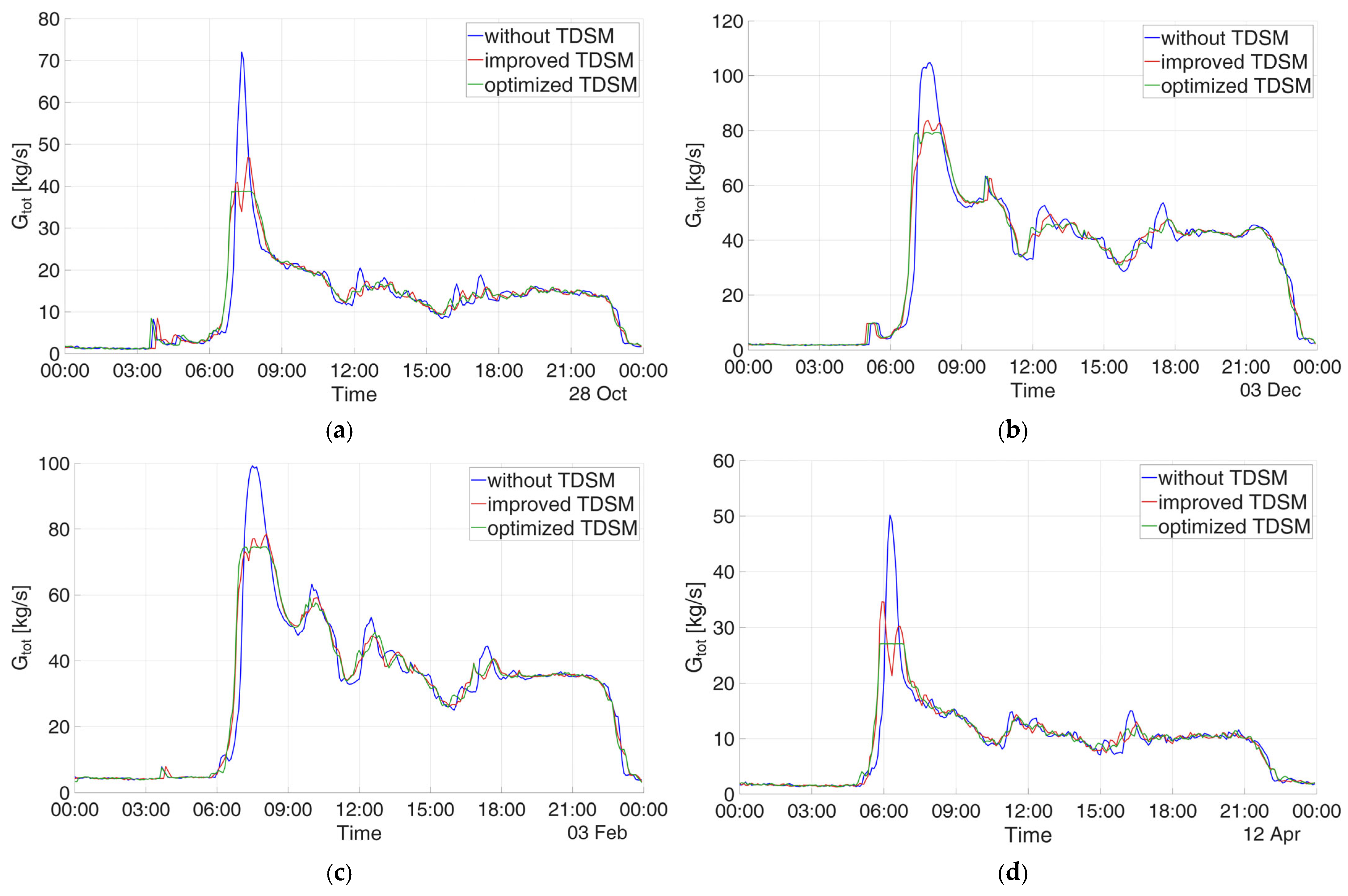
The effectiveness of the reference-day schedule is assessed across days with different heat demands. Since transferring a schedule does not guarantee peak reduction on every day, this is verified a posteriori. To assess the benefit of day-specific schedule optimization, Figure 5 compares two TDSM schedules across four representative days: the improved TDSM schedule (red), obtained by applying the schedule derived from the reference day to the new day, and the optimized TDSM schedule (green), obtained by optimizing the schedule specifically for the day under analysis.

Figure 5. Comparison of current operation, the reference-day TDSM schedule, and four day-specific optimized schedules for 28 October (a), 3 December (b), 3 February (c) and 12 April (d).

On October 28 and April 12 (the days with lower flow rates), the day-specific optimization achieves a peak reduction of 46%, whereas applying the reference-day schedule yields reductions of 35% and 31%, respectively. Similarly, for both December 3 and February 3 (the days with higher flow rates), the day-specific optimization leads to a 24% reduction, compared to the 20% decrease achieved by the reference schedule. These findings demonstrate that although transferring the reference schedule does not yield the optimal result for every day, it captures most of the achievable peak reduction without requiring further day-by-day optimization.

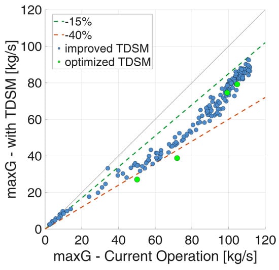
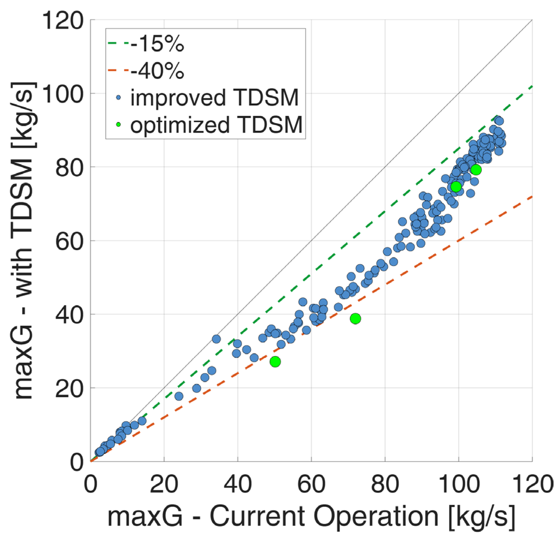
Moreover, to assess the effectiveness of the improved TDSM schedule on the entire period under analysis, Figure 6 compares daily peak mass flow rates under current operation and with improved TDSM. All points lie below the line of equality, confirming a reduction on every day assessed. Reductions are generally around 15% on days with higher peaks and approach 40% on some lower-demand days. Across all days assessed, the highest peak decreases from approximately 110 kg/s under current operation to approximately 90 kg/s with TDSM. The green markers show the results of optimized TDSM for the four selected days discussed above, obtained by optimizing the schedule separately for each day. These points lie within or close to the cloud associated with improved TDSM, although daily optimization provides additional peak reduction on the corresponding days. Overall, the results demonstrate the effectiveness of the reference-day schedule across different demand conditions without daily re-optimization.

Figure 6. Daily peak mass flow rates for 165 days in the heating season under current operation and with TDSM using the schedule optimized for the reference day. Green markers show the results obtained by re-optimizing the schedule separately for four selected days. The solid line indicates equality, and the dashed lines indicate peak-flow reductions of 15% and 40%.

The hydraulic analysis is extended to all days considered, comparing current operation with TDSM using the schedule optimized for the single reference day. In both cases, the differential pressure imposed at the plant is kept unchanged. Beyond the reduction in mass flow peaks discussed above, this analysis evaluates the resulting changes in the differential pressure available at each substation.

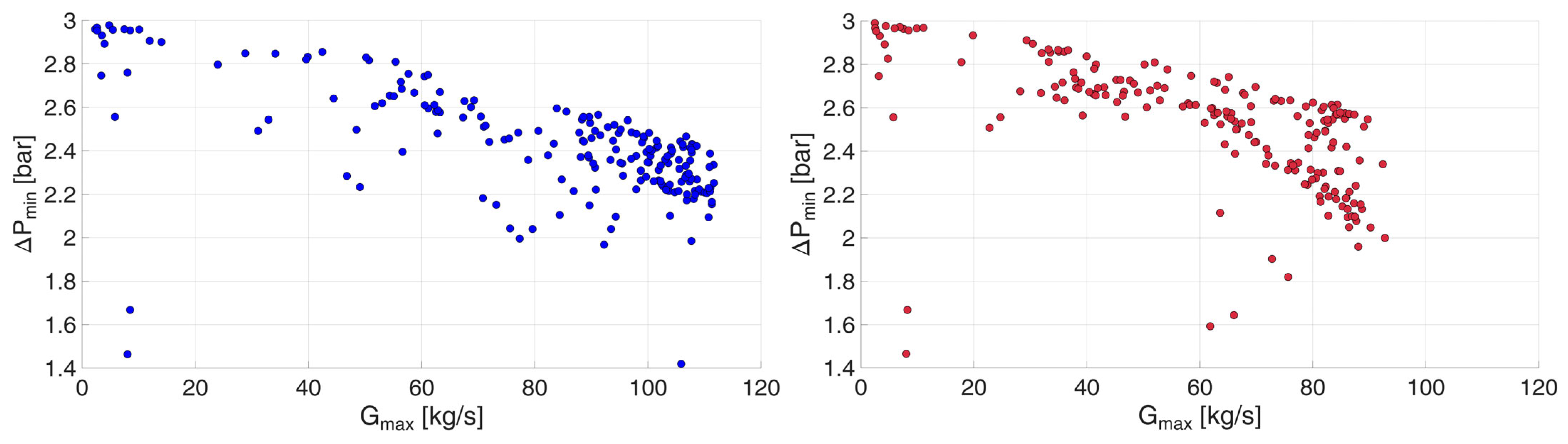
To assess how the peak flow reduction affects local hydraulic conditions, Figure 7 compares the minimum substation differential pressure at the daily network mass flow peak under current operation (blue) and with TDSM (red), keeping the plant differential pressure unchanged. In both scenarios, the results follow an approximately quadratic trend, with scatter reflecting differences in the spatial distribution of substation flows. Although TDSM reduces the aggregate network peak, the minimum differential pressure remains comparable to that under current operation. This reflects the nature of load shifting: it reduces the coincidence of substation peaks without reducing their individual magnitudes. Pressure losses along the paths supplying the hydraulically critical substations can therefore remain significant even when the total network flow decreases.

Figure 7. Substation differential pressures at the daily network mass flow peak under current operation ((left), blue) and with TDSM ((right), red), with the same differential pressure imposed at the plant.

4.2. Supply Temperature Reduction Enabled by TDSM

For the reference day, the peak reduction achieved through TDSM allows mass flow rates to increase by approximately 29% before the network peak reaches its original value. This additional flow compensates for the smaller temperature difference between supply and return, enabling lower supply temperatures while maintaining the same thermal power. Assuming that the return temperature remains unchanged, values between 55 and 65 °C yield supply temperatures of approximately 105–108 °C. This corresponds to a reduction of up to approximately 15 °C relative to the current supply temperature of 120 °C. This range represents an estimated hydraulic potential rather than a demonstrated operational set point. Since the reference day represents one of the most demanding operating conditions, this temperature reduction is expected to be feasible on most other days of the heating season. This expectation is subsequently verified by evaluating the differential pressures available at the substations under reduced-temperature operation.

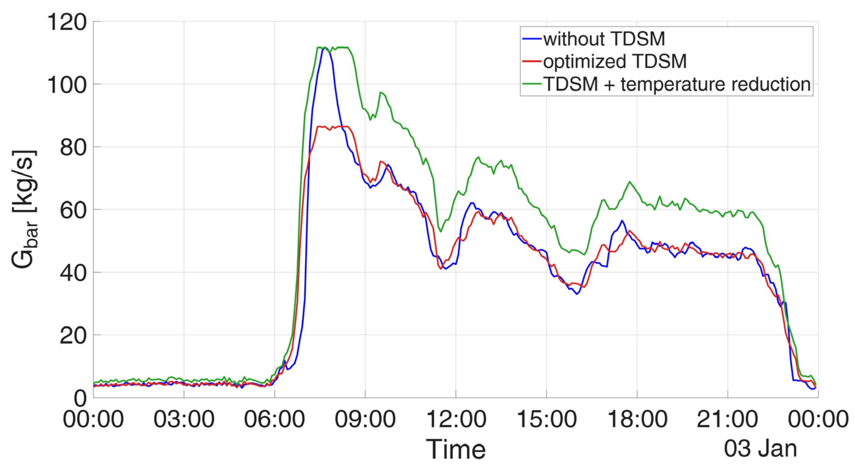
Figure 8 compares the mass flow rate profiles under current operation (blue), with TDSM at the current supply temperature (red), and with TDSM at reduced supply temperature (green). In the latter case, flow rates are increased until the peak matches that observed under current operation.

Figure 8. Reference-day mass flow rate profiles under current operation (blue), with TDSM (red), and with TDSM at reduced supply temperature (green), restoring the peak to its original value.

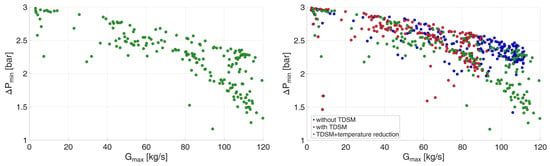
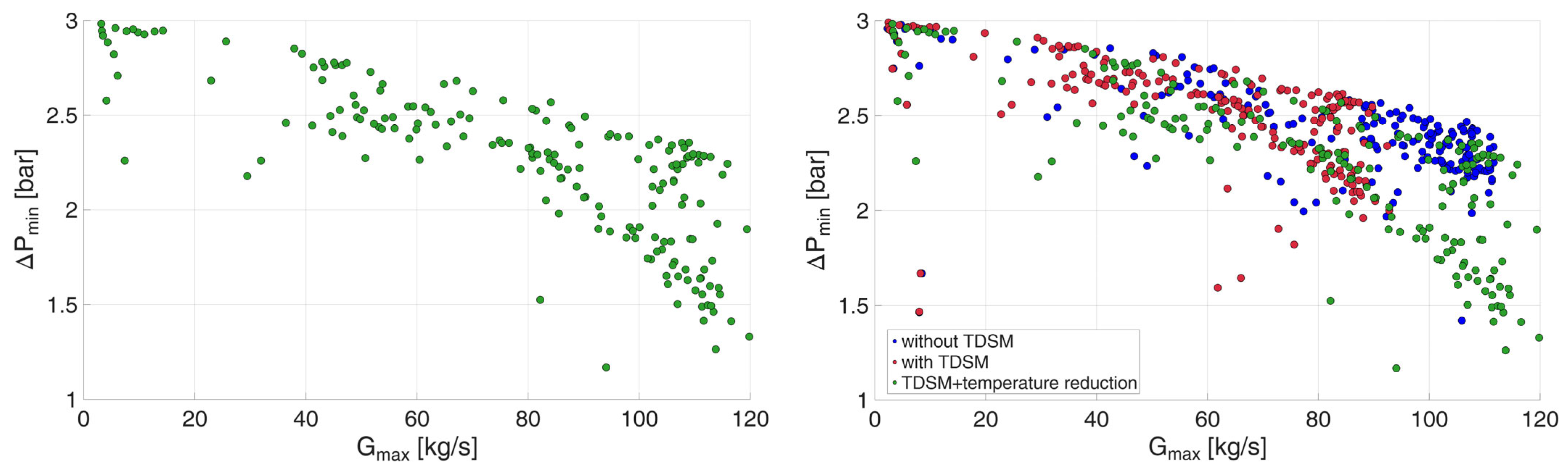
The hydraulic implications of reduced-temperature operation are assessed by evaluating the minimum substation differential pressure at the daily network mass flow peak for each day considered. Figure 9 presents these values in green in the left panel, while the right panel compares them with current operation (blue) and TDSM at the original supply temperature (red), keeping the plant differential pressure unchanged. The increased flow rates required at lower supply temperatures lead to higher pressure losses and lower minimum substation differential pressures, particularly on days with high network peaks. Although TDSM creates room for additional circulation by reducing the aggregate peak, restoring this peak to its original value does not necessarily restore the original pressure distribution, because the allocation of flows among substations also affects local hydraulic conditions. Nevertheless, the available differential pressures remain above 1.2 bar and are sufficient to sustain the required substation flow rates, supporting the hydraulic feasibility of the assessed supply temperature reduction despite the increased pressure losses. It should be noted that reducing the supply temperature requires higher flow rates and consequently greater pumping power. By reducing pressure losses, the TDSM strategy adopted here also aims to mitigate the associated increase in pumping costs, which will be quantified in future work.

Figure 9. Substation differential pressures at daily network mass flow peaks: reduced supply temperature with TDSM (left) and comparison of current operation ((right), blue), current supply temperature with TDSM ((right), red), and reduced supply temperature with TDSM ((right), green).

The assessment is then extended to individual substations, since compliance with network hydraulic constraints does not necessarily imply that every substation can accommodate a 29% increase in mass flow rate throughout the day. Substation flow constraints are assessed using operational data: the maximum mass flow rate recorded at each substation during the available heating season is adopted as its upper operating limit. This provides a conservative threshold, as the actual capacity may exceed the highest observed value. A detailed evaluation of substation thermal performance using a model such as that presented in [16] is reserved for future work.

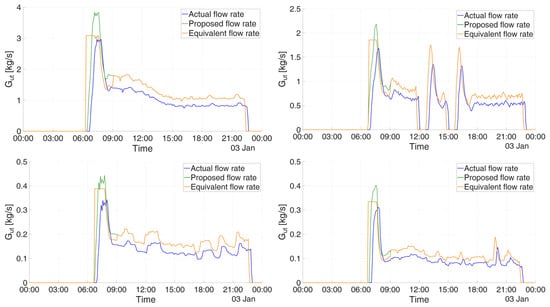
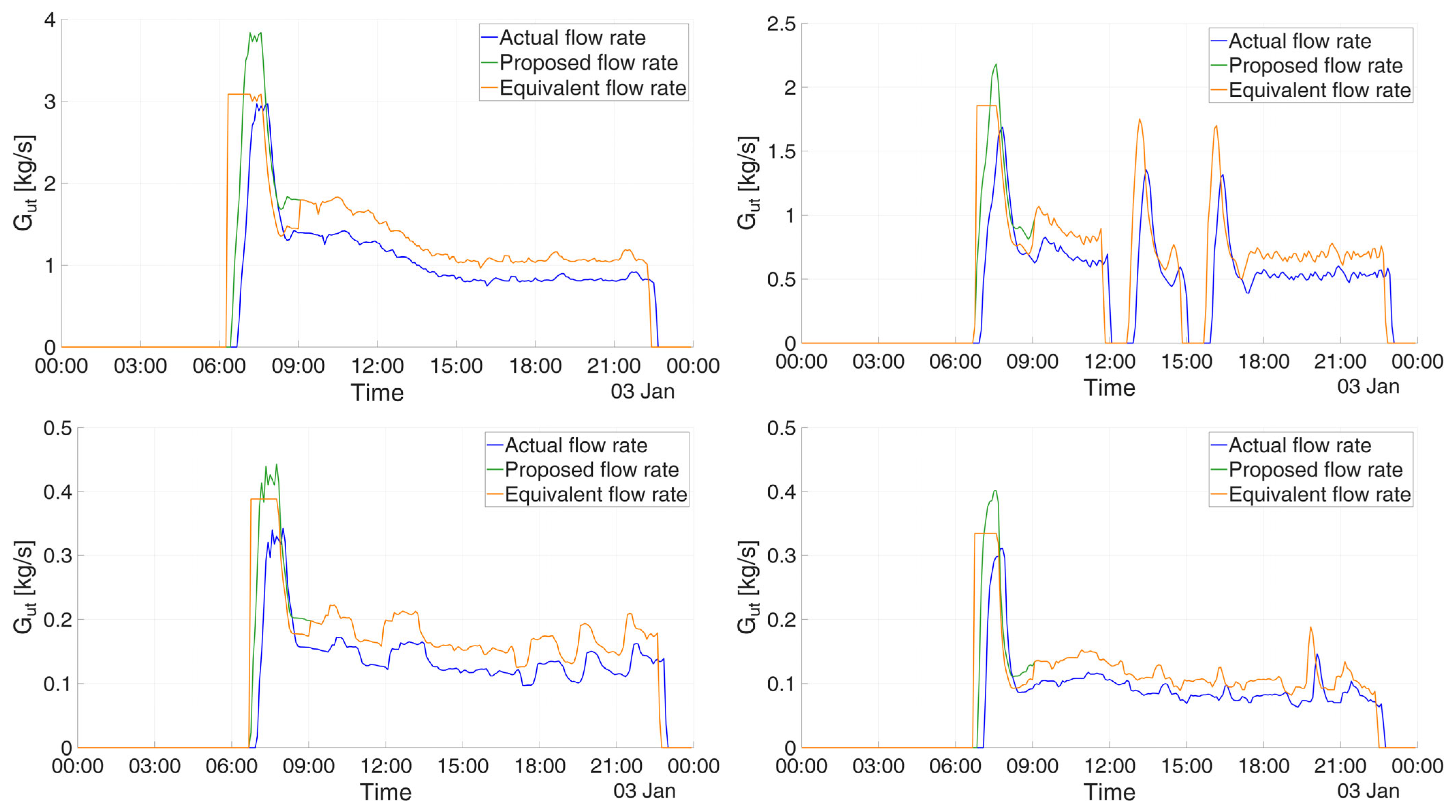
During the relatively steady afternoon operating period, the increased mass flow rates remain below these individual limits. During peak operation, however, the reduced-temperature profiles exceed the adopted thresholds at 12 substations on the analysed reference day. For these substations, the mass flow rate is capped, and heating operation is extended by advancing start-up to compensate for the reduction in thermal power and maintain the same total energy delivery. Unlike the load shifting described in Section 2.2, which translates the operating profile in time, this adjustment extends the duration of heating operation.

Figure 10 illustrates four of the 12 affected substations. The blue curves represent the original mass flow rate profiles, the green curves show the profiles increased by 29% for reduced temperature operation, and the orange curves represent the capped profiles with extended operation. This adjustment preserves the total thermal energy delivered under current operation while respecting the adopted substation flow limits. For the four substations shown, heating starts at approximately 06:45, around 40 min before the scheduled start-up time.

Figure 10. Mass flow rate profiles for four substations: current operation (blue), reduced-temperature operation with a 29% flow increase (green), and capped flows with extended heating operation to preserve total energy delivery (orange).

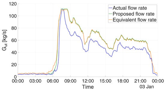
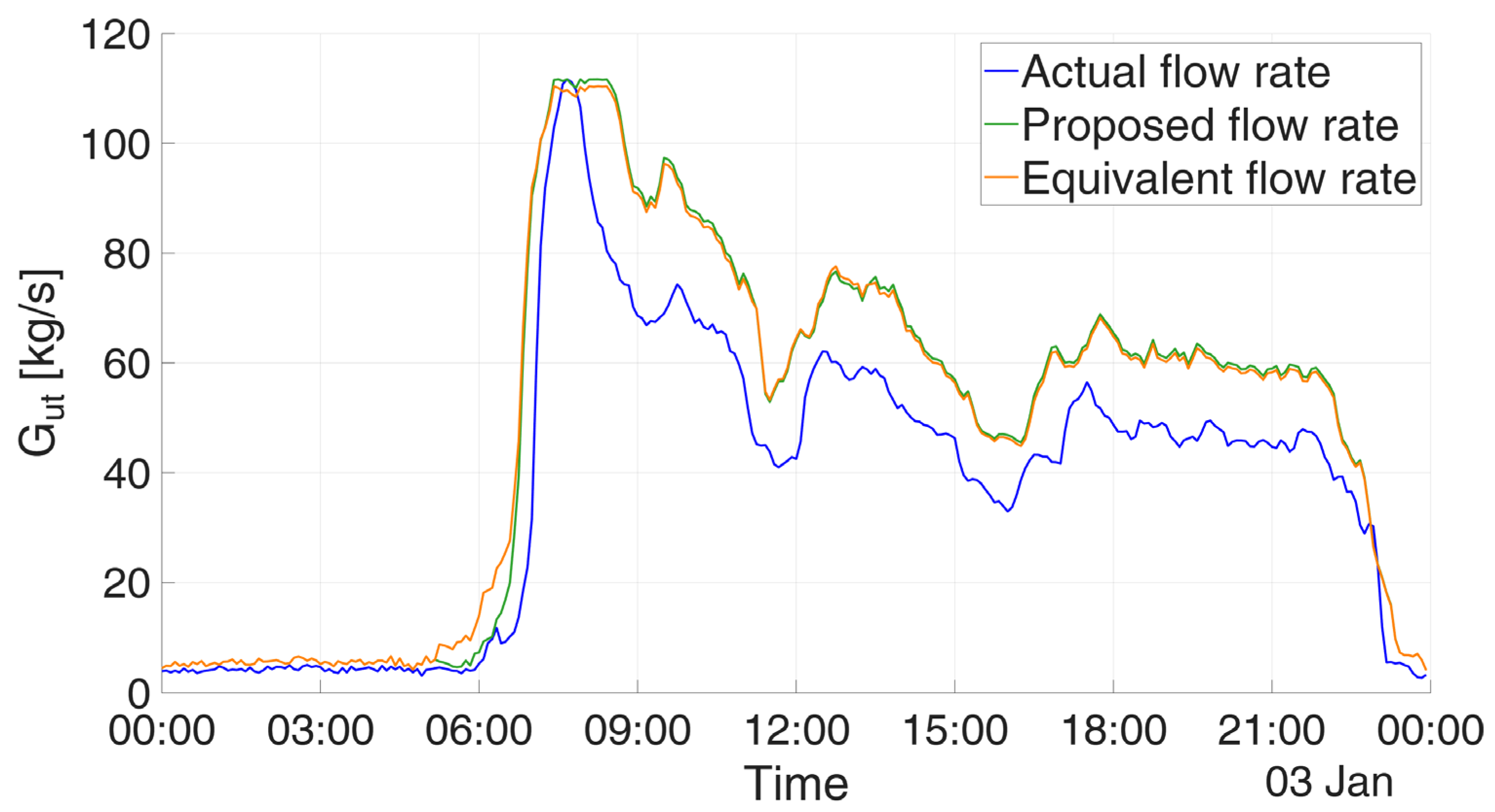
These adjustments are applied after optimization, without re-optimizing the schedule, and therefore do not alter the ±15 min constraint in the MILP, although the final operating profiles include these subsequent modifications. To verify that the additional advances have a limited impact on the aggregate mass-flow profile and that the modified schedules remain feasible, Figure 11 shows the total flow rate at the main node for the reference day after the start-up profiles of the affected substations were modified. The blue curve is the original flow rate profile, the green curve is the profile required to compensate for the reduced supply temperature, in which the flow rate is increased in inverse proportion to the temperature decrease, and the orange curve is the profile obtained after the start-up modifications. The orange curve never exceeds the maximum flow rate imposed at the main node and further reduces the aggregate peak flow by 1.15% relative to the profile before the additional advances.

Figure 11. Mass flow rate profiles for the main node: current operation (blue), reduced-temperature operation with a 29% flow increase (green), and capped flows with extended heating operation to preserve total energy delivery (orange).

The modifications therefore do not cause hydraulic problems in the network, and the modified schedules remain practically feasible. Moreover, the areas under the green and orange curves are identical. Since these areas represent the thermal energy delivered to the substations, which was constrained to remain unchanged, the procedure preserves the daily thermal energy delivery while respecting both the substation flow limits and the hydraulic limit of the network.

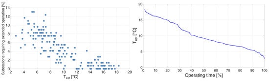
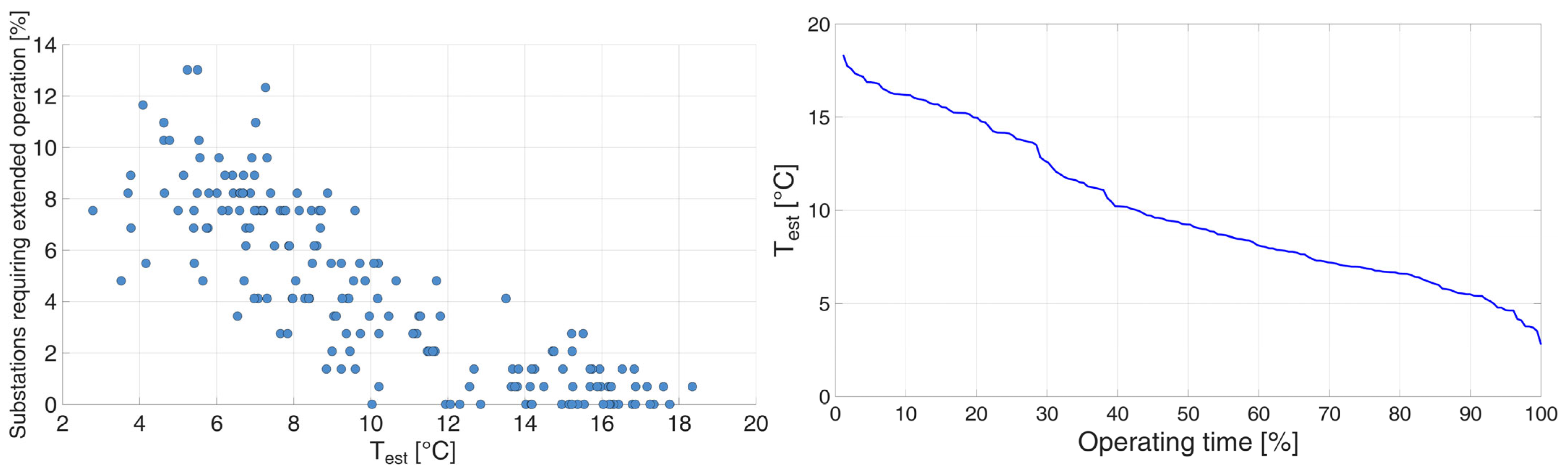
In general, only a small proportion of substations require extended heating operation, with the share remaining below approximately 13% on all days considered and generally decreasing as outdoor temperature rises (Figure 12, left). Moreover, the colder conditions associated with more frequent adjustments occur relatively rarely: outdoor temperatures below 6 °C account for less than 15% of the operating period (Figure 12, right).

Figure 12. Percentage of substations requiring extended heating operation as a function of outdoor temperature (left) and percentage of operating time during which each outdoor temperature is equal to or greater than a certain threshold (right).

These adjustments may further reduce the aggregate network peak relative to the uncapped profiles used in the preceding analysis. The resulting pressure losses could therefore be lower, leaving greater differential pressure available at the substations than previously estimated.

5. Conclusions

This study investigated how TDSM can enable sustainable supply temperature reduction in existing DH networks by creating hydraulic margin through peak flow reduction. The proposed methodology combines MILP optimization of substation start-up schedules, hydraulic simulations of the DH network, and a preliminary assessment of operation at reduced temperatures. Its application to a network serving 146 substations in northern Italy provides the following findings:

• Start-up shifts within ±15 min reduced the reference-day peak mass flow rate by 22.6%, from 111.7 to 86.4 kg/s. Applying the same schedule without further optimization also reduced daily peaks on all additional days assessed, demonstrating its effectiveness beyond the day used for optimization.
• This peak reduction allows an approximately 29% increase in mass flow rates relative to the TDSM profiles before the aggregate network peak returns to its original value. Assuming unchanged return temperatures between 55 and 65 °C, the estimated hydraulic potential corresponds to a supply temperature of about 105–108 °C, representing a reduction of up to approximately 12–15 °C. Across the days assessed, differential pressures evaluated at daily network peaks remained at or above the baseline minimum.
• Adopting historical maximum flows as conservative substation limits identified only 12 substations requiring adjustments on the reference cold day. Capping their flows and extending heating operation preserved total thermal energy delivery. Across all days considered, the proportion requiring such adjustments remained below approximately 13% and generally decreased with increasing outdoor temperature.

These results demonstrate a pathway for improving the sustainability of existing DH networks without requiring immediate large-scale infrastructure replacement. By reducing coincident start-up peaks, TDSM creates hydraulic capacity that can be used to lower supply temperatures while preserving daily thermal-energy delivery and baseline hydraulic performance. This operating change can increase the compatibility of existing networks with renewable and recovered heat sources that are available at lower temperature levels, thereby supporting their progressive integration into the heat supply. The proposed approach therefore identifies demand-side flexibility as an operational measure that can help existing high-temperature DH systems transition towards lower-temperature and more resource-efficient operation.

References

- International Energy Agency. Renewables 2021. Available online: https://www.iea.org/reports/renewables-2021 (accessed on 3 October 2026).
- Massulli, A.R.; Rosa, F.C.; Basso, G.L. Moving Towards Fourth-Generation District Heating as a Power-to-Heat Strategy: Techno-Economic Issues. Sustainability 2025, 17, 3675. [Google Scholar] [CrossRef] [Scilit]
- European Commission. An EU Strategy on Heating and Cooling; European Commission COM: Brussels, Belgium, 2016. [Google Scholar]
- Werner, S. International review of district heating and cooling. Energy 2017, 137, 617–631. [Google Scholar] [CrossRef] [Scilit]
- Connolly, D.; Lund, H.; Mathiesen, B.V.; Werner, S.; Möller, B.; Persson, U.; Boermans, T.; Trier, D.; Østergaard, P.A.; Nielsen, S. Heat Roadmap Europe: Combining district heating with heat savings to decarbonise the EU energy system. Energy Policy 2014, 65, 475–489. [Google Scholar] [CrossRef] [Scilit]
- International Energy Agency. 350 Million Building Units Connected to District Energy Networks by 2030, Provide About 20% of Space Heating Needs. Available online: https://www.iea.org/reports/350-million-building-units-connected-to-district-energy-networks-by-2030-provide-about-20-of-space-heating-needs (accessed on 4 October 2026).
- European Union. Directive (EU) 2023/1791 of the European Parliament and of the Council of 13 September 2023 on Energy Efficiency and Amending Regulation (EU) 2023/955 (Recast) (Text with EEA Relevance); European Union: Luxembourg, 2023. [Google Scholar]
- Mura, B.; Caputo, P.; Ferla, G. Decarbonization roadmap and compliance to Art. 26 of energy efficiency directive for an existing fossil fuelled district heating system. Energy Rep. 2025, 14, 5447–5459. [Google Scholar] [CrossRef] [Scilit]
- Caputo, P.; Ferla, G.; Mura, B.; Di Nunzio, N.C. Decarbonising Italy’s district heating and cooling sector: Drivers, barriers, and opportunities from stakeholder perspectives. Util. Policy 2026, 98, 102115. [Google Scholar] [CrossRef] [Scilit]
- Cowley, T.; Hutty, T.; Hammond, J.; Brown, S. Achieving emission reduction through the utilisation of local low-grade heat sources in district heating networks. Appl. Therm. Eng. 2024, 242, 122381. [Google Scholar] [CrossRef] [Scilit]
- Manz, P.; Billerbeck, A.; Kök, A.; Fallahnejad, M.; Fleiter, T.; Kranzl, L.; Braungardt, S.; Eichhammer, W. Spatial analysis of renewable and excess heat potentials for climate-neutral district heating in Europe. Renew. Energy 2024, 224, 120111. [Google Scholar] [CrossRef] [Scilit]
- Dorca, A.; Sarbu, I. Hybridisation of District Heating in Existing Office Buildings Using Air-to-Water Heat Pumps: A Case Study on Energy and Performance. Sustainability 2026, 18, 4965. [Google Scholar] [CrossRef] [Scilit]
- Averfalk, H.; Ingvarsson, P.; Persson, U.; Gong, M.; Werner, S. Large heat pumps in Swedish district heating systems. Renew. Sustain. Energy Rev. 2017, 79, 1275–1284. [Google Scholar] [CrossRef] [Scilit]
- Pastore, L.M. Sector Coupling and Flexibility Measures in Distributed Renewable Energy Systems: A Comprehensive Review. Sustainability 2026, 18, 437. [Google Scholar] [CrossRef] [Scilit]
- Ancona, M.A.; Branchini, L.; De Pascale, A.; Melino, F. Smart District Heating: Distributed Generation Systems’ Effects on the Network. Energy Procedia 2015, 75, 1208–1213. [Google Scholar] [CrossRef] [Scilit]
- Bonelli, G.; Capone, M.; Verda, V.; Guelpa, E. Modeling and Performance Evaluation of a District Heating Network with Integration of a Thermal Prosumer: A Case Study in Italy. Energies 2025, 18, 5977. [Google Scholar] [CrossRef] [Scilit]
- Testasecca, T.; Catrini, P.; Beccali, M.; Piacentino, A. Dynamic simulation of a 4th generation district heating network with the presence of prosumers. Energy Convers. Manag. X 2023, 20, 100480. [Google Scholar] [CrossRef] [Scilit]
- Sipilä, K. Cogeneration, biomass, waste to energy and industrial waste heat for district heating. In Advanced District Heating and Cooling (DHC) Systems; Woodhead Publishing: Oxford, UK, 2015; pp. 45–73. [Google Scholar] [CrossRef] [Scilit]
- Socci, L.; Leoncini, L.; Zini, A.; Mazzoni, S.; Rocchetti, A. Data Centre Waste Heat for Building Heating: A Comparative Energy Analysis in Italy. Sustainability 2026, 18, 6061. [Google Scholar] [CrossRef] [Scilit]
- Verzino, A.; Talluri, L.; Rocchetti, A.; Socci, L. Smart Reuse of Waste Heat from Data Centres: Energy and Exergy Analysis for a District-Heating Network in Bulgaria. Energies 2026, 19, 800. [Google Scholar] [CrossRef] [Scilit]
- Slatina, I.; Biloglav, A.; Čehil, M.; Schneider, D.R.; Soldo, V. Enhancing the energy and environmental performance of third-generation district heating systems via wastewater heat integration. Energy 2026, 361, 142178. [Google Scholar] [CrossRef] [Scilit]
- Lagoeiro, H.; Maidment, G.; Ziemele, J. Potential of treated wastewater as an energy source for district heating: Incorporating social elements into a multi-factorial comparative assessment for cities. Energy 2024, 304, 132190. [Google Scholar] [CrossRef] [Scilit]
- Kljajić, M.V.; Anđelković, A.S.; Hasik, V.; Munćan, V.M.; Bilec, M. Shallow geothermal energy integration in district heating system: An example from Serbia. Renew. Energy 2020, 147, 2791–2800. [Google Scholar] [CrossRef] [Scilit]
- Zajacs, A.; Shogenova, A.; Shogenov, K.; Volkova, A.; Sliaupa, S.; Sliaupiene, R.; Jõeleht, A. Utilization of Geothermal Energy: New Possibilities for District Heating Networks in the Baltic States. Renew. Energy 2025, 242, 122375. [Google Scholar] [CrossRef] [Scilit]
- Lindenberger, D.; Bruckner, T.; Groscurth, H.M.; Kümmel, R. Optimization of solar district heating systems: Seasonal storage, heat pumps, and cogeneration. Energy 2000, 25, 591–608. [Google Scholar] [CrossRef] [Scilit]
- Frison, L.; Kollmar, M.; Oliva, A.; Bürger, A.; Diehl, M. Model predictive control of bidirectional heat transfer in prosumer-based solar district heating networks. Appl. Energy 2024, 358, 122617. [Google Scholar] [CrossRef] [Scilit]
- Dalla Rosa, A.; Li, H.; Svendsen, S.; Werner, S.; Persson, U.; Ruehling, K.; Felsmann, C.; Crane, M.; Burzynski, R.; Bevilacqua, C. Toward 4th Generation District Heating: Experience and Potential of Low-Temperature District Heating—IEA DHC Annex X Report; Technical University of Denmark: Kongens Lyngby, Denmark, 2014; Available online: https://orbit.dtu.dk/en/publications/iea-dhc-annex-x-reporttoward-4th-generation-district-heating-expe/ (accessed on 10 October 2026).
- Averfalk, H.; Benakopoulos, T.; Best, I.; Dammel, F.; Engel, C.; Geyer, R.; Gudmundsson, O.; Lygnerud, K.; Nord, N.; Oltmanns, J.; et al. Low-temperature District Heating Implementation Guidebook—Final Report of IEA DHC Annex TS2. In Proceedings of the Technology Collaboration Programme by IEA, online, 26–28 October 2021. [Google Scholar]
- Cenian, A.; Dzierzgowski, M.; Pietrzykowski, B. On the road to low temperature district heating. J. Phys. Conf. Ser. 2019, 1398, 012002. [Google Scholar] [CrossRef] [Scilit]
- Dzierzgowski, M.; Cenian, A. District heating in Lomża—How a polish city responded to EU energy measures towards decarbonisation of economy. Energy 2026, 356, 138242. [Google Scholar] [CrossRef] [Scilit]
- Merlet, Y.; Baviere, R.; Vasset, N. Optimal retrofit of district heating network to lower temperature levels. Energy 2023, 282, 128386. [Google Scholar] [CrossRef] [Scilit]
- Capone, M.; Guelpa, E.; Verda, V. Potential for supply temperature reduction of existing district heating substations. Energy 2023, 285, 128597. [Google Scholar] [CrossRef] [Scilit]
- Hietaharju, P.; Ruusunen, M. Peak Load Cutting in District Heating Network. In Proceedings of The 9th EUROSIM Congress on Modelling and Simulation, EUROSIM 2016, The 57th SIMS Conference on Simulation and Modelling SIMS 2016; Linköping University Electronic Press: Linköping, Sweden, 2018; Volume 142, pp. 99–104. [Google Scholar] [CrossRef] [Scilit]
- Arnaudo, M.; Topel, M.; Puerto, P.; Widl, E.; Laumert, B. Heat demand peak shaving in urban integrated energy systems by demand side management—A techno-economic and environmental approach. Energy 2019, 186, 115887. [Google Scholar] [CrossRef] [Scilit]
- Saletti, C.; Gambarotta, A.; Morini, M. Development, analysis and application of a predictive controller to a small-scale district heating system. Appl. Therm. Eng. 2020, 165, 114558. [Google Scholar] [CrossRef] [Scilit]
- Guelpa, E.; Mutani, G.; Todeschi, V.; Verda, V. Reduction of CO2 emissions in urban areas through optimal expansion of existing district heating networks. J. Clean. Prod. 2018, 204, 117–129. [Google Scholar] [CrossRef] [Scilit]
- Li, H.; Wang, S.J. Load Management in District Heating Operation. Energy Procedia 2015, 75, 1202–1207. [Google Scholar] [CrossRef] [Scilit]
- Cai, H.; Ziras, C.; You, S.; Li, R.; Honoré, K.; Bindner, H.W. Demand side management in urban district heating networks. Appl. Energy 2018, 230, 506–518. [Google Scholar] [CrossRef] [Scilit]
- Wernstedt, F.; Davidsson, P.; Johansson, C. Demand side management in district heating systems. In Proceedings of the International Conference on Autonomous Agents, Honolulu, HI, USA, 14–18 May 2007; pp. 1383–1389. [Google Scholar] [CrossRef] [Scilit]
- Patankar, S.V.; Spalding, D.B. A calculation procedure for heat, mass and momentum transfer in three-dimensional parabolic flows. Int. J. Heat Mass Transf. 1972, 15, 1787–1806. [Google Scholar] [CrossRef] [Scilit]
- Guelpa, E.; Toro, C.; Sciacovelli, A.; Melli, R.; Sciubba, E.; Verda, V. Optimal operation of large district heating networks through fast fluid-dynamic simulation. Energy 2016, 102, 586–595. [Google Scholar] [CrossRef] [Scilit]
- Capone, M. Physical Model of District Heating Networks to Boost the Transition to Next-Generation Systems. Math. Model. Eng. Probl. 2025, 12, 3427–3434. [Google Scholar] [CrossRef] [Scilit]
- Bezanson, J.; Edelman, A.; Karpinski, S.; Shah, V.B. Julia: A fresh approach to numerical computing. SIAM Rev. 2017, 59, 65–98. [Google Scholar] [CrossRef] [Scilit]
- Gurobi Optimization. Gurobi Optimizer Reference Manual. Available online: https://www.gurobi.com (accessed on 7 September 2026).
- Capone, M.; Canino, M.; Guelpa, E. Dynamic temperature supply to boost the integration of renewable energy into existing district heating networks. Renew. Energy 2026, 256, 124315. [Google Scholar] [CrossRef] [Scilit]
Disclaimer/Publisher’s Note: The statements, opinions and data contained in all publications are solely those of the individual author(s) and contributor(s) and not of MDPI and/or the editor(s). MDPI and/or the editor(s) disclaim responsibility for any injury to people or property resulting from any ideas, methods, instructions or products referred to in the content. |
© 2026 by the authors. Licensee MDPI, Basel, Switzerland. This article is an open access article distributed under the terms and conditions of the Creative Commons Attribution (CC BY) license.