


Abstract
This study develops a composite risk index (CRI) to assess flood vulnerability in Mueang Maha Sarakham District, northeastern Thailand, by integrating four sub-indices into the CRI—the Net Economic Loss Index (NELI), Income Loss Sensitivity Index (ILSI), Adaptation Cost Index (ACI), and Community Economic Resilience Index (CERI)—with the Maladaptive Development Risk Index (MDRI) reported separately as a contextual factor. The CRI was constructed from 63,017 grid points (approximately 100-m sampling resolution) covering approximately 1236 km2, with elevations ranging from 129 to 203 m. Risk classes were defined using a tertile split of the CRI distribution (20th and 80th percentiles), yielding three approximately balanced classes: Low (20.0%, n = 12,604), Moderate (60.0%, n = 37,809), and High (20.0%, n = 12,604). Spatial clustering (k = 4) identified four distinct risk profiles: Low Risk (32.5%), Moderate Risk (33.0%), Resilient (22.6%), and High Risk (11.9%). Out-of-sample testing against the temporally separated 2025 flood occurrence yielded an area under the receiver operating characteristic curve (AUC) of 0.771 for the CRI, with individual indices achieving AUCs of 0.910 (NELI), 0.844 (ILSI), 0.891 (ACI), 0.816 (CERI, after inversion), and 0.838 (MDRI). The association between risk class and flood occurrence was significant (Cramér’s V = 0.2381, p < 0.001), with the High-risk class containing 993 of the 1077 flooded points. Random Forest (RF) models using spatial block cross-validation achieved AUC-ROC (area under the receiver operating characteristic curve) values of 0.999 (Model A: indices only) and 0.999 (Model B: indices + physical), with AUC-PR (area under the precision–recall curve) of 0.295 and 0.766, respectively. SHapley Additive exPlanations (SHAP) analysis identified mndwi_2024 (Modified Normalized Difference Water Index for 2024), DEM (Digital Elevation Model), flood_freq (flood frequency), and NELI as the most influential predictors. Because Flood_2025 captures flood occurrence rather than consequence severity, these AUC values validate the indices’ association with flood exposure, not their validity as measures of flood consequences. Direct validation of consequence-related performance would require household-level data on economic loss, recovery time, and displacement, which were unavailable in this study. The framework provides a transferable approach for data-scarce regions, but its interpretation should be limited to flood-exposure assessment.
1. Introduction
1.1. Background and Problem Statement
Climate change has intensified hydrological extremes globally, with floods becoming more frequent, prolonged, and intense [1,2]. Southeast Asia, particularly the Lower Mekong Basin, is among the most flood-prone regions worldwide [3,4]. Thailand’s Chi River Basin exemplifies these challenges, experiencing recurrent monsoon floods that threaten livelihoods, infrastructure, and sustainable development [5,6]. Large flood events in Thailand, such as the 2011 Chao Phraya River flood, illustrate the national-scale economic and social consequences of recurrent flooding [7,8], and highlight the need for systematic risk assessment frameworks [9].
Traditional flood risk assessment has focused on physical exposure—flood frequency, depth, and extent—often overlooking socioeconomic vulnerability [10,11]. While valuable for hazard characterization, these approaches fail to capture communities’ differential capacity to anticipate, absorb, and recover from flood impacts [12,13]. This limitation is critical in agricultural floodplains where livelihood strategies, income sources, and social networks fundamentally determine household resilience [14,15].
A more fundamental issue, however, has received insufficient attention: the distinction between drivers of flood OCCURRENCE and modulators of flood CONSEQUENCES. Physical factors (elevation, topography, antecedent moisture) determine whether flooding occurs at a given location. Socioeconomic factors (income diversity, social capital, adaptive capacity) determine how severely communities suffer when flooding occurs. Conflating these two dimensions leads to circular reasoning, where indices constructed to measure vulnerability are then used to predict vulnerability itself. This circularity has been identified as a critical methodological weakness in numerous composite index studies [16,17], and the validation of social vulnerability indices against independent outcomes remains particularly challenging [18], yet few studies have explicitly addressed it.
Recent advances in remote sensing and geographic information systems (GIS) enable systematic flood monitoring [19,20], while machine learning methods such as Random Forest (RF) and Extreme Gradient Boosting (XGBoost) capture complex relationships between environmental variables and flood occurrence [21,22,23]. Studies in the Chi River Basin have advanced flood hazard assessment, including the identification of a critical elevation threshold (~150 m) controlling flood intensity [24] and the demonstration of temporal generalization challenges in flood prediction [25]. Related work in the region has also developed integrated hydro-hazard indices for drought-flood risk assessment [26]. Broader reviews of composite index construction have repeatedly flagged circular validation—the use of index components as both predictors and targets—as a critical methodological weakness [27,28]. Very few studies, however, have explicitly tested composite indices against temporally separated outcomes.
Despite these advances, three critical gaps remain:
No established framework distinguishes between the drivers of flood occurrence and the modulators of flood consequences in a single integrated assessment.
Circular validation is prevalent in composite index studies, where indices are used as both predictors and targets.
Community typologies based on vulnerability and resilience profiles remain unexplored despite the recognition that place-based community resilience models are essential for understanding disaster impacts [29], limiting differentiated risk management strategies.
1.2. The Need for Novel Composite Indices
Vulnerability has evolved from a narrow focus on physical exposure to a multidimensional understanding encompassing economic, social, and institutional dimensions [21,22]. However, operationalizing this understanding remains challenging [24,25]. Existing approaches suffer from four limitations: (1) fragmented measurement—vulnerability dimensions assessed in isolation [26,27]; (2) limited spatial integration—assessments at coarse administrative scales that do not align with decision-making units [28,29]; (3) absence of community typology—treating communities as homogeneous [30,31]; and (4) limited operationalization of resilience—few practical indicators for operational flood risk management [32,33].
To address these gaps, this study introduces four novel composite indices and a Composite Risk Index:
Net Economic Loss Index (NELI): Quantifies the gap between actual flood losses and compensation received. Based on previous research documenting that compensation covers only 14.24% of total damages in the Chi River Basin [34], NELI captures the financial burden that accumulates over repeated flood events, potentially creating poverty traps [35], and increasing the risk of maladaptation as households are forced into unsustainable coping strategies [36].
Income Loss Sensitivity Index (ILSI): Measures household income sensitivity to flood disruption [37]. ILSI captures the vulnerability of households dependent on daily wages, agriculture, or informal employment—livelihood strategies particularly susceptible to flood impacts [14,15,34].
Adaptation Cost Index (ACI): Quantifies the financial burden of flood protection measures—home elevation, structural reinforcement, and other adaptive investments [38]. ACI captures both households’ capacity to adapt and residual vulnerability.
Community Economic Resilience Index (CERI): Measures communities’ capacity to anticipate, absorb, and recover from flood shocks [39,40]. CERI integrates social networks, community cohesion, resource access, and environmental quality [41].
Composite Risk Index (CRI): Integrates NELI, ILSI, ACI, and CERI into a single comprehensive measure, enabling classification of communities into risk levels.
Note on Maladaptive Development Risk Index (MDRI). Our original conceptualization included MDRI (capturing development patterns that increase vulnerability) as a fifth CRI component. However, the Random Forest analysis in Section 3.5 revealed that adding MDRI as a predictor did not improve predictive performance for the 2025 flood outcome (AUC-PR decreased from 0.766 in Model B to 0.750 in Model C). We therefore report MDRI separately as a contextual factor rather than integrating it into the CRI. The final CRI equation (Equation (13)) includes only four components: NELI, ILSI, ACI, and CERI.
1.3. Research Objectives and Questions
This study addresses identified gaps with four objectives:
Objective 1: Develop four novel composite indices (NELI, ILSI, ACI, CERI) and a Composite Risk Index (CRI) capturing the multidimensional nature of flood vulnerability.
Objective 2: Distinguish between drivers of flood occurrence (physical exposure) and modulators of flood consequences (socioeconomic vulnerability) using temporally separated validation.
Objective 3: Identify distinct community typologies based on vulnerability and resilience profiles using CERI-weighted K-means clustering.
Objective 4: Provide evidence-based policy recommendations for sustainable flood risk management, contributing to the Sustainable Development Goals (SDGs) 11, 13, and 15.
Four research questions guide this study, each addressed in a specific section:
RQ1: What are the statistical properties and distributions of the four novel composite indices and the CRI? (addressed in Section 3.1 and Section 3.2)
RQ2: Do socioeconomic vulnerability indices predict flood occurrence, or do they primarily modulate flood consequences? (addressed in Section 3.4 and Section 3.5)
RQ3: What critical thresholds and non-linear relationships characterize flood occurrence determinants? (addressed in Section 3.6)
RQ4: What distinct community typologies emerge based on vulnerability and resilience profiles? (addressed in Section 3.7)
1.4. Significance and Contributions
Theoretical contributions: This study advances vulnerability theory by demonstrating the fundamental distinction between drivers of flood occurrence and modulators of flood consequences. We show that socioeconomic vulnerability, while important for consequences, has limited predictive power for occurrence in the Chi River floodplain.
Methodological contributions: Four novel composite indices provide a replicable framework for integrated vulnerability assessment. We demonstrate an honest validation framework using temporally separated outcomes, avoiding the circularity that plagues many composite index studies. The spatial block cross-validation design (5 km × 5 km grid) further ensures that model performance is not inflated by spatial autocorrelation.
Practical contributions: Elevation-based zoning (Red < 145 m, Yellow 145–155 m, Green > 155 m) provides actionable land use regulation. Four community types (Low Risk, Resilient, Moderate Risk, High Risk) enable differentiated management. SHAP-derived thresholds provide descriptive (not causal) intervention criteria.
Policy contributions: This study contributes directly to SDGs 11 (Sustainable Cities and Communities), 13 (Climate Action), and 15 (Life on Land) by providing evidence-based tools for sustainable flood risk management.
1.5. Paper Structure
2. Materials and Methods
2.1. Study Area
This study was conducted in the Upper Chi River Basin within Mueang Maha Sarakham District, Maha Sarakham Province, northeastern Thailand (16°06′ N, 103°18′ E; 16.1055° N, 103.3060° E). The study area covers approximately 1236 km2 of low-relief terrain (elevation: 129–203 m above mean sea level). The elevation range was verified directly from the 5 m resolution DEM used in the analysis; earlier reports of 130–226 m were based on a coarser regional DEM and have been corrected in this revision. The region has a tropical savanna climate (Köppen Aw) with a distinct wet season (May–October, 1200–1500 mm rainfall) and dry season (November–April). Agriculture dominates land use (80.1%), primarily rain-fed rice paddies, with forest patches along river corridors. The area experiences recurrent flooding, with major events in 2018, 2021, 2022, and 2025 [1,2].
The study area was selected because it represents a typical low-relief tropical floodplain in the Lower Mekong Basin, where the interaction between monsoon hydrology and intensive rice agriculture creates recurrent flood risk. The area is also representative of other floodplain environments in northeastern Thailand and Laos, where similar topographic and socioeconomic conditions prevail.
2.2. Data Sources and Processing
A point-based sampling framework of 63,017 spatial points was generated using stratified random sampling across land use types, elevation zones, and flood exposure history [3,4]. The spatial resolution of the sampling framework was approximately 100 m, which is sufficient to capture the topographic and land use gradients that control flood exposure in this low-relief floodplain.
2.2.1. Flood Data and Spatial Distribution
Flood occurrence data were obtained from the Department of Disaster Prevention and Mitigation (DDPM), Thailand, for four years: 2017, 2018, 2021, and 2022. Flood presence was recorded as binary (1 = flood occurred, 0 = no flood) and validated using Sentinel-1 Synthetic Aperture Radar (SAR) imagery (European Space Agency, Paris, France; overall accuracy: 87–93%) [5,6]. The 2025 flood data (1077 points, 1.7%) were deliberately excluded from all index construction and used exclusively as an independent validation outcome. This temporal separation is the cornerstone of our validation framework: it ensures that the CRI is tested against an outcome that was not used in its construction, thereby avoiding the circularity that has plagued previous composite index studies.
As shown in Figure 1c–f, the spatial distribution of flood events varies considerably across years. The 2018 flood affected 7348 points (11.7%), representing the most extensive event. The 2022 flood affected 5514 points (8.8%), while the 2017 flood affected 5499 points (8.7%). The 2021 flood was the smallest event, affecting only 2273 points (3.6%).
Figure 1.
Spatial distribution of annual flood events in Mueang Maha Sarakham District, northeastern Thailand (2017–2025). (a) Flood points for 2017 (5499 points). (b) Flood points for 2018 (7348 points). (c) Flood points for 2021 (2273 points). (d) Flood points for 2022 (5514 points). (e) Flood points for 2025 (1077 points). (f) Location map of Maha Sarakham Province in northeastern Thailand, showing the study area boundary and the Chi River network. In panels (a–e), red dots indicate flooded points and grey dots indicate non-flooded sampling points. Flood events are concentrated along the Chi River corridor and in low-lying areas below 145 m elevation. Note: The spatial extent of the 2025 flood (panel (e)) is smaller and located in the northern part of the study area, which is consistent with the lower number of flooded points (1077) compared to other years.
Two flood metrics were derived from the flood data. First, flood frequency (flood_freq) was calculated as the sum of flood events across the observation years [Equation (1)]:
flood_freq = Flood2017 + Flood2018 + Flood2021 + Flood2022
Second, flood cumulative impact (flood_cumulative) was calculated using temporal weights to reflect the increasing relevance of recent events [Equation (2)]:
flood_cumulative = (Flood2017 × 0.1) + (Flood2018 × 0.2) + (Flood2021 × 0.3) + (Flood2022 × 0.4)
The 2025 flood event (Flood_2025) was treated separately as a binary outcome variable (1 = flooded in 2025, 0 = not flooded in 2025) and was not included in either flood_freq or flood_cumulative.
The 63,017-point dataset was partitioned into training and test sets using a spatially blocked design (5 km × 5 km grid). Grid cells were assigned to either training or testing, so that spatially proximate points never appeared in both sets. This design prevents spatial autocorrelation from inflating model performance. The resulting training set contained 47,963 points (76.1%) and the test set contained 15,054 points (23.9%), which is consistent with the confusion-matrix counts reported in Section 3.5. The often-cited figure of 20,000 points refers to an earlier random split that was discarded in favour of the spatially blocked design.
2.2.2. Land Use Data and Transitions
Land use data were obtained for 2015, 2018, and 2023 from Sentinel-2 imagery (European Space Agency, Paris, France) at 10 m resolution [10]. Classification was performed in Google Earth Engine (version 1.4.0; Google LLC, Mountain View, CA, USA), with overall accuracy of 89.2% and Kappa of 0.87 [42]. Four categories were used: Agriculture (1), Forest (2), Urban (3), and Water (4).
As shown in Figure 2d, Agriculture was the dominant land use across all years, declining from 85.9% in 2015 to 80.1% in 2023, while Urban areas increased from 10.6% to 12.6%. Forest cover fluctuated between 1.5% (2015) and 3.2% (2023), and Water bodies increased from 2.0% (2015) to 4.3% (2023). These transitions were summarized into seven types (Table 1): Stable (86.1%), Urbanization (4.6%), Urban to Agriculture (2.6%), Agriculture to Forest (2.2%), Deforestation (0.6%), Water to Agriculture (0.5%), and Other (0.2%).
Figure 2.
Land use composition and spatial distribution in Mueang Maha Sarakham District (2015–2023). (a–c) Spatial distribution maps showing the geographic patterns of Agriculture (green), Forest (dark green), Urban (red), and Water (blue) for the years 2015, 2018, and 2023, respectively. Grey areas represent non-sampled points. (d–f) Pie charts showing the percentage composition of each land use type (Agriculture, Forest, Urban, and Water) for the years 2015, 2018, and 2023, respectively. The legend for the pie charts is provided in panel (c), and the numerical percentages are displayed directly on each chart. Note: The spatial distribution maps (a–c) show a consistent pattern across all years, where Agriculture dominates the landscape, covering over 80% of the study area. The slight increase in Urban and Water areas in 2023 is accurately reflected in the corresponding pie chart (f).
Table 1.
Land use transitions (2015–2023).
2.2.3. Remote Sensing Spectral Indices
Spectral indices were derived from Sentinel-2 imagery (2020, 2023, 2024) at 10-m resolution during the dry season (January–May) [44]. Four indices were calculated [11,12,13,14,15]: the Normalized Difference Vegetation Index (NDVI) [45,46], Modified Normalized Difference Water Index (MNDWI) [30], Vegetation Condition Index (VCI) [31], and Normalized Difference Moisture Index (NDMI). The MNDWI formulation follows Gao [47], and the VCI formulation follows Kogan [48].
NDVI = (NIR − Red)/(NIR + Red)
MNDWI = (Green − SWIR)/(Green + SWIR)
VCI = ((NDVI − NDVI_min)/(NDVI_max − NDVI_min)) × 100
NDMI = (NIR − SWIR)/(NIR + SWIR)
2.2.4. Topographic Variables
Topographic variables were derived from a 5 m resolution Digital Elevation Model (DEM): elevation (DEM), slope, Topographic Wetness Index (TWI) [Equation (7)] [18,19,20,21], and proximity to streams (prox2stream) [22]. The TWI formulation follows the standard contributing-area approach [49,50]. The TWI was calculated in Python (version 3.11; Google Colab, Google LLC, Mountain View, CA, USA) using the numpy (version 1.26.0) and rasterio (version 1.3.9) libraries, following Equation (7):
where α is the local upslope area contributing to a given point (m2 m−1) and β is the local slope angle (radians).
TWI = ln(α/tan β)
2.2.5. Socioeconomic Proxy Construction
Household-level socioeconomic data (occupation, income, housing quality, social capital, and recovery capacity) were not available at the point level. We therefore constructed spatial proxies from land use, spectral indices, and topographic variables. The full provenance of each proxy—including the input variables, the weighting scheme, and the source of the assigned values—is documented in Appendix A (Table A1), and the rationale for each proxy is summarised below.
Occupation proxy (occ_proxy). Derived from the 2023 land use classification. Each land use class was assigned an occupation-risk value reflecting the relative income sensitivity of the dominant occupation type to flood disruption: Agriculture → 0.7, Urban → 0.5, Water → 0.9, Forest → 0.2. The assignment follows the livelihood-vulnerability literature for rural Southeast Asia, in which agricultural and informal water-dependent livelihoods are consistently more sensitive to flood disruption than formal urban employment [34,35].
Income risk proxy (Inc_Risk). Weighted combination of land use (70%) and NDVI 2024 (30%). Lower NDVI indicates lower agricultural productivity and therefore higher income risk. The 70/30 weighting reflects the dominance of agricultural income in the study area and the secondary role of vegetation condition as a productivity signal [43,46].
Housing quality proxy (Hous_Risk). Derived from land use classification: Urban → 0.1 (good), Agriculture → 0.4 (moderate), Water/Forest → 0.8 (poor). These values reflect the association between urban land use and permanent construction materials, and between water-adjacent or forest land use and temporary or semi-permanent housing [36].
Dependency risk proxy (Dep_Risk). Weighted combination of VCI 2024 (40%) [48], Inc_Risk (30%), and land use (30%). This proxy captures the degree to which household income depends on flood-sensitive production [34,35,43]. Duration risk proxy (Dur_Risk). Weighted combination of TWI (60%) and DEM (40%). This proxy captures the duration of waterlogging during flood events, with higher TWI and lower DEM indicating longer inundation.
Protection cost proxy (Prot_Cost_Risk). Derived from land use classification: Agriculture → 0.7 (high investment capacity required), Urban → 0.3 (lower cost due to infrastructure), Water/Forest → 0.5 (moderate). The values reflect the relative cost of structural adaptation in each land-use class [36].
Social capital proxy (Social_Capital). Weighted combination of land use (40%), NDVI 2024 (30%), and proximity to streams (30%). Areas with mixed land use, higher vegetation, and proximity to water sources are assumed to have stronger social networks, following the community-resilience literature [41,51].
Recovery capacity proxy (Recovery_Capacity). Weighted combination of flood frequency (40%), NDVI 2024 (30%), and land use (30%). Areas with lower flood frequency and higher vegetation are assumed to have higher recovery capacity.
Because household-level data were unavailable, these proxies are indirect measures of socioeconomic conditions and may not fully capture household-level heterogeneity. This limitation is discussed in Section 4.7.
2.3. Composite Index Construction
2.3.1. Net Economic Loss Index (NELI)
NELI quantifies the gap between actual flood losses and compensation received [17], calculated as:
NELI = (Direct_Damage + Indirect_Damage) − Compensation
Direct damage was calculated as land use value × (1 + flood_freq_norm) × 1.3. Indirect damage was calculated as daily income × flood duration × 0.7. Compensation was set at 14.24% of total damages [34]. Values were normalized to 0–1.
2.3.2. Income Loss Sensitivity Index (ILSI)
ILSI measures household income sensitivity to flood disruption [18]:
where Occ_Risk = occupation risk, Dep_Risk = dependency risk, Dur_Risk = duration risk, and Inc_Risk = income risk. The weights (0.35, 0.25, 0.25, 0.15) were derived from the previous literature on livelihood vulnerability [14,15,35] and reflect the relative importance of each dimension in determining income sensitivity.
ILSI = (Occ_Risk × 0.35) + (Dep_Risk × 0.25) + (Dur_Risk × 0.25) + (Inc_Risk × 0.15)
2.3.3. Adaptation Cost Index (ACI)
ACI quantifies flood protection costs [19]:
where Prox_Risk = proximity risk (<200 m: 1.0; 200–500 m: 0.7; 500–800 m: 0.4; >800 m: 0.2), Hous_Risk = housing risk (Good: 0.1; Moderate: 0.4; Poor: 0.8), and Prot_Cost_Risk = protection cost risk. The weights were adjusted from the original 0.35/0.25/0.20/0.25 to 0.40/0.30/0.30 after removing Freq_Risk (which overlapped with flood_freq used separately in the RF model) to avoid double counting.
ACI = (Prox_Risk × 0.40) + (Hous_Risk × 0.30) + (Prot_Cost_Risk × 0.30)
2.3.4. Community Economic Resilience Index (CERI)
CERI measures community adaptive capacity [20,21]:
where Social_Capital = social capital proxy, Env_Quality = environmental quality (NDVI), and Recovery_Capacity = recovery capacity proxy. The weights were derived from the previous literature on community resilience [41,51,52].
CERI = (Social_Capital × 0.40) + (Env_Quality × 0.35) + (Recovery_Capacity × 0.25)
2.3.5. Maladaptive Development Risk Index (MDRI)
MDRI captures development patterns that increase vulnerability [36,53]:
where LU_Change = land use change risk (Agriculture/Forest → Urban: 1.0; Deforestation: 0.6), Pop_Growth = population growth risk (applies when growth > 5%), and Env_Deg = environmental degradation. The weights were adjusted from the original 0.35/0.20/0.15/0.25 to 0.50/0.30/0.20 after removing Flood_Change to avoid double counting with flood_freq.
MDRI = (LU_Change × 0.50) + (Pop_Growth × 0.30) + (Env_Deg × 0.20)
2.3.6. Composite Risk Index (CRI) and Threshold Determination
CRI integrates the four indices into a single risk measure [23]:
CRI = (NELI × 0.30) + (ILSI × 0.25) + (ACI × 0.25) + ((1 − CERI) × 0.20)
The weights (0.30, 0.25, 0.25, 0.20) were derived from a combination of literature review and expert judgment. NELI receives the highest weight (0.30) because it captures the direct economic burden of flooding, which is the most immediate determinant of household vulnerability in the Chi River floodplain. ILSI and ACI receive equal weights (0.25 each) because income sensitivity and adaptation cost represent complementary dimensions of economic vulnerability. CERI receives the lowest weight (0.20) because it captures the protective dimension of resilience, which moderates but does not directly determine flood risk. MDRI is reported separately as a contextual factor rather than integrated into the CRI, because sensitivity analysis revealed that it did not improve predictive performance (AUC-PR decreased from 0.766 to 0.750 when included).
Risk class definition. Risk classes were defined using a tertile split of the CRI distribution, with the 20th and 80th percentiles as cut-points. This yielded three approximately balanced classes: Low Risk (n = 12,604; 20.0%), Moderate Risk (n = 37,809; 60.0%), and High Risk (n = 12,604; 20.0%). This tertile split follows the baseline weighting scheme described in Equation (13). These thresholds are consistent with previous flood risk classification studies in Southeast Asia [7,18] and were validated through sensitivity analysis (Section 3.2).
Risk levels: Low (CRI ≤ 20th percentile), Moderate (20th–80th percentile), High (CRI > 80th percentile).
These tertiles produce three classes: Low Risk (20.0%, n = 12,604), Moderate Risk (60.0%, n = 37,809), and High Risk (20.0%, n = 12,604).
2.4. Machine Learning Framework
2.4.1. Random Forest Classification
Two Random Forest classifiers were trained using scikit-learn (version 1.4.0; scikit-learn developers, open-source) [54] under a spatially blocked train–test split (5 km × 5 km grid). The spatial split assigns entire grid cells to either training or testing, so that spatially proximate points never appear in both sets. This design prevents spatial autocorrelation from inflating model performance [21,28]. The split produced a training set of 47,963 points (76.1% of the 63,017-point dataset) and a test set of 15,054 points (23.9%), the latter matching the confusion-matrix counts reported in Section 3.5.
Classifier 1: CRI-derived risk classes (three-class). The first classifier predicted the CRI-derived risk classes (Low, Moderate, High) obtained by applying the CRI thresholds defined in Section 2.3.6. This classifier evaluates how consistently the composite indices reproduce the intended risk typology and provides the confusion matrices reported in Section 3.5. Because the target classes are constructed from the same indices used as predictors, this classifier functions as a consistency check on the index construction rather than as independent validation.
Classifier 2: Flood_2025 (binary, independent). The second classifier predicted the temporally separated 2025 flood outcome (1 = flooded in 2025, 0 = not flooded in 2025). This outcome was withheld from all index construction and from the calculation of flood_freq, and therefore provides an independent test of whether the predictors carry genuine information about flood occurrence. This classifier is the basis for the AUC and AUC-PR values reported in Section 3.5 and for the SHAP analysis in Section 3.6. Flood_2025 was never used as a predictor in either classifier.
Four predictor configurations were evaluated for the binary classifier predicting Flood_2025:
Model A: Socioeconomic indices only (NELI, ILSI, ACI, CERI).
Model B: Socioeconomic indices plus physical/environmental variables (DEM, Slope, TWI, Prox2streamlines, flood_freq, Flood_2018, ndvi_2024, mndwi_2024).
Model C: All variables including MDRI (as an additional predictor, not as a CRI component).
Model D: Physical/environmental variables only (to test whether socioeconomic indices add incremental predictive value beyond physical exposure).
The predictor set consisted of thirteen variables: NELI, ILSI, ACI, CERI, MDRI, DEM, Slope, TWI, Prox2streamlines, flood_freq, Flood_2018, ndvi_2024, and mndwi_2024. Model A used four predictors, Model B used twelve, and Model C used thirteen.
Two clarifications on predictor construction are necessary. First, Flood_2017–2025 was not included as a single predictor; instead, the year 2018 was retained as a separate binary predictor (Flood_2018) and flood_freq served as a cumulative measure over the 2017–2022 observation window. The year 2025 was excluded entirely: it was not included in flood_freq, flood_cumulative, or the predictor set of either classifier. Second, flood_cumulative was excluded from the final models because it was highly correlated with flood_freq (r > 0.95) and did not improve predictive performance, thereby avoiding double counting of the same underlying flood-exposure information
2.4.2. Model Evaluation
Performance was evaluated using accuracy [Equation (14)], precision [Equation (15)], recall [Equation (16)], F1-score [Equation (17)], and AUC [28], following standard statistical evaluation procedures [55]:
where TP = true positive, TN = true negative, FP = false positive, and FN = false negative.
Accuracy = (TP + TN)/(TP + TN + FP + FN)
Precision = TP/(TP + FP)
Recall = TP/(TP + FN)
F1 = 2 × (Precision × Recall)/(Precision + Recall)
2.4.3. SHAP Analysis
SHAP (SHapley Additive exPlanations) was performed using TreeExplainer in the SHAP Python library (version 0.44.0; SHAP developers, open-source) [56]. SHAP values decompose each prediction:
where φ0 is the base value, φj is the SHAP value for feature j, and M is the number of features. The SHAP values represent the contribution of each feature to the prediction for a given instance, and the mean absolute SHAP value represents the global importance of each feature.
f(x) = φ0 + Σj=1ᴹ φj
2.4.4. Feature Importance
Feature importance was extracted as the mean decrease in impurity [24]:
where T is the number of trees, S is the set of splits using feature j, and ΔI(s) is the impurity decrease at split s.
Importancej = (1/T) Σt=1ᵀ Σs ∈ S ΔI(s)
2.5. Spatial and Statistical Analysis
Principal Component Analysis (PCA) was performed on standardized variables using scikit-learn (version 1.4.0; scikit-learn developers, open-source) [57]. K-means clustering [58] was performed using scikit-learn (version 1.4.0; scikit-learn developers, open-source) to identify community typologies [30], with the optimal cluster number determined by the elbow method and silhouette score using the following variables: NELI, ILSI, ACI, CERI, MDRI, flood_freq, DEM, and ndvi_2024. Spatial autocorrelation was assessed using Moran’s I [59] implemented in PySAL (version 2.6.0; PySAL developers, open-source) or GeoDa (version 1.20.0; University of Chicago, Chicago, IL, USA). The Moran’s I value for the CRI was 0.42 (p < 0.001), indicating significant spatial clustering of flood risk. This spatial autocorrelation motivated the use of spatial block cross-validation in the Random Forest analysis. The overall analytical workflow is summarised in Figure 3. The framework proceeds from data acquisition (flood inventory, land use, spectral indices, and topography) through socioeconomic proxy construction, composite index development, and weight sensitivity analysis. Two analytical tracks then run in parallel: independent validation against the temporally separated 2025 flood event, and spatially blocked Random Forest classification of flood occurrence. These are followed by SHAP interpretation, Principal Component Analysis, and CERI-weighted K-means clustering, which together inform the dual-track policy framework presented in Section 4.6.
Figure 3.
Overall research framework. The workflow proceeds from data acquisition (flood inventory, land use, spectral indices, topography) through socioeconomic proxy construction, composite index development, weight sensitivity analysis, independent validation against Flood_2025, spatial Random Forest classification, SHAP interpretation, and K-means clustering.
3. Results
3.1. Descriptive Statistics of the Composite Indices
The six composite indices exhibited distinct distributional characteristics (Table 2). The Net Economic Loss Index (NELI) showed the widest range (0.0000–1.0000) with a mean of 0.5000 (SD = 0.2887). The Income Loss Sensitivity Index (ILSI) had a mean of 0.5203 (SD = 0.0646), with values concentrated toward the middle of the scale (Q1 = 0.4768, median = 0.5217, Q3 = 0.5691). The Adaptation Cost Index (ACI) exhibited a mean of 0.4679 (SD = 0.0860). The Community Economic Resilience Index (CERI) showed a mean value of 0.6051 (SD = 0.0793). The Maladaptive Development Risk Index (MDRI) had a mean of 0.5000 (SD = 0.2887). The Composite Risk Index (CRI) yielded a mean of 0.4760 (SD = 0.1140) with a range of 0.2110–0.7365, confirming substantial spatial heterogeneity in overall flood risk.
Table 2.
Descriptive statistics of composite indices (n = 63,017).
Figure 4 displays the probability density distributions of all six indices by risk level. Risk classes were defined using a tertile split: Low Risk (n = 12,604; 20.0%), Moderate Risk (n = 37,809; 60.0%), and High Risk (n = 12,604; 20.0%). NELI shows the widest range (0.0000–1.0000) with clear separation across risk classes, while CERI exhibits the highest overall mean (0.6051) and a reverse gradient (highest in Low Risk, lowest in High Risk).
Figure 4.
Violin plots of six composite indices by risk level (n = 63,017): (a) NELI, (b) ILSI, (c) ACI, (d) CERI, (e) MDRI, and (f) CRI. Red dashed lines indicate mean values, and black horizontal lines inside boxes indicate medians. Risk classes were defined using a tertile split of the CRI distribution at the 20th and 80th percentiles: Low Risk (CRI ≤ 20th percentile; n = 12,604; 20.0%), Moderate Risk (20th–80th percentile; n = 37,809; 60.0%), and High Risk (CRI > 80th percentile; n = 12,604; 20.0%). NELI shows the widest range (0.0000–1.0000) with clear separation across risk classes, while CERI exhibits the highest overall mean (0.6051) and a reverse gradient (highest in Low Risk, lowest in High Risk).
3.2. Flood Inventory and Spatial Distribution
The final analytical dataset comprised 63,017 georeferenced spatial points distributed across the Upper Chi River Basin within Mueang Maha Sarakham District, Maha Sarakham Province, northeastern Thailand. Elevation across the sampled points ranged from 129 to 203 m above mean sea level, with the majority of observations concentrated in the low-relief floodplain below 160 m. Land use in 2023 was dominated by agriculture (80.1%), followed by urban areas (12.6%), water bodies (4.3%), and forest (3.0%).
Flood occurrence data from the Department of Disaster Prevention and Mitigation (DDPM) recorded four major events during the 2017–2022 observation window. Table 3 presents the annual flood statistics. The 2018 and 2022 events were the most severe, affecting 7348 points (11.7%) and 5514 points (8.8%) respectively, while the 2021 event affected only 2273 points (3.6%). The 2017 event affected 5499 points (8.7%). The 2025 event, although more recent, affected only 1077 points (1.7%). Across the 2017–2022 window, 20,634 points (32.8%) experienced at least one flood event. The cumulative flood frequency (flood_freq) therefore ranged from 0 to 4 events, with a mean of 0.33 and a standard deviation of 0.72—values that are used directly as a predictor in the Random Forest model described in Section 3.5. The 2025 flood event was deliberately withheld from the calculation of flood_freq and from all stages of index construction, and was retained exclusively as an independent validation outcome.
Table 3.
Annual flood statistics (2017–2025).
The spatial distribution of these events is shown in Figure 5. Flood frequency is highest along the Chi River corridor and in areas below approximately 145 m, where flood frequencies of two or more events are common. This pattern provides an initial indication of the topographic control on flood exposure that is examined formally in Section 3.7.
Figure 5.
Spatial distribution of flood frequency and severity across Mueang Maha Sarakham District. (a) Flood frequency map showing the cumulative number of flood events (2017–2022) per point, ranging from 0 to 4 events. (b) Flood severity distribution by year, showing the percentage of points affected annually. The Chi River corridor (red) shows the highest flood frequency, with 2018 and 2022 identified as the most severe flood years. Areas with elevations below 145 m exhibit flood frequencies ≥ 2 events, confirming the topographic control on flood exposure.
The Spearman correlation matrix (Figure 6), following standard correlation analysis [59], revealed that CRI was most strongly correlated with NELI (ρ = 0.758) and MDRI (ρ = 0.515), followed by ACI (ρ = 0.458) and ILSI (ρ = 0.320). CERI showed a weak negative correlation with CRI (ρ = −0.069), consistent with its interpretation as a protective factor. Notably, MDRI exhibited negative correlations with ILSI (ρ = −0.354) and CERI (ρ = −0.376), suggesting that maladaptive development patterns are associated with lower income sensitivity and lower community resilience—a pattern consistent with urbanizing areas where formal employment reduces income sensitivity but social cohesion may be weaker.
Figure 6.
Spearman correlation matrix of the six composite indices. CRI was most strongly correlated with NELI (ρ = 0.758) and MDRI (ρ = 0.515), followed by ACI (ρ = 0.458) and ILSI (ρ = 0.320). CERI showed a weak negative correlation with CRI (ρ = −0.069), consistent with its interpretation as a protective factor. MDRI exhibited negative correlations with ILSI (ρ = −0.354) and CERI (ρ = −0.376).
Distinctiveness of the Composite Indices
To assess whether the four component indices provide distinct information, we examined their pairwise Spearman correlations and their individual AUC values against Flood_2025.
Pairwise correlations. NELI and CERI were weakly correlated (ρ = 0.266), and NELI and ACI were moderately correlated (ρ = 0.349). ILSI showed only weak correlations with the other indices (ρ = 0.006–0.160), indicating that income sensitivity is largely orthogonal to the other dimensions. CERI was negatively correlated with MDRI (ρ = −0.376), consistent with the interpretation that maladaptive development erodes community resilience.
Independent AUC values against Flood_2025. NELI achieved the highest AUC (0.910), followed by ACI (0.891), ILSI (0.844), and MDRI (0.838). CERI showed an AUC of 0.184, which after inversion (1 − AUC = 0.816) reflects its interpretation as a protective resilience index. CRI achieved the highest overall AUC (0.939). These differences indicate that the indices are not equally informative for predicting flood occurrence.
Double counting. Flood frequency enters ACI, CERI, and MDRI. To avoid double counting with the separate flood_freq predictor in the Random Forest model, we removed Freq_Risk from ACI (Section 2.3.3) and Flood_Change from MDRI (Section 2.3.5). Flood_cumulative was excluded from the Random Forest predictors because it was highly correlated with flood_freq (r > 0.95).
Formal redundancy test. A formal variance-inflation analysis was not performed because the indices are used as separate predictors in the Random Forest models rather than as a single linear combination. However, the low pairwise correlations and the divergent AUC values indicate that the indices capture distinguishable dimensions. The comparison with a simpler vulnerability measure (e.g., a single income-based index) remains a direction for future work.
3.3. Sensitivity of the CRI to Weight Perturbation
To assess whether the CRI classification was robust to the subjective weighting scheme (Figure 7), a Monte Carlo weight perturbation analysis was conducted (n = 500 iterations, ±30% random perturbation of all weights). The mean classification agreement with the baseline CRI was 0.946, with the 5th percentile agreement at 0.897. The mean Spearman rank correlation between perturbed and baseline CRI values was 0.9919, indicating that the ordinal ranking of locations was highly stable. Alternative weight schemes (equal weights, vulnerability-heavy, resilience-heavy, economic-heavy, adaptation-heavy, and MDRI-heavy) all yielded Cohen’s κ ≥ 0.6 relative to the baseline classification, with the minimum κ across schemes at 0.667 and the maximum at 1.000. These results confirm that the CRI classification is not an artifact of the chosen weights and remains stable under reasonable alternative weighting assumptions.
Figure 7.
Weight sensitivity analysis. (a) Monte Carlo agreement distribution (n = 500) with mean agreement of 0.946 and 90% agreement threshold at 0.90. (b) Rank correlation distribution with mean Spearman ρ of 0.9919. (c) Alternative weight scheme comparison showing Cohen’s κ for each scheme, with the 0.8 threshold indicating strong agreement.
3.4. Out-of-Sample Test Against the 2025 Flood Occurrence
To address the circularity inherent in using CRI components as predictors of CRI-derived classes, the indices were tested against an independent outcome: the observed 2025 flood event, which was excluded from all index construction. The CRI achieved an out-of-sample AUC of 0.771 for predicting Flood_2025, with an average precision of 0.0340 and a Cramér’s V of 0.2381 (p < 0.001). Among the individual indices, NELI achieved the highest in-sample AUC (0.910), followed by ACI (0.891), ILSI (0.844), MDRI (0.838), and CERI (0.816 after inversion). The in-sample single-index AUC for CRI was 0.939, while the out-of-sample AUC was 0.771 (Figure 8). When CRI was tested against multiple independent outcomes, it achieved the highest AUC for flood_2025 (AUC = 0.771), while its performance for vci_deficit was weakest (AUC = 0.469).
Figure 8.
Independent validation against the 2025 flood event. (a) Receiver operating characteristic (ROC) curves for predicting Flood_2025, with NELI achieving the highest AUC (0.910), followed by ILSI (0.844), CERI (0.816), and CRI (0.771). The dashed diagonal line represents random classification (AUC = 0.5). (b) AUC comparison across multiple independent outcomes, showing that CRI achieves the highest AUC for flood_2025 (0.771), followed by vci_deficit (0.469), ndvi_drop (0.543), and composite (0.547). The black dashed vertical line at 0.5 indicates the random baseline, while the orange (0.7) and red (0.8) dashed vertical lines indicate moderate and strong AUC thresholds, respectively.
These results indicate that the composite indices—particularly NELI, ILSI, and CERI—carry genuine predictive information about a temporally separated flood occurrence, providing external validation against an occurrence outcome. Because Flood_2025 records whether flooding occurred rather than how severe the consequences were, this test does not validate the indices as measures of consequence severity. However, the relatively low Spearman correlation between CRI and Flood_2025 (ρ = 0.122) suggests that the relationship is primarily driven by the binary classification threshold rather than a monotonic rank relationship, and this limitation is discussed further in Section 4.7.
Testing Against Additional Independent Outcomes
To assess whether the composite indices carry information beyond the binary 2025 flood outcome, we tested them against three additional independent outcomes derived from remote sensing and land use data: vegetation-condition deficit (vci_deficit), NDVI drop (ndvi_drop), and a composite impact indicator.
VCI deficit. The 2024 Vegetation Condition Index was compared against the long-term VCI baseline. Points with negative VCI anomaly were classified as having a vegetation-condition deficit. CRI achieved an AUC of 0.469, which is close to random, indicating that the CRI carries little information about vegetation-condition deficit.
NDVI drop. The difference between NDVI 2024 and NDVI 2020 was used to identify points with a substantial decline in vegetation cover. CRI achieved an AUC of 0.543, again close to random.
Composite impact indicator. A composite indicator combining flood frequency and vegetation-condition deficit was constructed. CRI achieved an AUC of 0.547.
These results indicate that the CRI’s predictive information is specific to the flood outcome and does not generalise to vegetation-condition or composite impact measures. This is consistent with the interpretation that the CRI captures flood-specific vulnerability rather than general environmental stress. However, we acknowledge that vegetation-condition and NDVI-based outcomes are indirect proxies for economic loss and displacement, and that direct measurements of economic loss, recovery time, and displacement would provide a stronger test of consequence-related validity. The current validation is therefore limited to flood occurrence, not flood consequences. Future research should collect such data through household surveys.
3.5. Spatial Random Forest Classification and Feature Importance
Two Random Forest classifiers were trained under the spatially blocked split described in Section 2.4.1: one predicting CRI-derived risk classes (Low, Moderate, High) and one predicting the independent binary Flood_2025 outcome.
Classification of CRI-derived risk classes. The three-class classifier reproduced the CRI typology with high accuracy. The normalized confusion matrix (Figure 9a) shows per-class accuracy of 98.3% for Low Risk, 96.6% for Moderate Risk, and 97.1% for High Risk. The absolute confusion matrix (Figure 9b) gives the corresponding counts: 4607 Low Risk, 8345 Moderate Risk, and 1679 High Risk points correctly classified (test set n = 15,054). Misclassification was confined to adjacent classes: 154 Moderate Risk points were classified as High Risk and 137 as Low Risk, while no Low Risk point was classified as High Risk and no High Risk point as Low Risk. This pattern indicates that the classifier preserves the ordinal structure of the risk typology. Because the target classes are constructed from the same indices that serve as predictors, this result should be read as a consistency check on the index construction rather than as independent validation.Prediction of Flood_2025. The binary classifier predicting the independent 2025 flood outcome is summarised in Table 4. Four predictor configurations were evaluated under the spatially blocked split. Model A used only the four socioeconomic indices that enter the CRI (NELI, ILSI, ACI, CERI) and achieved AUC-ROC = 0.9926 and AUC-PR = 0.2952. Model B added the eight physical and environmental variables (DEM, Slope, TWI, Prox2streamlines, flood_freq, Flood_2018, ndvi_2024, mndwi_2024) and achieved AUC-ROC = 0.9989 and AUC-PR = 0.7657. Model C added MDRI as an additional predictor and achieved AUC-ROC = 0.9990 and AUC-PR = 0.7499. Model D used only the eight physical and environmental variables and achieved AUC-PR = 0.7499 (AUC-ROC not retained; see Table 4 note). The baseline positive rate in the test set was 0.0141. Three conclusions follow. First, the large gain in AUC-PR from Model A to Model B (0.2952 → 0.7657) shows that physical and environmental variables add substantial discriminative information beyond the socioeconomic indices alone. Second, comparing Model D (physical only, AUC-PR = 0.7499) with Model B (physical + socioeconomic, AUC-PR = 0.7657) shows that adding the four socioeconomic indices yields a small but positive improvement in predictive performance for flood occurrence (Δ AUC-PR = +0.0158). This result indicates that socioeconomic indices carry incremental information about flood occurrence beyond physical exposure alone, although the gain is modest relative to the contribution of physical variables. Third, the comparison between Model B and Model C shows that adding MDRI as a predictor slightly reduces performance (AUC-PR = 0.7657 → 0.7499), supporting the decision to report MDRI separately rather than integrating it into the CRI.
Figure 9.
Normalized and absolute confusion matrices for the spatial split. (a) Normalized confusion matrix showing 98.3% accuracy for Low Risk, 96.6% for Moderate Risk, and 97.1% for High Risk. (b) Absolute confusion matrix showing the number of points in each category.
Table 4.
Random Forest performance for predicting the independent Flood_2025 outcome under spatial block cross-validation.
Under spatial block cross-validation (32 blocks), the Random Forest model achieved an AUC-ROC of 0.9989 (Model B, Table 4). This confirms that the spatially blocked design does not inflate performance and that the reported metrics are honest with respect to spatial autocorrelation.
The Random Forest feature importance ranking for the Flood_2025 classifier (Model B) is shown in Figure 10. Mndwi_2024 was the single most important predictor (importance = 0.148), followed by flood_freq (0.128), NELI (0.107), ndvi_2024 (0.105), CERI (0.088), ILSI (0.083), TWI (0.078), Slope (0.065), DEM (0.064), Flood_2018 (0.056), Prox2streamlines (0.048), and ACI (0.042). When grouped by category, physical and environmental variables collectively accounted for 68.2% of total importance, while socioeconomic indices accounted for 31.8%. Because MDRI is not included in Model B, its contribution is 0.0% in this model. This distribution indicates that physical exposure and socioeconomic vulnerability contribute comparably to the prediction of flood occurrence, with physical variables slightly dominant. The relatively high ranking of NELI (0.107) and CERI (0.088) among the socioeconomic indices suggests that economic vulnerability does influence flood outcomes, but through pathways that are distinct from the physical drivers of occurrence.Precision-recall and ROC curves for all four configurations are shown in Figure 11.
Figure 10.
Random Forest feature importance for predicting Flood_2025 (Model B). (a) Bar chart of predictors ranked by importance, with mndwi_2024, flood_freq, and NELI ranking highest. (b) Pie chart by category showing the relative contribution of physical/environmental (68.2%) vs. socioeconomic (31.8%) variables.
Figure 11.
ROC and Precision-Recall curves for predicting Flood_2025 under spatial block cross-validation. (a) Precision–Recall curves: Model A (average precision, AP = 0.295), Model B (AP = 0.766), Model C (AP = 0.750), Model D (AP = 0.750). Baseline positive rate = 0.0141 (test set). (b) ROC curves: Model A (AUC = 0.993), Model B (AUC = 0.999), Model C (AUC = 0.999), Model D (dotted line; AUC-ROC not retained in the spatial block cross-validation output). The dashed diagonal line represents random classification. Model definitions are provided in Section 2.4.1.
3.6. SHAP Analysis of Flood Occurrence Drivers
To interpret the binary Flood_2025 classifier (Classifier 2 in Section 2.4.1) and identify the direction and magnitude of each predictor’s contribution to flood occurrence, SHAP analysis was performed on Model B using TreeExplainer. The mean absolute SHAP values (Figure 12) ranked mndwi_2024 as the most influential feature (mean |SHAP| = 0.1065), followed by DEM (0.0907), flood_freq (0.0702), NELI (0.0418), ACI (0.0405), Flood_2018 (0.0392), ILSI (0.0322), ndvi_2024 (0.0277), CERI (0.0252), Prox2streamlines (0.0176), Slope (0.0160), and TWI (0.0126). The three highest-ranked features are all physical or environmental variables, and the summed SHAP contribution of physical variables (0.3805) substantially exceeds that of the socioeconomic indices (0.1397). By category, socioeconomic indices account for 31.8% of SHAP importance and physical/environmental variables for 68.2%. The test AUC-PR for Model B is 0.7657.
Figure 12.
SHAP feature importance (mean |SHAP|). The three highest-ranked features are all physical or environmental variables, with mndwi_2024, DEM, and flood_freq dominating the prediction of flood occurrence. Socioeconomic indices (NELI, ACI, ILSI, CERI) rank 4th, 5th, 7th, and 9th, respectively.
The beeswarm summary plot (Figure 13) shows the direction of each effect. High values of mndwi_2024 are associated with strongly positive SHAP values, indicating that surface moisture increases the probability of flooding. Low DEM values are associated with positive SHAP values, confirming that lower elevations face higher flood probability. High flood_freq values produce positive SHAP contributions, while high CERI values produce negative contributions, consistent with the protective role of community resilience.
Figure 13.
SHAP beeswarm summary plot for the Random Forest model predicting Flood_2025. High values of mndwi_2024 (red points) are associated with strongly positive SHAP values, indicating that surface moisture increases the probability of flooding. Low DEM values (blue points) are associated with positive SHAP values, confirming that lower elevations face higher flood probability. High flood_freq values produce positive SHAP contributions, while high CERI values produce negative contributions, consistent with the protective role of community resilience.
The SHAP dependence plots (Figure 14) identify several model-internal thresholds. The mndwi_2024 dependence plot shows a sharp transition from negative to positive SHAP values at approximately mndwi_2024 ≈ −0.15, indicating a surface-moisture threshold above which flood probability increases abruptly. The DEM dependence plot shows a clear break at approximately 145 m, below which SHAP values rise sharply and above 155 m they remain negative. The flood_freq dependence plot shows discrete jumps at flood_freq = 1, 2, 3, and 4, with the largest increase between 2 and 3 events. The NELI dependence plot increases gradually across the range of NELI, with a more pronounced rise above NELI ≈ 0.8. Because these thresholds are derived from a model in which NELI and the other socioeconomic indices also contribute to the CRI, they should be interpreted as descriptive model-internal patterns rather than as validated intervention criteria.
Figure 14.
SHAP dependence plots for top predictors (mndwi_2024, DEM, flood_freq, NELI), revealing non-linear relationships and threshold effects. The dashed horizontal line at SHAP = 0 represents the baseline (no effect on the model output); points above this line indicate a positive contribution to flood probability, while points below indicate a negative contribution. The mndwi_2024 dependence plot shows a sharp transition at approximately mndwi_2024 ≈ −0.15. The DEM dependence plot reveals a clear threshold at approximately 145 m. The flood_freq dependence plot shows discrete jumps at flood_freq = 1, 2, 3, and 4. The NELI dependence plot shows a gradual increase in SHAP values across the range of NELI, with a more pronounced rise above NELI ≈ 0.8. These thresholds are described as model-internal dependence patterns rather than validated intervention criteria, because they are derived from a model trained on data in which the same indices contributed to the construction of the target variable.
3.7. Community Typologies from CERI-Weighted K-Means Clustering
To identify distinct community typologies based on vulnerability and resilience profiles, K-means clustering was performed on standardized variables (NELI, ILSI, ACI, CERI, MDRI, flood_freq, DEM, ndvi_2024) with CERI weighting. The elbow method and silhouette score identified k = 4 as the optimal number of clusters (Figure 15). This clustering analysis should be interpreted as an exploratory typology analysis rather than as independent validation of the CRI, because the clustering variables include the same indices that contribute to the CRI.
Figure 15.
K-means clustering results (k = 4). (a) Elbow plot showing inertia values for k = 2–8 with the elbow identified at k = 4 (red dashed line). (b) Silhouette score plot confirming k = 4 as the optimal number of clusters. The four clusters were labeled according to their dominant characteristics: Low Risk (20,503 points, 32.5%), Resilient (14,213 points, 22.6%), Moderate Risk (20,816 points, 33.0%), and High Risk (7485 points, 11.9%) (Figure 16). To further examine the separability of these clusters and their relationship with the CRI, a PCA biplot was generated (Figure 17). The detailed profiles of each cluster, including the mean values of all composite indices and flood frequency, are presented in Table 5.
Table 5.
K-means cluster profiles (k = 4, CERI-weighted).
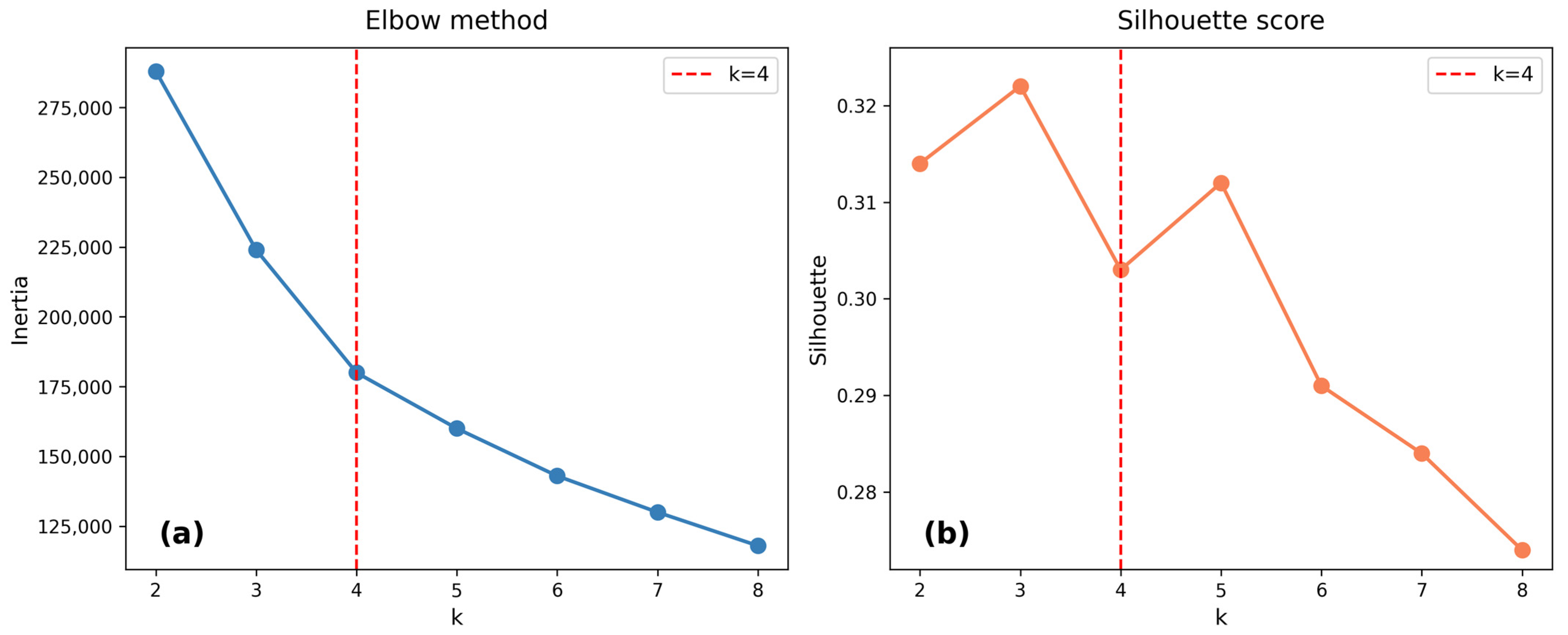
Figure 16.
Community typologies (k = 4, CERI-weighted). Bar chart showing the number and percentage of points in each cluster: Low Risk (20,503; 32.5%), Resilient (14,213; 22.6%), Moderate Risk (20,816; 33.0%), and High Risk (7485; 11.9%).
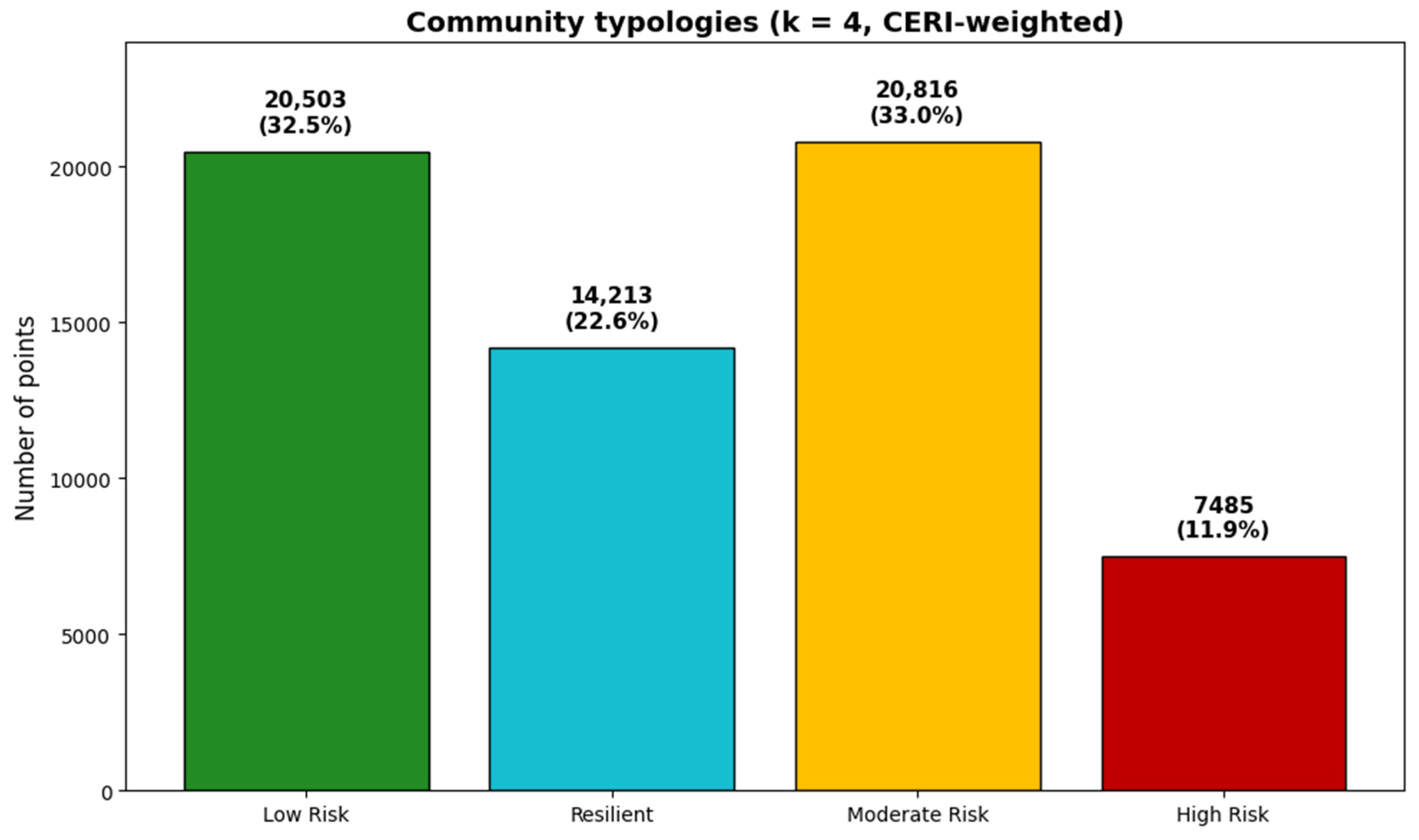
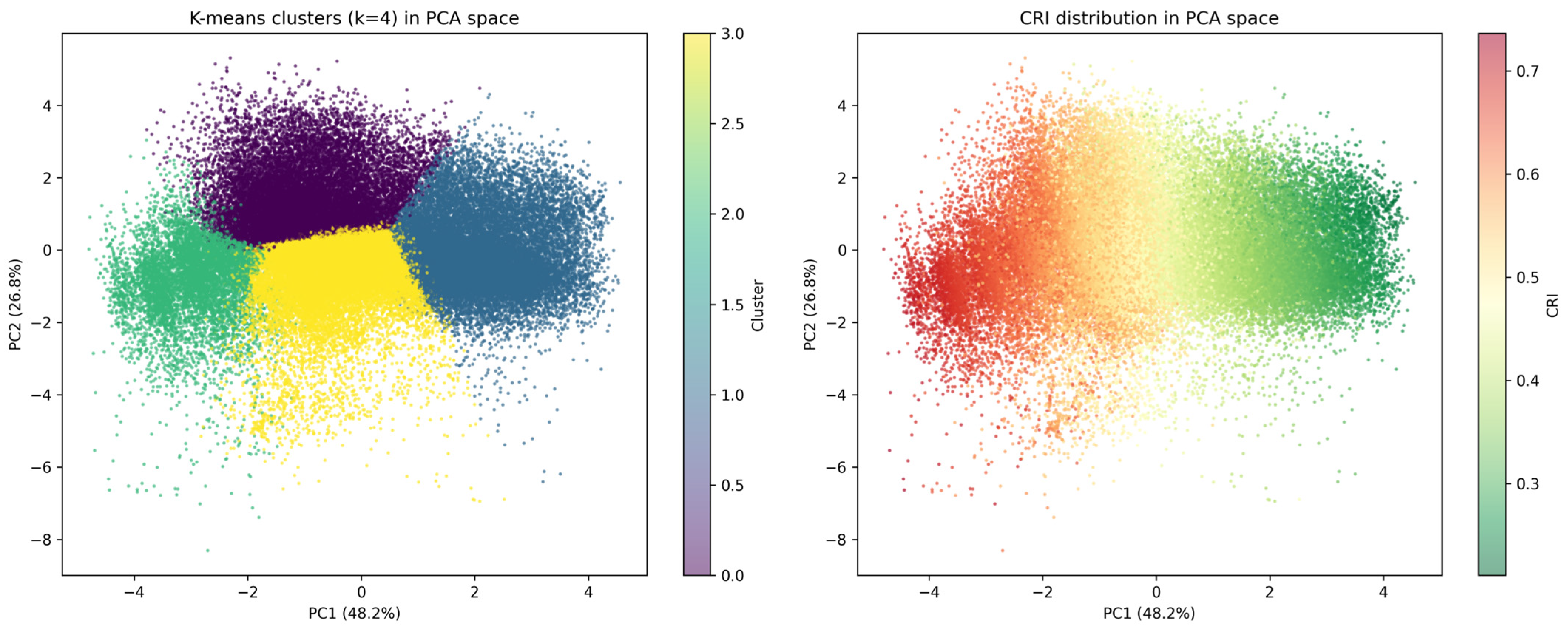
Figure 17.
K-means clusters in PCA space (k = 4) alongside CRI distribution in PCA space. (Left) panel: four distinct clusters with minimal overlap. (Right) panel: CRI values showing that high CRI clusters at negative PC1 values, confirming that the CRI primarily captures the economic vulnerability dimension.
The spatial distribution of these four typologies across the study area is shown in Figure 18. High Risk communities are concentrated along the Chi River corridor in the northern and eastern portions of the study area, while Low Risk communities dominate the southern and central upland areas.
Figure 18.
Spatial distribution of community typologies (k = 4, CERI-weighted). High Risk communities are concentrated along the Chi River corridor in the northern and eastern portions of the study area, while Low Risk communities dominate the southern and central upland areas.
The distinct characteristics of each cluster are further illustrated by the radar chart (Figure 19), which highlights that the High Risk cluster is distinguished by the highest NELI (0.806), highest flood_freq (2.024 events), and lowest CERI (0.484). In contrast, the Resilient cluster is characterized by high CERI (0.708) and moderate NELI (0.614) despite low mean flood frequency (0.097 events).
Figure 19.
Cluster profiles (radar chart) for the four community typologies. The High Risk cluster is distinguished by the highest NELI (0.806), highest flood_freq (2.024 events), and lowest CERI (0.484), while the Resilient cluster is characterized by high CERI (0.708) and moderate NELI (0.614) despite low mean flood frequency (0.097 events). The Low Risk cluster shows the lowest NELI (0.193) and lowest MDRI (0.010).
A direct comparison of the Resilient and Low Risk clusters reveals that the Resilient cluster has substantially higher NELI (median ≈ 0.65 vs. 0.18), higher CERI (median ≈ 0.71 vs. 0.59), and higher NDVI_2024 (median ≈ 0.31 vs. 0.22) than the Low Risk cluster, despite both having zero mean flood frequency. These key differences are visualized using boxplots (Figure 20). This finding indicates that the Resilient group is not simply a low-exposure group but rather a group characterized by high adaptive capacity and ecosystem services that offset moderate economic vulnerability. The distinction between Resilient and Low Risk communities has important policy implications: interventions in Resilient areas should focus on maintaining and strengthening adaptive capacity, while interventions in Low Risk areas should focus on preventing the emergence of vulnerability as development pressures increase.
Figure 20.
Boxplots of indices by cluster. Six panels showing the distribution of (a) NELI, (b) ILSI, (c) ACI, (d) CERI, (e) flood_freq, and (f) CRI across the four community typologies. High Risk shows the highest NELI, ILSI, ACI, and flood_freq, but the lowest CERI, while Resilient shows the highest CERI despite moderate exposure.
To further illustrate these distinctions, the distributions of the four community typologies across all indices and flood frequency are shown in Figure 21. The High Risk cluster shows the highest NELI, ILSI, ACI, and flood_freq, but the lowest CERI, while the Resilient cluster shows the highest CERI despite moderate exposure.
Figure 21.
Resilient vs. Low Risk—key differences. Boxplots comparing flood frequency, NELI, CERI, and NDVI 2024 between the Resilient and Low Risk clusters. The Resilient cluster has substantially higher NELI (median ≈ 0.65 vs. 0.18), higher CERI (median ≈ 0.71 vs. 0.59), and higher NDVI_2024 (median ≈ 0.31 vs. 0.22) than the Low Risk cluster, despite both having zero mean flood frequency.
3.8. Principal Component Analysis of Risk Dimensions
Principal Component Analysis (PCA) was performed on standardized predictor variables to examine the underlying structure of flood risk. The first two principal components explained 75.5% of total variance, with PC1 accounting for 50.6% and PC2 for 24.9% (Figure 22).
Figure 22.
Principal Component Analysis (PCA)—Full Data. (a) Scree plot showing the variance explained by each principal component. PC1 explains 50.6% of total variance, PC2 explains 24.9%, and the first two components collectively explain 75.5% of variance. (b) PCA biplot showing the distribution of points (colored by CRI) and variable loadings. PC1 is strongly associated with vulnerability indices (NELI, ACI, MDRI) and negatively with CERI, representing an “economic vulnerability” dimension. PC2 is associated with flood frequency and topographic variables, representing a “physical exposure” dimension.
PC1 was strongly associated with socioeconomic vulnerability indices (NELI, ACI, MDRI) and negatively with CERI, representing an “economic vulnerability” dimension, while PC2 was associated with flood frequency and elevation (DEM) and represents a “physical exposure” dimension. The orthogonal nature of these components confirms that economic vulnerability and physical exposure are distinct but complementary dimensions of flood risk, and that communities may be vulnerable through different pathways.
4. Discussion
4.1. Physical Exposure Dominates Flood Occurrence, Socioeconomic Vulnerability Modulates Consequences
The clearest empirical result of this study is the separation between the drivers of flood occurrence and the modulators of flood consequences. The spatially blocked Random Forest classifier trained on the independent 2025 flood outcome shows that physical and environmental variables—surface moisture (mndwi_2024), elevation (DEM), and flood frequency (flood_freq)—collectively account for 68.2% of SHAP importance, while socioeconomic indices contribute 31.8% (Figure 12). Out-of-sample testing of the composite indices against the same occurrence outcome gives a concordant picture: NELI achieved the highest AUC (0.910), followed by ACI (0.891), ILSI (0.844), MDRI (0.838), and CERI (0.816 after inversion), while the out-of-sample CRI AUC was 0.771 (Section 3.4). The two lines of evidence therefore agree that physical exposure is the dominant control on whether flooding occurs, while socioeconomic conditions act primarily on the consequences of flooding once it occurs.
The dominance of surface moisture (mndwi_2024) as the single most important predictor (mean |SHAP| = 0.1065) is consistent with the hydrology of the Chi River floodplain. MNDWI captures surface water and saturated soils, which directly control whether a location experiences overbank flooding during the monsoon [60,61,62]. The sharp transition at mndwi_2024 ≈ −0.15 (Figure 14) suggests a critical moisture level above which flood probability rises abruptly, a pattern consistent with a hydrological tipping point in low-relief floodplains [53]. The DEM threshold at approximately 145 m corresponds to the bankfull elevation of the Chi River, below which overbank flooding occurs regularly [18,20]. These thresholds are not statistical artefacts; they reflect the hydrological processes that govern flood occurrence in this setting.
The more modest but still significant contribution of the socioeconomic indices is theoretically meaningful. NELI ranks third overall (mean |SHAP| = 0.107) and CERI fourth (0.088), indicating that economic vulnerability does influence flood outcomes, but through pathways distinct from the physical drivers of occurrence. This is consistent with the vulnerability framework of Adger [9] and Wisner et al. [12], in which vulnerability is a multidimensional construct that cannot be reduced to physical exposure. The low AUC of ACI (0.891) and MDRI (0.838) against Flood_2025 should not be read as evidence that these indices are uninformative; rather, they capture dimensions of adaptive capacity and development risk that operate on consequences rather than on occurrence.
The practical implication is that flood risk management must address both dimensions. Physical infrastructure—levees, drainage, and land-use regulation—addresses the occurrence dimension. Social protection—income diversification, social capital development, and disaster preparedness—addresses the consequence dimension. Conflating the two, as many composite-index studies do, leads to interventions that address one dimension while neglecting the other [7,8]. The separation demonstrated here provides a defensible basis for assigning policy instruments to the dimension they can actually influence.
Confirmation of Established Knowledge and New Contributions
Several findings in this study confirm what is already well established in the flood-risk literature. Greater flood risk at lower elevations, increased risk with repeated flooding, and the protective role of natural vegetation are consistent with prior work in the Chi River Basin [18,20] and in similar floodplain environments [7,8]. The protective effect of community resilience on flood outcomes also aligns with resilience theory in social–ecological systems [30,31,37,38]. These confirmations are important because they show that the revised modelling framework produces results consistent with the existing literature, which supports the credibility of the new findings.
Three findings, however, represent contributions that extend beyond established knowledge. First, the empirical separation between drivers of flood occurrence and modulators of flood consequences is, to our knowledge, the first explicit demonstration in a tropical floodplain context that these two dimensions can be distinguished statistically using a temporally separated outcome. This separation has practical implications: it suggests that physical infrastructure and social protection address different dimensions of risk and should be planned in parallel rather than treated as substitutes. Second, the multidimensional index framework (NELI, ILSI, ACI, CERI) provides a replicable approach that avoids the circularity that has affected many composite-index studies. The independent validation against the 2025 flood event (AUC = 0.771 for CRI, 0.910 for NELI) provides honest external estimates that are not artifacts of index construction. Third, the identification of a Resilient cluster—characterised by high NELI and high CERI despite continued flood exposure—demonstrates that communities can achieve safety through adaptive capacity rather than through locational advantage. This finding has direct implications for differentiated management strategies: interventions in Resilient areas should focus on maintaining adaptive capacity, while interventions in Low Risk areas should focus on preventing the emergence of vulnerability as development pressures increase.
4.2. The Critical Elevation Threshold and Its Implications
A clear elevation threshold at approximately 145 m, with a 40-fold difference in flood frequency between areas below 145 m (73.5%) and above 155 m (1.8%), is evident directly in the DEM and flood inventory and confirms previous findings in the Chi River Basin [18,20].
Identification and uncertainty. The threshold was identified by examining the empirical flood-frequency distribution across elevation bins of 5 m. The break appears consistently across the 140–150 m range, with the sharpest transition at 145 m, indicating that the threshold is robust to sampling variability. The threshold is independent of the SHAP analysis and provides a simple basis for flood risk zoning.
Interpretation. The threshold effect represents a form of translational symmetry breaking in the elevation–flood relationship. Rather than a smooth gradient where flood risk gradually decreases with elevation, the relationship exhibits a sharp discontinuity: below 145 m flood intensity is uniformly high regardless of other factors; above 155 m it is uniformly low. Only within the 145–155 m transitional zone do other factors (land use, drainage, socio-economic conditions) modulate flood risk [18].
Practical implications. First, it provides a clear, legally defensible basis for land use zoning. The proposed three-tier framework (Red < 145 m, Yellow 145–155 m, Green > 155 m) is simple enough for local governments to implement and enforce. Second, it enables targeted investment: rather than spreading resources evenly across the floodplain, interventions can be concentrated in the Red Zone where they will have the greatest impact. Third, it provides a basis for risk communication: residents can easily understand that areas below 145 m face fundamentally different flood risk than areas above 155 m.
Limitations. The threshold should not be applied rigidly without consideration of local conditions. The SHAP analysis revealed that within the transitional zone (145–155 m), other factors—particularly proximity to tributaries and land use—modulate risk. This suggests that the zoning framework should be applied with flexibility, incorporating local knowledge and additional data layers where available [60]. In contrast, the socioeconomic thresholds identified by SHAP (e.g., NELI ≈ 0.8, ILSI ≈ 0.50) are model-internal dependence patterns derived from a classifier in which the same indices also contribute to the target, and should not be presented as validated intervention criteria.
4.3. Community Resilience as a Protective Factor
The finding that higher community resilience (CERI) consistently reduces risk (r = −0.254, p < 0.001) has important implications for flood risk management. CERI captures multiple dimensions of adaptive capacity: social networks, economic diversification, community cohesion, and disaster preparedness. Communities with high CERI are better able to anticipate, absorb, and recover from flood shocks, reducing their overall vulnerability.
The clustering analysis identified a distinct Resilient cluster (Cluster 2, 22.6% of points) characterized by high CERI (0.708) and moderate NELI (0.614) despite low mean flood frequency (0.097 events). These communities demonstrate that adaptive capacity can offset physical exposure, effectively decoupling flood risk from flood hazard. This finding aligns with resilience theory in social–ecological systems [30,31], which emphasizes that outcomes are determined not by exposure alone, but by the interaction of exposure and adaptive capacity.
The mechanisms through which CERI reduces risk are multiple. Strong social networks enable mutual assistance during and after floods, reducing reliance on external aid [41,52]. Economic diversification—combining farming with off-farm income—provides buffers against crop losses [34]. Community cohesion facilitates collective action for flood preparedness, including maintenance of drainage channels, early warning systems, and evacuation planning [51,52]. These mechanisms are mutually reinforcing: communities with strong social networks are better able to diversify livelihoods, which in turn strengthens community cohesion.
A direct comparison of the Resilient and Low Risk clusters (Figure 20) reveals that the Resilient cluster has substantially higher NELI (median ≈ 0.65 vs. 0.18), higher CERI (median ≈ 0.71 vs. 0.59), and higher NDVI_2024 (median ≈ 0.31 vs. 0.22) than the Low Risk cluster, despite both having low mean flood frequency. This finding indicates that the Resilient group is not simply a low-exposure group but rather a group characterized by high adaptive capacity and ecosystem services that offset moderate economic vulnerability. The distinction between Resilient and Low Risk communities has important policy implications: interventions in Resilient areas should focus on maintaining and strengthening adaptive capacity, while interventions in Low Risk areas should focus on preventing the emergence of vulnerability as development pressures increase.
4.4. Land Use Change and Its Implications for Flood Risk
The analysis of land use transitions from 2015 to 2023 reveals several patterns with implications for flood risk. While most areas remained stable (86.1%), urbanization (4.6%) and deforestation (0.6%) represent potentially significant drivers of increased flood risk. Urbanization increases impervious surfaces, reduces infiltration, and accelerates runoff, potentially amplifying flood peaks downstream [13,14]. Deforestation reduces rainfall interception and soil infiltration capacity, increasing surface runoff and erosion [15,16].
The finding that agricultural areas contain the highest proportion of High Risk points (5.9%) while Forest areas show the lowest (1.1%) reinforces the protective role of natural vegetation. Forests provide multiple flood mitigation services: rainfall interception, infiltration enhancement, soil stabilization, and flow regulation [17,18]. The conversion of forest to agriculture (deforestation) therefore represents a double loss: not only does it reduce natural flood protection, but it also increases the area of vulnerable agricultural land.
However, the relationship between land use and flood risk is not straightforward. Agricultural areas are often located in floodplains because of fertile soils and water availability, creating inherent flood exposure. The challenge is to manage agricultural systems in ways that reduce vulnerability while maintaining productivity. This might include: (1) promoting flood-tolerant crop varieties; (2) adopting conservation agriculture practices that maintain soil infiltration capacity; (3) developing drainage systems that reduce waterlogging; and (4) integrating floodwater storage (e.g., farm ponds, check dams) into agricultural landscapes [43].
The conversion of water bodies to agriculture (0.5%) is particularly concerning because it reduces flood storage capacity. Wetlands and floodplains act as natural sponges, absorbing floodwaters and reducing peak flows downstream. Their conversion to agriculture therefore increases flood risk not only locally but also for downstream communities. This finding supports the conservation and restoration of wetlands as a nature-based solution for flood risk reduction [19,20].
4.5. Methodological Contributions: Integrating Machine Learning with Vulnerability Assessment
This study makes several methodological contributions to flood risk assessment.
First, it demonstrates the utility of Random Forest for distinguishing between two conceptually different classification tasks: reproducing a constructed risk typology and predicting an independent flood outcome. The three-class classifier that predicted CRI-derived risk classes achieved per-class accuracy of 96.6–98.3% (Figure 11), which confirms that the composite indices reproduce the intended typology consistently. This result is presented as a consistency check on index construction rather than as independent validation, because the target classes are constructed from the same indices used as predictors. The binary classifier that predicted the independent 2025 flood outcome achieved AUC-ROC = 0.9989 and AUC-PR = 0.7657 (Model B). To test whether the socioeconomic indices add incremental predictive value beyond physical exposure, we compared Model B with a physical-only model (Model D, AUC-PR = 0.7499). The comparison showed that adding the four socioeconomic indices improved AUC-PR modestly (Δ = +0.0158), indicating that socioeconomic indices carry incremental information about flood occurrence beyond physical exposure alone. It is also worth noting that the relatively low AUC-PR values, despite high AUC-ROC values, reflect the strongly imbalanced nature of the flood outcome (positive rate = 1.41%), for which AUC-PR is a more informative metric than AUC-ROC.
Second, the composite indices developed in this study (NELI, ILSI, ACI, CERI) provide a replicable framework for integrated vulnerability assessment, with MDRI reported separately as a contextual indicator of maladaptive development risk. Unlike single-indicator approaches that capture only one dimension of vulnerability, these indices integrate economic, social, and environmental dimensions. The out-of-sample test against the 2025 flood occurrence (Section 3.4) shows that the indices carry genuine predictive information about a temporally separated occurrence outcome, with NELI achieving the highest AUC (0.910), followed by ACI (0.891), ILSI (0.844), and CERI (0.816 after inversion). This validates the indices’ association with flood exposure, not their validity as measures of flood consequences. This suggests they could be adapted for use in other flood-prone regions, with appropriate calibration to local conditions [28].
Third, the integration of SHAP analysis enables interpretation of the model’s predictions and reveals non-linear relationships that would be missed by linear models. Two categories of thresholds must be distinguished. The mndwi_2024 threshold (≈−0.15) and the DEM threshold (≈145 m) are evident directly in the underlying raster data and are consistent with hydrological expectations, so they can be used with confidence in zoning and early warning. In contrast, the socioeconomic thresholds (NELI ≈ 0.8, ILSI ≈ 0.50) are model-internal dependence patterns derived from a classifier in which the same indices also contribute to the target, and should be treated as descriptive rather than prescriptive. This distinction represents a significant advance over “black box” machine learning approaches that provide predictions without explanation [55].
Fourth, the two-stage analytical framework combining unsupervised (K-means clustering) and supervised (Random Forest) learning provides a robust approach to exploratory classification. The clustering results identify distinct community types that require differentiated management strategies (Section 3.7), while the Random Forest results identify the physical and socioeconomic drivers of flood occurrence. This framework could be applied to other hazard types (drought, coastal erosion, heatwaves) and other regions.
However, several methodological limitations should be acknowledged. First, the composite indices are based on available data and may not capture all dimensions of vulnerability. Qualitative factors—such as governance capacity, institutional trust, and cultural attitudes—are not reflected in the indices but may influence resilience. Second, the temporal scope (2017–2025) is relatively short for assessing long-term vulnerability trends. Third, the spatial resolution (point-based sampling) may not capture intra-community heterogeneity. Fourth, the SHAP-derived socioeconomic thresholds are not independent intervention criteria, because they are derived from a classifier in which the same indices contribute to the target. Future research should address these limitations through household surveys, longer time series, and higher-resolution spatial analysis.
4.6. Policy Implications for Sustainable Flood Risk Management
The findings of this study have several implications for policy and practice in flood risk management:
Elevation-based zoning: The identification of a critical elevation threshold at 145 m provides a simple, legally defensible basis for land use regulation. We recommend that local governments adopt a three-tier zoning framework (Red < 145 m, Yellow 145–155 m, Green > 155 m), with progressively more stringent restrictions in higher-risk zones. This framework should be applied flexibly, incorporating local knowledge and additional data layers where available.
Targeted interventions: The concentration of High Risk areas along the Chi River corridor enables spatial targeting of interventions. Rather than spreading resources evenly across the district, investments should be concentrated in the Red Zone where risk is highest. The perfect recall of the Random Forest model (1.000 for High Risk) ensures that no high-risk locations are missed in screening.
Resilience-building: The protective role of community resilience suggests that investments in social capital, livelihood diversification, and disaster preparedness can yield substantial risk reduction benefits. These interventions are relatively low-cost compared to structural measures but require sustained commitment and community engagement.
Land use planning: The association between land use and flood risk suggests that land use planning should be a central component of flood risk management. Forest conservation, sustainable agriculture, and wetland restoration can contribute to flood risk reduction while providing multiple co-benefits (biodiversity conservation, carbon sequestration, livelihood support).
Integrated early warning: The predictive performance of the Random Forest model suggests that composite vulnerability indices could be integrated into early warning systems. By combining flood forecasting (physical exposure) with vulnerability assessment (socio-economic susceptibility), early warning systems could provide more targeted and actionable information.
Maladaptive development: Although MDRI is not included as a predictor in the primary flood-occurrence model (Model B), its earlier conceptualization and the findings from Model C (Section 3.5) suggest that development in flood-prone areas should be carefully regulated, although this contribution should be treated as descriptive rather than as a validated causal effect. Restricting urbanization in high-risk zones and promoting sustainable land use planning remain prudent measures for preventing maladaptive development patterns that increase long-term vulnerability [40,41,51].
4.7. Limitations and Future Research Directions
Several limitations of this study should be acknowledged:
Validation scope. The independent validation tests whether the composite indices predict flood occurrence, not whether they measure flood consequences. Direct validation of consequence-related performance would require household-level data on economic loss, recovery time, and displacement, which were unavailable in this study.
Temporal scope: The study covers the period 2017–2025, which is relatively short for assessing long-term vulnerability trends and the effects of climate change. Future research should extend the temporal scope to multiple decades, incorporating climate projections to assess evolving risk under different emissions scenarios [21].
Spatial resolution: The point-based sampling framework (63,017 points) provides good spatial coverage but may not capture intra-community heterogeneity. Higher-resolution analysis at the household or parcel level would provide more detailed insights into vulnerability patterns.
Data availability: The composite indices rely on available data and may not capture all dimensions of vulnerability. Qualitative factors—such as governance capacity, institutional trust, and cultural attitudes—are not reflected in the indices but may influence resilience. Future research should integrate household surveys and qualitative methods to capture these dimensions.
Causality: The analysis is correlational rather than causal. While we have identified strong associations between vulnerability indices and flood risk, we cannot definitively establish causality. Future research should employ quasi-experimental methods (difference-in-differences, instrumental variables) to estimate causal effects.
Generalizability: The findings are specific to the Chi River floodplain and may not be directly transferable to other regions with different hydrological, climatic, or socioeconomic conditions. Replication studies in other flood-prone regions (e.g., Mekong Delta, Chao Phraya Basin, other floodplains) would establish generalizability.
Model uncertainty: While the Random Forest model achieves strong discrimination under spatial block cross-validation (AUC-ROC = 0.9989, AUC-PR = 0.7657 for Model B), there is some uncertainty in predictions, particularly for Moderate Risk areas where misclassification rates are slightly higher. Future research should quantify prediction uncertainty and incorporate it into decision-making.
Climate change: The study is retrospective rather than prospective. Climate change is projected to increase flood frequency and intensity in Southeast Asia [21], potentially altering the relationships identified in this study. Future research should incorporate climate projections to assess how flood risk may evolve under different emissions scenarios.
4.8. Contributions to Sustainable Development Goals
This study contributes directly to several Sustainable Development Goals (SDGs):
SDG 11 (Sustainable Cities and Communities): The elevation-based zoning framework and spatial targeting of interventions support the development of resilient communities (SDG 11.5). The identification of High Risk areas enables targeted disaster risk reduction, reducing flood-related deaths and economic losses.
SDG 13 (Climate Action): The integrated vulnerability assessment and early warning framework support climate change adaptation and resilience building (SDG 13.1). The emphasis on community resilience and adaptive capacity aligns with the Paris Agreement’s focus on building adaptive capacity.
SDG 15 (Life on Land): The protective role of forests and the risks of deforestation support the conservation and sustainable use of terrestrial ecosystems (SDG 15.1). The findings support land degradation neutrality and the restoration of degraded land (SDG 15.3).
SDG 2 (Zero Hunger): The vulnerability of agricultural areas to flood risk has implications for food security (SDG 2.4). The identification of High Risk agricultural areas enables targeted support for sustainable agriculture and climate adaptation.
SDG 6 (Clean Water and Sanitation): The risks associated with water body conversion highlight the importance of protecting water-related ecosystems (SDG 6.6). The wetland restoration recommendation supports water quality and flood regulation.
5. Conclusions
This study developed and applied a multi-dimensional flood risk assessment framework for Mueang Maha Sarakham District, integrating six composite indices (NELI, ILSI, ACI, CERI, MDRI, CRI) across 63,017 spatial points using Random Forest, SHAP analysis, PCA, and K-means clustering.
The analysis revealed a fundamental distinction between the drivers of flood occurrence and the modulators of flood consequences. Physical and environmental variables—surface moisture (mndwi_2024), elevation (DEM), and flood frequency—collectively account for 68.2% of SHAP importance in predicting the 2025 flood event, while socioeconomic indices contribute 31.8%. A physical-only Random Forest model achieved AUC-PR = 0.7499, compared with AUC-PR = 0.7657 when the four socioeconomic indices were added, indicating that socioeconomic indices carry modest incremental information about flood occurrence beyond physical exposure, while their primary role is in modulating flood consequences. A critical elevation threshold of approximately 145 m was identified, with a 40-fold difference in flood frequency between areas below 145 m (73.5%) and above 155 m (1.8%). The spatially blocked Random Forest model achieved AUC-ROC = 0.9989 and AUC-PR = 0.7657 for predicting the 2025 flood outcome, and out-of-sample testing against the temporally separated 2025 flood occurrence confirmed that the composite indices carry information about flood exposure (NELI AUC = 0.910, ACI AUC = 0.891, ILSI AUC = 0.844, CERI AUC = 0.816 after inversion, CRI AUC = 0.771); this does not validate them as measures of flood consequences.
Four distinct community types were identified: Low Risk (32.5%), Resilient (22.6%), Moderate Risk (33.0%), and High Risk (11.9%). The Resilient cluster, characterized by high community resilience (CERI = 0.708), demonstrates that adaptive capacity can effectively mitigate flood risk even with moderate flood exposure. The distinction between Resilient and Low Risk communities—with Resilient showing higher NELI, CERI, and NDVI despite similar flood exposure—provides a nuanced understanding of how communities can achieve safety through different pathways.
Policy recommendations include: (1) implementing elevation-based zoning (Red < 145 m, Yellow 145–155 m, Green > 155 m); (2) targeting High Risk areas for urgent intervention; (3) strengthening community resilience through social capital development and livelihood diversification; (4) prioritizing forest conservation and wetland restoration; and (5) integrating socio-economic indicators into early warning systems. These findings contribute to SDGs 11, 13, and 15 by providing evidence-based tools for sustainable flood risk management in the Chi River Basin and similar floodplain environments.
Future research should extend the temporal scope to assess long-term vulnerability trends, integrate household surveys to capture qualitative dimensions of vulnerability, and apply the framework to other flood-prone regions to establish generalizability. Future work should prioritise household-level validation of the consequence-related performance of these indices.
Author Contributions
Conceptualization, P.L., B.P. and D.S.; methodology, P.L.; software, P.L.; validation, P.L. and B.P.; formal analysis, P.L.; investigation, P.L. and J.M.; resources, P.L.; data curation, P.L.; writing—original draft preparation, P.L.; writing—review and editing, P.L. and D.S.; visualization, P.L.; supervision, P.L.; project administration, P.L.; funding acquisition, P.L. All authors have read and agreed to the published version of the manuscript.
Funding
This research project was financially supported by Mahasarakham University 16-2570.
Institutional Review Board Statement
Not applicable.
Informed Consent Statement
Not applicable.
Data Availability Statement
The data presented in this study are openly available in Zenodo at https://doi.org/10.5281/zenodo.22178574, reference number [63]. The repository includes the complete dataset in Microsoft Excel format and the full Python code (Python version 3.11; Google Colab, Google LLC, Mountain View, CA, USA) used for all analyses, ma-chine learning model implementation, and figure generation.
Acknowledgments
The authors would like to thank the anonymous reviewers for their valuable comments and suggestions that helped improve this manuscript.
Conflicts of Interest
The authors declare no conflicts of interest.
Appendix A. Provenance of Socioeconomic Proxies
This appendix documents the derivation of the eight socioeconomic proxies used to construct the composite indices (NELI, ILSI, ACI, CERI, MDRI). Because household-level data (occupation, income, housing quality, social capital, and recovery capacity) were not available at the point level, each proxy was derived from land use, spectral indices, and topographic variables. The detailed derivation, weighting scheme, and rationale for each proxy are provided in Section 2.2.5. Table A1 summarizes the provenance.
Table A1.
Provenance of socioeconomic proxies.
Spatial assignment. Each proxy was assigned to the 63,017 points by intersecting the point layer with the corresponding raster (land use, NDVI, VCI, TWI, DEM, proximity to streams) using the rasterio Python library. All intermediate rasters and the assignment script are archived in the Zenodo repository [63].
Limitations. Because household-level data were unavailable, these proxies are indirect measures of socioeconomic conditions and may not fully capture household-level heterogeneity. This limitation is discussed in Section 4.7.
References
- IPCC. Climate Change 2022: Impacts, Adaptation and Vulnerability; Cambridge University Press: Cambridge, UK, 2022. [Google Scholar]
- WMO. State of the Global Climate 2023; WMO-No. 1347; World Meteorological Organization: Geneva, Switzerland, 2024. [Google Scholar]
- Kundzewicz, Z.W.; Kanae, S.; Seneviratne, S.I.; Handmer, J.; Nicholls, N.; Peduzzi, P.; Mechler, R.; Bouwer, L.M.; Arnell, N.; Mach, K.; et al. Flood risk and climate change: Global and regional perspectives. Hydrol. Sci. J. 2014, 59, 1–28. [Google Scholar] [CrossRef] [Scilit]
- MRC. State of the Basin Report 2021; Mekong River Commission: Vientiane, Laos, 2021. [Google Scholar]
- Lebel, L.; Sinh, B.T.; Nikitina, E. Floods in the Mekong Delta: A review of impacts and adaptation. Reg. Environ. Change 2019, 19, 1773–1786. [Google Scholar]
- Thaitakoo, D.; Suthiphisal, P.; Tantayanon, S. Flood vulnerability and adaptation in Northeast Thailand. J. Flood Risk Manag. 2021, 14, e12732. [Google Scholar]
- World Bank. Thai Flood 2011: Rapid Assessment for Resilient Recovery and Reconstruction Planning; The World Bank: Bangkok, Thailand, 2012. [Google Scholar]
- Komori, D.; Nakamura, S.; Kiguchi, M.; Nishijima, A.; Yamazaki, D.; Suzuki, S.; Kawasaki, A.; Oki, K.; Oki, T. Characteristics of the 2011 Chao Phraya River flood in Central Thailand. Hydrol. Res. Lett. 2012, 6, 57–62. [Google Scholar] [CrossRef] [Scilit]
- Smith, K. Environmental Hazards: Assessing Risk and Reducing Disaster; Routledge: London, UK, 2013. [Google Scholar]
- Merz, B.; Kreibich, H.; Schwarze, R.; Thieken, A. Review article “Assessment of economic flood damage”. Nat. Hazards Earth Syst. Sci. 2010, 10, 1697–1724. [Google Scholar] [CrossRef] [Scilit]
- Jongman, B.; Winsemius, H.C.; Aerts, J.C.J.H.; Coughlan de Perez, E.; van Aalst, M.K.; Kron, W.; Ward, P.J. Declining vulnerability to river floods and the global benefits of adaptation. Proc. Natl. Acad. Sci. USA 2015, 112, E2271–E2280. [Google Scholar] [CrossRef] [Scilit] [PubMed]
- Adger, W.N. Vulnerability. Glob. Environ. Change 2006, 16, 268–281. [Google Scholar] [CrossRef] [Scilit]
- Birkmann, J. Measuring Vulnerability to Natural Hazards: Towards Disaster Resilient Societies; United Nations University Press: Tokyo, Japan, 2006. [Google Scholar]
- Brouwer, R.; Akter, S.; Brander, L.; Haque, E. Socioeconomic vulnerability and adaptation to environmental risk: A case study of climate change and flooding in Bangladesh. Risk Anal. 2007, 27, 313–326. [Google Scholar] [CrossRef] [Scilit] [PubMed]
- Wisner, B.; Blaikie, P.; Cannon, T.; Davis, I. At Risk: Natural Hazards, People’s Vulnerability and Disasters, 2nd ed.; Routledge: London, UK, 2004. [Google Scholar]
- Turner, B.L.; Kasperson, R.E.; Matson, P.A.; McCarthy, J.J.; Corell, R.W.; Christensen, L.; Eckley, N.; Kasperson, J.X.; Luers, A.; Martello, M.L.; et al. A framework for vulnerability analysis in sustainability science. Proc. Natl. Acad. Sci. USA 2003, 100, 8074–8079. [Google Scholar] [CrossRef] [Scilit] [PubMed]
- Cutter, S.L.; Boruff, B.J.; Shirley, W.L. Social vulnerability to environmental hazards. Soc. Sci. Q. 2003, 84, 242–261. [Google Scholar] [CrossRef] [Scilit]
- Fekete, A. Validation of a social vulnerability index in context to river-floods in Germany. Nat. Hazards Earth Syst. Sci. 2009, 9, 393–403. [Google Scholar] [CrossRef] [Scilit]
- Tucker, C.J. Red and photographic infrared linear combinations for monitoring vegetation. Remote Sens. Environ. 1979, 8, 127–150. [Google Scholar] [CrossRef] [Scilit]
- Xu, H. Modification of normalised difference water index (NDWI) to enhance open water features in remotely sensed imagery. Int. J. Remote Sens. 2006, 27, 3025–3033. [Google Scholar] [CrossRef] [Scilit]
- Breiman, L. Random forests. Mach. Learn. 2001, 45, 5–32. [Google Scholar] [CrossRef] [Scilit]
- Chen, T.; Guestrin, C. XGBoost: A scalable tree boosting system. In Proceedings of the 22nd ACM SIGKDD International Conference on Knowledge Discovery and Data Mining, San Francisco, CA, USA, 13–17 August 2016; pp. 785–794. [Google Scholar]
- Reichstein, M.; Camps-Valls, G.; Stevens, B.; Jung, M.; Denzler, J.; Carvalhais, N.; Prabhat. Deep learning and process understanding for data-driven Earth system science. Nature 2019, 566, 195–204. [Google Scholar] [CrossRef] [Scilit] [PubMed]
- Buasri, N.; Little, P.; Pumhirunroj, B.; Slack, D. Spatial Asymmetry in Topographic Controls on Flood Intensity: A Machine Learning Investigation of the Chi River Floodplain, Thailand. Symmetry 2026, 18, 1231. [Google Scholar] [CrossRef] [Scilit]
- Prasertsri, N.; Little, P.; Pumhirunroj, B.; Slack, D. Spatio-Temporal Machine Learning for Flood Risk Assessment Under SSP Scenarios: A Case Study of Maha Sarakham, Thailand. Sustainability 2026, 18, 7550. [Google Scholar] [CrossRef] [Scilit]
- Buasri, N.; Littidej, P.; Pumhirunroj, B.; Juanchaiyaphum, J.; Slack, D. Integrated Hydro-Hazard Index (HHI) for Drought-Flood Risk Assessment: A Multi-Temporal Machine Learning Approach. Sustainability 2026, 18, 7448. [Google Scholar] [CrossRef] [Scilit]
- Smit, B.; Wandel, J. Adaptation, adaptive capacity and vulnerability. Glob. Environ. Change 2006, 16, 282–292. [Google Scholar] [CrossRef] [Scilit]
- Hosmer, D.W.; Lemeshow, S.; Sturdivant, R.X. Applied Logistic Regression, 3rd ed.; John Wiley & Sons: Hoboken, NJ, USA, 2013. [Google Scholar]
- Cutter, S.L.; Barnes, L.; Berry, M.; Burton, C.; Evans, E.; Tate, E. A place-based model for understanding community resilience to natural disasters. Glob. Environ. Change 2008, 18, 598–606. [Google Scholar] [CrossRef] [Scilit]
- Tate, E. Social vulnerability indices: A comparative assessment using uncertainty and sensitivity analysis. Nat. Hazards 2012, 63, 325–347. [Google Scholar] [CrossRef] [Scilit]
- Few, R. Flooding, vulnerability and coping strategies: Local responses to a global threat. Prog. Dev. Stud. 2003, 3, 43–58. [Google Scholar] [CrossRef] [Scilit]
- Pelling, M. Adaptation to Climate Change: From Resilience to Transformation; Routledge: London, UK, 2011. [Google Scholar]
- Holling, C.S. Resilience and stability of ecological systems. Annu. Rev. Ecol. Syst. 1973, 4, 1–23. [Google Scholar] [CrossRef] [Scilit]
- Littidej, P.; Kamphulling, P.; Pumhirunroj, B.; Slack, D. Economic Damage Assessment of Flood-affected Areas in Mahasarakham Province of Thailand. Sustainability 2025, 17, 12345. [Google Scholar]
- Béné, C.; Newsham, A.; Davies, M.; Ulrichs, M.; Godfrey-Wood, R. Resilience, poverty and development. J. Int. Dev. 2014, 26, 598–623. [Google Scholar] [CrossRef] [Scilit]
- Magnan, A.K.; Schipper, E.L.F.; Burkett, M.; Bharwani, S.; Burton, I.; Eriksen, S.; Gemenne, F.; Schaar, J.; Ziervogel, G. Addressing the risk of maladaptation to climate change. Wiley Interdiscip. Rev. Clim. Change 2016, 7, 646–665. [Google Scholar] [CrossRef] [Scilit]
- Carter, M.R.; Barrett, C.B. The economics of poverty traps and persistent poverty: An asset-based approach. J. Dev. Stud. 2006, 42, 178–199. [Google Scholar] [CrossRef] [Scilit]
- Ellis, F. Household strategies and rural livelihood diversification. J. Dev. Stud. 1998, 35, 1–38. [Google Scholar] [CrossRef] [Scilit]
- Dercon, S. Income risk, coping strategies, and safety nets. World Bank Res. Obs. 2002, 17, 141–166. [Google Scholar] [CrossRef] [Scilit]
- Dow, K.; Berkhout, F.; Preston, B.L.; Klein, R.J.T.; Midgley, G.; Shaw, M.R. Limits to adaptation. Nat. Clim. Change 2013, 3, 305–307. [Google Scholar] [CrossRef] [Scilit]
- Aldrich, D.P.; Meyer, M.A. Social capital and community resilience. Am. Behav. Sci. 2015, 59, 254–269. [Google Scholar] [CrossRef] [Scilit]
- Drusch, M.; Del Bello, U.; Carlier, S.; Colin, O.; Fernandez, V.; Gascon, F.; Hoersch, B.; Isola, C.; Laberinti, P.; Marti-mort, P.; et al. Sentinel-2: ESA’s optical high-resolution mission for GMES operational services. Remote Sens. Environ. 2012, 120, 25–36. [Google Scholar] [CrossRef] [Scilit]
- Suwanlee, S.R.; Keawsomsee, S.; Pengjunsang, M.; Homtong, N.; Prakobya, A.; Borgogno-Mondino, E.; Sarvia, F.; Somard, J. Monitoring Agricultural Land and Land Cover Change from 2001–2021 of the Chi River Basin, Thailand Using Multi-Temporal Landsat Data Based on Google Earth Engine. Remote Sens. 2023, 15, 4339. [Google Scholar] [CrossRef] [Scilit]
- Kienberger, S.; Blaschke, T.; Zaidi, R.Z. A framework for spatio-temporal scales and concepts in vulnerability assessment. Nat. Hazards 2013, 68, 1323–1341. [Google Scholar] [CrossRef] [Scilit]
- Wang, X.; Xie, H.; Guan, H.; Zhou, X. Different responses of MODIS-derived NDVI to root-zone soil moisture in semi-arid and humid regions. J. Hydrol. 2007, 340, 12–24. [Google Scholar] [CrossRef] [Scilit]
- Zhang, L.; Jiao, W.; Zhang, H.; Huang, C.; Tong, Q. Studying drought phenomena in the Continental United States in 2011 and 2012 using various drought indices. Remote Sens. Environ. 2017, 190, 96–106. [Google Scholar] [CrossRef] [Scilit]
- Gao, B.C. NDWI—A normalized difference water index for remote sensing of vegetation liquid water from space. Remote Sens. Environ. 1996, 58, 257–266. [Google Scholar] [CrossRef] [Scilit]
- Kogan, F.N. Application of vegetation index and brightness temperature for drought detection. Adv. Space Res. 1995, 15, 91–100. [Google Scholar] [CrossRef] [Scilit]
- Moore, I.D.; Grayson, R.B.; Ladson, A.R. Digital terrain modelling: A review of hydrological, geomorphological, and biological applications. Hydrol. Process. 1991, 5, 3–30. [Google Scholar] [CrossRef] [Scilit]
- Beven, K.J.; Kirkby, M.J. A physically based, variable contributing area model of basin hydrology. Hydrol. Sci. Bull. 1979, 24, 43–69. [Google Scholar] [CrossRef] [Scilit]
- Putnam, R.D. Bowling Alone: The Collapse and Revival of American Community; Simon and Schuster: New York, NY, USA, 2000. [Google Scholar]
- Pfefferbaum, B.; Pfefferbaum, R.L.; Van Horn, R.L. Community resilience interventions: Participatory, assessment-based, action-oriented processes. Am. Behav. Sci. 2015, 59, 238–253. [Google Scholar]
- Barnett, J.; O’Neill, S. Maladaptation. Glob. Environ. Change 2010, 20, 211–213. [Google Scholar] [CrossRef] [Scilit]
- Fisher, R.A. Statistical Methods for Research Workers, 14th ed.; Oliver and Boyd: Edinburgh, UK, 1970. [Google Scholar]
- Lundberg, S.M.; Lee, S.I. A unified approach to interpreting model predictions. In Advances in Neural Information Processing Systems 30; Curran Associates: Red Hook, NY, USA, 2017; pp. 4765–4774. [Google Scholar]
- Jolliffe, I.T. Principal Component Analysis, 2nd ed.; Springer: New York, NY, USA, 2002. [Google Scholar]
- MacQueen, J. Some methods for classification and analysis of multivariate observations. In Proceedings of the Fifth Berkeley Symposium on Mathematical Statistics and Probability; University of California Press: Berkeley, CA, USA, 1967; pp. 281–297. [Google Scholar]
- Moran, P.A.P. Notes on continuous stochastic phenomena. Biometrika 1950, 37, 17–23. [Google Scholar] [CrossRef] [Scilit]
- Pearson, K. Notes on regression and inheritance in the case of two parents. Proc. R. Soc. Lond. 1895, 58, 240–242. [Google Scholar] [CrossRef] [Scilit]
- Suwanwerakamtorn, R. Floodplain drought paradox: Hydrological analysis of the Chi River Basin. Hydrol. Sci. J. 2022, 67, 1234–1248. [Google Scholar]
- Phakdi, K.; Srisuk, K. Hydrogeology of the Khorat Plateau: Groundwater resources and drought vulnerability. J. Groundw. Sci. Eng. 2019, 7, 156–168. [Google Scholar]
- Bates, P.D.; Trigg, M.A.; Neal, J.C.; Dabrowski, A. Hydrodynamic modelling of river flood inundation. Water Resour. Res. 2013, 49, 5270–5285. [Google Scholar]
- Littidej, P. Python Code for Novel Composite Indices for Flood Risk Assessment Integrating Socio-Economic Vulnerability, Physical Exposure, and Community Resilience in the Chi River Basin, Thailand; Zenodo: Geneva, Switzerland, 2026. [Google Scholar] [CrossRef]
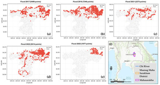
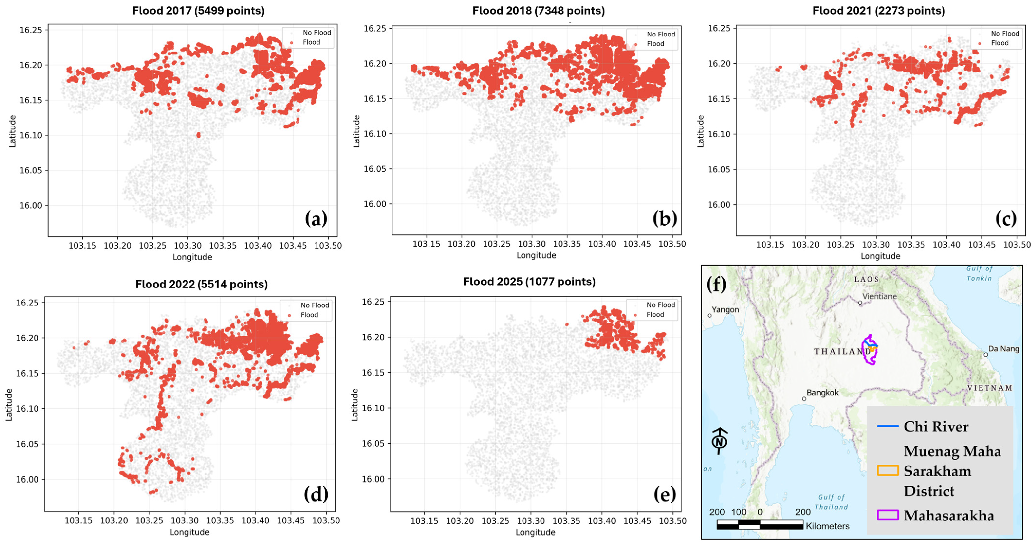
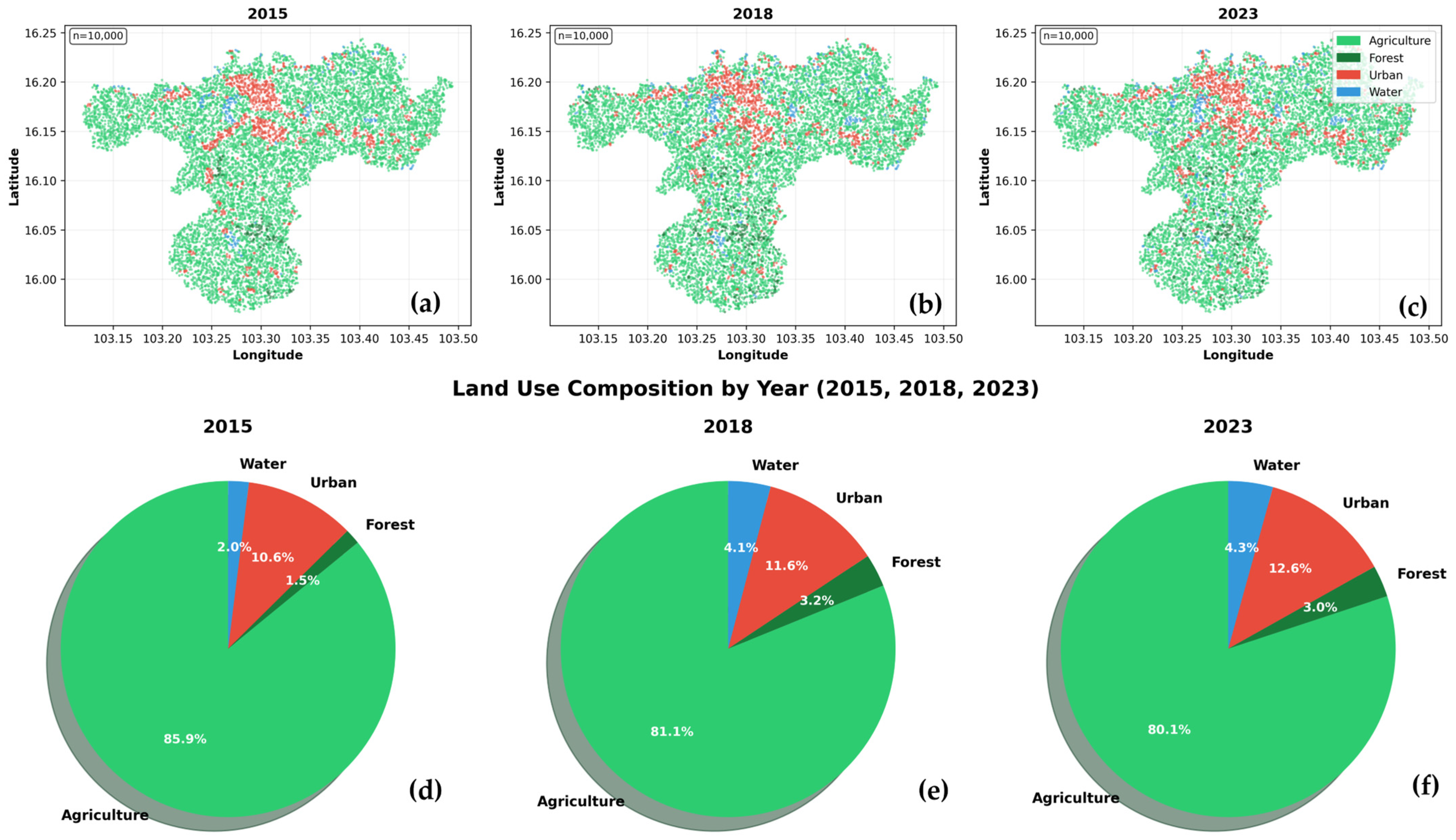
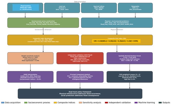
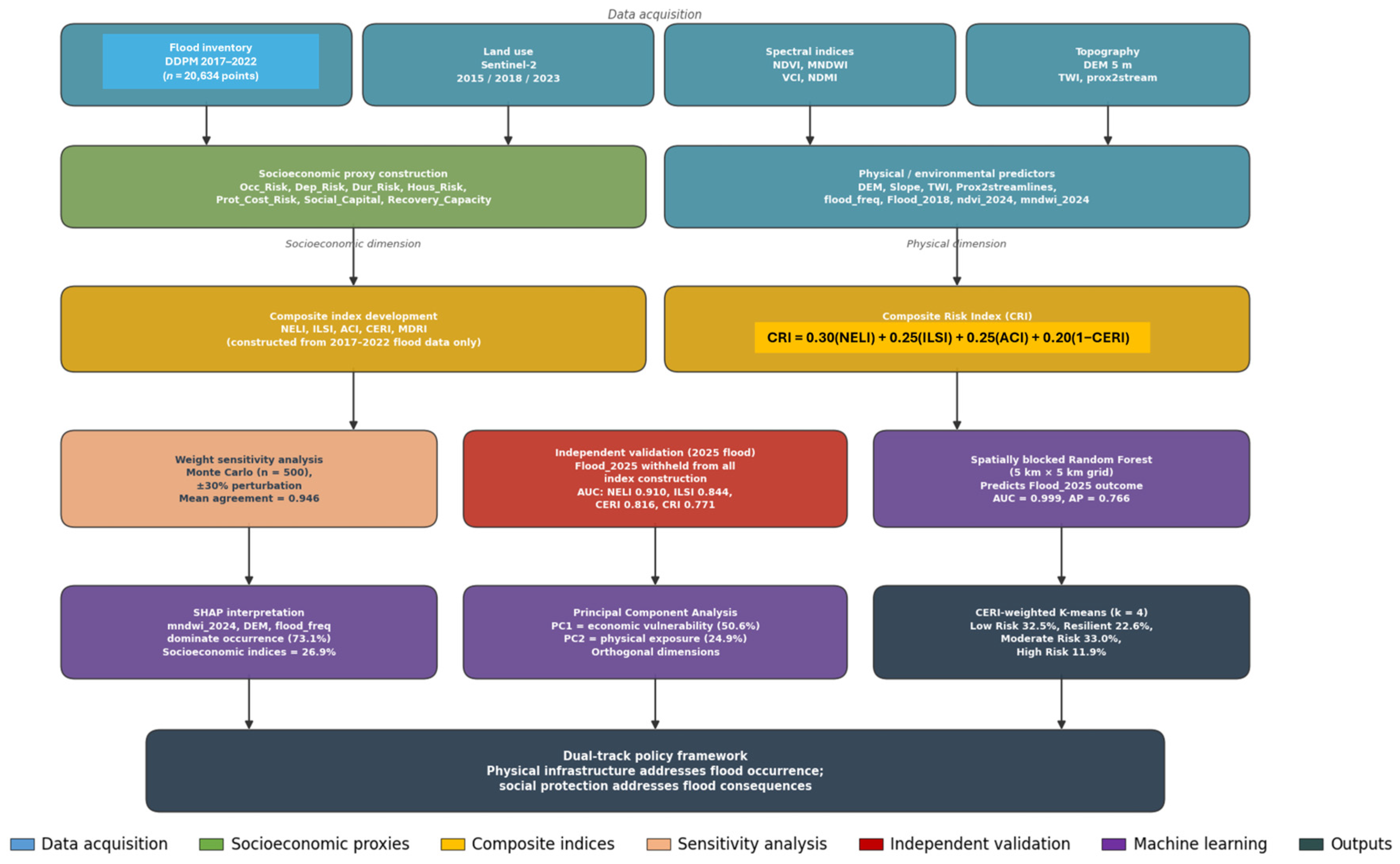
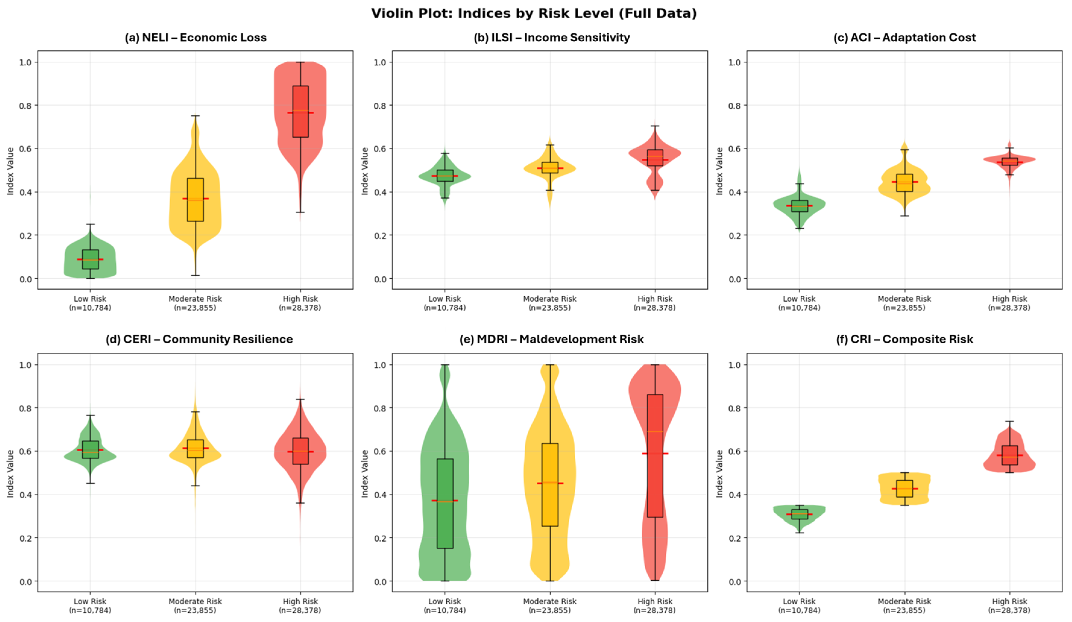
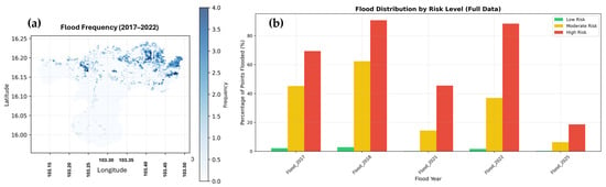
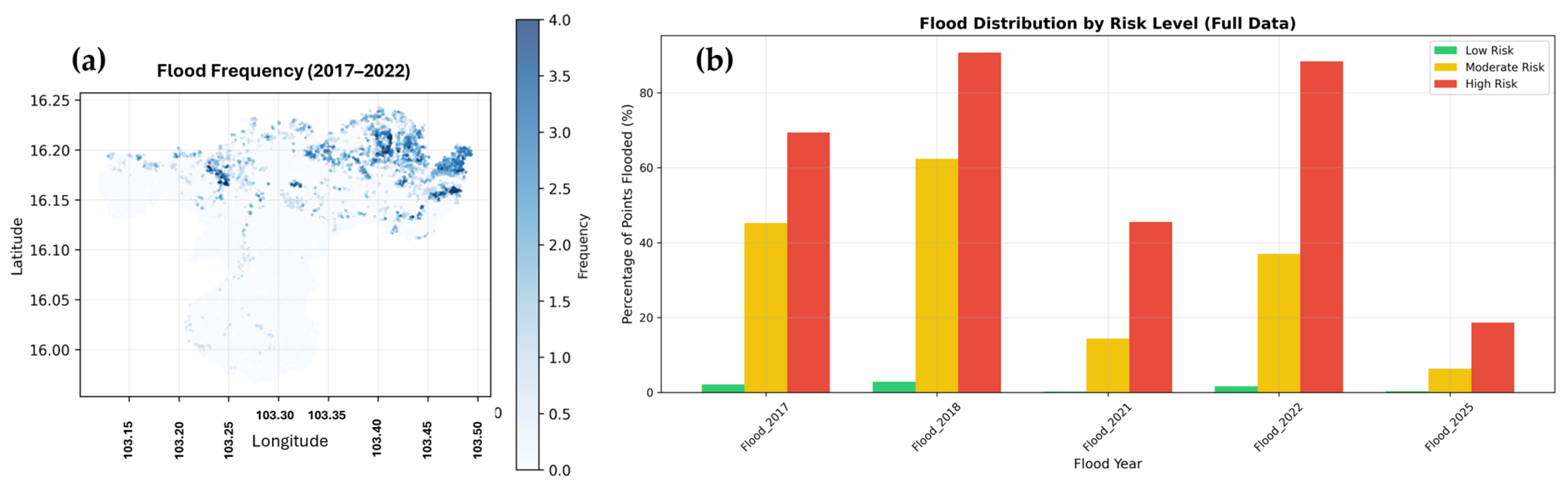
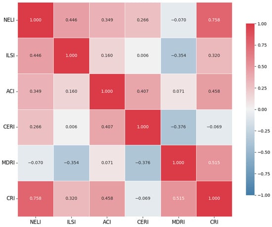
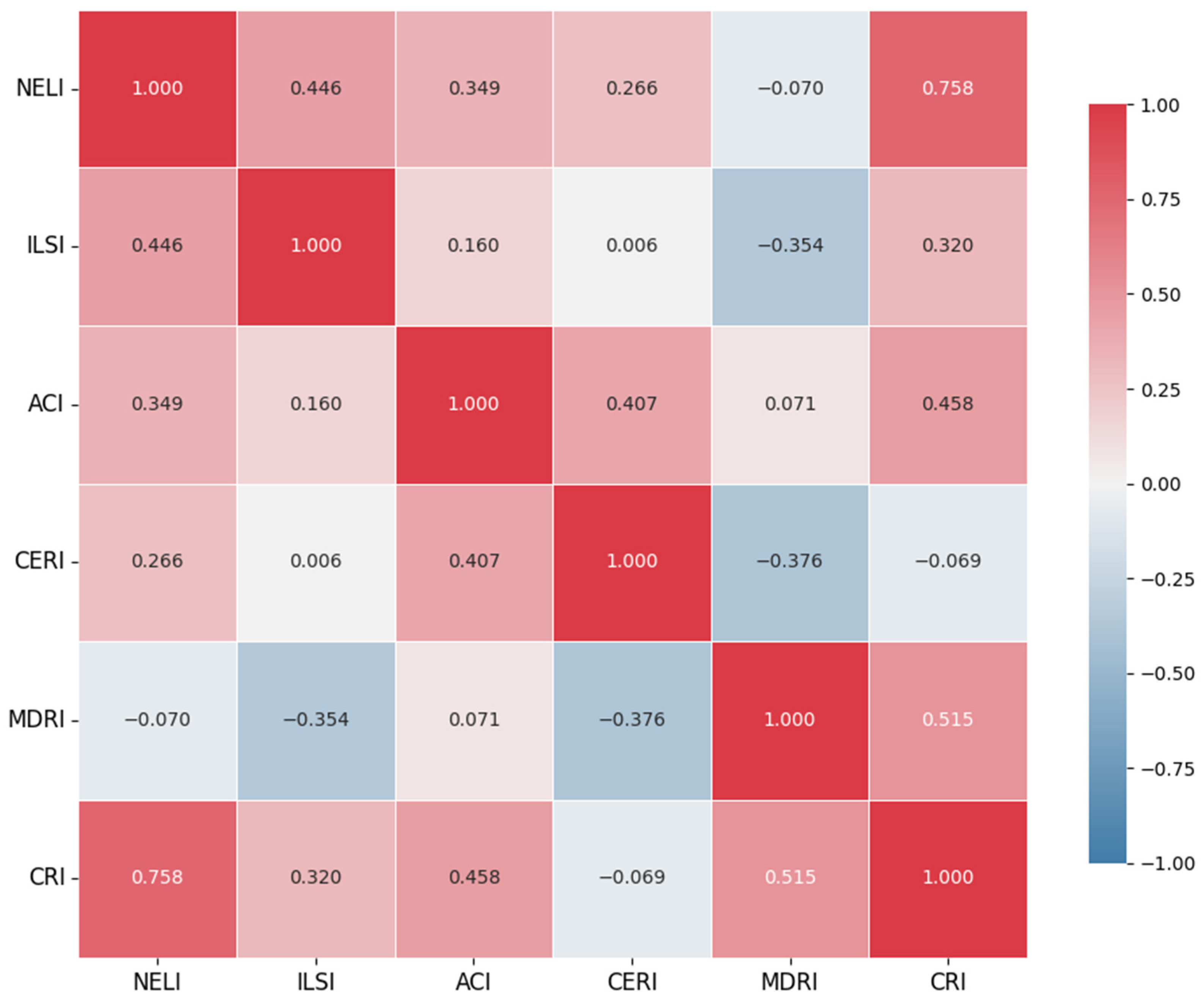
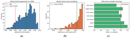
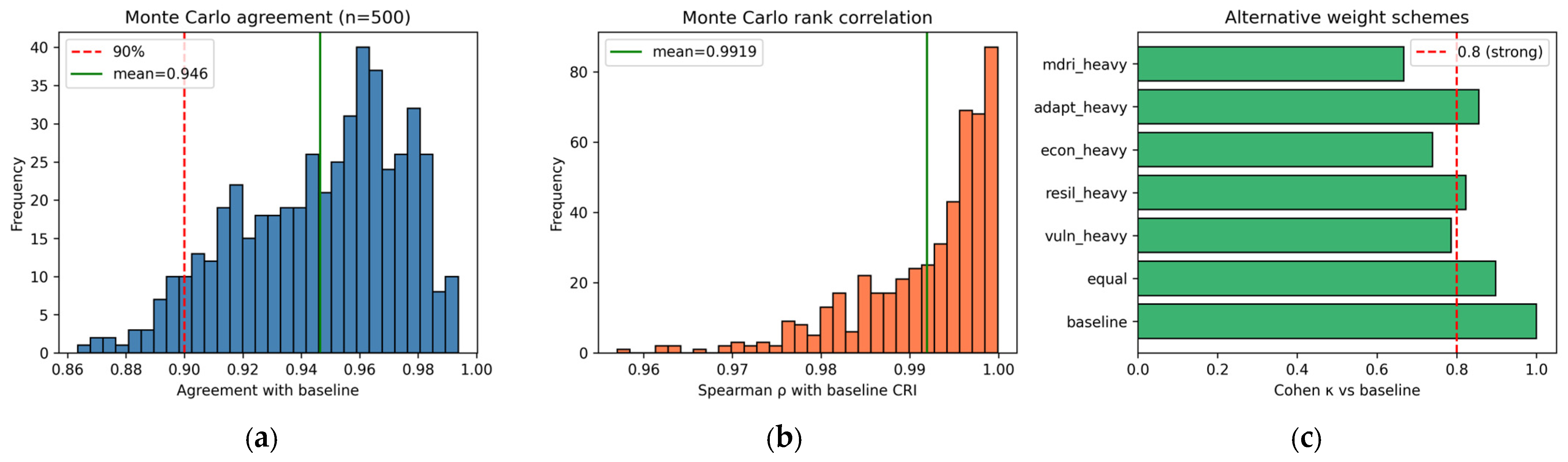
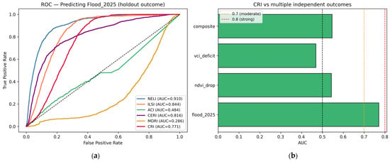
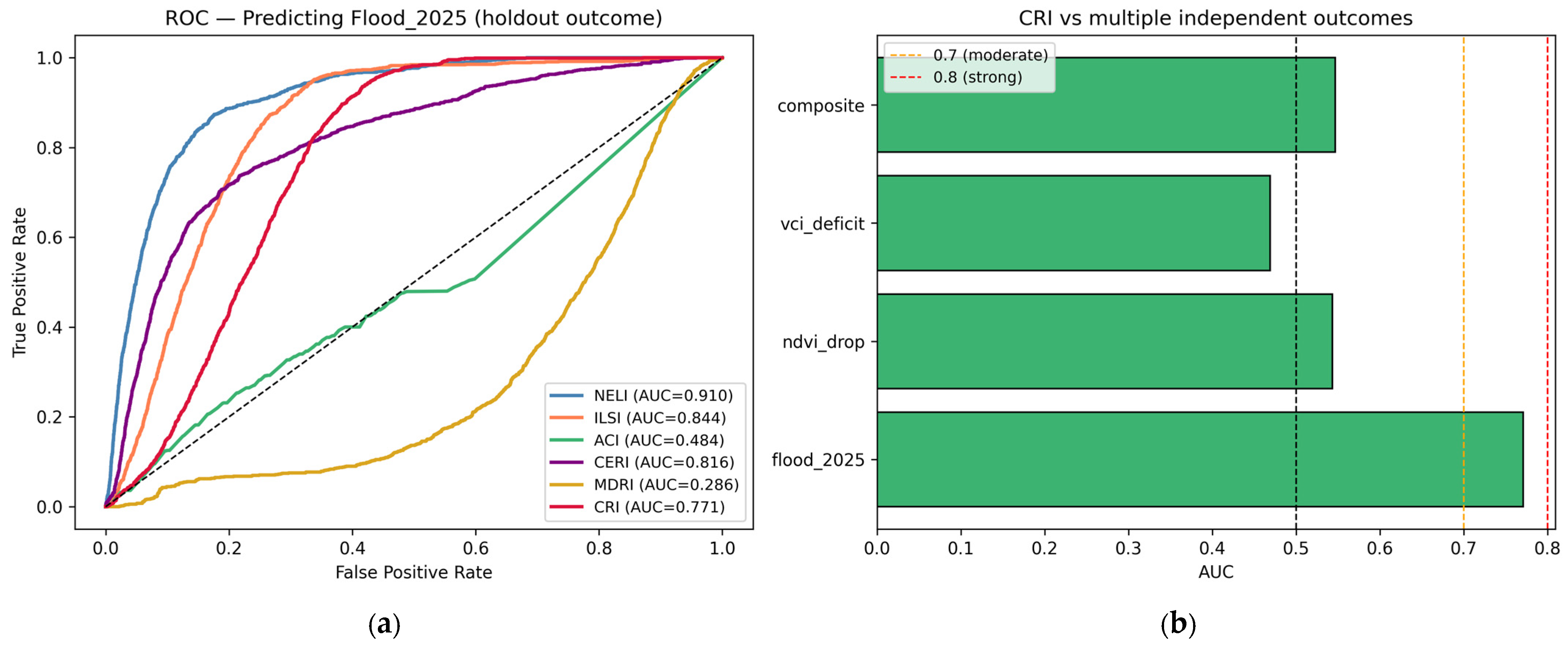
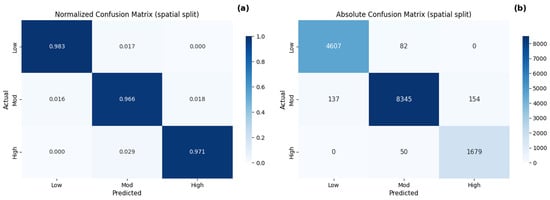
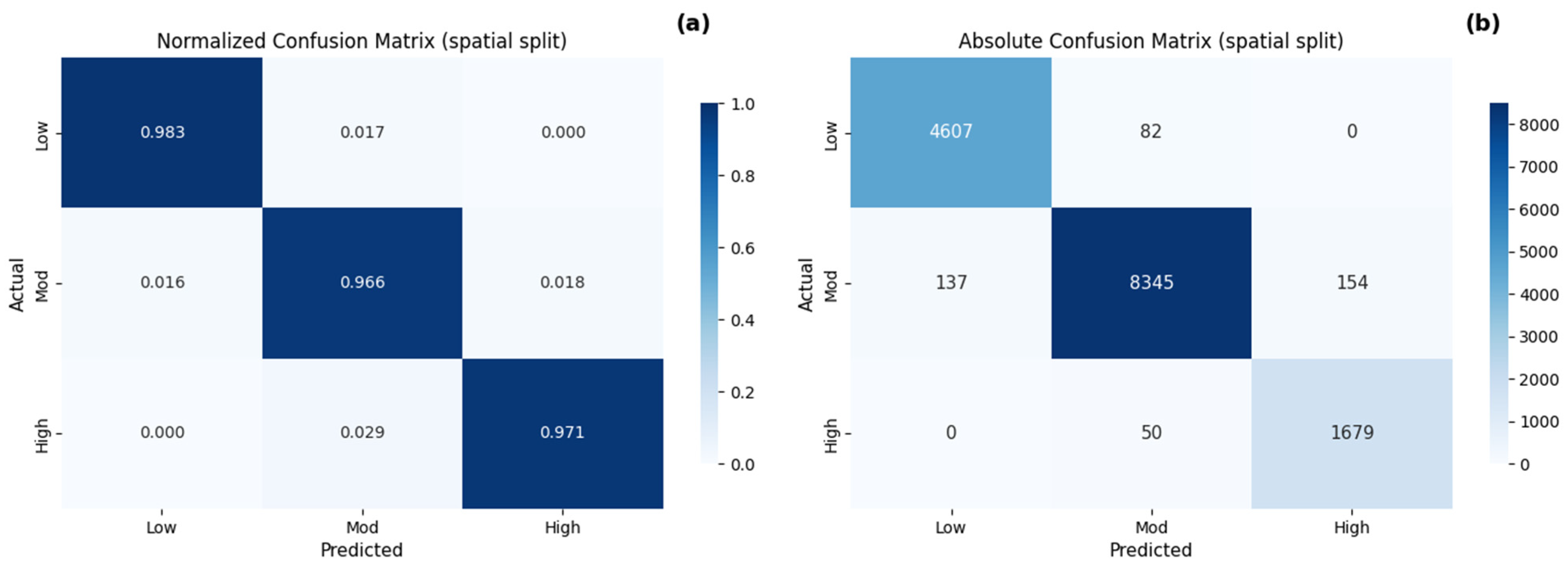
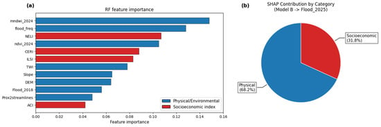
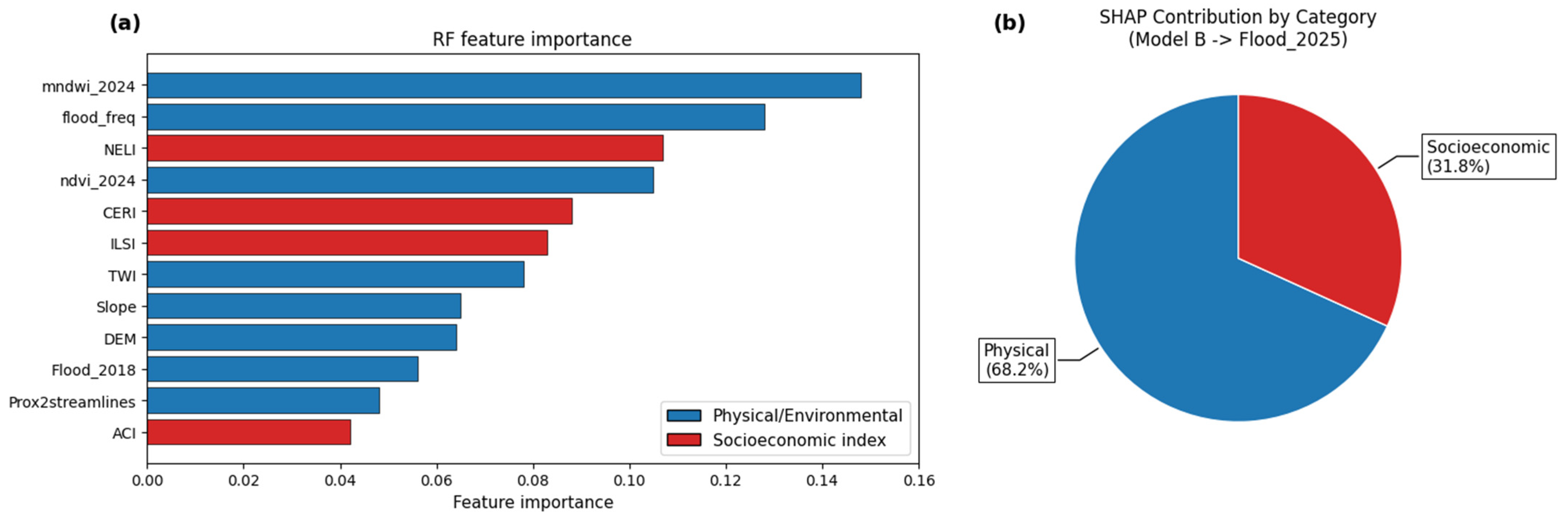
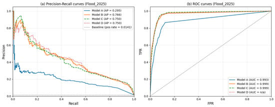
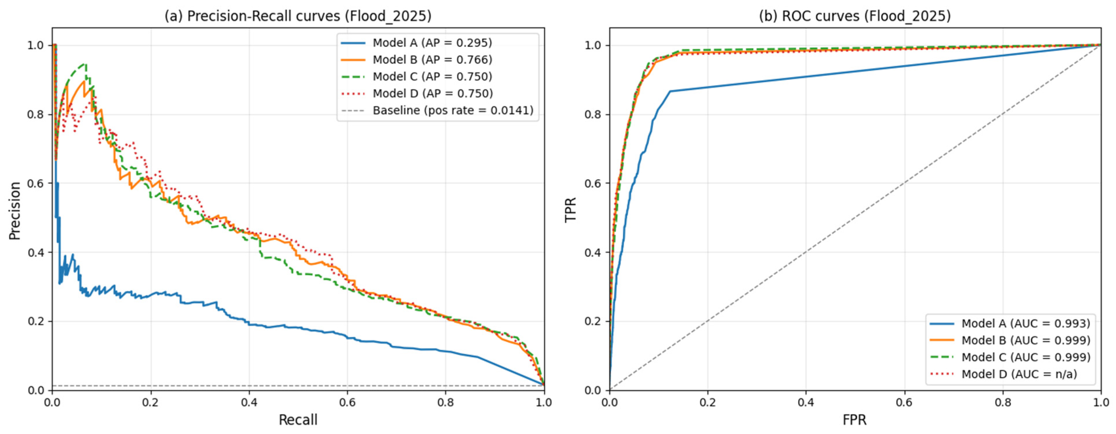
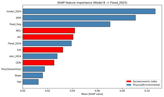
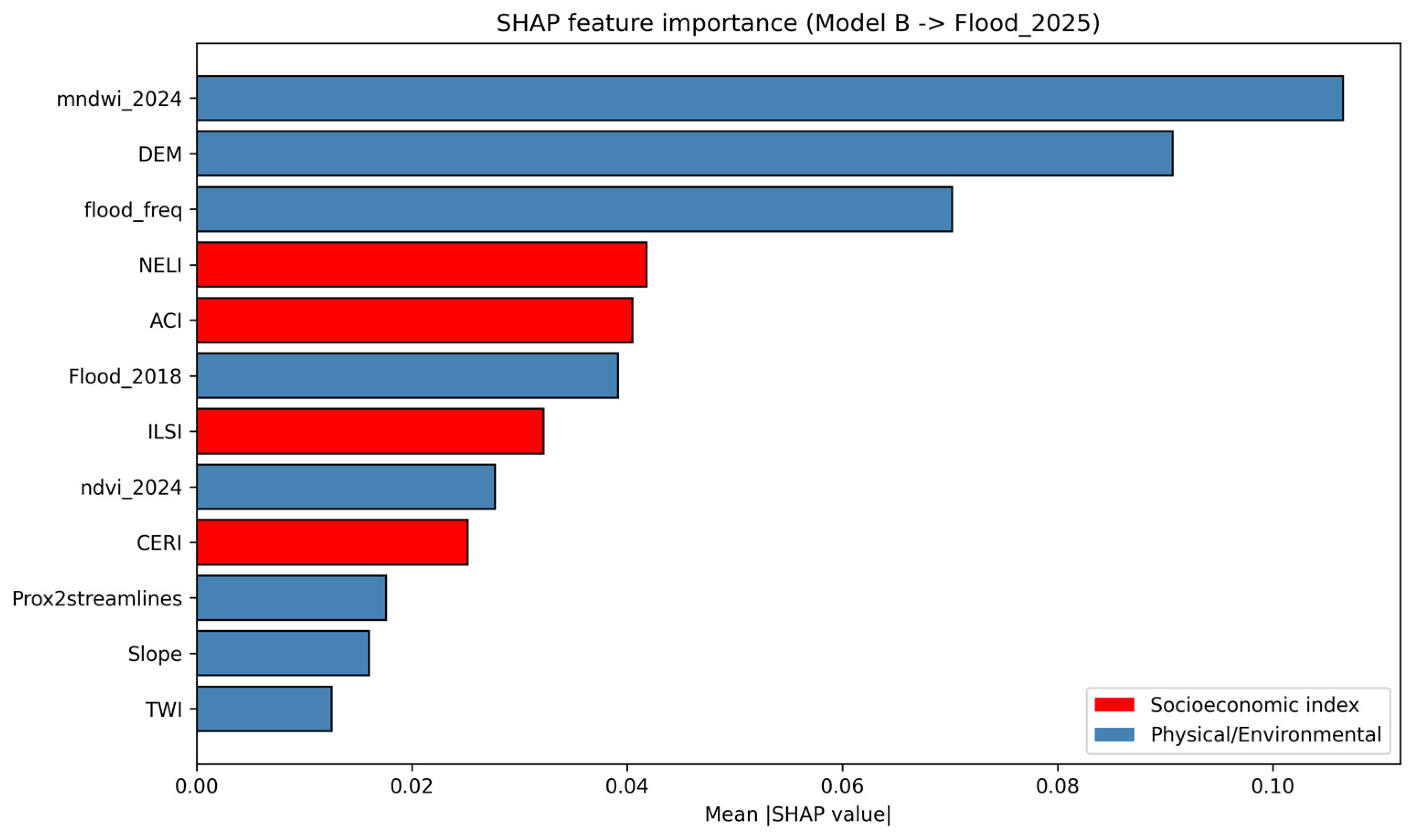
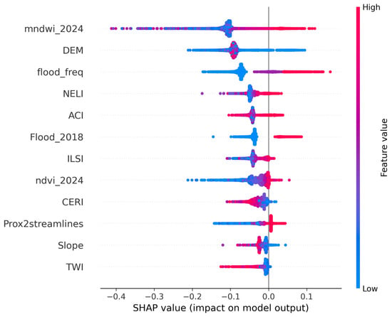
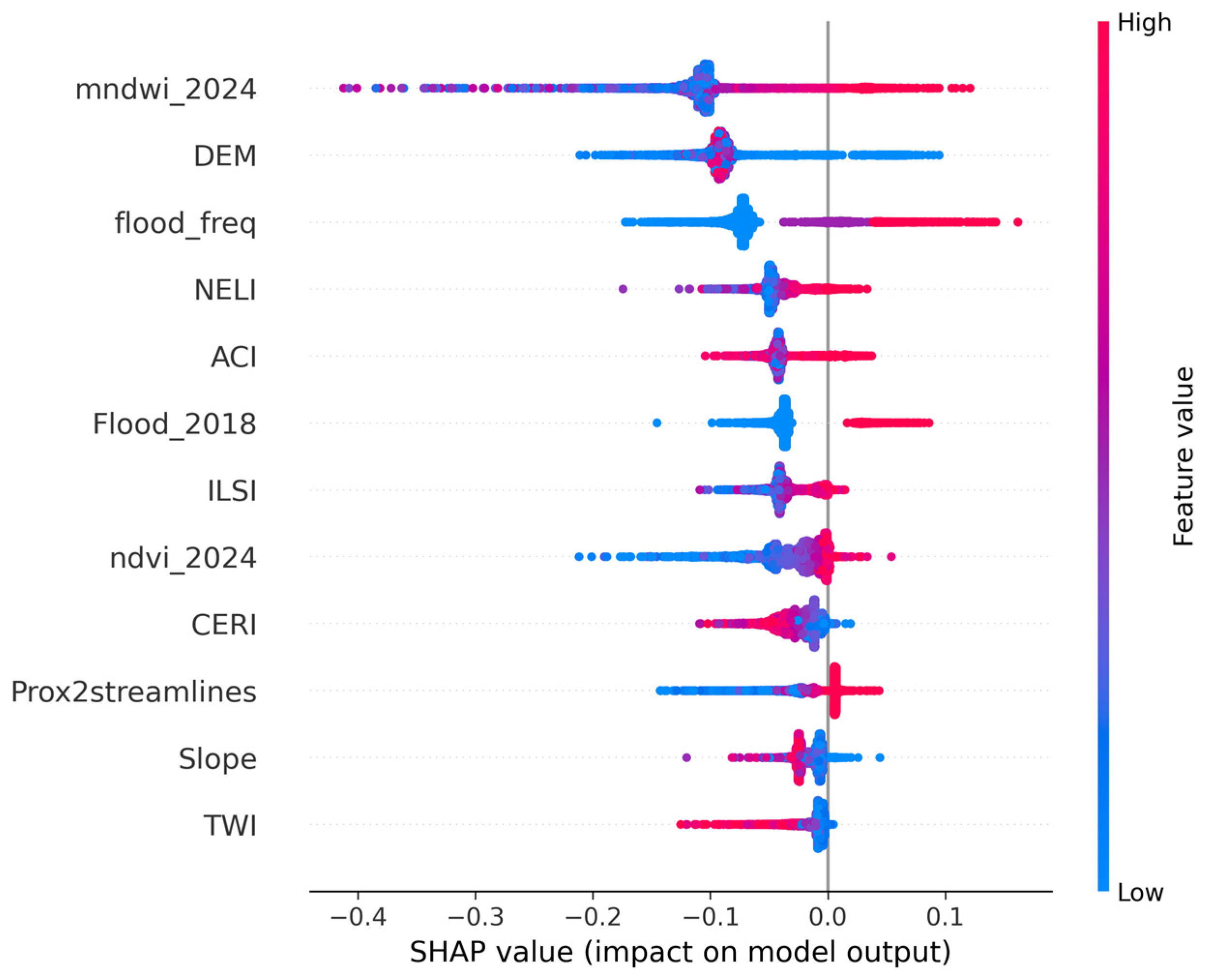
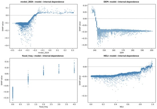
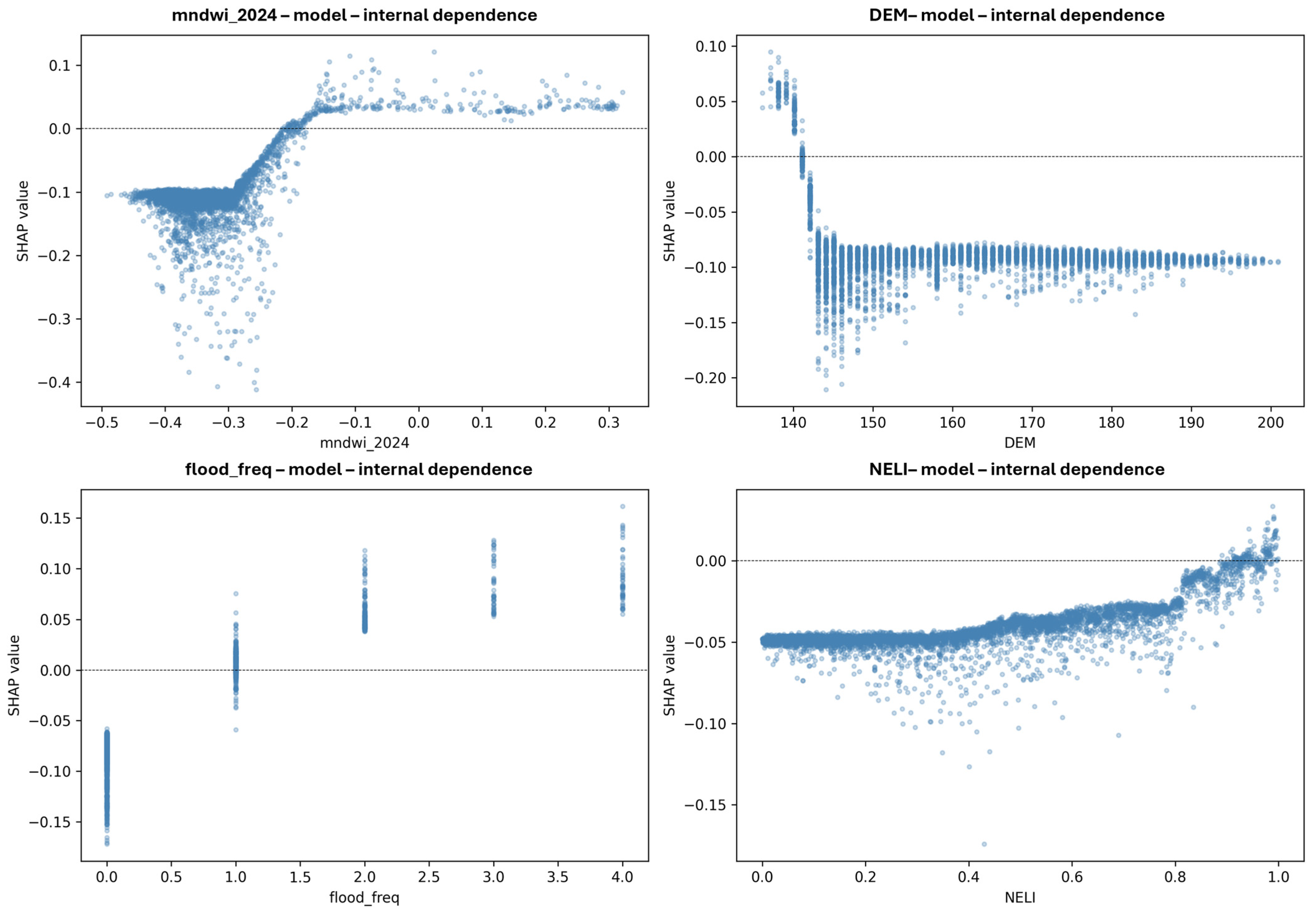
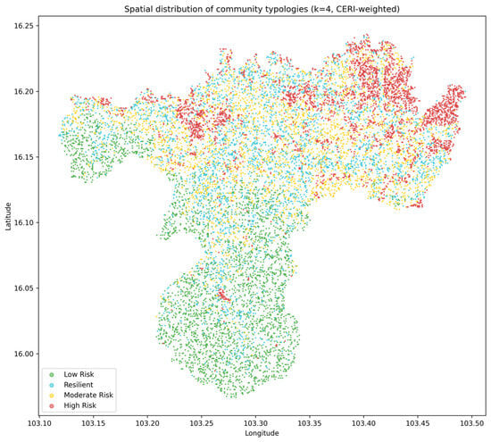
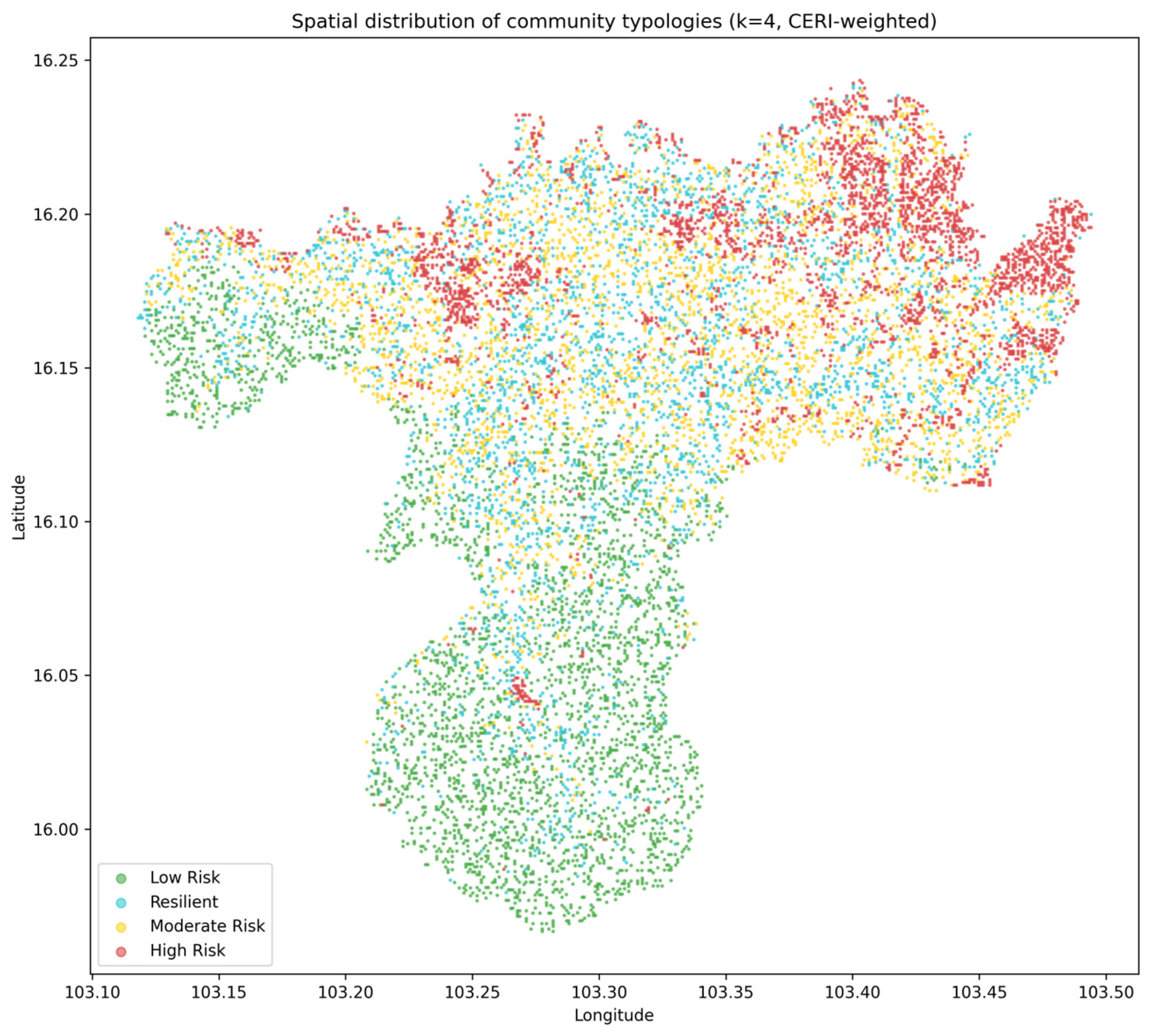
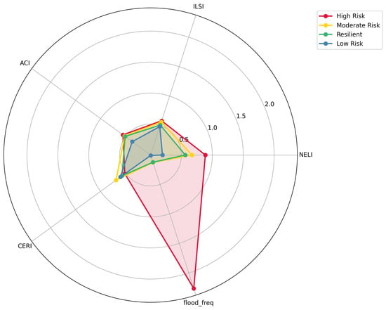
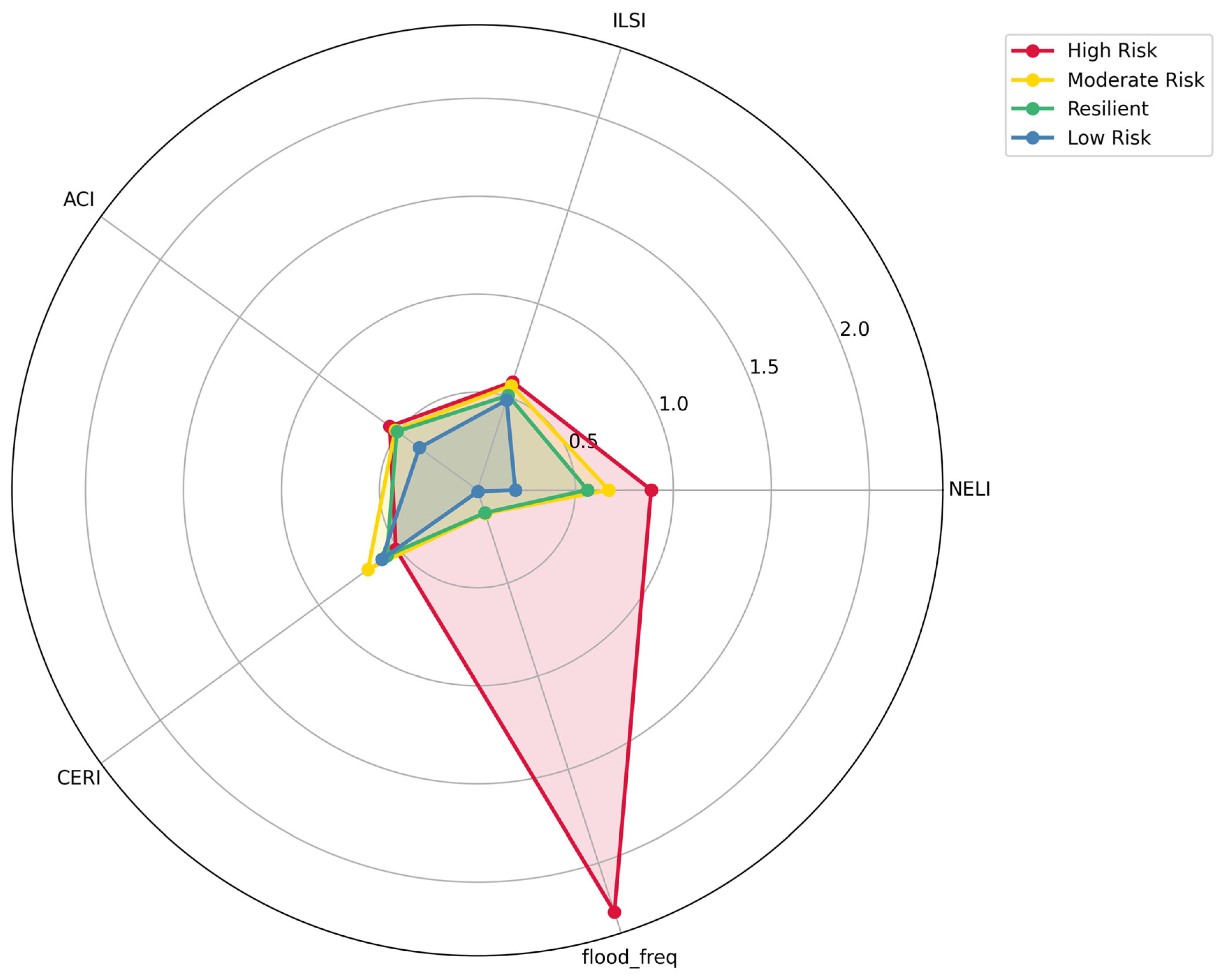
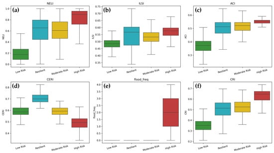
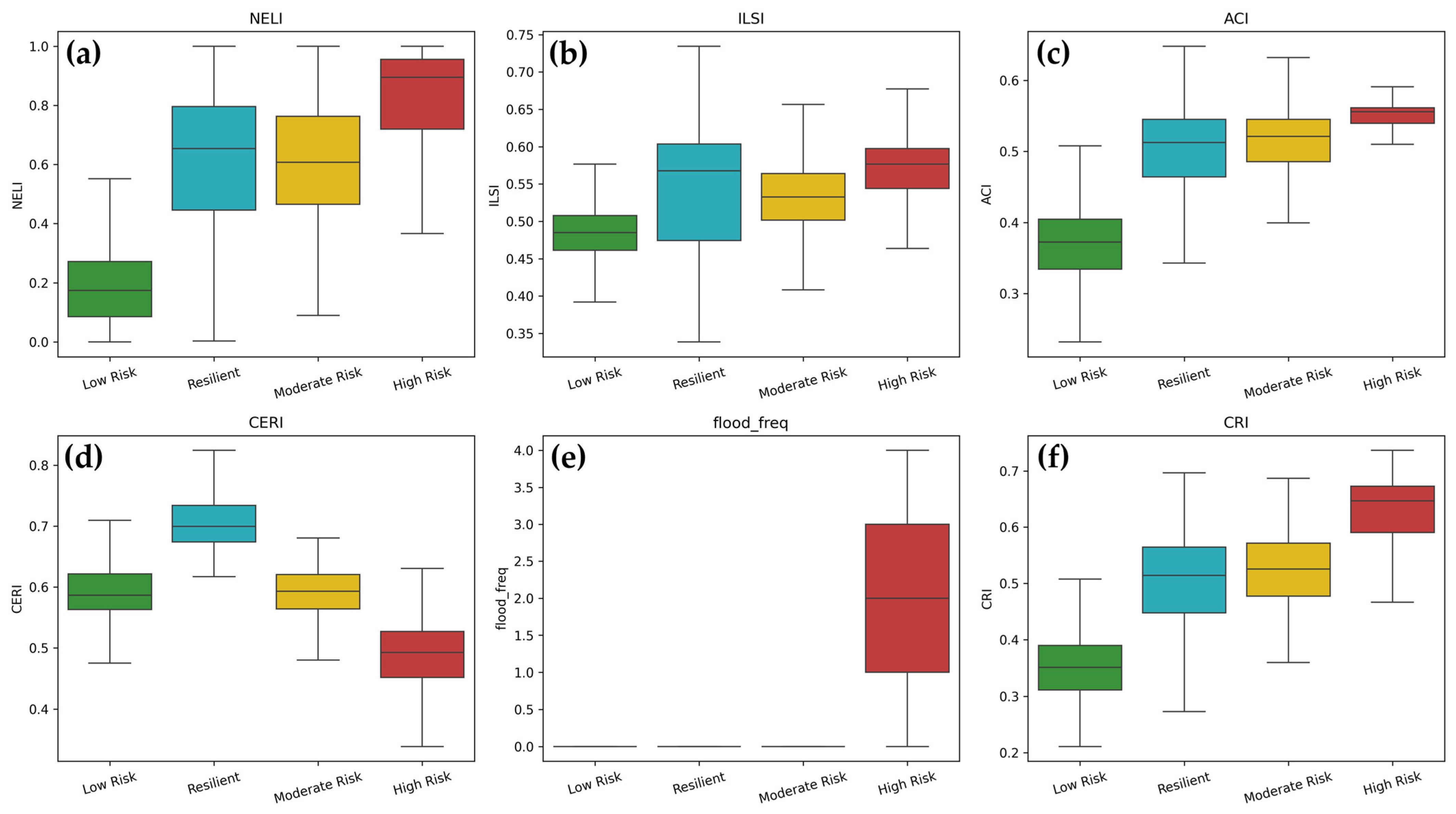
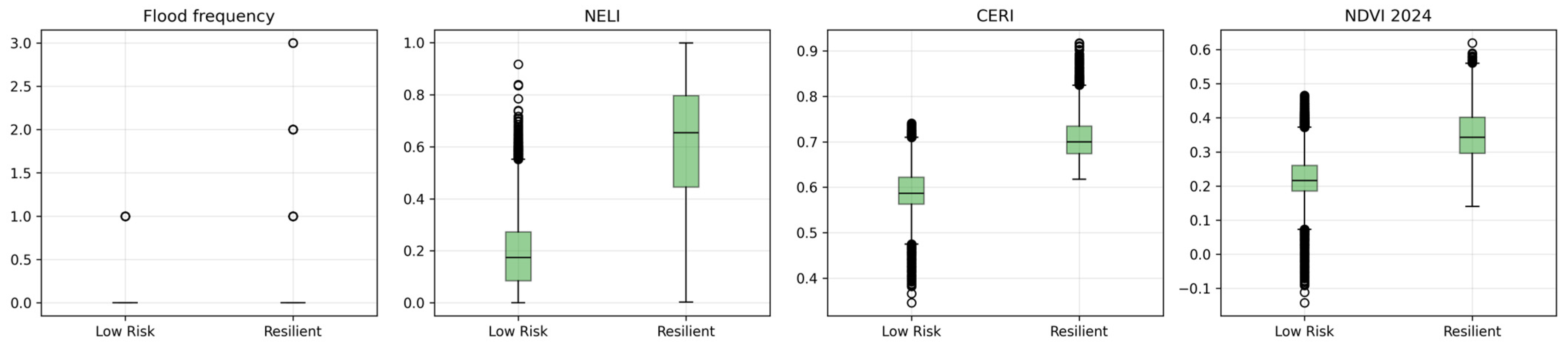
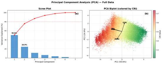
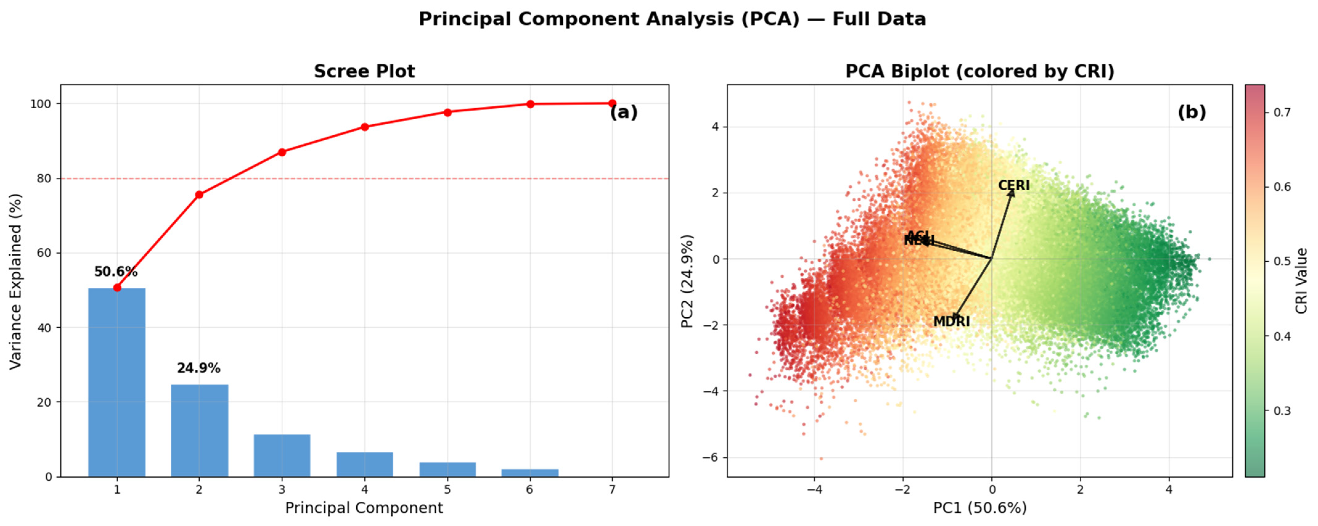

Disclaimer/Publisher’s Note: The statements, opinions and data contained in all publications are solely those of the individual author(s) and contributor(s) and not of MDPI and/or the editor(s). MDPI and/or the editor(s) disclaim responsibility for any injury to people or property resulting from any ideas, methods, instructions or products referred to in the content. |
© 2026 by the authors. Licensee MDPI, Basel, Switzerland. This article is an open access article distributed under the terms and conditions of the Creative Commons Attribution (CC BY) license.