


Abstract
Climate conditions affect the macroeconomic and financial environment, which in turn affects sustainable agricultural development in South Africa. In this study, the short- and long-run relationships between agricultural performance, temperature, economic activity, trade openness, Consumer Price Index and financial-sector development are investigated using annual South African time-series data for the period 1972 to 2022 in an ARDL (Autoregressive Distributed Lag) model. The ARDL bounds test confirms a long-run equilibrium relationship among the variables included in the final specification. Economic activity exhibits a negative and statistically significant long-run association with agricultural performance (β = −0.7985, p = 0.0009). Temperature also has a negative long-run coefficient (β = –0.1119), but this is not statistically significant at conventional levels (p = 0.1212). In addition, financial-sector development has a negative, but marginally significant association with agricultural performance (β = −0.0032, p = 0.0589), whereas the natural logarithm of the Consumer Price Index (β = 0.3994, p = 0.0537) and trade openness (β = 0.0080, p = 0.0873) have positive, but marginally significant associations. The sign of the error correction coefficient is negative and highly significant (−0.4742, p < 0.001), suggesting that around 47.4% of short-run disequilibria will be resolved over a period of a year. Overall, the results indicate that agricultural performance is linked with climatic, macroeconomic, trade, and financial conditions in South Africa. However, the strength and statistical significance of these relationships vary across variables. The results therefore provide evidence relevant to sustainable agricultural development while supporting careful consideration of climate adaptation, macroeconomic stability, productive finance, and market integration.
1. Introduction
Climate change is a major structural problem for the socioeconomic sustainability of agriculture and food systems in developing economies. The increasing frequency of climatic hazards such as droughts, heat waves, unpredictable rainfall patterns, and environmental degradation poses production and food-security risks for agriculture, especially in African economies, where agricultural production is highly vulnerable to climatic conditions. The impact on macroeconomic growth or performance can also stem from reduced productivity, food price volatility, labour market disruption, and reduced sectoral resilience due to climate-related events [1,2]. Climate change is therefore becoming well recognised not only as an environmental risk but also as a risk to systemic development, including macroeconomic and ecological development.
The SA also underwent large-scale structural transformation over the past few decades, during which the share of agriculture in aggregate productivity and employment has declined, while service sector activities have grown in relative significance and financial services have expanded. The developments pose important challenges, as agricultural production is also under pressure from climatic conditions and broader macroeconomic and sectoral adjustment processes. Structural economic change can mean structural change in agricultural investment, in the allocation of labour in agriculture, in access to productive finance, and in the allocation of resources that affect agricultural sectors, and the shocks of climate change can worsen food insecurity and agricultural productivity. Therefore, to appreciate agricultural performance, it must be considered within a broader development context that incorporates environmental and economic pressures.
Agricultural systems’ independence is also closely tied to macroeconomic developments through various transmission channels. Inflation affects agricultural input prices, profit and purchasing power, and openness to trade in agricultural markets, export opportunities, import competitors, and international price volatility. Likewise, financial sector development may influence agricultural performance through credit availability, investment, financial inclusion, and access to investment in productive resources. While financial deepening can facilitate agricultural development, expanding the financial sector does not necessarily mean that financial resources will be allocated towards agriculture, especially if these resources are concentrated in urban and non-agricultural activities [3,4].
Although there is an increasing number of publications on climate change and farming, important empirical gaps remain. Existing studies have analysed the direct relationship between climate and agricultural processes, explored agricultural vulnerability, adaptation behaviour, or agriculture-specific responses. At the same time, comparatively less research has examined the linkages between climate, macroeconomic processes, financial-sector growth, and agriculture within an empirical framework. The restriction is significant in the South African context. It is particularly relevant given the relatively few South African studies that employ dynamic time-series methods to identify long-run equilibrium relationships from short-run adjustment processes.
Therefore, the focus of this study is to analyse the relationships among temperature, economic activity, inflation, financial sector development, trade openness, and agricultural performance in South Africa. Rainfall is considered within the broader climatic framework, while the variables retained in the final ARDL specification are reported explicitly in the empirical methodology. For the analysis, Pesaran et al. [5] suggested using the Autoregressive Distributed Lag (ARDL) model, which is suitable when the variables involved have mixed orders, I(0) and I(1). Still, none is I(2), or double-integrated. The ARDL approach also allows estimation of long-run relationships and short-run dynamics within a single econometric framework.
Accordingly, the study addresses the following central research question: How are climatic conditions, macroeconomic dynamics, and financial-sector development associated with agricultural performance in South Africa in the short and long run? In particular, the analysis addresses whether short- and long-run features of climate, economic activity, inflation, financial sector development, and trade are related to agricultural performance. The analysis focuses on whether, on the one hand, the short- and long-run dynamics of climate and selected macroeconomic variables are related to agricultural performance, and, on the other hand, whether they contain predictive information for agricultural performance. Structural transformation is not used as an empirical dimension but as a theoretical development environment.
2. Literature Review
2.1. Theoretical Framework
In the study’s conceptual framework, three complementary theories are investigated: climate–macroeconomic risk theory, structural transformation theory, and financial intermediation theory. Together, these theories offer a conceptual framework for understanding how climate-induced adverse shocks affect the agricultural sector’s performance through macroeconomic, sectoral, and financial transmission channels in the South African economy.
2.1.1. Climate–Macroeconomic Risk Theory
Climate–macroeconomic risk theory explains how climate change shocks can trigger broader macroeconomic shocks through interconnectedness among employment, productivity, inflation, trade, and financial systems. In recent years, climate change has gained new significance in economics as a systemic macroeconomic risk that can affect economic performance, agricultural productivity, and long-term development outcomes [1].
Empirical studies have shown that climate shocks, such as rising temperatures, rainfall variability, environmental degradation, and extreme weather events, affect climate-sensitive industries, such as agriculture and energy, disproportionately, especially in developing economies, where structural instability and limited adaptive capacities are severe [1]. This, in turn, results in the forfeiture of output growth, inflation, food insecurity, and macroeconomic instability.
One of the main pathways between climate change and agricultural productivity is through reduced productivity. Author [6] states that higher temperatures significantly reduce labour productivity and output, with particularly severe consequences in climate-sensitive industries such as agriculture and construction. Climate shocks also affect the inflation process and financial conditions through supply shocks. Temperature shocks can adversely affect economic growth and agricultural productivity, particularly in developing economies, thereby contributing to broader macroeconomic vulnerabilities [7]. In this sense, climate-induced shocks increasingly serve as macroeconomic transmission channels that affect sectoral and overall economic outcomes. Climate–macroeconomic risk theory as a whole offers a helpful framework for understanding how climate shocks trigger adjustment processes across productivity, inflation, output, trade, and the financial sector.
2.1.2. Structural Transformation Theory
The long-run shift in economic activity from agriculture to manufacturing and services during economic development is explained by the structural transformation theory. The theory is mainly attributed to [8,9], who claim that economic growth normally observes a diminishing contribution by agriculture to the gross domestic product (GDP), as there is a steady movement of labour and capital from agriculture to other sectors of the economy that use less of these factors.
The dual-sector model, proposed by [8], addresses the shift in labour from the traditional, low-productivity agricultural sector to the modern, high-productivity industrial sector, facilitated by capital accumulation. Similarly [9] suggests that during economic development, there will be a structural transformation, which entails sectoral reallocation, urbanisation, technological progress, and changes in production structures.
While structural transformation can certainly increase economic growth in the longer term, it can also cause agricultural decline if investment, productivity and institutional support for the agricultural sector decline during economic transition. The present study applies structural transformation theory within a broader context to interpret changes in the economic landscape surrounding agriculture. The results of the empirical model in the present paper are therefore interpreted at the macro level, not as a measure of structural transformation or sectoral reallocation per se in practical terms, though they do represent economic activity.
2.1.3. Financial Intermediation Theory
The Financial Intermediation Theory encompasses Financial Institutions and explains how they mobilise savings, allocate credit, manage risk, and facilitate economically productive activity. According to conventional financial theory, the purpose of a financial intermediary is to increase economic efficiency by reducing transaction costs, solving information problems, facilitating the smooth transformation of liquidity, and allocating capital.
According to a systematic review by [10], financial intermediation is a multidimensional activity that entails credit allocation, financial inclusion, liquidity transformation, and systemic risk management. Financial intermediation is significant in the agricultural system with respect to farm investment, technology adoption, irrigation, agricultural inputs, and capacity for climate adaptation.
Author [11] stated that it is an extension of the theory of financial intermediation, incorporating banking-sector liabilities, liquidity conditions, and financial confidence in macroeconomic adjustment processes. Financial systems could thus be indirectly affected by climate-related shocks through changes in repayment conditions, collateral quality, financial uncertainty, and systemic vulnerability.
Agricultural sectors in developing economies are often exposed to weak, limited access to productive finance due to high climate risk, limited collateral, and uncertainty about agricultural returns. Thus, financial development alone cannot guarantee an increase in agricultural productivity unless its supply is focused on agriculture.
The broader theory consequently informs understanding of the potential association between financial-sector development and agricultural performance in South Africa. When a negative correlation is observed in practice, potential explanations include financial exclusion, differences in credit allocation across sectors, restricted agricultural financing, or other institutional barriers. The mechanisms are considered potential, not actual effects directly observed using the estimated financial-development coefficient.
2.1.4. Integrated Theoretical Framework
Climate–macroeconomic risk theory, structural transformation theory, and financial intermediation theory are integrated into a single analytical framework to explain how climate-related shocks affect agricultural performance through macroeconomic, structural, and financial transmission channels.
Climate variables such as temperature and rainfall variability are external shocks conceptualised within the framework that will initially affect agricultural productivity and output conditions. The effects of climate disruptions then lead to macroeconomic pressures, including inflation, instability, reduced productivity, food insecurity, and trade disruptions. Agricultural performance might also decline further due to the dynamics of structural transformation, as labour, investment, and financial resources are transferred to the industrial and service sectors.
These macroeconomic and structural changes, in turn, affect financial conditions through shifts in credit allocation, agricultural financing, financial inclusion, and systemic uncertainty. As such, amid macroeconomic instability and climate change, agriculture could lose productivity and investment support, becoming more susceptible to financial exclusion.
The integrated framework separates variables that are estimated in the empirical model from those that address theoretical transmission mechanisms. Structural transformation theory provides the broader theoretical context; however, LGDP is treated empirically as a proxy for aggregate economic activity rather than as a direct measure of structural transformation or sectoral reallocation. The climatic variables considered in the conceptual framework include temperature and rainfall; however, the variables retained in the final estimated ARDL specification are identified explicitly in Section 3. Figure 1 illustrates the integrated conceptual framework linking climatic conditions, macroeconomic dynamics, financial-sector development, and agricultural performance in South Africa.
Figure 1.
Conceptual framework linking climatic, macroeconomic and financial dynamics to agricultural performance in South Africa. Source: Authors’ construction based on [1,8,9,11]. Note: The conceptual framework illustrates the theoretical channels through which climatic conditions, macroeconomic dynamics, structural economic processes, and financial-sector conditions may interact with agricultural performance in South Africa. Structural transformation is treated as a broader theoretical development context rather than as a directly measured empirical variable. The variables retained in the final ARDL specification are reported explicitly in Section 3.
2.2. Empirical Literature
2.2.1. Climate Change and Agricultural Performance
A range of empirical literature confirms that climate change impacts on agriculture are manifested in increased temperatures, greater rainfall variability, increased drought frequency, heat stress, and changes in extreme weather events. Agricultural vulnerability is evident in South Africa, especially in areas where low irrigation intensity, high exposure to climate shocks, land degradation, and low adaptive capacity make small-scale farming vulnerable. According to Author [12], for instance, the KwaZulu-Natal Midlands is a climate change hotspot, as agricultural systems are highly vulnerable to climate variability and have limited margins for adaptation due to a lack of infrastructure, income, and irrigation facilities.
The same can be seen throughout much of Sub-Saharan Africa, where agriculture is highly reliant on rainfall and thus highly exposed to climate variability. Author [2] demonstrates that changes in temperature and rainfall lead to reduced agricultural production and a shorter growing season across the region. Similarly, Author [13] identifies frequent challenges faced by farmers, including changing rainfall patterns and reduced crop productivity, indicating that rainfall uncertainty remains one of the biggest challenges affecting agricultural production in climate-exposed economies.
The temperature channel is equally important, too. Authors [6] show that in exposed agricultural sectors, exceeding 32 °C has substantially negative effects on labour supply; more broadly, empirical evidence suggests that heat exposure depresses agricultural yields, diminishes labour productivity, and creates uncertainty in the agricultural production of climate-vulnerable crop sectors. Studies conducted in developing countries also indicate that rising temperatures and changes in precipitation patterns may adversely affect agricultural yields, particularly for climate-sensitive crops such as maize, millet, and sorghum [14,15].
But literature also indicates that climate impacts can be non-linear and heterogeneous. Others report differences across crops, with some benefiting or even increasing yield under specific climate scenarios and others seeing significant decreases in productivity [16,17]. This indicates that an understanding of agro-ecological conditions, technological adaptation capabilities, institutional support, irrigation availability, and crop type is all-important in determining agricultural responses to climate change.
For South Africa specifically, Shoko et al. [18] provide an important benchmark by studying the impact of climatic conditions on maize production using an ARDL-ECM approach. The study they conducted illustrates how temperature, precipitation, and other production variables affect crop performance. The empirical scope of the present study is broader because it assesses overall agricultural performance rather than a particular crop, and synthesises climatic variables with macroeconomic and financial variables within a broader dynamic framework. The contribution also differs from traditional climate–crop relationship models by investigating whether agricultural performance is part of a wider system of adaptation to climate change under macro-financial constraints.
2.2.2. Structural Transformation and Agricultural Performance
There is a strong link between structural transformation and the relationship between economic growth and agricultural performance. There is strong evidence that as economies grow, labour, capital, and investment are more likely to be drawn from the agricultural sector to the manufacturing and service sectors. Such a shift can reduce agriculture’s relative importance in the economy, even though it is a key component of food security and rural livelihoods.
Recent work on structural transformation highlights the role of sectoral reallocation, human capital development, technological upgrading and productivity improvement for long-run economic growth. Author [19] illustrates the critical role of structural change and human capital development in productivity and competitiveness in emerging economies. In the same vein, research on South Africa’s sectoral transformation calls for integrated policy interventions that focus on infrastructure, skills, energy constraints, and sectoral diversification. The present study investigates agricultural adjustment within the broader development context of this literature; however, economic growth is not seen as a direct measure of structural transformation. LGDP is thus not seen as a simple measure of reallocation of resources by sector but as an indirect measure of reallocation of resources derived through the mechanism of economic activity.
2.2.3. Financial Development, Credit Constraints and Agriculture
It is well known that financial development can foster agricultural productivity and enable farmers to invest in agricultural practices such as irrigation, climate-resilient technologies, mechanisation, and market access. The literature reviewed from various sources indicates that access to agricultural credit improves farm productivity, technology adoption, and household income. Still, these improvements may not be evenly distributed across gender, income, and farm-size groups [20,21].
But the links between financial development and agricultural performance are complex. A number of the challenges that agricultural producers in developing countries face include ongoing credit constraints tied to collateral requirements, perceived climate risk, financial literacy, banking infrastructure, and institutional barriers. In their systematic review of developing and underdeveloped countries, authors [3] indicate that farmers face various barriers to accessing formal credit and productive assets. By the same token [4], highlights certain constraints on access to agricultural credit in Africa, including information asymmetry, input prices, lack of cooperative membership, and poor rural infrastructure.
There is also evidence from South Africa and other developing countries that financial exclusion is a significant impediment to agricultural transformation. While the use of digital financial services and fintech products promises to enhance financial inclusion in agriculture, this relies on digital infrastructure, policy coordination, financial literacy, and institutional capacity [22,23]. Author [24] also reveals that informal financial institutions are often utilised by rural populations, as the formal financial system is largely urban-oriented.
This is a significant empirical lacuna. Many studies examine the link between credit access and agricultural productivity at the individual household or farm level. Still, few examine the aggregate relationship between financial sector development and agriculture within a macroeconomic time-series framework. The present study seeks to fill this gap by analysing financial development alongside climate and macroeconomic variables.
2.2.4. Macroeconomic Transmission: Inflation, Trade and Agricultural Output
Agricultural performance could also be affected by other macroeconomic indicators, such as inflation and openness to trade. There are incentive and cost effects of inflation on agriculture. Agricultural prices can be used to increase producer incentives and income, but can also be an inflationary factor in production. Inflation increases the production costs of inputs such as fertiliser, fuel, transport, machinery, and labour, thereby reducing production capacity and profitability.
Existing literature has demonstrated that inflationary pressures stemming from climate shocks, currency instability, rising fuel prices, and food supply challenges significantly affect agriculture. Furthermore [25] demonstrates that exchange rate depreciation and inflation had a positive impact on food prices, which in turn increased input prices and affected smallholder farmers in Nigeria. The influence of climate change on food availability, accessibility, and affordability has also been documented by the author [2], who reports decreased yields and shorter growing seasons for food crops in Sub-Saharan Africa. These studies corroborate the perception that agriculture is both environmentally sensitive and vulnerable to macroeconomic instability.
The impact of trade openness on agriculture is also ambivalent. Trade openness may also foster greater access to technology and inputs, as well as competitiveness and market access. Some disadvantages are that it can make domestic producers vulnerable to international price volatility, import competition, exchange rate fluctuations, and external shocks. The literature on the link between trade openness and food security remains sparse and largely lacks causal analysis, as author [26] points out. Author [27] highlights the nature of the impact that trade liberalisation could have on agriculture through scale, structural, transport, and technology effects.
2.2.5. South African Context and Empirical Gap
South Africa is a relevant country for analysing the performance of the agricultural sector, its economic and social roles amid climate change and structural transformation, as agriculture remains one of the most important sectors in the country despite its small share of GDP. Uncontrollable factors such as rising temperatures, variability in rainfall, drought events, water scarcity, land degradation, and unequal access to adaptation infrastructure pose risks to the sector. Meanwhile, farmers operate within a structurally changing economy characterised by financial deepening, urbanisation, rising energy costs, and persistent inequality.
There was valuable information on climate vulnerability, agricultural adaptation, conservation agriculture, climate-smart agriculture, and extension services in the existing SA literature. Authors [28] describe the fragility of smallholders in the climate-sensitive zone, and [29] highlight the benefits of conservation and climate-smart agriculture for smallholder adaptation. But the current literature is more geared towards adaptation practices, vulnerability assessment and resilience at the farm level rather than the transmission mechanisms at the macro level.
The present study is motivated by three related gaps: Empirically, the majority of previous South African studies have focused on direct climate–agriculture interactions, crop-specific responses, farm-/agricultural-system vulnerability, or the response of agricultural systems to climate change—with limited studies looking at the combined link between aggregate agricultural performance and climatic, macroeconomic, trade and finance conditions. ARDL-ECM method approaches have been applied to specific agricultural outcomes in South Africa, including crop-level analyses; however, comparatively limited research has jointly examined climatic, macroeconomic, trade, and financial variables within a single dynamic specification that distinguishes long-run equilibrium relationships from short-run adjustment processes. On a substantive basis, there is little evidence in the literature of a debate between interpreting agricultural vulnerability as a climate-production issue and viewing it as part of a wider climate–macro-financial adjustment system relevant to sustainable development. In this regard, the present study fills these gaps by integrating agricultural performance into a unified dynamic model and examining variables estimated directly, as well as those implicit in the broader model of agricultural development mechanisms, such as structural transformation.
3. Data and Methods
3.1. Research Design
The research design for this study employs a quantitative approach, drawing on time-series econometric methods to examine the relationships among climate change, structural change, and agricultural performance in South Africa. The use of a quantitative design is suitable, as it aims to examine the relationship between macroeconomic and climatic parameters using annual secondary data over time. The method provides an estimate of short-run dynamic adjustments and long-run equilibrium relationships between the variables of interest.
Additionally, the study utilised an explanatory design. It analysed the dynamic links among climatic conditions, macroeconomic variables, the development of the financial sector, and the performance of the agricultural sector in the South African economy. Specifically, the analysis considers economic activity, financial sector development, trade openness, the inflation rate, and temperature and rainfall conditions in relation to agricultural output. The estimated relationships are interpreted as conditional short-run and long-run associations rather than structural causal relationships.
3.2. South African Economic Context
This study must focus on South Africa, a developing economy with significant climatic variability, structural change, and sectoral inequalities. South Africa is an appropriate case study for analysing climate-sensitive agriculture, as agriculture is highly vulnerable and sensitive to rising temperatures, rainfall fluctuations, droughts, water scarcity, and environmental degradation. Furthermore, reliance on rain-fed agricultural production systems increases the vulnerability of crops to climate-driven productivity shocks [30].
Agriculture is an important sector, with a relatively low share of Gross Domestic Product (GDP) but a significant role in food production, rural livelihoods, agro-processing industries, export earnings, and employment generation. South Africa’s agriculture remains highly dependent on the climate, yet several instances of instability render agricultural production vulnerable to climatic variability. Preliminary studies also indicate that inter-provincial climate shock differences are present, leading to bi-modal climate regions and scope for inter-provincial climate shock differences that worsen agricultural productivity and rural vulnerability differences [31]. The geographical context of the study area is illustrated in Figure 2.
Figure 2.
Study area map of South Africa. Source: Authors’ construction using public-domain geographic boundary data from Natural Earth. This map shows the Geographical area of South Africa, its provinces, neighbouring countries and some major South African cities. Natural Earth vector geographic data are made freely available and can be copied and modified without any special copyright permissions.
3.3. Data Sources
The data in this study consist of annual secondary time series for South Africa over 51 years (1972–2022). Actually, the effective sample size varies across econometric procedures due to data availability and adjustments to lag structures and differencing requirements. EViews 12 automatically adjusts the estimation sample based on the lag specifications specified in the manuscript and the number of observations available for each procedure. As a result, the number of observations used in the descriptive analysis can differ from that used in the unit-root tests and ARDL estimation. The information comes from the World Bank’s World Development Indicators and World Bank Climate Change Knowledge Portal, which provide data on agricultural performance, climatic conditions, macroeconomic variables, trade openness, and financial sector development. EViews is used for the empirical analysis.
Agricultural performance, abbreviated as LNAGRI, is measured by taking the logarithm of agricultural output. This output includes production from agriculture, forestry and fisheries. The basic agricultural series is a measure of output from the agricultural sector, and it is converted to natural logarithms before the estimation. Temperature, abbreviated as TEMP, is measured as the annual surface air temperature in degrees Celsius. Rainfall, abbreviated as RF, is measured as the annual precipitation in millimetres. These climatic series are used to show the temperature and rainfall conditions that affect agricultural production in South Africa.
Economic activity, abbreviated as LGDP, is measured by taking the logarithm of Gross Domestic Product. Since agricultural activity contributes to aggregate GDP, including LGDP alongside agricultural output introduces a potential part–whole relationship. Therefore, the estimated relationship between economic activity and agricultural performance is interpreted cautiously and does not, by itself, establish sectoral reallocation or structural transformation. The sensitivity of this relationship to alternative measures of economic activity is a consideration for the robustness of the empirical specification. LGDP is used to represent economic activity rather than as a direct measure of structural transformation. Trade openness, abbreviated as TO, is measured by dividing the sum of exports and imports by GDP. It is shown as a percentage of GDP. Financial sector development, abbreviated as FS, is measured by credit extended to the private sector as a percentage of GDP. FS shows how much credit financial institutions extend to the sector relative to the economy’s size.
The consumer-price variable, abbreviated as LCPI, is defined as the logarithm of the Consumer Price Index. The CPI shows the level of consumer prices and is therefore different from the annual inflation rate. The natural logarithm transformations used for LNAGRI, LGDP, and LCPI are kept the same as those used for the model variables.
3.4. Variable Description and Measurement
Table 1 shows that temperature and annual rainfall are included to capture climatic conditions relevant to agricultural production, particularly through heat stress, water availability, crop performance, and production stability. Economic activity is included based on its association with the broader macroeconomic environment for South Africa’s development. Nevertheless, LGDP is not taken as a direct indicator of structural change or sectoral reallocation; aggregate economic activity can be understood in this context. The structural transformation theory thus does not claim to be an empirical proxy, but rather offers an interpretation. Trade openness reflects the degree of integration with international markets. At the same time, the Consumer Price Index represents the general consumer price level, which may be linked with agricultural production costs, market conditions, and profitability. Financial-sector development is proxied by domestic credit to the private sector as a percentage of GDP, capturing the relative scale of private-sector credit provision rather than the full breadth or institutional development of the financial system.
Table 1.
Study Variables, Measurement, and Expected Relationships.
3.5. Model Specification
The functional model is expressed as follows:
LNAGRIt = f(TEMPt, RFt, LGDPt, TOt, FSt, LCPIt)
The econometric model is specified as
where
LNAGRIt = β0 + β1TEMPt + β2RFt + β3LGDPt + β4TOt + β5FSt + β6LCPIt + εt
- LNAGRIt = Natural logarithm (ln) of agricultural output
- TEMPt = Temperature
- RFt = Annual rainfall
- LGDPt = Logarithm of Gross Domestic Product Products
- TOt = Trade openness
- FSt = Financial-sector development
- LCPIt = Logarithm of the Consumer Price Index
- εt = Error term
The ARDL error-correction representation is specified as follows:
where
- Δ = First-difference operator
- ECTt−1 = Error-correction term
- λ = Speed of adjustment parameter
- μt = White-noise error term
Rainfall (RF) and temperature (TEMP) were initially incorporated into the model to capture climatic conditions influencing agricultural performance. However, their inclusion raised concerns regarding potential multicollinearity, as both variables reflect related dimensions of climatic variability. Consequently, rainfall was excluded from the final ARDL specification to address these concerns. At the same time, temperature was retained alongside economic activity (LGDP), trade openness (TO), financial sector development (FS), and the consumer price index (LCPI). This specification decision does not diminish the theoretical importance of rainfall but reflects the methodological considerations associated with the preliminary model estimation.
3.6. Estimation Procedure
Descriptive analysis, stationarity test, lag-length selection, cointegration test, long-run estimation, short-run estimation, diagnostic test, and causality test are adopted as a systematic econometric analysis procedure in the empirical analysis. The evaluation of statistical inference at the 1%, 5% and 10% levels. Thus, coefficients with p-values < 0.01, 0.05 and 0.10 are deemed statistically significant at the 1%, 5% and 10% levels, respectively. Results significant at the 10% level are simply described as ‘marginally significant’ to clearly differentiate them from the level of significance of 1% and 5%.
3.6.1. Descriptive Statistics Procedure
To summarise the characteristics of the variables, descriptive statistics such as the mean, median, standard deviation, skewness, kurtosis, and Jarque–Bera statistics are first used [32,33].
3.6.2. Unit Root Tests
To assess whether variables are stationary, this study uses the Augmented Dickey–Fuller (ADF) and Phillips–Perron (PP) tests [34]. The ARDL methodology requires that variables be integrated of order zero (I(0)) or order one (I(1)), but not of order two (I(2)).
The ADF equation is represented as
The Phillips–Perron equation is represented as
Yt = β0 + β1Yt−1 + μt
Before applying the ARDL bounds-testing approach, the variables’ integration properties were assessed using the ADF and PP tests. Both tests were applied to assess stationarity at the level and first-difference levels, and the statistical significance was assessed at the 1%, 5% and 10% levels. If the tests did not agree, the interpretations were based on each test’s significance level. The ARDL bounds-testing approach allows for the inclusion of I(0) and I(1) variables, but no variable to be integrated of order I(2).
3.6.3. Lag Length Selection
The Akaike Information Criterion (AIC), Schwarz Information Criterion (SC), and Hannan–Quinn Information Criterion (HQ) [35,36] were used to evaluate the optimum lag length. The preliminary Vector Autoregression (VAR) lag-order selection procedures indicate that the Schwarz Criterion (SC), Hannan–Quinn Criterion (HQ), Final Prediction Error (FPE), and sequential modified likelihood-ratio (LR) test suggest using one lag. In contrast, the Akaike Information Criterion (AIC) suggests using 4 lags. The VAR test for lag order was not performed together with the ARDL test for lag selection; the latter was applied to the variables separately. For the ARDL estimation, a maximum lag order of four was considered, with the Schwarz Criterion guiding the selection of the preferred specification, ARDL(1,0,0,1,0,0).
3.6.4. ARDL Bounds Cointegration Test
The ARDL bounds testing procedure is used to verify the presence of a long-run equilibrium relationship between the variables. When the calculated F-statistic exceeds the upper-bound critical value, cointegration exists [37].
3.6.5. Long-Run and Short-Run Estimation
After the cointegration analysis, the long-run coefficients are estimated, along with the short-run error-correction model (ECM) [37,38]. The error-correction coefficient measures the speed at which deviations from the estimated long-run equilibrium are corrected over time. Convergence to the estimated long-run equilibrium can be inferred from a negative and statistically significant error-correction coefficient.
3.6.6. Granger Causality Analysis
The study applies VAR Granger-causality/block-exogeneity Wald tests [39,40] to examine temporal predictive relationships among the climatic, macroeconomic, financial, and agricultural variables. In the context of this paper, the Granger causal interpretation is in the prediction sense. If the null hypothesis is rejected, it means that the past values of one variable contain statistically significant predictive information for the other variable in the estimated system. The rejection of the null hypothesis indicates temporal predictive association within the estimated system and should not be interpreted as evidence of structural or behavioural causality.
3.7. Diagnostic and Stability Tests
To ensure model reliability and robustness, several post-estimation diagnostic tests are conducted.
Table 2 indicates that the Jarque–Bera test is used to assess the normality of the model residuals [41], while the Breusch–Godfrey LM test is used to assess residual serial correlation. Heteroskedasticity is tested with the Breusch–Pagan–Godfrey test, and possible functional-form misspecification is tested with the Ramsey RESET test. Multicollinearity of regressors is examined using the Variance Inflation Factor (VIF). The cumulative sum of recursive residuals (CUSUM) test [42] is used to test for parameter stability. If the CUSUM statistic remains within the corresponding critical limits, it indicates that the parameters are reasonably stable over the estimation period. The CUSUM test, however, does not rule out that all potential structural changes have been ruled out.
Table 2.
Post-Estimation Diagnostic and Parameter-Stability Tests.
4. Findings
4.1. Descriptive Statistics
Table 3 presents descriptive statistics for each variable based on 49 observations, although the nominal study period extends from 1972 to 2022 and comprises 51 annual observations. The number of observations used in the EViews output is the number of observations from the nominal period that are actually included in the descriptive analysis. EViews will modify the effective estimation sample for the following econometric procedures, depending on the number of observations available, the chosen lag structure, and the differencing requirements. Thus, descriptive analysis, ARDL estimation and unit root testing may have different numbers of observations. This is relevant to the interpretation of the empirical results, especially given the limited number of annual observations available for statistical inference.
Table 3.
Summary Descriptive Statistics of the Study Variables.
The standard deviation for performance labelled LNAGRI is 0.3883, and the mean is 1.2205. This shows that agricultural output changed over the years. Trade openness (TO) has a spread. Its mean is 48.0397. The standard deviation is 7.1111. Temperature, called TEMP, averages 17.9886 degrees Celsius with a spread. The standard deviation is just 0.5046 degrees. Financial-sector development (FS) has variation with a standard deviation of 31.0798. In contrast, LGDP and LCPI show variation.
The Jarque–Bera test p-values for all variables are above 0.05. That means we do not reject the idea that the data are normally distributed at the 5% significance level. These stats give a picture of how the variables are spread out, but they do not prove cause and effect. They are not a replacement for the econometric analysis that comes later.
Overall, the numbers show that agricultural performance and macroeconomic variables exhibit varying levels of variation. The small temperature spread does not mean there was no climate change or that climate did not have an effect. It just means that the temperature changed within a range compared to other economic variables over the same period.
4.2. Unit Root and Stationarity Test
The results from both the Augmented Dickey–Fuller test and the Phillips–Perron test are shown in Table 4. LNAGRI and FS are unstable when viewed at their levels but become stable after taking first differences. These variables are therefore considered I(1). For LGDP, the tests show results for the original values, but both indicate stability after first differences. LGDP is therefore considered I(1). TEMP and RF are stable based on their values and are therefore considered I(0). For LCPI, the ADF test at level has a p-value of 0.0977, which shows stability at the 10% significance level. The PP test provides stronger evidence of stability at level (p = 0.0006). LCPI is therefore considered I(0), with the ADF evidence being significant at the 10% level.
Table 4.
ADF and PP Unit-Root Test Results.
The I(0) status of TEMP and RF means that the idea of a unit root is rejected when looking at the values. These variables do not need to be differenced to become stationary. LNAGRI and FS become stable after differencing. LGDP is considered I(1) because the results at level are mixed. There is clear stability after first differencing. These classifications reflect the behaviour of the data and do not imply that weather or economic variables remain constant over time.
No variable is considered to be integrated of order two, I(2). This supports the use of the ARDL bounds-testing approach, which applies to variables that are I(0) or I(1). The mix of integration levels provides a rationale for continuing the ARDL cointegration analysis.
The ARDL framework can be utilised, as the results are supported by both the ADF and PP unit-root tests; however, the results should be considered in light of the statistical limitations of these tests. Specifically, the evidence of level stationarity for LGDP varies between the two tests and the evidence of I(0) for LCPI varies across significance levels. These differences show that the results on the presence of a unit root are sensitive to the test used and the significance level selected. Moreover, the relatively small size of the annual sample and the limited number of years could influence the power of the traditional unit-root tests, and structural changes may occur within the time frame. As a result, appropriate caution should be exercised when interpreting the integration classifications and long-term estimates.
4.3. Lag Selection
The VAR lag-order selection criteria of the variables’ general dynamic structure are presented in Table 5. The five criteria discussed, namely the likelihood-ratio statistic, the final prediction error, the Schwarz criterion, and the Hannan–Quinn criterion, all prefer one lag. In contrast, the Akaike information criterion prefers four lags. Because of the annual nature of the data and the relatively small number of observations, it is desirable to keep the number of parameters in the dynamic structure to a minimum.
Table 5.
VAR Lag-Order Selection Criteria.
The VAR lag-order criteria reported in Table 5 are intended to provide guidance on the general dynamic structure, not to determine the specific lag order for each variable in the ARDL model. Rainfall (RF) was part of the initial specification but was excluded during model refinement due to multicollinearity concerns. Accordingly, the final estimated ARDL specification retains TO, TEMP, LGDP, FS, and LCPI as explanatory variables.
4.4. Cointegration
The ARDL bounds test results are presented in Table 6. The calculated F-statistic, 5.8566, exceeds the upper-bound critical values at the 10%, 5%, and 2.5% significance levels. Based on the results, the null hypothesis of no long-run level relationship among the variables included in the final ARDL specification is rejected, indicating cointegration among the variables under investigation.
Table 6.
ARDL Bounds-Test Results for Cointegration.
The bounds-test result does not tell us the direction or magnitude of individual relationships; it only tells us that, in the long run, there is a relationship. These are evaluated by examining the estimated long-run coefficients and the short-run error-correction model, as shown in Table 7. The lag-selection exercise considered up to four lags, and the Schwarz Criterion (SC) was used to favour a parsimonious specification. This resulted in the selection of the ARDL(1,0,0,1,0,0) model.
4.5. Long-Run and Short-Run Estimates
The long-run stationary coefficients and short-run error-correction results for the ARDL(1,0,0,1,0,0) are reported in Table 7. The model estimates include different specifications of interactions among agricultural performance and climatic, macroeconomic, trade and financial inputs.
Table 7.
Long-Run Coefficients and Short-Run Error-Correction Results.
The trade openness (TO) coefficient is positive (0.0080) and has a p-value of 0.0873 in the long run. The coefficient is marginally significant at the 10% level (HL). There is some evidence that the more open a country is to trade, the better its agricultural performance, though the statistical significance is relatively weak.
The long-run association between TEMP and agricultural performance is negative (β = −0.1119), not statistically significant at conventional levels (p = 0.1212). Overall, the negative sign of the temperature variable aligns with theoretical predictions. However, the estimated long-run coefficient lacks sufficient statistical significance to be confident that temperature has an independent impact on agricultural performance over the sample period.
Economic activity is statistically significantly and inversely related in the long run (r = −0.7985, p = 0.0009). This suggests a strong negative conditional association between the measured economic activity variable and agricultural performance. The finding provides a negative conditional association between economic activity and agricultural performance. The outcome can be explained within the overall theoretical framework addressing structural economic change. Still, it is not measured directly or indirectly, since reallocation across sectors is not an explicit measure in the model.
The financial-sector development (FS) variable has a coefficient of −0.0032 and a p-value of 0.0589, which is on the margin of significance at the 10% level. The outcome indicates that higher development of the financial sector does not necessarily go hand in hand with better agricultural performance during the period of study. But the model does not explicitly specify the mechanism underlying this relationship. Unequal access to agricultural credit is a plausible explanation, but other explanations related to the nature of financial development and the allocation of credit across sectors are also worth considering.
The consumer price level (LCPI) has a coefficient of 0.3994 with a p-value of 0.0537, indicating a positive association that is marginally significant at the 10% level. The positive relationship may be due to price incentives prevailing for agricultural producers, while inflation can also increase the costs of agricultural inputs such as fertiliser, fuel, labour, and transport. The conclusion should, therefore, be considered in the light of an empirical net association and not whether inflation is necessarily a positive factor in agricultural production.
The short-run relationship between a change in economic activity and agricultural performance in the estimated specification is neither statistically significant nor compelling: the coefficient on D(LGDP) is positive in sign, but the p-value is >0.500, and β = 0.1236. In contrast, the error-correction coefficient is negative and statistically highly significant (ECT = −0.4742, p < 0.001). This suggests that, with data published annually, around 47.4% of the disequilibrium from the previous period is rectified within one year, which is consistent with convergence to the estimated long-run equilibrium following short-term disturbances.
Overall, the results suggest that agricultural performance is associated with a combination of climatic and macro-financial conditions. These relationships vary in their strength and statistical significance and should be interpreted as conditional dynamic associations rather than strict structural causality.
4.6. Post-Estimation Model Diagnostics
The diagnostic tests listed in Table 8 are the main tests conducted after the estimation. The statistic from the Jarque–Bera test is 0.7361 with a p-value of 0.6921, which does not support rejection of the null hypothesis of normality of the residuals at the 5% significance level. The probability of the Breusch–Godfrey LM test is 0.2881, indicating no evidence of residual serial correlation. Likewise, there is no evidence of heteroskedasticity from the Breusch–Pagan–Godfrey test (p = 0.5868), and there is no evidence of misspecification of the functional form from the Ramsey RESET test (p = 0.9557).
Table 8.
Residual and Specification Diagnostic Test Results.
Together, they support the claim that the estimated model is adequate with respect to the emphasised diagnostic properties. They do not, however, conclude that all possible model uncertainties have been taken away. The ARDL coefficients are therefore considered conditional (short- and/or long-run) relationships rather than the actual causal ones.
Multicollinearity Assessment
The centred Variance Inflation Factor (VIF) values of the explanatory variables are shown in Table 9. The VIF values range from 1.3459 to 3.5812, with trade openness (TO) having the lowest and financial-sector development (FS) the highest. The values are all in line with generally accepted cutoffs for severe multicollinearity in the estimated specification and therefore do not indicate a large multicollinearity problem. These VIF values pertain to the final specification after rainfall (RF) was excluded during model refinement due to multicollinearity concerns identified in the initial specification. Accordingly, the VIF results reported in Table 9 assess multicollinearity among the explanatory variables retained in the final ARDL model.
Table 9.
Variance Inflation Factor (VIF) Results.
The VIF results should not be taken as implying that each variable has an independent causal explanatory power. Instead, they suggest that the correlation among the regressors is not strong enough to indicate that the estimated coefficient variances are highly overestimated. This provides further support for the statistical interpretation of the ARDL coefficients.
- Normality Test
The normality test for residuals is shown in Figure 3. The Jarque–Bera statistic is 0.7361 with a probability of 0.6921. The null hypothesis of residual normality is not rejected because the p-value exceeds the 5% significance level. The result thus fails to provide any statistical evidence of a departure from normality in the estimated residuals.
Figure 3.
Normality test (histogram and Jarque–Bera test)—source: Author’s own computations using EViews 12 Software.
- Stability test
Figure 4 shows that the bounds of the CUSUM statistic do not cross the 5% critical values during the period under analysis, indicating that the stability of the estimated model’s parameters is not rejected. Therefore, the obtained result is well complemented for recursive coefficient stability when running the CUSUM procedure. However, it should not be interpreted as evidence that there are no structural breaks, because CUSUM is a parameter-stability diagnostic, not a complete test for structural breaks.
Figure 4.
CUSUM test. Source: Author’s own computations using EViews 12 Software.
4.7. VAR Granger Causality/Block Exogeneity Wald Tests
The results for the VAR Granger-causality/block exogeneity Wald test are displayed in Table 10. In the case of agricultural performance (LNAGRI), the temperature (TEMP) is a statistically significant variable (χ2 = 7.7364, p = 0.0209). In the case of economic activity (LGDP), it is a statistically significant variable (χ2 = 8.4544, p = 0.0146). The results show that significant statistical information exists in past values of both temperature and economic activity, capable of predicting agricultural performance estimated in the given system.
Table 10.
VAR Granger-Causality/Block-Exogeneity Wald Test Results.
The reverse predictive relationship is not statistically significant. In the LGDP equation, LNAGRI has a p-value of 0.5300; therefore, the null hypothesis that agricultural performance does not Granger-predict economic activity is not rejected. The evidence consequently supports predictive information running from LGDP to LNAGRI, but not from LNAGRI to LGDP.
However, other predictive relations are also seen in the larger system. For instance, LCPI has a p-value of 0.0023 for the trade-openness equation, and FS has a p-value of 0.0447 for the inflation equation. The study’s main agricultural finding is that lagged temperature and economic activity contain statistically significant predictive information for agricultural performance.
5. Discussion of Empirical Findings
5.1. Temperature and Agricultural Performance
The long-run TC (β) is found to be −0.1119, as is generally expected, since increasing temperature and stress levels have adverse effects on the system, including reduced evapotranspiration, decreased soil moisture, and increased water requirements of agricultural systems. The coefficient is not statistically significant at conventional levels (p = 0.1212), however. The ARDL result, however, does not implicitly validate a long-run temperature-driven effect. In the complementary Granger-predictive approach, past temperatures contain statistically significant information for predicting agricultural performance (p = 0.0209). It is important to note that the observed predictive relationship should not be interpreted as structural causality. Current empirical research, however, shows that warming may negatively affect agricultural productivity [43,44] and, more broadly, that temperature shocks reduce productivity [7,45].
Trade, Openness, and Agricultural Performance
The coefficient on trade openness is positive and marginally significant at the 10% level (β = 0.0080, p = 0.0873). The findings tentatively confirm a tendency toward higher agricultural performance with greater international market integration. In principle, trade openness can have positive consequences for market access, access to technology and productive inputs, and for producers’ access to comparative advantage [46,47]. Evidence-based analysis also suggests that the benefits of liberalisation in agricultural trade could include improved market access and increased agricultural competitiveness. However, these benefits may be offset by price volatility and external shocks [47,48].
5.2. Economic Activity
The long-run correlation between economic activity (LGDP) and agricultural performance is negative and statistically significant (β = −0.7985, p = 0.0009). The result shows that if all other economic-activity variables in the model are held constant, a higher value of the measured economic-activity variable is associated with lower agricultural performance.
The coefficient itself must not be seen as a direct measure of structural change. One possible reason to analyse the result in terms of structural transformation theory is that this economic development can lead to a restructuring of the sectoral allocation of labour, capital, investment, and output. However, the abstraction of these reallocations is not directly measured by the model. The finding is therefore reported not as an identification of structural change, but as a negative association with a broader change in the economy’s structure. Previous studies have documented how long-term sectoral changes cause agriculture to lose ground as a share of the economy [49].
5.3. Financial Sector Development and Agricultural Constraints
There is a negative, albeit only slightly significant, LYR between financial-sector development (FS) and agricultural performance (β = −0.0032, p = 0.0589). The prevailing financial intermediation theory holds that a deeper and more efficient financial system can facilitate agricultural investment by better providing access to finance for technology, irrigation, machinery, productive inputs, and climate adaptation [50]. The overall picture emerging from the present study, however, suggests that development in the financial sector does not necessarily lead to improvement in agricultural performance.
The results could be consistent with the limitations on financing for agricultural production during periods of high perceived risk for agricultural borrowers, high collateral requirements, and low return rates. These, however, are not explicitly mentioned in the present model and are therefore to be understood as potential explanatory mechanisms rather than causal channels. Some of the previously documented patterns include the relationships between financial access, inequality and credit constraints [51].
5.4. Consumer Price Index and Agricultural Price Incentives
The coefficient for the long-run Natural logarithm of the Consumer Price Index (LCPI) is slightly positive but not significantly so (p = 0.0537; β = 0.3994). This may indicate a trade-off between price incentives and production costs. Expected farm incomes and production incentives may be enhanced with an increase in output prices, whilst inflation would increase the cost of production for the farm by increasing the cost of fertiliser, fuel, transport, machinery, labour and other productive inputs. The positive coefficient thus reflects not a genuine tendency of inflation to boost agricultural production, but the net associations of inflation during the sample period. The same is true of the broader literature, which identifies the incentive and cost effects of food-price or inflationary pressures on agricultural activity [52].
5.5. Short-Run Adjustment and Sectoral Responsiveness
The error-correction coefficient 0.4742 (negative) is statistically significant at the 1% level, and indeed, the results move closer to the long-run equilibrium. Given that the study is based on yearly data, about 47.4% of the disequilibrium from the previous period is balanced within one year. The coefficient should thus be directly understood as the annual speed of adjustment, not just as “rapid adaptation.” However, a progression towards equilibrium does not necessarily imply resilience, as climatic and macroeconomic shocks can still recur in agriculture even as equilibrium is progressively restored [45].
6. Policy Implications and Recommendations
The findings have important implications for sustainable agricultural development in South Africa, indicating that agricultural performance is associated not only with climatic conditions but also with broader macroeconomic, financial, and trade dynamics. Agricultural sustainability must then be treated as a development challenge across its multifaceted aspects: climate resilience, eco-economic security, access to productive finance, food-system security, and the agricultural sector’s ability to remain productive in a changing economic framework.
First, the negative long-run temperature sensitivity, while not statistically significant at “standard” levels, fits into the general discussion of the vulnerability of agricultural production to climatic stresses. The Granger-predictive results also suggest that the temperature data contain a statistically significant amount of information for predicting agricultural performance. Taken together with the broader climate–agriculture evidence, these findings support consideration of adaptation measures such as water management, climate-resilient production systems, agricultural technologies, and measures that strengthen producers’ capacity to respond to climatic shocks. Those interventions play key roles in sustaining agricultural productivity, food availability, rural livelihoods, and long-term environmental and economic resilience.
Secondly, the negative relationship and significant statistical result at the long-run level of economic activity and agricultural activity emphasise that agriculture should form a part of South Africa’s development process. This connection should not be taken as a sign of structural transformation; however, it may be viewed as an indication that broader economic growth might cause a redistribution of factors of labour, investment, capital and productive resources between industries. Economic diversification to achieve sustainable development should not be at the expense of agriculture’s productive capacity, rural employment, food system resilience, or investments in regions vulnerable to climate change.
Thirdly, financial-sector development is negatively associated with agricultural performance, with the coefficient being marginally significant at the 10% level. This finding suggests that aggregate financial deepening does not necessarily translate into improved agricultural outcomes during the study period. This model does not explicitly call out the channelling mechanism. However, the results make it clear that doing both effectively would go a long way toward ensuring that the financial sector’s development goes hand in hand with productive agricultural finance. Policy initiatives that aim at improving the sustainability of agricultural production should thus take into account the financial needs of commercial and smallholder farming households, with a specific focus on investments in productive assets such as irrigation facilities, adaptation to changing climatic conditions, mechanisation, storage, insurance coverage, etc., that can increase the long-term productivity of the sector.
Fourth, the positive and marginally significant relationship between the consumer price level (LCPI) and agricultural performance. Under certain conditions, higher agricultural prices could boost anticipated producer income, while inflation across the board imposes additional costs on producers for fertiliser, fuel, machinery, transportation, labour, and other inputs. Thus, sustainable agricultural policy should not only seek to influence output-price incentives but also maintain the macroeconomic environment so that, as input prices rise, productive capacity, food affordability, and the financial viability of agricultural enterprises rise as well.
Fifth, Agricultural performance shows a positive, although not very strong, long-run correlation with trade openness. This indicates that increased integration with international markets can create opportunities through market expansion, increased export demand, technology diffusion, and greater access to productive inputs. Exposure to international price volatility, to import competition, and the risk of external shocks should, however, be set against such potential benefits. Agricultural sustainability should thus be encouraged through trade, encouraging greater domestic competitiveness and productive capacity, and greater robustness (or resilience) of the agricultural sector to external market shocks.
The findings presented together point to a more holistic policy approach, one in which not only is climate adaptation integrated into agricultural, macroeconomic, financial, and trade and development policies, but also the factors that shape agricultural practices are considered in the context of climate adaptation. The sectors and policy areas are interdependent in sustainable agricultural development due to interacting pressures related to financing, input costs, market access, economic activity, and sectoral adjustment in response to climate pressures. Increased coordination of this could help strengthen food-system stability, sustain agricultural contributions to rural livelihoods, achieve more resilient agricultural production, and maintain the productive capacity of South Africa’s agricultural sector in the long term.
7. Conclusions
In this study, the impact of climatic conditions and the interactions amongst macroeconomic, financial-sector, Consumer Price Index, trade openness, and agricultural performance on South Africa’s economy are analysed using an ARDL framework. Together, these factors are used to understand the implications for agricultural performance and to place South Africa’s agricultural system in a more global context, relevant to sustainable agricultural development from a climate–macro–financial perspective.
The ARDL approach provides evidence of the long-run relationship among the variables included in the last estimated specification. The long-term results indicate a significant negative association between economic activity and agricultural performance (p = 0.0009, β = −0.7985). This discovery is to be considered indicative of a negative conditional relationship between economic activity and agricultural performance, but not as direct evidence of the structural change described in empirical research. In interpreting the results, it is important to take into account the broader theoretical framework of structural economic change. However, the actual sectoral reallocation is not shown directly in the empirical model.
Financial-sector development also has a negative coefficient of medium to low size (β = −0.0032, p = 0.0589) and is only significant at the 10% level. This finding suggests that a more developed financial sector does not necessarily translate into better results in the agricultural sector. However, the model used here does not directly link this relationship to underlying mechanisms. The coefficient associated with consumer price level (LCPI) is positive and marginally significant at the 10% level (β = 0.3994, p = 0.0537), and the coefficient with respect to trade openness is also positive and marginally significant at the 10% level (β = 0.0080, p = 0.0873).
Although the coefficient on (long-run) temperature is negative (β = −0.1119), it is not statistically significant at conventional levels (p = 0.1212). Consequently, the long-run result does not offer (strictly) strong enough statistical evidence to show that the effect of temperature on aggregate agricultural performance per se was indeed negative during the study period. However, the Granger predictive analysis suggests that past temperature values contain statistically significant information for agricultural performance (p = 0.0209). Economic activity also contains statistically significant predictive information for agricultural performance (p = 0.0146). The results should not be taken as evidence for a structural cause.
The short-run results also show that the error-correction coefficient is negative and highly significant, with a value of –0.4742 and a p-value < 0.001. Given the annual frequency of the data, roughly 47.4% of the disequilibrium from the previous period is corrected in the first year. This is evidence that after short-run disturbances, agricultural performance approaches the estimated long-run equilibrium.
This study, therefore, reveals that the principal contribution of agriculture is its role within a larger system of climate–macro-financial adjustment in South Africa. The findings suggest that agricultural performance is associated with climatic conditions as well as broader macroeconomic, financial, consumer-price, and trade conditions. Acknowledging the importance of the interplay between climate exposure and the economic and institutional conditions under which agricultural production is carried out also bolsters the sustainable development literature.
The study’s lessons for sustainable development are as follows: They emphasise the need to preserve productive capacity in agriculture whilst building greater climate resilience; to ensure access to productive finance; and to further macroeconomic stability and effective integration into domestic and international markets. These are closely related to food-system resilience, rural livelihoods, adaptation investment and the potential of agriculture to deliver inclusive and environmentally sustainable development for South Africa in the long term. The implementation of climate adaptation should instead be carried out in synergy with agricultural, financial, and trade strategies, and thus broader development strategies, rather than as stand-alone environmental measures.
However, with some caveats, the results should be viewed. Agricultural performance, irrigation conditions, farm size, and capacity to adapt to climate change vary nationally over time, across provinces, for specific crops, and seasonally, and these variations are not captured in annual national-level data. In addition, aggregate financial indicators do not directly reflect the allocation of agricultural credit, and economic activity as a whole does not measure structural transformation. Rainfall is not included in the final ARDL specification, limiting the ability to assess rainfall-related agricultural risks. The evidence from the diagnostic and parameter-stability tests regarding the adequacy of selected aspects of the model does not imply the robustness of the findings when the model is specified as an alternative, with alternative sample periods, or with alternative variable measurements. Furthermore, the estimated ARDL relationships and Granger-predictive associations cannot be considered as structural causality.
The economic policy recommendations have important implications in view of these limitations. The results provide insights into the impacts of climate change on adaptation, agricultural finance, macroeconomic stability, and trade integration, but they do not necessarily indicate the causal effectiveness of selected policy interventions. Thus, the policy recommendations need to be considered from the perspective of what happened in the empirical relationships, rather than as explicit interventions proven effective. The analysis could be extended in the future to include provincial or crop-level data, direct measures of agricultural credit allocation and reallocation across sectors, non-linear climate specifications, different model specifications, robustness checks, and formal structural-break procedures. These extensions would help improve understanding of how climatic conditions, macroeconomic dynamics, financial development, and the sustainability of agricultural performance interact in South Africa.
Author Contributions
Conceptualisation, P.D.S.; methodology, P.D.S.; software, P.D.S.; validation, P.D.S. and F.N.; formal analysis, P.D.S.; investigation, P.D.S.; data curation, P.D.S.; writing—original draft preparation, P.D.S.; writing—review and editing, P.D.S. and F.N.; visualisation, P.D.S.; supervision, F.N. All authors have read and agreed to the published version of the manuscript.
Funding
This research received no external funding.
Institutional Review Board Statement
Not applicable.
Informed Consent Statement
Not applicable.
Data Availability Statement
The minimal dataset supporting the findings of this study is available from the corresponding author upon reasonable request.
Conflicts of Interest
The authors declare no conflicts of interest.
References
- Adekomaya, V.; Tella, A.; Yusuf-Saba, S.; Salami, I.; Luqman, Z. Macroeconomic Stability in The Era of Climate Change: A Systematic Review of Environmental Risks and Economic Costs. Elicit J. Econ. Manag. Stud. 2025, 1, 74–95. [Google Scholar] [CrossRef] [Scilit]
- Omotoso, A.B.; Letsoalo, S.; Olagunju, K.O.; Tshwene, C.S.; Omotayo, A.O. Climate change and variability in sub-Saharan Africa: A systematic review of trends and impacts on agriculture. J. Clean. Prod. 2023, 414, 137487. [Google Scholar] [CrossRef] [Scilit]
- Khan, F.U.; Nouman, M.; Negrut, L.; Abban, J.; Cismas, L.M.; Siddiqi, M.F. Constraints to agricultural finance in underdeveloped and developing countries: A systematic literature review. Int. J. Agric. Sustain. 2024, 22, 2329388. [Google Scholar] [CrossRef] [Scilit]
- Akudugu, M.A. Agricultural productivity, credit and farm size nexus in Africa: A case study of Ghana. Agric. Finance Rev. 2016, 76, 288–308. [Google Scholar] [CrossRef] [Scilit]
- Pesaran, M.H.; Shin, Y.; Smith, R.J. Bounds testing approaches to the analysis of level relationships. J. Appl. Econom. 2001, 16, 289–326. [Google Scholar] [CrossRef] [Scilit]
- Levi, M.; Kjellstrom, T.; Baldasseroni, A. Impact of climate change on occupational health and productivity: A systematic literature review focusing on workplace heat. Med. Lav. 2018, 109, 163. [Google Scholar] [CrossRef] [Scilit] [PubMed]
- Dell, M.; Jones, B.F.; Olken, B.A. Temperature shocks and economic growth: Evidence from the last half century. Am. Econ. J. Macroecon. 2012, 4, 66–95. [Google Scholar] [CrossRef] [Scilit]
- Lewis, W.A. Economic development with unlimited supplies of labour. Manch. Sch. 1954, 22, 139–191. [Google Scholar] [CrossRef] [Scilit]
- Kuznets, S. Modern Economic Growth: Rate, Structure, and Spread; Yale University Press: New Haven, CT, USA, 1966. [Google Scholar]
- Odedokun, M.O. Financial intermediation and economic growth in developing countries. J. Econ. Stud. 1998, 25, 203–224. [Google Scholar] [CrossRef] [Scilit]
- Goodfriend, M.; McCallum, B.T. Banking and interest rates in monetary policy analysis: A quantitative exploration. J. Monet. Econ. 2007, 54, 1480–1507. [Google Scholar] [CrossRef] [Scilit]
- Hitayezu, P.; Zegeye, E.W.; Ortmann, G.F. Some aspects of agricultural vulnerability to climate change in the KwaZulu-Natal Midlands, South Africa: A systematic Review. J. Hum. Ecol. 2014, 48, 347–356. [Google Scholar] [CrossRef] [Scilit]
- Makuvaro, V.; Walker, S.; Masere, T.P.; Dimes, J. Smallholder farmer perceived effects of climate change on agricultural productivity and adaptation strategies. J. Arid. Environ. 2018, 152, 75–82. [Google Scholar] [CrossRef] [Scilit]
- Schlenker, W.; Lobell, D.B. Robust negative impacts of climate change on African agriculture. Environ. Res. Lett. 2010, 5, 014010. [Google Scholar] [CrossRef] [Scilit]
- Faradiba, F. Impacts of climate change on agricultural productivity and rural livelihoods: A systematic review. Asian J. Agric. Hortic. Res. 2025, 12, 41–49. [Google Scholar] [CrossRef] [Scilit]
- Rezaei, E.E.; Webber, H.; Asseng, S.; Boote, K.; Durand, J.L.; Ewert, F.; MacCarthy, D.S. Climate change impacts on crop yields. Nat. Rev. Earth Environ. 2023, 4, 831–846. [Google Scholar] [CrossRef] [Scilit]
- Challinor, A.J.; Parkes, B.; Ramirez-Villegas, J. Crop yield response to climate change varies with cropping intensity. Glob. Change Biol. 2015, 21, 1679–1688. [Google Scholar] [CrossRef] [Scilit] [PubMed]
- Shoko, R.R.; Belete, A.; Chaminuka, P. Maize yield sensitivity to climate variability in South Africa: Application of the Ardl-Ecm approach. J. Agribus. Rural Dev. 2019, 54, 363–371. [Google Scholar] [CrossRef] [Scilit]
- Khattak, S.; Fatima, R. Economic Transformation in Emerging Economies: The Role of Structural Change and Human Capital. Inverge J. Soc. Sci. 2026, 5, 302–315. [Google Scholar] [CrossRef] [Scilit]
- Njogu, G.K.; Olweny, T.; Njeru, A. Relationship between farm production capacity and agricultural credit access from commercial banks. Int. Acad. J. Econ. Finance 2018, 3, 159–174. [Google Scholar]
- Rayhan, S.J.; Rahman, M.S.; Lyu, K. The role of rural credit in agricultural technology adoption: The case of Boro rice farming in Bangladesh. Agriculture 2023, 13, 2179. [Google Scholar] [CrossRef] [Scilit]
- Mumtaz, M.Z. Financial inclusion, digital finance and agricultural participation. Agric. Finance Rev. 2024, 84, 93–113. [Google Scholar] [CrossRef] [Scilit]
- Kitole, F.A.; Mkuna, E.; Sesabo, J.K. Digitalisation and agricultural transformation in developing countries: Empirical evidence from Tanzania’s agricultural sector. Smart Agric. Technol. 2024, 7, 100379. [Google Scholar] [CrossRef] [Scilit]
- Koku, P.S. Financial exclusion of the poor: A literature review. Int. J. Bank Mark. 2015, 33, 654–668. [Google Scholar] [CrossRef] [Scilit]
- Otitoju, M.A.; Fidelis, E.S.; Salihu, M.U.; Clement, C. A Review of the Nigerian Floating Exchange Rate Regime and its Effect on Food Prices. Int. J. Res. Innov. Soc. Sci. 2025, 9, 3706–3716. [Google Scholar] [CrossRef] [Scilit]
- Mary, S. Hungry for free trade? Food trade and extreme hunger in developing countries. Food Secur. 2019, 11, 461–477. [Google Scholar] [CrossRef] [Scilit]
- Santos-Paulino, A.U. Trade liberalisation and economic performance: Theory and evidence for developing countries. World Econ. 2005, 28, 783–821. [Google Scholar] [CrossRef] [Scilit]
- Hitayezu, P.; Wale, E.; Ortmann, G. Assessing farmers’ perceptions about climate change: A double-hurdle approach. Clim. Risk Manag. 2017, 17, 123–138. [Google Scholar] [CrossRef] [Scilit]
- Katiyatiya, C.L.F.; Ncanywa, T. Sustainable Agricultural Interventions to Climate Change in South African Smallholder Systems: A Systematic Review and Bibliometric Analysis. Sustainability 2025, 18, 114. [Google Scholar] [CrossRef] [Scilit]
- Deressa, T.; Hassan, R.M.; Poonyth, D. Measuring the economic impact of climate change on South African agriculture: The case of sugarcane growing regions. Agrekon 2005, 44, 524–542. [Google Scholar] [CrossRef] [Scilit]
- Blignaut, J.; Ueckermann, L.; Aronson, J. Agricultural production’s sensitivity to climate change in South Africa. S. Afr. J. Sci. 2009, 105, 61–68. [Google Scholar] [CrossRef] [Scilit][Green Version]
- Lee, J. Descriptive statistics. In International Encyclopedia of Human Geography, 2nd ed.; Elsevier: Amsterdam, The Netherlands, 2020. [Google Scholar]
- Haden, P. Descriptive statistics. In the Cambridge Handbook of Computing Education Research; Cambridge University Press: Cambridge, UK, 2019; p. 102. [Google Scholar]
- Sathyanarayana, S.; Mohanasundaram, T. Stationarity and unit roots in time series: Theoretical insights and practical considerations. IRA-Int. J. Manag. Soc. Sci. 2025, 21, 46. [Google Scholar] [CrossRef] [Scilit]
- Hatemi-J, A. Forecasting properties of a new method to determine optimal lag order in stable and unstable VAR models. Appl. Econ. Lett. 2008, 15, 239–243. [Google Scholar] [CrossRef] [Scilit]
- Gutiérrez, L.; Souza, R.C.; Guillén, O.T.C. Selection of optimal lag length in cointegrated VAR models with a weak form of common cyclical features. Braz. Rev. Econom. 2009, 29, 59–78. [Google Scholar] [CrossRef] [Scilit]
- Kripfganz, S.; Schneider, D.C. ARDL: Estimating autoregressive distributed lag and equilibrium correction models. In Proceedings of the 2018 London Stata Conference, London, UK, 6–7 September 2018. [Google Scholar]
- Ismail, M.B.B.; Aziz, N.N.H.B. Economic Analysis of Rubber Production in Malaysia Using ARDL Model. Int. J. Acad. Res. Bus. Soc. Sci. 2018, 8, 440–459. [Google Scholar] [CrossRef] [Scilit] [PubMed]
- Elalaoui, O.; Fadlaoui, A.; Maatala, N.; Ibrahimy, A. Agriculture and GDP Causality Nexus in Morocco: Empirical Evidence from a VAR Approach. Int. J. Agric. Econ. 2021, 6, 198–207. [Google Scholar] [CrossRef] [Scilit]
- Khalifa, J. The impacts of climate change, agricultural productivity, and food security on economic growth in Tunisia: Evidence from an econometric analysis. Res. World Agric. Econ. 2025, 6, 577–599. [Google Scholar] [CrossRef] [Scilit]
- Jarque, C.M.; Bera, A.K. A test for the normality of observations and regression residuals. Int. Stat. Rev. 1987, 55, 163–172. [Google Scholar] [CrossRef] [Scilit] [PubMed]
- Brown, R.L.; Durbin, J.; Evans, J.M. Techniques for testing the constancy of regression relationships over time. J. R. Stat. Soc. Ser. B (Methodol.) 1975, 37, 149–163. [Google Scholar] [CrossRef] [Scilit]
- Schlenker, W.; Roberts, M.J. Nonlinear temperature effects indicate severe damages to U.S. crop yields under climate change. Proc. Natl. Acad. Sci. USA 2009, 106, 15594–15598. [Google Scholar] [CrossRef] [Scilit] [PubMed]
- Lobell, D.B.; Schlenker, W.; Costa-Roberts, J. Climate trends and global crop production since 1980. Science 2011, 333, 616–620. [Google Scholar] [CrossRef] [Scilit] [PubMed]
- Burke, M.; Hsiang, S.M.; Miguel, E. Global non-linear effect of temperature on economic production. Nature 2015, 527, 235–239. [Google Scholar] [CrossRef] [Scilit] [PubMed]
- Krugman, P.R. Geography and Trade; MIT Press: Cambridge, MA, USA, 1991. [Google Scholar]
- Grossman, G.M.; Helpman, E. Innovation and Growth in the Global Economy; MIT Press: Cambridge, MA, USA, 1991. [Google Scholar]
- Anderson, K.; Martin, W. Agricultural trade reform and the Doha Development Agenda. World Econ. 2005, 28, 1301–1327. [Google Scholar] [CrossRef] [Scilit]
- Timmer, C.P. A World Without Agriculture: The Structural Transformation in Historical Perspective; AEI Press: Washington, DC, USA, 2009. [Google Scholar]
- Levine, R. Finance and growth: Theory and evidence. In Handbook of Economic Growth; Aghion, P., Durlauf, S.N., Eds.; Elsevier: Amsterdam, The Netherlands, 2005; Volume 1A, pp. 865–934. [Google Scholar]
- Beck, T.; Demirgüç-Kunt, A.; Levine, R. Finance, inequality and the poor. J. Econ. Growth 2007, 12, 27–49. [Google Scholar] [CrossRef] [Scilit]
- Headey, D.; Fan, S. Anatomy of a crisis: The causes and consequences of surging food prices. Agric. Econ. 2008, 39, 375–391. [Google Scholar] [CrossRef] [Scilit]
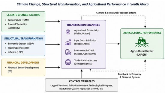
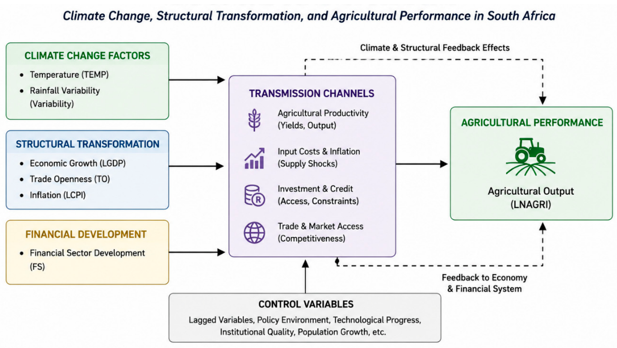
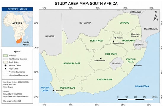
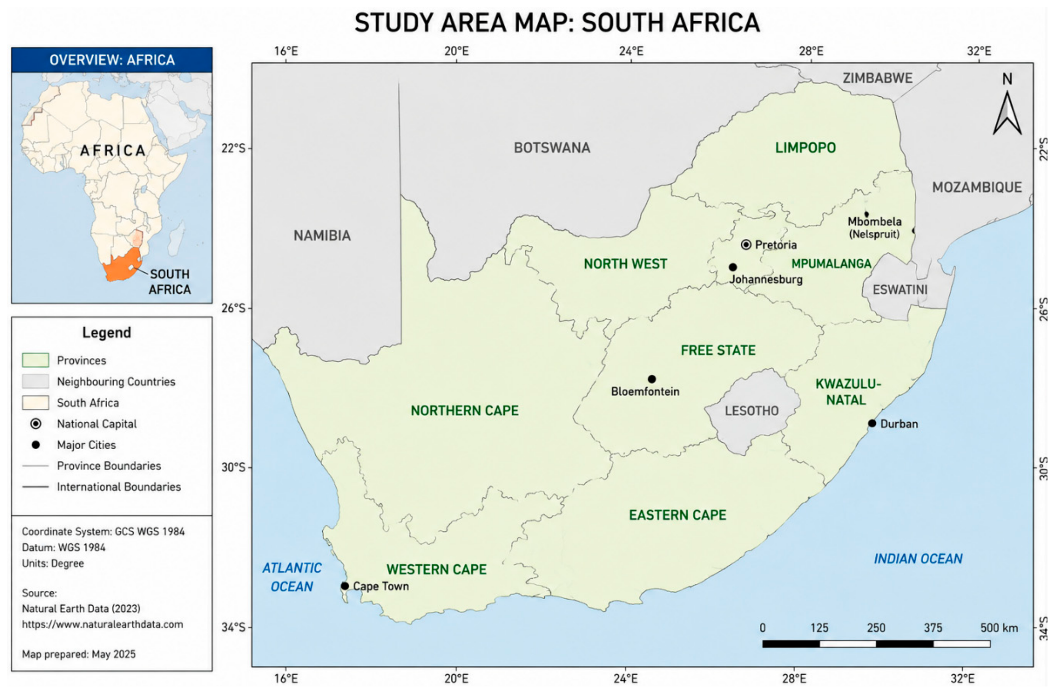
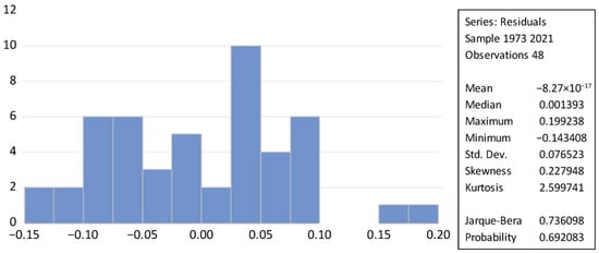
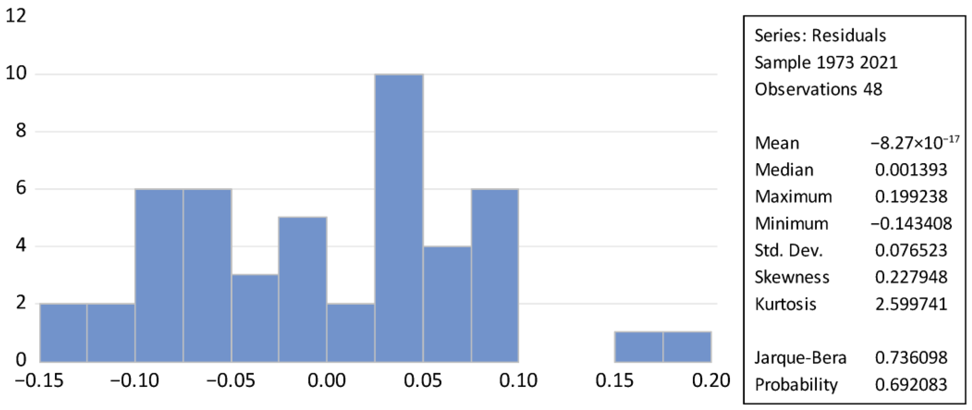
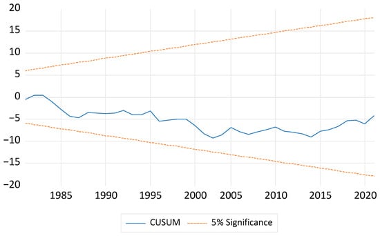
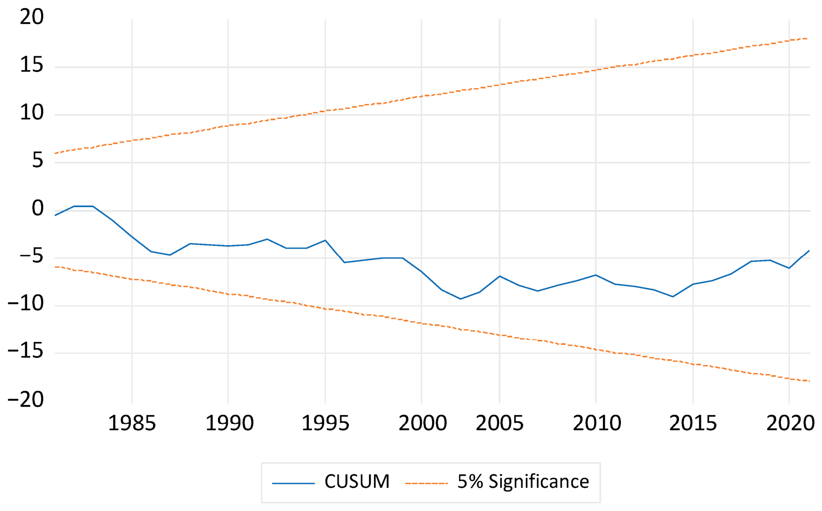

Disclaimer/Publisher’s Note: The statements, opinions and data contained in all publications are solely those of the individual author(s) and contributor(s) and not of MDPI and/or the editor(s). MDPI and/or the editor(s) disclaim responsibility for any injury to people or property resulting from any ideas, methods, instructions or products referred to in the content. |
© 2026 by the authors. Licensee MDPI, Basel, Switzerland. This article is an open access article distributed under the terms and conditions of the Creative Commons Attribution (CC BY) license.