Garden Surface Temperature Contrasts Across Urbanization Gradients: Implications for Sustainable Planning

Abstract

To inform sustainable urban and rural landscape planning, this study examines summer daytime land surface temperature (LST) contrasts at 285 garden sites across urbanization gradients in Jiangsu, China. Temperature contrast (TC) is the median within-scene difference between a 500–1000 m reference annulus and a 200 m core—positive values indicate a cooler core. Mean TC was 0.034, −0.310, and −0.588 °C in low, medium, and high urbanization classes, respectively, with a small distributional effect. Garden functional type and its interaction with urbanization did not show significant effects. A standardized model explained 56.3% of TC variation, while component regressions for core and reference LST yielded R² values of 0.736 and 0.691. Water and vegetation indicators were more strongly associated with core LST, and urbanization with reference LST. A supplementary same-scene analysis of 6 spatial definitions covered 282 sites and quantified how TC estimates changed with core and reference radii. MGWR explained 68.0% of in-sample TC variation, with the greatest fitted geographic differentiation for water probability. These findings support context-sensitive assessment of green–blue infrastructure in sustainable urban and rural landscape planning.

1. Introduction

Urbanization alters surface energy exchange by replacing vegetated and permeable land with impervious surfaces and three-dimensional built structures. Satellite observations have, therefore, identified the surface urban heat island as a persistent feature of urban development [1]. Its magnitude varies with background climate, population, city size, and urban form [2,3], while humid urban regions may experience combined heat and moisture stress [4]. These pressures make the thermal performance of landscaped open spaces an important component of sustainable landscape planning for urban heat mitigation [5,6].

Garden spaces are a specific form of planned landscape within this wider urban thermal system. Unlike a generic land-cover class, a garden is organized around an intentional combination of vegetation, tree canopy, water elements, paths, buildings, and other hard surfaces. Urban parks, country gardens, private gardens, public-affiliated gardens, and religious gardens differ in function and cultural setting, but all can provide localized thermal regulation through shading, evapotranspiration, evaporation, and altered heat storage. Systematic evidence demonstrates that urban greening can reduce local temperatures [7], while broader syntheses identify greenery as an important heat-mitigation and climate-adaptation strategy [8].

Blue and green infrastructure can provide complementary cooling through vegetation, shade, and evaporative surfaces [9,10]. Their effectiveness is nevertheless conditioned by spatial scale and threshold size [11], as well as by the design techniques used to configure green infrastructure [12]. Recent reviews have also emphasized the need for consistent cooling metrics and spatially explicit data [13,14]. Bibliometric evidence documents the rapid expansion of this field [15], while planning research increasingly connects blue–green cooling assessment with spatial optimization [16].

Most empirical evidence, however, is framed around urban parks or green spaces rather than garden spaces as a heterogeneous landscape category. Sub-meter mapping across major Chinese cities has revealed substantial variation in green-space cooling [17]. A wider comparison of 311 Chinese cities similarly showed that cooling potential changes across climate zones [18]. At the local scale, background urban heat features alter park cooling performance [19], and an urban–rural gradient has been observed for park green spaces in Shanghai [20]. Cross-climate evidence further indicates that park cooling efficiency is sensitive to both climate and area thresholds [21].

Recent studies have, therefore, begun to separate internal landscape characteristics from external urban context [22] and to quantify interactions between people-related and built-environment factors [23]. Case evidence from Hangzhou demonstrates that park cooling benefits vary among sites [24], while research on hot extremes distinguishes maximum from cumulative cooling performance [25]. Remote sensing retrieval in Shanghai confirms that park landscapes modify local thermal conditions [26]. Park size gradients [27] and pocket green spaces in high-density districts [28] provide further evidence that cooling depends on measurable spatial attributes. The thermal performance of a garden, therefore, cannot be inferred from its functional label alone—it must be evaluated from its environmental setting.

The surrounding urbanization context is particularly important when garden cooling is measured as a temperature contrast with nearby land. A garden embedded in a dense built environment may face a warmer background but may also have less space for vegetation and water. Community-level assessment in Nanjing has shown that park cooling services vary with the urban setting [29]. Research in Wuhan demonstrates that urban form helps explain spatial heterogeneity in water cooling [30]. Remote sensing studies in Beijing also reveal that the cooling effect of permanent green spaces is dynamic and scale dependent [31,32].

Evidence from 276 Chinese cities indicates that the drivers of park cooling vary across climatic and urban contexts [33], while local background climate can alter both the dominant factors and size thresholds of cooling [34]. Seasonal analysis in Nanjing confirms that these relationships are not temporally constant [35]. Peri-urban parks likewise display distinctive spatiotemporal cooling patterns and drivers [36]. Urbanization should, therefore, be treated as the context in which garden thermal performance is realized, rather than as a single direct cause.

Vegetation and water provide the most direct environmental pathways through which garden spaces can modify surface temperature. Tree canopy reduces daytime heating through shading and evapotranspiration [37,38], while vegetation amount and spatial structure influence local thermal response [39,40]. Waterbody cooling exhibits a measurable patch-size threshold [41], and thermal simulations show that coordinated blue–green planning can improve the urban thermal environment [42]. Park-focused research also demonstrates that thermal impacts can be translated into spatial optimization strategies [43].

These processes vary over time and among local landscape settings. ECOSTRESS observations reveal pronounced diurnal variation in park cooling [44], while machine learning evidence identifies nonlinear spatiotemporal relationships within blue–green systems [45]. International reviews frame blue–green solutions as an important component of climate-resilient cities [46]. Seasonal variability has been documented for parks in Nanjing [35], and random forest and SHAP analyses show that wetland-park cooling drivers also vary among sites [47]. For a province-wide garden sample, vegetation and water should, therefore, be examined as continuous characteristics of each garden-centered environment rather than assumed from garden category.

The unresolved question is how thermal differences around heterogeneous garden sites relate jointly to functional classification, surrounding development, and local land cover. Existing park studies show that area, background climate, and internal and external landscape characteristics affect measured cooling [19,21,22,27,34], but functional categories alone do not establish comparable thermal conditions across a provincial urbanization gradient. The present study addresses this question through a provincial comparison of garden-centered neighborhoods using a common observation design, complementing studies of cooling within delineated parks. It brings functional type, urbanization context, and continuous vegetation and water indicators into one assessment and examines geographic variation in their conditional associations. Its value lies in testing whether familiar functional labels and urbanization classes differentiate observed thermal conditions, and in identifying environmental associations across a broader range of garden settings. Standardized buffers define the neighborhood comparison—garden-specific attribution remains outside its scope.

Accordingly, this study evaluates 285 garden sites distributed across all 13 prefecture-level cities of Jiangsu Province. It asks three closely connected questions: (1) How does the signed garden-centered surface temperature contrast vary from low- to high-urbanization settings? (2) What associations are observed with functional garden type and vegetation and water indicators? (3) How broadly are these conditional associations estimated across the provincial sample? A multidimensional urbanization index (UI), paired same-scene Landsat temperature contrasts, global statistics, and multiscale geographically weighted regression (MGWR) address these questions. The 285-site comparison provides a provincial benchmark of observed thermal contrasts, tests the additional information provided by functional labels, and evaluates whether variable-specific spatial smoothing improves the representation of environmental associations. These results inform stratified site assessment and hypotheses for subsequent boundary-based research. For sustainable urban and rural landscape planning, the findings offer a basis for identifying garden-centered neighborhoods where local green–blue infrastructure warrants further site-specific assessment.

2. Materials and Methods

2.1. Study Area and Definition of Garden Spaces

Jiangsu Province lies in eastern China in the lower Yangtze River region. Its low-relief terrain, dense river–lake network, and climatic transition from humid subtropical conditions in the south to warmer temperate monsoon conditions toward the north create varied thermal and hydrological settings. Rapid and uneven development has also produced strong contrasts in population concentration, built form, and land development intensity between southern, central, and northern Jiangsu. This combination provides a continuous provincial gradient for examining how garden spaces perform thermally under different levels of urbanization.

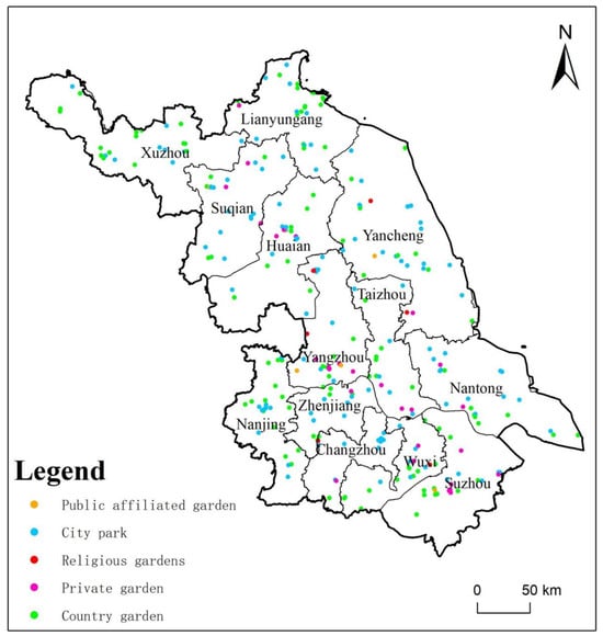
Garden-site points of interest (POIs) were obtained from the Digital Culture and Tourism query system maintained by the Jiangsu Provincial Department of Culture and Tourism (https://wlt.jiangsu.gov.cn/col/col86577/index.html, accessed on 15 December 2025). The garden-type scenic-area records were organized as a point database containing coordinates, administrative location, and functional category. This source-based POI database provided the site locations for the 2025 remote sensing assessment—the acquisition date of the site list is distinct from the observation period of the environmental variables. The analytical database comprised 285 sites across all 13 prefecture-level cities (Figure 1): 122 city (urban) parks, 118 country gardens, 32 private gardens, 7 public-affiliated gardens, and 6 religious gardens. These paired category names refer to the same functional groupings throughout the analysis. In this study, “garden space” is an operational umbrella term for these purposefully landscaped sites—it does not imply that the five categories have identical form, ownership, or design. The source-based site set supports comparisons among the recorded locations, rather than a probability sample estimate of all gardens in Jiangsu. Because consistent polygon boundaries were unavailable, standardized garden-centered neighborhoods were used to measure thermal conditions around each POI. Functional type and urbanization class are distinct classifications: “country garden” is a functional label, whereas urbanization class is assigned from the continuous neighborhood index.

Figure 1. Study area and distribution of the 285 garden spaces by functional type across the 13 prefecture-level cities of Jiangsu Province, China.

2.2. Data Sources and Preprocessing

All remotely sensed and gridded datasets were accessed and processed in Google Earth Engine (GEE), which supports large-scale cloud-based geospatial analysis [48]. The environmental analysis used 2025 as the common reference year. Summer optical and thermal observations were restricted to June–August 2025 to characterize the period of strongest vegetation activity and thermal stress. The principal data sources are summarized in Table 1.

Table 1. Data sources and their roles in the analysis.

Dataset	Reference Period	Resolution	Variables/Bands	Analytical Role
Garden POI database	15 December 2025	Point	Coordinates, garden type, administrative attributes	Sampling units
GHSL Population P2023A [49]	2025	100 m	population_count	Population density/UI
GHSL Built Surface P2023A [49]	2025	100 m	built_surface	Built-up fraction/UI
GHSL Building Volume P2023A [49]	2025	100 m	built_volume_total	Building-volume intensity/UI
Sentinel-2 SR Harmonized [50]	Jun–Aug 2025	10–20 m	B3, B4, B8, B11, SCL	NDVI, NDBI, MNDWI
Dynamic World V1 [51]	Jun–Aug 2025	10 m	trees, water, built probabilities	Tree and water context; contextual built indicator
Landsat 8/9 C2 L2 [52,53]	Jun–Aug 2025	30 m product grid	ST_B10, QA_PIXEL, QA_RADSAT	LST and paired temperature contrast (TC)
VIIRS DNB Monthly V1 [54]	Jan–Dec 2025	~464 m	avg_rad, cf_cvg	Independent UI validation

Urbanization variables were derived from the Global Human Settlement Layer (GHSL) P2023A products, which provide globally consistent population, built-up surface, and building-volume information [49]. Sentinel-2 surface reflectance (SR) provided the normalized difference vegetation index (NDVI), normalized difference built-up index (NDBI), and modified normalized difference water index (MNDWI), with the Scene Classification Layer (SCL) used for screening [50]. Dynamic World provided 10 m tree, water, and built-class probabilities [51]. Landsat 8 and Landsat 9 Collection 2 Level-2 (C2 L2) land surface temperature (LST) products were used for thermal analysis [52,53]. Monthly Visible Infrared Imaging Radiometer Suite (VIIRS) Day/Night Band (DNB) composites provided nighttime-light radiance for external comparison with the UI [54].

2.3. Garden-Centered Analytical Units

Three standardized neighborhoods were defined around each garden point. A 200 m radius core defined the local garden-centered environment for summarizing vegetation, water, and surface temperature. A 1 km neighborhood represented the surrounding urbanization context. The thermal background was defined as the annulus between 500 and 1000 m, reducing overlap with the immediate garden-centered area. These units support consistent comparison among 285 sites of different and incompletely mapped sizes, but they do not reproduce exact garden boundaries. The spatial units were defined as follows:

G_i = B₂₀₀(i),

(1)

S_i = B₁₀₀₀(i) − B₅₀₀(i),

(2)

where G_i denotes the standardized garden-centered core and S_i the surrounding thermal reference annulus. TC denotes their signed same-scene surface temperature contrast throughout the equations, tables, and figures. The two zones are fixed sampling neighborhoods rather than mapped garden footprints. A positive TC indicates that the core is cooler than its surroundings for the selected observation and location—neither sign provides a causal estimate of cooling generated by the garden.

The radii are operational sampling choices rather than empirical estimates of cooling distance. The 200 m core covers approximately 12.57 ha, while the 500–1000 m annulus represents the surrounding thermal reference environment. The intervening gap reduces overlap between measurement zones but does not exclude portions of larger gardens or adjacent green–blue spaces from the reference annulus. To examine sensitivity to spatial support, a supplementary same-scene analysis compared 150, 200, and 300 m cores with both 500–1000 and 1000–1500 m reference annuli. Within this sensitivity analysis, the 200 m core and 500–1000 m annulus served as the common reference definition.

2.4. Construction and Validation of the Urbanization Index

Urbanization was represented using four complementary dimensions: population density (POP), built-up fraction (BUILT), building-volume intensity (VOLUME), and the normalized difference built-up index (NDBI). Population density and building volume were strongly right-skewed and were, therefore, transformed as ln(X + 1). To limit sensitivity to extreme observations, each indicator was normalized using the 2nd and 98th percentiles calculated across the 285 garden neighborhoods:

X_n = (X − P₂)/(P₉₈ − P₂),   constrained to [0, 1].

(3)

The four normalized dimensions were combined using equal weights. Equal weighting was selected to maintain transparency and avoid introducing an unsupported subjective hierarchy among the urbanization components:

UI_i = (POP_n,_i + BUILT_n,_i + VOLUME_n,_i + NDBI_n,_i)/4.

(4)

Dynamic World built probability was not included in the composite index because it would duplicate built-environment information already represented by GHSL and NDBI. VIIRS nighttime lights were also excluded from the index and reserved for external validation. Annual nighttime-light radiance was calculated as the cloud-free-observation-weighted mean of the monthly VIIRS composites. The 33rd and 67th percentiles of UI divided the 285 samples into low, medium, and high urbanization classes, yielding 95 gardens in each class. For spatial visualization, the same normalized component surfaces were extended across Jiangsu and the sample-derived P33 and P67 thresholds were applied to generate province-wide UI and low–medium–high urbanization class rasters. These continuous maps were used only to characterize spatial context and did not alter the 285-site statistical classification.

2.5. Vegetation and Water Characteristics of Garden-Centered Areas

Sentinel-2 observations were screened with the Scene Classification Layer to remove invalid pixels, cloud shadow, cloud, cirrus, and snow/ice. Summer median reflectance was used to derive the normalized difference vegetation index (NDVI), NDBI, and the modified normalized difference water index (MNDWI). Within the 200 m garden-centered core, NDVI characterized overall vegetation greenness and MNDWI provided an auxiliary spectral indicator of surface water. NDVI and MNDWI were calculated as:

NDVI = (B₈ − B₄)/(B₈ + B₄),

(5)

MNDWI = (B₃ − B₁₁)/(B₃ + B₁₁).

(6)

Dynamic World images from the same summer period were averaged within each 200 m garden-centered core to obtain TreeProb and WaterProb. These are mean class probabilities and were treated as continuous indicators of tree and water likelihood, not as literal percentages of garden area [51]. Because the core may include adjacent land where exact garden boundaries are unavailable, the variables describe the environmental context centered on each garden. Table 2 summarizes the statistical variables. Province-wide NDVI, TreeProb, and WaterProb surfaces were used only to visualize the wider setting, and inference used values extracted for the 285 garden-centered cores.

Table 2. Variables used in the statistical analysis.

Variable	Definition	Spatial Scale	Role
TC	Median same scene (background LST − core LST)	200 m vs. 500–1000 m	Dependent variable
UI	Composite population–built surface–building volume–NDBI index	1 km	Main explanatory variable
NDVI	Sentinel-2 vegetation greenness	200 m	Vegetation indicator
MNDWI	Sentinel-2 modified normalized difference water index	200 m	Auxiliary water indicator
TreeProb	Mean Dynamic World tree probability	200 m	Tree indicator
WaterProb	Mean Dynamic World water probability	200 m	Water indicator
Garden type	Five functional garden categories	Site	Categorical variable
NTL	VIIRS nighttime-light radiance	1 km	Independent UI validation

2.6. Garden-Centered Surface Temperature Contrast

Landsat 8/9 Collection 2 Level-2 images acquired from June to August 2025 were filtered to scenes containing valid surface temperature products. The quality-assurance bands for pixel conditions (QA_PIXEL) and radiometric saturation (QA_RADSAT) were used for screening. Fill, cloud, cirrus, cloud-shadow, snow, and radiometrically saturated pixels were removed using QA_PIXEL and QA_RADSAT. ST_B10 was converted to degrees Celsius using the Collection 2 scale and offset [52,53]:

LST (°C) = ST_B10 × 0.00341802 + 149.0 − 273.15.

(7)

Core and background LST were calculated from the same Landsat acquisition rather than from separate seasonal mosaics. For garden i and scene t, the paired garden-centered surface temperature contrast was defined as:

TC_i,_t = LSTbackground,_i,_t − LSTcore,_i,_t.

(8)

Land surface temperature (LST) differences retain their sign. Positive values indicate that the 200 m garden-centered core was cooler than its 500–1000 m background, whereas negative values indicate a warmer core. Only scenes with valid observations in both zones were retained. The final TC value for each garden was the median of its paired scene differences:

TC_i = median(TC_i,₁, TC_i,₂, …, TC_i,_n).

(9)

Hereafter, the signed paired outcome is denoted TC (temperature contrast), in degrees Celsius—its positive/negative sign concerns the sampled core relative to the annulus rather than a causal garden cooling effect.

This definition is intentionally based on the median of paired differences rather than the difference between independently calculated seasonal medians. All 285 gardens contained at least 3 valid paired observations—the valid-scene count ranged from 3 to 24 and averaged 9.18 scenes per garden. A province-wide summer median LST raster was also produced to visualize the regional thermal background. This contextual raster was not used to replace the same-scene paired TC metric used in the statistical analyses.

2.7. Statistical Analysis of Garden-Centered Temperature Contrasts

The analysis followed the three research questions. First, TC was compared among low, medium, and high urbanization classes using one-way analysis of variance (ANOVA) and the Kruskal–Wallis test. The latter was the principal comparison because the reported distributions showed unequal spread and outlying values. It compares ranks across groups without requiring normally distributed errors and is interpreted here as a distributional comparison, not solely as a test of medians: a location-shift interpretation requires similarly shaped distributions. One-way ANOVA is retained as a complementary comparison of means—the two tests need not agree because they address different features of the distributions. Mann–Whitney U tests with Holm correction were used for pairwise contrasts. Both approaches assume independent observations. Spatial diagnostics help assess this assumption but do not prove independence, particularly where buffers overlap. The reported ε² is a rank-based effect-size estimate, not the proportion of raw temperature variance explained.

Second, a factorial linear model included garden type, urbanization class, and their interaction. Type III tests evaluate each term conditional on the other included terms in this unbalanced design. “Robust” refers to covariance-based inference allowing unequal error variances—it does not mean that sparse categories, omitted area, or spatial dependence have been corrected. The model assumes an adequately specified conditional mean and estimable categorical contrasts, and the small type-by-class cells limit precision. Pearson correlations describe linear associations, whereas Spearman correlations describe monotonic rank associations and are less sensitive to extreme magnitudes. Reporting both reveals whether an association is sensitive to linearity and influential values. A standardized ordinary least squares (OLS) regression used UI, NDVI, TreeProb, and WaterProb with heteroscedasticity-consistent type 3 (HC3) standard errors and variance inflation factor (VIF) diagnostics. HC3 addresses unequal residual variances, not spatially correlated errors. Garden type was added in a secondary model to assess additional in-sample information. All coefficients are conditional observational associations.

As a measurement construction diagnostic, the same standardized HC3-OLS specification (UI, NDVI, TreeProb, and WaterProb; n = 285) was additionally fitted to the separately stored scene-matched core and reference LST medians. Each outcome was standardized independently. The component models are not an algebraic coefficient decomposition of TC: TC is the median of within-scene differences, which generally differs from the difference between separately aggregated scene medians. They test which temperature zone shows the stronger conditional association with each predictor.

A supplementary same-scene radius sensitivity analysis was conducted in Google Earth Engine using 2025 summer Landsat 8/9 observations and the same thermal-band scaling and pixel-quality screening. Six spatial definitions paired 150, 200, and 300 m cores with 500–1000 and 1000–1500 m reference annuli. For each valid acquisition, the median surface temperature was calculated separately for each zone. TC was then defined as the within-scene reference-minus-core difference and summarized by its median across acquisitions. A scene was retained only when valid pixels were present in all five zones, thereby keeping the observation set identical among the six definitions at each site. Requiring at least 3 common valid scenes retained 282 gardens (94 in each urbanization class). Radius effects were summarized as within-site differences relative to the 200 m core and 500–1000 m annulus in this same-scene sensitivity dataset. These paired differences quantify the influence of sampling radii on measured TC, without assigning a causal thermal effect to garden boundaries.

2.8. Spatial Modeling of Conditional Associations

Spatial analysis combined global and local autocorrelation with geographically weighted regression. Garden coordinates were projected to World Geodetic System 1984/Universal Transverse Mercator Zone 50N (WGS 84/UTM Zone 50N; EPSG:32650) for distance-based modeling. Global Moran’s I was calculated for TC and model residuals using an 8-nearest-neighbor spatial weights matrix and 999 permutations for inference [55]. For TC, k = 4 and k = 12 were also examined as sensitivity tests. Positive Moran’s I indicates similarity among neighboring values, whereas negative values indicate spatial dissimilarity, relative to the randomization reference. Permutation inference compares the observed statistic with statistics obtained by reallocating values among the fixed site locations. A non-significant result means that this test did not detect dependence under the specified weights. Local Moran’s I identified high–high, low–low, high–low, and low–high associations [56]. Its unadjusted site-level p-values are exploratory because testing many locations can produce chance flags.

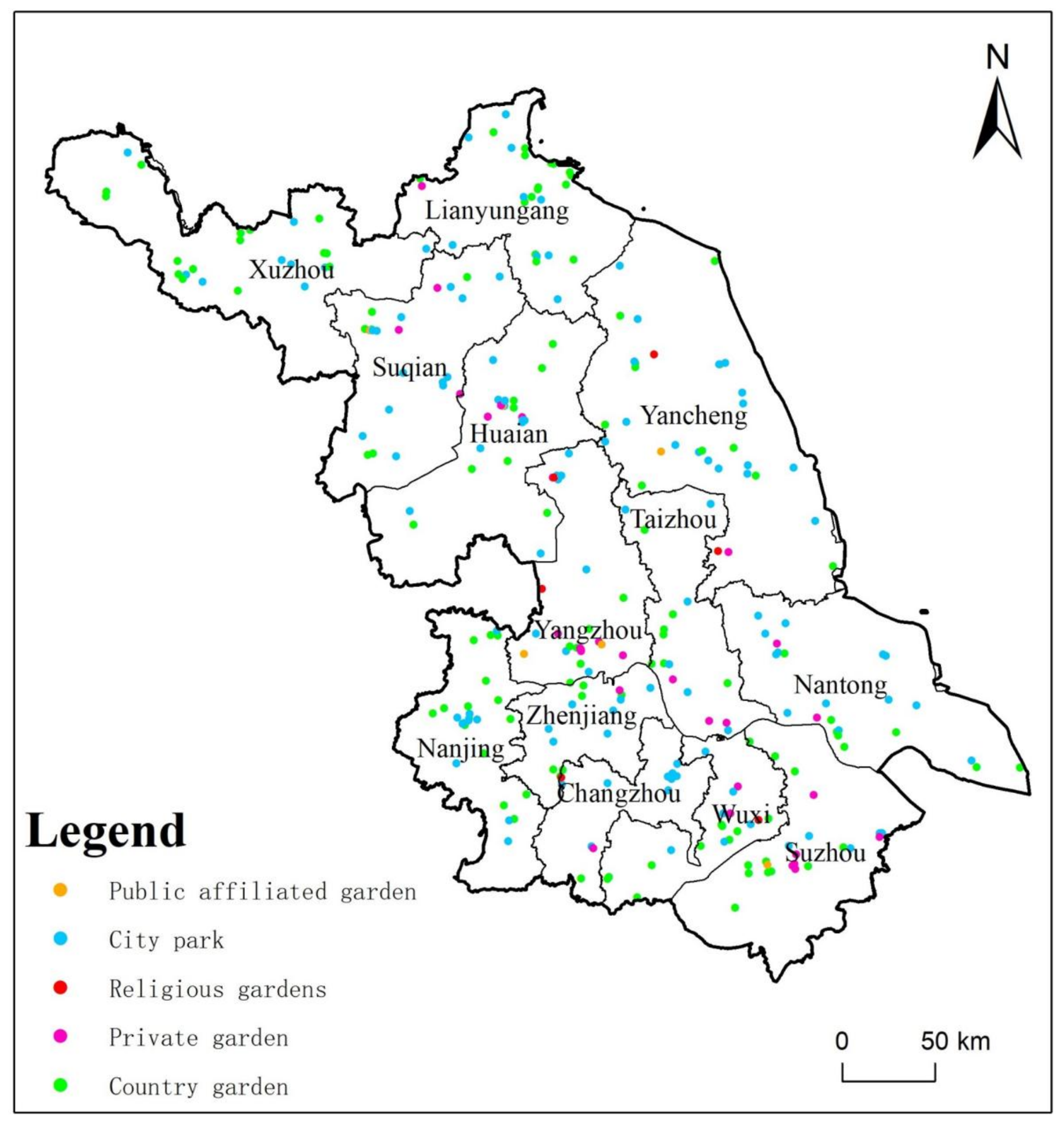
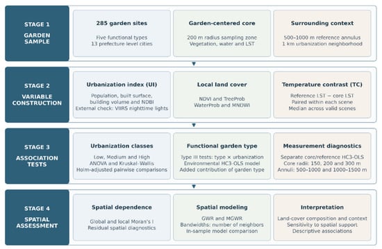
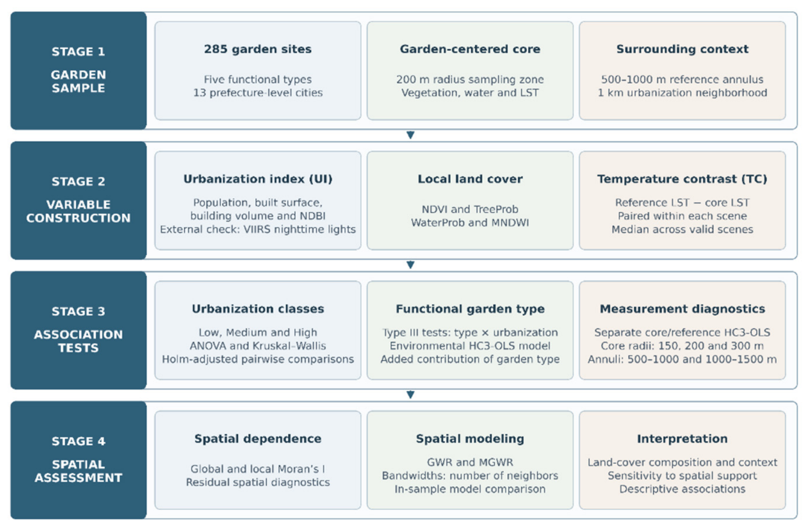
Because spatial dependence remained in OLS residuals, geographically weighted regression (GWR) and MGWR were calibrated using the same four continuous predictors. GWR permits local coefficients with a single bandwidth [57], whereas MGWR estimates variable-specific smoothing bandwidths [58,59]. An adaptive bi-square kernel and bandwidth optimization based on the corrected Akaike information criterion (AICc) accommodated the uneven site distribution. An adaptive bandwidth is a neighbor count, not a fixed distance in meters—the corresponding geographic extent varies with sample density. Bandwidths describe coefficient estimation in this fitted model, not the physical reach of cooling or a demonstrated causal mechanism. Model performance was compared using R², adjusted R², AICc, and residual Moran’s I. These are in-sample diagnostics, not independent predictive validation. The complete workflow is summarized in Figure 2.

Figure 2. Analytical workflow for signed garden-centered temperature contrast (TC), core/reference LST component models, and same-scene spatial-support sensitivity. Local smoothing in MGWR refers to the fitted model, not a physical cooling distance.

3. Results

3.1. Urbanization Context and Index Validation

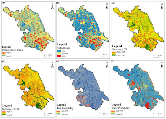
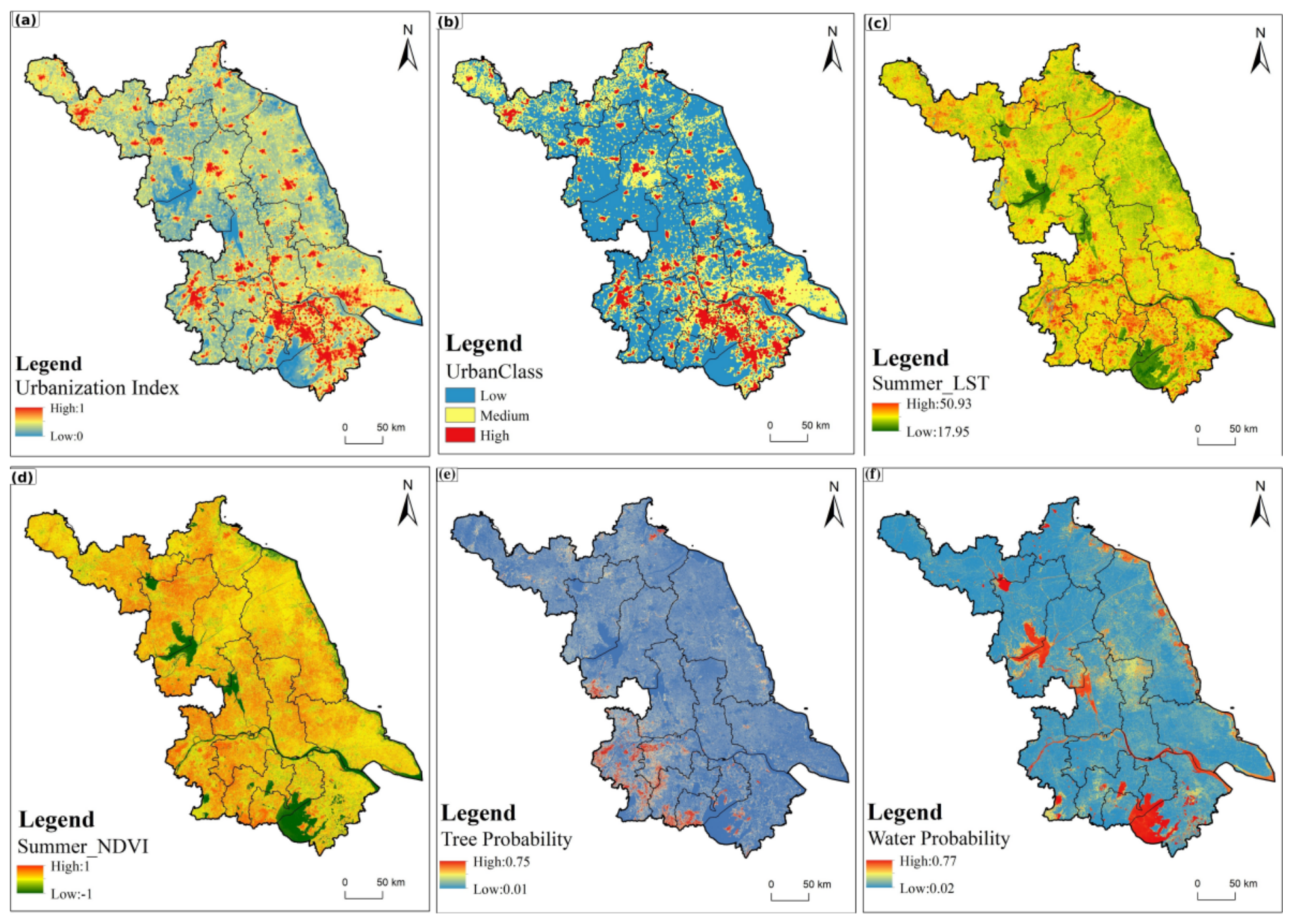
The 285 garden sites were embedded in markedly different urbanization settings (Figure 3a,b). High UI values were concentrated in southern Jiangsu and around major prefecture-level urban centers and development corridors, while lower values occupied broader peri-urban and rural areas. Applying the sample-derived P33 and P67 thresholds produced a spatially coherent low–medium–high gradient. This pattern establishes the built-environment context against which the garden-centered temperature contrasts were compared.

Figure 3. Spatial patterns of (a) the urbanization index, (b) low, medium, and high urbanization classes, (c) summer land surface temperature, (d) summer NDVI, (e) Dynamic World tree probability, and (f) Dynamic World water probability across Jiangsu Province in 2025.

The same garden network also occupied diverse thermal, vegetation, tree, and water settings (Figure 3c–f). Warmer LST patches generally corresponded to developed land, while major lakes, river corridors, and some less intensively developed landscapes were cooler. NDVI represented overall vegetation greenness, TreeProb isolated tree-class likelihood, and WaterProb highlighted major lakes and river corridors. These maps do not describe the exact design of individual gardens, but they demonstrate that gardens across Jiangsu are situated in substantially different local environments that may influence the measured core-to-annulus contrasts.

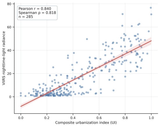
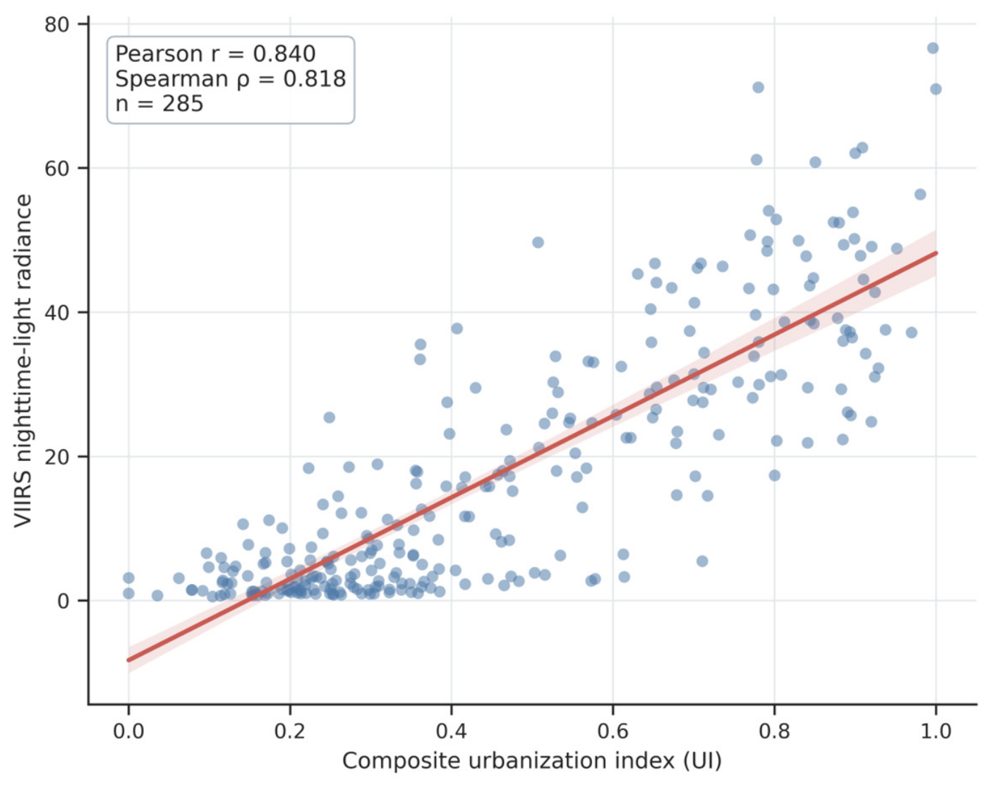
The mapped UI pattern was consistent with the spatial concentration of developed areas shown in Figure 3a,b. At the garden-neighborhood scale, the composite UI was also closely associated with independent VIIRS nighttime-light radiance. Pearson’s correlation was r = 0.840 (p < 0.001), while Spearman’s rank correlation was ρ = 0.818 (p < 0.001). This agreement indicates that the multidimensional index captured meaningful differences in urban activity intensity even though nighttime lights were not used in index construction. The independent validation relationship is shown in Figure 4.

Figure 4. External validation of the composite urbanization index against VIIRS nighttime-light radiance. The line and shaded band show the fitted linear relationship and its 95% confidence interval.

3.2. Temperature Contrasts Across Urbanization Classes and Garden Types

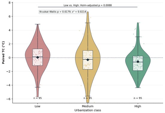
Garden-centered TC varied widely among sites, and both mean and median values shifted from slightly positive in the low class to negative in the medium and high classes (Figure 5). Mean values were 0.034 °C, −0.310 °C, and −0.588 °C, respectively, and the corresponding medians were 0.131 °C, −0.249 °C, and −0.632 °C. Thus, the group-level contrast reversed sign: cores in the medium and high groups were warmer than their reference annuli on average. This statement concerns class summaries and does not mean that every site in these groups was warmer. Summary statistics are reported in Table 3.

Figure 5. Distribution of signed garden-centered surface temperature contrast across low, medium, and high urbanization classes. Violin and box plots are overlaid with individual sites and group means, and the significant Holm-adjusted low–high comparison is indicated. Negative values denote a warmer core.

Table 3. Signed garden-centered surface temperature contrast across urbanization classes.

Urbanization Class	N	Mean (°C)	Median (°C)	SD (°C)
Low	95	0.034	0.131	1.955
Medium	95	−0.310	−0.249	2.492
High	95	−0.588	−0.632	1.778

Note: Kruskal–Wallis H = 8.045, p = 0.0179; ε² = 0.0214.

The ANOVA did not identify a significant difference in group means (F = 2.098, p = 0.1247), whereas the Kruskal–Wallis test detected a difference in the distributions (H = 8.045, p = 0.0179). The rank-based effect size was small (ε² = 0.0214), consistent with substantial within-class heterogeneity. It should not be read as 2.1% of raw temperature variance explained. Holm-adjusted pairwise tests identified a low–high contrast (pHolm = 0.0088), while low–medium and medium–high contrasts were not significant (Figure 5).

The robust factorial model did not detect a significant garden-type main effect (p = 0.278), conditional urbanization class effect (p = 0.908), or garden type × urbanization interaction (p = 0.365)—the reported interaction partial η² was 0.032 (Table 4). These tests provide no statistical support for differentiating the observed contrasts by functional type under this specification. They do not establish equivalence—the unbalanced type-by-class distribution and omitted garden area limit the precision and interpretation of type comparisons.

Table 4. Robust Type III analysis of garden type and urbanization gradient.

Effect	df	F	p	Partial η2
Garden type	4	1.279	0.278	0.019
Urbanization class	2	0.096	0.908	0.001
Garden type × Urbanization	8	1.098	0.365	0.032

Note: The factorial effects are conditional on the other model terms. Rare garden categories contain small cell counts and should be interpreted cautiously.

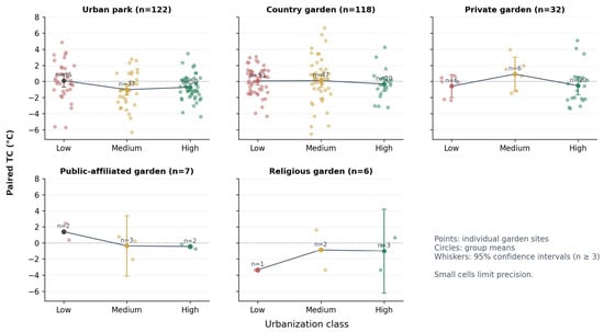
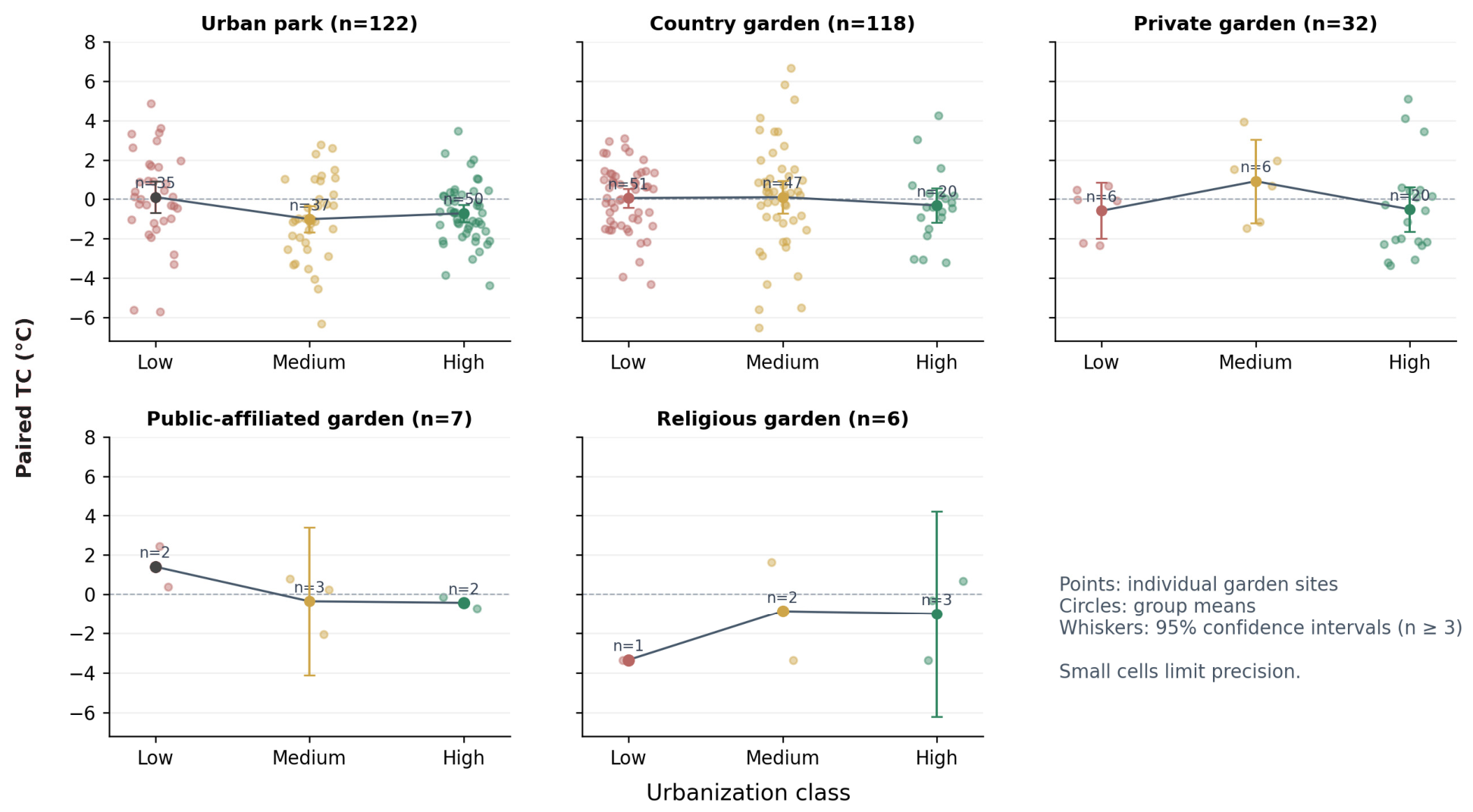
The type-specific trajectories differed numerically, but the factorial tests did not establish corresponding differences (Figure 6). Urban parks and country gardens supplied most observations, and public-affiliated gardens (n = 7) and religious gardens (n = 6) had type-by-class cells as small as one or two. The cross-tabulation in Table 5 shows that country gardens occurred in all 3 UI classes, with 51, 47, and 20 sites in the low, medium, and high classes. Functional type is, therefore, associated with, but does not determine, the statistical urbanization class. Unknown differences in garden area and the sparse cells remain potential sources of confounding and low precision.

Figure 6. Functional garden type × urbanization class patterns in paired temperature contrast (TC). Points represent individual gardens, and circles and whiskers indicate group means and 95% confidence intervals (shown only where n ≥ 3). Cell sample sizes are labeled.

Table 5. Cross-tabulation of garden functional type and urbanization class in the 285-site analytical dataset.

Garden Type	Low	Medium	High	Total
Urban park	35	37	50	122
Country garden	51	47	20	118
Private garden	6	6	20	32
Public-affiliated garden	2	3	2	7
Religious garden	1	2	3	6
Total	95	95	95	285

3.3. Bivariate and Conditional Environmental Associations

Garden-centered TC showed contrasting associations with urbanization, vegetation, and water variables (Table 6). UI had a weak negative Pearson association (r = −0.111, p = 0.060) and a negative Spearman association (ρ = −0.173, p = 0.003). NDVI, the normalized difference vegetation index, was weakly positive in Pearson analysis (r = 0.110, p = 0.064) but more positive in rank form (ρ = 0.277, p < 0.001). TreeProb was positive in both analyses (Pearson r = 0.300; Spearman ρ = 0.331; both p < 0.001). WaterProb had the largest Pearson association (r = 0.454, p < 0.001), whereas MNDWI showed a less consistent pattern. These are associations with the buffer contrast and do not distinguish internal garden land cover from adjacent surfaces.

Table 6. Bivariate associations between TC and major environmental variables.

Variable	Pearson r	p	Spearman ρ	p
UI	−0.111	0.060	−0.173	0.003
NDVI	0.110	0.064	0.277	<0.001
TreeProb	0.300	<0.001	0.331	<0.001
WaterProb	0.454	<0.001	0.274	<0.001
MNDWI	0.159	0.007	−0.096	0.105

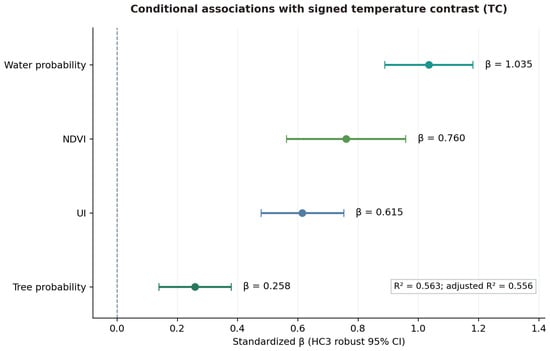
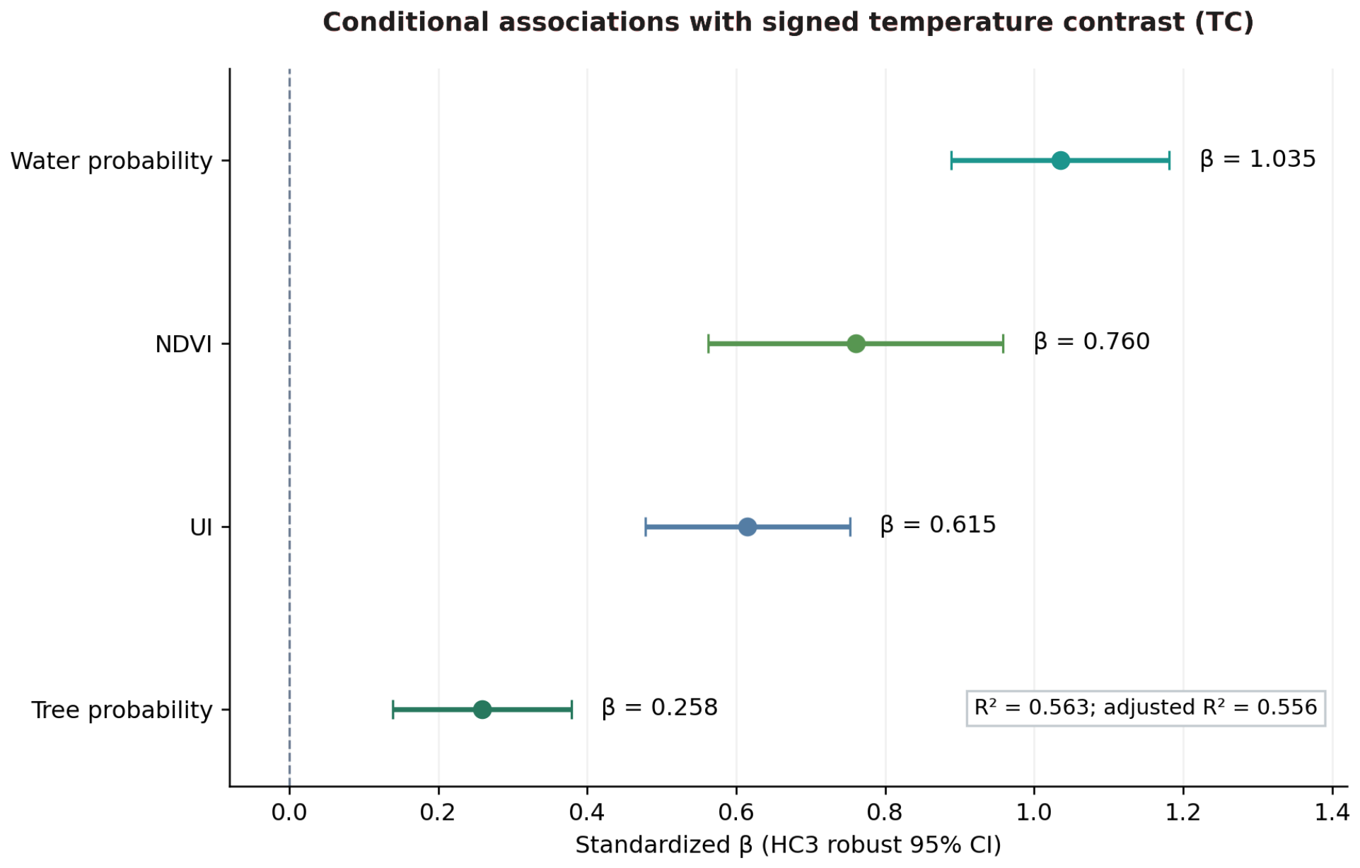
The standardized global regression explained 56.3% of in-sample variation in garden-centered TC (R² = 0.563; adjusted R² = 0.556). WaterProb had the largest standardized conditional coefficient (β = 1.035), followed by NDVI (β = 0.760), UI (β = 0.615), and TreeProb (β = 0.258)—all reported HC3 p-values were < 0.001. VIFs ranged from 2.19 to 4.51, documenting the degree of predictor correlation relevant to interpreting the conditional coefficients (Table 7).

Table 7. Standardized global regression coefficients and multicollinearity diagnostics.

Predictor	Standardized β	HC3 SE	p	VIF
UI	0.615	0.070	<0.001	2.19
NDVI	0.760	0.101	<0.001	4.51
TreeProb	0.258	0.061	<0.001	2.51
WaterProb	1.035	0.075	<0.001	2.41

UI changed from a weakly negative bivariate association to a positive conditional coefficient. Partial correlations were positive for UI (0.532), NDVI (0.476), TreeProb (0.240), and WaterProb (0.710), all with reported p < 0.001. The reversal is consistent with a suppression pattern but does not establish a separate beneficial urbanization pathway. Adding garden type increased R² from 0.563 to 0.564 and did not improve model fit (p = 0.897). This indicates little additional in-sample information from the recorded labels under this specification, rather than proof that type has no thermal relevance (Figure 7).

Figure 7. Standardized conditional coefficients and HC3 robust 95% confidence intervals for the global model of garden-centered surface temperature contrast. Coefficients describe associations under the fitted specification, not intervention effects.

The model evaluates how the observed contrast relates to land-cover composition in the core and development context in the wider neighborhood. Because the predictors share spatial support with the temperature measurements, the fitted associations can include the temperature signatures of the surfaces represented in each zone. We, therefore, interpret R² = 0.563 as an in-sample summary of associations with the defined neighborhood contrast, rather than the proportion of variation attributable to independent garden cooling processes. UI, NDVI, TreeProb, and WaterProb are derived from settlement, reflectance, and land-cover information without using LST. Comparison of bivariate and conditional associations, VIFs, and residual spatial diagnostics helps characterize the fitted relationships within this measurement design. A standardized coefficient above one is possible with correlated predictors—coefficient magnitude is not a ranking of intervention benefits.

3.4. Core/Reference Component Models and Same-Scene Spatial-Support Sensitivity

The four-predictor paired TC regression yielded R² = 0.563 (adjusted R² = 0.556). Applying the same standardized predictors to the separately stored core- and reference-zone LST medians yielded R² = 0.736 and R² = 0.691, respectively (Table 8). The core-zone coefficients for NDVI (β = −0.263, p < 0.001), TreeProb (β = −0.244, p < 0.001), and WaterProb (β = −0.578, p < 0.001) were negative. In contrast, reference-zone WaterProb was weak (β = −0.096, p = 0.163) and reference-zone NDVI was not significant (β = 0.123, p = 0.094). UI was positively associated with both zones, but its standardized association was stronger for reference LST (β = 0.791, p < 0.001) than for core LST (β = 0.352, p < 0.001). The reference-zone TreeProb association was smaller (β = −0.123, p = 0.016). These patterns indicate that the contrast-model associations partly reflect where vegetated, water, and developed surfaces fall within the measurement zones—they do not independently identify garden-mediated cooling.

Table 8. Standardized HC3-OLS component diagnostic models using identical predictors and the same 285 sites.

Response	R2	UI β	NDVI β	TreeProb β	WaterProb β
Paired TC	0.563	+0.615 ***	+0.760 ***	+0.258 ***	+1.035 ***
Core LST median	0.736	+0.352 ***	−0.263 ***	−0.244 ***	−0.578 ***
Reference LST median	0.691	+0.791 ***	+0.123 n.s.	−0.123 *	−0.096 n.s.

Note: Standardization uses each response’s own standard deviation. Entries are standardized β with HC3-robust tests. * p < 0.05; *** p < 0.001; n.s. p ≥ 0.05. The paired TC response is a median of within-scene differences, not a difference of seasonal component medians.

In the same-scene radius sensitivity analysis, 282 gardens had valid observations under all 6 core/annulus definitions (Table 9). Relative to the 200 m core and 500–1000 m annulus within that analysis, the 150 m and 300 m cores produced group-specific mean changes in TC. Extending the reference annulus to 1000–1500 m also altered the estimates. For example, holding the 500–1000 m annulus fixed, expanding the core to 300 m changed mean TC by +0.284 °C in the low group, +0.142 °C in the medium group, and −0.366 °C in the high group. Across the 282 sites, 222 retained the same individual TC sign under all 6 definitions, whereas 60 changed sign at least once. These results quantify the influence of spatial support on measured temperature contrasts and reinforce the need to distinguish a signed surface temperature contrast from a physical cooling-distance estimate.

Table 9. Same-scene radius sensitivity by urbanization class (n = 282). Entries show changes in mean site-level TC (°C) relative to the 200 m core/500–1000 m reference annulus within the same set of valid acquisitions.

Core/Reference Annulus	Low ΔTC	Medium ΔTC	High ΔTC
150 m/500–1000 m	−0.219	−0.084	+0.184
200 m/500–1000 m	0.000	0.000	0.000
300 m/500–1000 m	+0.284	+0.142	−0.366
150 m/1000–1500 m	−0.131	−0.202	−0.162
200 m/1000–1500 m	+0.065	−0.110	−0.349
300 m/1000–1500 m	+0.377	+0.040	−0.706

Note: All six definitions use the same valid Landsat acquisitions at each site (94 gardens per urbanization class). ΔTC is computed first for each site against the common 200 m/500–1000 m reference definition and then averaged by class. Zero values in the reference row arise by construction. These are radius-related changes within the matched sensitivity analysis, not absolute class-level TC means.

Table 10 provides the absolute class-level core and reference LST, together with signed TC, for all six spatial definitions. Mean core and reference LST increased from low to high urbanization across the tested definitions. Within the 282-site common-scene analysis, mean TC remained negative for low and medium and positive for high under all six definitions, while its magnitude varied with the selected radii.

Table 10. Class-level mean core LST, reference annulus LST, and signed paired TC under six same-scene spatial definitions (n = 282; 94 sites per urbanization class).

Core/Reference Annulus	Urbanization Class	Core LST (°C)	Reference LST (°C)	Mean TC (°C)
150 m/500–1000 m	Low	38.973	37.711	−1.438
150 m/500–1000 m	Medium	40.436	40.076	−0.413
150 m/500–1000 m	High	42.819	44.674	+1.851
200 m/500–1000 m	Low	38.801	37.711	−1.218
200 m/500–1000 m	Medium	40.354	40.076	−0.329
200 m/500–1000 m	High	43.037	44.674	+1.667
300 m/500–1000 m	Low	38.547	37.711	−0.932
300 m/500–1000 m	Medium	40.259	40.076	−0.187
300 m/500–1000 m	High	43.426	44.674	+1.301
150 m/1000–1500 m	Low	38.973	37.905	−1.351
150 m/1000–1500 m	Medium	40.436	39.910	−0.530
150 m/1000–1500 m	High	42.819	44.329	+1.505
200 m/1000–1500 m	Low	38.801	37.905	−1.154
200 m/1000–1500 m	Medium	40.354	39.910	−0.439
200 m/1000–1500 m	High	43.037	44.329	+1.317
300 m/1000–1500 m	Low	38.547	37.905	−0.839
300 m/1000–1500 m	Medium	40.259	39.910	−0.289
300 m/1000–1500 m	High	43.426	44.329	+0.961

Note: Entries are means across sites within the 282-site common-scene sensitivity sample. For each site and spatial definition, core and reference LST are calculated as separate medians across the same valid acquisitions. TC is the median of within-scene reference-minus-core differences.

It should be noted that the primary analysis (Table 3) and the spatial sensitivity analysis (Table 9 and Table 10) adopted different scene-selection criteria to address their respective analytical objectives. In the primary analysis, Landsat acquisitions were retained when valid LST observations were available in both the predefined 200 m core and 500–1000 m reference annulus, allowing all eligible observations to contribute to the site-level TC estimates for 285 gardens (95 per urbanization class). In contrast, the sensitivity analysis required valid observations simultaneously across all 3 core radii (150, 200, and 300 m) and both reference annuli (500–1000 and 1000–1500 m), retaining 282 gardens (94 per class) with at least 3 common valid acquisitions. This stricter criterion ensured that all six spatial definitions were evaluated using identical Landsat acquisitions at each site, thereby avoiding confounding between changes in sampling radii and differences in observation dates. Accordingly, Table 9 reports changes in TC relative to the primary spatial definition within this matched observation set, while Table 10 presents the corresponding absolute core and reference LST values and signed TC means. Although both analyses employed identical LST processing procedures and TC calculations, differences in eligible acquisitions resulted in different analytical observation sets and, consequently, different class-level means even under the same spatial definition. These differences do not alter the reported findings of the primary analysis.

3.5. Spatial Diagnostics and Model Estimation Scales

Global Moran’s I did not detect province-wide clustering of garden-centered TC: I = −0.047 (p = 0.223) for k = 4, −0.019 (p = 0.578) for k = 8, and −0.009 (p = 0.782) for k = 12. Local Moran analysis at k = 8 flagged 12 sites using unadjusted p < 0.05, while 273 sites were not significant. Because 285 locations were tested without multiplicity correction, these local flags are exploratory and do not establish confirmed thermal clusters.

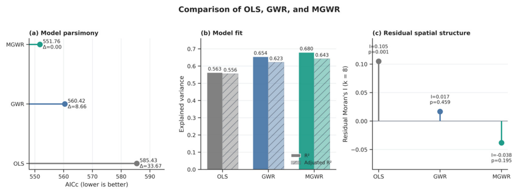
In contrast, global model residuals were positively autocorrelated (Moran’s I = 0.105, p = 0.001 for k = 8). This indicates spatial structure not captured by the global specification. Spatially varying coefficients are one possible representation of that structure, but omitted spatial covariates, overlapping analytical units, and model misspecification are also possible explanations. The residual diagnostic alone does not prove that the underlying effects vary geographically.

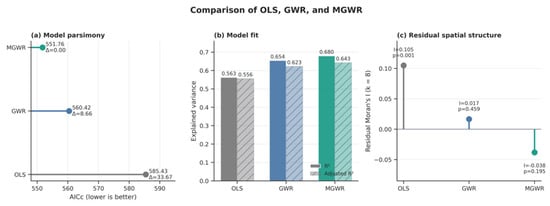
Both spatial models improved in-sample fit relative to OLS, and MGWR had the lowest AICc among the fitted models. OLS produced R² = 0.563, adjusted R² = 0.556, and AICc = 585.43. GWR increased R² to 0.654 and reduced AICc to 560.42. MGWR increased R² to 0.680 and adjusted R² to 0.643, with AICc = 551.76 (Table 11).

Table 11. Comparison of global and spatial regression models.

Model	R2	Adjusted R2	AICc	Residual Moran’s I
OLS	0.563	0.556	585.43	0.105 (p = 0.001)
GWR	0.654	0.623	560.42	0.017 (p = 0.459)
MGWR	0.680	0.643	551.76	−0.038 (p = 0.195)

Note: Lower AICc indicates better parsimony-adjusted in-sample fit. Residual Moran’s I was not significant for MGWR under the specified k = 8 test—this does not prove absence of all spatial dependence.

The ΔAICc between OLS and MGWR was 33.67, and the difference between GWR and MGWR was 8.66. Residual Moran’s I was 0.017 (p = 0.459) for GWR and −0.038 (p = 0.195) for MGWR. The tests, therefore, did not detect residual dependence for either spatial model at k = 8 (Figure 8). Together with the AICc comparison, these diagnostics support MGWR as the best-fitting representation among the models examined, while remaining conditional on the neighborhood definition and included predictors.

Figure 8. Comparison of OLS, GWR, and MGWR in terms of (a) corrected Akaike information criterion, (b) explained variance, and (c) residual spatial autocorrelation.

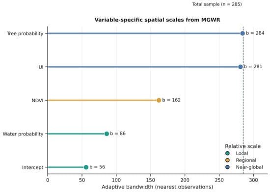
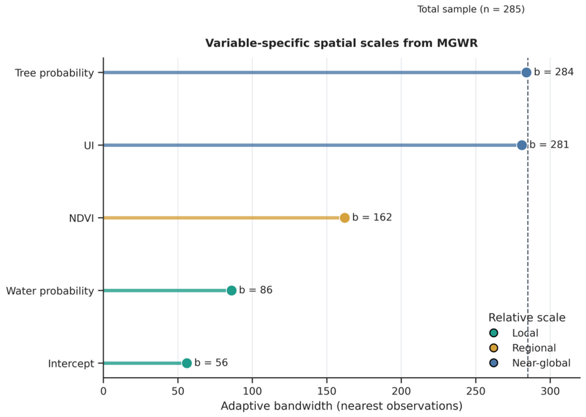
MGWR selected adaptive bandwidths of 56 for the intercept, 281 for UI, 162 for NDVI, 284 for TreeProb, and 86 for WaterProb. Relative to n = 285, UI and TreeProb were estimated with near-global smoothing, NDVI with an intermediate bandwidth, and WaterProb with the smallest predictor bandwidth (Table 12). UI coefficients ranged from 0.630 to 0.693 (range 0.063), and TreeProb coefficients from 0.298 to 0.353 (range 0.055). Their limited variation under this fit should not be interpreted as independent evidence of spatially homogeneous effects.

Table 12. MGWR variable-specific bandwidths and standardized local coefficient distributions.

Variable	Bandwidth	Mean Coefficient	Minimum	Maximum
Intercept	56	0.004	−0.547	0.391
UI	281	0.670	0.630	0.693
NDVI	162	0.793	0.612	0.930
TreeProb	284	0.335	0.298	0.353
WaterProb	86	1.099	0.848	1.397

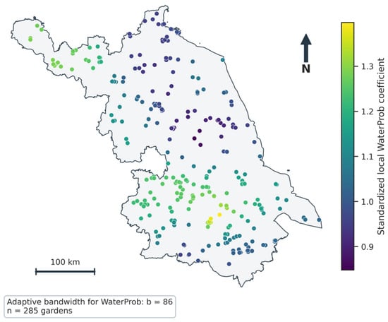
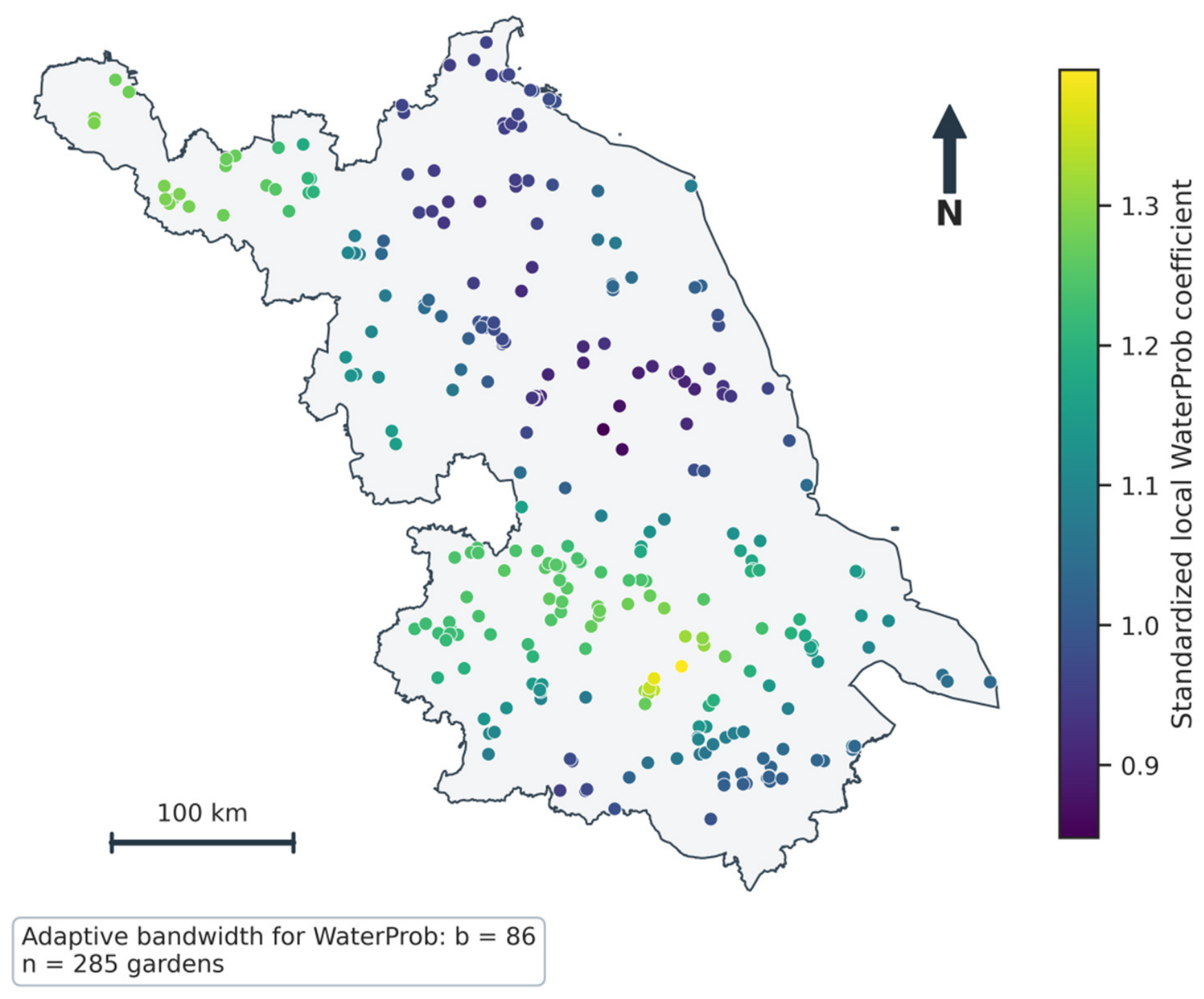
Figure 9 summarizes the selected bandwidths. WaterProb coefficients ranged from 0.848 to 1.397 (range 0.549), the widest predictor range, and NDVI coefficients ranged from 0.612 to 0.930 (range 0.318). The intercept also varied, from −0.547 to 0.391. Water, therefore, showed the clearest fitted geographic variation among the predictors, while NDVI retained an intermediate pattern. These summaries do not substitute for formal tests of coefficient non-stationarity or bandwidth uncertainty. Figure 10 maps WaterProb coefficients at the observed locations without interpolation into unsampled areas.

Figure 9. Variable-specific adaptive bandwidths estimated by MGWR. Colors indicate smaller, intermediate, and near-global neighbor counts relative to n = 285, not physical cooling distances or validated intervention scales.

Figure 10. Spatial distribution of standardized local WaterProb coefficients estimated by MGWR at the 285 garden locations within the supplied Jiangsu Province boundary.

4. Discussion

4.1. Urbanization and the Signed Temperature Contrast

The first finding is a small distributional difference in signed temperature contrasts across urbanization classes. Class means changed from approximately zero in the low group to negative in the medium and high groups, indicating warmer cores on average in the latter groups. Only the low–high pairwise comparison was significant, and within-class variability was large. Park studies in Shanghai and peri-urban China [20,36] motivate urban–rural comparisons, but their cooling metrics and site boundaries need not match the fixed-buffer outcome here. Cross-city and background-climate research [18,19], together with area-efficiency evidence [21,24], cautions against attributing this pattern to urbanization alone. Garden size was not controlled, so size differences across classes cannot be excluded. Within this scope, the result shows that the broad urbanization classes offer limited differentiation of observed thermal contrasts and cannot replace assessment of local environmental conditions.

The positive conditional UI coefficient addresses a different comparison from the class-level summaries: sites with similar core vegetation and water indicators but different wider development contexts. UI is measured over the 1 km neighborhood, which includes the reference annulus, whereas vegetation and water are summarized in the core. This alignment links the conditional coefficients to the composition of both measurement zones and limits separation of garden-mediated cooling from the temperature signatures of nearby surfaces. The coefficients consequently describe associations with the fixed-support neighborhood contrast. The distinction between internal and external park drivers in earlier studies [19,22,23] helps frame these contextual relationships, although the present design does not identify separate causal pathways.

The UI sign reversal can be described as suppression in the fitted covariance structure, but it cannot validate the proposed background-heat mechanism or quantify a benefit from urbanization. Same-scene differencing strengthens temporal comparability by comparing the two zones within each acquisition—it does not supply an untreated counterfactual. The study consequently contributes evidence on the joint contextual associations of the observed contrast. Reporting both class comparisons and conditional coefficients shows why a simple urbanization gradient is insufficient to describe that relationship.

4.2. Functional Type and Environmental Associations

The factorial model detected no significant type effect, and adding functional garden type to the environmental regression supplied little additional in-sample information under the present specification. The cross-tabulation shows uneven type distributions along the gradient, and the rare categories have very small cells. Non-significance consequently cannot establish equivalence, nor can it rule out relationships between function, area, design, and thermal conditions. Continuous NDVI, TreeProb, and WaterProb indicators describe the measured environments directly and show stronger associations with the observed contrast than the recorded labels under this specification. Their interpretation concerns land-cover composition in the core and does not isolate each garden’s thermal contribution.

WaterProb had the strongest Pearson association and the largest standardized conditional coefficient. TreeProb was also positively associated with the contrast. Canopy shading and evapotranspiration are established thermal processes [37,38], while water cooling depends on patch size [41] and surrounding urban form [30]. These studies support plausible interpretations, not direct validation by this dataset. Water within the core is itself a surface with a distinct temperature signature, so its association can arise from the construction of the outcome as well as from thermal exchange with nearby land. The coefficient β = 1.035 is a conditional standardized estimate—values greater than one are possible with correlated predictors and should not be treated as a ranking of causal intervention effectiveness.

For the Introduction’s question about functional labels, the useful result is the limited additional information supplied by the recorded categories once environmental indicators are included: R² increased from 0.563 to 0.564 (p = 0.897). This supports using continuous environmental measurements alongside functional classification when assessing the sampled neighborhoods. It does not establish thermal equivalence across garden types, especially the rare categories. Boundary-based area controls and more observations in sparse categories would extend this comparison to garden-specific performance.

The component models clarify how the TC model combines the thermal signatures of its two measurement zones. WaterProb and NDVI show stronger negative relationships with core LST, while UI is more strongly associated with reference LST. This is compatible with a contrast partly structured by local land-cover composition and broader urban development, rather than evidence of independently identified garden cooling. The supplementary same-scene radius checks show that changing the core or reference annulus can alter site-level TC even with the accepted acquisitions held fixed. These findings reinforce the descriptive interpretation of TC and the limited additional explanatory information contributed by functional garden type.

4.3. Observation Scale and Coefficient Estimation Scale

Spatial support must be distinguished from the spatial smoothing scale in MGWR. Garden and water-patch size [11,27,41], the core and annulus radii used for temperature extraction, and the adaptive bandwidth estimated for a regression coefficient [58,59] represent different quantities. The supplementary common-scene analysis compares alternative measurement-zone radii and shows changes in TC magnitude under controlled observation support. By contrast, MGWR bandwidths describe the number of neighboring observations used to estimate conditional associations, not the physical reach of thermal cooling.

The fitted scale pattern is narrower than a general claim that all drivers operate at distinct spatial scales. UI and TreeProb used almost the full provincial sample, with coefficient ranges of only 0.063 and 0.055. Near-global smoothing and narrow fitted ranges provide little evidence of pronounced local variation for these terms, but they do not prove homogeneous causal effects. NDVI had an intermediate bandwidth and coefficient range. WaterProb had the smallest predictor bandwidth and widest range, making water the clearest candidate for geographically differentiated association in this fit. Research on water patch size and urban form [30,41] supplies hypotheses for that variation, but those attributes were not measured here and cannot be identified as its cause.

MGWR extends the descriptive assessment by allowing different smoothing levels for the conditional associations rather than imposing one common GWR bandwidth [58,59]. Its lower AICc and non-significant residual Moran test support this fitted representation. The contribution is an empirical comparison of the spatial complexity needed to represent different associations: broad smoothing for UI and TreeProb, intermediate smoothing for NDVI, and more local differentiation for WaterProb. This pattern identifies where site-specific investigation is most informative within the fitted model. Establishing physical process scales or intervention effects requires additional uncertainty assessment and boundary-based or longitudinal evidence.

4.4. Implications for Sustainable Landscape Planning and Urban Heat Mitigation

The directly measured outcome is a signed summer daytime LST contrast between two fixed zones around each garden point. The analysis also documents associations with urbanization and land-cover indicators. It does not measure pedestrian air temperature, thermal comfort, heat exposure, health outcomes, or changes following an intervention. The provincial comparison nevertheless provides a practical screening basis. A negative contrast flags a warmer core relative to its annulus for site inspection. The small class effect indicates that screening should include local land cover rather than rely only on urbanization class. This use does not interpret a warmer core as warming caused by the garden.

The 285-site database can organize subsequent assessment across urbanization classes and functional categories. Sites with negative contrasts and different core land-cover compositions can be selected for closer inspection, while the fitted geographic variation in WaterProb motivates comparisons across locations. Before assigning intervention priorities, verify garden boundaries and area, inspect which roads, buildings, lakes, or garden surfaces enter each zone, and examine core and reference temperatures separately. Water-containing cores warrant particular inspection because cold water pixels can enlarge the contrast directly. Type labels and UI classes can organize this screening, while sparse categories need more observations. Canopy protection and context-sensitive blue–green planning are supported by the wider literature [8,30,38,41,60], but their local thermal benefits require field observations or intervention-specific evaluation. Water design should additionally consider hydrology, water availability, and maintenance—this study supplies no threshold for water addition or quantified comfort benefit. For sustainable urban and rural development, these findings can guide context-sensitive screening of green–blue infrastructure before site-specific design or investment decisions.

5. Conclusions and Limitations

5.1. Conclusions

This study compared signed garden-centered surface temperature contrasts at 285 sites in Jiangsu using paired summer daytime Landsat observations, a multidimensional urbanization index, local vegetation and water indicators, functional garden type, and spatial regression models.

With the 200 m core and 500–1000 m reference annulus used in the primary analysis, mean TC was +0.034 °C for low urbanization, −0.310 °C for medium urbanization, and −0.588 °C for high urbanization. The rank-based distributional effect was small, and only the low–high pairwise comparison was significant. These are descriptive contrasts defined by the chosen sampling neighborhoods—urbanization class alone does not explain site-level thermal conditions or identify cooling caused by gardens.

No significant functional-type or interaction effect was detected under the fitted specification. Sparse type-by-class cells, uneven type distributions, and unknown garden area limit the interpretation of these null results. Adding functional type to the environmental regression increased R² only from 0.563 to 0.564 (p = 0.897), providing little additional in-sample information. The four continuous predictors accounted for 56.3% of in-sample variation in the observed contrast, establishing conditional environmental associations without assigning that variation to independent garden cooling processes.

Separate core/reference temperature models and same-scene radius checks refine the interpretation of TC. Vegetation and water indicators were more strongly associated with core LST, whereas UI was more strongly associated with reference LST. The supplementary radius analysis demonstrated variation in site-level temperature contrast with the definition of the measurement neighborhoods. Together, these results reinforce interpretation of the study as a descriptive assessment of garden-centered thermal conditions.

MGWR increased in-sample R² to 0.680 and selected near-global smoothing for UI and TreeProb, intermediate smoothing for NDVI, and a smaller bandwidth with wider coefficient variation for WaterProb. The lower AICc and non-significant residual Moran test favor this representation among the examined models. WaterProb shows the clearest fitted geographic differentiation, supporting targeted investigation of water-containing neighborhoods—bandwidths describe estimation support rather than physical cooling distances.

Together, the results provide a provincial benchmark for garden-centered thermal assessment, show the limited differentiation offered by broad categories under the tested specification, and identify environmental associations and geographic variation for further site investigation. The 285-site analysis, therefore, contributes evidence for a defined neighborhood-scale question. For sustainable landscape planning, these findings can inform context-sensitive screening of green–blue infrastructure across urban and rural settings without establishing intervention-specific cooling benefits. Estimating garden-attributable cooling is a complementary objective requiring consistent boundaries, area controls, and appropriate reference zones.

5.2. Limitations and Future Research

Several limitations delimit inference. First, exact garden polygons were unavailable: a 200 m core represents a garden-centered neighborhood, not the mapped extent of a garden, and a 500–1000 m reference annulus may contain streets, water bodies, other green spaces, or portions of larger sites. The paired contrast, therefore, cannot be interpreted as a direct measure of garden-attributable cooling. Site-specific garden boundaries and area measurements would permit a more precise separation of internal garden surfaces from the surrounding reference environment.

Second, landscape area, fragmentation, vegetation structure, detailed building morphology, irrigation, soil moisture, and management were not measured. The component regressions show that the two temperature zones have different associations with the same explanatory variables, although their coefficients do not form an algebraic decomposition of median within-scene TC. The supplementary same-scene sensitivity analysis compared 6 radius definitions for 282 gardens with common valid observations and demonstrated that spatial support influences the measured contrast. Future boundary-based and multiscale analyses could further clarify the role of landscape composition and neighborhood context.

Third, Landsat LST represents surface thermal conditions rather than pedestrian-level air temperature or human thermal comfort. The results should not be interpreted directly as changes in 2 m air temperature, physiological equivalent temperature (PET), or the Universal Thermal Climate Index (UTCI). Integrating field sensors, mobile observations, meteorological stations, or microclimate simulation would allow relationships with human exposure to be evaluated.

Fourth, the study focused on daytime summer observations. Blue and green elements can display different thermal behavior at night and in other seasons, and recent research demonstrates pronounced diurnal and seasonal variation in park cooling [35,44]. Multi-season and day–night analyses are, therefore, a priority for future research.

Fifth, valid Landsat scene counts varied from 3 to 24 among gardens. The paired-scene median was used to improve robustness and ensure same-acquisition comparison, but differences in observation frequency and synoptic weather may still influence site-level estimates. Meteorological normalization would further strengthen future analyses.

Sixth, UI used equal weighting—alternative weighting schemes require sensitivity assessment. Seventh, unbalanced type-by-class cells, especially for public-affiliated and religious gardens, limit precision and prevent an equivalence interpretation of non-significant tests. Finally, the regressions are observational, and spatially varying coefficients have not been independently validated. Neither coefficient sign reversals nor near-global bandwidths establish causal mechanisms, and non-significant residual Moran tests do not prove absence of spatial dependence. Boundary-based validation, sensitivity diagnostics, and longitudinal or quasi-experimental designs would strengthen attribution and transferability.

References

- Zhou, D.; Xiao, J.; Bonafoni, S.; Berger, C.; Deilami, K.; Zhou, Y.; Frolking, S.; Yao, R.; Qiao, Z.; Sobrino, J.A. Satellite remote sensing of surface urban heat islands: Progress, challenges, and perspectives. Remote Sens. 2019, 11, 48. [Google Scholar] [CrossRef] [Scilit]
- Manoli, G.; Fatichi, S.; Schläpfer, M.; Yu, K.; Crowther, T.W.; Meili, N.; Burlando, P.; Katul, G.G.; Bou-Zeid, E. Magnitude of urban heat islands largely explained by climate and population. Nature 2019, 573, 55–60. [Google Scholar] [CrossRef] [Scilit] [PubMed]
- Zhou, B.; Rybski, D.; Kropp, J.P. The role of city size and urban form in the surface urban heat island. Sci. Rep. 2017, 7, 4791. [Google Scholar] [CrossRef] [Scilit] [PubMed]
- Zhang, K.; Cao, C.; Chu, H.; Zhao, L.; Zhao, J.; Lee, X. Increased heat risk in wet climate induced by urban humid heat. Nature 2023, 617, 738–742. [Google Scholar] [CrossRef] [Scilit] [PubMed]
- Yuan, Y.; Santamouris, M.; Xu, D.; Geng, X.; Li, C.; Cheng, W.; Su, L.; Xiong, P.; Fan, Z.; Wang, X.; et al. Surface urban heat island effects intensify more rapidly in lower income countries. npj Urban Sustain. 2025, 5, 11. [Google Scholar] [CrossRef] [Scilit]
- Snaiki, R.; Merabtine, A. Recent advances on machine learning techniques for urban heat island applications: A review and new horizons. Sustain. Cities Soc. 2025, 134, 106943. [Google Scholar] [CrossRef] [Scilit]
- Bowler, D.E.; Buyung-Ali, L.; Knight, T.M.; Pullin, A.S. Urban greening to cool towns and cities: A systematic review of the empirical evidence. Landsc. Urban Plan. 2010, 97, 147–155. [Google Scholar] [CrossRef] [Scilit]
- Wong, N.H.; Tan, C.L.; Kolokotsa, D.D.; Takebayashi, H. Greenery as a mitigation and adaptation strategy to urban heat. Nat. Rev. Earth Environ. 2021, 2, 166–181. [Google Scholar] [CrossRef] [Scilit]
- Kumar, P.; Debele, S.E.; Khalili, S.; Halios, C.H.; Sahani, J.; Aghamohammadi, N.; Andrade, M.F.; Athanassiadou, M.; Bhui, K.; Calvillo, N.; et al. Urban heat mitigation by green and blue infrastructure: Drivers, effectiveness, and future needs. Innovation 2024, 5, 100588. [Google Scholar] [CrossRef] [Scilit] [PubMed]
- Gunawardena, K.R.; Wells, M.J.; Kershaw, T. Utilising green and bluespace to mitigate urban heat island intensity. Sci. Total Environ. 2017, 584–585, 1040–1055. [Google Scholar] [CrossRef] [Scilit] [PubMed]
- Yu, Z.; Yang, G.; Zuo, S.; Jørgensen, G.; Koga, M.; Vejre, H. Critical review on the cooling effect of urban blue-green space: A threshold-size perspective. Urban For. Urban Green. 2020, 49, 126630. [Google Scholar] [CrossRef] [Scilit]
- Azmeer, A.; Tahir, F.; Al-Ghamdi, S.G. Progress on green infrastructure for urban cooling: Evaluating techniques, design strategies, and benefits. Urban Clim. 2024, 56, 102077. [Google Scholar] [CrossRef] [Scilit]
- Galalizadeh, S.; Morrison-Saunders, A.; Horwitz, P.; Silberstein, R.; Blake, D. The cooling impact of urban greening: A systematic review of methodologies and data sources. Urban For. Urban Green. 2024, 95, 128157. [Google Scholar] [CrossRef] [Scilit]
- Ji, L.; Shu, C.; Gaur, A.; Wang, L.; Lacasse, M.A. A state-of-the-art review of studies on urban green infrastructure for thermal resilient communities. Build. Environ. 2024, 257, 111524. [Google Scholar] [CrossRef] [Scilit]
- Jin, J.; Chen, W.Y.; Jia, B.; Wang, C. Cooling effect of urban greenery: A bibliometric analysis. Urban For. Urban Green. 2024, 99, 128453. [Google Scholar] [CrossRef] [Scilit]
- Budzik, G.; Sylla, M.; Kowalczyk, T. Understanding urban cooling of blue-green infrastructure: A review of spatial data and sustainable planning optimization methods for mitigating urban heat islands. Sustainability 2025, 17, 142. [Google Scholar] [CrossRef] [Scilit]
- Zeng, Y.; Guo, J.; Zhu, X.X. Enhancing the understanding of urban green space cooling effects in China’s major cities with a sub-meter dataset. Sustain. Cities Soc. 2026, 136, 107051. [Google Scholar] [CrossRef] [Scilit]
- Lu, Y.; Wu, J.; Liu, M. Decoding the cooling potential of urban green spaces: A cross-city investigation of driving factors in 311 Chinese cities under varying climate zones. Sustain. Cities Soc. 2025, 126, 106410. [Google Scholar] [CrossRef] [Scilit]
- Zhou, Y.; Luo, Y.; Yi, X.; Lun, F.; Hu, Q.; Huang, N.; Wen, G.; Zhou, H.; Hu, X. Exploring the influence of local urban heat features on park cooling effects: Insights from Chinese cities. Build. Environ. 2024, 262, 111782. [Google Scholar] [CrossRef] [Scilit]
- Yang, C.; Qin, Y.; Wu, H.; Zhao, Y.; Che, S. Urban park green spaces and their potential in regulating urban heat island effects in urban-rural gradient in Shanghai, China. Sustain. Cities Soc. 2025, 129, 106467. [Google Scholar] [CrossRef] [Scilit]
- Tian, L.; Yang, Z.; Zhao, L. Climate sensitivity and area efficiency threshold of urban park cooling effects: A cross-climate zone comparative analysis. Landsc. Ecol. 2025, 40, 154. [Google Scholar] [CrossRef] [Scilit]
- Shi, L.; Yang, M.; Wang, K.; Wu, R.; Yan, H.; Nie, W. Internal or external drivers? Deconstructing the cooling effect of urban parks in a high-density city. Urban Clim. 2026, 65, 102749. [Google Scholar] [CrossRef] [Scilit]
- Jin, B.; Peng, W.; Chen, F.; Zhuang, W.; Zhang, X.; Tian, H.; Shi, H.; Wu, Y. Quantifying interactive effects of people and built-environment on urban park cooling benefits, a case study of Shanghai. Sustain. Cities Soc. 2026, 145, 107453. [Google Scholar] [CrossRef] [Scilit]
- Guo, A.; Yue, W.; Yang, J.; Li, M.; Zhang, Z.; Xie, P.; Zhang, M.; Lu, Y.; He, T. Quantifying the cooling effect and benefits of urban parks: A case study of Hangzhou, China. Sustain. Cities Soc. 2024, 113, 105706. [Google Scholar] [CrossRef] [Scilit]
- Du, C.; Jia, W.; Chen, M.; Yan, L.; Wang, K. How can urban parks be planned to maximize cooling effect in hot extremes? Linking maximum and accumulative perspectives. J. Environ. Manag. 2022, 317, 115346. [Google Scholar] [CrossRef] [Scilit] [PubMed]
- Wang, T.; Tu, H.; Min, B.; Li, Z.; Li, X.; You, Q. The mitigation effect of park landscape on thermal environment in Shanghai City based on remote sensing retrieval method. Int. J. Environ. Res. Public Health 2022, 19, 2949. [Google Scholar] [CrossRef] [Scilit] [PubMed]
- Algretawee, H. The effect of graduated urban park size on park cooling island and distance relative to land surface temperature (LST). Urban Clim. 2022, 45, 101255. [Google Scholar] [CrossRef] [Scilit]
- Wu, C.; Li, J.; Wang, C.; Song, C.; Haase, D.; Breuste, J.; Finka, M. Estimating the cooling effect of pocket green space in high density urban areas in Shanghai, China. Front. Environ. Sci. 2021, 9, 657969. [Google Scholar] [CrossRef] [Scilit]
- Liang, Z.; Liu, H.; Zhou, W.; Wang, M.; Wei, Z.; Fan, Z.; Li, Z. Responding to ‘city cooling action’: Assessing and visualizing community-level urban park cooling service performance in Nanjing, China. Sustain. Cities Soc. 2024, 116, 105876. [Google Scholar] [CrossRef] [Scilit]
- Lu, Y.; Hu, Y.; He, T.; Yue, W.; Shan, Z.; Chen, Y. How does urban form explain water cooling effect heterogeneity: A case study in Wuhan, China. Build. Environ. 2024, 265, 111973. [Google Scholar] [CrossRef] [Scilit]
- Zhao, J.; Zhao, X.; Liang, S.; Wang, H.; Liu, N.; Liu, P.; Wu, D. Dynamic cooling effects of permanent urban green spaces in Beijing, China. Remote Sens. 2021, 13, 3282. [Google Scholar] [CrossRef] [Scilit]
- Yan, L.; Jia, W.; Zhao, S. The cooling effect of urban green spaces in metacities: A case study of Beijing, China’s capital. Remote Sens. 2021, 13, 4601. [Google Scholar] [CrossRef] [Scilit]
- Zhou, Y.; Zhao, H.; Mao, S.; Zhang, G.; Jin, Y.; Luo, Y.; Huo, W.; Pan, Z.; An, P.; Lun, F. Studies on urban park cooling effects and their driving factors in China: Considering 276 cities under different climate zones. Build. Environ. 2022, 222, 109441. [Google Scholar] [CrossRef] [Scilit]
- Geng, X.; Yu, Z.; Zhang, D.; Li, C.; Yuan, Y.; Wang, X. The influence of local background climate on the dominant factors and threshold-size of the cooling effect of urban parks. Sci. Total Environ. 2022, 823, 153806. [Google Scholar] [CrossRef] [Scilit] [PubMed]
- Xiao, Y.; Pan, C.; Zou, W.; Zhao, B.; Pignatta, G.; Xie, H.; You, M.; Lee, D. Seasonal variability and multi-factor analysis of urban park cooling effects: A case study of Nanjing, China. Sustain. Cities Soc. 2025, 131, 106711. [Google Scholar] [CrossRef] [Scilit]
- Tan, W.; Cai, M.; Sun, Y.; Chen, T. From land-based to people-based: Spatiotemporal cooling effects of peri-urban parks and their driving factors in China. Landsc. Urban Plan. 2025, 254, 105243. [Google Scholar] [CrossRef] [Scilit]
- Feyisa, G.L.; Dons, K.; Meilby, H. Efficiency of parks in mitigating urban heat island effect: An example from Addis Ababa. Landsc. Urban Plan. 2014, 123, 87–95. [Google Scholar] [CrossRef] [Scilit]
- Ziter, C.D.; Pedersen, E.J.; Kucharik, C.J.; Turner, M.G. Scale-dependent interactions between tree canopy cover and impervious surfaces reduce daytime urban heat during summer. Proc. Natl. Acad. Sci. USA 2019, 116, 7575–7580. [Google Scholar] [CrossRef] [Scilit] [PubMed]
- Aram, F.; Higueras García, E.; Solgi, E.; Mansournia, S. Urban green space cooling effect in cities. Heliyon 2019, 5, e01339. [Google Scholar] [CrossRef] [Scilit] [PubMed]
- Chang, C.-R.; Li, M.-H. Effects of urban parks on the local urban thermal environment. Urban For. Urban Green. 2014, 13, 672–681. [Google Scholar] [CrossRef] [Scilit]
- Peng, J.; Liu, Q.; Xu, Z.; Lyu, D.; Du, Y.; Qiao, R.; Wu, J. How to effectively mitigate urban heat island effect? A perspective of waterbody patch size threshold. Landsc. Urban Plan. 2020, 202, 103873. [Google Scholar] [CrossRef] [Scilit]
- Du, H.; Cai, Y.; Zhou, F.; Jiang, H.; Jiang, W.; Xu, Y. Urban blue-green space planning based on thermal environment simulation: A case study of Shanghai, China. Ecol. Indic. 2019, 106, 105501. [Google Scholar] [CrossRef] [Scilit]
- Yang, Y.; Lv, Y.; Zhou, D. The impact of urban parks on the thermal environment of built-up areas and an optimization method. PLoS ONE 2025, 20, e0318633. [Google Scholar] [CrossRef] [Scilit] [PubMed]
- Wei, Z.; Liu, J.; Gao, X.; Wu, Y.; Liu, Z.; Yao, J. Diurnal variations in cooling effects of urban parks based on ECOSTRESS data: A case study of Beijing. Urban Clim. 2024, 58, 102229. [Google Scholar] [CrossRef] [Scilit]
- Shi, Y.; Shi, Y.; Zhou, X.; Zhai, W.; Tang, J.; Zhou, S. Unveiling nonlinear dynamics in urban blue-green space cooling: Spatiotemporal supply-demand matching via integrated machine learning in Hangzhou. Urban Clim. 2026, 65, 102792. [Google Scholar] [CrossRef] [Scilit]
- Przestrzelska, K.; Wartalska, K.; Rosińska, W.; Jurasz, J.; Kaźmierczak, B. Climate resilient cities: A review of blue-green solutions worldwide. Water Resour. Manag. 2024, 38, 5885–5910. [Google Scholar] [CrossRef] [Scilit]
- Deng, Y.; Jiang, W.; Ling, Z.; Liu, L.; Sun, S. Revealing the driving factors of urban wetland park cooling effects using Random Forest regression and SHAP algorithm. Sustain. Cities Soc. 2025, 120, 106151. [Google Scholar] [CrossRef] [Scilit]
- Gorelick, N.; Hancher, M.; Dixon, M.; Ilyushchenko, S.; Thau, D.; Moore, R. Google Earth Engine: Planetary-scale geospatial analysis for everyone. Remote Sens. Environ. 2017, 202, 18–27. [Google Scholar] [CrossRef] [Scilit]
- Pesaresi, M.; Schiavina, M.; Politis, P.; Freire, S.; Krasnodębska, K.; Uhl, J.H.; Carioli, A.; Corbane, C.; Dijkstra, L.; Florio, P.; et al. Advances on the Global Human Settlement Layer by joint assessment of Earth Observation and population survey data. Int. J. Digit. Earth 2024, 17, 2390454, Correction in Int. J. Digit. Earth 2024, 17, 2404284. [Google Scholar] [CrossRef] [Scilit]
- Drusch, M.; Del Bello, U.; Carlier, S.; Colin, O.; Fernandez, V.; Gascon, F.; Hoersch, B.; Isola, C.; Laberinti, P.; Martimort, P.; et al. Sentinel-2: ESA’s optical high-resolution mission for GMES operational services. Remote Sens. Environ. 2012, 120, 25–36. [Google Scholar] [CrossRef] [Scilit]
- Brown, C.F.; Brumby, S.P.; Guzder-Williams, B.; Birch, T.; Hyde, S.B.; Mazzariello, J.; Czerwinski, W.; Pasquarella, V.J.; Haertel, R.; Ilyushchenko, S.; et al. Dynamic World, near real-time global 10 m land use land cover mapping. Sci. Data 2022, 9, 251. [Google Scholar] [CrossRef] [Scilit]
- Malakar, N.K.; Hulley, G.C.; Hook, S.J.; Laraby, K.; Cook, M.; Schott, J.R. An operational land surface temperature product for Landsat thermal data: Methodology and validation. IEEE Trans. Geosci. Remote Sens. 2018, 56, 5717–5735. [Google Scholar] [CrossRef] [Scilit]
- Ermida, S.L.; Soares, P.; Mantas, V.; Göttsche, F.-M.; Trigo, I.F. Google Earth Engine open-source code for land surface temperature estimation from the Landsat series. Remote Sens. 2020, 12, 1471. [Google Scholar] [CrossRef] [Scilit]
- Elvidge, C.D.; Baugh, K.; Zhizhin, M.; Hsu, F.C.; Ghosh, T. VIIRS night-time lights. Int. J. Remote Sens. 2017, 38, 5860–5879. [Google Scholar] [CrossRef] [Scilit]
- Moran, P.A.P. Notes on continuous stochastic phenomena. Biometrika 1950, 37, 17–23. [Google Scholar] [CrossRef] [Scilit]
- Anselin, L. Local indicators of spatial association—LISA. Geogr. Anal. 1995, 27, 93–115. [Google Scholar] [CrossRef] [Scilit]
- Brunsdon, C.; Fotheringham, A.S.; Charlton, M.E. Geographically weighted regression: A method for exploring spatial nonstationarity. Geogr. Anal. 1996, 28, 281–298. [Google Scholar] [CrossRef] [Scilit]
- Fotheringham, A.S.; Yang, W.; Kang, W. Multiscale geographically weighted regression (MGWR). Ann. Am. Assoc. Geogr. 2017, 107, 1247–1265. [Google Scholar] [CrossRef] [Scilit]
- Oshan, T.M.; Li, Z.; Kang, W.; Wolf, L.J.; Fotheringham, A.S. mgwr: A Python implementation of multiscale geographically weighted regression for investigating process spatial heterogeneity and scale. ISPRS Int. J. Geo-Inf. 2019, 8, 269. [Google Scholar] [CrossRef] [Scilit]
- Norton, B.A.; Coutts, A.M.; Livesley, S.J.; Harris, R.J.; Hunter, A.M.; Williams, N.S.G. Planning for cooler cities: A framework to prioritise green infrastructure to mitigate high temperatures in urban landscapes. Landsc. Urban Plan. 2015, 134, 127–138. [Google Scholar] [CrossRef] [Scilit]
Disclaimer/Publisher’s Note: The statements, opinions and data contained in all publications are solely those of the individual author(s) and contributor(s) and not of MDPI and/or the editor(s). MDPI and/or the editor(s) disclaim responsibility for any injury to people or property resulting from any ideas, methods, instructions or products referred to in the content. |
© 2026 by the authors. Licensee MDPI, Basel, Switzerland. This article is an open access article distributed under the terms and conditions of the Creative Commons Attribution (CC BY) license.