From Irrigation Efficiency to Sustainable Basin Water Management

Abstract

Irrigation modernization can improve agricultural production while changing the water available to aquifers, downstream users and ecosystems. This critical review examines when improvements in irrigation efficiency contribute to sustainable basin water management. An evidence map of 354 full-text reports supports comparison of behavioral responses, return flows, water consumption and storage change. Groundwater studies identify expansion, crop changes and water transfers, with responses varying across technologies and allocation constraints. District and basin studies show that reduced return flows can offset withdrawal savings, whereas reduced non-beneficial evaporation can reduce depletion. A farm production model relates these outcomes to irrigation costs and resource constraints. Water-balance equations and sensitivity analysis show how uncertain return flows and engineering savings affect rebound estimates. This review distinguishes the agricultural benefits of modernization from changes in the water resources supporting those benefits. Evaluating conservation requires a clearly defined intervention, a comparable baseline and measurements at the relevant hydrological scale. Combining these comparisons with water allocation and environmental-flow protection can help sustain agricultural production without transferring water shortages to downstream users or future irrigators.

1. Introduction

Sustainable irrigation supports agricultural production and farm livelihoods while maintaining water availability for future production, downstream users and ecosystems. Modernization can improve the timing and uniformity of application, reduce labor requirements and make production more reliable. Its effects on basin water availability depend on changes in consumptive use, recoverable flows and storage [1,2,3]. Lower applications may reduce aquifer recharge or downstream supplies, while lower irrigation costs can encourage expansion or intensification. Understanding these outcomes requires examining farmers’ responses together with the connected water balance.

The distinction between irrigation efficiency and resource conservation has long been recognized. Hydro-economic analysis showed that subsidies for efficient irrigation could reduce applications while increasing consumptive use [4]. Subsequent reviews examined irrigated-area expansion, deficit irrigation, return flows and allocation rules [5,6,7]. Recent syntheses connect these mechanisms to depletion accounting, socio-hydrological feedback, governance and ecological outcomes [8,9,10]. Together, this literature raises a practical question: under which agricultural and hydrological conditions does improved efficiency reduce pressure on shared water resources?

Studies address this question using different outcomes and comparisons. An estimated adoption effect on pumping, a change in irrigated area and a modeled change in basin depletion measure different responses. Their interpretation also depends on the expected engineering saving. A technology that reduces delivery requirements with unchanged crop-water consumption may save withdrawals while leaving depletion unchanged. Finally, the scale of measurement matters: lower field applications can coexist with unchanged basin depletion when return flows, recharge or water-source substitution change. Allocation rules determine whether any resulting water savings remain available to aquifers, downstream users or ecosystems.

The Kansas literature illustrates how research design changes the interpretation of efficiency improvements. Earlier studies reported increased groundwater extraction after adoption of more efficient center-pivot technology. A later reassessment accounting for staggered adoption and heterogeneous treatment effects found no significant evidence of backfire for flood/furrow-to-center-pivot transitions during 1991–2015 or traditional-center-pivot-to-low-energy-precision-application transitions during 1991–2019 [11,12,13]. In South India, a randomized subsidy offered changed production and water trading without a detectable reduction in reported pump-operation duration [14]. These findings point to differences in technology, resource constraints and the responses measured.

This review examines how these differences affect conclusions about irrigation efficiency and sustainable basin water management. Building on syntheses of hydrological mechanisms and governance [9], it compares intervention effects, engineering savings and water balances across research designs and spatial scales. Selected cases explain why modernization can increase agricultural output, reduce withdrawals or change downstream supplies under different conditions. A farm production model and a sensitivity analysis clarify the relationships between these outcomes. Domestic-demand and economy-wide studies provide background on demand responses beyond the adopting farm.

The review draws on Web of Science All Databases and Scopus searches conducted on 9 October 2026, supplemented by OpenAlex searches and reference checking. Searches covered explicit rebound terminology, adoption and behavioral responses to irrigation technology, and return flows and water accounting. Original empirical studies, models and water-accounting studies were eligible when they addressed agricultural irrigation and reported water-resource, land-use, behavioral or hydrological outcomes. The searches identified 15,573 records; screening and full-text assessment yielded 354 reports. Supplementary Section S6 provides the search strategies, eligibility criteria and AI-assisted screening and extraction procedures, with the selection flow reported using PRISMA 2020 [15].

The synthesis compares interventions, water quantities, study designs, hydrological boundaries and allocation conditions. Numerical results retain their original units and comparisons. Supplementary Table S1 documents the studies discussed in detail, while the full evidence inventory is provided in the supporting data. Section 2, Section 3 and Section 4 explain the accounting framework, compare the empirical findings and examine their implications for conservation and water allocation.

2. Defining Rebound Within a Water Balance

2.1. Engineering Savings and Behavioral Responses

An efficiency gain reduces the input needed to provide a specified service. In irrigation, that service may be defined as water supplied to the root zone or water consumed by the crop. Improved application uniformity may relieve water stress and increase yield, or maintain production with less applied water. Operating pressure, scheduling, soil conditions, crop requirements and the initial irrigation deficit therefore influence the saving associated with a particular technology [16,17]. The service held constant in an engineering comparison must be stated explicitly.

Economic rebound is the portion of an expected engineering saving offset by responses to improved efficiency. Lower irrigation costs or more reliable supply can change irrigation intensity, crop choice, area and investment. Direct responses occur within the adopting activity; indirect responses arise through expenditure and resource use elsewhere. Wider price and output adjustments can produce economy-wide effects [18,19]. Water balances introduce a further mechanism: reduced application may also reduce recoverable return flows or recharge. In this review, hydrological offset refers to the resulting difference between withdrawal savings and savings in depletion. Behavioral responses and hydrological changes can occur together.

Two counterfactuals are required to calculate a rebound ratio. Let $Q_q^0$ denote the water quantity that would have occurred without the intervention under the relevant contemporaneous conditions. Let $Q_q^{\mathrm{eng}}$ denote that same quantity with the efficiency improvement but with the specified crop-water service, area, cropping intensity and crop mix held fixed. Let $Q_q^1$ denote the outcome with the intervention and subsequent adjustment. The subscript q identifies the quantity, such as that of withdrawal or depletion; all three terms must share a boundary and accounting period. The expected engineering saving and realized saving are then

$$E{S}_q=Q_q^0-Q_q^{\mathrm{eng}}, A{S}_q=Q_q^0-Q_q^1$$

(1)

The corresponding rebound measure is

$$R_q=1-{\displaystyle \frac{A{S}_q}{E{S}_q}}={\displaystyle \frac{Q_q^1-Q_q^{\mathrm{eng}}}{Q_q^0-Q_q^{\mathrm{eng}}}}, E{S}_q>0$$

(2)

Equation (2) is meaningful only when ES_q is positive and credibly estimated. Partial rebound corresponds to 0 < R_q < 1; R_q = 1 denotes a complete offset of the engineering saving, and R_q > 1 denotes backfire relative to the no-intervention counterfactual. Negative values indicate savings greater than the engineering benchmark. Reported percentages multiply R_q by 100. Attributing the offset to behavior requires separating behavioral responses from hydrological changes and other components of the intervention.

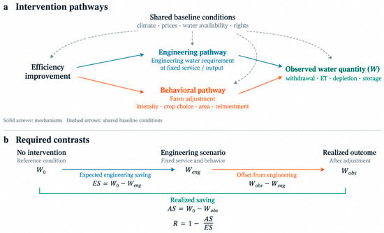
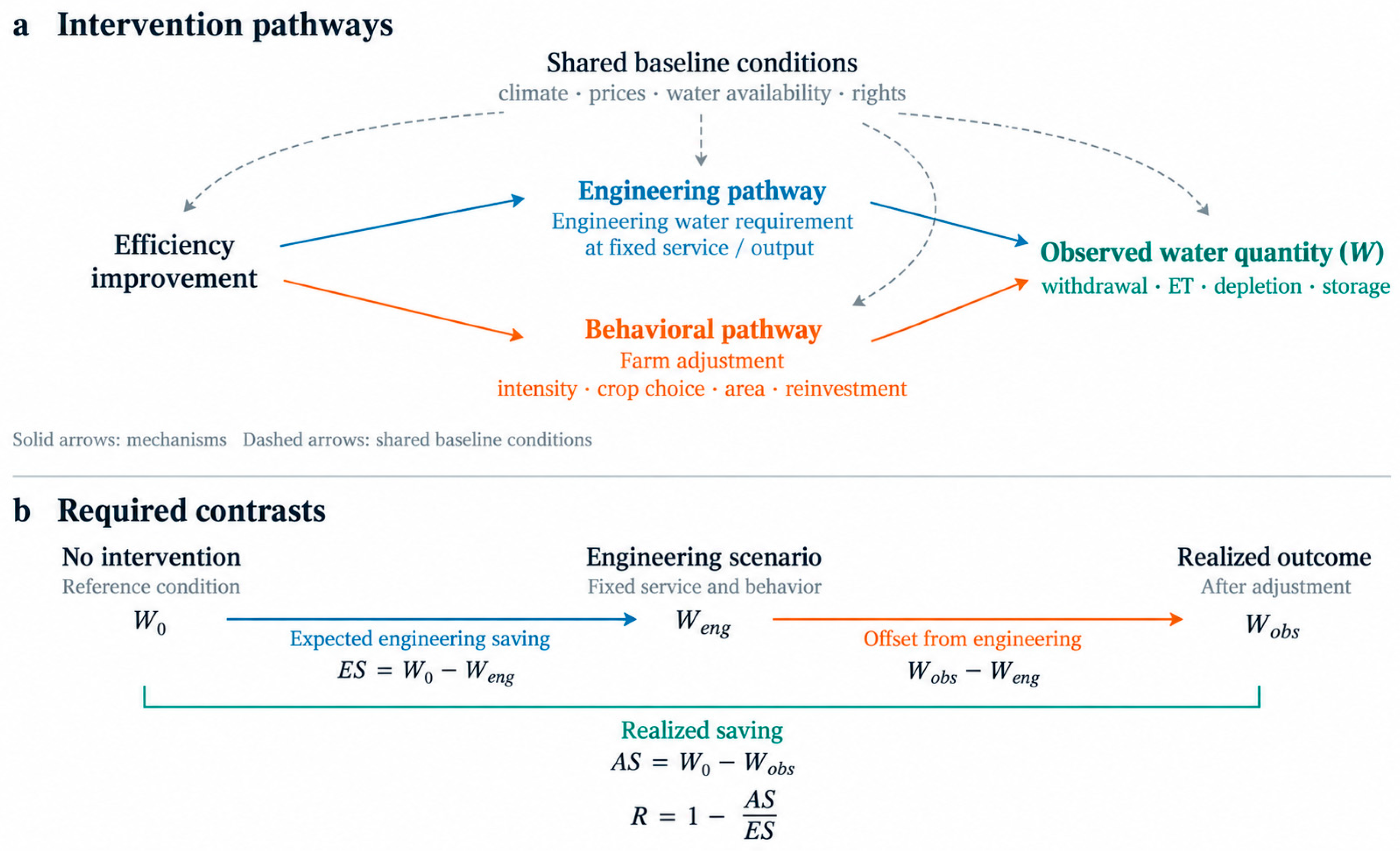
A before–after comparison generally supplies neither counterfactual. Rainfall, energy prices, crop prices, pumping lifts and allocation conditions can change between observations. Even an unbiased estimate of the intervention effect, $Q_q^1$ − $Q_q^0$, does not identify $Q_q^{\mathrm{eng}}$. For example, an experiment may establish that a subsidy did not change average pumping, but it cannot yield a numerical rebound rate unless the pumping saving expected without behavioral adjustment is also estimated. Conversely, reduced pumping relative to an untreated comparison group can coexist with partial rebound when the realized reduction is smaller than the fixed-service saving. Figure 1 relates the intervention and engineering comparisons to the observed water outcome.

Figure 1. Counterfactual framework for irrigation-water rebound. (a) Engineering and behavioral pathways following efficiency improvement. (b) Comparison of no-intervention, fixed-service engineering and realized outcomes within a common water-accounting boundary and period.

A statistically insignificant pumping effect can encompass increases and reductions within its confidence interval. Its interpretation depends on the precision of the estimate, follow-up period and expected engineering saving. A small, uncertain denominator can also produce an unstable rebound ratio. Where ES_q is close to zero, absolute changes and their uncertainty should take precedence; where ES_q = 0, the ratio is undefined. This distinction is particularly relevant when a delivery-saving intervention is evaluated using depletion.

Supply expansion changes water use through a different mechanism. A new reservoir, transfer or electricity supply can relax a production constraint without improving irrigation efficiency. Similarly, residential demand may recover after drought restrictions because conservation behavior changes [20]. Distinguishing these processes helps attribute changes in water use to the intervention examined.

2.2. Withdrawal, Consumption and Storage

Withdrawal is the volume removed from a river, aquifer or supply system; field application is the volume delivered to the field. Evapotranspiration (ET) includes evaporation and transpiration supplied by rainfall and irrigation. Irrigation consumptive use includes the irrigation-derived portion of ET and water incorporated into products. Depletion also includes flows that cannot be recovered within the defined resource account. Groundwater storage change records a change in the aquifer stock. Table 1 summarizes these quantities and the observations needed to interpret them [2,8,21].

Table 1. Water quantities used to evaluate irrigation outcomes.

Quantity	Operational Meaning	Interpretation
Withdrawal (W)	Gross abstraction or delivery crossing the selected boundary.	Measures pressure on a source or delivery system; does not subtract recoverable returns or identify total depletion.
Field application	Water reaching the field after conveyance.	Useful for engineering performance; changes in conveyance and source substitution must be assessed separately.
Evapotranspiration (ET)	Water transferred to the atmosphere through evaporation and transpiration.	Includes productive and non-productive components and may include rainfall-derived water; total ET is not automatically irrigation consumption.
Depletion (D)	ET plus physical outflow to non-recoverable sinks in the defined resource account.	Depends on the accounting boundary and whether outflows remain available for subsequent use.
Recoverable flow (Fr)	Outflow available for subsequent use within the relevant connected system.	Depends on timing, location and quality. Recharge within the account is a transfer, not an additional loss.
Storage change (ΔS)	End-of-period minus beginning-of-period water stock.	Negative values indicate stock decline. Storage change is included explicitly in the water balance.

For an irrigated control volume, a simplified accounting-period balance can be written as

W + P + I = ET + F_r + F_n + ΔS

(3)

Here, W is withdrawal or delivery crossing the selected boundary, P is precipitation, I is other inflow, ET is evapotranspiration, F_r is recoverable outflow, F_n is outflow to a non-recoverable sink, and ΔS is the end-of-period minus beginning-of-period change in storage. The example neglects water incorporated into harvested products; that term can be included where material. Within this account, depletion is

D = ET + F_n

(4)

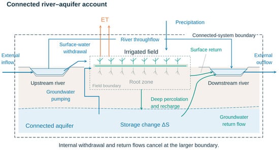
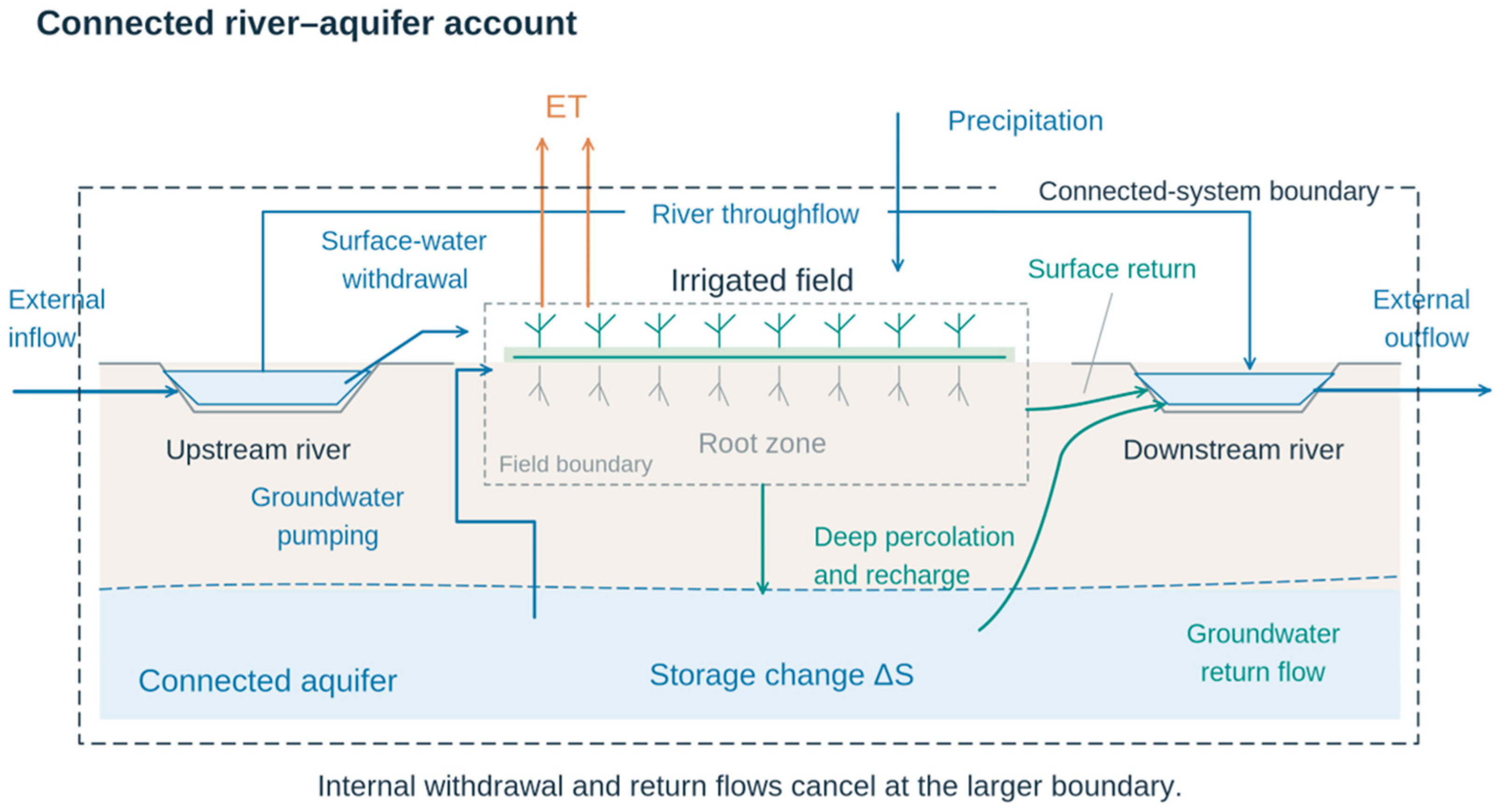
The recoverability of a flow depends on its location, timing and quality. Drainage from one farm may supply another user downstream, and recharge contributes to storage when the aquifer is inside the accounting boundary. Combining field and aquifer balances treats this recharge as an internal transfer. Storage change accounts for water retained or released during the period. Water quality can restrict subsequent use and should be considered when classifying recoverable flows. Figure 2 shows the connected field, river and aquifer account.

Figure 2. Connected field–river–aquifer water accounting. Schematic flows and storage changes across nested accounting boundaries. Based on Perry [2], Kendy and Bredehoeft [22] and Lankford [8].

Let δ denote the difference between the intervention and no-intervention outcomes, under the same external conditions. Equations (3) and (4) imply

δD = δW + δP + δI − δF_r − δ(ΔS)

(5)

Under equal precipitation and other inflows, the relation simplifies to δD = δW − δFr − δ(ΔS). A withdrawal reduction matched by an equal reduction in recoverable return flow produces no depletion saving when storage change is unchanged. The equality follows from the water balance. At a larger basin boundary, internal diversions and internal returns cancel; the relevant account then concerns external inflows and outflows, atmospheric losses, and stock changes. Outflow from an upstream district may support downstream ecosystems.

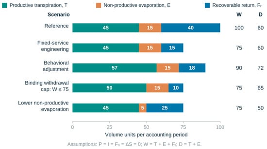
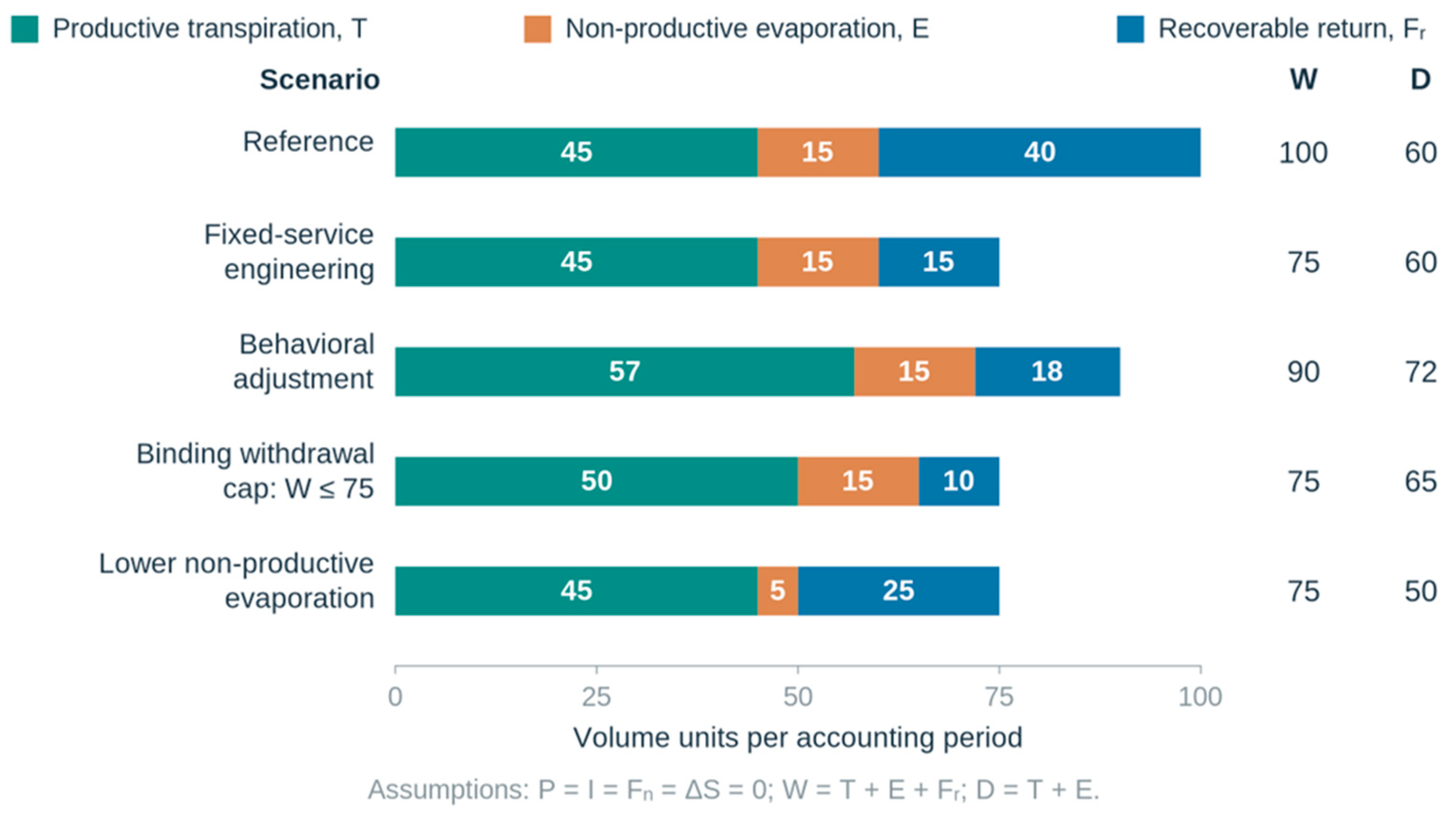
In the hypothetical scenarios in Figure 3, the reference withdrawal is 100 units, ET is 60 and recoverable return flow is 40. Fixed-service modernization reduces withdrawal to 75 and return flow to 15, leaving ET unchanged. The engineering withdrawal saving is 25, but the engineering depletion saving is zero. A behavioral scenario with withdrawal of 90, ET of 72 and returns of 18 yields a withdrawal rebound of 60%; the depletion rebound percentage remains undefined against the zero-saving engineering benchmark. The example holds other inflows and storage change fixed.

Figure 3. Water balances under hypothetical irrigation scenarios. The scenarios compare unchanged crop transpiration, behavioral adjustment, a withdrawal limit and reduced soil evaporation. Volumes are expressed in arbitrary units per accounting period; precipitation, other inflows and storage change are set to zero.

At a withdrawal limit of 75 units, ET can increase to 65 while returns fall to 10. Depletion then exceeds its reference value despite compliance with the withdrawal limit. In the lower-evaporation scenario, productive transpiration remains at 45 units while non-productive evaporation falls from 15 to 5 units, reducing depletion from 60 to 50. The savings therefore depend on which component of the water balance the intervention changes [8,23].

Separating rainfall-derived and irrigation-derived ET is necessary when evaluating irrigation consumption. Changes in crops, rainfall capture and antecedent soil moisture affect both contributions. Satellite estimates of total ET can be combined with rainfall, soil-water observations and a water-balance model to examine their sources. Seasonal estimates also reveal changes in timing that an annual total may conceal.

2.3. Behavioral Choices and Conditions for Conservation

Consider crop or rotation classes c, physical areas a_c, annual cropping intensities n_c, and applied water $w_c=\sum _i{w}_{\mathit{ci}}$ per hectare and cycle from source i. Technology τ provides effective crop-water service x_c = η_c(τ)w_c. A farmer chooses area, crop mix, intensity and water to maximize:

$${\max }_{a,n,w}\Pi ={\sum }_c{a}_c\left\{n_c\right[p_c{f}_c\left({\eta }_c{w}_c;z\right)-C_c]-k_c-j_c\left(n_c\right)\}-G\left(A\right)$$

(6)

Here, $A=\sum _c{a}_c$ is physical area; production f_c has diminishing marginal returns to effective water under contemporaneous climate and agronomy z. Variable cost C_c includes water charges, energy $p_E\sum _i{e}_{\mathit{ci}}\left(\tau ,h_i\right)w_{\mathit{ci}}$, labor p_L𝓁_c(τ,w_c) and other inputs. Pumping lift enters h_i, and annualized capital cost k_c is net of subsidy. Convex functions G and j_c represent expansion and intensification costs. These choices satisfy

$$\begin{array}{rr}A& \le \overline{A}, W_i={\displaystyle \sum _c}{a}_c{n}_c{w}_{\mathit{ci}}\le {\overline{W}}_i,\\ {\displaystyle \sum _i}{W}_i& \le W^{\mathrm{right}}+T, 0\le n_c\le {\overline{n}}_c.\end{array}$$

(7)

These are effective land, source and entitlement constraints. The authorized net rights transfer T is specified; its transaction cost enters the objective if transfers are optimized, and trading must respect the aggregate allocation. A nominal right above feasible use need not bind. For one crop and source with locally constant marginal water cost c_w, an interior choice satisfies

pηf^′(ηw) = c_w + λ_W

(8)

The shadow price λ_W represents active water constraints. Under slack constraints and downward-sloping crop-water demand, reducing the cost per unit of crop-water service raises crop-water demand. Area expands if the optimized net margin rises, given unchanged strictly convex expansion costs and interior optima. Energy and capital costs can offset labor or application benefits; a land cap still allows crop and intensity changes. Supplementary Section S3 derives the withdrawal elasticity and states the assumptions for these responses.

The condition for reduced depletion follows from the water balance. Define S_W = W⁰ − W¹, lost recoverable outflow $L_F=F_r^0-F_r^1$, and δX = X¹ − X⁰. Keeping ΔS = S_end − S_start throughout gives

S_D = S_W − L_F + K > 0,  K = −δP−δI+δ(ΔS)

(9)

Withdrawal savings reduce depletion when they exceed the reduction in recoverable outflow after accounting for changes in other inflows and storage. In the irrigation-only account with zero storage change, let u = W¹/W⁰ and $r_j=F_r^j/W^j$. The separate conditions are

withdrawal saving: u < 1;  depletion saving: u(1 − r₁) < 1 − r₀

(10)

Figure S3.1 shows all four combinations. At fixed productive service, reducing only recoverable returns can give ES_W > 0 and ES_D = 0. Reducing non-beneficial evaporation or non-recoverable outflow can instead give ES_D > 0; it survives adjustment exactly when D¹ − D^eng < ES_D. Groundwater also requires ΔS_g = R_g + L_g − W_g − Q_g. With unchanged lateral exchange and connected-stream discharge, reduced pumping must exceed lost recharge to improve the storage trajectory; absolute recovery additionally requires $\Delta S_g^1>0$.

Climate, energy and output prices, subsidies, farm structure, groundwater lift and enforcement enter distinct production, cost or constraint terms. A technology-only counterfactual holds external conditions and institutions consistent; an intervention that also changes allocations is a program effect unless its components are separately identified. Crop changes following adoption can mediate the total intervention effect. Supplementary Table S2 maps these factors to the comparative design.

2.4. Uncertainty in Engineering Savings and Return Flows

Let E = ES_q and B = AS_q. For R = 1 − B/E, sensitivity is

$${\displaystyle \frac{\partial R}{\partial E}}={\displaystyle \frac{B}{E^2}}, {\displaystyle \frac{\partial R}{\partial B}}=-{\displaystyle \frac{1}{E}}$$

(11)

The first derivative holds realized saving fixed. It vanishes at B = 0, but a small denominator still amplifies uncertainty in B. When E is separated from zero and joint covariance is available, first-order propagation gives

$$\mathrm{Var}\left(R\right)\approx {\displaystyle \frac{\mathrm{Var}\left(B\right)}{E^2}}+{\displaystyle \frac{B^2\mathrm{Var}\left(E\right)}{E^4}}-{\displaystyle \frac{2B\mathrm{Cov}\left(B,E\right)}{E^3}}$$

(12)

Both savings have the same no-intervention baseline, creating covariance between them. This approximation is unsuitable when uncertainty in the denominator reaches zero. Monte Carlo or Bayesian methods propagate uncertainty when supported by a joint model for identified counterfactuals and engineering benchmarks.

A feasible set $𝒞$ can instead retain every jointly feasible pair (E,B) and its ratio where E > 0. For separate parameter intervals E ∈ [e_L,e_U], B ∈ [b_L,b_U], e_L > 0, the exact extrema occur at its four corners:

$$\begin{array}{c}{R}_{\min }={\min }_{e\in \{e_L,e_U\},\hspace{0.17em}b\in \{b_L,b_U\}}\left(1-b/e\right),\\ R_{\max }={\max }_{e\in \{e_L,e_U\},\hspace{0.17em}b\in \{b_L,b_U\}}\left(1-b/e\right).\end{array}$$

(13)

Known dependence and physical constraints should be retained in $𝒞$. If E can approach zero, finite bounds generally require additional joint restrictions. Absolute changes and their uncertainty remain interpretable when the ratio is undefined. For any valid positive benchmark, R > 1 exactly when B < 0; a probability of either event still requires inferential evidence. Supplementary Section S3 gives a bound on changes in the ratio.

With $F_r^j=r_j{W}^j$, the depletion account and its first-order uncertainty are

$$\begin{array}{c}{S}_D=\left(1-r_0\right)W^0-\left(1-r_1\right)W^1+K,\\ \mathit{Var}\left(S_D\right)\approx g^{\mathrm{T}}\mathit{\Sigma g}.\end{array}$$

(14)

For the input vector (W⁰,W¹,r₀,r₁,𝛿P,𝛿I,𝛿(ΔS)), the gradient is g = (1 − r₀,−(1 − r₁),−W⁰,W¹,−1,−1,1). Shared data and residual flows require covariance. Storage uncertainty includes covariance between the beginning and end stocks. For a linear balance in the flow quantities, covariance propagation is exact.

Sensitivity calculations in Supplementary Section S3 illustrate how assumed input ranges affect the results. For the Figure 3 example, ES_W ∈ [20,30] and AS_W ∈ [8,12] give R_W ∈ [0.400,0.733]. In the Spanish historical comparison, varying each return fraction by ±0.02 gives a difference of 131.88–1444.12 hm³/year; varying each by ±0.03 gives −196.18–1772.18 hm³/year. In Idaho, a ±5% change in the reported reduction in net reach gain gives a difference of −2.95–26.95 Mm³/year between the reductions in diversion and reach gain. These perturbations bracket the sign-change thresholds: ±2.40 percentage points in the Spanish return fractions and ±4.01% in the Henrys Fork reach-gain reduction, with the remaining inputs held fixed.

3. Empirical Evidence and Recurrent Mechanisms

3.1. Groundwater Irrigation: Adoption, Constraints and Conflicting Estimates

Groundwater studies are particularly informative because metered abstraction can be linked to technology, crops and land at relatively fine scales. In western Kansas, conversion from conventional center-pivot to dropped-nozzle systems was initially associated with increased extraction rather than the intended reduction; crop changes contributed to the response [11]. Subsequent analysis found that responses to low-energy precision application depended on water-right size, with greater scope for additional use under less restrictive allocations [12]. Together, these studies illustrate the importance of the intensive and extensive margins, but their measured outcome is pumping, not a complete aquifer or basin water balance.

The later reassessment by Cameron-Harp and Hendricks changes the interpretation of this evidence. Comparing flood/furrow-to-center-pivot transitions during 1991–2015 and traditional-center-pivot-to-low-energy-precision-application transitions during 1991–2019, it shows that conventional two-way fixed-effects estimates can misrepresent effects when adoption is staggered and responses evolve. Estimation appropriate to these conditions found no statistically significant evidence of backfire for either transition [13]. This shows that technology transitions should be distinguished and that comparisons among already-treated and newly treated irrigators can produce misleading averages. Modern difference-in-differences methods estimate adoption effects while allowing responses to differ across cohorts and time [24,25].

The Kansas studies examine related agricultural and hydrological settings, with different samples, periods and technology comparisons. Farm structure offers an additional explanation for changes in extraction: Ao et al. found an association between farm growth and groundwater depletion in the Kansas High Plains [26]. Comparing these studies therefore requires separating equipment adoption from changes in farm scale and resource availability.

The South India experiment examined a randomized offer of assistance and additional drip-irrigation subsidy. Production and groundwater transfers changed, while reported pump-operation duration showed no statistically significant change between the 2016 baseline and 2019 follow-up [14]. Electricity rationing constrained pumping, and farmers could transfer water to neighboring plots. Thus, adjustment occurred partly through production and transfers within the existing pumping constraint. Pumping duration was used because volumetric metering was impractical; conversion to water volume depends on discharge rates.

A survey of 404 micro-irrigation adopters across four Indian states recorded a 267 ha increase in recalled irrigated area, equivalent to 17%, alongside generally shorter pumping duration [27]. This pattern links adoption to area expansion and changes in cropping. The survey describes changes reported by adopters, whereas the South India experiment estimates the effect of a subsidy offer under electricity rationing. Together, they identify area, production and water transfers as responses that may accompany changes in application per hectare.

Groundwater simulations for India examine how expansion changes the technical potential for conservation [28]. Savings decline when water released by improved efficiency supports additional irrigated production. Across these studies, expansion is more likely where land and water remain available, while binding pumping constraints redirect adjustment toward production or transfers. The technology and the conditions governing its use jointly determine the water outcome.

3.2. Modernization at Farm and Irrigation-District Scales

District modernization often combines canal rehabilitation, pressurization, delivery schedules, financing and allocation changes. More reliable supply can support new crops, lower labor requirements can facilitate larger operations, and irrigation associations can redistribute water released by these changes. Spanish studies relate the resulting water use to initial irrigation deficits, available land and water allocations [5,17,23,29,30]. Fixed-area models isolate changes in application and crop-water supply; program evaluations capture the combined effects of technology, infrastructure and management.

In Australia, Wheeler et al. analyzed 2481 irrigation-survey records, with 1604 observations in the principal adjusted sample. Grant recipients extracted 21–28% more water than surveyed non-recipients across adjusted estimators [31]. Regression adjustment, inverse-probability weighting and matching accounted for observed farmer, farm and year characteristics. This result links infrastructure support to greater extraction among recipients; the net resource effect also depends on selection into the program and the allocation of recovered entitlements. Drought and supply reliability influence this response because improved infrastructure can sustain production under restricted allocations and permit expansion when allocations increase [32].

In Morocco, modernization policy combined water-conservation objectives with the expansion of higher-value irrigated production [33]. The allocation rules and incentives determining land and water use shaped the tension between these goals. Stakeholders in Uzbekistan also anticipated opportunities for increased production following irrigation improvements [34]. These studies explain how policy objectives and users’ expectations influence adoption and subsequent management.

In the Henrys Fork watershed, Idaho, a comparison of 1978–2000 with 2001–2022 found annual reductions of 311 Mm³ in surface-water diversion and 299 Mm³ in net river reach gain [35]. The similar magnitudes link reduced diversions to changes in groundwater-supported river flows. Net reach gain combines river–aquifer exchanges, so the 12 Mm³/year difference between these reductions represents only part of the connected water balance. Climate, pumping, storage and other exchanges are needed to interpret the remaining change.

The spatial distribution of these changes matters for downstream users. Spanish irrigation–wetland studies show that drip adoption can accompany changes in allocation and wetland dependence on irrigation flows [36]. Reduced delivery may leave more water in an upstream reach while decreasing recharge and later groundwater discharge elsewhere. Table 2 compares the designs and water quantities used to examine these outcomes.

Table 2. Research designs and water measurements in the selected studies.

Evidence Class	Selected Studies	Comparison or Estimand	Design Considerations	Water Measurements
Randomized encouragement	Fishman et al. [14]	Effect of the subsidy-support offer; adoption effect requires additional assumptions.	Noncompliance and transfer effects must be distinguished from assignment.	Reported pumping duration; volume estimates additionally depend on discharge.
Quasi-experimental policy or adoption comparison	Cameron-Harp and Hendricks [13]; Drysdale and Hendricks [37]	Effects for specific technology transitions or policies, conditional on the comparison design.	Pre-trends, adoption timing, control eligibility and spillovers matter.	Withdrawal, irrigated area and application depth; aquifer response also depends on recharge and exchange.
Selection-adjusted observational analysis	Pfeiffer and Lin [11]; Li and Zhao [12]; Wheeler et al. [31]	Adoption or recipient contrasts conditional on covariate/design assumptions.	Unobserved selection and bundled changes may remain.	Extraction at the source; basin effects depend on return flows and consumption.
Historical, survey or decomposition evidence	Singh et al. [27]; Morrisett et al. [35]; Song et al. [38]; Xu et al. [39]; Pei et al. [40]; Espinosa-Tasón et al. [41]	Recorded or reconstructed changes and accounting components.	No isolated technology effect from before–after change or decomposition alone.	Reported or reconstructed flows and production indicators, with study-specific definitions.
Analytical and simulation scenarios	Berbel and Mateos [17]; Berbel et al. [23]; Fishman et al. [28]; Freire-González [42]; Zhou et al. [43]	Conditional outcomes under a production model or an imposed policy/efficiency scenario.	Conclusions depend on behavioral assumptions, calibration and closure.	Modeled withdrawals, consumption, returns and storage within the stated system.
Qualitative and institutional explanation	Molle and Tanouti [33]; Hamidov et al. [34]	Institutional incentives, stakeholder perceptions and possible pathways.	Mechanism/context evidence, without a transferable treatment-effect magnitude.	Stakeholder perceptions and institutional processes relevant to water use.

3.3. Regional and Economy-Wide Water-Use Responses

Regional studies identify land and cropping changes that accompany agricultural water-use efficiency. Song et al. examine scale and crop-structure components of agricultural water use in China [38]. Using 30 provinces during 2000–2017, Xu et al. report an efficiency-based rebound estimate of 88.81%; area expansion was associated with increased water use, whereas changes in crop composition were associated with lower use [39]. Pei et al. report a rebound estimate of 112.10% for Xinjiang during 2001–2020, alongside expansion of cultivated and irrigated land [40]. In the Hetao Irrigation District, Xu and Song identify expansion of sown area and the irrigated share of land as the main contributions to increased water use over 1949–2017 [44]. Climate and crop mix further modify these relationships [45]. The estimates use different efficiency measures and comparisons; their definitions and results are recorded separately in Supplementary Table S1.

Regional efficiency measures often share water inputs with the outcome being explained. An output-to-water ratio can improve through higher output, lower water input, price changes or a different crop composition. Decomposition separates the contributions of these components, while attribution to a technology change additionally depends on the comparison design. This distinction is particularly relevant when long-term trends in land use and production accompany irrigation investment.

Regional and farm-level studies therefore describe different scales of adjustment. Provincial estimates include changes in crops, land and markets over time; well-level adoption studies focus on particular technology transitions. The regional evidence helps identify expansion and restructuring mechanisms, while local studies examine their relation to adoption and resource constraints. Comparing them by intervention, water quantity and period explains differences more clearly than pooling their reported percentages.

Economy-wide models examine adjustments through production, prices and demand across sectors. Freire-González uses a dynamic water-economy model to examine improved water productivity in Spain [42]. Zhou et al. compare short- and long-run responses in a multi-sector Chinese model [43]. Their water account uses efficiency units to represent delivered water services. In the short run, wages and sectoral capital stocks are fixed and employment adjusts; in the long run, capital moves across sectors, rates of return converge, and wages adjust at fixed employment. These assumptions determine how efficiency gains affect production and water demand.

Hydrological and hydro-economic models connect these responses to water flows. Integrated agricultural simulations track changes in ET, recharge and returns [46], while hydro-economic models represent production decisions and allocation constraints within a water balance [47]. The iGains4Gains model compares irrigation and allocation scenarios across water, food, carbon and nature outcomes [48]. Ilyas et al. couple water-balance adjustment with rent-seeking behavior, showing how institutional responses can reduce a modeled efficiency benefit [49]. These models complement observations by examining how specified behavioral and hydrological mechanisms interact.

3.4. Irrigation Outcomes Across Regional Settings

Additional cases from sub-Saharan Africa and Southeast Asia extend the comparison of interventions and accounting boundaries. In northern Benin, Burney et al. evaluated a solar-pumping and drip-irrigation package in two intervention villages and two matched comparison villages over its first year [50]. Hand-watered comparison gardens identify the bundled intervention against existing practice, with livelihood and food-security outcomes. In the Philippine UPRIIS rice system, Hafeez et al. documented reuse at several spatial levels [51], demonstrating how field outflows become inputs elsewhere in the irrigation system.

The companion UPRIIS report monitored 158 surface-flow boundary points twice daily, estimated pumping from discharge rates and operating times, and modeled ET with SEBAL [52]. Its 18,003 ha account ended at the root-zone base; the lower-boundary flux was calculated as the residual, with soil-water storage change assumed negligible. These measurements describe how reuse connects fields and irrigation-system boundaries and identify the terms estimated from the balance.

Transferability depends on initial water stress, source connectivity, electricity and crop prices, land and credit access, subsidy design, pumping lift and allocation enforcement (Supplementary Table S2). In water-constrained systems, efficiency gains may improve production or reliability. Extensive downstream reuse increases the importance of recoverable flows, while effective depletion limits and reduced non-beneficial evaporation can protect conservation benefits. These conditions explain why similar technologies can produce different resource outcomes across regions. Evidence from settings with greater unmet irrigation demand would give more weight to production expansion, while evidence from systems with little recoverable drainage would give more weight to depletion savings. These differences would affect the relative importance of the mechanisms in the synthesis.

3.5. Comparison of Reported Water-Use Changes

Supplementary Table S5 compares the definitions and available inputs for six studies of technology adoption, infrastructure support and water-use change. For a common water quantity, boundary, population and period, define $a_q=\left(Q_q^0-Q_q^1\right)/Q_q^0$ and $e_q=\left(Q_q^0-Q_q^{\mathrm{eng}}\right)/Q_q^0$, with $Q_q^0>0$. Positive a_q denotes attributable saving; R_q = 1 − a_q/e_q additionally requires a positive engineering saving for the same crop-water service. Realized outcomes retain area and intensity responses; normalizing by post-adoption area would estimate a different effect.

The comparisons in Table S5 show how technology effects and historical water-use changes differ. In Spain, abstraction, estimated consumption and derived returns declined by 15.78%, 7.12% and 29.99%, respectively [41]. The Australian extraction difference of 21–28% summarizes adjusted estimates from the same survey [31]. The Kansas estimates describe annual withdrawal changes for two distinct irrigation transitions [13]. Together with the South India experiment, the Henrys Fork account and the Spanish economy-wide model, these cases relate observed water use to adoption, allocation and hydrological setting.

Allocation constraints, hydrological connectivity and return fractions help explain differences among these results. Comparisons within a study are particularly useful because they hold parts of the setting and measurement design constant. The synthesis examines these conditions qualitatively and interprets estimates from shared samples together.

4. From Efficiency Gains to Conservation Outcomes

4.1. Quantitative Limits, Water Rights and the Allocation of Savings

Governance determines which uses remain feasible after efficiency improves, but the existence of a legal instrument is not sufficient evidence that it constrains behavior. A nominal allocation above historical or feasible use can leave ample room for intensification. A restriction on irrigated area can still permit higher irrigation intensity or a longer growing season. Conversely, a binding pumping limit can channel a productivity gain into higher output or transfers without increasing extraction. The relevant institutional variable is thus the effective constraint facing users, not simply whether a water-right system or a modernization subsidy is present [12,14].

A locally governed Kansas allocation program reduced water use by an estimated 26%, mainly through lower irrigation intensity [37]. This finding shows how a binding allocation can change pumping while allowing farmers to adjust production. The intervention was a water-use restriction; its effects provide a comparison for technology programs operating under different limits. The resulting aquifer response depends on recharge, lateral flows and storage over time.

Chinese water-right evaluations report different responses to reform. Fei et al. found an increase in their estimated agricultural rebound measure following the pilot reform [53], whereas Sheng et al. report mitigation under a water-rights-trading policy, with effects varying across settings [54]. The policies changed different allocation arrangements and used different outcome measures. Their comparison highlights the importance of the entitlement transferred, enforcement and the way changes in water use are measured.

A limit on irrigation withdrawals may leave depletion unchanged if return flows decline. It can also permit greater consumption within the same withdrawal allowance when cropping or irrigation intensity changes. Evaluating an allocation rule therefore requires relating the controlled withdrawal to consumption, return flows and storage in the affected system. Figure 4 illustrates this relationship using the Spanish historical comparison and sensitivity to assumed return fractions.

Espinosa-Tasón et al. [41] estimated that Spanish irrigation abstraction declined from 17,808 to 14,998 hm³/year between 2004 and 2017 (−15.8%). Estimated consumption declined from 11,065 to 10,277 hm³/year (−7.1%), and returns, calculated as abstraction minus consumption, fell from 6743 to 4721 hm³/year (−30.0%). Application efficiency increased from 0.76 to 0.80, while irrigated area expanded from 3.264 to 3.734 Mha. The 2810 hm³/year reduction in abstraction thus comprised a 788 hm³/year reduction in estimated consumption and a 2022 hm³/year reduction in derived returns. Figure 4b shows how varying the return fractions changes this calculated consumption difference. The comparison describes historical changes in the national account, including concurrent changes in climate, crops, area and water sources.

Figure 4. Changes in Spanish irrigation-water use and sensitivity to return-flow assumptions. (a) Annual abstraction, estimated consumption and derived returns in 2004 and 2017, from Espinosa-Tasón et al. [41], Table 3. (b) Range of the calculated consumption difference when the two return fractions vary separately by the indicated number of percentage points, with abstraction and other water-balance terms held fixed. Supplementary Section S3.6 provides the calculations.

Figure 4. Changes in Spanish irrigation-water use and sensitivity to return-flow assumptions. (a) Annual abstraction, estimated consumption and derived returns in 2004 and 2017, from Espinosa-Tasón et al. [41], Table 3. (b) Range of the calculated consumption difference when the two return fractions vary separately by the indicated number of percentage points, with abstraction and other water-balance terms held fixed. Supplementary Section S3.6 provides the calculations.

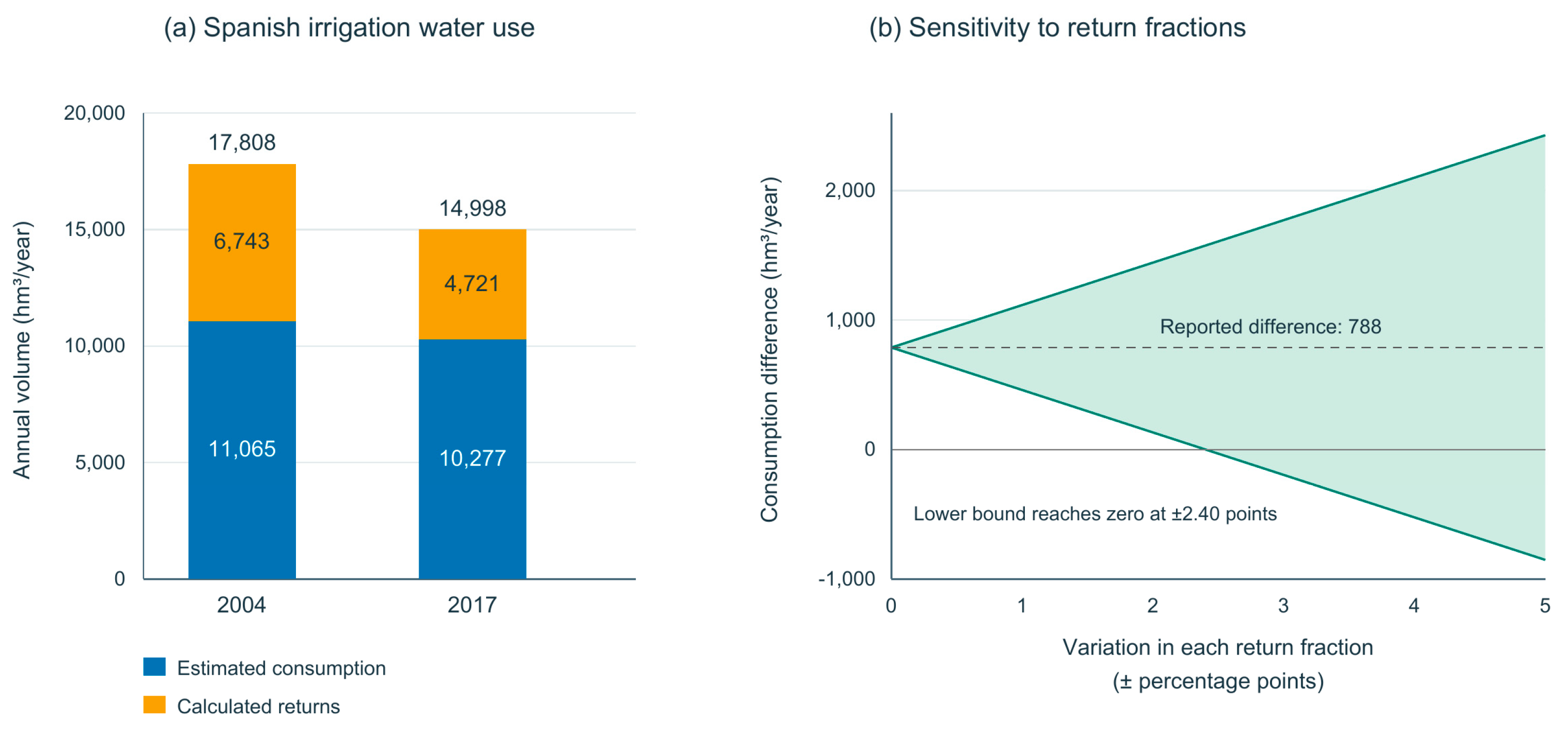
Table 3. Water measurements relevant to six irrigation-management objectives.

Objective	Minimum Indicators	Suggested Observation and Review Schedule	Lead and Supporting Participants	Use in Evaluation
Lower groundwater abstraction	Metered well volume, legal allocations, source substitution and an intervention baseline.	Record each pumping event or use continuous meters; reconcile totals monthly and at allocation review.	Lead: water regulator. Support: well operators and independent auditors.	Estimate the pumping change attributable to the intervention and account for transfers.
Aquifer recovery	Groundwater heads and storage conversion, pumping, recharge and connected-river exchange.	Measure heads monthly at sentinel wells; review seasonal storage and annual trends.	Lead: groundwater agency. Support: hydrologists and local users.	Relate changes in groundwater levels to storage, recharge and exchange.
Lower basin depletion	Source-partitioned ET or a bounded balance, recoverable outflows, inflows and ΔS.	Aggregate ET and flow data monthly during irrigation; reconcile the annual balance.	Lead: basin authority. Support: monitoring and remote-sensing teams.	Estimate depletion changes after accounting for recoverable flows and storage.
Protect environmental flow	Discharge at the named reach and season, quality, reservoir operations and re-diversion.	Monitor critical-reach discharge continuously; review compliance during the ecological season.	Lead: river/environment agency. Support: reservoir operators and downstream users.	Assess whether water reaches the ecosystem at the required time and quality.
Recover water through public subsidy	Verified eligible baseline, equipment/area/crop records, water quantity and disposition of the benefit.	Establish a pre-program baseline; verify each irrigation season and before payment.	Lead: funding body. Support: basin regulator, independent verifier and farmer representatives.	Relate public expenditure to additional water available for the stated purpose.
Improve productivity and adaptation	Yield, income, reliability, labor and environmental effects reported separately.	Record yield, income and labor each crop season; compare outcomes across weather conditions.	Lead: agricultural agency. Support: user associations and representative smallholders.	Compare production and income outcomes with their water-resource effects.

Table 3. Water measurements relevant to six irrigation-management objectives.

Objective	Minimum Indicators	Suggested Observation and Review Schedule	Lead and Supporting Participants	Use in Evaluation
Lower groundwater abstraction	Metered well volume, legal allocations, source substitution and an intervention baseline.	Record each pumping event or use continuous meters; reconcile totals monthly and at allocation review.	Lead: water regulator. Support: well operators and independent auditors.	Estimate the pumping change attributable to the intervention and account for transfers.
Aquifer recovery	Groundwater heads and storage conversion, pumping, recharge and connected-river exchange.	Measure heads monthly at sentinel wells; review seasonal storage and annual trends.	Lead: groundwater agency. Support: hydrologists and local users.	Relate changes in groundwater levels to storage, recharge and exchange.
Lower basin depletion	Source-partitioned ET or a bounded balance, recoverable outflows, inflows and ΔS.	Aggregate ET and flow data monthly during irrigation; reconcile the annual balance.	Lead: basin authority. Support: monitoring and remote-sensing teams.	Estimate depletion changes after accounting for recoverable flows and storage.
Protect environmental flow	Discharge at the named reach and season, quality, reservoir operations and re-diversion.	Monitor critical-reach discharge continuously; review compliance during the ecological season.	Lead: river/environment agency. Support: reservoir operators and downstream users.	Assess whether water reaches the ecosystem at the required time and quality.
Recover water through public subsidy	Verified eligible baseline, equipment/area/crop records, water quantity and disposition of the benefit.	Establish a pre-program baseline; verify each irrigation season and before payment.	Lead: funding body. Support: basin regulator, independent verifier and farmer representatives.	Relate public expenditure to additional water available for the stated purpose.
Improve productivity and adaptation	Yield, income, reliability, labor and environmental effects reported separately.	Record yield, income and labor each crop season; compare outcomes across weather conditions.	Lead: agricultural agency. Support: user associations and representative smallholders.	Compare production and income outcomes with their water-resource effects.

The allocation of saved water determines who receives its benefits. Farmers may use it on other fields, transfer it to another user or leave it available for environmental purposes. Where public funding aims to recover water for ecosystems or aquifers, the relevant saving is the reduction relative to water use expected without the program. Retiring unused entitlements produces a different outcome from reducing existing consumptive use. Transfer and reuse rules therefore influence both the environmental benefit and its distribution [6,7].

Users’ expectations also influence the feasibility of these arrangements. Spanish irrigation associations may regard savings as returns to their investment, while funding agencies expect environmental benefits. Research on mental accounting and coordination among governance actors documents these differences in expectations and administrative relationships [55,56]. Institutional arrangements depend on local hydrology, monitoring capacity and the users involved [57,58].

4.2. Source Substitution, Return Flows and Environmental Protection

Substitution between water sources can redistribute the effects of an irrigation policy. Farmers may replace lower canal deliveries with groundwater, or use additional surface water as pumping declines. These changes affect aquifer storage, pumping costs, subsidence and river flows in different ways. Evaluation across the connected system can identify both the benefit to the targeted source and changes elsewhere [2,22].

Reduced seepage or deep percolation can change groundwater discharge after a delay, whereas reduced diversion can increase river flow immediately. In Henrys Fork, the principal fitted change in diversion occurred between 2000 and 2001, and the change in net reach gain between 2002 and 2003; lower-Teton users rely on reach gains during midsummer [35]. This timing means that annual irrigation-district totals can conceal changes in the season and location of downstream supply. Stream–aquifer observations over the relevant response period are needed to evaluate these effects [22,35].

Environmental benefits depend on water reaching the relevant ecosystem at the required time and quality. Reservoir operations, intervening diversions and transfers can redirect water saved upstream. Reduced drainage may improve water quality while decreasing supplies to wetlands. Environmental-flow studies and recent syntheses document these connections between irrigation management and ecological outcomes [10,36,59]. The value of a return flow therefore depends on its use and effects in the receiving system.

Reducing non-productive evaporation or outflow to non-recoverable sinks can reduce depletion. The resulting benefit depends on effects on crop production, salinity management and other water users [1,8,21].

4.3. Evaluation and Allocation Under Uncertainty

Intervention comparisons and water-balance observations answer complementary questions about conservation. Metered withdrawals, crop and technology histories, remotely sensed ET, return flows and groundwater levels can link changes in farm decisions to resource outcomes. Specifying which quantities are measured and which are modeled helps identify the observations needed to evaluate the proposed mechanism.

The observation period should cover the adjustments relevant to the intervention. Application may change before farmers alter perennial crops, leasing, wells or water trading. Event-time estimates can show these responses and their uncertainty. For staggered adoption, estimators allowing heterogeneous effects account for differences among adoption cohorts [13,24,25]. Comparisons also need to consider whether neighboring users are affected by transfers or connected water flows.

Allocation under uncertainty extends this evaluation framework to management. Yang et al. (2026) combine fractional programming, Monte Carlo analysis and scenario reoptimization for irrigation-water allocation in the Fendong Irrigation District [60]. Their supply scenarios vary the available-water upper bound and aggregate efficiency parameter, linking utilization efficiency with shortage performance. The approach shows how allocation can be updated as the estimated supply changes. For the conservation objectives examined here, this planning mechanism can incorporate explicit depletion, storage and downstream-flow constraints alongside agricultural benefits. Gong et al. provide a complementary interval-programming approach incorporating effective precipitation, crop-water requirements and conjunctive supply [61].

Let u denote allocation and operating decisions, ω the joint hydrological and behavioral state, and Ω a set of hydrological and behavioral conditions considered in allocation. The following resource constraints can be incorporated into an allocation model that maximizes net agricultural benefit:

$$D\left(u,\omega \right)\le \overline{D}, S_T\left(u,\omega \right)\ge S_{\min }, Q_{j,t}\left(u,\omega \right)\ge Q_{j,t}^{\mathrm{env}} \forall \omega \in \mathsf{\Omega }$$

(15)

These constraints limit depletion and maintain minimum end-period storage and flow at reach j and time t. Ranges over Ω support decisions when probability distributions are unavailable; a joint probability model permits chance constraints with tolerances tied to the consequences of failure. Updated observations of inflows, ET, groundwater storage and downstream discharge revise the estimated supply and the conditions represented by Ω. When a revised estimate exceeds a depletion limit or falls below a storage or flow minimum, the allocation is recalculated subject to the same resource constraints.

Before investment, estimates of crop-water requirements, withdrawals, return flows and likely behavioral responses can be used to compare conservation outcomes. Parameter ranges help identify whether plausible changes in assumptions alter the preferred option. Monitoring after implementation can then update the water balance and inform subsequent allocation.

During implementation, metering, ET estimates and river or groundwater observations can be combined at the scale of the management objective. Table 3 summarizes the quantities relevant to six objectives and the timing needed to observe their response. Shared monitoring can spread equipment, calibration, maintenance and data-processing costs across farms. The schedules in Table 3 are proposed starting points for monitoring; local response times and management needs determine their implementation.

Efficiency and conservation policies can distribute benefits and costs differently. Limits on expansion may protect a shared aquifer while reducing an adopter’s private return. Payments based on nominal savings may favor farms with larger documented entitlements, while downstream users bear the effects of reduced return flows. Water rights, credit access, infrastructure and participation in collective decisions influence this distribution [33,57,58]. Production, income and downstream water availability therefore belong alongside aggregate water use in the evaluation.

Modernization can be valuable for productivity and reliability even where it produces little basin water saving. Programs intended to recover water additionally need evidence that the specified resource benefit is achieved. Linking payments or allocation changes to measured outcomes allows adjustment when water-source substitution or return-flow changes emerge. This distinction between agricultural and environmental objectives supports more targeted design of irrigation investment.

Measurement precision and resolution influence the outcomes that can be evaluated. In the United States, OpenET had a cropland ensemble mean absolute error of approximately 16 mm per month, or 17% of observed ET [62]. Local performance depends on crops, season, cloud cover and temporal reconstruction. In five irrigation schemes evaluated in 2020, WaPOR products at 100 and 250 m smoothed variation between plots, particularly below 2 ha; even 30 m data could be insufficient for the smallest plots [63]. These findings support matching field or group boundaries to the effective observation scale.

Rainfall, irrigation and storage observations help distinguish the sources of ET. Discharge measurements at drainage boundaries describe return-flow volumes when interpreted with water quality and downstream reuse; calibration and maintenance affect their accuracy [64]. Groundwater returns require observations over the longer response period of the connected aquifer and river. Supplementary Section S5 describes how these measurements can be combined in future field evaluations.

5. Conclusions

Irrigation efficiency improvements produce different water outcomes across technologies and settings. Groundwater studies show expansion, changes in cropping and transfers, with pumping responses shaped by allocation and energy constraints. District and basin studies show how reduced return flows can offset withdrawal savings, while lower non-beneficial evaporation can reduce depletion. These findings explain why improved farm performance and basin conservation do not always occur together.

The farm model identifies increased net returns as a driver of expansion when land and water constraints permit adjustment. The connected water balance shows that depletion falls when withdrawal savings exceed lost recoverable flows, after allowing for other inflows and storage change. Allocation determines whether the released water supports further production, other users or environmental flows.

Sustainable irrigation management combines productive and reliable agriculture with protection of aquifers and downstream ecosystems. Intervention comparisons establish how users respond, and connected water accounts establish where the resulting water goes. Sensitivity analysis identifies the assumptions that most affect estimated savings and can guide additional measurement. Relating these findings to allocation rules and the distribution of benefits helps assess whether modernization improves agricultural outcomes while maintaining water availability over time.

References

- Perry, C.; Steduto, P.; Allen, R.G.; Burt, C.M. Increasing productivity in irrigated agriculture: Agronomic constraints and hydrological realities. Agric. Water Manag. 2009, 96, 1517–1524. [Google Scholar] [CrossRef] [Scilit]
- Perry, C. Accounting for water use: Terminology and implications for saving water and increasing production. Agric. Water Manag. 2011, 98, 1840–1846. [Google Scholar] [CrossRef] [Scilit]
- Grafton, R.Q.; Williams, J.; Perry, C.J.; Molle, F.; Ringler, C.; Steduto, P.; Udall, B.; Wheeler, S.A.; Wang, Y.; Garrick, D.; et al. The paradox of irrigation efficiency. Science 2018, 361, 748–750. [Google Scholar] [CrossRef] [Scilit] [PubMed]
- Ward, F.A.; Pulido-Velazquez, M. Water conservation in irrigation can increase water use. Proc. Natl. Acad. Sci. USA 2008, 105, 18215–18220. [Google Scholar] [CrossRef] [Scilit] [PubMed]
- Berbel, J.; Gutiérrez-Martín, C.; Rodríguez-Díaz, J.A.; Camacho, E.; Montesinos, P. Literature review on rebound effect of water saving measures and analysis of a Spanish case study. Water Resour. Manag. 2015, 29, 663–678. [Google Scholar] [CrossRef] [Scilit]
- Pérez-Blanco, C.D.; Hrast-Essenfelder, A.; Perry, C. Irrigation technology and water conservation: A review of the theory and evidence. Rev. Environ. Econ. Policy 2020, 14, 216–239. [Google Scholar] [CrossRef] [Scilit]
- Pérez-Blanco, C.D.; Loch, A.; Ward, F.; Perry, C.; Adamson, D. Agricultural water saving through technologies: A zombie idea. Environ. Res. Lett. 2021, 16, 114032. [Google Scholar] [CrossRef] [Scilit]
- Lankford, B.A. Resolving the paradoxes of irrigation efficiency: Irrigated systems accounting analyses depletion-based water conservation for reallocation. Agric. Water Manag. 2023, 287, 108437. [Google Scholar] [CrossRef] [Scilit]
- Yao, J.; Zhang, W.; Li, S.; Xiao, P.; Berbel, J. The irrigation efficiency paradox: A critical synthesis of the rebound effect from hydrological mechanisms to transformative governance. Water 2026, 18, 802. [Google Scholar] [CrossRef] [Scilit]
- Ruffing, C.M.; Freed, Z. Irrigation efficiency and water conservation: Aligning outcomes for people and nature. Front. Water 2026, 8, 1839103. [Google Scholar] [CrossRef] [Scilit]
- Pfeiffer, L.; Lin, C.-Y.C. Does efficient irrigation technology lead to reduced groundwater extraction? Empirical evidence. J. Environ. Econ. Manag. 2014, 67, 189–208. [Google Scholar] [CrossRef] [Scilit]
- Li, H.; Zhao, J. Rebound effects of new irrigation technologies: The role of water rights. Am. J. Agric. Econ. 2018, 100, 786–808. [Google Scholar] [CrossRef] [Scilit]
- Cameron-Harp, M.V.; Hendricks, N.P. Efficiency and water use: Dynamic effects of irrigation technology adoption. J. Assoc. Environ. Resour. Econ. 2025, 12, 285–312. [Google Scholar] [CrossRef] [Scilit] [PubMed]
- Fishman, R.; Giné, X.; Jacoby, H.G. Efficient irrigation and water conservation: Evidence from South India. J. Dev. Econ. 2023, 162, 103051. [Google Scholar] [CrossRef] [Scilit]
- Page, M.J.; McKenzie, J.E.; Bossuyt, P.M.; Boutron, I.; Hoffmann, T.C.; Mulrow, C.D.; Shamseer, L.; Tetzlaff, J.M.; Akl, E.A.; Brennan, S.E.; et al. The PRISMA 2020 statement: An updated guideline for reporting systematic reviews. BMJ 2021, 372, n71. [Google Scholar] [CrossRef] [Scilit] [PubMed]
- van der Kooij, S.; Zwarteveen, M.; Boesveld, H.; Kuper, M. The efficiency of drip irrigation unpacked. Agric. Water Manag. 2013, 123, 103–110, Erratum in Agric. Water Manag. 2013, 127, 124–126. https://doi.org/10.1016/j.agwat.2013.06.012.. [Google Scholar] [CrossRef] [Scilit]
- Berbel, J.; Mateos, L. Does investment in irrigation technology necessarily generate rebound effects? A simulation analysis based on an agro-economic model. Agric. Syst. 2014, 128, 25–34. [Google Scholar] [CrossRef] [Scilit]
- Chan, N.W.; Gillingham, K. The microeconomic theory of the rebound effect and its welfare implications. J. Assoc. Environ. Resour. Econ. 2015, 2, 133–159. [Google Scholar] [CrossRef] [Scilit]
- Sorrell, S.; Dimitropoulos, J.; Sommerville, M. Empirical estimates of the direct rebound effect: A review. Energy Policy 2009, 37, 1356–1371. [Google Scholar] [CrossRef] [Scilit]
- Nemati, M.; Tran, D.; Schwabe, K. Residential water conservation and the rebound effect: A temporal decomposition and investigation. Water Resour. Res. 2023, 59, e2022WR032169. [Google Scholar] [CrossRef] [Scilit]
- Gómez, C.M.; Pérez-Blanco, C.D. Simple myths and basic maths about greening irrigation. Water Resour. Manag. 2014, 28, 4035–4044. [Google Scholar] [CrossRef] [Scilit]
- Kendy, E.; Bredehoeft, J.D. Transient effects of groundwater pumping and surface-water-irrigation returns on streamflow. Water Resour. Res. 2006, 42, W08415. [Google Scholar] [CrossRef] [Scilit]
- Berbel, J.; Gutiérrez-Martín, C.; Expósito, A. Impacts of irrigation efficiency improvement on water use, water consumption and response to water price at field level. Agric. Water Manag. 2018, 203, 423–429. [Google Scholar] [CrossRef] [Scilit]
- Callaway, B.; Sant’Anna, P.H.C. Difference-in-differences with multiple time periods. J. Econom. 2021, 225, 200–230. [Google Scholar] [CrossRef] [Scilit]
- Sun, L.; Abraham, S. Estimating dynamic treatment effects in event studies with heterogeneous treatment effects. J. Econom. 2021, 225, 175–199. [Google Scholar] [CrossRef] [Scilit]
- Ao, Y.Z.; Hendricks, N.P.; Marston, L.T. Growing farms and groundwater depletion in the Kansas High Plains. Environ. Res. Lett. 2021, 16, 084065. [Google Scholar] [CrossRef] [Scilit]
- Singh, G.; Gandhi, V.P.; Jain, D. Micro-irrigation adoption and the Jevons’ Paradox: A study from four states of India. Agric. Water Manag. 2024, 303, 109040. [Google Scholar] [CrossRef] [Scilit]
- Fishman, R.; Devineni, N.; Raman, S. Can improved agricultural water use efficiency save India’s groundwater? Environ. Res. Lett. 2015, 10, 084022. [Google Scholar] [CrossRef] [Scilit]
- Berbel, J.; Expósito, A.; Gutiérrez-Martín, C.; Mateos, L. Effects of the irrigation modernization in Spain 2002–2015. Water Resour. Manag. 2019, 33, 1835–1849. [Google Scholar] [CrossRef] [Scilit]
- Dumont, A.; Mayor, B.; López-Gunn, E. Is the rebound effect or Jevons paradox a useful concept for better management of water resources? Insights from the irrigation modernisation process in Spain. Aquat. Procedia 2013, 1, 64–76. [Google Scholar] [CrossRef] [Scilit]
- Wheeler, S.A.; Carmody, E.; Grafton, R.Q.; Kingsford, R.T.; Zuo, A. The rebound effect on water extraction from subsidising irrigation infrastructure in Australia. Resour. Conserv. Recycl. 2020, 159, 104755. [Google Scholar] [CrossRef] [Scilit]
- Loch, A.; Adamson, D. Drought and the rebound effect: A Murray–Darling Basin example. Nat. Hazards 2015, 79, 1429–1449. [Google Scholar] [CrossRef] [Scilit]
- Molle, F.; Tanouti, O. Squaring the circle: Agricultural intensification vs. water conservation in Morocco. Agric. Water Manag. 2017, 192, 170–179. [Google Scholar] [CrossRef] [Scilit]
- Hamidov, A.; Kasymov, U.; Djumaboev, K.; Paul, C. Rebound effects in irrigated agriculture in Uzbekistan: A stakeholder-based assessment. Sustainability 2022, 14, 8375. [Google Scholar] [CrossRef] [Scilit]
- Morrisett, C.N.; Van Kirk, R.W.; Bernier, L.O.; Holt, A.L.; Perel, C.B.; Null, S.E. The irrigation efficiency trap: Rational farm-scale decisions can lead to poor hydrologic outcomes at the basin scale. Front. Environ. Sci. 2023, 11, 1188139. [Google Scholar] [CrossRef] [Scilit]
- Sanchis-Ibor, C.; Manzano-Juárez, J.; García-Mollá, M. Towards a new efficiency paradigm for drip irrigation? Changes in water allocation and management in irrigation and wetland systems. Agric. Syst. 2024, 216, 103910. [Google Scholar] [CrossRef] [Scilit]
- Drysdale, K.M.; Hendricks, N.P. Adaptation to an irrigation water restriction imposed through local governance. J. Environ. Econ. Manag. 2018, 91, 150–165. [Google Scholar] [CrossRef] [Scilit]
- Song, J.; Guo, Y.; Wu, P.; Sun, S. The agricultural water rebound effect in China. Ecol. Econ. 2018, 146, 497–506. [Google Scholar] [CrossRef] [Scilit]
- Xu, H.; Yang, R.; Song, J. Agricultural water use efficiency and rebound effect: A study for China. Int. J. Environ. Res. Public Health 2021, 18, 7151. [Google Scholar] [CrossRef] [Scilit] [PubMed]
- Pei, D.; Wen, Y.; Li, W.; Ma, Z.; Guo, L.; Zhang, J.; Liu, M.; Mu, X.; Wang, Z. Agricultural water rebound effect and its driving factors in Xinjiang, China. Agric. Water Manag. 2024, 304, 109086. [Google Scholar] [CrossRef] [Scilit]
- Espinosa-Tasón, J.; Berbel, J.; Gutiérrez-Martín, C. Energized water: Evolution of water-energy nexus in the Spanish irrigated agriculture, 1950–2017. Agric. Water Manag. 2020, 233, 106073. [Google Scholar] [CrossRef] [Scilit]
- Freire-González, J. Does water efficiency reduce water consumption? The economy-wide water rebound effect. Water Resour. Manag. 2019, 33, 2191–2202. [Google Scholar] [CrossRef] [Scilit]
- Zhou, Y.; Li, J.; Wei, W.; Cui, Q.; He, L. Analysis of the economy-wide rebound effect of water efficiency improvement in China based on a multi-sectoral computable general equilibrium analysis. Water 2021, 13, 2963. [Google Scholar] [CrossRef] [Scilit]
- Xu, H.; Song, J. Drivers of the irrigation water rebound effect: A case study of Hetao irrigation district in Yellow River basin, China. Agric. Water Manag. 2022, 266, 107567. [Google Scholar] [CrossRef] [Scilit]
- Chai, Y.; Li, L.; Ma, Z.; Zhang, H.; Pan, S.; Zhou, J. Mediation of the agricultural water rebound effect through climate conditions and types of crop mix. Irrig. Drain. 2024, 73, 663–675. [Google Scholar] [CrossRef] [Scilit]
- Raeisi, L.G.; Morid, S.; Delavar, M.; Srinivasan, R. Effect and side-effect assessment of different agricultural water saving measures in an integrated framework. Agric. Water Manag. 2019, 223, 105685. [Google Scholar] [CrossRef] [Scilit]
- Harou, J.J.; Pulido-Velazquez, M.; Rosenberg, D.E.; Medellín-Azuara, J.; Lund, J.R.; Howitt, R.E. Hydro-economic models: Concepts, design, applications, and future prospects. J. Hydrol. 2009, 375, 627–643. [Google Scholar] [CrossRef] [Scilit]
- Lankford, B.; Amdar, N.; McCartney, M.; Mabhaudhi, T. The iGains4Gains model guides irrigation water conservation and allocation to enhance nexus gains across water, food, carbon emissions, and nature. Environ. Res. Food Syst. 2025, 2, 015014. [Google Scholar] [CrossRef] [Scilit] [PubMed]
- Ilyas, A.; Manzoor, T.; Muhammad, A. A Dynamic Socio-Hydrological Model of the Irrigation Efficiency Paradox. Water Resour. Res. 2021, 57, e2021WR029783. [Google Scholar] [CrossRef] [Scilit]
- Burney, J.; Woltering, L.; Burke, M.; Naylor, R.; Pasternak, D. Solar-powered drip irrigation enhances food security in the Sudano–Sahel. Proc. Natl. Acad. Sci. USA 2010, 107, 1848–1853. [Google Scholar] [CrossRef] [Scilit] [PubMed]
- Hafeez, M.M.; Bouman, B.A.M.; van de Giesen, N.; Mushtaq, S.; Vlek, P.; Khan, S. Water reuse and cost-benefit of pumping at different spatial levels in a rice irrigation system in UPRIIS, Philippines. Phys. Chem. Earth Parts A/B/C 2008, 33, 115–126. [Google Scholar] [CrossRef] [Scilit]
- Hafeez, M.M.; Khan, S.; Mushtaq, S. Scale Effects on Water Use Efficiency and Productivity: A Case Study from UPRIIS, Philippines. In MODSIM 2007 International Congress on Modelling and Simulation: Land, Water and Environmental Management: Integrated Systems for Sustainability; Oxley, L., Kulasiri, D., Eds.; Modelling and Simulation Society of Australia and New Zealand: Canberra, Australia, 2007; pp. 1568–1574. Available online: https://www.researchgate.net/publication/237247974_Scale_Effects_on_Water_Use_Efficiency_and_Productivity_A_Case_Study_from_UPRIIS_Philippines (accessed on 30 September 2026).
- Fei, R.; Xie, M.; Wei, X.; Ma, D. Has the water rights system reform restrained the water rebound effect? Empirical analysis from China’s agricultural sector. Agric. Water Manag. 2021, 246, 106690. [Google Scholar] [CrossRef] [Scilit]
- Sheng, J.; Zhang, R.; Yang, H.; Chen, C. Water markets and water rebounds: China’s water rights trading policy. Ecol. Econ. 2025, 229, 108471. [Google Scholar] [CrossRef] [Scilit]
- Hoffmann, P.; Villamayor-Tomas, S. Does modernization of irrigation infrastructure create mental accounts? Insights from an exploratory experiment with Spanish water user associations. Water Econ. Policy 2025, 11, 2440002. [Google Scholar] [CrossRef] [Scilit]
- Schütze, N. How and why do actors in polycentric water governance coordinate or not? Two case studies on the modernization of irrigation in Spain. Sustain. Sci. 2025, 20, 2059–2077. [Google Scholar] [CrossRef] [Scilit]
- Meinzen-Dick, R. Beyond panaceas in water institutions. Proc. Natl. Acad. Sci. USA 2007, 104, 15200–15205. [Google Scholar] [CrossRef] [Scilit] [PubMed]
- Ostrom, E. A general framework for analyzing sustainability of social-ecological systems. Science 2009, 325, 419–422. [Google Scholar] [CrossRef] [Scilit] [PubMed]
- Linstead, C. The contribution of improvements in irrigation efficiency to environmental flows. Front. Environ. Sci. 2018, 6, 48. [Google Scholar] [CrossRef] [Scilit]
- Yang, G.; Li, H.; Zhao, X.; Yang, J.; Guo, H.; Wei, D.; Huo, L. Optimized Allocation of Irrigation Water Resources Based on Uncertainty: Model Construction and Dynamic Regulation Mechanism. Water 2026, 18, 612. [Google Scholar] [CrossRef] [Scilit]
- Gong, X.; Zhang, H.; Ren, C.; Sun, D.; Yang, J. Optimization allocation of irrigation water resources based on crop water requirement under considering effective precipitation and uncertainty. Agric. Water Manag. 2020, 239, 106264. [Google Scholar] [CrossRef] [Scilit]
- Volk, J.M.; Huntington, J.L.; Melton, F.S.; Allen, R.; Anderson, M.; Fisher, J.B.; Kilic, A.; Ruhoff, A.; Senay, G.B.; Minor, B.; et al. Assessing the accuracy of OpenET satellite-based evapotranspiration data to support water resource and land management applications. Nat. Water 2024, 2, 193–205. [Google Scholar] [CrossRef] [Scilit]
- Blatchford, M.; Mannaerts, C.M.; Zeng, Y.; Nouri, H.; Karimi, P. Influence of Spatial Resolution on Remote Sensing-Based Irrigation Performance Assessment Using WaPOR Data. Remote Sens. 2020, 12, 2949. [Google Scholar] [CrossRef] [Scilit]
- U.S. Department of the Interior, Bureau of Reclamation. Water Measurement Manual, 3rd ed.; revised reprint; U.S. Department of the Interior, Bureau of Reclamation: Washington, DC, USA, 2001. Available online: https://www.usbr.gov/tsc/techreferences/mands/wmm/WMM_3rd_2001.pdf (accessed on 30 September 2026).
Disclaimer/Publisher’s Note: The statements, opinions and data contained in all publications are solely those of the individual author(s) and contributor(s) and not of MDPI and/or the editor(s). MDPI and/or the editor(s) disclaim responsibility for any injury to people or property resulting from any ideas, methods, instructions or products referred to in the content. |
© 2026 by the authors. Licensee MDPI, Basel, Switzerland. This article is an open access article distributed under the terms and conditions of the Creative Commons Attribution (CC BY) license.