


Abstract
Country rankings of circular economy (CE) performance depend on how indicators are weighted. This study compares data-derived and large language model (LLM)-elicited weights for 13 EU Circular Economy Monitoring Framework indicators across 27 EU countries in 2022. CRITIC, Entropy and MEREC provided data-derived weights, while Claude-sonnet-5 (Anthropic) and ChatGPT gpt-5.6-terra (OpenAI) generated pairwise comparisons using the Analytic Hierarchy Process (AHP) and expert personas. Countries were ranked using TOPSIS and MARCOS. LLM weights were tested through additional repetitions and prompt variations and compared with two published human expert panels. Under TOPSIS, pooled LLM and CRITIC weights produced broadly similar country rankings (Spearman’s ρ = 0.78), despite different indicator priorities. The LLM panel gave greater weight to material and consumption footprints. Rankings varied with weighting and normalization choices. Claude and ChatGPT produced different TOPSIS rankings, although removing persona instructions barely changed pooled rankings (ρ = 0.995); ChatGPT showed greater sensitivity (ρ = 0.872). Both published expert panels prioritized Competitiveness and Innovation, unlike the LLM panel. Rankings under TOPSIS and MARCOS were generally similar. These findings show that similar rankings can conceal different indicator priorities. LLM-elicited weights offer an additional assessment scenario, not a substitute for human expert judgment.
1. Introduction
The transition to a circular economy (CE) seeks to reduce resource extraction, waste generation, and environmental pressures by replacing the dominant linear model of production and consumption with more regenerative and resource-efficient systems. The circular economy is an economic model in which activities such as planning, resource use, procurement, production and reprocessing are designed and managed to support both ecosystem functioning and human well-being [1]. Since the Industrial Revolution, economic activities have largely followed a linear model [2] based on a “take, make and dispose” approach [3]. Because the CE transition encompasses environmental, economic, technological, and resource-management dimensions, assessing its progress requires a multidimensional monitoring framework. A successful transition to a circular economy depends on the ability to measure and monitor its progress. Circular economy indicators can generally be classified into three levels: macro, covering global, national, regional, and city levels; meso, focusing on industrial symbiosis and eco-industrial parks; and micro, referring to individual firms and products [4]. Circular economy monitoring has developed from a general concept into a policy requirement, as the European Union provides a set of indicators for measuring circular economy performance at the macro level [5,6]. At the international level, the UN 2030 Agenda for Sustainable Development and the EU Circular Economy Action Plans have further supported the transition toward a circular economy. The European Green Deal also sets important goals, including achieving climate neutrality by 2050, decoupling economic growth and resource use and supporting inclusive development [7,8]. However, achieving these goals requires not only ambitious targets but also reliable indicators and transparent procedures for aggregating them into overall assessments [7]. The availability of harmonized indicators addresses only a part of the assessment problem. When multiple indicators are aggregated into a composite measure, the weights assigned to those indicators can influence performance scores and country rankings. Indicator weighting is therefore not merely a technical step but a methodological choice that may shape how CE progress is interpreted.
Recent studies have developed various quantitative methods for assessing circular economy performance across the EU. In these studies, indicator weights are commonly derived from the statistical characteristics of the data or from judgments provided by human experts. Several data-derived approaches have been applied to CE performance assessment. Ratner et al. [9], for example, applied dynamic Data Envelopment Analysis to examine governmental effectiveness in the circular economy transition in 27 EU countries, while Nimjerdi [10] combined a two-stage network slack-based measure with a spatial Durbin model to examine regional eco-efficiency and spatial spillover effects. Other studies have used simulation and machine learning to assess circular innovation and environmental carrying capacity [11], as well as Bayesian networks and machine-learning forecasting approaches [7,12]. Grey Relational Analysis has also been applied to rank country-level CE performance [13]. Alongside these data-driven approaches, multicriteria decision aiding (MCDA) studies have also combined human judgment into CE assessment. Brodny and Tutak [14] combined several MCDA methods both data-derived and expert-based weighting methods. Such designs illustrate two distinct sources of criterion importance: information extracted from the empirical decision matrix and judgments elicited from domain experts. However, the selection and interpretation of CE indicators remain challenging. Švarc et al. [15], after examining seven European CE monitoring frameworks, found that indicator selection can be arbitrary and the interpretation may depend on policy objectives and local conditions. Similar methodological choices arise when weights are assigned to the selected indicator. Data-derived weighting methods are often described as “objective” (such as CRITIC, Entropy and MEREC) because weights are calculated algorithmically from the observed data; however, different methods operationalize information content differently. Some indicators describe environmental pressures, whereas others describe recycling, economic activity, investment or market development. These criteria may represent different policy objectives and may also involve trade-offs. For instance, an indicator with high statistical variability may receive a high CRITIC weight even if policy actors consider another indicator more important. Conversely, a judgement-based weighting procedure may assign a high weight to material or consumption footprints because they capture broader environmental pressures, even when their statistical contribution to the decision matrix is limited. Data-derived and judgment-based weights should therefore be understood as representing different conceptions of criterion importance rather than competing estimates of a single objectively correct weight.
Recent developments in large language models (LLMs) have created new possibilities for structured judgment elicitation. LLMs can be prompted to adopt specified professional perspectives and to provide pairwise comparisons. This may offer a low-cost and reproducible way to explore alternative preference structures. However, LLM-elicited judgments should not be treated as equivalent to human expert or stakeholder participation. It should be noted that they are model-elicited outputs influenced by the prompt, model family, sampling behavior, wording and elicitation structure. Their value lies in offering an additional model-elicited perspective rather than replacing participatory decision-making.
Previous studies have used LLMs for judgment elicitation and criteria weighting in several decision-support domains [16,17,18,19,20,21]. However, limited attention has been given to how LLM-elicited weights compare with data-derived weights within the same CE assessment framework and, more importantly, how differences between these weighting logics are transmitted to country-level performance rankings. Three recent studies are closely related to this work. Memduhoğlu et al. [22] compared six LLMs with ten regional experts when using AHP to weight criteria for solar power plant site selection. They also examined different prompting strategies and the stability of judgments across repeated runs. Sadeghi et al. [19] used ChatGPT as a virtual expert in AHP for supplier selection and compared its judgments with those of human experts. Chen et al. [17] combined LLM multi-agent simulation with the Best–Worst Method to calculate weights for e-commerce platform evaluation.
These studies show how LLMs have been used to generate criterion weights in different decision problems. However, the studies reviewed here do not directly compare LLM-elicited weights with data-derived weights for the same circular economy indicators or examine how these differences affect EU country rankings.
To address this gap, this study makes three contributions. First, it compares LLM-elicited weights with CRITIC, Entropy and MEREC weights for the same set of indicators. Second, it examines how different weighting, normalization and ranking methods affect country rankings. Third, it tests the stability of LLM-elicited weights across repeated responses, two model families and different prompt conditions.
The overall aim is to assess how indicator weighting affects the measurement and interpretation of EU circular economy performance. The following research questions guide the analysis:
RQ1. How much do country rankings change when different data-derived weighting methods or ranking methods are used?
RQ2. How similar are the pooled LLM weights to the CRITIC weights, and how similar are the country rankings produced by these two approaches?
RQ3. Which CEMF indicators and dimensions receive higher or lower weights from the LLM panel compared with CRITIC?
RQ4. How stable are the LLM weights across repeated elicitations, personas and model families?
The remainder of this paper is organized as follows. Section 2 reviews previous studies, Section 3 describes the study design, data preparation, weighting and ranking methods, LLM elicitation protocol, and robustness analyses. Section 4 presents the results; Section 5 discusses the main findings and their implications for circular economy assessment and decision support. Finally, Section 6 presents the conclusions, limitations and directions for future research.
2. Literature Review
2.1. Circular Economy Assessment and Composite Indicators
Composite indicators and multi-criteria decision analysis (MCDA) methods are widely used to assess circular economy (CE) performance. Several studies have applied these approaches to compare EU countries. Ji et al. [23] developed alternative CE indices using Entropy, Equal Weighting, and Principal Component Analysis (PCA). Koca et al. [24] examined how different weighting methods affect country rankings, while Rađenović et al. [25] combined clustering, CRITIC, and PROMETHEE II to assess CE performance. Reig-Mullor et al. [26] used a fuzzy MCDA approach to account for uncertainty in CE indicators and examine the robustness of country rankings. Other studies have focused more specifically on waste management. D’Inverno et al. [27] used expert-based AHP weights to construct a composite indicator of waste management performance in European countries. Marjanović et al. [28] applied PROMETHEE II to compare waste management performance across five Western Balkan countries. At the national level, Koska and Erdem [29] combined SWARA and VIKOR to assess manufacturing waste management in Türkiye. These studies show how MCDA methods can be applied to different aspects of CE performance. They also raise an important question about how the choice of weighting and evaluation methods may influence the results. Kaya et al. [30] combined weights obtained from CRITIC and MEREC and compared PH-MARCOS with conventional MARCOS, MABAC and WASPAS. The methods produced identical rankings in two clusters and minor differences in the remaining cluster, while [31] used CRITIC and TOPSIS to assess performance using the revised EU Circular Economy Monitoring Framework (CEMF). Rađenović et al. [25] applied CRITIC with PROMETHEE II.
2.2. Weighting in MCDA and Composite Indicators
Criterion weighting is a central part of MCDA because it determines how much each criterion contributes to the final assessment. Weighting methods are generally grouped into three categories: objective, subjective and hybrid. Objective methods, such as CRITIC, Entropy, and MEREC, derive weights from the statistical properties of the data. Subjective methods, such as AHP, BWM, and SWARA, use judgments about the importance of criteria. Hybrid methods combine these two approaches [32,33,34]. An important distinction is that data-derived weights reflect the information contained in the dataset, but they do not necessarily represent policy priorities or stakeholder preferences [25,35]. Previous studies have shown that objective weighting methods can assign different levels of importance to the same criteria. For example, Altuntaş; Lei; Ouyang et al.; Öztemiz et al. [36,37,38,39] reported differences in weights obtained from data-derived methods. However, differences in weights do not always lead to changes in alternative rankings. Altuntaş [36] found that CRITIC and Entropy produced different rankings, while Aghapour et al. [35] reported that the three leading alternatives remained unchanged under Entropy and MEREC. Other studies have examined ranking stability under different weighting scenarios. Ouyang et al. [39] found stable rankings when the combined weights were changed in sensitivity tests. Rađenović et al. [25] also reported broadly stable rankings within country clusters when CRITIC and equal weights were compared. These findings suggest that the effects of weighting methods depend on both the data and the decision problem. Another issue is the difference between statistical information and expert judgment. Paramanik et al. [33] and Rad et al. [34] compared data-derived and judgment-based weights and used hybrid approaches to combine them. Similarly, Ünlü et al. [32] integrated subjective SWARA II weights with objective MEREC weights. These approaches recognise that the information provided by data and the priorities expressed through judgment are not necessarily the same. Therefore, examining both the differences in criterion weights and their effects on final rankings is important when assessing the results of MCDA.
2.3. Large Language Models in Multi-Criteria Decision Analysis
Recent studies have used large language models (LLMs) in different stages of multi-criteria decision analysis (MCDA). Some studies have used LLMs to support the decision process rather than to generate criterion weights directly. Ferreira et al. [40] proposed a conceptual framework in which generative agents help structure problems, define criteria, and elicit preferences, while logical agents calculate weights, aggregate results, and rank alternatives. Humans oversee tasks that require subjective judgment or expert knowledge. The framework was illustrated using a scenario involving multiple stakeholders. Wang and Wu [41] used ChatGPT to evaluate 121 suppliers and found relatively high agreement with an expert-based AHP–FCE approach. However, the criterion weights came from the traditional expert evaluation process. Similarly, Briegel and Tipdecho [42], combined GPT-4 with the Best–Worst Method (BWM) for personalised recommendations. Users provided the main criterion preferences, while GPT-4 evaluated alternatives. Other applications have focused on LLM-elicited evaluation scores. Anhao et al. [43] used ChatGPT to assess companies’ alignment with the Sustainable Development Goals and averaged responses from five repeated prompts before applying IF-PROBID. Colares et al. [44] used LLM-elicited scores to compare language models based on performance and security, applying equal criterion weights and examining their effects on rankings. Other studies have used LLMs more directly to determine criterion weights. Svoboda and Lande [20] used seven GPT-4 virtual expert personas to generate AHP pairwise comparisons for a cybersecurity decision problem. Their aggregated judgments met the AHP consistency threshold, and the resulting weights were used to evaluate five alternatives. Kampourakis et al. [18] used ChatGPT-5 to simulate four expert roles and calculate AHP weights for evaluating cybersecurity training platforms. The comparison matrix was consistent, and the weights were applied to two example platforms. Abu-Faty et al. [16] also combined ChatGPT-4 with AHP and TOPSIS. Seven virtual experts provided criterion judgments, which were used to calculate weights and rank employees according to their risk of leaving an organisation. These rankings were then used to train machine learning classifiers. In another application, Elkliny et al. [45] converted written expert judgments into criterion weights for sustainable infrastructure planning. They compared five ChatGPT variants, selected GPT-4o using the Ordinal Priority Approach, and applied the resulting weights in TOPSIS to evaluate 500 project alternatives. A smaller number of studies have compared LLM-elicited weights with judgments from human experts. Memduhoğlu et al. [22] compared AHP weights from six LLMs with those provided by ten human experts for solar power plant site selection. Expert role-based prompting produced the highest average agreement with human judgments, but the results differed across models, prompt strategies, and repeated evaluations. Some criteria also received different weights despite the overall agreement. Sadeghi et al. [19] used ChatGPT as virtual experts for supplier selection and compared the resulting AHP weights with those of 14 human experts. The average consistency ratios were acceptable, and the paired tests found no statistically significant differences between the two sets of weights. Nevertheless, several individual criteria received different levels of importance. This study did not examine how these differences would affect supplier rankings. The use of several LLM agents provides another approach to obtaining criterion weights. Vahidnia [46] developed a multi-agent framework using GPT-4o, Gemini, and Copilot to represent different expert perspectives. The models assigned different priorities to some criteria, and an iterative consensus procedure was used to combine their judgments. The sensitivity analysis also showed that removing certain expert roles changed the resulting weights. While this study examined agreement among simulated experts, it did not directly compare LLM-elicited weights with data-derived weighting methods. Overall, the literature shows that LLMs can be used to provide structured judgments within MCDA, but questions remain about the reliability and interpretation of their weights. Ouzounis et al. [47], in a systematic review, found considerable differences in weighting methods, prompt designs, and evaluation procedures. They also noted the limited use of standardized reliability tests. Although several studies have examined consistency, human expert agreement, or repeated responses, fewer have compared LLM-elicited weights with data-derived weights and examined the effects on final rankings. The present study addresses this issue by comparing LLM-AHP weights with CRITIC, Entropy, and MEREC weights for circular economy indicators. It also examines the stability of repeated LLM judgments and the effects of different weighting approaches on the rankings of EU Member States.
2.4. Overview of the Prompting Literature
Artificial intelligence (AI) technologies are developing rapidly, and large language models (LLMs) are increasingly used in human–AI interactions. In this context, prompt engineering has emerged as an approach for designing clear and structured instructions to guide LLMs toward intended outputs and support more effective interactions [48]. Prompt engineering is no longer limited to simply writing better prompts. It has developed into a broader approach that includes prompt design, automated optimization, structured reasoning, and the evaluation of prompt reliability [49,50]. Prompts provide instructions that guide an LLM and influence the type, structure, and content of its responses. They can define specific rules, set the context of an interaction, and indicate which information the model should focus on. Prompt engineering therefore involves designing and structuring these instructions for a specific task and expected output [51]. Prompt-based learning allows pre-trained language models to adapt to new tasks through carefully designed prompts rather than traditional task-specific training. Since these models are pre-trained on large amounts of text, prompts can guide them to perform new tasks with few or even no labeled examples [52]. Different prompting strategies have been developed to guide LLMs in performing specific tasks. Common approaches include zero-shot prompting, few-shot prompting, chain-of-thought prompting, role-based prompting, and automatically generated or optimized prompts [53,54,55]. Prompt engineering is an interactive process between humans and AI, in which prompts are gradually refined to improve the quality of the generated output [48]. Prompt patterns provide a structured way to control LLM outputs by defining specific constraints, including relevant information, and specifying the expected form of interaction with the model [51]. Regarding this interaction in their study, White et al. [51] propose the prompt pattern approach as a systematic way of designing interactions with large language models and classify these patterns into six categories (see Table 1). Prompt patterns represent reusable solutions to recurring problems that may arise when users interact with LLMs.
Table 1.
Prompt patterns adopted in the present study.
Overall, these concepts provide a useful basis for developing a standardized persona-based prompting protocol with a controlled context and structured output format. Schulhoff et al. [56] organize prompt-related terminology into four main categories: Prompting, Prompt Templates, Prompt Engineering, and Fine-Tuning. Within this framework, prompting includes different techniques and prompt types, while prompt engineering covers approaches used to design and improve prompts and their outputs. One important prompting approach is in-context learning (ICL), in which a language model uses the information and examples provided within the prompt to identify and perform the required task without updating its model parameters. Brown et al. [57] describe in-context learning as a process in which a pretrained language model uses its previously acquired skills and pattern-recognition abilities to identify or adapt to a task from the context provided at inference time. Examples provided within the prompt, also referred to as exemplars or shots, can serve as demonstrations that guide the model in performing a task [56]. The number of demonstrations forms the basis for distinguishing between zero-shot, one-shot, and few-shot prompting. In zero-shot prompting, no demonstrations are provided and the model receives only a natural-language instruction. One-shot prompting provides a single demonstration, whereas few-shot prompting provides multiple demonstrations within the available context window [57].
3. Methods
3.1. Study Design
This study used a comparative MCDA design involving two sources of weighting information: data-derived weights calculated from the empirical decision matrix and LLM-elicited weights obtained through repeated role-conditioned pairwise comparisons. The analysis decision matrix contained 27 EU Member States and 13 CE indicators for reference year 2022. The matrix was used for all data-derived weighting and country-ranking analyses but was not provided to either LLM. The LLM prompts included only the name, definition and measurement unit of each indicator (Supplementary Information, Section S3). This decision was taken for the reason that weighting was treated as a judgment about the relative importance of criteria. In AHP, experts usually compare criteria without seeing the performance values of the alternatives. If the models had received the data matrix, they might have adjusted their judgments based on the data, thus making it difficult to distinguish judgment-based weights from data-derived weights. However, this design has limitations. The LLM-elicited weights do not reflect the scale or variation in the actual data. In addition, the models may already have some knowledge of the Eurostat framework from their training data. The two approaches do not represent the same form of criterion importance, but their effects on circular economy assessment can still be compared. Figure 1 presents an overview of this study.
Figure 1.
Overview of the study design.
The analysis had four stages. First, the selected Eurostat indicators were combined into a common decision matrix for 27 countries, and each indicator was defined as either a benefit or a cost criterion. Second, CRITIC, Entropy, and MEREC were used to calculate three different data-derived weight sets. Third, AHP-based weights were derived from repeated pairwise-comparison outputs produced by role-conditioned LLMs. Fourth, TOPSIS and MARCOS were used to examine the sensitivity of the country rankings. TOPSIS was used as the main ranking method. The three data-derived weighting methods were applied separately in TOPSIS to examine how the rankings changed with different weights. MARCOS was then applied under all six weight sets (CRITIC, Entropy, MEREC, and the pooled, Claude and ChatGPT AHP weights) as a second ranking method. This was performed to examine whether country positions changed when the ranking method changed, but the weights remained the same.
3.2. Indicator Selection and Data Preparation
The indicators were selected from the Eurostat Circular Economy Monitoring Framework (CEMF), which evaluates circular economy performance across five dimensions: Production and Consumption, Waste Management, Secondary Raw Materials, Competitiveness and Innovation, and Global Sustainability and Resilience. Thirteen indicators were included to cover all five dimensions and to ensure comparable data for the 27 EU Member States. All indicators were classified as either benefit or cost criteria before normalization (Supplementary Information, Section S1, Table S1). Three indicators were considered but later excluded. Patents related to waste management and recycling technologies were excluded because the available data were much older than those for the other indicators. Material import dependency was excluded because it could not be clearly classified as either a benefit or a cost criterion. A high value may reduce pressure on domestic resource extraction, but it may also indicate greater dependence on external sources. Finally, total packaging waste generated per capita was excluded because of conceptual and statistical overlap with plastic packaging waste generated per capita; the latter was retained because it provides a more specific measure of plastic packaging pressure and has greater prominence in circular-economy policy discussions. Twelve of the thirteen indicators had complete data for all 27 EU Member States in 2022. The only missing values were for the WEEE recycling rate in Romania and Sweden. Since 2022 and 2023 data were unavailable for both countries, estimating the missing values based on trends between consecutive years was not possible. The missing 2022 values were estimated using a three-year moving average based on the available data from 2019–2021. Moving averages have been used in previous studies [58,59,60] with longitudinal sustainability and country-level indicator data to address limited missing observations. As a robustness check, the missing values were replaced with the 2021 values for the respective countries, and the CRITIC weights and TOPSIS rankings were recalculated. The country rankings were identical under both treatments (Spearman’s ρ = 1.000), with no change in rank for any country. Before the weighting and ranking procedure, selected indicators were adjusted for country size; for example, employment in circular economy sectors and trade in recyclable raw materials were expressed per capita, while circular economy investment was expressed as a percentage of GDP (see Supplementary Information Section S2). This adjustment improves cross-country comparability and it is consistent with established practice in composite indicator construction [61].
3.3. Data-Derived Weighting Methods
CRITIC was used as the primary data-derived weighting method, with Entropy and MEREC used as robustness checks. Entropy weights were calculated from the normalized information distribution of each criterion. MEREC weights were obtained from the removal effect of each criterion on the overall alternative scores. Each method was calculated independently using the decision matrix. Because CRITIC produces a flat set of weights, while the AHP approach uses a hierarchical structure, the CRITIC weights were also grouped by CEMF dimension to allow a more direct comparison between the two approaches. Let xij be the value of country i for indicator j (i = 1, …, m; m = 27 countries; j, l = 1, …, k; k = 13 indicators.
3.3.1. CRITIC
CRITIC (Criteria Importance Through Intercriteria Correlation) calculates objective weights based on both the variation in criterion values and the degree of conflict among criteria [62]. A criterion receives a higher weight when it shows greater variation across countries and has a lower correlation with other criteria. First, the indicator values were normalized using min–max normalization, considering whether each criterion was a benefit or cost criterion.
For benefit criteria, the normalized values were calculated as:
For cost criteria, the normalized values were calculated as:
where and are the minimum and maximum values of indicator j.
The standard deviation of each normalized criterion and the correlations between criteria were then used to calculate the information content of each criterion.
where m = 27 is the number of countries and is the mean of the normalized values of indicator j.
The Pearson correlation coefficient between criteria j and l is denoted by rjl. The total conflict between criterion j and the remaining criteria was calculated as:
where Sj is the conflict of indicator, j with the other indicators, l indexes the remaining k − 1 criteria (l ≠ j).
Each criterion’s information content is obtained as:
where Cj is the information content. Finally, the weights were normalized so that their sum was equal to 1.
Cj = σjSj
CRITIC was selected as the primary weighting method because, unlike the other two methods, it considers correlations between criteria and therefore reduces the weight of highly correlated criteria. As mentioned above, for the dimension level, the CRITIC weight was calculated as the sum of the global CRITIC weights of the indicators belonging to that dimension:
where d is one of the five circular economy dimensions and j ϵ d means that indicator j belongs to dimension d.
These calculations did not change the original CRITIC weights, TOPSIS scores or country rankings. They only expressed the same CRITIC weights at the dimension and within-dimension levels, allowing comparison with the two-level AHP weights obtained from role-conditioned LLM elicitation design.
3.3.2. Entropy Weighting Method (EWM)
The Entropy Weight Method (EWM) determines criterion weights based on the degree of variation in the data. Greater variation indicates that a criterion provides more useful information for distinguishing between alternatives and therefore receives a higher weight. Conversely, criteria with lower variation are assigned lower weights [63]. Firstly, indicators with different units are normalized using sum-based normalization, and Shannon entropy was then calculated for each criterion. Criteria with greater variation across countries receive higher weights because they provide more information for distinguishing between countries.
Normalized value:
Secondly, the entropy of each criterion is then calculated as:
where m denotes the number of countries in the sample (m = 27). Thirdly the degree of divergence is calculated with the formula:
Finally, the final entropy weights of each criterion were obtained as:
where k denotes the number of criteria (k = 13).
3.3.3. MEREC
The Method based on the Removal Effects of Criteria (MEREC), introduced by Keshavarz-Ghorabaee et al. [64], is an objective method for determining criteria weights in MCDA problems. The method determines the importance of each criterion according to its effect on the overall performance of the alternatives. A criterion receives a higher weight when its removal causes a greater change in alternative performance. MEREC first calculates the overall performance of each alternative using a logarithmic function with equal criterion weights. Then, each criterion is removed separately, and its removal effect is measured using the absolute difference between the original and recalculated performance values [64,65]. Unlike CRITIC and Entropy, which determine weights based directly on the characteristics of the criteria, MEREC evaluates their importance through the effect of removing them. The decision matrix was first normalized using a linear normalization procedure. In MEREC, the normalization formula differs according to the direction of the criterion. For benefit criteria denoted by , the minimum value of each criterion is divided by the corresponding value, whereas for cost criteria, denoted by C each value is divided by the maximum value of the criterion. Through this procedure, all criteria are transformed into minimization form, the elements of normalized matrix are denoted by .
After normalization, the overall performance of each alternative was calculated without applying criterion weights. MEREC uses a logarithmic function for this calculation. Because the normalized values obtained from Equation (13) range between 0 and 1, lower normalized values produce larger absolute logarithmic values. The overall performance Pi of country i was calculated as:
where k is the total number of criteria. The performance of each alternative was then recalculated after removing criterion j:
where P′ij is the performance of country i when indicator j is removed. The removal effect of criterion j was calculated by summing the absolute differences between the original and reduced performance scores across all alternatives:
3.4. Ranking Methods
Country rankings were calculated using TOPSIS (Technique for Order Preference by Similarity to Ideal Solution) as the main ranking method. MARCOS (Measurement of Alternatives and Ranking according to Compromise Solution) was used as a second method to examine whether the rankings changed when a different ranking method was applied. For each TOPSIS run, the decision matrix was normalized using the min–max method, multiplied by the corresponding criterion weights, and compared with the positive and negative ideal solutions. MARCOS was applied under all six weight sets (CRITIC, Entropy, MEREC, and the pooled, Claude and ChatGPT AHP weights). MARCOS employs its own distinct normalization and reference-solution procedure (relative to ideal and anti-ideal alternatives), and calculates a final utility score. TOPSIS and MARCOS rankings were compared within each of the six weight sets.
3.4.1. TOPSIS
The Technique for Order Preference by Similarity to Ideal Solution (TOPSIS), originally developed by Hwang and Yoon in 1981, is a widely used method for evaluating and ranking a limited set of alternatives based on multiple criteria. The method ranks alternatives according to their distance from the positive ideal solution and the negative ideal solution. The best alternative is expected to be closest to the positive ideal solution and farthest from the negative ideal solution [66]. In this study min-max normalization was used, for benefit criteria Equation (18), for cost criteria Equation (19) was used:
The weighted normalized decision matrix was constructed as follows:
where zij represents the normalized performance of alternative i under criterion j, wj denotes the corresponding criterion weight and finally vij is the weighted normalized value.
vij = wjzij
The positive and negative ideal values for each criterion were determined as:
Later, the Euclidean distances of each alternative from the positive and negative ideal solutions were calculated as:
Finally, the relative closeness coefficient of each alternative obtained as:
3.4.2. MARCOS
The Measurement of Alternatives and Ranking according to Compromise Solution (MARCOS) method was introduced by Stević et al. [67]. The method ranks alternatives by comparing their performance with an ideal (AI) and an anti-ideal (AAI) solution. The ideal solution represents the best performance, while the anti-ideal solution represents the worst performance for each criterion. First, the initial decision matrix was extended by adding the ideal (AI) and anti-ideal (AAI) solutions. For benefit criteria, the highest value was defined as the ideal solution and the lowest value as the anti-ideal solution. For cost criteria, the opposite procedure was applied. Applying Equations (24) and (25):
where represents a benefit criteria group, while C represents a cost criteria group. The extended decision matrix was then normalized according to the direction of each criterion. For benefit criteria, each value was divided by the corresponding ideal value, while for cost criteria, the ideal value was divided by each criterion value. Normalization equation is as follows:
The next step is determination of the weighted matrix U; to obtain this, the normalized values were multiplied by the corresponding criterion weights.
uij = tijwj
The overall performance score of each country was calculated by summing its weighted normalized values across all criteria. The following equation is used to obtain the performance score.
Same for an ideal (AI) and an anti-ideal (AAI) solutions as seen in the equations below.
The utility degree of each country was then calculated relative to both the ideal and anti-ideal solutions.
The utility functions relative to the ideal and anti-ideal solutions were first calculated using Equations (34) and (35)
Finally, the final utility function of each country was calculated as:
3.5. Comparative and Robustness Analysis
Sensitivity to the weighting method was examined by comparing TOPSIS rankings based on CRITIC, Entropy, and MEREC weights. Sensitivity to the ranking method was examined by comparing TOPSIS and MARCOS rankings under each of the six weight sets. Each weighting method used its own normalization: these are: min–max for CRITIC, sum-based for Entropy and linear (ratio-based) for MEREC while TOPSIS used min–max normalization in all runs and MARCOS used its own ideal-based normalization. To examine whether this normalization choice affects the results, we repeated the TOPSIS ranking with vector, maximum and sum normalization using the same weights and recalculated the CRITIC weights under each alternative normalization (Supplementary Tables in Section S7). Agreement between country rankings was measured using Spearman’s rank correlation coefficient. Similarity between the weight vectors was measured using cosine similarity, Jensen–Shannon distance and differences in individual indicator weights. These measures provide different types of information. Spearman’s rank correlation shows how similar the country rankings are, while the weight-vector measures show how importance is distributed across the indicators. The aim of the analysis is not to identify one correct set of weights. Instead, it examines how different ways of assigning importance to the criteria affect the results and whether similar country rankings may still reflect different policy priorities.
3.6. Prompt Design and Elicitation Protocol
The present study adopts a zero-shot elicitation design in which role-conditioned LLMs receive task instructions but no example pairwise-comparison judgments. The resulting protocol is standardized and persona-based, with a consistent task context and structured output format. The persona component defines the professional perspective of each LLM-based expert, while the task context and response format are kept consistent across experts. The use of role-conditioned prompting in this study is consistent with the findings of Memduhoğlu et al. [22], who reported higher agreement with human expert judgments for role-based prompting than for simpler prompting strategies. LLM-based panel’s pairwise judgments were elicited using the Analytic Hierarchy Process (AHP) [68]. In AHP, criteria are compared pairwise using Saaty’s 1–9 scale rather than being assigned weights directly. Each pairwise-comparison matrix was converted into a priority vector using the principal eigenvector method, and judgment consistency was evaluated using the Consistency Ratio (CR), with CR < 0.10 treated as acceptable. AHP was selected for three reasons. First, its pairwise-comparison structure provides a systematic elicitation mechanism that is better suited to comparative judgments than direct numerical weight assignment. Second, the CR provides an explicit diagnostic of the internal consistency of the generated judgments. Third, its hierarchical structure corresponds directly to the two-level organization of the CEMF, which consists of thematic dimensions and indicators nested within those dimensions. AHP has also been used in recent studies employing LLM-based experts [18,19,20,22]. The elicitation therefore proceeded in two stages. In Stage 1, a neutral persona compared the five CEMF dimensions. In Stage 2, five expert personas evaluated the indicators within their assigned CEMF dimensions. The persona design was based on the structure of the EU Circular Economy Monitoring Framework (CEMF), which groups its indicators into five thematic dimensions. One expert persona was assigned to each dimension so that the indicators could be evaluated from a perspective relevant to their subject area. The five personas were a resource-efficiency economist (Production and Consumption), a waste-management policy specialist (Waste Management), a circular supply-chain researcher (Secondary Raw Materials), an innovation economist (Competitiveness and Innovation), and an environmental policy analyst (Global Sustainability and Resilience). Each persona compared only the indicators within its own dimension. A separate neutral persona, a sustainability policy analyst with broad knowledge of the circular economy, compared the five dimensions. This approach was chosen to reduce the risk of domain-specific personas giving greater importance to their own areas. The persona design was defined before any panel data were collected. The personas represent model-elicited perspectives rather than human experts. A control condition without persona instructions was added later in a validation wave (Section 3.8), because the effect of the assigned roles on the elicited weights could not be assessed separately from the task itself in the main collection. In addition, three of the five domain personas compared only one pair of indicators, which limited the scope of their judgments. The priority vectors from the repetitions were aggregated with the geometric mean rather than the arithmetic mean, which is recommended for combining multiple AHP evaluations that maintain the reciprocal relationship [69]. Pooling gives each model the same influence (ten priority vectors per elicitation set, five from each model) and is used as a combined scenario, not as an estimate of one underlying preference. Because the two models can disagree, the indicator weights and the TOPSIS rankings were also computed separately for Claude and for ChatGPT, using the same aggregation and the same decision matrix. The model-specific results are reported next to the pooled results in Section 4.5.3 and Supplementary Tables S7 and S8. Full details of the persona profiles, model specifications, prompts, parsing procedure and aggregation are provided in Supplementary Information, Section S3. Aggregating the individual priority vectors, and not the individual judgments, corresponds to the aggregation of individual priorities (AIP) approach [70].
3.7. Reproducibility
The analyses were conducted in Python 3.12 using pymcdm 1.4.0 [71], NumPy 2.4.4, pandas 3.0.2, and SciPy 1.17.1. The final decision matrix, analysis scripts, processed LLM-panel outputs, raw model responses and software-version information are archived in the OSF project associated with this study (https://osf.io/2bx3r (accessed on 9 August 2026)). API keys and other credentials are not included. These materials support independent verification and reproduction of the reported analyses. The preregistration date, analysis dates, model specifications, and changes to the preregistered research questions are documented in Supplementary Sections S3 and S8. Both models were queried through their APIs on 18 August 2026 with default sampling settings, because non-default temperature values were rejected at the time of data collection. No random seed was set, and in the main collection the indicators were always shown in the same order (random order was tested in the validation wave, Section 3.8).
3.8. Validation Wave: Design and Procedure
A separate validation wave was conducted on 22 October 2026, after the main analysis had been completed. The same models and generation settings were used as in the main collection. For each of the six elicitation sets, 20 new responses per model were collected under three conditions: (i) replication, using the original prompts, item order and personas; (ii) shuffled order, with the item order randomized in each call; and (iii) no persona, with the persona instruction removed from the system prompt. In total, 360 responses were collected per model. All responses were processed using the same AHP procedure as the main analysis. The original results remained unchanged, and the validation results are reported separately. The results are reported in Supplementary Tables S18–S20.
3.9. Comparison with Published Expert Weights: Procedure
To place the LLM-elicited weights in the context of human expert judgment, they were compared descriptively with two published studies that derived weights for Eurostat CEMF indicators from expert pairwise comparisons:
D’Adamo et al. [72], who used AHP with ten academic experts and 15 indicators, and Jakubelskas and Skvarciany [73], who used fuzzy AHP with seven experts and 22 indicators. The comparison was made at the dimension level and at the indicator level. At the indicator level, only indicators that could be matched to the 13 indicators of this study were used (13 for [73] and 11 for [72]). Where the published studies reported several trade indicators (imports, exports and, in [73], intra-EU trade), their global weights were summed to match trade in recyclable raw materials. The combined indicator of private investment and gross value added in [72] was matched to CE investment. The remaining global weights were rescaled to sum to one. Agreement was described with Spearman’s rank correlation, the number of shared indicators among the top three, the total weight shift (half the sum of absolute weight differences), and whether the highest-weighted indicator within each dimension was the same. Because the published weights come from small expert panels, different indicator sets, and, in one case, different data periods, the comparison is descriptive and no significance tests were applied.
4. Results
This section presents the main results of this study, organized around the research questions. Section 4.1 is a preliminary analysis. Section 4.2, Section 4.3, Section 4.4 and Section 4.5 answer RQ1 to RQ4.
4.1. Preliminary Analysis: Country Rankings Using TOPSIS with CRITIC Weights
Using CRITIC weights, TOPSIS ranked the Netherlands first, followed by Slovenia and Slovakia. Finland, Denmark and Ireland ranked 25th, 26th and 27th, respectively. The complete scores and rankings are reported in Table S4 in Section S4 of the Supplementary Information.
4.2. Sensitivity of Country Rankings
RQ1. How much do country rankings change when different data-derived weighting methods or ranking methods are used?
4.2.1. Weighting-Method Sensitivity: CRITIC, Entropy and MEREC Under TOPSIS
Table 2 presents the criterion weights obtained from CRITIC, Entropy, and MEREC. The CRITIC weights are relatively evenly distributed across the 13 indicators, ranging from 0.0626 to 0.0888. In contrast, Entropy and MEREC weights were more concentrated (see Table S5 in Supplementary Information). Both methods assigned their highest weight to trade in recyclable raw materials (cei_srm020).
Table 2.
Indicator weights obtained from CRITIC, Entropy and MEREC.
Table 3 summarizes the sensitivity of country rankings to the choice of weighting and ranking methods. Under TOPSIS, the correlation was 0.3718 between CRITIC and Entropy and 0.5110 between CRITIC and MEREC. The correlation between Entropy and MEREC was much higher (ρ = 0.9231). The corresponding mean absolute rank differences were 6.22, 5.04, and 2.15 positions, respectively.
Table 3.
Sensitivity of country rankings to weighting and ranking methods.
Some countries showed large rank changes across the weighting methods. For example, Ireland ranked 27th with CRITIC but 3rd with Entropy. Denmark ranked 26th with CRITIC but 4th with Entropy. Because the decision matrix and TOPSIS remained unchanged, these differences resulted only from the change in indicator weights. This shows that the choice of weighting method can strongly affect the final country ranking.
4.2.2. Ranking-Method Sensitivity: TOPSIS Versus MARCOS Under Six Weight Sets
TOPSIS and MARCOS were compared under all six weight sets: CRITIC, Entropy, MEREC, pooled LLM, Claude and ChatGPT. For five of the six sets, the rankings were strongly correlated (ρ = 0.86–0.95), and the mean absolute rank difference was 1.7–3.0 positions. The agreement was lower for the ChatGPT weights (ρ = 0.69; mean difference = 4.67 positions). The results for all six sets are reported in Table S4b, Panel A, in Section S4 of the Supplementary Information. Under CRITIC weights, the rankings were strongly correlated (ρ = 0.9090), and four countries appeared in both top-five lists. Figure 2 compares country rankings obtained using the two methods. Luxembourg showed the largest difference, ranking 14th with TOPSIS and 5th with MARCOS. Denmark ranked 26th with TOPSIS and 18th with MARCOS. The complete scores and rankings under CRITIC weights are reported in Table S4a in Section S4 of the Supplementary Information.
Figure 2.
Comparison of TOPSIS and MARCOS country rankings using CRITIC weights.
The ranking method also affected the agreement between rankings obtained with different weight sets (Table S4b, Panel B). The correlation between the CRITIC and Entropy rankings was 0.372 under TOPSIS and 0.756 under MARCOS. The correlation between the pooled LLM and CRITIC rankings was 0.780 under TOPSIS and 0.904 under MARCOS. For all 15 pairs of weight sets, the rankings agreed more under MARCOS than under TOPSIS. This suggests that the effect of the weighting method partly depends on the ranking method. We tested only two ranking methods. These results should not be generalized to all MCDM methods.
4.3. Agreement Between Pooled LLM and CRITIC Assessments
RQ2. How similar are the pooled LLM weights to the CRITIC weights, and how similar are the country rankings produced by these two approaches?
Similarity Between Indicator Weight Vectors
The pooled LLM and CRITIC weights were compared using cosine similarity and Jensen Shannon distance (Table 4a). Cosine similarity was 0.849, while the Jensen–Shannon distance was 0.264. These values indicate noticeable but incomplete similarity between the two weight vectors. They describe the relationship between distributions of indicator weights, and they do not directly measure agreement between country rankings. The pooled LLM and CRITIC indicator weights are reported in Supplementary Information Section S5, Table S9. Detailed definitions and calculation settings for all stability, similarity, and correlation measures are provided in Supplementary Information, Section S5.1.
Table 4.
(a) Similarity between pooled LLM panel and CRITIC weights. (b) Spearman rank correlation between pooled LLM panel and CRITIC-based country rankings.
Table 4b reports the Spearman rank correlation between the country rankings based on the pooled LLM panel and CRITIC weights. The two country rankings showed a positive but incomplete relationship (ρ = 0.7802). The mean absolute rank difference was 4.22 positions, and four countries appeared in both top-five lists.
The largest differences were found for Estonia, which ranked 10th under CRITIC and 22nd under the LLM-panel weights, and Sweden, which ranked 11th under CRITIC and 20th under the LLM-panel weights. In contrast, Portugal ranked 21st under CRITIC but 12th under the LLM-panel weights, while Hungary ranked 18th and 10th, respectively. Figure 3 shows the main changes in country positions, while the complete TOPSIS scores and rankings are reported in Table S6 of Supplementary Information.
Figure 3.
Differences in EU Member State rankings between pooled LLM and CRITIC weights.
4.4. Indicator and Dimension Level Differences
RQ3. Which CEMF indicators and dimensions receive higher or lower weights from the LLM panel compared with CRITIC?
Using the two-level representation of the CRITIC weights described in Section 3.3.1, the two approaches were compared at the indicator, dimension and within-dimension levels. At the indicator level, the pooled LLM approach assigned higher weights than CRITIC to material footprint (0.1775 vs. 0.0643) and consumption footprint (0.1408 vs. 0.0831). In contrast, it assigned lower weights to trade in recyclable raw materials (0.0180 vs. 0.0841), municipal waste generated per capita (0.0417 vs. 0.0820) and WEEE recycling rate (0.0320 vs. 0.0696). Material footprint showed the largest absolute difference between the two approaches. Resource productivity was the only indicator among the three highest-weighted indicators under both approaches. At the dimension level, Production and Consumption received the largest total weight under both CRITIC (0.2934) and the pooled LLM approach (0.3519). The pooled LLM approach also assigned a higher weight to Global Sustainability and Resilience (0.2069 vs. 0.1719). In contrast, CRITIC assigned higher weights to Waste Management (0.2167 vs. 0.1921), Secondary Raw Materials (0.1561 vs. 0.1078), and Competitiveness and Innovation (0.1619 vs. 0.1413). The largest within-dimension difference occurred in Secondary Raw Materials. The pooled LLM approach strongly favored the circular material use rate (0.8333), whereas CRITIC gave a slightly higher local weight to trade in recyclable raw materials (0.5390). The complete weights at all three levels are reported in Supplementary Table S10. These results show that broadly similar country rankings can be based on different views of indicator importance.
4.5. LLM Panel Stability and Consistency
RQ4. How stable are the LLM weights across repeated elicitations, personas and model families?
4.5.1. Repetition Stability
Table 5 reports two measures of stability across the five repetitions for each persona and model: magnitude stability, measured using the coefficient of variation (CV) and rank stability, measured using the mean pairwise Spearman correlation across the 10 repetition pairs. Rank stability is not reported for personas with only two indicators because a two-item ranking provides little meaningful information about rank stability. The definitions and calculation settings of CV and pairwise Spearman correlation are given in Supplementary Information, Section S5.1.
Table 5.
Repetition stability by persona and model.
Across the six personas, ChatGPT showed lower average variation in weight values than Claude (mean CV = 0.0655 vs. 0.0951). However, the pattern was not the same for every persona. For Waste Management, Claude was more stable than ChatGPT (CV = 0.0596 vs. 0.1751). Rank stability was also high for personas with more than two indicators (mean pairwise Spearman’s ρ = 0.7535–1.0000). The zero CV values were verified against the raw model responses. They occurred because the models produced the same pairwise judgments in all five repetitions, rather than because of a calculation error. For Global Sustainability and Resilience, Claude assigned greater importance to consumption footprint in four repetitions but reversed this judgment in one repetition. This reversal increased the CV to 0.2778.
4.5.2. Internal Consistency of LLM Judgements
CR and repetition stability measure different properties. CR evaluates the internal consistency of each pairwise-comparison matrix. In contrast, CV and pairwise Spearman correlation evaluate whether the weights and their order remain stable across repeated elicitations. Consistency was assessed for all 60 persona–model–repetition combinations (Supplementary Information, Section S6, Table S11). For the three personas that compared only two indicators, the matrices are always consistent, so CR does not provide a meaningful test. Therefore, only the 30 matrices with three or more indicators were included in the consistency analysis. All 30 matrices met the predefined threshold of CR < 0.10, with values ranging from 0.0015 to 0.0704 (median = 0.017). Claude showed lower CR values (mean = 0.016, maximum = 0.046) than ChatGPT (mean = 0.033, maximum = 0.070). The two highest values, 0.059 and 0.070, were both observed in ChatGPT’s dimension-level comparisons by the neutral persona (repetitions 4 and 5). All other values were below 0.05. A low CR indicates that the judgments within a matrix are internally consistent. However, it does not mean that the judgments are necessarily correct or that they remain stable across repetitions.
4.5.3. Model-Specific Weights and Rankings
To examine model-specific differences, the weights and TOPSIS rankings were calculated separately for Claude and ChatGPT (Supplementary Table S7). The two sets of weights were relatively similar (cosine similarity = 0.90; Spearman’s ρ = 0.85), but some indicators received quite different weights. The largest difference was found for consumption footprint (0.0859 for Claude and 0.2164 for ChatGPT; Table 6). This difference mainly came from the dimension-level comparisons (Supplementary Table S8). The neutral persona assigned a weight of 0.143 to Global Sustainability and Resilience in Claude, compared with 0.289 in ChatGPT. ChatGPT also gave consumption footprint a higher share within this dimension (0.75 compared with 0.60). The opposite pattern was found for Competitiveness and Innovation (0.184 for Claude and 0.105 for ChatGPT), which resulted in lower weights for both indicators in ChatGPT. The pooled weight for consumption footprint (0.1408) therefore lies between two different judgments and does not represent the position of either model.
Table 6.
Comparison of indicator weights across model families and the pooled LLM panel.
The differences were greater in the country rankings. Spearman’s ρ between the Claude-based and ChatGPT-based TOPSIS rankings was 0.58 (Kendall’s τ = 0.42). In comparison, the correlations between each model and the pooled ranking were 0.88 and 0.86, respectively. Three countries appeared in the top five under both models: the Netherlands, Belgium and France. Claude also placed Germany and Italy in the top five, while ChatGPT included Slovakia and Slovenia. The median absolute rank difference was four positions, and 10 of the 27 countries differed by at least five positions. The largest differences were found for Luxembourg (6th with Claude and 24th with ChatGPT), Bulgaria (24th and 7th), Greece (23rd and 11th), Austria (7th and 18th) and Hungary (17th and 6th). Both models placed the Netherlands in the top two and Finland last. The Claude-based ranking was closer to the data-derived rankings than the ChatGPT-based ranking. Spearman’s ρ was 0.78 versus 0.68 for CRITIC, 0.41 versus −0.03 for Entropy, and 0.65 versus 0.11 for MEREC. The correlation between the pooled ranking and CRITIC (ρ = 0.78) was therefore the same as that of Claude and higher than that of ChatGPT. Under MARCOS, the two model-specific rankings agreed more (ρ = 0.925), and the Claude-based ranking was still closer to CRITIC than the ChatGPT-based ranking (ρ = 0.93 versus 0.86; Supplementary Table S4b, Panel B). This suggests that part of the disagreement between the models depends on the ranking method. The complete model-specific rankings are given in Supplementary Table S7.
To assess the stability of the results across repetitions, the repetitions were resampled with replacement 5000 times within each persona. For the model-specific analyses, only the five repetitions from the corresponding model were used. For the pooled panel, the resampling was stratified by model. In each resample, five Claude repetitions and five ChatGPT repetitions were drawn separately, with replacement. Both models had equal influence in every resample, as in the pooled weights (Table S12). In each resample, we aggregated the priority vectors with the geometric mean and normalized them. We then recalculated the dimension weights and the within-dimension weights, and combined them into the 13 final indicator weights. Finally, TOPSIS was applied with these weights and the country rankings were recorded. In the pooled panel, the Netherlands, Belgium and France appeared in the top five in all resamples. Italy appeared in 81%, Germany in 62% and Slovakia in 57%. Moreover, at the bottom, Finland, Cyprus and Denmark appeared in the bottom five in all resamples and Ireland in 97%. Finally, Romania appeared in the bottom five in 90% of the resamples. In addition, resampling without stratification also produced similar results. The top-five probabilities differed by no more than four percentage points. With stratification, the 90% rank intervals were either unchanged or one to three positions narrower. The model-specific bootstrap results also differed. With Claude weights, the Netherlands, Belgium, Germany and France appeared in the top five in all resamples, and Italy in 84%. With ChatGPT weights, only Slovakia (99.9%), France (93%) and the Netherlands (91%) appeared in the top five in more than 90% of resamples. Slovenia (70%) and Belgium (62%) were less stable, while Bulgaria, Hungary and Italy each entered the top five in 24–32% of resamples. With ChatGPT weights, the 90% bootstrap rank interval for Bulgaria ranged from 2 to 18. For some countries, differences between the models were greater than variation across repetitions. Slovakia did not enter the top five in any Claude resample, while Germany entered it in only 0.1% of ChatGPT resamples. The full rank intervals for all 27 countries are given in Supplementary Table S12. A later validation wave with 20 additional repetitions per model confirmed that this interval was too narrow (Section 4.5.4). The pooled ranking therefore combines two partly different weighting profiles. Within this model comparison, the high rankings of the Netherlands, France and Belgium and the low ranking of Finland were more consistent than the positions of countries that depended strongly on the model used.
4.5.4. Validation of LLM-Elicited Weights
The replication condition produced weights similar to the main results (cosine similarity = 0.984), and the TOPSIS rankings were also similar (Spearman’s ρ = 0.941). The Netherlands, Belgium and France remained in the top three, while Finland, Denmark, Cyprus and Romania remained among the lowest-ranked countries. However, the new ranks fell within the original 90% rank intervals for only 16 of 27 countries. This shows that the original intervals did not fully reflect the differences observed between the two collection periods (Supplementary Table S18).
One important difference was found in Claude’s responses. Claude gave more weight to consumption footprint than to production-based greenhouse gas emissions in four of five responses in the main collection, but in only three of 20 responses in the replication condition. The pooled weight of consumption footprint decreased from 0.141 to 0.105. Slovakia and Germany exchanged fifth and sixth positions, while Malta, Portugal and Bulgaria moved by up to six positions. With 20 responses per model, the 90% rank intervals were narrower on average (mean width: 1.74 compared with 3.00 positions). Combining all 25 responses per model and set also produced rankings similar to the main results (Spearman’s ρ = 0.955).
The shuffled-order condition produced only small differences compared with the replication condition. The weights of five of the 13 indicators changed by at most 0.027, and the rankings remained very similar (Spearman’s ρ = 0.984). A similar result was found when the replication responses were randomly divided into two groups (median ρ = 0.984) (see Supplementary Table S19).
The no-persona condition also produced results similar to the replication condition. Only three indicator weights changed, by at most 0.015, and the rankings were almost identical (Spearman’s ρ = 0.995). However, the rankings based on ChatGPT alone showed greater differences when the persona instruction was removed (ρ = 0.872). This suggests that the effect of the persona instruction may differ between models (Supplementary Table S20).
4.5.5. Comparison with Published Expert-Derived Weights
At the dimension level, the two published expert panels were similar to each other (Spearman’s ρ = 0.90). Both ranked Competitiveness and Innovation first (0.34 in [72] and 0.31 in [73] and Production and Consumption last (0.08 and 0.13; Table 7). The pooled LLM panel ranked Production and Consumption first (0.35) and Competitiveness and Innovation fourth (0.14), so its dimension ranking was negatively related to both expert sets (ρ = −0.3 and −0.5). For Waste Management, the pooled LLM weight was relatively close to the expert weights. For Global Sustainability and Resilience, ChatGPT’s weight (0.29) was between the two expert weights (0.33 and 0.20). Claude gave more weight to Competitiveness and Innovation than ChatGPT did (0.18 compared with 0.10), whereas ChatGPT gave more weight to Global Sustainability and Resilience (0.29 compared with 0.14). The two models therefore differed from the expert sets in different dimensions. The data-derived methods did not reproduce the expert dimension ranking either (ρ between −0.7 and −0.3).
Table 7.
Dimension-level weights from two published expert panels, the LLM panel and the data-derived methods.
At the indicator level (Supplementary Table S21), the pooled LLM weights were negatively related to the weights of [73] (ρ = −0.46, none of the three highest-weighted indicators shared) and unrelated to those of [72] (ρ = 0.10, one of three shared). The expert panels gave high weights to persons employed in CE sectors and to trade in recyclable raw materials, whereas the LLM panel gave trade the lowest weight of the 13 indicators. Claude and ChatGPT showed a similar pattern (ρ = −0.45 and −0.47 with [73]; −0.03 and 0.05 with [72]). CRITIC was positively related to the expert weights (ρ = 0.29 and 0.45), which may partly reflect its more even distribution of weights, while Entropy and MEREC showed no relation (ρ between −0.03 and 0.07). Within dimensions, the LLM panel’s highest-weighted indicator matched that of [73] in none of the five dimensions and that of [72] in two of the five dimensions. For comparison, the two expert sets were moderately related to each other at the indicator level (ρ = 0.68 for the 11 shared indicators). These comparisons are descriptive because the expert panels were small (seven and ten experts), used different indicator sets, and in [72] referred to earlier data.
5. Discussion
The pooled LLM panel and CRITIC produced broadly similar but not equivalent country rankings (Spearman’s ρ = 0.78), while their indicator priorities differed considerably. The LLM panel gave much more weight to material and consumption footprints, whereas CRITIC distributed weight more evenly and favored indicators with greater variation and lower correlation with the others. Several countries moved by up to twelve positions, so a single correlation coefficient hides country-level changes. Among the data-derived methods, CRITIC differed most from Entropy and MEREC under min–max normalization, and these differences became much smaller under vector and sum normalization. The agreement between the pooled LLM ranking and the CRITIC ranking also changed with the normalization method (ρ = 0.63–0.86, compared with 0.78 under min–max). The difference between TOPSIS and MARCOS was smaller than the differences between weighting schemes for most weight sets, but not for the ChatGPT-based weights (ρ = 0.69). The weighting differences were also smaller with MARCOS than with TOPSIS, so our conclusions about weighting apply most clearly to TOPSIS. Finally, all AHP matrices met the consistency threshold, but stability across repetitions and agreement between the two models varied. The pooled LLM ranking is a compromise between two models whose country rankings differ clearly (ρ = 0.58). Results that both models share, such as the high ranks of the Netherlands, France and Belgium and the low rank of Finland, are more reliable than results that depend on the model, such as the ranks of Luxembourg, Bulgaria, Greece and Hungary. Three implications follow for how criterion importance is understood. First, indicator importance is not a single quantity. CRITIC derives importance from variation and conflict in the observed data, whereas the LLM panel produces model-elicited judgments shaped by the prompt, the persona and the model’s general knowledge. The two approaches should not be seen as competing estimates of one correct set of weights. Similar country rankings can also result from different indicator weights. Therefore, we compare both the weights and the resulting rankings separately. Second, previous studies such as [19,22,47,74] have mainly compared LLM-elicited AHP weights with human expert judgments and reported general agreement, although differences were found for some criteria. In contrast, this study compares LLM-elicited weights with data-derived weights. The aim is not to examine whether LLM weights agree with human experts, but to understand how they differ from weights calculated using the statistical characteristics of the indicator data. This is consistent with the argument that data-derived and expert-based weights serve different purposes in circular economy assessment [75]. Third, the quality of LLM-elicited weights cannot be evaluated using a single statistic. A low consistency ratio shows that the judgments within a matrix are consistent, but it does not show whether they are stable across repetitions, similar across models, or valid. Removing the persona instruction changed the pooled weights and rankings very little (ρ = 0.995), but the ChatGPT-only rankings changed more (ρ = 0.872). The role-conditioned design therefore appears to matter little for the pooled panel, and its effect may depend on the model. This study did not collect weights from human experts. A descriptive comparison with two published expert-derived weight sets (Section 4.5.5) showed that the LLM weights did not reproduce the dimension or indicator ordering of the experts, so they should not be treated as a substitute for expert judgment. Agreement with data-derived weights also does not establish the validity of the LLM-elicited weights. Normalization is also an important methodological choice. Some differences between weighting methods may result from the normalization procedure rather than from the weighting methods alone. The results also show that the effects of the weighting method and the ranking method are linked. For all 15 pairs of weight sets, the rankings agreed more under MARCOS than under TOPSIS (Table S4b). For example, the correlation between the Claude-based and ChatGPT-based rankings was 0.578 under TOPSIS and 0.925 under MARCOS. Thus, differences between rankings obtained with different weight sets depend partly on the ranking method. The findings on weighting methods should therefore be interpreted in the context of TOPSIS. Only two ranking methods were tested. For policy use, country rankings should be treated as results that depend on the weighting and normalization choices, rather than as fixed rankings. The largest differences between LLM-elicited and data-derived weights were found for indicators such as material footprint, consumption footprint, and trade in recyclable raw materials. These differences show where the choice of weighting approach matters most and where discussions with stakeholders could help clarify policy priorities. Conclusions about individual countries should be based on results that remain stable across different scenarios. Countries such as Ireland, Denmark, Luxembourg, and Slovakia showed large changes in their rankings across scenarios. In a validation round with new LLM responses, several countries in the middle of the ranking also moved by up to six positions. These results suggest that rankings based on a single scenario should not be treated as definite. In contrast, the positions of the Netherlands and Finland were relatively stable. LLM-elicited weights can provide an additional low-cost weighting scenario. However, they do not represent the views of citizens, policymakers, or domain experts and should not be considered a form of stakeholder participation. They should be used alongside data-derived methods and human expert or stakeholder evaluations. To support transparency and reproducibility, studies should report the prompts, model versions, aggregation methods, repeated runs, and normalization choices. These details are important because results may differ across models, repetitions, and normalization methods. The higher LLM weights for material and consumption footprints may be related to the attention these indicators receive in circular economy policy discussions [76,77]. However, this is only a possible explanation. GHG emissions from production are also important in circular economy policy, but received a lower weight from LLMs than from CRITIC. The comparison with published expert weights showed one clear pattern. Both expert panels [76,77] gave the highest weight to Competitiveness and Innovation and the lowest to Production and Consumption, whereas the pooled LLM panel and CRITIC gave Production and Consumption the largest dimension weight. A possible reason is that the LLM judgments emphasized resource-use and footprint indicators, as discussed above, while the expert panels emphasized economic indicators such as employment and investment; this explanation was not tested. Claude and ChatGPT moved away from the expert weights in different dimensions, so the pooled panel hides model-specific differences. The comparison has limits. The two published panels were small (seven and ten experts, mostly academics), used different indicator sets and, in one case, earlier data, so only matched dimensions and indicators could be compared and the correlations are descriptive. Jakubelskas and Skvarciany [77] also note that the composition of the expert panel, the criteria set and the weighting method influence the resulting priorities. A purpose-built expert panel that uses the same 13 indicators and the same AHP forms as the LLM panel would provide a direct test.
6. Conclusions
This study shows that EU circular economy rankings depend on how indicators are weighted. The pooled LLM and CRITIC rankings were broadly similar (Spearman’s ρ = 0.78), but they gave different importance to individual indicators: the LLM weights favored material and consumption footprints, whereas CRITIC favored indicators with higher variation and lower correlation. Rankings also changed with normalization choices and LLM models, although the Netherlands and Finland stayed relatively stable. A descriptive comparison with two published expert panels showed that the LLM weights did not reproduce the experts’ priorities, which gave the highest weight to Competitiveness and Innovation.
For policymakers, rankings should be read as one scenario, not as a fixed measure. Comparing several weighting scenarios helps to identify stable results and priorities that need discussion. LLM-elicited weights offer an additional perspective but cannot replace human experts or stakeholder participation. This study covers one year, 13 indicators and two LLM families. Future research should collect weights from a purpose-built human expert panel and extend the analysis to more years, models and frameworks.
Supplementary Materials
The following supporting information can be downloaded at: https://www.mdpi.com/article/10.3390/su182111148/s1, Table S1: Circular economy indicators included in the analysis; Table S2: Number of EU Member States with available data by indicator and year; Table S3: Large language model identifiers, API settings and data-collection details of the AI-panel elicitation; Table S4a: The ranking of the 27 EU member states; Table S4b: Agreement between TOPSIS and MARCOS country rankings under six weight sets (Panel A), and agreement between weight sets under each ranking method (Panel B); Table S5: Variation in criterion weights within each method (CRITIC, Entropy, and MEREC); Table S6: Complete TOPSIS Scores and Rankings CRITIC vs. Pooled LLM Panel; Table S7: TOPSIS ranks of the 27 countries based on pooled, Claude-only and ChatGPT-only LLM weights (CRITIC for reference); Table S8: Dimension-level weights from the neutral persona and the within-dimension share of consumption footprint, by model and for the pooled panel; Table S9: Comparison of indicator weights obtained from the pooled LLM expert panel and CRITIC; Table S10: Dimension and indicator level comparison of CRITIC and LLM weights; Table S11: Consistency Ratios Across Repetitions by Persona and Model; Table S12: Bootstrap rank uncertainty of the 27 countries (pooled, Claude, ChatGPT); Table S13: Normalization used by each method in the main analysis; Table S14: Agreement of TOPSIS country rankings under alternative normalizations with the de-fault (min–max) ranking, by weight set; Table S15: CRITIC weights and the resulting TOPSIS ranking when CRITIC is computed under alternative normalizations; Table S16: Spearman ρ be-tween country rankings from different weight sets, by TOPSIS normalization; Table S17: TOPSIS rank of each country under four normalizations, for CRITIC weights and for pooled LLM weights; Table S18a: Agreement between the replication condition and the main results; Table S18b: Indicator weights in the main results and in the replication condition; Table S18c: Pooled TOPSIS ranks in the main results and in the replication condition (shift: negative = better rank in the replication); Table S18d: 90% bootstrap rank intervals (stratified by model, 5000 resamples): main results (5 + 5 responses) and replication condition (20 + 20 responses); Table S18e: Consistency ratio and identical responses (replication, shuffled and no-persona conditions); Table S19a: Agreement between shuffled-order and replication conditions; Table S19b: Pooled weight differences (shuffled minus replication) with 90% bootstrap intervals; Table S19c: Pooled TOPSIS ranks; Table S20a: Agreement between no-persona and replication conditions; Table S20b: Pooled weight differences (no persona minus replication) with 90% bootstrap intervals; Table S20c: Pooled TOPSIS ranks; Table S21a: Indicator weights (global weights as reported; “n/a” = indicator not in the published set); Table S21b: Agreement with the published expert weights (matched indicators, rescaled to sum to one).
Funding
This research received no external funding.
Institutional Review Board Statement
Not applicable.
Informed Consent Statement
Not applicable.
Data Availability Statement
The datasets analyzed in this study are publicly available from the Eurostat database. Circular economy indicators were obtained from the Eurostat Circular Economy Monitoring Framework. The data can be accessed through the Eurostat online repository at https://ec.europa.eu/eurostat (accessed on 1 August 2026). The datasets used in the analysis, together with the supporting materials and code required to reproduce the results, are available in the Open Science Framework (OSF) repository at: https://osf.io/2bx3r (accessed on 1 August 2026).
Acknowledgments
During the preparation of this manuscript, the author used ChatGPT 5.6-terra- (OpenAI) and Claude-sonnet 5 (Anthropic) to support the development and checking of R and Python code and to assist with language improvement. The author reviewed and edited the outputs, independently tested and verified the code and analytical results, and takes full responsibility for the content of this publication.
Conflicts of Interest
The author declares no conflicts of interest.
Abbreviations
The following abbreviations are used in this manuscript:
| AHP | Analytic Hierarchy Process |
| AIP | Aggregation of Individual Priorities |
| CE | Circular Economy |
| CEMF | Circular Economy Monitoring Framework |
| CR | Consistency Ratio |
| CRITIC | Criteria Importance Through Intercriteria Correlation |
| CS | Cosine Similarity |
| CV | Coefficient of Variation |
| EWM | Entropy Weight Method |
| LLM | Large Language Model |
| MARCOS | Measurement of Alternatives and Ranking according to Compromise Solution |
| MCDA | Multi-Criteria Decision Aiding |
| MCDM | Multi-Criteria Decision Making |
| MEREC | Method based on the Removal Effects of Criteria |
| OSF | Open Science Framework |
| TOPSIS | Technique for Order Preference by Similarity to Ideal Solution |
References
- Murray, A.; Skene, K.; Haynes, K. The Circular Economy: An Interdisciplinary Exploration of the Concept and Application in a Global Context. J. Bus. Ethics 2017, 140, 369–380. [Google Scholar] [CrossRef] [Scilit]
- Esposito, M.; Tse, T.; Soufani, K. Introducing a Circular Economy: New Thinking with New Managerial and Policy Implications. Calif. Manag. Rev. 2018, 60, 5–19. [Google Scholar] [CrossRef] [Scilit]
- Ellen MacArthur Foundation. Ellen MacArthur Foundation Towards the Circular Economy; Ellen MacArthur Foundation: Isle of Wight, UK, 2013; Volume 1. [Google Scholar]
- Kristensen, H.S.; Mosgaard, M.A. A Review of Micro Level Indicators for a Circular Economy—Moving Away from the Three Dimensions of Sustainability? J. Clean. Prod. 2020, 243, 118531. [Google Scholar] [CrossRef] [Scilit]
- European Commission. European Commission Measuring Progress Towards Circular Economy in the European Union–Key Indicators for a Monitoring Framework–SWD (2018) 17 Final; European Commission: Strasbourg, France, 2018. [Google Scholar]
- Halter, F.; Wietschel, L.; Thorenz, A.; Tuma, A. Techno-Sustainable Analysis of Circular Economy-Indicators for Corporate Supply Chains. J. Clean. Prod. 2025, 503, 145078. [Google Scholar] [CrossRef] [Scilit]
- Cinicioglu, E.N. From Indicators to Insight: A Bayesian Network Analysis of Structural Convergence in the EU Circular Economy. Sustain. Prod. Consum. 2026, 67, 279–293. [Google Scholar] [CrossRef] [Scilit]
- European Commission. The European Green Deal, COM (2019) 640 Final; European Commission: Brussels, Belgium, 2019. [Google Scholar]
- Ratner, S.V.; Lychev, A.V.; Krivonozhko, V.E.; Balashova, S.A. Governmental Effectiveness in the Transition to a Circular Economy: Dynamic DEA Model. Unconv. Resour. 2025, 6, 100161. [Google Scholar] [CrossRef] [Scilit]
- Nimjerdi, A.H. Assessing Eco-Efficiency in the European Union: Integrating Dynamic Two-Stage Network SBM and Spatial Durbin Model to Unravel Regional Heterogeneity. Sustain. Futur. 2026, 11, 101942. [Google Scholar] [CrossRef] [Scilit]
- Xu, S.; Wang, Y. Do Circular Innovations and Carrying Capacity of Natural Environment Enhance Circular Economy in the European Union? Evidence from Simulation and Machine Learning Methods. J. Environ. Manag. 2025, 373, 123863. [Google Scholar] [CrossRef] [Scilit] [PubMed]
- McMahon, N.; Fitzpatrick, C.; Baldé, C.P.; Bottausci, S.; Grua, E.M. Forecasting Circular Economy Indicators: A Machine Learning Study of European Union Member States. J. Clean. Prod. 2026, 554, 147982. [Google Scholar] [CrossRef] [Scilit]
- Škrinjarić, T. Empirical Assessment of the Circular Economy of Selected European Countries. J. Clean. Prod. 2020, 255, 120246. [Google Scholar] [CrossRef] [Scilit]
- Brodny, J.; Tutak, M. Towards Industry 5.0: An Integrated Readiness Assessment of EU-27 Member States. J. Clean. Prod. 2026, 540, 147486. [Google Scholar] [CrossRef] [Scilit]
- Švarc, J.; Dabić, M.; Lažnjak, J. Assessment of the European Monitoring Frameworks for Circular Economy: The Case of Croatia. Manag. Environ. Qual. Int. J. 2021, 33, 371–389. [Google Scholar] [CrossRef] [Scilit]
- Abu-Faty, H.G.; Kafafy, A.; Hadhoud, M.M.; Abdel-Raouf, O. Integrating Generative AI and Machine Learning Classifiers for Solving Heterogenous MCGDM: A Case of Employee Churn Prediction. Sci. Rep. 2025, 15, 15645. [Google Scholar] [CrossRef] [Scilit] [PubMed]
- Chen, D.-F.; Chen, Y.-H.; Chen, B.-S. Reproducible Expert Weight Elicitation via LLM Multi-Agent Simulation: A Best–Worst Method Decision Support Framework for AI-Driven E-Commerce Platform Evaluation. Appl. Sci. 2026, 16, 6093. [Google Scholar] [CrossRef] [Scilit]
- Kampourakis, V.; Kavallieratos, G.; Spathoulas, G.; Gkioulos, V.; Katsikas, S. LLM-Assisted AHP for Explainable Cyber Range Evaluation. In Proceedings of the 2026 ACM/IEEE 7th International Workshop on Engineering and Cybersecurity of Critical Systems, Rio de Janeiro, Brazil, 12–18 April 2026; pp. 26–33. [Google Scholar]
- Sadeghi, N.; Dehghani, M.; Kabadayi, N. The AI-Driven Decision-Making (AIDM) Framework: Integrating AHP and ChatGPT for Supplier Selection. Ann. Oper. Res. 2026, 359, 2593–2615. [Google Scholar] [CrossRef] [Scilit]
- Svoboda, I.; Lande, D. AI Agents in Multi-Criteria Decision Analysis: Automating the Analytic Hierarchy Process with Large Language Models. 2024. Available online: https://ssrn.com/abstract=5069656 (accessed on 25 October 2026).
- Wu, H.; Zhang, H.; Chen, W.; Xia, J. Retrieval Augmented Decision-Making: A Requirements-Driven, Multi-Criteria Framework for Structured Decision Support. arXiv 2025, arXiv:2505.18483. [Google Scholar]
- Memduhoğlu, A.; Fulman, N.; Polat, N.; Ataş, T. Large Language Models as Virtual Experts? Evaluating AHP-Based Criteria Weighting Performance for Solar Power Plant Site Selection. Expert Syst. Appl. 2026, 299, 130171. [Google Scholar] [CrossRef] [Scilit]
- Ji, H.; Naeem, M.; Ahemd, S.; Singh, D.; Dong, F.X. Digital Transformation and Environmental Sustainability: Evidence from Composite Emission and Circular Economy Indicators. Sustain. Futur. 2026, 12, 102173. [Google Scholar] [CrossRef] [Scilit]
- Koca, G.; Egilmez, O.; Ozgulseren, M. Circular Economy Performance in the European Union: An Assessment with Different Multi-Criteria Decision Making Methods. Waste Manag. Res. 2026, 44, 1232–1251. [Google Scholar] [CrossRef] [Scilit] [PubMed]
- Radenovic, Z.; Papakosmidis, I.J.; Talic, M.; Radenovic, M. Comparative Evaluation of EU Circular Economy Sector Performances: Cluster-Driven Analysis and MCDM Methods. Sustainability 2026, 18, 3716. [Google Scholar] [CrossRef] [Scilit]
- Reig-Mullor, J.; Garcia-Bernabeu, A.; Salas-Molina, F.; Pla-Santamaria, D. Enhancing Transparency in Circular Economy Assessment: A Fuzzy Distance-Based Multi-Criteria Framework. Sustain. Futur. 2026, 12, 101986, Correction in Sustain. Futur. 2026, 102018. https://doi.org/10.1016/j.sftr.2026.102018. [Google Scholar] [CrossRef] [Scilit]
- D’Inverno, G.; Carosi, L.; Romano, G. Meeting the Challenges of the Waste Hierarchy: A Performance Evaluation of EU Countries. Ecol. Indic. 2024, 160, 111641. [Google Scholar] [CrossRef] [Scilit]
- Marjanovic, I.; Stankovic, J.J.; Dokic, M.; Markovic, M. Waste Management Performance in the Western Balkans: A Multi-Criteria Assessment Using the PROMETHEE Method. Waste Manag. Res. 2026. Available online: https://journals.sagepub.com/doi/10.1177/0734242X261474286 (accessed on 25 October 2026). [CrossRef] [Scilit] [PubMed]
- Koska, A.; Erdem, M.B. Performance Analysis of Manufacturing Waste Using SWARA and VIKOR Methods: Evaluation of Turkey within the Scope of the Circular Economy. Sustainability 2023, 15, 12110. [Google Scholar] [CrossRef] [Scilit]
- Kaya, S.K.; Ayçin, E.; Pamucar, D. Evaluation of Social Factors within the Circular Economy Concept for European Countries. Cent. Eur. J. Oper. Res. 2023, 31, 73–108. [Google Scholar] [CrossRef] [Scilit]
- Karazijiene, Z.; Buivydaite, A. ASSESSMENT OF EUROPEAN UNION COUNTRIES’ POSITIONS IN THE CONTEXT OF CIRCULAR ECONOMY. Bus. Manag. Econ. Eng. 2026, 24, 255–275. [Google Scholar] [CrossRef] [Scilit]
- Ünlü, U.; Yalçin, N.; Avsarligil, N. Analysis of Efficiency and Productivity of Commercial Banks in Turkey Pre- and during COVID-19 with an Integrated MCDM Approach. Mathematics 2022, 10, 2300. [Google Scholar] [CrossRef] [Scilit]
- Paramanik, A.R.; Sarkar, S.; Sarkar, B. OSWMI: An Objective-Subjective Weighted Method for Minimizing Inconsistency in Multi-Criteria Decision Making. Comput. Ind. Eng. 2022, 169, 108138. [Google Scholar] [CrossRef] [Scilit]
- Rad, M.A.V.; Fard, H.F.; Tajedini, S.; Aghajani, D. Integrating Multi-Criteria Decision Making and Game Theory Approaches to Identify Sustainable Power Supply Solutions Grounded in Economic Optimization: A Case Study in the Abundant Climates of Iran. Energy 2025, 338, 138909. [Google Scholar] [CrossRef] [Scilit]
- Aghapour, A.; Kharaji, M.A.A.; Lafout, A.S.; Tavakoli, O. A Nationwide Hybrid Machine Learning and Multi-Criteria Decision-Making Framework for Robust and Scalable Wind Farm Site Selection. Array 2026, 30, 100937. [Google Scholar] [CrossRef] [Scilit]
- Altuntas, G. An Integrated CRITIC-MARCOS and Entropy-MARCOS Framework for Electric Bus Selection: Robustness and Sensitivity in Objective Multi-Criteria Decision-Making. Systems 2026, 14, 473. [Google Scholar] [CrossRef] [Scilit]
- Lei, W.R. Decision Support Framework for Prioritizing Labor Protection Measures to Enhance Workplace Safety and Compliance in Industry 4.0 Environments. Front. Public Health 2026, 14, 1781020. [Google Scholar] [CrossRef] [Scilit] [PubMed]
- Oztemiz, H.H.; Vatansever, K.; Bayraktar, T. Sustainable Financial Performance Analysis of Logistics Companies Listed on Borsa Istanbul: An Integrated Multi-Criteria Decision-Making Approach. Sustainability 2025, 17, 9243. [Google Scholar] [CrossRef] [Scilit]
- Ouyang, L.Z.; Lai, Y.L.; Kumar, R.; Chen, Y. A Product Lifecycle Management-Oriented Fuzzy MCDM Model for Prioritizing Virtual Reality and Augmented Reality Applications in Industrial Design and Manufacturing: Design Optimization and Robustness Analysis. Mathematics 2026, 14, 1646. [Google Scholar] [CrossRef] [Scilit]
- Ferreira, R.; Araújo, M.; Tereso, A.; Novais, P. Agentic AI Architecture for Multi-Criteria Decision-Making: A Collaborative Human-AI Framework. Group Decis. Negot. 2026, 35, 45. [Google Scholar] [CrossRef] [Scilit]
- Wang, X.; Wu, X. Can ChatGPT Serve as a Multi-Criteria Decision Maker? A Novel Approach to Supplier Evaluation. In Proceedings of the ICASSP 2024—2024 IEEE International Conference on Acoustics, Speech and Signal Processing (ICASSP), Seoul, Republic of Korea, 14–19 April 2024; pp. 10281–10285. [Google Scholar]
- Briegel, H.; Tipdecho, T. A Synergistic Integration Between Large Language Models and the Best-Worst Method BT—Advances in Best–Worst Method; Rezaei, J., Brunelli, M., Mohammadi, M., Eds.; Springer: Cham, Switzerland, 2025; pp. 23–39. [Google Scholar]
- Anhao, F.; Karbassi Yazdi, A.; Tan, Y.; Ocampo, L. Integrating Large Language Models into a Novel Intuitionistic Fuzzy PROBID Method for Multi-Criteria Decision-Making Problems. Mathematics 2025, 13, 2878. [Google Scholar] [CrossRef] [Scilit]
- Colares, D.M.; Pinheiro, P.R.; Filho, R.H. Multi-Criteria Evaluation of Large Language Models (LLMs): Balancing Performance and Security. IEEE Access 2026, 14, 34420–34435. [Google Scholar] [CrossRef] [Scilit]
- Elkliny, A.; Abdulwasea, T.K.; Ibrahim, A.S.; Deng, X.; Gaber, M. Auditable LLM-Assisted Decision Support for Sustainable Infrastructure Planning. Proc. Inst. Civ. Eng.-Eng. Sustain. 2026. Available online: https://www.emerald.com/jensu/article-abstract/doi/10.1680/jensu.26.00094/1396325/Auditable-LLM-assisted-decision-support-for (accessed on 25 October 2026). [CrossRef] [Scilit]
- Vahidnia, M.H. Multi-Agent Systems of Large Language Models as Weight Assigners: An Approach to Collaborative Weighting in Spatial Multi-Criteria Decision-Making. Geomatica 2025, 77, 100071. [Google Scholar] [CrossRef] [Scilit]
- Ouzounis, M.R.; Papathanasiou, J.; Tsaples, G.; Drogalas, G. Large Language Models in MCDA Weight Elicitation: A Systematic Review BT—Decision Support Systems XVI. Decision Support System Technology for Sustainable and Resilient Transitions; Cabral Seixas Costa, A.P., Radovanović, S., Zhao, G., Jayawickrama, U., Eds.; Springer: Cham, Switzerland, 2026; pp. 257–269. [Google Scholar]
- Knoth, N.; Tolzin, A.; Janson, A.; Leimeister, J.M. AI Literacy and Its Implications for Prompt Engineering Strategies. Comput. Educ. Artif. Intell. 2024, 6, 100225. [Google Scholar] [CrossRef] [Scilit]
- Debnath, T.; Siddiky, M.N.A.; Rahman, M.E.; Das, P.; Guha, A.K.; Rahman, M.R.; Kabir, H.M.D. A Comprehensive Survey of Prompt Engineering and Context Engineering Techniques in Large Language Models. Comput. Sci. Rev. 2026, 62, 100979. [Google Scholar] [CrossRef] [Scilit]
- Naser, M.Z. A Review of Prompt Engineering Techniques for Large Language Models. Int. J. Hum. Comput. Interact. 2025, 42, 1–35. [Google Scholar] [CrossRef] [Scilit]
- White, J.; Fu, Q.; Hays, S.; Sandborn, M.; Olea, C.; Gilbert, H.; Elnashar, A.; Spencer-Smith, J.; Schmidt, D.C. A Prompt Pattern Catalog to Enhance Prompt Engineering with Chatgpt. arXiv 2023, arXiv:2302.11382. [Google Scholar]
- Liu, P.; Yuan, W.; Fu, J.; Jiang, Z.; Hayashi, H.; Neubig, G. Pre-Train, Prompt, and Predict: A Systematic Survey of Prompting Methods in Natural Language Processing. ACM Comput. Surv. 2023, 55, 1–35. [Google Scholar] [CrossRef] [Scilit]
- Abu-Salih, B.; Alotaibi, S.; Alanazi, A.L.; Abu Khurma, R.; Al-Shboul, B.; Khouri, A.; Aljaafari, M. Using Large Language Models for Semantic Interoperability: A Systematic Literature Review. ICT Express 2025, 11, 819–837. [Google Scholar] [CrossRef] [Scilit]
- Jeon, S.; Kim, H.-G. A Comparative Evaluation of Chain-of-Thought-Based Prompt Engineering Techniques for Medical Question Answering. Comput. Biol. Med. 2025, 196, 110614. [Google Scholar] [CrossRef] [Scilit] [PubMed]
- Mo, B.; Xu, H.; Ma, R.; Cho, J.-H.; Zhuang, D.; Guo, X.; Zhao, J. Large Language Models for Travel Behavior Prediction. Transp. Res. Interdiscip. Perspect. 2026, 38, 102124. [Google Scholar] [CrossRef] [Scilit]
- Schulhoff, S.; Ilie, M.; Balepur, N.; Kahadze, K.; Liu, A.; Si, C.; Li, Y.; Gupta, A.; Han, H.; Schulhoff, S.; et al. The Prompt Report: A Systematic Survey of Prompt Engineering Techniques. arXiv 2024, arXiv:2406.06608. [Google Scholar]
- Brown, T.; Mann, B.; Ryder, N.; Subbiah, M.; Kaplan, J.D.; Dhariwal, P.; Neelakantan, A.; Shyam, P.; Sastry, G.; Askell, A.; et al. Language Models Are Few-Shot Learners. In Proceedings of the Advances in Neural Information Processing Systems; Larochelle, H., Ranzato, M., Hadsell, R., Balcan, M.F., Lin, H., Eds.; Curran Associates, Inc.: Red Hook, NY, USA, 2020; Volume 33, pp. 1877–1901. [Google Scholar]
- Costa, J.; Cancela, D.; Reis, J. Neverland or Tomorrowland? Addressing (In)Compatibility among the SDG Pillars in Europe. Int. J. Environ. Res. Public Health 2021, 18, 11858. [Google Scholar] [CrossRef] [Scilit] [PubMed]
- Xie, Z.; Zhang, Y.; Fang, Z. High-Quality Development Evaluation and Spatial Evolution Analysis of Urban Agglomerations in the Middle Reaches of the Yangtze River. Sustainability 2022, 14, 14757. [Google Scholar] [CrossRef] [Scilit]
- Zhao, N. The Impact of China’s New-Type Urbanization on Individual Sustainable Development: A Comparison between Coastal and Inland Areas. Mar. Policy 2022, 136, 104938. [Google Scholar] [CrossRef] [Scilit]
- OECD; European Commission Joint Research Centre. Handbook on Constructing Composite Indicators: Methodology and User Guide; OECD Publishing: Paris, France, 2008; ISBN 978-92-64-04345-9. [Google Scholar]
- Diakoulaki, D.; Mavrotas, G.; Papayannakis, L. Determining Objective Weights in Multiple Criteria Problems: The Critic Method. Comput. Oper. Res. 1995, 22, 763–770. [Google Scholar] [CrossRef] [Scilit]
- Zhu, Y.; Tian, D.; Yan, F. Effectiveness of Entropy Weight Method in Decision-making. Math. Probl. Eng. 2020, 2020, 3564835. [Google Scholar] [CrossRef] [Scilit]
- Keshavarz-Ghorabaee, M.; Amiri, M.; Zavadskas, E.K.; Turskis, Z.; Antucheviciene, J. Determination of Objective Weights Using a New Method Based on the Removal Effects of Criteria (MEREC). Symmetry 2021, 13, 525. [Google Scholar] [CrossRef] [Scilit]
- Junior, C.M.d.A.; Júnior, E.L.P.; Araujo, T.M.P.d.C.; dos Santos, M.; Gomes, C.F.S.; Pereira, D.A.d.M. Ordering of Solar Photovoltaic Panels Using the MEREC-SPOTIS Hybrid Analytical Model. Procedia Comput. Sci. 2023, 230, 808–818. [Google Scholar] [CrossRef] [Scilit]
- Hwang, C.-L.; Yoon, K. Multiple Attribute Decision Making: Methods and Applications a State-of-the-Art Survey; Springer: Berlin/Heidelberg, Germany; New York, NY, USA, 2012; ISBN 3642483186. [Google Scholar]
- Stević, Ž.; Pamučar, D.; Puška, A.; Chatterjee, P. Sustainable Supplier Selection in Healthcare Industries Using a New MCDM Method: Measurement of Alternatives and Ranking According to COmpromise Solution (MARCOS). Comput. Ind. Eng. 2020, 140, 106231. [Google Scholar] [CrossRef] [Scilit]
- Saaty, T.L. The Analytic Hierarchy Process. Eur. J. Oper. Res. 1990, 48, 9–26. [Google Scholar] [CrossRef] [Scilit]
- Ishizaka, A.; Labib, A. Review of the Main Developments in the Analytic Hierarchy Process. Expert Syst. Appl. 2011, 38, 14336–14345. [Google Scholar] [CrossRef] [Scilit]
- Forman, E.; Peniwati, K. Aggregating Individual Judgments and Priorities with the Analytic Hierarchy Process. Eur. J. Oper. Res. 1998, 108, 165–169. [Google Scholar] [CrossRef] [Scilit]
- Kizielewicz, B.; Shekhovtsov, A.; Sałabun, W. Pymcdm—The Universal Library for Solving Multi-Criteria Decision-Making Problems. SoftwareX 2023, 22, 101368. [Google Scholar] [CrossRef] [Scilit]
- D’Adamo, I.; Favari, D.; Gastaldi, M.; Kirchherr, J. Towards Circular Economy Indicators: Evidence from the European Union. Waste Manag. Res. 2024, 42, 670–680. [Google Scholar] [CrossRef] [Scilit] [PubMed]
- Jakubelskas, U.; Skvarciany, V. Measuring Circular Economy Performance in the EU: Evidence from an FAHP-Weighted Composite Index. J. Bus. Econ. Manag. 2025, 27, 935–949. [Google Scholar] [CrossRef] [Scilit]
- Handler, A.; Larsen, K.R.; Hackathorn, R. Large Language Models Present New Questions for Decision Support. Int. J. Inf. Manag. 2024, 79, 102811. [Google Scholar] [CrossRef] [Scilit]
- Kamali Saraji, M.; Torabi, M. Progress Toward a Circular Economy: A Comparative Analysis of EU Member States. Sustainability 2025, 17, 8448. [Google Scholar] [CrossRef] [Scilit]
- 2020/2077(INI); European Parliament European Parliament Resolution of 10 February 2021 on the New Circular Economy Action Plan. European Commission: Brussels, Belgium, 2021.
- European Commission. Communication from the Commission to the European Parliament, the Council, the European Economic and Social Committee and the Committee of the Regions on a Revised Monitoring Framework for the Circular Economy; European Commission: Brussels, Belgium, 2023. [Google Scholar]
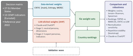
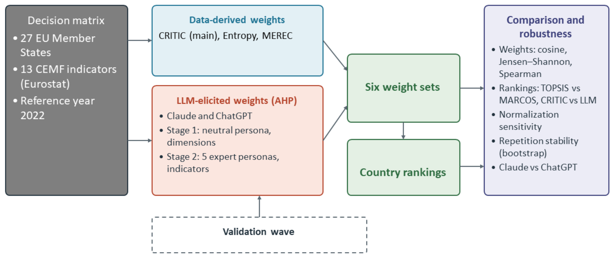
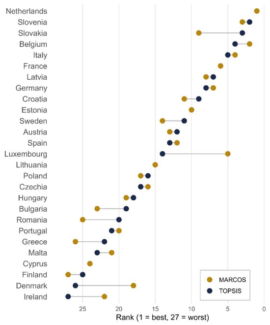
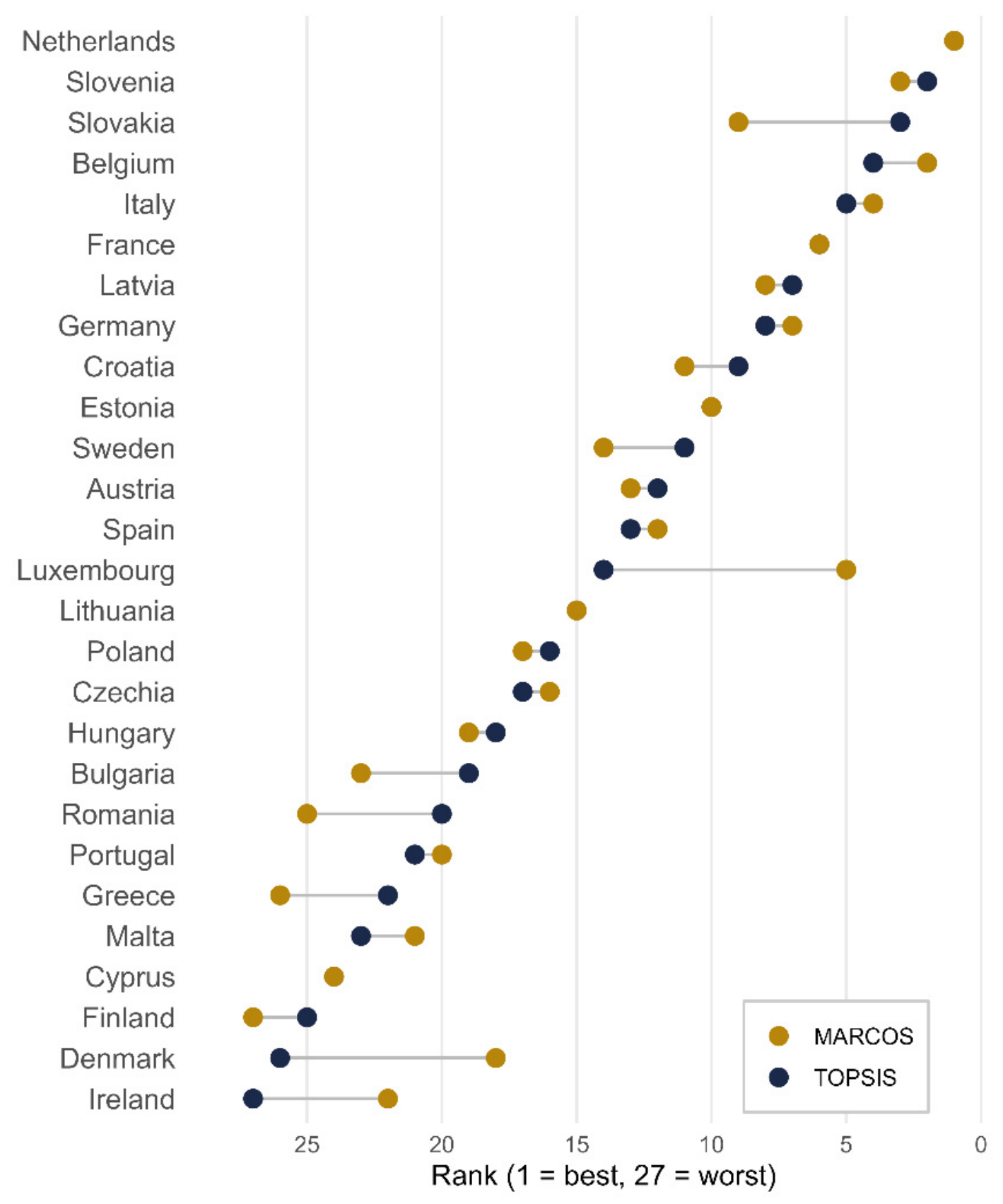
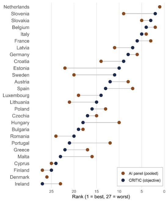
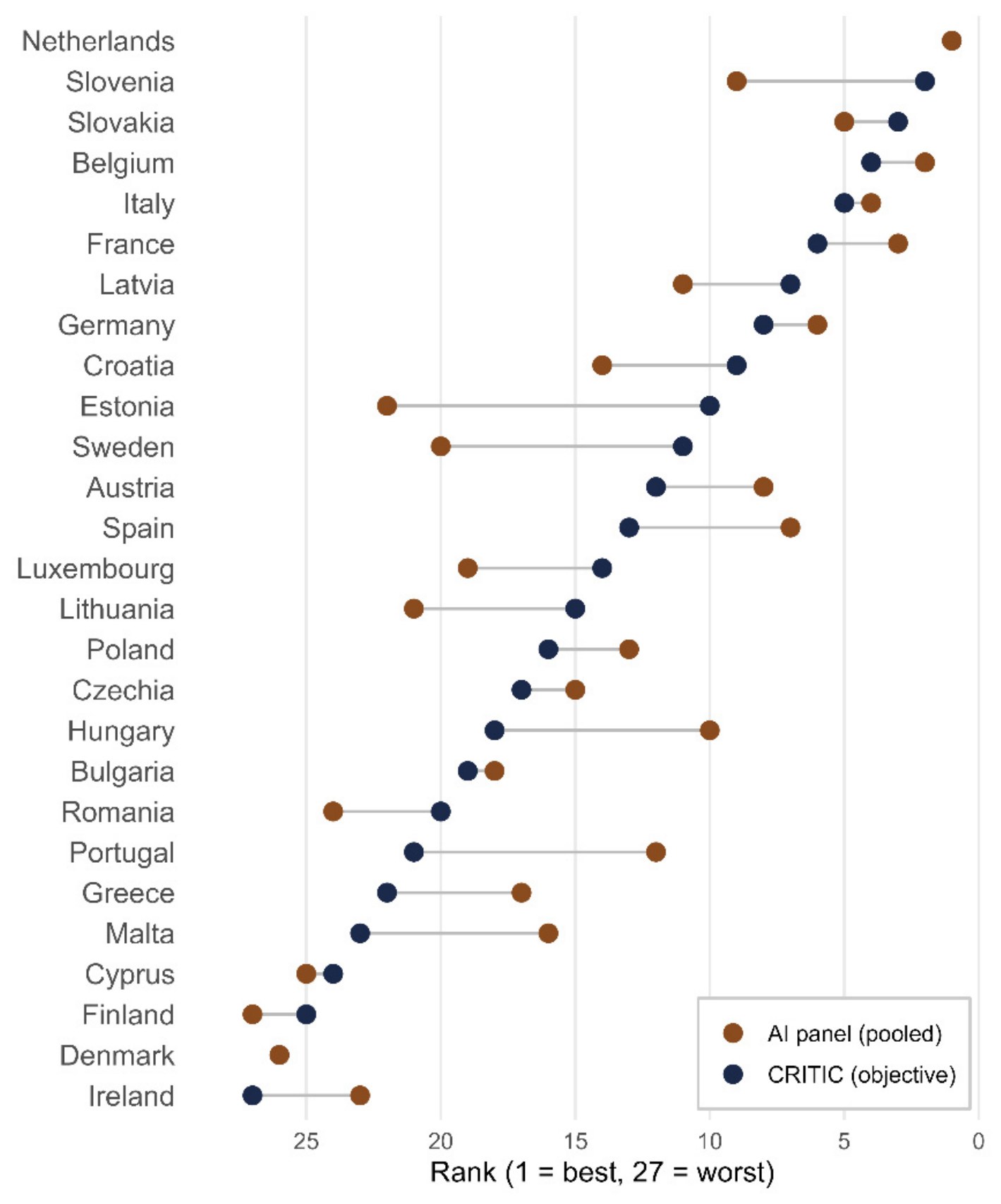

Disclaimer/Publisher’s Note: The statements, opinions and data contained in all publications are solely those of the individual author(s) and contributor(s) and not of MDPI and/or the editor(s). MDPI and/or the editor(s) disclaim responsibility for any injury to people or property resulting from any ideas, methods, instructions or products referred to in the content. |
© 2026 by the author. Licensee MDPI, Basel, Switzerland. This article is an open access article distributed under the terms and conditions of the Creative Commons Attribution (CC BY) license.