


Abstract
Cryptocurrency-energy assessments often conflate electricity use, emissions attribution and avoided system emissions. This targeted, non-exhaustive integrative review separates these quantities and evaluates mining-flexibility claims in European electricity systems. A six-criterion appraisal links principal studies to supported claims and transfer limits. A general electricity-accounting benchmark uses secondary data to compare 2024 production-mix and residual-mix direct CO2 factors for 24 national European Union domains. Their unweighted means are 214.38 and 415.18 g CO2/kWh; the median within-country ratio is 1.95. The two orderings have a Spearman correlation of 0.670 and disagree for 68 of 276 country pairs. The residual factor exceeds the production factor in all 24 countries in both 2024 and a matched 2025 comparison; consumption-weighted contrasts also remain positive. For a fixed hypothetical 1 MW Hungarian load operating throughout leap year 2024, the two accounting descriptors yield 1556.5 and 2798.9 tonnes of attributed direct CO2, a 79.82% accounting difference. These descriptive, non-causal results compare accounting descriptors, which are not freely interchangeable facility reporting options. Conditional procurement scenarios and an explicitly assumed four-hour example distinguish reported emissions, electricity volume and operating schedules. Technical evidence supports curtailment and ancillary-service participation in specified settings, but price responsiveness alone does not establish lower emissions. The applied framework links European disclosure to claim-specific counterfactuals and specifies requirements for joint assessment of heat, methane, water, hardware and health impacts.
1. Introduction
Bitcoin’s original design links permissionless consensus to computational work, whereas blockchain architectures more broadly encompass different trust assumptions and validation mechanisms. This distinction matters for sustainability research: the electricity demand of proof-of-work mining is not an intrinsic requirement of every distributed ledger or energy-market application. Technical accounts of Bitcoin, architectural comparisons and early sustainability assessments provide the basis for separating these objects of analysis [1,2,3,4].
The mining literature has moved from network-level electricity estimates towards geographically differentiated footprints, life-cycle assessment and grid-interactive operation. Reviews have consolidated evidence on hardware demand and environmental impacts, but their estimates refer to different periods, cryptocurrencies, functional units and system boundaries [5,6,7].
Comparison requires a clear distinction between facility electricity consumption, emissions attributed to that consumption and changes in electricity-system emissions caused by an intervention. Production-based indicators, flow-traced consumption accounting and residual-mix disclosure describe different relationships between electricity and emissions [8,9,10]. Marginal estimates instead concern emissions caused or avoided by a specified intervention [11,12].
The European setting also requires attention to contractual electricity attributes. The Markets in Crypto-Assets Regulation and the associated delegated sustainability-indicator regulation establish a disclosure context in which energy consumption and climate-related information have practical relevance [13,14]. Reporting compliance and causal environmental performance remain separate questions. A metric may be specified for disclosure without being an appropriate estimator of the emissions avoided by a particular dispatch decision.
The review addresses three research questions that connect the literature interpretation, quantitative accounting and the assessment of environmental claims.
- RQ1. What do published studies establish about cryptocurrency mining’s electricity use and environmental impacts, and which methodological differences limit comparison of their findings?
- RQ2. How do production-mix and residual-mix direct CO2 factors differ across 24 national European Union domains, and how sensitive are these differences to year, electricity-consumption weights and country coverage?
- RQ3. Which evidence and counterfactuals are required to assess operational and environmental claims about cryptocurrency mining in European electricity systems?
The contribution combines a critical synthesis of published evidence with a reproducible comparison of European accounting descriptors and an applied framework for mining claims. Established attributional and consequential assessment methods provide the methodological basis [9,10,11,12]. The accounting analysis quantifies how factor definitions affect attribution and country ordering, while the framework specifies the computational output, grid service or useful heat that an operational comparison must make explicit. Hungary provides a standardized fixed-load illustration without assuming an observed national mining fleet. The resulting contribution concerns evidence interpretation and study design; the national accounting data do not support a site-selection or investment model.
The analysis follows these questions in sequence. Section 3 synthesizes published findings and their limits of comparability (RQ1). Section 4 compares the national accounting descriptors and evaluates the stated sensitivities (RQ2). Section 5 uses these distinctions to appraise operational and environmental claims in Europe (RQ3), ending with a summary of the answers and contributions. Section 6 and Section 7 set out the remaining limitations, research priorities and conclusions.
2. Review Design and Quantitative Methods
2.1. Review Type and Evidence Identification
The study is a critical integrative review with an embedded secondary-data accounting analysis. Integrative methods are appropriate when a question combines theoretical arguments, engineering models, environmental inventories, observational information and institutional documents [15,16,17]. The three questions are addressed through targeted scholarly and institutional web searches, exact-title searches and backward citation tracing. Sources were consulted up to 26 October 2026. Supplementary Section S7 records the search themes, eligibility rules, access routes and selected exact source-verification queries. The synthesis is non-exhaustive and does not estimate a pooled effect of mining on emissions from studies with incompatible counterfactuals.
The bibliography identifies the sources used in the synthesis. The retained search record documents the routes used to verify principal studies and institutional material, but it does not support complete retrieval and exclusion counts or the first-identification route of every publication. Coverage refers to the stated research themes and assessed sources rather than all the eligible literature. Selection decisions and the limits of the detailed case appraisal are described below and in Supplementary Section S4.
Sources were retained when they addressed a defined technical mechanism, supplied an identifiable environmental or operational estimate, explained an accounting method, or established a relevant data or disclosure framework. Academic evidence was drawn from published journal articles and conference papers; unpublished research preprints were excluded. Original protocol documents, institutional reports, technical and accounting guidance, legal sources and identifiable operator disclosures were retained for their respective technical, methodological, implementation or reporting roles. Research on coupled electricity and resource systems was included where it clarified an assessment requirement, with its application to mining stated separately from the source findings. General cryptocurrency-price forecasting, unrelated blockchain applications and promotional assertions without an identifiable evidential basis were outside the analytical focus. Operator reports were eligible as evidence of reported implementation, but environmental-effect claims required the same inventory and counterfactual appraisal as academic studies. Legal sources were used to describe reporting requirements, not to infer environmental effectiveness. Searches did not use proprietary Scopus or Web of Science exports. No protocol was registered and no independent duplicate screening was conducted; exhaustive coverage and inter-rater agreement are not claimed.
Access depth varied across publications. The synthesis draws on accessible original full texts and institutional reports, supplemented by publisher or author-institution abstracts for specific findings. Abstract-level evidence is restricted to the information explicitly reported there; detailed methodological validation is not inferred from an abstract. Supplementary Table S4 applies the six appraisal criteria to a purposive set of principal sources and identifies the inspected material. A European commercial heat-recovery report is included to distinguish implementation evidence from independently verified environmental performance. Selection and availability bias remain limitations, particularly for unpublished operating data and commercially confidential European facilities.
2.2. Evidence Appraisal and Synthesis
The claim appraisal is organized around six questions: what is measured or modeled; which period and geography are covered; what physical and accounting boundaries apply; what counterfactual is specified; which assumptions and validation or uncertainty evidence condition the result; and what can be transferred to Europe? Supplementary Table S4 makes all six questions explicit for each selected source, including when a counterfactual is unnecessary for a descriptive claim or when evidence is insufficient for a stronger claim. This appraisal avoids a single numerical quality score that would place a laboratory measurement, a global inventory and a theoretical consensus model on an artificial common scale.
Three distinctions are structured in synthesis. First, an observation is separated from a model-derived estimate and a prospective scenario. Second, attributional accounting is separated from consequential system change. Third, a study’s setting is separated from the population to which an interpretation is extended. Industry-affiliated studies are neither discarded nor accepted on affiliation alone; their assumptions, data availability and type of validation determine their evidential use. The same scrutiny applies to critical commentaries and studies advocating particular interventions.
The review does not pool published TWh, tonnes of CO2-equivalent or monetary-damage estimates. They are not interchangeable effect sizes: annualized snapshots differ from calendar-year totals; CO2 differs from CO2-equivalent; and global network estimates differ from facility studies. Instead, selected estimates are retained with their original time and boundary labels. The quantitative contribution below is independently defined and does not treat the number of cited studies as a statistical sample of mining outcomes.
The nine detailed appraisals in Supplementary Table S4 span inventories, prospective scenarios, operational flexibility, heat recovery, methane, exposure, European electricity accounting and an operator-reported installation. These cases are retained for their direct relevance to the research questions and their complementary claim types, methods and access conditions; the same six questions are documented for each case. The five cases in Section 5.5 are a presentation subset that contrasts flexibility, heat, methane, exposure and European implementation claims; they are not an additional study sample. This is a worked application of the framework, not validation of a scoring instrument or an estimate of how frequently the wider literature satisfies the criteria.
2.3. European Accounting Dataset and Inclusion Rules
The principal accounting benchmark uses the Association of Issuing Bodies’ European residual mixes for calendar year 2024, version 1.1 dated 11 August 2025. Residual factors were extracted from Table 2 (Residual Mixes 2024) of the AIB report and production factors from Table 5 (Production Mix 2024) of that report, preserving the source’s direct CO2 units and two-decimal precision [18]. The same 24-country frame was also evaluated with the 2025 release, version 1.0 dated 26 May 2026, using the corrected values in Table 2 of that AIB report, including the explicit Italy correction, and the production factors in its Table 5 [19]. The 2024 cross-section provides the principal accounting benchmark, and the matched 2025 comparison tests whether the direction and magnitude of the contrasts recur in the subsequent available year. Each comparison pairs factors within one year and one identified release. Both vintages use the shifted issuing-based method, combining calendar-year production with GO transactions from 1 April of that year to 31 March of the following year. Changes in production, attribute activity and source-factor inputs remain combined in the annual comparison [18,19].
The starting frame comprises 27 EU-labeled domains. Austria and the Netherlands have no numerical residual factor in the selected table and are excluded from paired calculations rather than assigned zero. The Ireland domain covers the all-island system and is excluded from the strictly national EU comparison because its boundary includes Northern Ireland. This leaves 24 national domains in both years. A 2024 sensitivity analysis adds the all-island entry without relabelling it as a Republic-of-Ireland observation. Supplementary Table S1 retains the original inputs and exclusions; Table S5 gives the matched 2025 inputs and both years’ consumption weights.
Production and residual factors are compared as country-level accounting descriptors with different denominators and meanings, not as methods that a facility may freely select. A production factor describes domestic generation. For location-based reporting, GHG Protocol gives preference to regional or subnational grid-average factors that reflect net physical imports and exports; national production factors are a lower-tier option [10]. This benchmark does not assume that its national production column supplies the appropriate facility location-based factor. Market-based reporting instead follows the applicable hierarchy of qualifying contractual instruments, supplier information and residual information for uncovered consumption [9,10,18]. AIB’s national calculations become official disclosure factors when adopted by the relevant authority, so national implementation and the reporting year must be checked before facility use [18]. None of these attributional factors identifies the marginal generator or a complete life-cycle footprint. Table 1 distinguishes their analytical roles.
Table 1.
Quantities that must be distinguished in cryptocurrency-energy assessment.
2.4. Statistical Estimands and Calculations
Let and denote the production and residual direct CO2 factors for country , measured in g CO2/kWh. The accounting difference and ratio are defined in Equation (1):
All production factors in the included frame are positive, so the ratios are defined. These statistics describe changing the factor while holding electricity consumption constant; they do not describe a physical change in power generation.
For , , and , the analysis reports the unweighted arithmetic mean, median, first and third quartiles, interquartile range, population standard deviation and observed range. Quartiles use linear interpolation, equivalent to the type-7 convention. Population standard deviations use denominator because the analysis describes the complete included frame, not a random sample from an assumed superpopulation. The coefficient of variation is population standard deviation divided by the mean. Equal country weights answer a jurisdictional-comparison question; they do not estimate an electricity-weighted EU emission factor or a mining-weighted footprint.
The consumption-weight sensitivity uses each country’s total electricity consumption in Table 4 (Total Supplier Mix 2025) of the AIB report for the corresponding year. For each descriptor, the products of country consumption and its factor are summed and divided by the consumption sum; identical within-year weights are applied to production, residual and paired-difference values. Volumes are retained to the published two-decimal TWh precision. This asks whether larger electricity markets alter the descriptive contrast. It does not estimate a physical EU consumption factor, a mining footprint or an aggregate residual mix: the latter would require weights for untracked electricity, whereas a physical production aggregate would require generation weights and a consumption inventory would additionally require its own exchange treatment. AIB treats transmission and distribution losses as consumption within its disclosure calculation; these volumes are not presented as final end-use demand [18,24].
Spearman’s rank correlation measures correspondence between the two factor orderings. Kendall’s tau measures concordance across country pairs. The discordance condition and the number of distinct pairs are given in Equation (2):
Here and identify different countries, is the number of included countries, and is the number of distinct country pairs. There are no ties in the included values. The pairwise inversion fraction makes the practical meaning of the rank statistics explicit. The ordering statistics describe the emission factors, not overall environmental performance.
No null-hypothesis test is attached to these descriptive comparisons. Country factors are interdependent through electricity and attribute markets, and the included countries are not a probability sample. A small -value would not resolve either issue. Leave-one-country-out calculations are used as selection sensitivity checks, not as confidence intervals. A second sensitivity calculation incorporates the all-island Ireland domain. Rounding sensitivity considers the two-decimal precision of the reported inputs but does not represent uncertainty in the underlying inventories.
2.5. Standardized Hungary Illustration
For a facility-metered electrical load in MW and operating duration in hours, electricity use is measured in MWh. With an accounting factor in g CO2/kWh, attributed direct emissions are measured in tonnes CO2. Equation (3) applies the corresponding unit conversion:
The benchmark sets MW and h, the full duration of leap year 2024. It describes a hypothetical continuously operating facility, not a measured Hungarian mine. Because the load is defined at the facility meter, an additional power-usage-effectiveness multiplier would double-count auxiliary consumption. This is a general electricity-accounting benchmark whose calculations apply to any consumer with the same metered load and operating schedule. Mining hardware efficiency, hashrate, network difficulty and revenue are not modeled, so the benchmark does not estimate mining output or profitability.
The procurement extension holds electricity use, the operating schedule and national annual factors fixed, and varies the share covered by qualifying electricity attributes. Uncovered consumption is assigned the residual factor only where it is the applicable fallback after the contractual-instrument and supplier-data hierarchy [10,18]. Covered consumption is assumed to carry eligible wind or solar attributes with zero direct CO2; this is an explicit scenario assumption, not a claim that all renewable contracts have identical emissions. A separate four-hour illustration in Section 5.1 uses stated, assumed prices, marginal factors and load schedules to demonstrate timing and volume effects. It is not an observed European time series. The benchmark excludes direct on-site fuel combustion, upstream fuel emissions, equipment manufacture, construction, transmission losses outside the source factor boundary and non-CO2 gases. Its CO2 results must not be presented as complete Scope 1–3 or life-cycle CO2-equivalent inventories.
3. What the Cryptocurrency-Energy Literature Establishes
RQ1 concerns what the published evidence establishes and whether its findings describe comparable quantities. The synthesis first distinguishes consensus mechanisms and estimation methods, then examines emissions, flexible operation and coupled environmental effects. This ordering identifies the boundaries needed for the accounting comparison in Section 4 and the claim appraisal in Section 5.
3.1. Consensus Mechanisms and the Correct Comparison Unit
Proof-of-work mining expends computation in competition for block rewards and transaction fees. It should be distinguished from ordinary ledger storage and validation. Proof-of-stake models alter the consensus resource and incentive structure; their energy characteristics cannot be estimated by applying Bitcoin’s mining intensity to all blockchain transactions [25,26]. Ethereum’s transition provides evidence that a change in consensus architecture can substantially alter operational electricity requirements, although the consequences for other design objectives must be assessed separately [27].
Early multi-network studies also show why Bitcoin-only accounting should not be labeled a footprint of all cryptocurrencies. Zade et al. developed a scenario model covering more than one blockchain, while Gallersdörfer et al. compared the power demand of multiple cryptocurrencies before Ethereum’s consensus transition [28,29]. Their historical estimates remain informative about method and coverage, but their network composition is not a description of the post-transition ecosystem. The distinction extends to blockchain applications within the energy sector. Andoni et al. reviewed energy-sector implementations, and Mengelkamp et al. examined the design requirements of a microgrid market [30,31]. These studies concern coordination, market design and information exchange, not evidence that additional proof-of-work mining reduces electricity-system emissions. Wüst and Gervais show that the need for a blockchain depends on trust and application requirements [32]. A low-energy permissioned ledger may support electricity-attribute tracing without inheriting Bitcoin’s computational competition.
This separation prevents two symmetric errors. One is to dismiss every blockchain-enabled energy application using Bitcoin’s electricity demand. The other is to use the possible benefits of an energy-trading platform to justify the footprint of an unrelated mining network. The relevant comparison is between alternative systems delivering a specified function with stated security, governance and performance requirements. An electricity-per-transaction ratio rarely supplies that comparison [2,4].
3.2. Network Electricity Estimates: Hardware, Economics and Time
Engineering estimates generally combine network hashrate with assumptions about the active hardware fleet and facility overhead. Economic approaches infer feasible expenditure or operating decisions from mining revenues and electricity costs. Both require information that is incompletely observed. De Vries’ early and subsequent analyses emphasize the relevance of equipment economics, hardware-market constraints and changing incentives [33,34,35]. These approaches do not produce a universally observable network electricity meter.
Küfeoğlu and Özkuran’s review of hardware and demand illustrates how equipment assumptions generate materially different estimates for a common period. Stoll et al. linked hardware information and mining geography to an annualized electricity and emissions estimate, while Köhler and Pizzol constructed a life-cycle inventory for a defined calendar year [5,20,36]. Table 2 preserves these distinctions rather than treating the published values as independent measurements suitable for averaging.
Table 2.
Selected published estimates, retained with their original scope rather than pooled.
The 2025 Cambridge industry report adds operator information from 49 firms covering about 48% of network hashrate at collection. It estimates annual electricity consumption at 138 TWh and reports emissions estimates of 39.8 Mt CO2e from its survey-based approach versus 69.6 Mt CO2e from an IP-based approach [38]. These are different model results, not lower and upper bounds of a statistical confidence interval. Extensive hashrate coverage does not by itself remove geographic or participation bias.
The Cambridge index’s methodological notes distinguish daily power estimates, monthly accumulation and annualized quantities [41]. This distinction is essential when comparing a rapidly changing network across papers. Multiplying the power estimated on a particular day by the hours in a year creates an annualized operating rate; integrating changing power estimates over a year creates a calendar-year energy estimate. Their numerical difference is not automatically disagreement about the same quantity.
Official U.S. work also demonstrates the limits of capacity-based inference. The Energy Information Administration’s 2024 analysis combined top-down and bottom-up approaches and explicitly noted incomplete knowledge of facility operation [39]. Announced connection capacity, installed capacity and metered average demand are different variables. Transferring such estimates to Europe using population, GDP or an assumed share of global hashrate would add unsupported assumptions rather than resolve the underlying data gap.
3.3. Carbon Inventories and Contested Extrapolations
The carbon intensity of mining depends on where electricity is generated, when it is consumed and what inventory boundary is chosen. Krause and Tolaymat compared energy and carbon costs across cryptocurrencies using a monetary functional unit; Köhler and Pizzol assessed life-cycle contributions; and de Vries et al. revisited the role of mining geography in the carbon footprint [20,42,43]. A monetary denominator changes with market prices even when the physical process is unchanged. A life-cycle denominator adds processes not contained in direct power-generation CO2.
The debate following Mora et al.’s warming projection provides a methodological lesson. Masanet et al., Houy, and Dittmar and Praktiknjo challenged assumptions concerning extrapolation, economic viability and the connection between transactions and electricity demand [44,45,46,47]. The disagreement does not make environmental assessment unnecessary. It shows that a global temperature trajectory cannot be inferred by mechanically scaling a static electricity-per-transaction ratio with adoption.
Scenario projections require similarly explicit labels. Jiang et al.’s model projected a 2024 peak under specified assumptions about Bitcoin operation in China [37]. That result is not an observed 2024 inventory and should not be plotted as a measured continuation of historical demand. A retrospective review must preserve the difference between what a model projected and what a later data source estimates, especially when the geographic distribution and operating environment changed.
Cross-border accounting adds another layer. Onat et al. examine direct and supply-chain footprints across countries, while Chamanara et al. extend analysis across carbon, water and land [48,49]. These approaches show that a low domestic generation factor cannot identify every environmental burden associated with equipment, fuel supply and operations. They do not remove the need to verify the location and characteristics of the mining fleet used in the inventory.
3.4. Price Responsiveness and Power-System Flexibility
Technical studies distinguish mining that operates continuously from mining that changes load in response to market or system signals. Menati et al. combine observed load–price associations with synthetic-grid simulations; the observed associations do not distinguish mandatory demand response from voluntary price response [50]. The presence of real market inputs does not turn all outputs of these studies into measured field effects. Menati et al.’s published conference study represents heterogeneous mining devices and the opportunity cost of ancillary-service participation, reporting simulated profit improvements using historical ERCOT traces [40]. This supports the feasibility of a specified dispatch strategy under the model’s assumptions. It does not establish that every participating facility improves system-wide emissions, or that the same settlement and qualification conditions apply in a European balancing market.
Related electricity–water research illustrates how coupled resource dynamics can be represented in operational optimization: Hua et al. develop a progressive polyhedral approximation for nonlinear electricity–water dispatch [51]. Its relevance here is methodological: a mining application would need to represent the facility’s own electricity, cooling and water constraints before an optimized schedule could be interpreted as feasible operation.
European evidence is emerging but requires the same separation. Pavlík and Bereš analyze flexible and continuous operation using French hourly prices for 2015–2025 and fixed technological parameters [52]. Their work is relevant to price-threshold modeling; it does not provide a measured EU-wide mining inventory or establish a causal emissions benefit. A fixed technological representation over a long period is a scenario assumption, not a reconstruction of changing fleets, difficulty and network rewards.
The Cambridge survey reports 888 GWh of curtailed load in 2023 among responding miners [38]. This is evidence of reported operational curtailment, not an estimate of avoided emissions. It cannot be divided by a later global annual-demand estimate to construct a valid global curtailment share. Nor does compensation for turning down an existing load show that adding that load was beneficial relative to a system without it. A curtailable mine is also not an electricity storage device. Reducing demand can release capacity to other users, but the mining equipment does not subsequently return stored electricity to the grid. Moreover, curtailed computation is not necessarily a deferrable job that can be completed later with equivalent economic output: mining is a time-dependent competition. Comparisons with storage accordingly require a common service definition, including response time, duration, availability and whether the asset supplies energy or only reduces consumption.
3.5. Heat Recovery and Methane-Based Electricity
Heat recovery changes the system boundary from electricity consumption alone to a combined mining-and-heat service. Chen and You examine greenhouse integration through model predictive control across different climatic settings [53]. The relevant environmental comparison is between two ways of delivering the same useful heat and other specified outputs, not between a mine with an acknowledged heat stream and an imaginary mine with no electricity input. A defensible avoided-heat claim requires measured useful heat, its temperature, seasonal demand, distribution losses, auxiliary electricity and the technology actually displaced. Heat rejected during periods without a customer has no avoided-heating benefit. Substituting recovered heat for resistance heating, a heat pump or an existing waste-heat source produces different consequences. These are derived requirements for the comparison; the review does not assign a generic avoided-emissions credit to every unit of mining electricity.
Rudd et al. develop a landfill-gas-to-energy and Bitcoin-mining framework [54]. Its mitigation mechanism depends on the treatment of methane that would occur without the project. The appropriate baseline may be uncontrolled release, flaring, existing electricity generation or another gas-use pathway. Destruction efficiency, leakage, methane slip and the chosen climate metric can change the result. An electricity revenue stream and a methane-control benefit are analytically distinct, even when they occur within one project.
Research-agenda work also identifies questions raised by industry participants [55]. Such material can guide hypothesis development and reveal operational constraints, but it is not a substitute for an independently specified baseline and measured flows. Neither commercial involvement nor a critical stance determines whether a particular estimate is correct. Verifiable inputs and the treatment of alternatives remain the relevant tests.
A European implementation example is MARA’s June 2024 report of a 2 MW mining installation integrated with district heating in Finland’s Satakunta region [56]. The operator account identifies an installation and heat-delivery arrangement, but it does not provide the synchronized annual electricity and useful-heat records, displaced-plant operation and independently evaluated counterfactual required here for a net avoided-emissions estimate. It is retained as operator-reported implementation evidence. Supplementary Table S4 and the worked application in Section 5.5 show how the framework permits this limited claim without endorsing the report’s broader environmental assertions.
3.6. Environmental and Health Impacts Beyond Operational CO2
Electronic waste, cooling demand and upstream resource use prevent a complete sustainability assessment from being reduced to one electricity factor. De Vries and Stoll model hardware obsolescence and e-waste, while the broader assessment by de Vries et al. discusses impacts beyond energy use [21,57]. Longer service life can reduce replacement-related burdens, but equipment export, reuse and final disposal need separate treatment. A reused machine is not necessarily absent from the global electricity system.
Water accounting similarly requires distinctions between on-site cooling and water associated with electricity supply. De Vries’ water-footprint analysis and the multi-impact work of Sial et al. illustrate these additional boundaries [22,58]. Water withdrawal, consumption and scarcity-weighted impact are not equivalent quantities. The same volume can have different implications across locations and seasons. The present CO2 benchmark cannot resolve these dimensions and is not used as their proxy.
Health-related evidence is relevant to the distribution of impacts. Goodkind et al. estimate monetary damages from air pollution and health effects; Guidi et al. model pollution associated with large U.S. Bitcoin facilities; and Willis et al. discuss potential health hazards [23,59,60]. These sources represent different evidence types, including model-based exposure assessment and a clinical-journal viewpoint. They do not constitute an observed epidemiological effect of Hungarian mining. European extrapolation would require plant-level emissions, atmospheric transport, population exposure and locally appropriate concentration-response relationships.
Jones et al.’s climate-damage valuation also depends on the damage factor applied to emissions and on the monetary denominator [61]. Damage-to-price or damage-to-revenue ratios should accordingly be reported alongside physical quantities, valuation assumptions and the relevant period. Changing the valuation coefficient is not a measured change in emissions. Keeping these layers separate allows sustainability claims to be examined without collapsing environmental, health and financial outcomes into a single ambiguous score.
4. European Quantitative Accounting Results
RQ2 isolates a specific comparability problem: the same electricity volume can receive different direct CO2 attributions under production and residual descriptors. The analysis first reports country distributions and orderings, then illustrates the consequences for a fixed hypothetical Hungarian load and procurement assumptions, and finally tests geographic, annual and weighting sensitivities. These calculations describe accounting differences without estimating the physical emissions effects of mining.
4.1. Distribution of Production and Residual Factors
Across the 24 included national domains, the unweighted mean production factor is 214.38 g CO2/kWh and the mean residual factor is 415.18 g CO2/kWh. Their medians are 194.71 and 413.74 g CO2/kWh. The median paired difference is 182.91 g CO2/kWh, with an interquartile range of 285.91 g CO2/kWh. The residual factor exceeds the production factor in every included country. Table 3 reports the complete set of descriptive statistics, calculated from the fixed-year inputs.
Table 3.
Descriptive statistics for 24 national EU domains, 2024.
Production factors have a population standard deviation of 173.89 g CO2/kWh, compared with 190.69 g CO2/kWh for residual factors. Relative dispersion is smaller for residual factors: coefficients of variation are 0.811 and 0.459, respectively. This does not mean the residual accounting system is less uncertain. The coefficient describes cross-country dispersion relative to the cross-country mean, not precision of the original estimates or the validity of either boundary.
The paired comparison in Figure 1 shows that a single uplift applied to all production factors would not reproduce the residual factors. The mean paired difference is 200.80 g CO2/kWh, but the observed differences range from 5.45 to 458.46 g CO2/kWh. These absolute differences are the primary comparison for a common electricity volume: a difference of 1 g CO2/kWh corresponds to 1 tonne CO2 per GWh. They remain interpretable when a production denominator is close to zero, although they still describe attribution and do not establish which reporting factor is applicable to a facility.
Figure 1.
Production-mix and residual-mix direct CO2 factors for 24 national EU domains in 2024. Note: Countries are ordered by the production factor. The connecting lines indicate paired accounting descriptors, not changes in physical emissions. Austria, the Netherlands and the all-island Ireland domain are excluded from the main frame. Source: authors’ calculations from AIB [18].
4.2. Relative Differences and Ordering Changes
The median country-level ratio is 1.95, with an interquartile interval of 1.27–3.75. Twelve ratios exceed two and four exceed five. The mean ratio, 3.81, is substantially above the median because very small production factors produce large relative differences. Ratios are retained as a secondary proportional descriptor; the median and interquartile interval accompany the absolute differences to prevent a few low denominators from dominating interpretation. The ratio of the two means, 1.937, answers a different question from the mean of country ratios, 3.808.
Sweden, Finland, Portugal and Denmark have ratios of 16.93, 12.22, 11.59 and 8.24, respectively. These describe the relative separation of two accounting factors. They do not mean that residual accounting causes physical emissions to multiply by those amounts. Sweden’s 80.47 g CO2/kWh absolute difference is smaller than Hungary’s 141.44 and Portugal’s 458.46, despite Sweden having the largest ratio. Its production factor of 5.05 g CO2/kWh explains the large proportional value, while its residual factor remains the second lowest in the 24-country frame.
The correspondence between factor orderings is positive but incomplete: Spearman’s correlation is 0.6696 and Kendall’s tau is 0.5072. Of 276 distinct country pairs, 68 are in reverse order, giving an inversion fraction of 24.64%. Figure 2 displays the underlying paired values rather than a fitted causal model. Countries above the identity line have higher residuals than production factors; dispersion around a hypothetical regression line would not identify the cause of the difference.
Figure 2.
Correspondence between production and residual factors, 2024. Note: The dashed line denotes equal factors, not a fitted regression. Spearman and Kendall ; 68 of 276 country pairs are in reverse order. Country codes are defined in Supplementary Table S1. Source: authors’ calculations from AIB [18].
Selected contrasts in Table 4 combine absolute differences, ratios and ascending factor ranks. Portugal moves from rank 4 under production to rank 16 under residual accounting, Finland from 3 to 12, Lithuania from 10 to 18 and Denmark from 6 to 13. Romania and Malta each move nine places in the opposite direction, while Hungary moves from 12 to 7. These changes show that country ordering depends on which accounting construct is compared; they do not represent changes in the physical performance of those electricity systems. Figure 3 presents all ratios on a logarithmic axis.
Table 4.
Selected absolute differences and changes in ascending factor ranks in 2024.
Figure 3.
Residual-to-production factor ratios for the 24-country frame. Note: The horizontal axis is logarithmic. Large ratios can arise from small production-factor denominators and do not imply a physical increase in emissions. Source: authors’ calculations from AIB [18].
The country mechanisms are consistent with the way electricity attributes are removed and reallocated, but the paired factors alone cannot isolate the contribution of each mechanism. AIB’s 2024 production mixes contain renewable shares of 70.32% in Sweden, 55.98% in Finland, 89.20% in Portugal and 90.41% in Denmark; nuclear generation further lowers direct production intensity in Sweden and Finland. Their residual renewable shares are 50.70%, 11.25%, 4.13% and 24.45%, respectively [18]. Domestic low-carbon generation and the attributes available to an untracked purchaser can thus differ substantially. These source shares are an accounting composition, not a reconstruction of the electricity physically delivered to each end user.
Finland, Denmark and Portugal require 13.87, 13.98 and 36.61 TWh of European Attribute Mix contributions to balance their 2024 residual attributes, whereas Sweden contributes a 1.79 TWh surplus [18]. The deficits can reflect attribute issuance and expiry, cancelation and international attribute transfers, together with the production–consumption balance; they must not be interpreted as physical electricity imports or certificate exports alone. AIB’s total supplier mix combines canceled attributes and the residual allocation, whereas flow-traced consumption accounting follows electricity exchanges. These are distinct constructs [9,18]. Sweden also illustrates implementation limits: the Swedish authority’s contribution to AIB’s 2024 annual report describes a Nordic residual mix in national disclosure practice [62]. The harmonized Swedish value compared here is not automatically a facility’s nationally applicable default. Procurement assessments must verify the relevant authority’s factor, eligible contract and cancelation record.
4.3. Hungary Accounting Sensitivity and Procurement Scenarios
Hungary’s production and residual factors are 177.20 and 318.64 g CO2/kWh. The paired difference is 141.44 g CO2/kWh and the ratio is 1.7982. Applying the two descriptors to the same hypothetical 1 MW facility operating for all 8784 h gives 8.784 GWh of electricity use and attributed direct CO2 of 1556.5 and 2798.9 tonnes. This accounting-descriptor comparison gives a difference of 1242.4 tonnes, or 79.82% relative to the production descriptor, under the same fixed hypothetical load. The production-based number is a comparator, not an asserted location-based consumption inventory for that facility.
The facility has not changed equipment, output, location or operating hours in this calculation. The result isolates the effect of applying different descriptors to a common electricity volume. It cannot be interpreted as emissions caused by certificate markets, savings from low-carbon procurement or a measurement of Hungarian cryptocurrency mining. The reporting relevance depends on which factor is admissible under the actual electricity supply and accounting rules.
Table 5 extends the illustration to four stated procurement arrangements. All cases retain 8784 MWh, the production descriptor of 177.20 g CO2/kWh and the national residual factor of 318.64 g CO2/kWh. Only the covered fraction and resulting conditional market-based direct CO2 attribution vary. The assumed covered source has zero direct CO2 and qualifying attributes are owned and canceled for the reporting entity, period and eligible market. A bundled power-purchase agreement qualifies only if the environmental attributes are retained and satisfy the same applicable criteria [10].
Table 5.
Conditional procurement cases for the Hungarian illustration.
At 50% eligible coverage, 4392 MWh remains assigned to the residual factor, giving a combined reporting factor of 159.32 g CO2/kWh and 1399.5 tonnes of attributed direct CO2. Both fully covered arrangements yield zero within the stipulated direct-CO2 boundary, although their financing, additionality and dispatch consequences can differ. None of these results measures avoided system emissions. One buyer’s hypothetical procurement does not recalculate the national production or residual factors; modeling market-wide certificate supply, cancelation and investment responses would require an additional market model. For GHG Protocol inventories in markets with contractual instruments, location-based and market-based Scope 2 totals must both be reported; the location-based total is calculated separately using the appropriate grid factor and is not reduced simply by increasing certificate coverage [10].
A regional comparison also demonstrates why the applicable reporting boundary matters. Hungary’s production factor is 78.07 g CO2/kWh above Slovakia’s, but its residual factor is 15.69 g CO2/kWh below Slovakia’s. An assessment of otherwise comparable untracked purchases can reverse the ordering obtained from domestic generation alone. Czechia and Poland have substantially higher factors under both descriptors in this 2024 frame [18]. Such comparisons identify the need to inspect contracts and grid-consumption boundaries; they do not establish the emissions effect of relocating mining capacity.
4.4. Sensitivity to Coverage and Input Precision
Including the all-island Ireland domain produces a 25-domain sensitivity frame. The mean paired difference becomes 197.57 g CO2/kWh, the median ratio becomes 1.88 and Spearman’s correlation becomes 0.6438. The inversion fraction becomes 77/300, or 25.67%. These values are close to the principal descriptive pattern, while the geographic distinction remains important for correct labeling.
In the 24 leave-one-country-out calculations, Spearman’s correlation ranges from 0.6245 to 0.7292 and Kendall’s tau from 0.4625 to 0.5573. The median difference ranges from 174.27 to 191.54 g CO2/kWh and the median ratio from 1.88 to 2.02. The result is not driven by a single country, but these intervals do not measure sampling uncertainty. They quantify how selected summaries change when one member of the analytical frame is removed.
Input rounding is a much smaller numerical issue than boundary choice. Allowing each reported factor to vary by 0.005 g CO2/kWh changes the mean paired difference by at most 0.01 g CO2/kWh. Hungary’s ratio lies between 1.79812 and 1.79827 under these rounding limits. This check addresses numerical precision only; unmeasured, methodological or temporal uncertainty in the source factors can be much larger. Table 6 keeps these forms of sensitivity separate. AIB states that its residual-mix calculation does not consider uncertainty in the emission factors [24]. Source-factor errors or revisions could alter close country orderings and ratios, particularly where production factors are small; no probability is assigned to those changes here.
Table 6.
Sensitivity to geographic inclusion and omission of one country.
4.5. Sensitivity to Year and Electricity Consumption Weights
The same 24 countries have numerical production and residual factors in the 2025 release. Table 7 reports a matched comparison, preserving within-year factor pairing and the original exclusions. It also compares equal-country summaries with common consumption-weight summaries using AIB’s total electricity consumption for each year [18,19].
Table 7.
Matched annual comparison and consumption-weight sensitivity.
The residual factor exceeds the production factor in every included country in both years. The unweighted mean paired difference rises from 200.80 to 208.86 g CO2/kWh, while the median ratio rises from 1.950 to 2.274. Ordering disagreement increases from 68 to 79 of the 276 country pairs. The direction of the paired contrast recurs in the second year, but two observations do not establish a long-run trend or stable country rankings. Hungary illustrates this qualification: its production factor falls to 140.86 g CO2/kWh in 2025 while its residual factor rises to 453.50, giving a ratio of 3.220 [19].
Using the corresponding year’s consumption weights for both descriptors, the 2024 production and residual values are 193.77 and 388.05 g CO2/kWh, giving a difference of 194.28. The corresponding 2025 values are 187.98, 375.75 and 187.77. Thus, the contrast remains positive after larger electricity markets receive greater weight, but its weighted magnitude declines while the unweighted mean difference rises. Country size affects the summary and the apparent year-to-year direction of the mean gap. The ratio of weighted means is 2.003 in 2024 and 1.999 in 2025; it is not the weighted mean of country ratios. These checks support the presence of accounting separation without turning the compared descriptors into EU emissions inventories.
5. Interpreting Flexibility and Environmental Claims in Europe
RQ3 asks what additional evidence is needed to move from electricity quantities and accounting descriptors to claims about operation or environmental effects. The analysis proceeds from operating schedules and counterfactuals to procurement, facility data, source appraisal and interactions among environmental outcomes. The national benchmark supplies an accounting comparison; it does not empirically test flexible operation or net environmental benefits.
5.1. Annual Accounting Is Not a Dispatch Model
The quantitative benchmark establishes sensitivity to factor definition, not a causal relationship between mining and electricity-system emissions. A production factor averages generation within a boundary. Flow-traced consumption accounting includes a representation of cross-border electricity exchange [9]. Residual accounting concerns unclaimed attributes after explicit tracking. A marginal factor concerns the change in emissions associated with a change in demand. Replacing one with another changes the question being answered. This distinction is supported by the wider electricity literature. Hawkes separates short-run and long-run marginal effects; Siler-Evans et al. demonstrate differences between average and marginal factors; and Graff Zivin et al. examine temporal and spatial heterogeneity [11,12,63,64]. Their numerical estimates concern their own systems and periods, not present-day Hungary. The transferable contribution is the analytical requirement to match the emission factor to the intervention and time horizon.
For time intervals with duration in hours, facility load in MW, electricity price in EUR/MWh and an appropriate marginal factor in tonnes CO2/MWh, electricity use in MWh, operating electricity cost in EUR and the first-order emissions approximation in tonnes CO2 are given by Equations (4)–(6):
For a small load change , the corresponding first-order change is approximated by Equation (7):
Large mining additions can themselves change dispatch and capacity, so fixed marginal factors may then be insufficient. With equal-duration intervals, Equation (8) separates the product of the mean load and mean marginal factor from their covariance:
The overbar denotes an arithmetic mean across intervals and is the population covariance across the same intervals. Price-responsive operation determines the relationship between load and prices; it does not, by itself, determine . Lower prices and lower marginal emissions can coincide, but this is an empirical property of the relevant market and period, not an identity. Negative or low prices are a candidate scheduling signal, not proof that electricity consumption has zero incremental emissions.
Figure 4 provides a numerical illustration using four one-hour intervals, a 1 MW facility limit, assumed electricity prices of 20, 40, 60 and 80 EUR/MWh, and assumed marginal factors of 0.8, 0.6, 0.1 and 0.3 tonnes CO2/MWh. The uniform, price-led and emissions-led schedules each consume 2 MWh, while a fourth schedule deliberately reduces consumption to 1 MWh. All inputs are constructed for the illustration and are reproduced in Supplementary Tables S6b–S6d; none is an observed Hungarian or other European market series.
Figure 4.
Assumed operating schedules and their electricity-cost and first-order emissions consequences. Note: Left: load in four one-hour intervals. Right: total electricity cost and emissions under the fixed assumed marginal factors. The uniform, price-led and emissions-led schedules each consume 2 MWh; the reduced-volume case consumes 1 MWh. In panel (a), cell shading denotes load: very light gray = 0 MW, light blue = 0.5 MW and dark blue = 1 MW. In panel (b), blue, orange and green circles identify the uniform baseline, price-led and emissions-led schedules, respectively; the gray square identifies the reduced-volume schedule. Circles denote the three 2 MWh schedules and the square denotes the 1 MWh schedule. All prices, marginal factors and schedules are constructed; the diagram contains no observed market data. Inputs and calculations are given in Supplementary Tables S6b–S6d.
At equal electricity use, the price-led schedule costs EUR 60 instead of EUR 100 but raises the first-order emissions approximation from 0.9 to 1.4 tonnes. The emissions-led schedule gives 0.4 tonnes at EUR 140. For the price-led case, the load–price covariance is negative while the load–marginal-emissions covariance is positive; the latter is 0.125 in the units implied by Equation (8). This verifies the logical possibility of a lower-cost schedule with higher marginal emissions. It does not estimate its frequency, size or economic feasibility in Europe, and equal energy is not assumed to imply equal rewards or revenue. The profiles are chosen as a counterexample to a necessary link between lower prices and lower emissions. If the cheapest intervals also have the lowest marginal factors, the price-led and emissions-led schedules can coincide; with constant marginal factors, equal-energy schedules have equal emissions within the example’s fixed-factor boundary.
The annual benchmark does not identify an optimal schedule. ENTSO-E’s public data catalog provides load, generation, electricity prices, physical flows and balancing information, but it does not identify a ready-made marginal CO2 time series among those data items [65,66]. Estimating marginal emissions from these inputs requires a separate, documented emissions or dispatch model; generation-average or flow-traced consumption intensities cannot be relabelled as marginal factors. European applications also need synchronized facility load, the relevant bidding zone or connection point, and treatment of transmission limits, storage, imports and forecast error [9,11,67]. The constructed example demonstrates the equations without claiming that these missing empirical inputs have been supplied.
5.2. Separate the Counterfactuals Before Claiming a Benefit
Four comparisons should not be conflated: reducing the operation of an existing mine; shifting a fixed electricity volume across hours; adding a flexible mine instead of an inflexible mine; and adding a flexible mine to a system that otherwise has no mine. The first can reduce consumption, the second changes timing, the third changes the characteristics of an additional load, and the fourth changes total demand. A beneficial result for one comparison does not establish the same result for the others.
A useful decomposition makes this explicit. Let and be electricity use under a baseline and alternative schedule, and let and be their load-weighted emission intensities under a common emissions framework. With and , Equation (9) decomposes the emissions difference:
The subscripts and denote the baseline and alternative, respectively. The first term is the electricity-volume effect and the second is the intensity effect. This exact accounting identity does not, on its own, establish a causal model, but it prevents lower total operation from being mislabelled as cleaner timing.
The reduced-volume schedule in Figure 4 has an intensity of 0.80 tonnes CO2/MWh, above the uniform baseline’s 0.45, yet its total falls from 0.9 to 0.8 tonnes because it consumes half as much electricity. Equation (9) allocates this difference to a −0.45 tonne volume effect and a +0.35 tonne intensity effect. Lower total emissions in this illustration accompany less activity and less favorable timing. This calculation prevents reduced operation from being interpreted as improved load-weighted intensity.
The output constraint also matters. Equal electricity use, equal hashes, equal expected block reward and equal revenue are not equivalent benchmarks. Hardware efficiency can change the relationship between electricity and hashes; difficulty and competing hashrate change the relationship between hashes and expected rewards; prices change revenue. A comparison should state which quantity is held constant and report any sacrifice of output. Otherwise, an apparent efficiency gain may simply reflect less activity or a different monetary denominator.
Financial evaluation must also retain the actual electricity tariff, equipment characteristics and opportunity cost of interrupted mining [40,52]. These parameters connect the chosen output constraint to the operating comparison and must be specified for the European market being assessed.
For grid services, the comparison should additionally identify the service provided and the alternative resource. Fast response by a mine may be technically useful without showing that it is the least-cost or lowest-emission source of that service. Availability during scarcity, verified baseline load, minimum duration, rebound behavior, reserve headroom and network location can all matter. The published Texas studies motivate such questions; they do not answer them for all European balancing areas [40,50].
Table 8 separates the operational mechanisms that can be transferred from ERCOT studies from the parameters that require European validation. ENTSO-E documents national differences in balancing-service-provider and balancing-responsible-party arrangements, while Fingrid’s participation guidance and aFRR product information illustrate product-specific technical requirements and qualification procedures [68,69,70]. These sources support conditional transfer of the modeling structure, not transfer of simulated ERCOT profit or emissions percentages.
Table 8.
Transfer of mining-flexibility methods to European electricity systems.
Finland’s automatic Frequency Restoration Reserve (aFRR) illustrates four separate requirements. Fingrid specifies a minimum bid of 1 MW and full activation within five minutes [70]; reserve resources may be aggregated, but the unit must satisfy product-specific prequalification and establish real-time telemetry before the test [69]. The bid threshold does not mean that a 1 MW mine can deliver 1 MW of reserve. Technical capability requires verified response to the control signal; market eligibility additionally requires the relevant provider and settlement arrangements. Profitability depends on reserve payments, electricity costs, forgone mining revenue and participation costs. Environmental effectiveness requires a separate comparison of the generation or reserve service displaced. This institutional example identifies the evidence required to assess a mine and does not establish observed participation or an emissions benefit.
European validation should specify the actual tariff and service product, verify metered response against an admissible baseline, and represent available cross-zonal capacity or local congestion. A common low price across a bidding zone does not prove that an individual connection can absorb otherwise curtailed generation. Heating obligations can also restrict curtailment: backup heat, thermal storage or loss of delivered heat must enter the comparison when mining is coupled to a heat customer [53,67].
5.3. Procurement, Additionality and Double Counting
The GHG Protocol’s 2015 Scope 2 Guidance distinguishes location-based and market-based accounting and sets quality criteria for contractual instruments [10]. A reported procurement claim and a physically induced change in generation are different forms of evidence. Brander et al. critically examine this distinction, while Bjørn et al. analyze how certificate-based claims can affect reported progress against corporate targets [71,72]. Their arguments concern the relationship between accounting and mitigation; they do not establish that every procurement arrangement has the same effect. De Vries’ analysis of renewable electricity and Bitcoin similarly separates renewable supply from the wider sustainability question [73].
For mining, a claim of low-carbon electricity should identify the generation source, ownership and retirement of attributes, temporal matching and whether the electricity would otherwise serve another user. A claim that procurement caused additional low-carbon generation needs a separate investment or system counterfactual. A residual factor is useful for interpreting untracked electricity, but it is not a universal substitute for supplier-specific information and does not reveal the additionality of a contract.
Evidence from another flexible electricity-intensive activity illustrates the importance of this distinction without providing mining-specific effect sizes. Ricks et al. model hydrogen production and show how temporal matching, deliverability and additional clean generation affect emissions under their U.S. scenarios [74]. The transferable questions concern matching and system change; the study’s numerical results cannot be assigned to Bitcoin facilities. Differences in product storage, operational constraints and willingness to interrupt prevent a simple one-to-one analogy.
Digital traceability can improve the recording and verification of attributes, but it cannot create physical additionality by itself. Babel et al. propose privacy-preserving emission tracing with shielded tokens [75]. Such architectures may help preserve information and avoid conflicting claims when the underlying inputs are credible. A blockchain record, however, does not independently establish the accuracy of a meter, the correct counterfactual or the emissions of a marginal power plant. Data integrity and environmental causality are complementary requirements, not substitutes.
5.4. Regional Interpretation and Facility-Data Requirements
The EU benchmark is regional in a specific and limited sense: it compares country-level electricity-accounting factors relevant to a common hypothetical load. It does not identify the location, size or energy procurement of the European mining industry. Global surveys and IP-based geography can provide context, but allocating them to individual EU countries requires explicit evidence. Headquarters, server endpoints, mining pools, hosting companies and physical machines need not share a location.
Hungary is analytically informative because the same load produces a substantial difference between the two stated accounting results. That is sufficient to demonstrate a reporting issue without assuming a national fleet. Broader electricity-sector context also changes over time: Ember’s review documents the composition of EU electricity generation in 2024, including the growing role of solar [76]. Such annual generation information motivates time-resolved investigation; it does not identify which hours a Hungarian mine consumed electricity or whether renewable output was unavailable to other users.
An empirical Hungarian extension would need metered facility electricity, a verified connection point, a dated equipment inventory, supply contracts and interval operating records. Electricity-price data would require the actual tariff structure rather than an assumption that every facility pays the day-ahead price without network charges or other costs. Heat recovery would require information from the heat user; health-related analysis would need local exposure pathways. In the absence of these observations, a scenario remains useful only when its assumed facility and operating rules are explicit.
The same caution applies to regional comparisons. National averages can conceal grid congestion and imported electricity; a country with several bidding zones cannot always be represented adequately by a single price series. Load at one node may affect a different generating region. This is why geographic resolution must follow the research question rather than the convenience of an available national table. The present cross-section is appropriate for accounting sensitivity but insufficient for a site-specific dispatch or investment conclusion.
5.5. A Minimum Evidence Standard for Review and Reporting
The review’s proposed evidence standard links the claim to the necessary observation or model. An electricity-consumption statement requires metered energy or an explicit estimation model. A carbon-footprint statement additionally requires a boundary, factor and period. An avoided-emissions statement requires a specified alternative and a method for estimating system change. A health statement adds exposure and outcome modeling. Table 9 translates these distinctions into a compact reporting framework.
Table 9.
Minimum evidence for environmental claims about European cryptocurrency mining.
Table 10 reports the outcomes of applying the framework. A source may support an operational or descriptive statement while providing insufficient evidence for a net environmental claim. The distinction depends on the inspected method and boundary, rather than on whether the source is academic, institutional or commercial.
Table 10.
Worked application of the claim-specific evidence framework.
For a heat-integrated mine, an apparently beneficial electricity-curtailment schedule must also account for interrupted useful-heat delivery and replacement heating [53,56]. For a price-responsive mine, a lower electricity bill must be evaluated alongside changes in expected mining output and the relevant system-emissions counterfactual [40,50]. These applications show how the framework changes the interpretation of mining claims while leaving the size and sign of any net benefit to a separate empirical or modeling study. The full six-criterion matrix makes those restrictions traceable without assigning absent evidence a zero impact or treating an inapplicable counterfactual as a study defect.
Regulation (EU) 2025/422 links environmental information to consensus mechanisms through relevant crypto-asset white papers and crypto-asset service provider disclosures; it is not a certification scheme for the environmental performance of an individual mine [14]. Its methodological provisions permit estimates with disclosure of efforts, methods and assumptions, address external verification and exclude offsets from the calculated indicators. The regulation’s reporting ratios must remain distinct from marginal electricity or emissions effects. ESMA’s final report on the associated technical standards records practical concerns about identifying node locations and hardware, obtaining data and the cost of outsourced assessment [77]. These are documented implementation concerns, not evidence that every reporting entity encounters the same deficiencies.
An example of published EU reporting is Coinbase Luxembourg’s Bitcoin sustainability disclosure, last reviewed on 9 July 2026, covering 25 June–8 July 2026 [78]. Its methodology fields identify CCRI as the data provider and state that the indicators are estimates based on assumptions; they also describe the treatment of offsetting and market-based mechanisms. This demonstrates how a disclosed network indicator can have a transparent estimation basis without supplying a metered inventory for a particular mine. The example is used to examine reporting scope and provenance, not to determine the company’s legal compliance or infer a facility’s physical emissions performance.
Earlier legal scholarship discusses possible approaches to the environmental effects of digital currencies [79]. Their environmental effectiveness cannot be inferred from the descriptive benchmark; evaluation would require a separate design identifying behavioral responses, implementation, cross-border displacement and environmental outcomes. A change in reported emissions is not sufficient evidence that a measure changed physical emissions, just as unchanged national reporting need not show that a geographically mobile activity remained unchanged.
For practical review, the disclosed network and reporting entity should first be reconciled with the period, estimation coverage and model version. Location evidence should distinguish physical machines from pool servers, hosting companies and headquarters; unknown locations should remain explicitly unallocated or be covered by stated scenarios. For a facility-specific procurement claim, each metered MWh should be reconciled with supplier data and eligible canceled attributes so that a PPA, a green tariff and an unbundled certificate cannot claim the same unit twice. Missing hourly records restrict hourly matching and dispatch claims even when annual reporting is possible. Reporting verification should document sources, uncertainty and updates; any assertion of avoided physical emissions should be assessed separately against a specified dispatch, investment, heat or methane counterfactual. These are claim-specific review steps derived from the framework, not additional legal obligations attributed to MiCA [10,14,77].
Transparency is especially valuable where commercial confidentiality limits access. Pfenninger et al. discuss the importance of open assumptions and data in energy research [80]. At minimum, a publication should disclose units, periods, inclusion rules, numerical inputs that can legally be shared, and enough methodological detail to reproduce its reported arithmetic. For the present benchmark, the supplementary document and accompanying calculation workbook provide the source inputs, formula-based calculations, rank and pair checks, annual and weighting comparisons, and stated scenario results. The workbook identifies geographic exclusions, source versions, rounding conventions and weight definitions, allowing the reported arithmetic to be checked without reconstructing it from prose. Reproducibility of arithmetic remains separate from the validity of the source inventory and the interpretation attached to it.
5.6. Joint Assessment of Environmental Trade-Offs
A joint assessment should compare alternatives over the same period and specified service: electricity used, computational output and any delivered heat or grid service must be stated separately. For each alternative, changes in electricity-system greenhouse gases, other life-cycle greenhouse gases, useful heat, methane releases, water consumption and local scarcity, hardware flows and exposure should be retained as distinct outcomes. Table 11 identifies interactions that a single carbon factor cannot resolve. It does not assign numerical effects where compatible inventories are absent.
Table 11.
Joint assessment of environmental interactions and counterfactuals.
Coupled electricity–water optimization also offers a methodological option for future facility studies in which mining cooling and water-supply operations interact [51]. Applying that approach would require mining-specific cooling and hydraulic data, alongside the common service boundary and impact inventories used to assess environmental consequences.
The comparison should credit a displaced service only once and report who owns that claim. Market-based inventory changes should remain separate from physical avoided-emissions estimates; any combined system assessment of methane control, displaced heating and electricity effects requires a common counterfactual and must avoid overlapping credits. A shared functional boundary permits an alternative that improves one outcome without worsening the others to be identified; where outcomes conflict, the remaining trade-off and any valuation or weighting rule must be disclosed. Missing water, equipment or exposure data remain unknown rather than zero. This preserves the review’s multi-impact contribution while avoiding an unsupported net-sustainability score.
5.7. Answers to the Research Questions
Table 12 brings together the answers to the three research questions. The sequence moves from the comparability of published evidence (RQ1), through a defined comparison of accounting descriptors (RQ2), to the evidence required for operational and environmental conclusions (RQ3). Each contribution is bounded by the type of evidence that supports it.
Table 12.
Research questions, principal findings and contributions.
6. Limitations and Research Priorities
This review has four principal limitations. The literature identification process is targeted rather than exhaustive, and no independent duplicate screening was performed. Access to full text was uneven, so methodological claims are restricted to the material inspected. The selected appraisal cases demonstrate how the framework is applied; they do not establish its measurement validity, study-prevalence statistics or a representative sample of European mining operations. Inclusion of an identifiable European operator account improves visibility of implementation but does not remove commercial reporting, participation or geographic bias. Coverage of the stated themes does not establish completeness or the frequency of findings in the wider literature.
The quantitative analysis compares the same 24 countries in 2024 and 2025 and examines common consumption weights. Two years support a recurrence check, not a long-run trend, and changing attribute tracking, revisions and national disclosure practice can affect country results. The weighted contrasts are descriptive summaries under specified weights, not EU physical inventories, mining-sector emissions or the aggregate residual mix for untracked consumption. The exclusions remain explicit; Austria and the Netherlands cannot be included by imputing zero and the all-island domain cannot be treated as a strictly national EU observation.
Neither the annual benchmark nor the conditional procurement cases estimate causal dispatch or investment effects. The four-hour example is constructed, with fixed marginal factors and simplified operating constraints; it demonstrates an accounting identity and a possible cost–emissions conflict, not observed European performance. Source-factor uncertainty, unknown facility operation and model uncertainty are not captured by input rounding or leave-one-country-out ranges. Assigning probability distributions to unavailable observations would not resolve those omissions.
Finally, much of the operational flexibility evidence concerns the United States, especially Texas, and several environmental studies rely on modeled location or equipment assumptions. European transfer requires local product qualification, tariffs, network constraints and documented counterfactuals. The joint-impact framework identifies information needed to assess synergies and conflicts, but comparable site-level inventories for heat, methane, water, hardware and exposure are not supplied by the AIB factors.
Three study designs follow directly from these gaps. A matched facility study could combine interval metering and verified dispatch instructions to estimate operational response. A power-system study could compare no-mine, inflexible-mine and flexible-mine cases under identical system assumptions. A combined environmental inventory could link hardware, electricity, useful heat and local impacts without double counting. The immediate priority for an empirical operating claim is synchronized metering; estimating system emissions additionally requires a suitable counterfactual, while a net environmental claim needs compatible inventories of the coupled services and other impacts. These study designs address different uncertainties and are not interchangeable.
7. Conclusions
For RQ1, the assessed literature establishes that cryptocurrency mining’s electricity use and environmental implications depend on consensus design, hardware, operating conditions and system boundaries. Published network estimates, life-cycle inventories and flexibility models remain informative when their periods, functional units and evidential status are preserved. They cannot be treated as interchangeable measurements of one common effect. The review’s contribution is to connect these differences to the claims that each source can support.
For RQ2, the paired national data establish a substantial accounting distinction. In 2024, mean production and residual factors are 214.38 and 415.18 g CO2/kWh, the median paired ratio is 1.95, and 68 of 276 country pairs reverse order. Residual factors exceed production factors in all 24 countries in both years, although magnitudes and rankings change. Consumption weighting preserves a positive contrast while changing its size and annual movement. Applying the two descriptors to an unchanged hypothetical Hungarian load gives a 79.82% accounting difference. These results quantify attributional sensitivity; they do not measure mining-sector emissions or the physical effect of procurement.
For RQ3, operational feasibility, reporting compliance and environmental benefit require distinct evidence. An assessment must identify the relevant European market conditions, the alternative being compared, and the computational output or coupled service held constant. The assumed four-hour example shows why cheaper operation alone cannot establish cleaner timing. Heat delivery, methane treatment, water use, hardware flows and exposure require compatible inventories and explicit treatment of interacting effects. The resulting framework supports claim appraisal and empirical study design while leaving the size and sign of any net benefit to suitable facility evidence and system analysis.
Supplementary Materials
The following supporting information can be downloaded at: https://www.mdpi.com/article/10.3390/su182111146/s1, The accompanying supplementary document contains country inputs, exclusions and ranks (Table S1), calculation definitions and worked numerical checks (Tables S2 and S2a), numerical checks (Table S3), the six-criterion source appraisal (Tables S4a–S4b), matched annual inputs and consumption weights (Table S5), procurement and dispatch illustrations (Tables S6a–S6d), selected source-verification queries (Table S7), and a guide to the accompanying calculation workbook (Section S8). The workbook supplies formula-based reproduction of the descriptive statistics, rank comparisons, sensitivities and illustrative scenarios.
Funding
This research received no external funding.
Institutional Review Board Statement
Not applicable. This review and secondary-data accounting analysis did not involve original research with human participants or animals.
Informed Consent Statement
Not applicable.
Data Availability Statement
The country-level factors, consumption weights, exclusions, calculation definitions and sensitivity results underlying the secondary benchmark are included in the supplementary document and calculation workbook and originate from the cited AIB reports and accompanying tables. The workbook contains worksheets and formulas for the published calculations; Supplementary Section S8 describes its structure. All inputs to the illustrative procurement and dispatch calculations are stated; the latter’s prices, marginal factors and load schedules are assumed rather than observed. No proprietary facility data were collected. The source-appraisal matrix identifies the evidential role, access basis and limits of selected publications. The analysis contains no original participant, patient or individual-level data.
Acknowledgments
During manuscript preparation, ChatGPT 5.6 Sol (OpenAI, San Francisco, CA, USA) assisted with language editing; Claude 5.0 Opus (Anthropic, San Francisco, CA, USA) assisted with equation formatting and preparation of the calculation workbook. Responsibility for final scientific verification and the submitted content rests with the authors.
Conflicts of Interest
The authors declare no conflict of interest.
References
- Nakamoto, S. Bitcoin: A Peer-to-Peer Electronic Cash System. 2008. Available online: https://bitcoin.org/bitcoin.pdf (accessed on 20 September 2026).
- Bonneau, J.; Miller, A.; Clark, J.; Narayanan, A.; Kroll, J.A.; Felten, E.W. SoK: Research perspectives and challenges for Bitcoin and cryptocurrencies. In Proceedings of the 2015 IEEE Symposium on Security and Privacy, San Jose, CA, USA, 17–21 May 2015; pp. 104–121. [Google Scholar] [CrossRef] [Scilit]
- Vranken, H. Sustainability of bitcoin and blockchains. Curr. Opin. Environ. Sustain. 2017, 28, 1–9. [Google Scholar] [CrossRef] [Scilit]
- Sedlmeir, J.; Buhl, H.U.; Fridgen, G.; Keller, R. The energy consumption of blockchain technology: Beyond myth. Bus. Inf. Syst. Eng. 2020, 62, 599–608. [Google Scholar] [CrossRef] [Scilit]
- Küfeoğlu, S.; Özkuran, M. Bitcoin mining: A global review of energy and power demand. Energy Res. Soc. Sci. 2019, 58, 101273. [Google Scholar] [CrossRef] [Scilit]
- Kohli, V.; Chakravarty, S.; Chamola, V.; Sangwan, K.S.; Zeadally, S. An analysis of energy consumption and carbon footprints of cryptocurrencies and possible solutions. Digit. Commun. Netw. 2023, 9, 79–89. [Google Scholar] [CrossRef] [Scilit]
- Bukhari, M.Y.; Ansari, A.A.; Yousif, M.; Hassan, M.; Hassan, U. Current and future implications of bitcoin mining on energy and climate change. MRS Energy Sustain. 2024, 11, 434–447. [Google Scholar] [CrossRef] [Scilit]
- European Environment Agency. Greenhouse Gas Emission Intensity of Electricity Generation in Europe. Available online: https://www.eea.europa.eu/en/analysis/indicators/greenhouse-gas-emission-intensity-of-1 (accessed on 20 September 2026).
- Tranberg, B.; Corradi, O.; Lajoie, B.; Gibon, T.; Staffell, I.; Andresen, G.B. Real-time carbon accounting method for the European electricity markets. Energy Strategy Rev. 2019, 26, 100367. [Google Scholar] [CrossRef] [Scilit]
- World Resources Institute; World Business Council for Sustainable Development. GHG Protocol Scope 2 Guidance: An Amendment to the GHG Protocol Corporate Standard. 2015. Available online: https://ghgprotocol.org/scope-2-guidance (accessed on 20 September 2026).
- Hawkes, A.D. Estimating marginal CO2 emissions rates for national electricity systems. Energy Policy 2010, 38, 5977–5987. [Google Scholar] [CrossRef] [Scilit]
- Hawkes, A.D. Long-run marginal CO2 emissions factors in national electricity systems. Appl. Energy 2014, 125, 197–205. [Google Scholar] [CrossRef] [Scilit]
- European Parliament; Council of the European Union. Regulation (EU) 2023/1114 of the European Parliament and of the Council of 31 May 2023 on Markets in Crypto-Assets, and Amending Regulations (EU) No 1093/2010 and (EU) No 1095/2010 and Directives 2013/36/EU and (EU) 2019/1937. Off. J. Eur. Union 2023, L 150, 9 June 2023. pp. 40–205. Available online: https://eur-lex.europa.eu/eli/reg/2023/1114/oj (accessed on 20 September 2026).
- European Commission. Commission Delegated Regulation (EU) 2025/422 of 17 December 2024 Supplementing Regulation (EU) 2023/1114 of the European Parliament and of the Council with Regard to Regulatory Technical Standards Specifying the Content, Methodologies and Presentation of Information in Respect of Sustainability Indicators in Relation to Adverse Impacts on the Climate and Other Environment-Related Adverse Impacts. Off. J. Eur. Union 2025, L, 2025/422. 31 March 2025. Available online: https://eur-lex.europa.eu/eli/reg_del/2025/422/oj (accessed on 20 September 2026).
- Snyder, H. Literature review as a research methodology: An overview and guidelines. J. Bus. Res. 2019, 104, 333–339. [Google Scholar] [CrossRef] [Scilit]
- Whittemore, R.; Knafl, K. The integrative review: Updated methodology. J. Adv. Nurs. 2005, 52, 546–553. [Google Scholar] [CrossRef] [Scilit] [PubMed]
- Grant, M.J.; Booth, A. A typology of reviews: An analysis of 14 review types and associated methodologies. Health Inf. Libr. J. 2009, 26, 91–108. [Google Scholar] [CrossRef] [Scilit] [PubMed]
- Association of Issuing Bodies. European Residual Mixes 2024: Results of the Calculation of Residual Mixes for the Calendar Year 2024. Version 1.1, 11 August 2025. 2025. Available online: https://www.aib-net.org/sites/default/files/assets/eecs/Residual%20Mix/2024_Final%20_Residual%20mix%20calculation%20results_11082025.pdf (accessed on 22 October 2026).
- Association of Issuing Bodies. European Residual Mixes 2025: Results of the calculation of Residual Mixes for the calendar year 2025. Version 1.0, 26 May 2026. 2026. Available online: https://www.aib-net.org/sites/default/files/assets/eecs/Residual%20Mix/AIB_2025_Residual_Mix_Final%20Results_%2026052026.pdf (accessed on 23 October 2026).
- Köhler, S.; Pizzol, M. Life cycle assessment of Bitcoin mining. Environ. Sci. Technol. 2019, 53, 13598–13606. [Google Scholar] [CrossRef] [Scilit] [PubMed]
- de Vries, A.; Stoll, C. Bitcoin’s growing e-waste problem. Resour. Conserv. Recycl. 2021, 175, 105901. [Google Scholar] [CrossRef] [Scilit]
- de Vries, A. Bitcoin’s growing water footprint. Cell Rep. Sustain. 2024, 1, 100004. [Google Scholar] [CrossRef] [Scilit]
- Guidi, G.; Dominici, F.; Steinsultz, N.; Dance, G.; Henneman, L.; Richardson, H.; Castro, E.; Bargagli-Stoffi, F.J.; Delaney, S. The environmental burden of the United States’ bitcoin mining boom. Nat. Commun. 2025, 16, 2970. [Google Scholar] [CrossRef] [Scilit] [PubMed]
- Association of Issuing Bodies. FAQ—Residual Mix. Methodological Guidance on Residual Mixes, Supplier Disclosure and Network Losses. Available online: https://www.aib-net.org/faq/residual-mix (accessed on 21 October 2026).
- Saleh, F. Blockchain without waste: Proof-of-stake. Rev. Financ. Stud. 2021, 34, 1156–1190. [Google Scholar] [CrossRef] [Scilit]
- Platt, M.; Sedlmeir, J.; Platt, D.; Xu, J.; Tasca, P.; Vadgama, N.; Ibáñez, J.I. The energy footprint of blockchain consensus mechanisms beyond proof-of-work. In Proceedings of the 2021 IEEE 21st International Conference on Software Quality, Reliability and Security Companion (QRS-C), Hainan, China, 6–10 December 2021; pp. 1135–1144. [Google Scholar] [CrossRef] [Scilit]
- de Vries, A. Cryptocurrencies on the road to sustainability: Ethereum paving the way for Bitcoin. Patterns 2023, 4, 100633. [Google Scholar] [CrossRef] [Scilit] [PubMed]
- Zade, M.; Myklebost, J.; Tzscheutschler, P.; Wagner, U. Is Bitcoin the only problem? A scenario model for the power demand of blockchains. Front. Energy Res. 2019, 7, 21. [Google Scholar] [CrossRef] [Scilit]
- Gallersdörfer, U.; Klaaßen, L.; Stoll, C. Energy consumption of cryptocurrencies beyond Bitcoin. Joule 2020, 4, 1843–1846. [Google Scholar] [CrossRef] [Scilit] [PubMed]
- Andoni, M.; Robu, V.; Flynn, D.; Abram, S.; Geach, D.; Jenkins, D.; McCallum, P.; Peacock, A. Blockchain technology in the energy sector: A systematic review of challenges and opportunities. Renew. Sustain. Energy Rev. 2019, 100, 143–174. [Google Scholar] [CrossRef] [Scilit]
- Mengelkamp, E.; Gärttner, J.; Rock, K.; Kessler, S.; Orsini, L.; Weinhardt, C. Designing microgrid energy markets: A case study: The Brooklyn Microgrid. Appl. Energy 2018, 210, 870–880. [Google Scholar] [CrossRef] [Scilit]
- Wüst, K.; Gervais, A. Do you need a blockchain? In Proceedings of the Crypto Valley Conference on Blockchain Technology, Zug, Switzerland, 20–22 June 2018; pp. 45–54. [Google Scholar] [CrossRef] [Scilit]
- de Vries, A. Bitcoin’s growing energy problem. Joule 2018, 2, 801–805. [Google Scholar] [CrossRef] [Scilit]
- de Vries, A. Bitcoin’s energy consumption is underestimated: A market dynamics approach. Energy Res. Soc. Sci. 2020, 70, 101721. [Google Scholar] [CrossRef] [Scilit]
- de Vries, A. Bitcoin boom: What rising prices mean for the network’s energy consumption. Joule 2021, 5, 509–513. [Google Scholar] [CrossRef] [Scilit]
- Stoll, C.; Klaaßen, L.; Gallersdörfer, U. The carbon footprint of Bitcoin. Joule 2019, 3, 1647–1661. [Google Scholar] [CrossRef] [Scilit]
- Jiang, S.; Li, Y.; Lu, Q.; Hong, Y.; Guan, D.; Xiong, Y.; Wang, S. Policy assessments for the carbon emission flows and sustainability of Bitcoin blockchain operation in China. Nat. Commun. 2021, 12, 1938. [Google Scholar] [CrossRef] [Scilit] [PubMed]
- Neumueller, A.; Pieters, G.; Mohaddes, K.; Rousseau, V.; Zhang, B. Cambridge Digital Mining Industry Report: Global Operations, Sentiment, and Energy Use. Cambridge Centre for Alternative Finance, University of Cambridge. 2025. Available online: https://www.jbs.cam.ac.uk/faculty-research/centres/alternative-finance/publications/cambridge-digital-mining-industry-report/ (accessed on 20 September 2026).
- U.S. Energy Information Administration. Tracking Electricity Consumption from U.S. Cryptocurrency Mining Operations. Today in Energy, 1 February 2024. 2024. Available online: https://www.eia.gov/todayinenergy/detail.php?id=61364 (accessed on 20 September 2026).
- Menati, A.; Cai, Y.; El Helou, R.; Tian, C.; Xie, L. Optimization of cryptocurrency mining demand for ancillary services in electricity markets. In Proceedings of the 57th Hawaii International Conference on System Sciences, Honolulu, HI, USA, 3–6 January 2024; pp. 3052–3061. [Google Scholar] [CrossRef] [Scilit]
- Cambridge Centre for Alternative Finance. Cambridge Bitcoin Electricity Consumption Index. Methodological Notes and Data Interface. Available online: https://ccaf.io/cbnsi/cbeci (accessed on 20 September 2026).
- Krause, M.J.; Tolaymat, T. Quantification of energy and carbon costs for mining cryptocurrencies. Nat. Sustain. 2018, 1, 711–718. [Google Scholar] [CrossRef] [Scilit]
- de Vries, A.; Gallersdörfer, U.; Klaaßen, L.; Stoll, C. Revisiting Bitcoin’s carbon footprint. Joule 2022, 6, 498–502. [Google Scholar] [CrossRef] [Scilit]
- Mora, C.; Rollins, R.L.; Taladay, K.; Kantar, M.B.; Chock, M.K.; Shimada, M.; Franklin, E.C. Bitcoin emissions alone could push global warming above 2 °C. Nat. Clim. Chang. 2018, 8, 931–933. [Google Scholar] [CrossRef] [Scilit]
- Masanet, E.; Shehabi, A.; Lei, N.; Vranken, H.; Koomey, J.; Malmodin, J. Implausible projections overestimate near-term Bitcoin CO2 emissions. Nat. Clim. Chang. 2019, 9, 653–654. [Google Scholar] [CrossRef] [Scilit]
- Houy, N. Rational mining limits Bitcoin emissions. Nat. Clim. Chang. 2019, 9, 655. [Google Scholar] [CrossRef] [Scilit]
- Dittmar, L.; Praktiknjo, A. Could Bitcoin emissions push global warming above 2 °C? Nat. Clim. Chang. 2019, 9, 656–657. [Google Scholar] [CrossRef] [Scilit]
- Onat, N.C.; Jabbar, R.; Kucukvar, M.; Wakjira, T.; Kutty, A.A.; Fetais, N. Carbon footprint of global Bitcoin mining: Emissions beyond borders. Sustain. Sci. 2025, 20, 173–189. [Google Scholar] [CrossRef] [Scilit]
- Chamanara, S.; Ghaffarizadeh, S.A.; Madani, K. The environmental footprint of Bitcoin mining across the globe: Call for urgent action. Earth’s Future 2023, 11, e2023EF003871. [Google Scholar] [CrossRef] [Scilit]
- Menati, A.; Zheng, X.; Lee, K.; Shi, R.; Du, P.; Singh, C.; Xie, L. High resolution modeling and analysis of cryptocurrency mining’s impact on power grids: Carbon footprint, reliability, and electricity price. Adv. Appl. Energy 2023, 10, 100136. [Google Scholar] [CrossRef] [Scilit]
- Hua, Z.; Zhou, B.; Chan, K.W.; Zhang, C.; Cao, Y.; Wang, P.; Xia, M. A progressive polyhedral approximation method for nonlinear PDE-constrained electricity-water nexus dispatch. IEEE Trans. Smart Grid 2025, 16, 2703–2706. [Google Scholar] [CrossRef] [Scilit]
- Pavlík, M.; Bereš, M. Modelling the economic viability of Bitcoin mining as a flexibility resource in European electricity markets (2015–2025). Computers 2026, 15, 609. [Google Scholar] [CrossRef] [Scilit]
- Chen, W.-H.; You, F. Energy optimization of bitcoin mining integrated greenhouse with model predictive control. Appl. Energy 2025, 395, 126256. [Google Scholar] [CrossRef] [Scilit]
- Rudd, M.A.; Jones, M.; Sechrest, D.; Batten, D.; Porter, D. An integrated landfill gas-to-energy and Bitcoin mining framework. J. Clean. Prod. 2024, 472, 143516. [Google Scholar] [CrossRef] [Scilit]
- Rudd, M.A.; Bratcher, L.; Collins, S.; Branscum, D.; Carson, M.; Connell, S.; David, E.; Gronowska, M.; Hess, S.; Mitchell, A.; et al. Bitcoin and its energy, environmental, and social impacts: An assessment of key research needs in the mining sector. Challenges 2023, 14, 47. [Google Scholar] [CrossRef] [Scilit]
- MARA. Heating with Hashes: Digital Asset Compute Offers a Sustainable Solution for District Heating. Operator Report. 20 June 2024. Available online: https://www.mara.com/posts/heating-with-hashes-digital-asset-compute-offers-a-sustainable-solution-for-district-heating (accessed on 22 October 2026).
- de Vries, A.; Gallersdörfer, U.; Klaaßen, L.; Stoll, C. The true costs of digital currencies: Exploring impact beyond energy use. One Earth 2021, 4, 786–789. [Google Scholar] [CrossRef] [Scilit]
- Sial, N.R.; Qyyum, M.A.; Lal, A.; You, F. Assessing the environmental footprint of Bitcoin: A comprehensive analysis of water, land, and carbon impacts. ACS Sustain. Chem. Eng. 2025, 13, 10326–10338. [Google Scholar] [CrossRef] [Scilit]
- Goodkind, A.L.; Jones, B.A.; Berrens, R.P. Cryptodamages: Monetary value estimates of the air pollution and human health impacts of cryptocurrency mining. Energy Res. Soc. Sci. 2020, 59, 101281. [Google Scholar] [CrossRef] [Scilit]
- Willis, M.D.; Casey, J.A.; Buonocore, J.J. Potential health hazards of cryptocurrency mining: Protecting health in a “digital oil boom”. JAMA 2024, 332, 1329–1330. [Google Scholar] [CrossRef] [Scilit] [PubMed]
- Jones, B.A.; Goodkind, A.L.; Berrens, R.P. Economic estimation of Bitcoin mining’s climate damages demonstrates closer resemblance to digital crude than digital gold. Sci. Rep. 2022, 12, 14512. [Google Scholar] [CrossRef] [Scilit] [PubMed]
- Association of Issuing Bodies. Annual Report 2024. 2025. Available online: https://www.aib-net.org/sites/default/files/assets/aib/AIB%20Annual%20Report%20up%20to%2008.07.2025.pdf (accessed on 21 October 2026).
- Siler-Evans, K.; Azevedo, I.L.; Morgan, M.G. Marginal emissions factors for the U.S. electricity system. Environ. Sci. Technol. 2012, 46, 4742–4748. [Google Scholar] [CrossRef] [Scilit] [PubMed]
- Graff Zivin, J.S.; Kotchen, M.J.; Mansur, E.T. Spatial and temporal heterogeneity of marginal emissions: Implications for electric cars and other electricity-shifting policies. J. Econ. Behav. Organ. 2014, 107, 248–268. [Google Scholar] [CrossRef] [Scilit]
- ENTSO-E. Electricity Market Transparency: Transparency Platform. Available online: https://www.entsoe.eu/data/transparency-platform/ (accessed on 20 October 2026).
- ENTSO-E. Transparency Platform Help Page. Available online: https://transparencyplatform.zendesk.com/hc/en-us/articles/17260622859412-Transparency-Platform-Help-page (accessed on 23 October 2026).
- Hörsch, J.; Hofmann, F.; Schlachtberger, D.; Brown, T. PyPSA-Eur: An open optimisation model of the European transmission system. Energy Strategy Rev. 2018, 22, 207–215. [Google Scholar] [CrossRef] [Scilit]
- ENTSO-E. Requirements for BSPs and BRPs Across Europe. National Implementation Information Under the Electricity Balancing Guideline. Available online: https://www.entsoe.eu/network_codes/eb/requirements-for-bsps-and-brps-across-europe/ (accessed on 20 October 2026).
- Fingrid. How to Participate in the Reserve Markets. Available online: https://www.fingrid.fi/en/electricity-market/reserves/reserve-products/how-to-participate-in-the-reserve-markets/ (accessed on 26 October 2026).
- Fingrid. aFRR, Automatic Frequency Restoration Reserve. Available online: https://www.fingrid.fi/en/electricity-market/reserves/reserve-products/automatic-frequency-restoration-reserve-afrr/ (accessed on 26 October 2026).
- Brander, M.; Gillenwater, M.; Ascui, F. Creative accounting: A critical perspective on the market-based method for reporting purchased electricity (scope 2) emissions. Energy Policy 2018, 112, 29–33. [Google Scholar] [CrossRef] [Scilit]
- Bjørn, A.; Lloyd, S.M.; Brander, M.; Matthews, H.D. Renewable energy certificates threaten the integrity of corporate science-based targets. Nat. Clim. Chang. 2022, 12, 539–546. [Google Scholar] [CrossRef] [Scilit]
- de Vries, A. Renewable energy will not solve Bitcoin’s sustainability problem. Joule 2019, 3, 893–898. [Google Scholar] [CrossRef] [Scilit]
- Ricks, W.; Xu, Q.; Jenkins, J.D. Minimizing emissions from grid-based hydrogen production in the United States. Environ. Res. Lett. 2023, 18, 014025. [Google Scholar] [CrossRef] [Scilit]
- Babel, M.; Gramlich, V.; Körner, M.-F.; Sedlmeir, J.; Strüker, J.; Zwede, T. Enabling end-to-end digital carbon emission tracing with shielded NFTs. Energy Inform. 2022, 5, 27. [Google Scholar] [CrossRef] [Scilit]
- Rosslowe, C.; Petrovich, B. European Electricity Review 2025. Ember, 23 January 2025. 2025. Available online: https://ember-energy.org/latest-insights/european-electricity-review-2025/ (accessed on 20 September 2026).
- European Securities and Markets Authority. Final Report: Draft Technical Standards Specifying Certain Requirements of the Markets in Crypto Assets Regulation (MiCA)—Second Package. ESMA75-453128700-1229. 3 July 2024. Available online: https://www.esma.europa.eu/sites/default/files/2024-07/ESMA75-453128700-1229_Final_Report_MiCA_CP2.pdf (accessed on 20 October 2026).
- Coinbase Luxembourg S.A. Bitcoin: Mandatory Information on Principal Adverse Impacts on the Climate and Other Environment-Related Adverse Impacts of the Consensus Mechanism. Sustainability Disclosure; Reporting Period 25 June–8 July 2026; Last Review 9 July 2026. Available online: https://static-assets.coinbase.com/mica/btc.pdf (accessed on 22 October 2026).
- Truby, J. Decarbonizing Bitcoin: Law and policy choices for reducing the energy consumption of blockchain technologies and digital currencies. Energy Res. Soc. Sci. 2018, 44, 399–410. [Google Scholar] [CrossRef] [Scilit]
- Pfenninger, S.; DeCarolis, J.; Hirth, L.; Quoilin, S.; Staffell, I. The importance of open data and software: Is energy research lagging behind? Energy Policy 2017, 101, 211–215. [Google Scholar] [CrossRef] [Scilit]
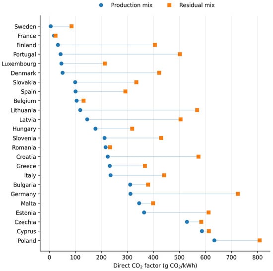
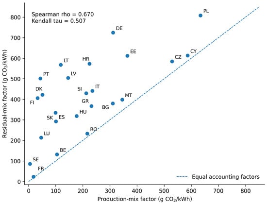
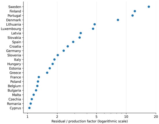
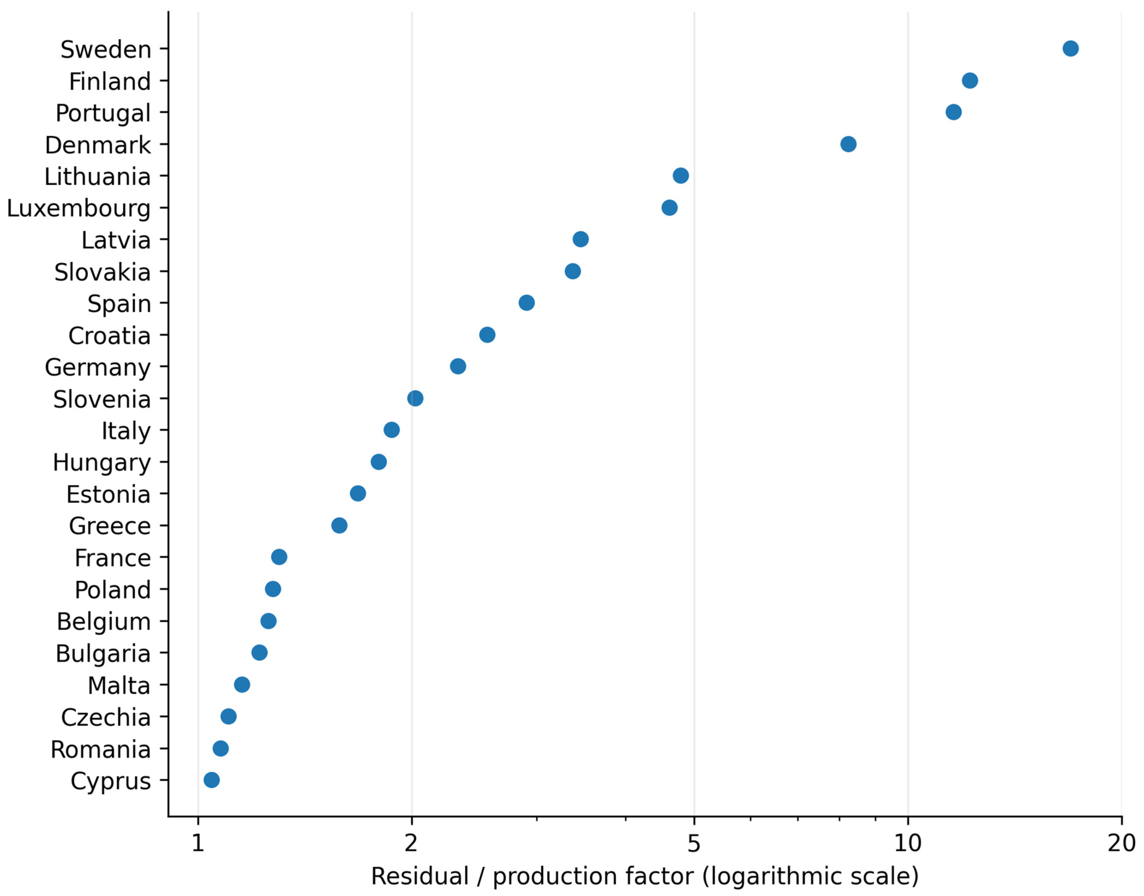
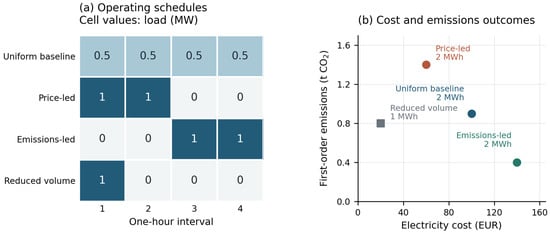
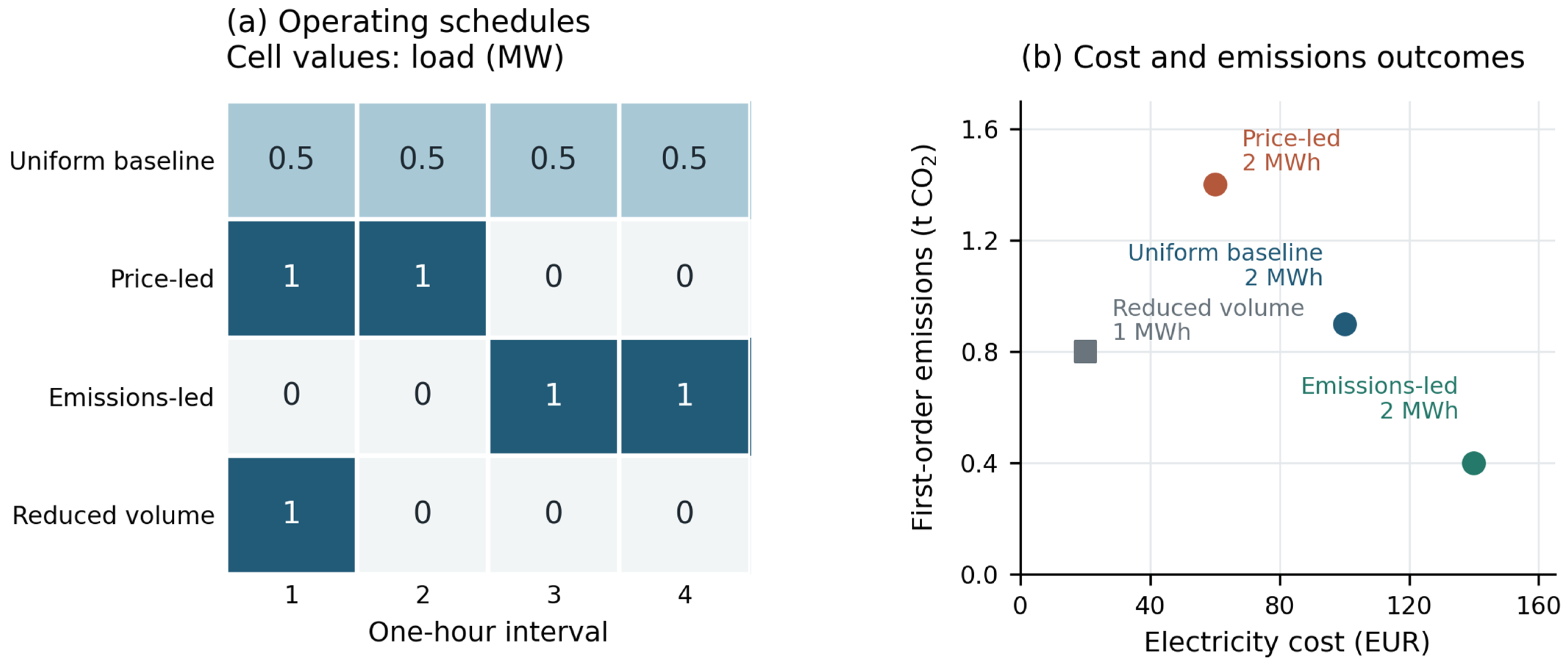

Disclaimer/Publisher’s Note: The statements, opinions and data contained in all publications are solely those of the individual author(s) and contributor(s) and not of MDPI and/or the editor(s). MDPI and/or the editor(s) disclaim responsibility for any injury to people or property resulting from any ideas, methods, instructions or products referred to in the content. |
© 2026 by the authors. Licensee MDPI, Basel, Switzerland. This article is an open access article distributed under the terms and conditions of the Creative Commons Attribution (CC BY) license.