


Abstract
High renewable penetration creates spatiotemporal mismatches between intermittent generation and rigid demand, making market-oriented electricity pricing critical for activating demand-side flexibility. Hypothesizing that state-contingent price adjustment, rather than temporal granularity alone, determines regulation efficiency, this study develops a unified price–load–dispatch coupling framework in which price, demand response and dispatch are solved jointly as a damped fixed point and compares four pricing mechanisms: regulated time-of-use (TOU) pricing, TOU–spot market coordination, real-time pricing (RTP), and a novel renewable-linked adaptive five-segment pricing (RL-AFSP) scheme. Using Shandong Province, China, a representative high-renewable-penetration region, as the case study, a customized improved particle swarm optimization (IPSO) algorithm quantifies each mechanism over 30 randomly drawn typical-day scenarios under a daily-energy-conserving demand-response model, with the tariff float ratios and time blocks taken from the official provincial schedule. Utilization is not monotone in price granularity: it rises from 86.33% under fixed TOU to 87.06% under TOU–spot coordination, falls back to 86.88% under RTP, and reaches its maximum of 88.19% under RL-AFSP, whose operating cost of 186.56 million CNY/day is also the lowest of the four (against 194.00 under fixed TOU). Real-time pricing therefore buys no technical advantage: RTP combines the widest intraday price swings (price coefficient of variation 81.7%), the highest revenue volatility (9.64%), the lowest daily profit (295.79 million CNY) and a price–load feedback that fails to converge within the 200-iteration cap. RL-AFSP converges in seven iterations and pairs the best technical performance with revenue volatility of 2.57% and the highest daily profit (575.68 million CNY). Against the static TOU benchmark its utilization and cost improvements are statistically significant (Holm-adjusted p = 1.86 × 10⁻⁸ and 1.68 × 10⁻⁸), and its advantage over RTP is robust to the price-sensitivity parameters, the adjustment band and demand elasticities from −0.15 to −0.40; at the weakest elasticity tested (−0.10) RTP attains a marginally lower cost, the single exception in the sweep, and is reported as such. Component ablation attributes the gain to state-contingent adjustment rather than to the bound itself, which instead guarantees convergence and limits revenue volatility. These simulation findings suggest that RL-AFSP is a candidate mechanism reconciling efficiency, economy and stability, offering policy-relevant insights for electricity pricing reform and source–grid–load–storage coordination, while requiring pilot validation before large-scale implementation.
1. Introduction
The global energy system is undergoing a profound transformation centred on decarbonization and digitalization. Driven by the dual pressures of climate change mitigation and energy security, accelerating the energy transition has become a global consensus and a core strategic priority [1]. In this context, the United Nations 2030 Agenda for Sustainable Development sets clear objectives, including a substantial increase in the share of renewable energy in the global energy mix [2]. As the central arena of the energy transition, the successful decarbonization of power systems hinges on the efficient and cost-effective integration of large-scale renewable energy sources such as wind and photovoltaic power, which are characterized by variability, intermittency and uncertainty (VIU).
However, the traditional power system operation and market mechanism were designed around dispatchable fossil-fuel-based generation, and their relatively static pricing schemes and dispatch logics are increasingly ill-suited to the challenges posed by high renewable energy penetration [3]. The core challenge lies in a pronounced spatiotemporal mismatch between electricity supply and demand, which implies that renewable generation is governed by natural conditions and exhibits limited controllability and anti-peaking characteristics (such as the mismatch between the “midday peak” of photovoltaic and the “evening peak” of load), while electricity consumption behaviour remains rigid, time-dependent, and highly concentrated. If this fundamental mismatch is not addressed through institutional and market-based innovations, it will lead to severe renewable curtailment, higher system balancing costs, and ultimately hinder the energy transition. Therefore, advancing electricity market and pricing reforms that accurately reflect the spatiotemporal value of electricity and real-time system conditions has become a central task in building a new-generation power system.
China’s energy transition strategy and electricity market development are currently at a critical stage. National policy directions explicitly call for deepening energy price reforms through market-oriented approaches and accelerating the construction of a unified national electricity market, with the aim of using market-based flexibility to facilitate the grid integration and utilization of renewable energy [4]. The latest policy guidelines on the signing and performance of medium- and long-term electricity contracts (e.g., Document No. 1502 issued by the National Development and Reform Commission) clarify the transition of market participants away from government-regulated time-of-use (TOU) tariffs toward pricing mechanisms formed through market negotiations that more dynamically reflect system marginal costs. This policy shift establishes both a clear institutional framework and a strong practical impetus for innovative research on electricity pricing mechanisms. In line with this objective, a series of policy documents have been issued to improve electricity price formation mechanisms and facilitate the participation of renewable energy in market-based transactions [5]. At the regional level, Shandong Province, one of China’s leading provinces in terms of renewable energy installed capacity, offers a benchmark case. The province has not only taken the lead in implementing a more refined five-segment TOU pricing scheme but has also issued implementation plans aimed at promoting the full participation of renewable energy in electricity market reforms [6]. These practices indicate that demand-side management centred on price signals is widely regarded as a critical lever for addressing system flexibility constraints and unlocking load-side adjustment potential [7].
Against this background, demand response and its core price-based instrument, the TOU pricing, have become increasingly important. By setting differentiated electricity prices across time periods, the TOU mechanism aims to convey signals of time-varying electricity costs to consumers, guiding them to optimize consumption patterns by shifting peak demand and increasing off-peak usage. In doing so, the TOU pricing seeks to achieve multiple objectives, including peak shaving and valley filling, improving overall system efficiency, and promoting renewable energy utilization [8,9,10]. Theoretically, the finer the “granularity” of the price signal (that is, the updated time scale and the accuracy reflecting the supply and demand state), the higher the efficiency of guiding resource allocation should be. However, there is an irreconcilable contradiction between the “static” nature and the “dynamic” nature of renewable energy output in the commonly implemented TOU mechanism which mostly uses pre-fixed time periods and spreads based on historical data or empirical judgement. When wind and photovoltaic output fluctuates sharply due to weather changes, the fixed peak and off-peak periods may not provide the correct incentive signals and may even generate perverse incentives, thereby constraining the full realization of TOU’s regulatory potential. Recent quasi-experimental evidence using a difference-in-differences design [11] also confirms that TOU pricing reduces electricity costs for industrial users, though the magnitude depends on the time-of-use structure.
Several studies have addressed the electricity price mechanisms and system optimization. Regions such as the European Union and the United Kingdom have adopted mechanisms including power purchase agreements (PPAs) and contracts for difference (CfDs) to enhance revenue stability for renewable energy investors, offering valuable institutional insights [12,13,14,15]. In contrast, research and practice in China have focused more on the localized application and optimization of TOU pricing. Provinces such as Jiangsu, Guangdong, and Sichuan have explored measures including seasonal critical peak pricing and more granular multi-period time segmentation tailored to regional load characteristics, promoting the evolution of the electricity price mechanism from the simple two-stage peak–valley structures to more refined multi-period designs [16,17,18,19]. Within this broader trend, Shandong Province’s five-segment TOU pricing scheme and the introduction of a “deep valley” price represent a typical and innovative example. These measures have achieved preliminary success in alleviating renewable energy curtailment during specific time periods [6]. However, these improvements are still not essentially detached from the framework of “fixed time periods, fixed spreads” or pre-adjustments based on seasonality, and their inherent limitations of “insufficiency signal accuracy and lack of dynamic adaptability” still exist when facing minute and hourly fluctuations in renewable energy [20]. Related experiences from mature retail markets, including the sales-side TOU policy review in [21] and Japan’s retail electricity management guidelines [22], also confirm that pricing granularity must be matched to users’ responsiveness.
Meanwhile, research on optimal dispatch in power systems with high renewable energy penetration has become increasingly sophisticated. There is a broad consensus in the literature that single-objective optimization, such as minimizing economic cost or carbon emissions alone, is no longer sufficient to meet the multi-dimensional coordination requirements of new-generation power systems involving multiple stakeholders [23,24]. Consequently, multi-objective optimal dispatch models that simultaneously account for economic efficiency, environmental performance, and high levels of renewable energy utilization have emerged as a major research focus [25,26,27]. However, model formulation represents only the first step. Solving such large-scale, nonlinear, high-dimensional optimization problems with multiple constraints poses a substantial computational challenge in its own right. Traditional mathematical programming approaches, including linear programming [28] and quadratic programming [29], often encounter severe computational bottlenecks as system scale expands. Metaheuristic algorithms are therefore widely adopted, among them particle swarm optimization (PSO) [30], the artificial bee colony algorithm [31], biogeography-based optimization [32] and the multi-verse optimizer [33]; yet these algorithms commonly suffer from slow convergence, susceptibility to local optima and insufficient solution accuracy when dealing with complex constraints [34,35,36,37,38,39,40,41,42]. Numerous improvement strategies have been proposed—enhancing population diversity through clustering [43], pseudo-gradient search [44], integrating chaotic mechanisms to improve ergodicity [45], adding forgetting factors within adaptive frameworks such as CAPSO [46], biogeography-based learning [47], hybrid differential-evolution PSO [48], IPSO coupled with wavelet neural networks for short-term load prediction [49], collaborative optimization of integrated power systems with CPSO [50], and PCANet/CNN + Bi-LSTM feature extraction for time-varying load characteristics [51]—but these approaches often fail to integrate effectively with the specific physical and operational constraints of power system dispatch. As a result, considerable room for improvement remains when such algorithms are applied to realistic and highly complex dispatch scenarios. The scalarisation precedent is drawn from multi-objective structural optimization [52]; within the energy domain, price-controlled smart-home energy management [53] and wind–CHP–heat-storage scheduling [54] couple operational dispatch with price signals.
Taken together, existing research and practice face a dual dilemma. At the mechanism level, the temporal granularity of current electricity price signals is insufficient to dynamically match the rapid fluctuations of renewable energy generation, creating a gap between the demand for high-efficiency renewable energy utilization and rigid pricing signals. This gap is particularly prominent under the existing government fixed pricing model and urgently needs to be filled through market-oriented mechanism innovation. At the technical level, there remains a lack of effective and robust tools capable of solving the complex price–load–dispatch coupled models, which constrains the ability to conduct fine-grained, quantitative evaluation and optimization of alternative electricity pricing mechanisms. Accordingly, the central research question of this study is: how can an electricity pricing mechanism be designed to simultaneously achieve high dynamic responsiveness and strong practical implementability and how can its overall performance in power systems with high renewable energy penetration be systematically evaluated through reliable quantitative methods?
To address those questions, this study advances the core hypothesis that signal precision determines regulation efficiency and develops a unified price–load–dispatch coupling analytical framework. The main contributions of this study are threefold. First, in terms of theoretical framework innovation, this study explicitly identifies the temporal granularity of electricity prices as a key variable linking market signals to system operational efficiency. On this basis, a systematic analytical framework is established to elucidate the transmission mechanisms and performance impacts of electricity price signals with different levels of granularity, ranging from static TOU pricing to real-time pricing on renewable energy utilization, system operating cost, and market stability. Second, in terms of pricing mechanism design, this study proposes a novel renewable-linked adaptive five-segment pricing (RL-AFSP) mechanism. Building upon the structural stability and user familiarity of the existing five-segment TOU pricing scheme, the proposed mechanism introduces two dynamic state variables, which are the renewable surplus index and the load pressure index, allowing electricity prices in each time segment to adaptively adjust in response to ultra-short-term system supply–demand conditions. In doing so, RL-AFSP seeks an optimal balance between dynamic precision in price response and policy implementability. Third, in terms of methodological innovation, to address the challenges posed by the high dimensionality, nonlinearity, and multiple constraints of the price–dispatch coupled optimization problem, this study designs a deeply customized improved particle swarm optimization (IPSO) algorithm. By embedding a constraint feasibility preservation mechanism, hybrid local search strategies, and adaptive parameter adjustment schemes, the proposed IPSO algorithm improves convergence speed, solution accuracy, and stability in complex power system dispatch problems, thereby providing robust technical support for mechanism evaluation.
This paper uses Shandong Province, one of China’s frontier regions in renewable energy development, as an empirical case and applies the proposed IPSO algorithm to quantitatively compare and analyze the combined performance of four mechanisms by using fixed TOU pricing, TOU–spot market coordination, real-time pricing, and the proposed RL-AFSP mechanism. The empirical results not only validate a series of hypotheses regarding the relationship between electricity price temporal granularity and system performance but also reveal an “advantage aggregation” effect of RL-AFSP in jointly achieving high renewable energy utilization, low system operating cost, and high revenue stability. These findings offer an innovative and operationally feasible solution for electricity pricing reform and system operation in regions with high renewable energy penetration.
The remainder of this paper is organized as follows. Section 2 reviews the implementation background, performance, and limitations of the existing five-segment TOU pricing scheme in Shandong Province. Section 3 presents the price–load–dispatch coupling modelling framework based on the IPSO algorithm and details the design of the RL-AFSP mechanism. Section 4 introduces the scenario design and data sources. Section 5 reports and discusses the empirical results. Section 6 summarizes the main conclusions and proposes targeted policy implications. Section 7 outlines the limitations of this study and directions for future research.
2. The “Five-Segment” Electricity Price Mechanism in Shandong Province: Implementation Status, Effectiveness, and Limitations
As a forerunner in China’s energy transition, Shandong Province faces system operation challenges that are highly representative of those arising from large-scale renewable energy integration. As of May 2025, the province’s total installed renewable energy capacity had reached 125 GW, with its photovoltaic capacity ranking first nationwide [55,56]. Behind this achievement lies the emergence of two structural contradictions. First, there is a serious mismatch in the source-load sequence, where the “midday peak” of photovoltaic power generation is difficult to connect with the “evening peak” of residential electricity consumption, resulting in an “inversion of supply and demand”. Second, the supply of system flexibility remains insufficient to smooth the inherent stochasticity, volatility, and intermittency of wind and solar generation, thereby exacerbating the risk of renewable curtailment [57]. Under these conditions, the traditional two-period peak–valley pricing scheme, characterized by overly coarse signals, is no longer capable of providing effective incentives for precise load shifting.
To address these challenges, Shandong Province has taken the lead nationwide in exploring and implementing a five-segment TOU pricing mechanism. The core innovation of this mechanism lies in dividing the daily electricity consumption profile into five refined segments: sharp peak, peak, shoulder, off-peak, and deep valley periods. Its design logic aims to mitigate spatiotemporal mismatches through multi-dimensional coordination. On the generation side, it provides clear price signals and economic incentives for flexibility resources such as energy storage to participate in peak regulation. On the grid side, it seeks to guide loads to shift from high-price to low-price periods, thereby reducing peak–valley differentials and alleviating network congestion and curtailment pressures. On the demand side, it directly incentivizes industrial, commercial, and residential users to proactively adjust consumption behaviour in response to price signals [55,56]. This policy practice has evolved over several decades. It began with an initial pilot in Jinan in 1994, marking a pioneering effort nationwide [58], expanded to cover industrial and commercial users in 2021 [59], and was further extended in 2023 to residential and agricultural sectors with the introduction of a dynamic “critical peak–deep valley” adjustment mechanism [60], forming a relatively complete policy system. The “Complementation Plan for market-oriented Reform of Feed-in Tariffs for New Energy in Shandong Province (Draft for Comment)” released in 2025 aims to promote the full participation of new energy in the electricity market and form synergy with the existing TOU pricing scheme, marking the deepening stage of the reform [6].
In terms of implementation outcomes, the five-segment TOU pricing mechanism has delivered positive results across multiple dimensions. From an economic perspective, it has effectively reduced users’ overall electricity costs by incentivizing peak shaving and valley filling. Environmental benefits have also been significant, as the system’s ability to absorb photovoltaic generation during midday high-output periods has been substantially enhanced, and portions of peak demand have been successfully shifted, facilitating full or high-level utilization of renewable electricity [56]. The social benefits are reflected in the improvement of the overall operational efficiency and supply reliability of the power grid through the optimization of power resource allocation. These outcomes suggest that, compared with simple two-period pricing schemes, more refined time segmentation can better reflect the actual marginal cost of electricity and the degree of system tightness at different times, thereby unlocking demand-side response potential.
Nevertheless, as renewable energy penetration continues to rise rapidly, the limitations of the five-segment TOU pricing mechanism have become increasingly evident. At their core lies a fundamental tension between the static nature of the mechanism and the highly dynamic characteristics of renewable generation. First, although the time periods are more finely divided, the basic pattern of “two peaks and two valleys” is still pre-fixed and relies on statistical predictions of historical load curves and new energy output patterns [61]. When the actual output of wind and photovoltaic power fluctuates sharply due to weather changes and deviates from the typical pattern, the fixed high-price (sharp peak and peak) or low-price (off-peak and deep valley) periods may not accurately match the real-time supply and demand status of the system, resulting in the “failure” or “mismatch” of the price signal, which cannot stimulate load transfer or consumption at the most needed moment. Second, although Shandong Province has established seasonal adjustments of time periods and prices, such ex ante seasonal or monthly adjustments still lack sufficient responsiveness, making it difficult to adapt to intraday or hourly renewable fluctuations, while the precision of adjustments remains limited. Consequently, under conditions of high penetration and strong volatility of renewable energy, the current mechanism faces the core challenges of insufficient signal precision and inadequate dynamic adaptability. Accordingly, this paper addresses these constraints and their implications for the full regulatory potential of the pricing mechanism.
3. Coupled Modelling Frameworks of “Electricity Price–Dispatch” Based on the IPSO Algorithm
3.1. Construction of Multi-Source Collaborative Optimization Scheduling Model
To systematically evaluate the overall impacts of different electricity pricing mechanisms in power systems with high renewable energy penetration, it is necessary to establish a mathematical model that captures the closed-loop coupling among price signals, load responses, and dispatch decisions. Given that a single optimization objective is insufficient to characterize the multi-dimensional requirements of such systems under high renewable penetration [62], this study develops a multi-objective optimal dispatch model. The core objectives of the model directly address two fundamental requirements of high-renewable power systems, which is under the rigid constraints of secure and economic system operation, to maximize the utilization of variable renewable energy while minimizing overall system cost. The proposed methodological framework draws on and extends the modelling approaches of Tan et al. (2019) [63] and Li and Qiu (2016) [64].
3.1.1. Objective Function
The objective function mainly includes minimizing the total economic input of the system MinZ and maximizing its absorption capacity MaxW. The total economic input of the system mainly includes fixed costs CFIX, operating costs CRUN, maintenance costs CMAIN, and fuel costs CFU. To characterize the social resource waste and environmental costs resulting from the failure to absorb a high proportion of renewable energy, wind curtailment costs CCURT are introduced, and the calculation formulas are as follows:
where CFIX,RUN represents fixed costs and operating costs, Ch,Cf,Cc,Cg, indicating the fixed costs and operating costs of thermal power, wind power, storage, solar power and nuclear power, Nh,Nf,Nc,Ng,Nk, respectively representing the number of units put into operation of thermal power, wind power, storage, solar power and nuclear power.
where CMAIN represents maintenance costs, Cm,h,Cm,f,Cm,c,Cm,g, indicating the unit maintenance costs of thermal, wind, storage, solar and nuclear power, P,Pf,t,Pc,t,Pg,t,Pk,t, respectively representing the output of thermal, wind, storage, solar and nuclear power during the time period;
where CFU,co represents the fuel cost of coal-fired power, aj,bj,cj is the coefficient of the fuel consumption function of the unit, Pj,t is the output of the unit during the period, and Pco is the unit price of coal;
where CFU,nu is the coefficient of the fuel consumption function of the unit, aj, bj, cj, Pj,t is the output of the unit j during t the period, and Pnu is the unit price of nuclear power;
where CCURT represents the cost of wind power curtailment, PFORECAST,t is the predicted power generation of renewable energy during the period, PW,t is the actual power generation of renewable energy during the period, and ω is the penalty factor;
where MaxW represents the core goal pursued to address the challenge of integrating a high proportion of renewable energy into the grid renewable energy absorption capacity, Wf,t represents the consumption of wind power in a certain period, Wg,t represents the consumption of photovoltaic power in a certain period, and T represents the total number of periods.
MinZ = CFIX + CRUN + CMAIN + CFU + CCURT
Because the two objectives of Equations (1) and (2) conflict, they are not solved as a strict Pareto problem. They are combined by weighted-sum scalarisation: maximizing the absorbed renewable energy W is equivalent to minimizing the curtailed energy, which is already priced inside Z through the curtailment term of Equation (7). The optimization therefore solves a single scalar objective.
where the curtailment energy is defined on the dispatched-versus-available convention, so that its sign is unambiguous:
where the superscript “avail” denotes the available (forecast) output and the unadorned symbol that the output actually dispatched, so that Pcurt,t is non-negative by construction. The renewable energy utilization rate is correspondingly defined on energy quantities over the whole day rather than by summing instantaneous power values:
with Δt = 1 h. No Pareto front, hypervolume or inverted-generational-distance analysis is provided because the weight ωcurt is fixed a priori; the cost–absorption trade-off is instead explored through the sensitivity sweeps of Section 5.2. This scalarised formulation is referred to below as the weighted-sum dispatch model.
3.1.2. Technical Constraints of Thermal Power Units
Capacity constraints of thermal power units:
Ph,min ≤ Ph,t ≤ Ph,max ∀t
Minimum start and stop time constraints:
Ton,h ≥ Tmin,on,h and Toff,h ≥ Tmin,off,h
Climbing rate constraint:
where Ph,min,Ph,max represents the minimum and maximum output of the thermal power unit i; Ton,h,Toff,h indicates the continuous operation and downtime of unit i. R±,h,R∓,h respectively represent the up and down climbing rate constraints of unit i.
Ph,t − Ph,t−1 ≤ R±,h and Ph,t−1 − Ph,t ≤ R∓,h
The following technical constraints jointly constitute the physical boundaries that ensure the safe and stable operation of power systems with high renewable energy penetration. In particular, ramping constraints and system coupling constraints are critical for mitigating renewable energy variability and achieving real-time power balance.
3.1.3. Technical Constraints of Nuclear Power Units
Capacity constraints of nuclear power units:
Pk,min ≤ Pk,t ≤ Pk,max ∀t
Climbing rate constraint:
where Pk,min,Pk,max represents the minimum and maximum output of the nuclear power unit i; Ton,k,Toff,k indicates the continuous operation and downtime of unit i; R±,k,R∓,k respectively represent the up and down climbing rate constraints of unit i.
Pk,t − Pk,t−1 ≤ R±,k and Pk,t−1 − Pk,t ≤ R∓,k
3.1.4. Technical Constraints on Wind Power and Photovoltaic Power
Real-time output constraint of wind power:
Pf,t ≤ Pf,max × ηf,t ∀t
Constraints on wind energy utilization of wind turbine units:
ηf,t ≤ ηf,max
Real-time output constraint of photovoltaic:
Pg,t ≤ Pg,max × ηg,t ∀t
Constraints on the utilization of light energy by photovoltaic units:
where Pf,t is the output of the wind farm during the period, Pf,max is the maximum output of the wind farm, ηf,t is the wind energy utilization coefficient during the period, Pg,t is the output of the photovoltaic power during the period, Pg,max is the maximum output of the photovoltaic power, and ηg,t is the wind energy utilization coefficient during the period.
ηG,t ≤ ηG,max
3.1.5. Technical Constraints of Energy Storage Power Stations
In power systems with high renewable energy penetration, energy storage serves as a critical source of flexibility, and its charging and discharging constraints directly determine the system’s capability to regulate variable renewable generation.
Maximum and minimum charge and discharge capacity constraints of energy storage systems:
Emin ≤ Et ≤ Emax ∀t
Maximum and minimum charging rate constraints:
Minimum and maximum discharge rate constraints:
where Emin,Emax respectively represent the minimum and maximum values allowed for energy storage capacity; , respectively represent the maximum and minimum charging rates of the energy storage system; , respectively represent the maximum and minimum discharge rates of the energy storage system.
The above limits are complemented by the intertemporal energy balance. Let Et denote the stored energy at the end of period t, with charging and discharging efficiencies η_ch and η_dis, respectively, explicitly accounted for:
The state of charge is bounded and the initial and terminal conditions are imposed so that the storage neither starts nor ends the day with an arbitrary energy level:
Simultaneous charging and discharging is excluded by binary indicators, and the rated power limits are distinguished from the energy capacity limits of Equations (21)–(23):
In the case study Einit = 5000 MWh and Emax = 15,000 MWh are energy quantities expressed in MWh, whereas the charging and discharging power limits are expressed in MW; the storage parameter table in Section 4.2 reports the two explicitly and separately. A cycling cost of 100 CNY/MWh is charged on each charge and discharge event, which represents degradation in reduced form.
3.1.6. System Coupling Constraints
The power balance constraint constitutes the core of system operation in power systems with high renewable energy penetration. It must continuously coordinate the outputs of variable renewable generation, dispatchable generation, load demand, and energy storage actions, serving as the point at which electricity price signals ultimately translate into physical system operation.
Power balance constraints:
where Ph,t, Pf,t, Pk,t and Pg,t denote the dispatched output of thermal, wind, nuclear and solar generation in period t; Pch,t and Pdis,t are the charging and discharging power of the energy storage station, modelled as two separate non-negative variables so that charging and discharging are never netted against each other; Dt is the price-responsive demand of Equation (28); and Pcurt,t is the curtailed renewable power defined by Equation (10). The model is an aggregated single-bus generation-demand balance: transmission line capacity, network losses, voltage limits and regional congestion are not represented, so curtailment here arises only from the aggregate supply–demand balance, and the conclusions should not be read as establishing provincial-level network feasibility.
Ph,t + Pf,t + Pk,t + Pg,t + Pdis,t = D_t + Pch,t + Pcurt,t ∀t
3.1.7. Price-Responsive Demand Model
The coupling claimed in the title requires that price changes actually move demand and that the demand used to form the price signal is itself the demand produced by that price. Both links are formalized below. Let D0t and p0t denote the baseline demand and the reference five-segment tariff, respectively. Users respond through a multiplicative constant-elasticity shift:
where ε < 0 is the self-price elasticity. Because the interest here is load shifting rather than load growth, the response is renormalized so that daily energy is exactly conserved:
Participation is bounded so that no period is shifted beyond a technically and contractually plausible range, and the aggregate shift is capped. The single-period band is itself the source of the aggregate cap: because |Dteff − Dt0| ≤ 0.30 Dt0 holds in every period, summation over t gives Σt |Dteff − Dt0| ≤ 0.30 Σt Dt0, so κ = 0.30 follows directly from the 0.70–1.30 band rather than being an independently chosen parameter. The aggregate constraint is therefore redundant with, and never tighter than, the single-period constraint; it is retained only to state the participation limit explicitly. The aggregate cap is inactive in every reported case: the realized aggregate shift is 0.00% of daily energy under the fixed five-segment benchmark, 2.67% under RL-AFSP and 2.68% under its unbounded variant, against the 30% cap (Load shift column of the mechanism-ablation table in Section 5.2). For the bounded mechanism RL-AFSP the single-period band is likewise inactive: its adjustment coefficient is confined to mt ∈ [0.6, 1.6], which at ε = −0.15 confines the per-period response to [0.93, 1.08] times the baseline before renormalisation and to [0.86, 1.16] after it, in both cases strictly inside the 0.70–1.30 band. The participation constraints thus delimit the feasible set without binding at any reported optimum.
This feedback is then obtained as a fixed point rather than by a single forward pass. Prices are formed from the current demand estimate, demand responds to those prices, and the two steps are iterated with under-relaxation until the demand profile stops moving:
where f is the pricing rule of the mechanism under study, DR denotes Equation (28) with the renormalisation of Equation (29), λ = 0.5 is the damping coefficient, τ = 10−4 the tolerance and the iteration cap is 200. The adjustment coefficient mt defined in Section 4.1 is evaluated on the responded demand Dteff rather than on the baseline demand, which closes the loop. Convergence is itself an informative result: fixed TOU converges in one iteration by construction, and the TOU–spot hybrid and RL-AFSP converge in about seven iterations to an equilibrium that is insensitive to λ, whereas real-time pricing reaches no fixed point within the cap and its outcomes depend on the termination rule, as quantified in Tables S5 and S6 of the Supplementary Material.
3.2. Customized IPSO Algorithm
Solving the price–load–dispatch coupled model of Section 3.1 requires handling a 96-dimensional, nonlinear and multi-constrained search space, for which this study develops a customized improved particle swarm optimization (IPSO) algorithm.
Standard PSO is widely used for such problems because of its simple structure and fast convergence [30,44,65], but three weaknesses limit its direct application here: particles frequently leave the feasible region because constraints are handled only as penalties; population diversity decays in later iterations, causing premature convergence; and fixed inertia and learning factors cannot adapt to the differing exploration and exploitation needs of the search stages.
3.2.1. Three Components of the Customized IPSO
IPSO therefore adds three components to standard PSO: a constraint feasibility maintenance mechanism, a hybrid local search strategy, and an adaptive parameter schedule.
(1) Constraint feasibility maintenance mechanism: precise embedding and proactive repair of physical constraints.
Because the model couples many physical constraints, a repair operator is embedded after every particle update so that infeasible particles are projected back onto the feasible manifold rather than merely penalized.
Power balance constraint repair: If there is a power gap after the particle update (), the regulation amount is allocated based on the principle of “minimizing marginal regulation cost”—prioritizing the correction of the charging and discharging power of the energy storage (ΔPstorage = ΔP). If the energy storage reaches the charging and discharging power boundary, then allocate the remaining regulation capacity in the order of the flexibility of unit regulation (thermal power > nuclear power > adjustable new energy) to ensure that strictly holds.
Boundary constraint repair for energy storage SOC (State of Charge): Let the safety range of the energy storage SOC be [SOCmin,SOCmax]; if SOCt < SOCmin after the update, it will be forcibly adjusted to SOCt = SOCmim, and at the same time, the weight of the next round of charging speed of this particle will be reduced. If SOCt > SOCmax, adjust it to SOCt = SOCmax, and increase the discharge speed weight to avoid overcharging and over-discharging of the energy storage.
(2) Hybrid local search strategy: fine-grained optimization in the later stage of iteration.
To counter the loss of diversity and premature convergence in later iterations, a hybrid local search is applied around the incumbent global best.
Gradient-approximation local search: a finite-difference direction is estimated in the neighbourhood of the global best and a bounded step is taken along it, refining the solution without disturbing the swarm.
(3) Parameter-adaptive adjustment strategy: dynamic optimization oriented to the scheduling process.
The setting of key algorithm parameters (inertia weight w, cognitive learning factor c1 and social learning factor c2) has a decisive impact on search performance. This algorithm abandons the fixed parameter mode and adopts an adaptive strategy that is linked with the optimization process and the state of constraint satisfaction:
Inertia weight w: a constraint-adaptive non-linearly decreasing schedule starting from 0.9, which emphasizes exploration early and exploitation later.
Learning factors: c1 decreases linearly from 2.0 to 1.0 and c2 increases from 1.0 to 2.0, shifting the balance from individual cognition to social information as the search proceeds.
The basic update equation of the algorithm is shown in Equation (32), and its solution process ensures the efficient and stable acquisition of high-quality scheduling schemes under complex constraints.
The basic equation of the particle swarm optimization algorithm is as follows:
where vij(t) is the velocity of the particle i in the dimension j, xij(t) is the position of the particle i in the dimension j, w is the inertia weight, c1 and c2 are the learning factors, r1j(t) and r2j(t) are random numbers within the interval [0, 1], pij, is the historical optimal position of the particle, and gj is the global optimal position.
3.2.2. Benchmark of IPSO Against Standard PSO
IPSO is validated at two levels, both reported in full in the Supplementary Material. First, on the dispatch problem itself we compare five search operators under an identical protocol: the same 96-dimensional instance, population size 40, iteration budget 80, random initialization, the same constraint-repair module, the same stopping rule and the same 30 seeds (1000–1029). Only the search operator differs, so the comparison is fair.
Table 1 summarizes the results. The mean post-repair operating cost is 1.9307 × 10⁸ CNY/day for the full IPSO, against 2.0179 × 10⁸ without feasible initialization, 2.1101 × 10⁸ for chaotic PSO, 2.1270 × 10⁸ for standard PSO and 2.1568 × 10⁸ for DE/rand/1/bin; the IPSO also has the smallest run-to-run standard deviation (3.12 × 10⁶ versus 12.52 × 10⁶ for standard PSO) and the highest number of runs meeting the balance tolerance (14/30 versus 0/30). A reference row with the repair module ablated (2.6030 × 10⁸) shows that constraint handling, not the search operator, is the largest single contributor to solution quality on this problem, which is why the fair protocol matters. Convergence speed is comparable rather than superior (59.0 iterations to within 1% of final, against 51.7 for standard PSO); the corresponding mean convergence curves of all six configurations are plotted in the convergence figure presented in Section 4.2. Wall-clock cost per run is of the same order for all five operators on the same hardware (0.36–0.48 s/run, reported as the median of five repeated 30-draw passes so that transient machine load cannot distort the ranking), with the full IPSO at 0.36 s against 0.40 s for standard PSO and 0.48 s for DE; we therefore claim no runtime premium and, likewise, no convergence-speed advantage. Second, on standard test functions (the IEEE CEC2017 and CEC2022 benchmark suites; dimensions 10 and 30, 30 independent runs each, identical evaluation budget) the IPSO significantly outperforms standard PSO (15/15 functions), GA (15/15) and GWO (13–14/15), with the Friedman test rejecting identical distributions (p < 1 × 10⁻⁸). It does not outperform DE, which attains the best average rank (1.20–1.27 versus 1.87–2.07 for the IPSO) and wins on 11–13 of 15 functions. Third, a component ablation over the 30 function instances shows that all three IPSO components contribute: the full configuration reaches an average rank of 1.73 and is best on 20/30 instances (1.04× the best mean), whereas standard PSO ranks 5.00 and is never best (931×). Taken together, the evidence supports positioning IPSO as a problem-tailored improvement for constrained dispatch, whose adaptive parameters, stagnation mutation and local search are each justified, rather than as a universally dominant optimizer. On the dispatch problem specifically, it is the best of the five operators compared; on unconstrained benchmark functions DE remains stronger.
Table 1.
Comparison of algorithms on the dispatch problem (identical problem instance, population size 40, iteration budget 80, random initialization, shared constraint-repair module and random seeds 1000–1029; 30 independent autumn typical days. Only the search operator differs among the first five rows. The last row removes the repair module from standard PSO to isolate the contribution of constraint handling. Tolerance = maximum power balance violation below 0.5% of mean load.).
The solution procedure of the price–dispatch model developed in this paper is shown in Figure 1.
Figure 1.
The process of improving the particle swarm optimization algorithm.
4. Study Scenario Design and Data
4.1. Scenario Simulation and Theoretical Hypotheses
Building on the coupling framework of Section 3, four pricing mechanisms are compared under identical system data, and three hypotheses are tested.
H1 (Efficiency improvement hypothesis).
Electricity price time granularity is positively correlated with the efficiency of renewable energy consumption.
H2 (Cost optimization hypothesis).
The time granularity of electricity prices is negatively correlated with the overall operating cost of the system, and the construction is positively correlated with the improvement of consumption efficiency.
H3 (Benefit trade-off hypothesis).
The time granularity of electricity prices is negatively correlated with the stability of market benefits.
To test these hypotheses, we construct a renewable-linked adaptive five-segment pricing (RL-AFSP) mechanism that keeps the provincial five-segment tariff structure and adjusts it through two bounded state indices.
The specific design of RL-AFSP is as follows:
(1) System operational status quantification indicators: Define two complementary dimensionless indices to quantify the operational status of high-proportion renewable energy systems in real time.
Renewable surplus index (St): measures the extent to which high-proportion renewable energy generation exceeds the system’s absorbable net load. The formula is , where is the predicted generation of renewable energy at time t, and At = max (Dt − Pnuc − Pcoal,min, ε) is the net-load absorption headroom at time t, i.e., the load remaining after subtracting must-run nuclear output Pnuc and the minimum technical output of the coal fleet Pcoal,min (ε a small positive constant). Normalizing by At rather than by the gross load Dt is essential in systems with large must-run baseload: renewable output that exceeds the absorbable headroom cannot be absorbed even when it is below total load because coal and nuclear units cannot be turned down below their technical minimum. St > 0 indicates an oversupply of renewable energy relative to the absorbable headroom. The higher the value of St, the higher the surplus degree.
Load pressure index (Lt): measures the system’s reliance on conventional sources and peak load pressure. The formula is ; Lt > 0 indicates that renewable output is insufficient and the residual load must be supplemented by conventional sources; the larger the value, the more significant the load pressure. Both indices are normalized by the absorbable headroom At rather than by the gross load, so that they reflect the marginal condition faced by the dispatchable fleet.
(2) Price-adaptive adjustment coefficient: Based on the above index, a dynamic adjustment coefficient is constructed to achieve a precise mapping of the price to the system state.
where α > 0 is the sensitive parameter of price to renewable surplus. The more renewable surplus there is, the greater the reduction in electricity price will be. β > 0 is the price-sensitive parameter to load pressure; the tighter the system, the greater the increase in electricity price. To avoid excessive fluctuations in electricity prices, set the upper and lower limits of the adjustment coefficient: . It is recommended to take values of mmin = 0.6 and mmax = 1.6 to balance flexibility and stability.
mt = 1 − αSt + βLt
(3) Adaptive electricity price structure: attain a five-segment structure of “sharp peak, peak, shoulder, off-peak, and deep valley”, and only make dynamic fine-tuning of the electricity price value during the period.
where is the benchmark price for the period to which time belongs, and z(t) is the period identification function.
(4) Time-slot boundary fine-tuning: Under sustained renewable surplus or sustained load pressure, the segment boundaries may shift by at most one position, which keeps the schedule recognizable while letting it follow the system state.
(5) Integration: The adjusted prices feed the demand-response model and the resulting load feeds the dispatch model, closing the price–load–dispatch loop described in Section 3.1.7.
Four mechanisms are defined to span the granularity spectrum.
Mechanism 1 (fixed TOU) is the static five-segment schedule, the status quo benchmark.
Mechanism 2 (TOU–spot hybrid) blends the five-segment tariff with a bounded marginal-cost spot component at 40% weight, giving medium granularity.
Mechanism 3 (real-time pricing) pushes granularity to its extreme: the price follows the net-load position continuously over the full range [0.10, 2.50] times the shoulder-period base price, without the bounded adjustment that characterizes RL-AFSP.
Mechanism 4 (RL-AFSP) retains the five-segment structure and adjusts it continuously within [0.6, 1.6] through the two bounded state indices, combining high granularity with bounded adjustment.
(6) Demand-response model. Users respond through a multiplicative constant-elasticity shift, D’t = D0t (pt/pref,t)ε, renormalized so that daily energy is conserved; the response is therefore a pure intertemporal load shift. The self-elasticity baseline is ε = −0.15, within the empirical range for industrial and commercial users, and is varied from −0.10 to −0.40 in Section 5.2. Each period is additionally bounded to [0.70, 1.30] of its baseline as a safety rail.
The four mechanisms form a nested design so that granularity can be identified: they share the same five-segment base tariff, net-load signal, demand-response model, system data and solver, differing only in how often and how freely the price may move—never for fixed TOU, by segment with a bounded spot component for the hybrid, continuously and unbounded for RTP, continuously within [0.6, 1.6] for RL-AFSP. Section 5.2 adds a ladder that varies only the number of daily updates.
4.2. Data Sources and Typical-Day Simulation Design
The case study is calibrated to Shandong Province; Table 2 classifies every input as observed, constructed, calibrated or assumed, and Table S1 of the Supplementary Material gives the full provenance. The simulation covers one representative day at one-hour resolution, with autumn (September–November) as the main case and spring as a robustness check, using the five-time blocks and float ratios of the official provincial schedule for September–November [66,67]. Macro-level indicators—installed capacity, renewable share and planning information—are observed data from publicly available government documents, the national statistical yearbook and provincial planning notices [68,69,70,71,72], all cited with accessible links. The hourly demand, wind and solar series are constructed typical-day profiles, not raw extracts from an external database: the day is divided into the five segments, each is assigned a plausible interval from annual and seasonal data, and hourly values are drawn uniformly within them. Each of the 30 simulated days (seeds 1000–1029) is one such draw, and the results are averaged over them, so sampling variability is propagated into the reported uncertainty. Storage parameters follow the China Electricity Council’s Annual Industry Statistics of Electrochemical Energy Storage Power Stations for 2024, released on 27 March 2025 [73], whose full text is publicly reproduced at the URL given in that reference; the reported fleet-wide round-trip efficiency of 88.75% and grid-side comprehensive efficiency of 81.71% bracket the 0.85 and 0.90 values adopted here. Because the originally constructed renewable series implied almost no curtailment pressure—below 0.3% of renewable generation—the mechanisms were technically indistinguishable and H1–H3 untestable; a documented penetration multiplier kpen was therefore introduced and set to 2.4, the value whose status quo utilization reproduces the level associated with Shandong’s high-penetration conditions (scan in Table S3). The implied 63 GW wind and 67 GW solar is consistent with the reported provincial renewable capacity of roughly 125 GW, an independent check on the calibration.
Table 2.
Classification of variables and data sources in the simulation.
Reproducibility note. The objective is a weighted-sum scalarisation, not a strict Pareto formulation: total operating cost plus a renewable-curtailment penalty. Coal is 350 CNY/MWh and nuclear 320 CNY/MWh; wind and solar marginal generation costs are zero because capital cost is sunk in a dispatch problem, with their curtailment penalties of 250 and 220 CNY/MWh representing the opportunity cost of spilled energy; storage cycling costs 100 CNY/MWh per charge or discharge event; the balance soft constraint carries 1000 CNY per MW of violation. Renewable utilization is defined on energy quantities over the day—absorbed renewable energy divided by available renewable energy, Δt = 1 h. Revenue volatility is reported on two distinct bases that are never mixed: the coefficient of variation of daily revenue across the 30 days and that of hourly revenue within a day. Prices are formed from day-ahead forecasts and the same forecast series drives the dispatch, so forecast error enters only through the scenario intervals, the elasticity sweep and the Monte Carlo analysis (Table S22). The price functions, demand-response model, fixed-point iteration and full IPSO schedule are given in Part 2 of the Supplementary Material, and the accompanying scripts, which are supplied on request, reproduce every number in Table 1, Table 2, Table 3, Table 4 and Table 5 and Figure 2, Figure 3, Figure 4, Figure 5, Figure 6, Figure 7, Figure 8, Figure 9 and Figure 10 from the documented seeds.
Table 3.
Technical parameters of the energy storage system.
Table 4.
Computational results of the four pricing mechanisms.
Table 5.
Comparison of the four mechanisms. Bold type marks the header row and the mechanism labels in the first column.
Figure 2.
Spring-scaled electricity demand and predicted wind power output ranges over the five segments of the official September–November schedule adopted in this study.
Figure 3.
Autumn electricity demand and predicted wind power output ranges over the five segments of the official September–November schedule adopted in this study.
Figure 4.
Spring-scaled predicted photovoltaic output over the five segments of the official September–November schedule adopted in this study.
Figure 5.
Autumn predicted photovoltaic output over the five segments of the official September–November schedule adopted in this study.
Figure 6.
Comparison of renewable energy utilization rates among different mechanisms.
Figure 7.
Comparison of operating costs among different mechanisms.
Figure 8.
Comparison of electricity price revenue results by mechanism.
Figure 9.
Comparison of profit results by mechanism.
Figure 10.
Mean convergence curves of the six algorithm configurations benchmarked in Table 1 (identical problem instance, population size 40, iteration budget 80, shared constraint-repair module; averaged over 8 independent typical days and plotted separately from the 30-day statistics in Table 1 to keep the figure readable. The logarithmic vertical axis is the penalized objective. Removing the repair module (grey dashed) leaves the search far above all other configurations, and the full IPSO (red solid) attains the lowest plateau.).
5. Results and Analysis
The results for the calibrated Shandong case are summarized in Table 4 and Table 5 and Figure 2, Figure 3, Figure 4, Figure 5, Figure 6, Figure 7, Figure 8, Figure 9 and Figure 10.
Fixed TOU mechanism: verifying the limitations of “stability first”
Under the fixed TOU benchmark, the price is static, so no load is shifted: utilization is 86.33%, operating cost 194.00 million CNY/day, daily revenue 713.01 million and revenue volatility only 1.00%, the lowest of the four mechanisms.
TOU and spot market mechanism: marginal improvements as a transitional outcome
Adding a bounded spot component (TOU–spot) raises utilization to 87.06% and lowers cost to 189.35 million CNY/day, at the price of higher revenue volatility (3.49%) and a substantial fall in daily revenue to 623.56 million, because part of the load is shifted into cheaper periods.
Real-time pricing mechanism: unbounded price movement buys no technical advantage
Real-time pricing does not attain the best technical performance. Its utilization of 86.88% is below that of the coarser TOU–spot hybrid (87.06%) and 1.31 points below RL-AFSP, and its operating cost of 188.89 million CNY/day is above the 186.56 million attained by RL-AFSP; both disadvantages are significant (Holm-adjusted p = 9.13 × 10⁻⁸ and 9.94 × 10⁻⁵; Cliff’s delta +0.48 and −0.45 in favour of RL-AFSP). Its economic and stability properties are worse still: daily revenue falls to 484.68 million and profit to 295.79 million CNY/day, and revenue volatility rises to 9.64%, about 3.7 times that of RL-AFSP, with non-overlapping bootstrap intervals. More fundamentally its price–demand feedback does not converge: with prices permitted to span [0.10, 2.50] times the shoulder-level base price, the iteration reaches no stable equilibrium within 200 steps (0 of 30 days converge), and its outcomes vary widely across admissible damping coefficients (utilization by 8.02 percentage points, cost by 17.5% and revenue by 65.8%, Table S5). Its revenue and profit are therefore reported as an order-of-magnitude indication at one documented termination point, not as determinate values.
RL-AFSP mechanism: achieving an equilibrium solution for “advantage aggregation”
RL-AFSP reaches 88.19% utilization at 186.56 million CNY/day, with daily revenue of 762.24 million and profit of 575.68 million—the highest of the four—and revenue volatility of 2.57%, about one quarter of RTP. Against the static benchmark the improvements are large and statistically significant (+1.87 points and −7.44 million CNY/day, Holm-adjusted p = 1.86 × 10⁻⁸ and 1.68 × 10⁻⁸, Cliff’s delta +0.64 and −0.87, better in 100.0% and 100.0% of the 30 paired days). Against the hybrid both advantages are significant (+1.13 points, delta +0.42, adjusted p = 1.42 × 10⁻⁷; −2.79 million CNY/day, delta −0.48, adjusted p = 1.12 × 10⁻⁷). Against RTP it is superior on both counts (+1.31 points, delta +0.48, adjusted p = 9.13 × 10⁻⁸; −2.33 million CNY/day, delta −0.45, adjusted p = 9.94 × 10⁻⁵), and unlike RTP its feedback converges reliably in about seven iterations to an equilibrium insensitive to the damping coefficient (utilization varies by 0.16 points and revenue by 0.02% across lambda from 0.3 to 1.0, Table S6). Its claim is therefore not to trade technical efficiency for stability but to attain the best utilization, the lowest cost and the highest daily profit simultaneously while remaining the only dynamic mechanism with a stable price–demand equilibrium and the lowest revenue volatility among the dynamic mechanisms. Because the demand-response model conserves daily energy, the electricity price revenue row of Table 4 is simultaneously the total amount paid by users, so it also measures the aggregate consumer electricity bill: it rises from 713.01 million CNY/day under the fixed TOU benchmark to 762.24 million under RL-AFSP (+6.90%), even as the system operating cost falls by 3.83%. The bill therefore changes through the price structure rather than through the consumed volume, and load shifting redistributes expenditure across periods rather than reducing it in aggregate. A complete welfare assessment would additionally require the environmental cost of curtailment and the distributional incidence across user classes, which is beyond the scope of this paper; accordingly, no claim of a welfare improvement is made.
5.1. Comprehensive Comparison and Mechanism Optimization
Scoring rule for Table 5. Utilization and revenue stability are quantitative results mapped onto stated bands. Revenue stability uses the coefficient of variation of daily revenue (<1% High, 1–2.5% Medium-High, 2.5–5% Medium, >5% Low), applied to the measured 1.00%, 2.57%, 3.49% and 9.64% and supported by the bootstrap intervals of Table S18; fixed TOU at 1.00% sits on the High/Medium-High boundary and is scored by the band it falls into rather than rounded up. Utilization is scored by rank, with the TOU–spot hybrid and RTP both marked Medium: they are separated by only 0.18 percentage points, which is statistically significant but too small to warrant two adjacent labels. User acceptance and mechanism complexity are structured judgements, not survey results: they are scored 1–5 against measured intraday price volatility (59.6%, 62.9%, 60.8% and 81.7%), the cognitive burden of real-time decision-making and the required metering infrastructure, framed by [10,11,12,13,15,20]. No expert panel was convened, so no inter-rater statistics are reported and these two dimensions should be read as design-stage assessments requiring behavioural validation.
Table 5 therefore shows a single dominant mechanism rather than a uniform granularity gradient. Utilization is not monotone in granularity: unbounded RTP (86.88%) falls below the coarser TOU–spot hybrid (87.06%), while the bounded state-contingent rule attains the best utilization (88.19%), the lowest cost (186.56 million CNY/day) and the highest daily profit (575.68 million) at the same time. Revenue stability, by contrast, still deteriorates once prices are allowed to move without bounds (9.64% for RTP against 1.00–3.49% for the other three). The advantage therefore tracks boundedness rather than granularity per se, which is the design intent.
Seasonal robustness. On the spring typical day (demand ×0.92, wind ×1.10, solar ×1.25, storage round-trip efficiency 0.90), the spread across mechanisms compresses and the utilization ordering is again not monotone in granularity: RL-AFSP gives the highest utilization (69.89%) at the lowest cost (211.33 million CNY/day), against 213.54 for RTP and 216.40 for fixed TOU, while RTP’s utilization falls to 68.69%—level with the static benchmark—and its daily profit turns negative (−50.58 million CNY) against 357.97 for RL-AFSP, with revenue volatility an order of magnitude higher (10.51% versus 2.83%). The RL-AFSP ranking is therefore preserved in spring on every dimension except revenue stability, where the static benchmark remains best; this seasonal dependence is disclosed rather than averaged away.
5.2. Robustness, Ablation and Statistical Inference
To establish that the reported advantage is not an artefact of favourable parameter choices, every robustness test re-executes the complete price–response–dispatch loop on the same 30 typical-day draws. Table 6 sweeps alpha over {0.3, 0.6, 0.9}, beta over {0.5, 1.0, 1.5} and the adjustment band over {[0.7, 1.4], [0.6, 1.6], [0.4, 1.8]}; Table 7 sweeps the two band limits separately.
Table 6.
Sensitivity of RL-AFSP outcomes to key parameters (30 autumn typical-day draws per setting). Cost, revenue and profit in million CNY/day.
Table 7.
Sensitivity of RL-AFSP to the adjustment-band limits, swept separately (30 autumn typical-day draws). Cost in million CNY/day.
Three observations follow. First, RL-AFSP is robust across the whole tested range: utilization stays within 87.73–88.39%, cost within 0.90%+/0.49%− of baseline, and revenue volatility within 2.16–2.98% against 9.64% for RTP, with cost below the static benchmark in every setting. Second, the band is a safety rail rather than an active constraint: the upper limit is never binding (mmax = 1.8 reproduces mmax = 1.6 to two decimals), and the lower limit costs only 0.06%+ at 0.7 and 0.38%+ at 0.8. Third, performance improves monotonically with both alpha and beta, so the baseline alpha = 0.6, beta = 1.0 sits inside a conservative part of the feasible region rather than at an advantageous corner.
Two decompositions address this identification concern. The component ablation (Table 8) holds the base tariff, indices, demand-response model and solver fixed: removing the bound (V2 versus V3) leaves utilization unchanged at 88.2% and alters cost by only 0.03%, whereas removing either state channel degrades performance (V4 87.43%, V5 87.13% against V3 88.19%), so both channels are necessary and the gain comes from state-contingent pricing rather than from bounding. It is important not to read V2 as the RTP mechanism: V2 retains the five-segment anchor and both state indices and merely deletes the [0.6, 1.6] clipping, whereas RTP discards the segment structure altogether and prices continuously off the net-load position over [0.10, 2.50] times the shoulder base price. The ablation therefore isolates the effect of the bound alone and shows that the bound is not the source of the technical gain; RTP’s inferior performance is attributable to the loss of the segment anchor and to its non-existent fixed point, which the volatility and convergence results quantify separately.
Table 8.
Mechanism ablation: isolating the contribution of boundedness and the two state channels (30 autumn typical-day draws). Cost in million CNY/day.
The pure-granularity ladder (Table 9) holds the bounded rule fixed and varies only the number of daily price updates: utilization rises monotonically from 86.33% to 88.19% and cost falls from 194.00 to 186.56 million CNY/day as updates go from 1 to 24, while revenue volatility stays flat at 2.36–2.64%. The Spearman rank correlations over the 150 resulting scenario-level observations are +0.446 for utilization and −0.646 for cost (p = 1.06 × 10⁻⁸ and 4.39 × 10⁻¹⁹). Along this ladder the improvement is attributable to update frequency itself. For RL-AFSP versus RTP, which differ in rules as well as granularity, the identification caveat is retained, and no causal attribution is made.
Table 9.
Pure-granularity ladder: identical bounded rule, indices, demand-response model and solver; only the number of price updates per day varies (30 autumn typical-day draws). Cost in million CNY/day.
Because demand response is a simplified constant-elasticity assumption, it is swept from ε = −0.10 to −0.40 (Tables S12 and S13). RL-AFSP improves monotonically with responsiveness, from 87.62% utilization and 188.90 million CNY/day at −0.10 to 89.93% and 179.40 million at −0.40. RTP declines monotonically over the same range, from 87.18% and 187.74 million at −0.10 to 80.22% and 213.22 million at −0.40 because extreme prices over-disturb the load. RL-AFSP is above RTP on utilization at every elasticity tested and below it on cost at every level from −0.15 downwards; at the weakest responsiveness (−0.10) RTP’s cost (187.74 million) is marginally lower than that of RL-AFSP (188.90 million), the single crossover in the sweep, because when users barely respond, the wide price spread shifts almost no load, and the dispatch stays close to the no-response optimum. This exception is disclosed rather than smoothed away: it occurs only at an elasticity below the empirical baseline of −0.15 and does not survive any increase in responsiveness. The bounded mechanism is therefore the more robust of the two, which is the central design claim. The constant-elasticity form remains a limitation; an econometrically estimated or agent-based response model is left to future work.
Because all mechanisms are evaluated on the same 30 draws, the design is repeated-measures with day as the blocking factor. The Friedman tests reject identical distributions across the four mechanisms for utilization (chi-squared = 63.56, p = 1.02 × 10⁻¹³) and cost (chi-squared = 67.68, p = 1.34 × 10⁻¹⁴). The pairwise Wilcoxon signed-rank tests with the Holm adjustment over ten contrasts give, for RL-AFSP against fixed TOU, large effects (+1.87 percentage points and −7.44 million CNY/day; Cliff’s delta +0.64 and −0.87; better in 100.0% and 100.0% of days; adjusted p = 1.86 × 10⁻⁸ and 1.68 × 10⁻⁸); against the TOU–spot hybrid significant effects on both measures (+1.13 points, delta +0.42, adjusted p = 1.42 × 10⁻⁷; −2.79 million CNY/day, delta −0.48, adjusted p = 1.12 × 10⁻⁷); and against RTP significant advantages on both measures (+1.31 points, delta +0.48, adjusted p = 9.13 × 10⁻⁸; −2.33 million CNY/day, delta −0.45, adjusted p = 9.94 × 10⁻⁵). Every one of the ten contrasts is significant at the 0.05 level after the Holm adjustment, the weakest being RTP against fixed TOU on utilization (adjusted p = 3.13 × 10⁻⁴). Revenue-volatility ordering is supported by non-overlapping 95% bootstrap intervals (2000 resamples): 1.00% [0.77, 1.17] for fixed TOU, 2.57% [2.04, 3.03] for RL-AFSP, 3.49% [2.68, 4.10] for the hybrid and 9.64% [7.77, 10.98] for RTP; the RL-AFSP and hybrid intervals overlap, so that pair is not claimed to differ. Effect sizes are Cliff’s delta rather than a normal-approximation r, which is undefined when all paired differences share one sign. The ensemble is 30 blocked typical days, not independent field observations, and H1-H3 are accordingly reported as simulation-based regularities.
6. Conclusions and Policy Recommendations
6.1. Conclusions
This study addresses the core challenge of temporal and spatial mismatches between sources and loads in high-proportion renewable energy systems by constructing an “electricity price–load–dispatch” coupled analysis framework. It designs a multi-mechanism comparison system encompassing a fixed TOU pricing mechanism, a “TOU and spot market” hybrid mechanism, a real-time pricing mechanism, and an innovative RL-AFSP mechanism. Using Shandong Province as a case study, a customized IPSO algorithm is employed for quantitative evaluation. The main conclusions are summarized as follows.
First, what determines renewable absorption is state-contingent price adjustment, not temporal granularity alone. Along a pure-granularity ladder in which only the number of daily price updates varies within the bounded family (1, 2, 4, 8 and 24), utilization rises monotonically from 86.33% to 88.19%, and cost falls from 194.00 to 186.56 million CNY/day, with the Spearman rank correlations of +0.446 and −0.646 (n = 150, p = 1.06 × 10⁻⁸ and 4.39 × 10⁻¹⁹). Revenue volatility, by contrast, is essentially flat along this ladder (2.36–2.64%) so, within the bounded family granularity, improves technical and economic performance without destabilizing revenue. Across mechanism designs, the gradient breaks, and a controlled ablation shows why. RTP differs from RL-AFSP in two respects at once: it abandons the five-segment anchor and prices continuously off the net-load position, and it does so without a bound. Removing only the bound while retaining the segment anchor and both state indices (variant V2) leaves utilization at 88.18%, whereas removing either state index degrades it (V4 87.43%, V5 87.13%). The technical gain therefore comes from state-contingent adjustment within the segment structure rather than from bounding per se. What the bound does buy is convergence and revenue stability: revenue volatility is 1.00% for fixed TOU, 2.57% for RL-AFSP and 3.49% for the TOU–spot hybrid, against 9.64% for RTP, whose price–demand feedback has no fixed point.
Second, unbounded real-time pricing is not a route to better technical performance. RTP attains neither the highest utilization (86.88%, below the coarser TOU–spot hybrid at 87.06%) nor the lowest cost (188.89 million CNY/day against 186.56 for RL-AFSP), while its revenue volatility is about four times higher, its daily profit is roughly half, and its price–demand feedback has no stable equilibrium. RL-AFSP is significantly better than RTP on both utilization (+1.31 points, Cliff’s delta +0.48, adjusted p = 9.13 × 10⁻⁸) and cost (−2.33 million CNY/day, delta −0.45, adjusted p = 9.94 × 10⁻⁵). The reason is not simply that RTP is unbounded: the controlled ablation that removes only the bound but keeps the five-segment anchor and both state indices retains 88.18% utilization, so RTP’s deficit is attributable to abandoning the segment structure and pricing purely off instantaneous net-load position, compounded by the absence of a fixed point. Bounding matters for a different and still essential reason—it guarantees convergence and limits revenue volatility—and the apparent tension between technical efficiency and practical stability is resolved in favour of a bounded, state-contingent rule once the official provincial float ratios and the September–November time blocks are used.
In the simulation RL-AFSP addresses this trade-off through bounded, state-contingent adjustment: it converges to a stable price–demand equilibrium in about seven iterations, insensitive to the solver’s damping coefficient, while exceeding the technical performance of unbounded continuous pricing. Ablation shows that both state channels are necessary, whereas the [0.6, 1.6] bound is rarely active and functions as a safety rail. Under Monte Carlo forecast errors of up to +/−30% for renewables and +/−15% for load, the mechanism ranking is preserved, and RL-AFSP attains the lowest cost in every scenario (Table S22).
These simulation findings are consistent with the national push for market-oriented electricity pricing, but they are simulation-based regularities within a stylized case, not field evidence.
6.2. Policy Recommendations
In response to national policy requirements for deepening the market-oriented reform of electricity pricing and facilitating the transition TOU pricing from static to dynamic mechanisms and building on the empirical advantages of the RL-AFSP mechanism identified in this study, the following policy recommendations are proposed.
- (1)
- Pilot and promote the “renewable-coupling adaptive” electricity price mechanism, and establish dynamic signal release standards.
RL-AFSP or similar bounded adaptive mechanisms may be considered as candidates for the next round of time-of-use tariff reform in high-penetration provinces because they preserve the familiar five-segment structure that users and regulators already understand while adding state-contingent flexibility. We stress that this is a candidate mechanism requiring pilot testing, not a policy-ready recommendation.
- (2)
- Deepen the construction of the electricity spot market, and promote the orderly connection with the time-of-use electricity pricing mechanism.
The TOU–spot hybrid has clear transitional value: it captures most of the absorption gain at moderate volatility and could serve as an intermediate step for provinces whose metering and settlement systems are not yet ready for continuous pricing.
- (3)
- Implement user-side flexibility incentives and capacity-building programmes in parallel.
Dynamic pricing requires responsive demand as much as accurate signals. The results are sensitive to the assumed elasticity: RL-AFSP improves monotonically as responsiveness rises (utilization 87.62% to 89.93% and cost 188.90 to 179.40 million CNY/day as ε goes from −0.10 to −0.40), whereas RTP deteriorates over the same range (utilization 87.18% down to 80.22%, cost 187.74 up to 213.22 million), because extreme prices over-disturb the load. Investment in metering, automation and user education is therefore a precondition, not an afterthought.
- (4)
- Strengthen the digitization of the power grid and the support capacity of dispatching algorithms.
Advanced mechanisms also require operational safeguards. Price caps and floors, settlement rules that limit exposure, and explicit monitoring of revenue volatility should accompany any move towards continuous pricing, since the RTP case shows that unbounded price movement can destabilize the price–demand feedback itself.
7. Limitations and Outlook for Future Research
Although this study advances electricity pricing mechanism design and optimization methods, several limitations remain that merit further investigation.
First, the analysis is set in Shandong Province with its specific resource mix, five-segment tariff and demand structure; the mechanisms should be re-calibrated before transfer to other regions.
Second, modelling limitations bound the conclusions. The dispatch model is an aggregated single-bus generation-demand balance: line capacity, network losses, voltage limits and regional congestion are absent, so curtailment here arises only from the aggregate balance, and the conclusions must not be read as establishing provincial-level network feasibility, for which a DC power-flow representation would be required. Demand response is a simplified constant-elasticity shift with daily energy conservation, not an econometrically estimated or agent-based model, and no consumer survey or field experiment supports the acceptance and complexity ratings. Nuclear output is must-run and only coal is adjustable, so available flexibility is understated relative to a full unit-commitment formulation. The multi-objective treatment is a weighted-sum scalarisation with a fixed curtailment weight; no Pareto front, hypervolume or inverted-generational-distance analysis is provided, so the trade-off is explored only through the sensitivity sweeps. Finally, the typical days are constructed rather than measured, and each mechanism is evaluated on one representative day per season, so inter-day and inter-seasonal dynamics—including multi-day storage scheduling—lie outside this study.
Future research could extend this work in several directions, including expanding RL-AFSP to cross-regional trading and ancillary service markets, conducting cross-regional comparative studies to assess transferability, incorporating richer uncertainty representations through robust or learning-based optimization methods, and evaluating the social acceptance and equity implications of dynamic pricing mechanisms to support a just and inclusive energy transition.
Supplementary Materials
The following supporting information can be downloaded at: https://www.mdpi.com/article/10.3390/su182111109/s1. Table S1: Classification, role and source of each variable (corresponds to main-text Table 2). Table S2: Simulation setting. Table S2a: References without a DOI or link, and the identifier used in place of one. Table S3: Calibration scan of kpen. Table S4: Summary of model-level refinements. Table S5: Sensitivity of RTP to lambda: no fixed point exists. Table S6: Robustness of the convergent mechanisms to lambda. Table S7: IPSO solver configuration. Table S8: Fair benchmark on the case problem. Table S9: Main comparison of the four mechanisms. Table S10: Sensitivity to alpha, beta and the adjustment band. Table S11: Adjustment-band limits swept separately. Table S12: Elasticity sensitivity. Table S13: Extended elasticity sensitivity (down to −0.40). Table S14: Component ablation: separating boundedness from the state channels. Table S15: Pure-granularity ladder. Table S15b: Spearman rank-correlation tests along the granularity ladder. Table S15c: Bounded versus unbounded adjustment. Table S16: Friedman tests (30 typical days × 4 mechanisms, day as block). Table S17: Paired Wilcoxon signed-rank tests with Holm adjustment. Table S18: Bootstrap confidence intervals of revenue volatility (2000 resamples). Table S19-D10: Mean objective value of each function at dimension D = 10 (30 independent runs). Table S20-D10: Statistical summary at dimension D = 10. Table S19-D30: Mean objective value of each function at dimension D = 30 (30 independent runs). Table S20-D30: Statistical summary at dimension D = 30. Table S21: IPSO component ablation (30 function instances = 15 functions × 2 dimensions). Table S22: Monte Carlo robustness (12 samples per cell). Table S23: Spring typical days (30 draws, storage efficiency 0.90). Table S24: The scripts that generate every result, and the tables each produces. Table S25: Nomenclature.
Author Contributions
Conceptualization, Q.H. and X.Z.; methodology, Q.H. and X.Z.; validation, Q.H. and X.Z.; formal analysis, Q.H. and X.Z.; investigation, Q.H.; data curation, Q.H. and X.Z.; writing—original draft preparation, X.Z. and L.W.; writing—review and editing, Q.H., X.Z. and L.W.; visualization, X.Z. and L.W.; supervision, Q.H. and L.W.; funding acquisition, Q.H. All authors have read and agreed to the published version of the manuscript.
Funding
This research was funded by the Social Science Planning Project of Shandong Province, grant number 25CCXJ17.
Institutional Review Board Statement
Not applicable.
Informed Consent Statement
Not applicable.
Data Availability Statement
The raw data supporting the conclusions of this article will be made available by the authors on request. The macro-level background indicators are taken from publicly available government documents and statistical yearbooks, cited with accessible links in the reference list. The 24 h demand, wind and solar series are stylized typical-day inputs generated from five-segment intervals and are not raw extracts from an external database. Energy storage statistics come from the China Electricity Council’s annual industry statistics for 2024, released on 27 March 2025, whose full text is publicly reproduced at the URL given in reference [73]. All key parameters, the provenance of every input and the full computation procedure are reported in the manuscript and in the Supplementary Material. To protect the authors’ copyright in the software, the complete Python source code that generates every reported number is not released openly with the article; it is provided to the reviewers during peer review and is available from the corresponding author on reasonable request, together with the reproduction commands and the fixed random seeds, so that the results can then be reproduced exactly. All numerical computations were performed with Python 3.14.6 together with NumPy 2.5.3, Matplotlib 3.11.1 and SciPy 1.18.1.
Acknowledgments
We thank all referees for their constructive advice which helped to improve the completeness and clarity of this paper.
Conflicts of Interest
The authors declare no conflicts of interest. The funders had no role in the design of the study; in the collection, analyses, or interpretation of data; in the writing of the manuscript; or in the decision to publish the results.
Abbreviations
The following abbreviations are used in this manuscript:
| Bi-LSTM | Bidirectional Long Short-Term Memory |
| CAPSO | Chaos Adaptive Particle Swarm Optimization |
| CEC | Congress on Evolutionary Computation (IEEE benchmark suites) |
| CfD | Contract for Difference |
| CHP | Combined Heat and Power |
| CI | Confidence Interval |
| CNN | Convolutional Neural Network |
| CNY | Chinese Yuan Renminbi |
| CV | Coefficient of Variation |
| DE | Differential Evolution |
| DR | Demand Response |
| GA | Genetic Algorithm |
| GW | Gigawatt |
| GWO | Grey Wolf Optimizer |
| IPSO | Improved Particle Swarm Optimization |
| Lt | Load Pressure Index |
| MW | Megawatt |
| MWh | Megawatt-hour |
| PCANet | Principal Component Analysis Network |
| PPA | Power Purchase Agreement |
| PSO | Particle Swarm Optimization |
| RL-AFSP | Renewable-Linked Adaptive Five-Segment Pricing |
| RTP | Real-Time Pricing |
| SOC | State of Charge |
| St | Renewable Surplus Index |
| TOU | Time-of-Use |
| VIU | Variability, Intermittency and Uncertainty |
References
- Liu, L.; He, G.; Wu, M.; Liu, G.; Zhang, H.; Chen, Y.; Shen, J.; Li, S. Climate change impacts on planned supply–demand match in global wind and solar energy systems. Nat. Energy 2023, 8, 870–880. [Google Scholar] [CrossRef] [Scilit]
- United Nations. Transforming Our World: The 2030 Agenda for Sustainable Development; Resolution A/RES/70/1 adopted by the General Assembly on 25 September 2015; United Nations Digital Library: New York, NY, USA, 2015; Available online: https://digitallibrary.un.org/record/3923923 (accessed on 20 October 2026).
- Wu, Y.; Zhang, L. Evaluation of energy saving effects of tiered electricity pricing and investigation of the energy saving willingness of residents. Energy Policy 2017, 109, 208–217. [Google Scholar] [CrossRef] [Scilit]
- Communist Party of China Central Committee. Decision of the Central Committee of the Communist Party of China on Further Comprehensively Deepening Reform and Promoting Chinese-Style Modernization; People’s Publishing House: Beijing, China, 2024. [Google Scholar]
- National Development and Reform Commission, National Energy Administration. Notice on Deepening the Market-Oriented Reform of On-Grid Electricity Prices for New Energy to Promote High-Quality Development of New Energy. Available online: https://www.ndrc.gov.cn/xxgk/zcfb/tz/202502/t20250209_1396066.html (accessed on 20 October 2026).
- Shandong Provincial Development and Reform Commission. Implementation Plan for Market-oriented Reform of On-Grid Electricity Prices for New Energy in Shandong Province (Draft for Comment); Shandong Provincial Development and Reform Commission: Jinan, China, 2025.
- Wan, C.; Song, Y.H. Theories, methodologies and application of probabilistic forecasting for power systems with renewable energy sources. Autom. Electr. Power Syst. 2021, 45, 2–16. (In Chinese) [Google Scholar]
- Almutairi, A.; Aljohani, T.M. Reliability-driven time-of-use tariffs for efficient plug-in electric vehicle integration. Sustain. Cities Soc. 2024, 107, 105463. [Google Scholar] [CrossRef] [Scilit]
- You, P.; Li, S.; Li, C.; Zhang, C.; Zhou, H.; Wang, H.; Zhao, H.; Zhao, Y. Price-Based Demand Response: A Three-Stage Monthly Time-of-Use Tariff Optimization Model. Energies 2023, 16, 7858. [Google Scholar] [CrossRef] [Scilit]
- Bejan, I.; Jensen, C.L.; Andersen, L.M.; Hansen, L.G. Inducing flexibility of household electricity demand: The overlooked costs of reacting to dynamic incentives. Appl. Energy 2021, 284, 116283. [Google Scholar] [CrossRef] [Scilit]
- Li, J.; You, P.; Zhang, C.; Fang, L.; Zhang, W. Analysis on the effect of time-of-use electricity price on electricity cost based on difference-in-differences model. Electr. Power 2024, 57, 173–182. (In Chinese) [Google Scholar]
- European Parliament. Electricity Market Reform: EU Solutions Against Price Volatility; European Parliament: Strasbourg, France, 2024. [Google Scholar]
- European Parliament. Parliament Adopts Reform of the EU Electricity Market; European Parliament: Strasbourg, France, 2024. [Google Scholar]
- IPP Journal. EDF, SNCF Sign 20-Year PPA for 20 MW Solar Plant in Lot Department. IPP J. 20 April 2021. Available online: https://ippjournal.com/update/edf-sncf-sign-20-year-ppa-for-20-mw-solar-plant-in-lot-department (accessed on 20 October 2026).
- Department for Energy Security and Net Zero. Review of Electricity Market Arrangements (REMA); UK Government: London, UK, 2025.
- Jiangsu Provincial Development and Reform Commission. Notice of the Provincial Development and Reform Commission on Further Improving the Time-of-Use Electricity Price Policy and Related Matters; Jiangsu Provincial Development and Reform Commission: Nanjing, China, 2024.
- Guangdong Provincial Development and Reform Commission. Notice on Further Improving the Peak-Valley Time-of-Use Electricity Price Policy in Our Province; Guangdong Provincial Development and Reform Commission: Guangzhou, China, 2021.
- Sichuan Provincial Development and Reform Commission. Notice on Further Adjusting the Time-of-Use Electricity Price Mechanism of Our Province (Chuan Fa Gai Jia Ge [2025] No. 185); Sichuan Provincial Development and Reform Commission: Chengdu, China, 2025. Available online: https://fgw.sc.gov.cn/sfgw/zcjdu/2025/4/30/e374a4af62024f16a6c2f8178f2009b2.shtml (accessed on 20 October 2026).
- National Development and Reform Commission. Notice of the National Development and Reform Commission on Further Improving the Time-of-Use Electricity Price Mechanism; National Development and Reform Commission: Beijing, China, 2021.
- Yu, H.; Zhang, J.; Ma, J.; Chen, C.; Geng, G.; Jiang, Q. Privacy-preserving demand response of aggregated residential load. Appl. Energy 2023, 339, 121018. [Google Scholar] [CrossRef] [Scilit]
- Liu, S.; Ye, Z. Experiences and lessons learned from China’s sales-side time-of-use electricity pricing policy. Price Theory Pract. 2014, 6, 40–41. (In Chinese) [Google Scholar]
- Ministry of Economy, Trade and Industry (METI). Guidelines Concerning the Management of the Electricity Retail Business; METI: Tokyo, Japan, 2017.
- Liu, H.; Shen, X.; Guo, Q.; Sun, H. A data-driven approach towards fast economic dispatch in electricity–gas coupled systems based on artificial neural network. Appl. Energy 2021, 286, 116480. [Google Scholar] [CrossRef] [Scilit]
- Kong, X.; Kong, D.; Yao, J.; Bai, L.; Xiao, J. Online pricing of demand response based on long short-term memory and reinforcement learning. Appl. Energy 2020, 271, 114945. [Google Scholar] [CrossRef] [Scilit]
- Lu, Z.; Yang, Y.; Geng, L.; Pan, L.; He, L.; Li, X. Low-carbon economic dispatch of the integrated electrical and heating systems based on Benders decomposition. Proc. CSEE 2018, 38, 1922–1934. (In Chinese) [Google Scholar]
- Qian, B.; Hu, H.; Tang, J.; Xiao, Y.; Lin, X.; Chen, Z. Low-Carbon Optimization Scheduling for Systems Considering Carbon Responsibility Allocation and Electric Vehicle Demand Response. Sustainability 2025, 17, 4299. [Google Scholar] [CrossRef] [Scilit]
- Shen, X.; Luo, Z.; Xiong, J.; Liu, H.; Lv, X.; Tan, T.; Zhang, J.; Wang, Y.; Dai, Y. Optimal Hybrid Energy Storage System Planning of Community Multi-Energy System Based on Two-Stage Stochastic Programming. IEEE Access 2021, 9, 61035–61047. [Google Scholar] [CrossRef] [Scilit]
- Jabr, R.A.; Coonick, A.H.; Cory, B.J. A homogeneous linear programming algorithm for the security constrained economic dispatch problem. IEEE Trans. Power Syst. 2000, 15, 930–936. [Google Scholar] [CrossRef] [Scilit]
- Fan, J.-Y.; Zhang, L. Real-time economic dispatch with line flow and emission constraints using quadratic programming. IEEE Trans. Power Syst. 1998, 13, 320–325. [Google Scholar] [CrossRef] [Scilit]
- Clerc, M.; Kennedy, J. The particle swarm—Explosion, stability, and convergence in a multidimensional complex space. IEEE Trans. Evol. Comput. 2002, 6, 58–73. [Google Scholar] [CrossRef] [Scilit]
- Karaboga, D.; Basturk, B. A powerful and efficient algorithm for numerical function optimization: Artificial bee colony (ABC) algorithm. J. Glob. Optim. 2007, 39, 459–471. [Google Scholar] [CrossRef] [Scilit]
- Simon, D. Biogeography-Based Optimization. IEEE Trans. Evol. Comput. 2008, 12, 702–713. [Google Scholar] [CrossRef] [Scilit]
- Mirjalili, S.; Mirjalili, S.M.; Hatamlou, A. Multi-Verse Optimizer: A nature-inspired algorithm for global optimization. Neural Comput. Appl. 2016, 27, 495–513. [Google Scholar] [CrossRef] [Scilit]
- Zhong, X.; Zhong, W.; Liu, Y.; Yang, C.; Xie, S. Optimal energy management for multi-energy multi-microgrid networks considering carbon emission limitations. Energy 2022, 246, 123428. [Google Scholar] [CrossRef] [Scilit]
- Hinojosa, V.H.; Sepúlveda, J. Solving the Stochastic Generation and Transmission Capacity Planning Problem Applied to Large-Scale Power Systems Using Generalized Shift-Factors. Energies 2020, 13, 3327. [Google Scholar] [CrossRef] [Scilit]
- Alizadeh Mousavi, O.; Cherkaoui, R. Maximum Voltage Stability Margin Problem With Complementarity Constraints for Multi-Area Power Systems. IEEE Trans. Power Syst. 2014, 29, 2993–3002. [Google Scholar] [CrossRef] [Scilit]
- Goudarzi, A.; Fahad, S.; Ni, J.; Ghayoor, F.; Siano, P.; Haes Alhelou, H. A sequential hybridization of ETLBO and IPSO for solving reserve-constrained combined heat, power and economic dispatch problem. IET Gener. Transm. Distrib. 2022, 16, 1930–1949. [Google Scholar] [CrossRef] [Scilit]
- Karaboga, D.; Akay, B. A comparative study of Artificial Bee Colony algorithm. Appl. Math. Comput. 2009, 214, 108–132. [Google Scholar] [CrossRef] [Scilit]
- Zhang, X.; Xu, K.; Liao, S.; Qiu, L.; Ye, C.; Fang, Y. Disturbed security-constrained and time-variant optimal power flow for dynamic power system based on chaotic-genetic-centroid puffin optimization. Appl. Energy 2025, 397, 126287. [Google Scholar] [CrossRef] [Scilit]
- Kong, X.; Gao, L.; Ouyang, H.; Li, S. A simplified binary harmony search algorithm for large scale 0–1 knapsack problems. Expert Syst. Appl. 2015, 42, 5337–5355. [Google Scholar] [CrossRef] [Scilit]
- Wu, M.; Du, P.; Jiang, M.; Goh, H.H.; Zhu, H.; Zhang, D.; Wu, T. An integrated energy system optimization strategy based on particle swarm optimization algorithm. Energy Rep. 2022, 8, 679–691. [Google Scholar] [CrossRef] [Scilit]
- Zhang, X.; Liu, H.; Tu, L. A modified particle swarm optimization for multimodal multi-objective optimization. Eng. Appl. Artif. Intell. 2020, 95, 103905. [Google Scholar] [CrossRef] [Scilit]
- Su, H.; Zhang, J.; Liang, Z.; Niu, S. Multi-stage planning optimization for power distribution network based on LCC and improved PSO. Proc. CSEE 2013, 33, 118–125. (In Chinese) [Google Scholar]
- Polprasert, J.; Ongsakul, W.; Dieu, V.N. Optimal Reactive Power Dispatch Using Improved Pseudo-gradient Search Particle Swarm Optimization. Electr. Power Compon. Syst. 2016, 44, 518–532. [Google Scholar] [CrossRef] [Scilit]
- Wu, Y.; Liu, G.; Guo, X.; Shi, Y.; Xie, L. A self-adaptive chaos and Kalman filter-based particle swarm optimization for economic dispatch problem. Soft Comput. 2017, 21, 3353–3365. [Google Scholar] [CrossRef] [Scilit]
- Duan, Y.; Chen, N.; Chang, L.; Ni, Y.; Kumar, S.V.N.S.; Zhang, P. CAPSO: Chaos Adaptive Particle Swarm Optimization Algorithm. IEEE Access 2022, 10, 29393–29405. [Google Scholar] [CrossRef] [Scilit]
- Chen, X.; Tianfield, H.; Mei, C.; Du, W.; Liu, G. Biogeography-based learning particle swarm optimization. Soft Comput. 2017, 21, 7519–7541. [Google Scholar] [CrossRef] [Scilit]
- Xu, H.; Deng, Q.; Zhang, Z.; Lin, S. A hybrid differential evolution particle swarm optimization algorithm based on dynamic strategies. Sci. Rep. 2025, 15, 4518. [Google Scholar] [CrossRef] [Scilit]
- Li, S.M.; Qi, J.X.; Bai, X.Z.; Ge, L.J.; Li, T.J. A short-term load prediction of integrated energy system based on IPSO-WNN. Electr. Meas. Instrum. 2020, 57, 103–109. (In Chinese) [Google Scholar] [CrossRef]
- Lu, S.X. Collaborative optimization of power integrated energy based on CPSO algorithm. Autom. Instrum. 2020, 35, 91−94+99. (In Chinese) [Google Scholar] [CrossRef]
- Bian, S.; Wang, Z.; Song, W.; Zhou, X. Feature extraction and classification of time-varying power load characteristics based on PCANet and CNN+Bi-LSTM algorithms. Electr. Power Syst. Res. 2023, 217, 109149. [Google Scholar] [CrossRef] [Scilit]
- Lemonge, A.C.C.; Carvalho, J.P.G.; Hallak, P.H.; Vargas, D.E.C. Multi-objective truss structural optimization considering natural frequencies of vibration and global stability. Expert Syst. Appl. 2021, 165, 113777. [Google Scholar] [CrossRef] [Scilit]
- Rahmani-Andebili, M.; Shen, H. Price-Controlled Energy Management of Smart Homes for Maximizing Profit of a GENCO. IEEE Trans. Syst. Man Cybern. Syst. 2019, 49, 697–709. [Google Scholar] [CrossRef] [Scilit]
- Yu, J.; Sun, H.; Shen, X. Optimal operating strategy of integrated power system with wind farm, CHP unit and heat storage device. Electr. Power Autom. Equip. 2017, 37, 139–145. (In Chinese) [Google Scholar]
- Shandong Energy Bureau. Action Plan for High-Level Accommodation of New Energy in Shandong Province in 2025 (Issued 21 April 2025). 2025. Available online: https://www.sdgreen.org.cn/index/index/ninfo.html?cid=1&id=647 (accessed on 20 October 2026).
- Shandong Provincial People’s Government Information Office. In Proceedings of the Press Conference of 15 May 2025: Introducing Shandong’s In-Depth Implementation of the “Eight Major Actions” to Promote High-Level Accommodation of New Energy (Source of the 125 GW Installed-Capacity and Photovoltaic-Ranking Figures), Jinan, China, 15 May 2025. Available online: https://sd.iqilu.com/v5/live/pcQwfb/263042html (accessed on 20 October 2026).
- Zhang, J.; Zhang, Q.; Li, G.; Wu, J.; Wang, C.; Li, Z. Hybrid Model for Renewable Energy and Load Forecasting Based on Data Mining and EWT. J. Electr. Eng. Technol. 2022, 17, 1517–1532. [Google Scholar] [CrossRef] [Scilit]
- State Planning Commission, Ministry of Electric Power. Approval on the Trial Measures for Peak-Valley Time-of-Use Electricity Pricing in Shandong Power Grid; State Planning Commission, Ministry of Electric Power: Beijing, China, 1994.
- Shandong Provincial Development and Reform Commission. Notice on Matters Concerning the Time-of-Use Electricity Price Policy for Industry and Commerce (Lu Fa Gai Jia Ge [2021] No. 986); Shandong Provincial Development and Reform Commission: Jinan, China, 2021. Available online: https://www.lanling.gov.cn/info/6973/78272.htm (accessed on 20 October 2026).
- Shandong Provincial People’s Government Information Office. In Proceedings of the Press Conference of 15 April 2025 in the series “Promoting High-Quality Development Through Reform and Innovation”: Deepening Time-of-Use Electricity Price Reform in Shandong to Promote Renewable Accommodation and Benefit Enterprises and Residents, Jinan, China, 15 April 2025. Available online: https://news.e23.cn/jnyc/2025-04-15/2025041500181.html (accessed on 20 October 2026).
- Mayer, M.J.; Szilágyi, A.; Gróf, G. Environmental and economic multi-objective optimization of a household level hybrid renewable energy system by genetic algorithm. Appl. Energy 2020, 269, 115058. [Google Scholar] [CrossRef] [Scilit]
- Delgarm, N.; Sajadi, B.; Kowsary, F.; Delgarm, S. Multi-objective optimization of the building energy performance: A simulation-based approach by means of particle swarm optimization (PSO). Appl. Energy 2016, 170, 293–303. [Google Scholar] [CrossRef] [Scilit]
- Tan, Q.; Ding, Y.; Ye, Q.; Mei, S.; Zhang, Y.; Wei, Y. Optimization and evaluation of a dispatch model for an integrated wind-photovoltaic-thermal power system based on dynamic carbon emissions trading. Appl. Energy 2019, 253, 113598. [Google Scholar] [CrossRef] [Scilit]
- Li, F.-F.; Qiu, J. Multi-objective optimization for integrated hydro–photovoltaic power system. Appl. Energy 2016, 167, 377–384. [Google Scholar] [CrossRef] [Scilit]
- Siano, P.; Mokryani, G. Assessing Wind Turbines Placement in a Distribution Market Environment by Using Particle Swarm Optimization. IEEE Trans. Power Syst. 2013, 28, 3852–3864. [Google Scholar] [CrossRef] [Scilit]
- Shandong Provincial Development and Reform Commission. From 1 October 2026 Shandong Will Implement New Time-of-Use Peak and Valley Periods (Provincial Notice Giving the Float Ratios and the Month-by-Month Time Blocks, Implementing Lu Fa Gai Jia Ge Han [2026] No. 68). 2026. Available online: http://fgw.shandong.gov.cn/art/2026/9/11/art_91686_10509405.html (accessed on 20 October 2026).
- Shandong Provincial Development and Reform Commission; Shandong Energy Bureau; National Energy Administration Shandong Regulatory Office. Letter on Further Optimizing the Time-of-Use Electricity Price Mechanism (Lu Fa Gai Jia Ge Han [2026] No. 68), Raising the Annual Caps on Off-Peak (Including Deep-Valley) and Peak (Including Sharp-Peak) Hours from 2190 to 2628 h and on Sharp-Peak and Deep-Valley Hours from 1200 to 1500 h. 2026. Available online: http://fgw.shandong.gov.cn/art/2026/9/7/art_91687_10508305.html (accessed on 20 October 2026).
- National Bureau of Statistics of China. China Statistical Yearbook 2023; China Statistics Press: Beijing, China, 2023. [Google Scholar]
- Shandong Provincial Development and Reform Commission. Notice on Printing and Distributing the 2023 Provincial Power Balance Plan. 2023. Available online: http://fgw.shandong.gov.cn/art/2023/3/16/art_306787_52812.html (accessed on 20 October 2026).
- Shandong Provincial Development and Reform Commission. We will Speed Up the Establishment of a Large-Scale Clean Energy Base in Shandong Province. 2024. Available online: http://fgw.shandong.gov.cn/art/2024/9/30/art_91502_10448313.html (accessed on 20 October 2026).
- Energy Bureau of Shandong Province. Notice on Printing and Distributing “The Provincial Energy Transformation Priorities for 2024”. 2024. Available online: http://www.sd.gov.cn/art/2024/2/1/art_307622_10348681.html (accessed on 20 October 2026). (In Chinese)
- Shandong Provincial Development and Reform Commission. Shandong Draws the “14th Five-Year” Electric Power Blueprint: Building a New-Type Power System to Support the Dual-Carbon Goals (Official Summary of the Shandong Electric Power Development “14th Five-Year” Plan). 2022. Available online: http://fgw.shandong.gov.cn/art/2022/6/2/art_91681_10354956.html (accessed on 20 October 2026). (In Chinese)
- China Electricity Council; National Safety Monitoring and Information Platform for Electrochemical Energy Storage Power Stations. Annual Industry Statistics of Electrochemical Energy Storage Power Stations for 2024 (Released 27 March 2025 at the 3rd China Energy Storage Conference). Beijing, China. 2025. Available online: http://cnnes.cc/hangye/20250327/10438.html (accessed on 20 October 2026).
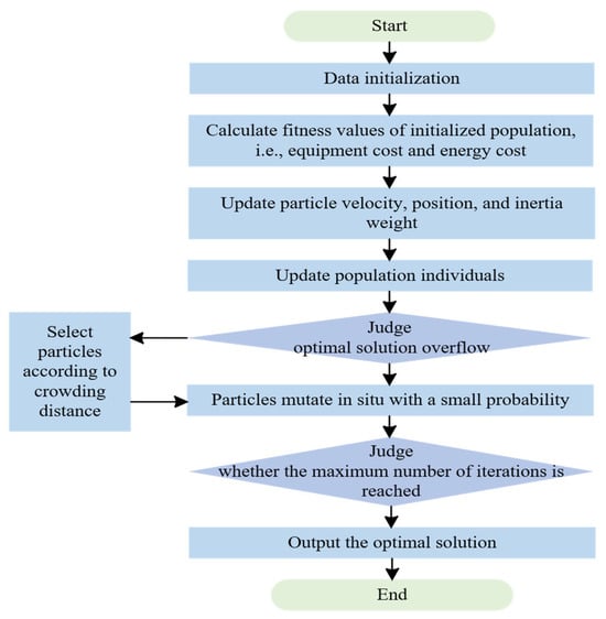
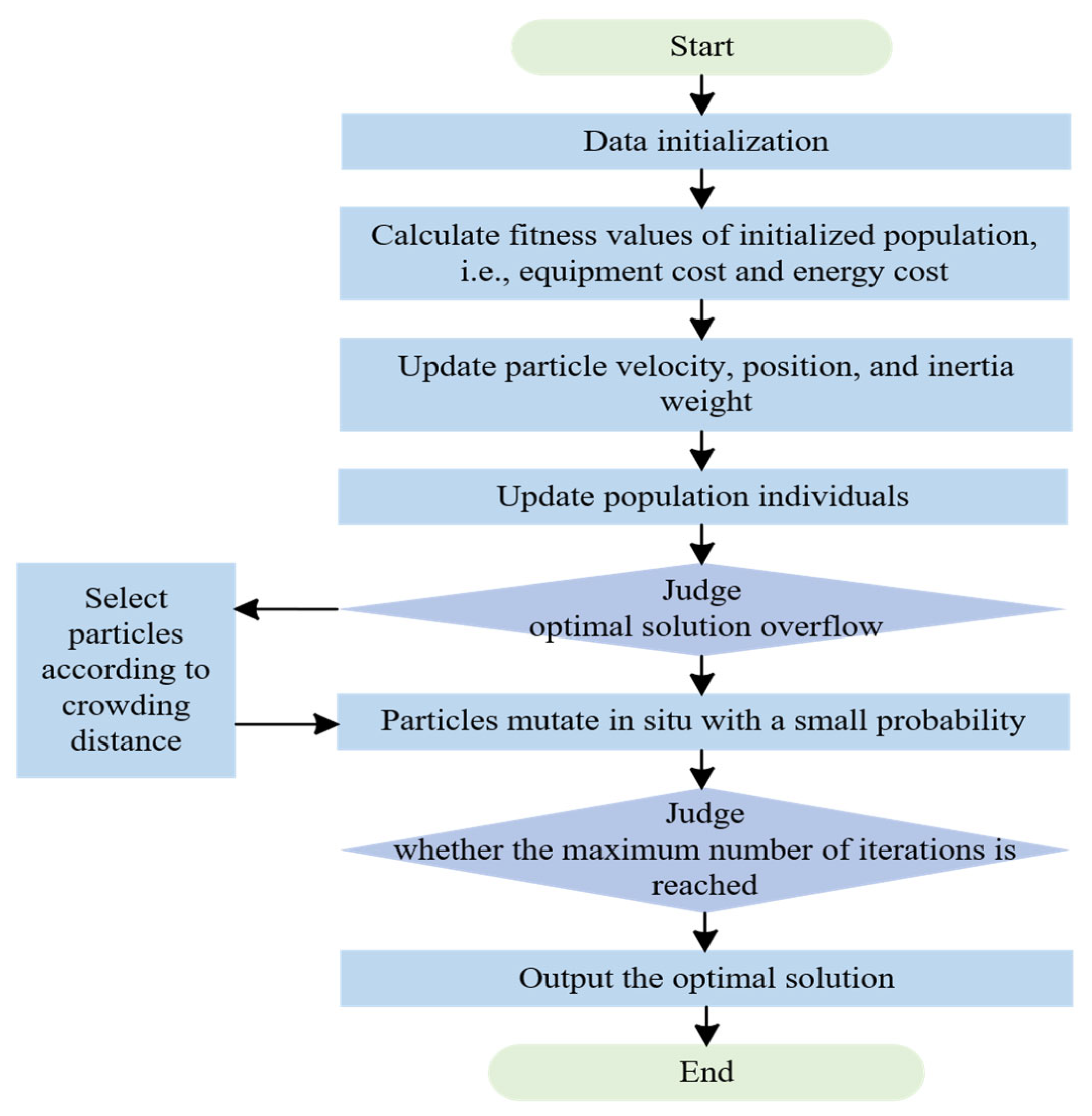
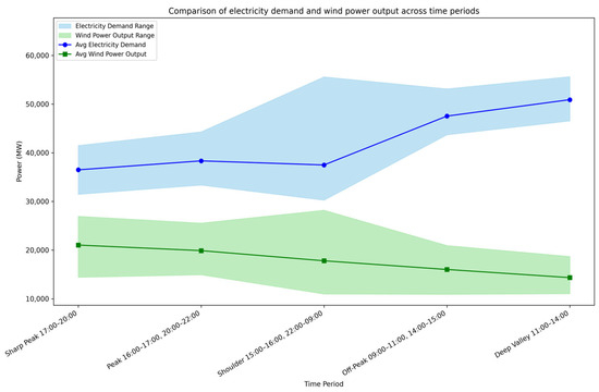
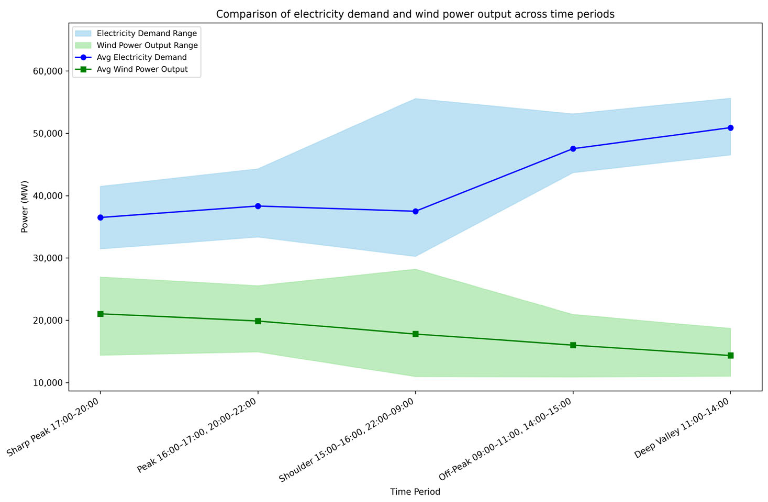
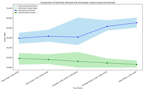
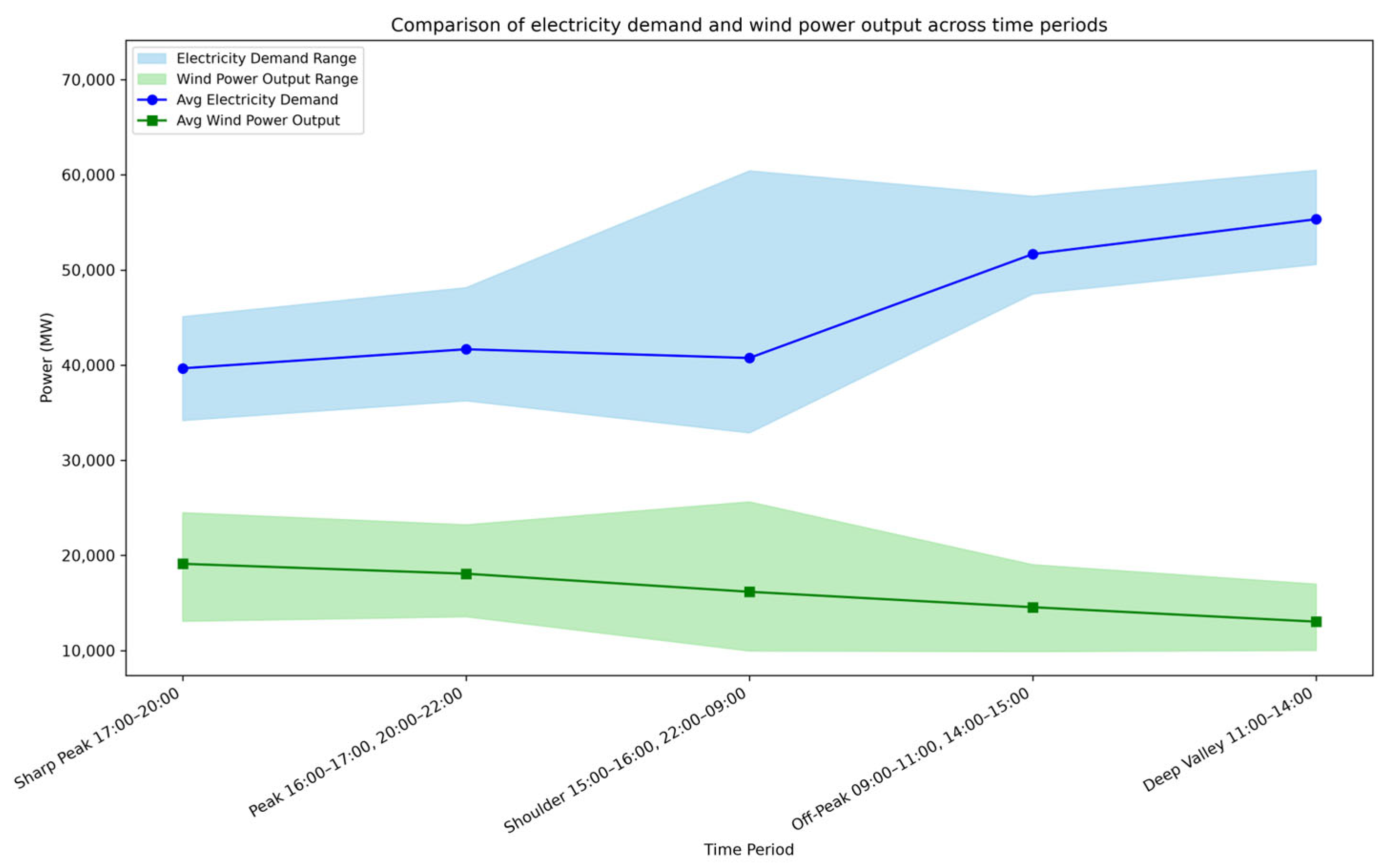
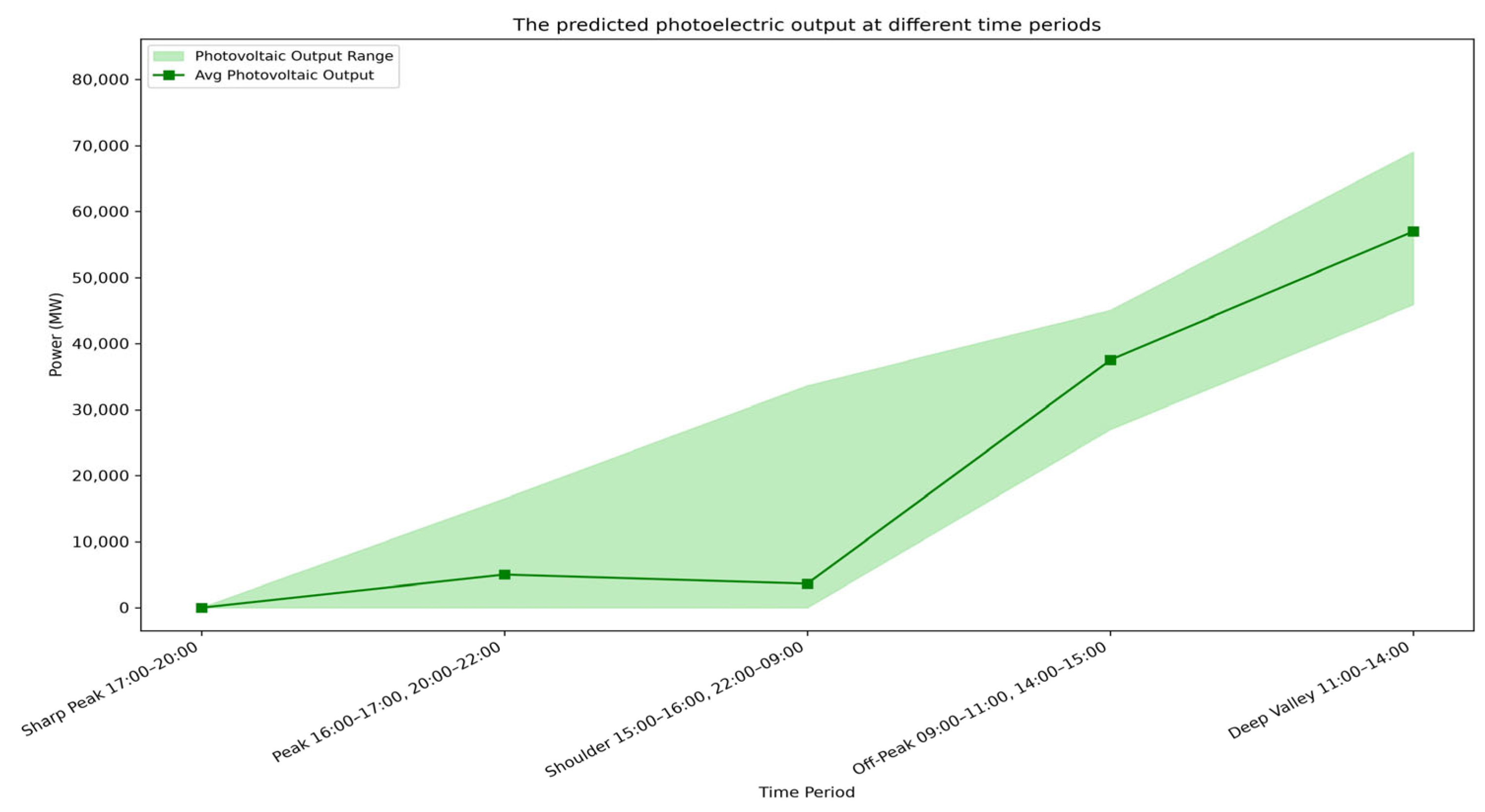
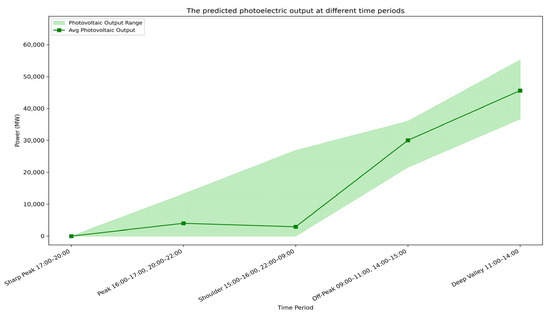
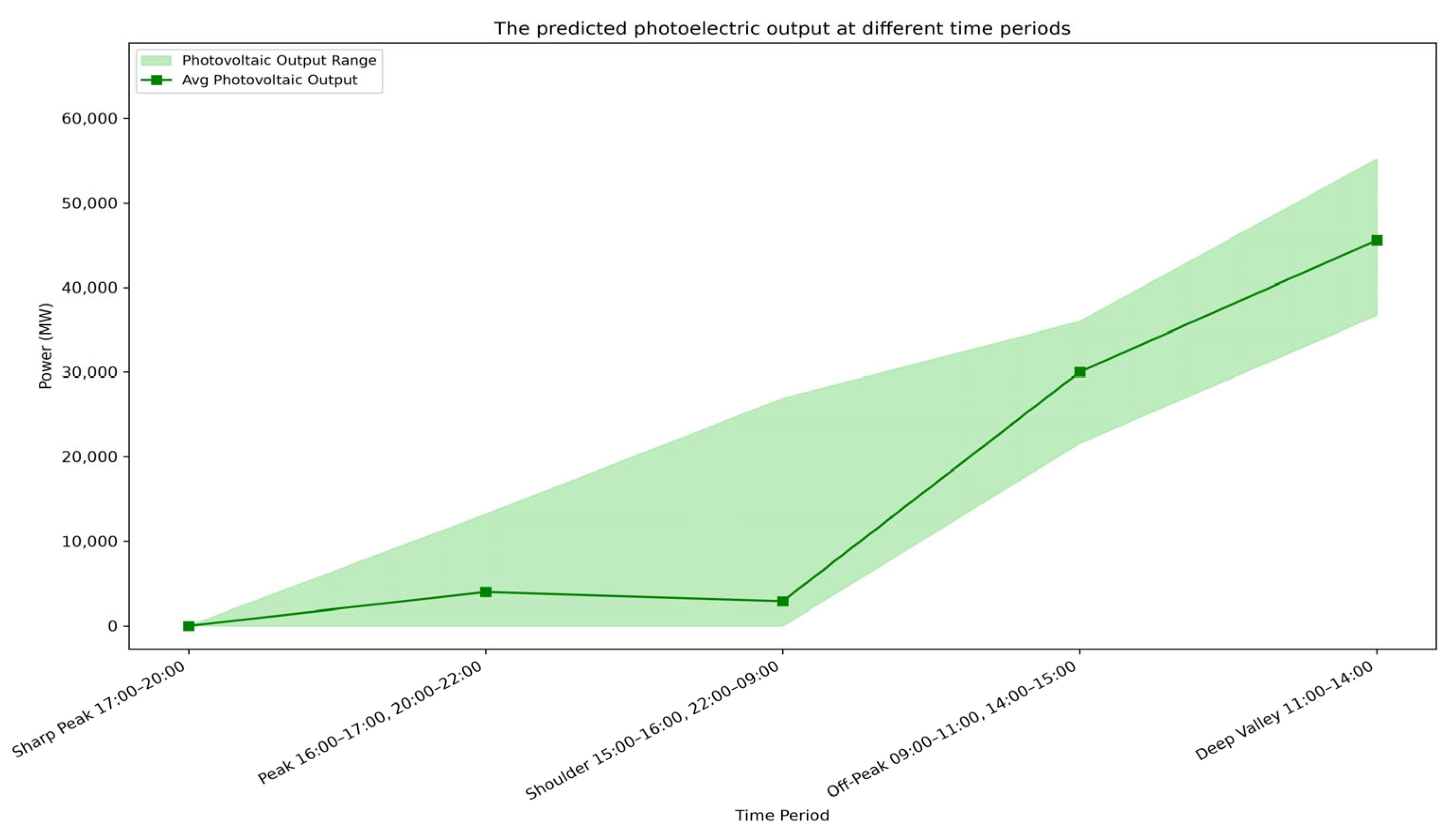
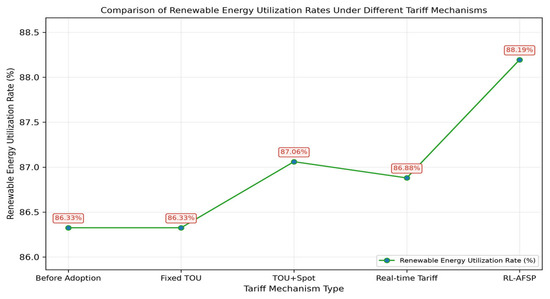
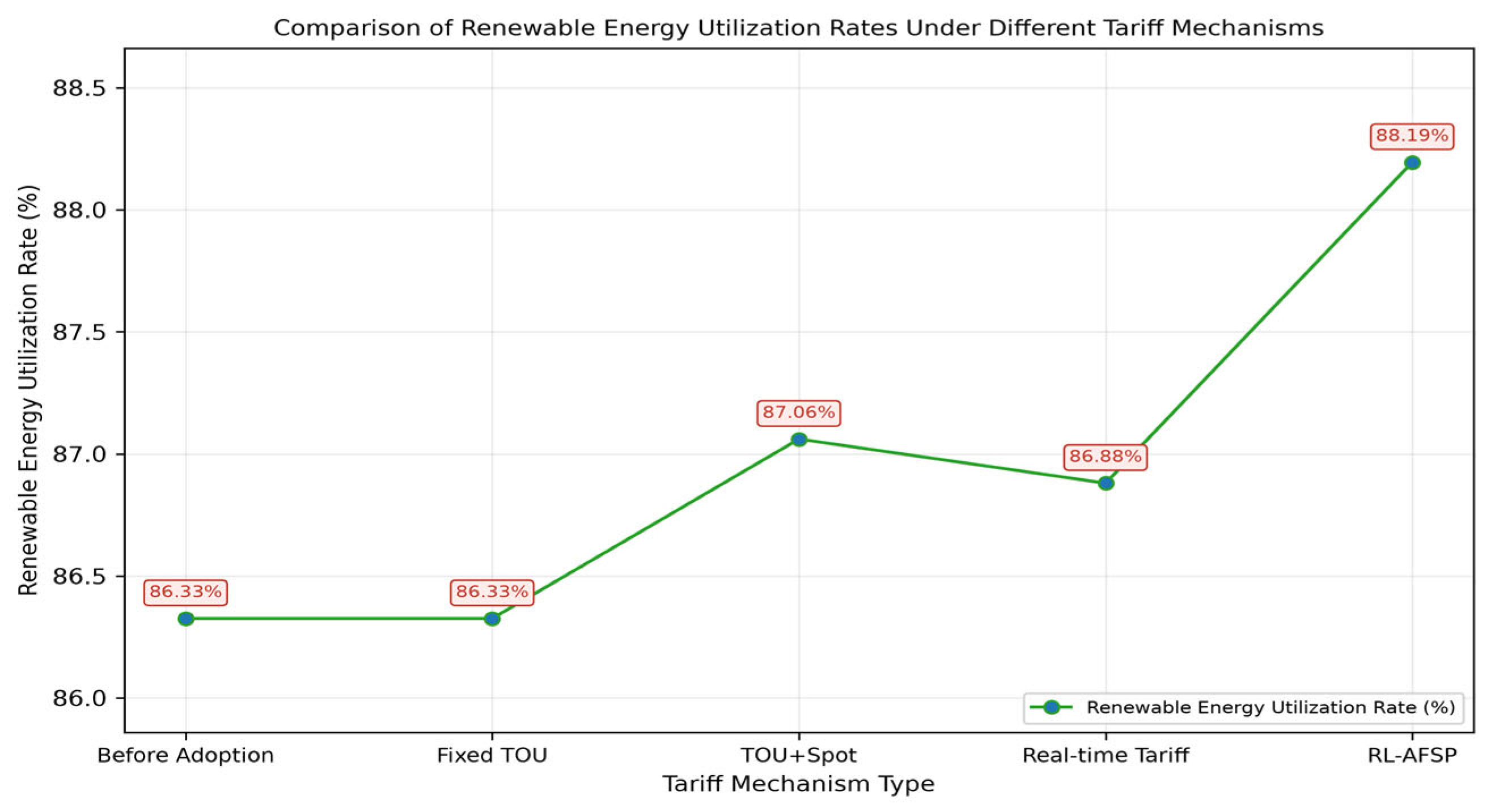
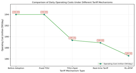
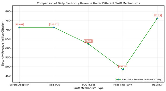
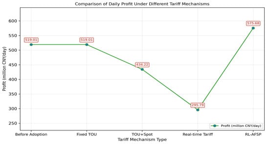
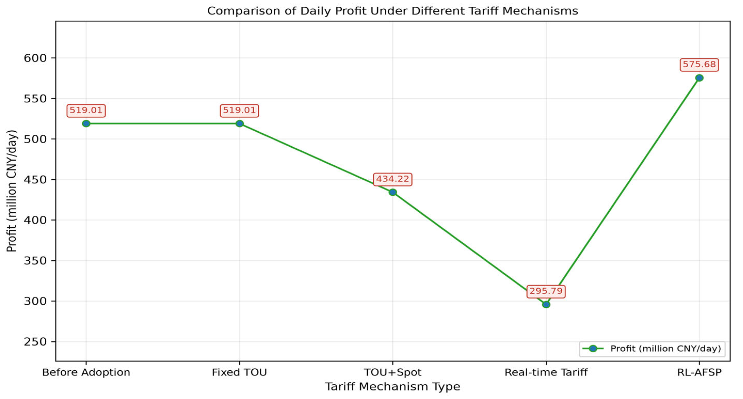
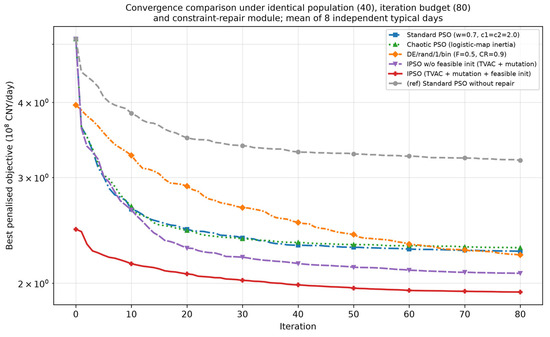
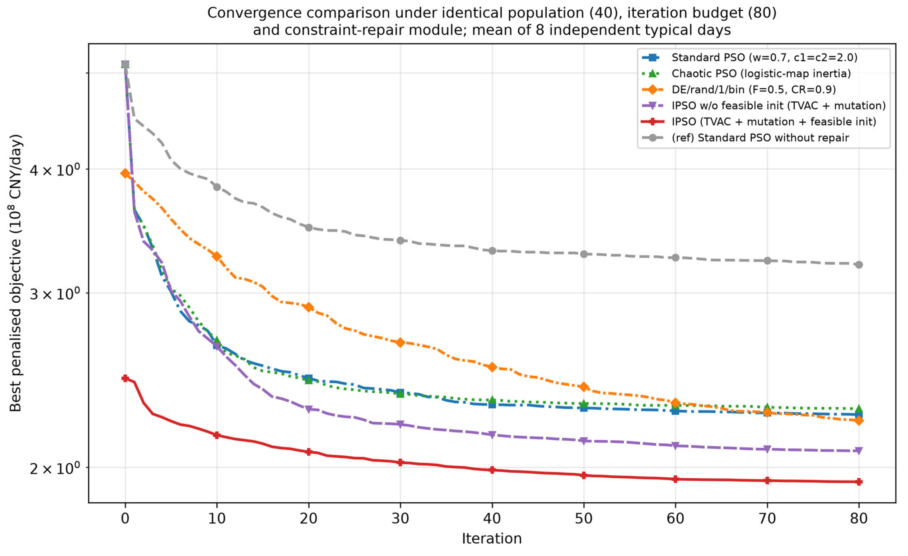

Disclaimer/Publisher’s Note: The statements, opinions and data contained in all publications are solely those of the individual author(s) and contributor(s) and not of MDPI and/or the editor(s). MDPI and/or the editor(s) disclaim responsibility for any injury to people or property resulting from any ideas, methods, instructions or products referred to in the content. |
© 2026 by the authors. Licensee MDPI, Basel, Switzerland. This article is an open access article distributed under the terms and conditions of the Creative Commons Attribution (CC BY) license.