


Abstract
Accurate electricity demand forecasting is essential for improving energy efficiency, operational resilience, and sustainability in modern smart grids. However, existing approaches often treat forecasting and operational control as separate tasks, limiting the effective use of predictive information for sustainable electricity management. This study proposes a forecasting-driven adaptive load-balancing framework that integrates short-term electricity demand forecasting with state-aware operational control within a unified decision-making architecture. A Gradient Boosting Regressor (GBR) predicts future electricity demand, while forecast estimates and uncertainty information guide an adaptive controller designed to improve load distribution during periods of high grid stress. The framework is evaluated using approximately 282,000 half-hourly operational data points from the National Grid Electricity System Operator, covering 2009–2025. On the National Grid ESO forecasting test set, the GBR achieves a mean absolute error of 260.10 MW, a root mean square error of 363.45 MW, a symmetric mean absolute percentage error of 1.079%, and an R2 of 0.9960. These forecasting metrics are calculated from the National Grid ESO demand series, while the IEEE 30-bus system is used exclusively for DC optimal power flow feasibility assessment. Operational evaluations indicate that the proposed adaptive approach reduces peak demand by 27.6%, decreases load variability by 53.22%, and increases the load factor from 0.5777 to 0.7540 compared with a conventional static strategy. Additional temporal validation, uncertainty analysis, scalability tests, sensitivity assessments, and ablation experiments provide further evidence of the framework’s robustness and computational practicality. By enabling demand-responsive load management, the proposed approach offers potential benefits for energy efficiency, grid resilience, and the integration of variable renewable energy resources. These outcomes support sustainable electricity system management, although improvements in renewable energy utilisation, emissions, and environmental performance require direct evaluation. The findings are based on offline historical evaluation; live grid trials, hardware-in-the-loop experiments, and closed-loop operational testing remain necessary before practical deployment can be established.
1. Introduction
The change from conventional electricity systems to modern electricity networks, or from coal to solar and wind generators with interconnected devices, is causing a significant shift in the way utilities operate. The traditional electrical grid was built to serve large-scale generating plants and predictably consume energy. However, the electrical grid is now evolving into a smart grid, which consists of many distributed sources of generation and uses advanced metering infrastructure (AMI) and telecommunications technology to exchange data about electricity usage in real time [1,2].
Although the transition to the smart grid results in a more observable, flexible and energy-efficient grid, it will also create new challenges associated with operational uncertainty due to the intermittency of renewable generation, the stochastic nature of the load, the penetration of electric vehicles, and the variability of decentralised generation. Creating a continuous balance of both the supply and demand of electricity is one of the greatest challenges associated with the operation of smart grids on a large scale today. Near-term supply/demand imbalances can have serious consequences on large electricity networks, including the likelihood of voltage instability and transmission congestion, frequency deviations, increased reserve activation costs, and reduced reliability of operations.
These problems tend to amplify during peak demand or periods of high volatility in renewable generation capacity, where traditional balancing methods tend to be less effective in responding quickly and efficiently [3,4].
Traditional methods for balancing electricity supply and demand include static scheduling, reserve dispatch, and deterministic operational planning; each of these methods was developed with the expectation that the grids would be in a relatively steady state. As such, they are becoming even less effective in responding quickly to the rapidly-changing nature of the current-generation smart grid, particularly in environments that experience dramatic differences in load characteristics over relatively short periods of time.
Maintaining continuous equilibrium between electricity supply and demand therefore remains one of the most critical challenges in contemporary smart-grid operation. In large-scale electricity networks, even short-term imbalances between generation and consumption can trigger voltage instability, transmission congestion, frequency deviations, increased reserve activation costs, and reduced operational reliability. These challenges become particularly severe during peak-demand intervals and periods of volatility in renewable generation, where conventional rule-based balancing strategies often exhibit limited responsiveness and reduced operational efficiency [3,4]. Traditional balancing mechanisms, including static scheduling, reserve dispatch, and deterministic operational planning, were developed primarily for relatively stable grid environments and are increasingly inadequate for highly dynamic smart-grid systems characterised by nonlinear and rapidly fluctuating load conditions [5,6].
Short-term electricity demand forecasting systems have seen substantial enhancements in their prediction capabilities due to recent advances in AI and data-driven energy analytics. Machine learning architectures, ensemble forecasting methodologies, and deep neural networks are now able to effectively predict complex temporal dependencies, seasonal variations, stochastic consumption patterns, and high-frequency load fluctuations in vast amounts of historical operational data [1,7]. Accurate short-term forecasting allows grid operators to work proactively, rather than reactively, to changes in future demand. However, much of the previous research has only viewed forecasting as a singular predictive task, and most of the existing literature has largely focused on the quantitative metrics of forecasting accuracy (e.g., root mean square error (RMSE), mean absolute error (MAE), coefficient of determination ()), with little emphasis placed on how predictive intelligence can directly enhance operational balancing decisions downstream.
Currently available adaptive load-balancing frameworks routinely use synthetic simulations, simplified demand assumptions, or alternative optimisation environments to model the demanding variability and uncertainty of physically existing electricity systems [8]. Therefore, there are few empirical data on which to assess how effectively forecast-informed adaptive balancing techniques would operate under realistic grid conditions. Worst of all, the separation of the methods of forecasting and operating control has resulted in an unfilled area of research within the field of intelligent energy management. It has been observed that while both predictive models and balancing strategies share a high degree of functionality dependence on one another within a practical smart-grid environment, these two items are usually developed separately.
To address these limitations, this study proposes a forecasting-driven adaptive load-balancing framework for intelligent smart-grid optimisation using high-resolution operational data obtained from the National Grid Electricity System Operator (ESO). Unlike conventional approaches that decouple prediction from operational control, the proposed framework establishes a closed-loop predictive–operational architecture in which short-term electricity demand forecasts dynamically inform adaptive balancing decisions in real time. The framework is specifically designed to regulate demand allocation according to predicted grid-stress conditions, thereby reducing peak-load pressure, improving balancing responsiveness, minimising load volatility, and enhancing operational stability under stochastic demand fluctuations.
The proposed framework integrates short-term electricity demand forecasting, uncertainty-aware prediction, nonlinear adaptive balancing, and operational performance evaluation within a unified cyber–physical optimisation architecture. The framework is tested under real grid conditions using about 282,000 half-hourly operational observations from 2009 to 2025, and it is measured based on both forecasting metrics and operational performance indicators. In addition to checking how accurate the predictions are, the method is also analysed based on how much it can lower peak energy use, how well it keeps energy demand steady, how efficiently it balances supply and demand, how well it works with larger systems, how reliable it is when things go wrong, and whether it is easy to set up and use. This provides a full picture of how useful the method is for real smart-grid systems.
The principal contributions of this study are summarised as follows:
- A single framework for adaptive load balancing is created, driven by forecasting, to optimise smart grids intelligently under changing conditions.
- A system is created that uses prediction and control to connect short-term electricity demand forecasts with adjustable balancing control.
- A realistic framework for evaluating performance using high-resolution National Grid ESO operational data is created to test how well systems work under real grid conditions.
- A strategy for assessing operations from multiple angles is suggested, combining statistical forecasting measures with grid performance indicators, allowing for a thorough evaluation of how well predictions and operations are working.
The rest of this paper is arranged as follows. Section 2 examines existing research on smart-grid systems, predicting electricity demand, adjusting balance strategies, and using smart frameworks for managing energy. Section 3 explains the suggested method and the structure of the system. Section 4 covers the results from the experiments and how well the system performed in real use. Finally, Section 5 concludes the study and discusses future research directions.
2. Literature Review
This section looks closely at the latest changes in smart-grid systems that use intelligence, methods for predicting electricity needs in the short term, ways to balance electricity loads adaptively, and systems that optimise operations by making predictions. Much attention is paid to how artificial intelligence used for forecasting is becoming more connected with real-time energy management systems in areas that rely heavily on renewable energy sources. The review brings together key theories and research findings and also points out the main challenges in how methods are designed, performed, and used, leading to the development of the new forecast-based adaptive load-balancing approach.
2.1. Smart Grid Evolution and Intelligent Energy Management
The ongoing transition to greater reliance on renewables, the introduction of distributed energy resources, the deployment of sophisticated metering infrastructure, and the adoption of sophisticated communication technologies have transformed traditional electricity systems into complex interconnected smart grids that combine digital and physical components. Unlike traditional electricity systems that rely primarily on centralised generation and adhere to a fixed set of protocols, contemporary smart grids operate in an environment of fluctuating electricity demand, bidirectional power flow, rising penetration of renewables, and significant operational uncertainty. This requires smart grids to be able to monitor their environment, make accurate forecasts, and make adaptive decisions in real-time [9,10,11,12].
The rapid development of artificial intelligence, machine learning, cloud and edge computing, and distributed optimisation has greatly promoted intelligent energy management in modern power grids. These technologies can help to make precise demand forecasts, integrate renewable energy, optimise generation and consumption [13], perform condition monitoring [14,15], detect anomalies [16] and control the grid in an automated way, thus improving the grid’s flexibility, situational awareness, and reliability [17,18]. In addition, cloud and edge computing can provide scalable computing power to reduce the time of data-intensive computing tasks and make distributed decisions; thus, these technologies have good potential in the field of smart grids.
However, there are still some problems in current intelligent energy management systems. Some methods require massive computation and have limited interpretability, security risks, and are mainly validated on simulation data rather than real-world electricity data [19]. Therefore, it is necessary to design scalable and interpretable intelligent control systems to learn electricity data and make optimal decisions.
2.2. Short-Term Electricity Demand Forecasting
A significant component of smart grid management is forecasting short-term electricity demand, since it has a direct impact on generation planning, reserve allocation, demand response, and other processes. In this regard, demand forecasting contributes to the reduction of balancing costs and the improvement in the overall performance of the system by allowing operators to anticipate load changes and respond to them in a timely manner.
Traditional statistical prediction models, such as ARIMA and regression are proved to be effective enough in the case of rather stable demands. However, they often fail to account for the nonlinear and nonstationary characteristics of modern electricity consumption tendencies [20]. Recently, the need to consider recurrent neural networks, LSTMs, transformers, and ensemble models in electricity demand forecasting has been discussed. These advanced AI methods have been found to be efficient in the case of time series with complex nonlinear behaviour and consumption patterns influenced by the integration of renewable energy sources [21,22].
In recent studies, hybrid prediction systems have been designed to combine the strengths of different approaches and account for varying conditions during the forecasting process [23,24]. At the same time, cloud and edge computing enabled electricity demand forecasting frameworks allowing for reducing computational delays for timely in-time operations [24]. However, the majority of recent studies evaluated the performance of demand forecasting designs in terms of statistical performance prediction metrics, such as the RMSE, MAE, and MAPE. Meanwhile, the improvement in downstream operations, including control and load management, and the overall performance of the grid were rarely considered.
Relevant studies have demonstrated the value of machine learning and deep-learning methods in electricity forecasting. Oprea and Bâra [25] developed a big-data framework using smart-meter and weather-sensor data to compare several machine learning models for short-term residential load forecasting. Bâra and Oprea [26] combined machine learning classifiers for power system imbalance-sign classification with a multivariate stacked LSTM model for predicting electricity imbalance volume. While these studies focus on residential demand and electricity-market imbalance forecasting, respectively, the present study integrates 30 min ahead national demand forecasting with adaptive demand control and operational grid assessment.
2.3. Adaptive Load Balancing and Intelligent Control
With the rapid development of renewable energy, distributed generation and time-varying loads, a promising solution of adaptive load balancing plays a more and more important role in maintaining the stability of the electricity system. Compared to the traditional rule-based scheduling method, the adaptive control strategy not only improves the flexibility of electricity distribution but also enhances system integrity.
The state-of-the-art algorithm for intelligent load balancing is deep reinforcement learning, which can learn decision-making policies from interacting with dynamic operational environments. The latest innovations, including deep Q-networks (DQNs), proximal policy optimisation (PPO), actor–critic frameworks, and multi-agent approaches, have been successfully applied to demand-response management, distributed scheduling, energy storage systems, and smart electricity allocation [27,28,29]. These approaches enable adaptive operational decision making, rapid response to time-varying electricity demands, and coordination of a diverse portfolio of distributed energy resources.
Although the solutions based on reinforcement learning have proved their effectiveness, they currently have several shortcomings, making them less appealing for real-world implementation. First, most of the approaches mentioned require a huge amount of data for training and a significant number of trial-and-error epochs for proper convergence. Second, the majority of them lack transparency, and the process of validation on realistic electricity consumption data is rarely mentioned, thus substantially reducing their practical implementation potential. Therefore, there is a need to design a computationally efficient, interpretable, and reliable algorithm for load balancing that would be trained on the electricity consumption data using the model’s forecasting and control capabilities. Recent metaheuristic approaches include the musical chairs algorithm (MCA), which progressively removes weaker search agents, and the star-nosed mole optimiser (SNMO), which uses multi-sensory searches to balance exploration and exploitation [30,31]. Both could support load scheduling, demand-response allocation and energy optimisation, although their iterative searches increase computational requirements. In contrast, the proposed framework converts GBR forecasts directly into bounded control actions, providing a more interpretable and computationally efficient approach to real-time load balancing.
2.4. Predictive Operational Integration
Recent studies show that smart prediction and control should be treated as two related and interactive functions that must work together to create an integrated energy management system [32,33], rather than separate optimisation problems that require only theoretical solutions. In other words, predictive information can be used to improve decision-making processes in operational planning in order to ensure electricity system flexibility and address emerging challenges associated with renewable energy sources. That is why smart prediction is now used in scheduling, energy management systems, and optimisation processes to improve the performance of distributed energy systems [34].
The development of related technologies, such as cloud and edge computing, the Internet of Things, and distributed intelligence, has made it possible to design modern real-time predictive operational systems [24,29,35]. This is consistent with the need for electricity networks to monitor distributed energy resources and control functions remotely and in real time. At the same time, smart algorithms now allow for faster and more effective optimisation of electricity distribution [36,37]. Despite the above advances, the existing studies still have several limitations. Firstly, the existing methods aim to perform in specific fields, such as microgrids [38], electric-vehicle charging [39], energy storage, and so on. Hence, it is still difficult to apply these methods to the large-scale electricity network. Secondly, most of the existing operational frameworks are based on simulation experiments, which reduces the degree of practicality. Thirdly, a more sophisticated algorithm usually means a more complex structure and difficult implementation, which may not be applied widely. Therefore, there is still a research gap in the building of an integrated framework with an applicable electricity demand forecasting module and real-time load adjustment process to help make decisions in a smart-grid system.
2.5. Comparative Analysis of Existing Frameworks
Table 1 summarises the related work in the areas of intelligent smart-grid management, electricity demand forecasting, adaptive load balancing, and predictive operational optimisation. While the prior work has made substantial progress towards the goals of this study, most of these efforts suffer from similar limitations. Specifically, the prior work addresses electricity demand forecasting and operational control separately, often relies exclusively on simulations for result validation, and rarely provides quantitative confirmation that the proposed approaches operate effectively when deployed on real operational electricity data. The forecasting-driven predictive operational framework described in this study addresses these limitations by combining accurate electricity demand forecasts with real-time adaptive load balancing to enable efficient smart-grid operations.
Table 1.
Comparison of representative AI-driven smart-grid frameworks.
3. Methodology
This section presents the proposed framework for forecasting enabled predictive and operational planning for load balancing in a smart grid. As shown in Figure 1, the proposed framework consists of data acquisition, feature engineering, demand forecasting using machine learning techniques, adaptive load balancing, operational optimisation, and finally the performance evaluation. The proposed framework can be divided into six stages, namely, (i) data acquisition and preprocessing, (ii) exploratory data analysis and validation, (iii) feature engineering, (iv) electricity demand forecasting, (v) adaptive load balancing and operational optimisation, and (vi) performance evaluation and deployment. The framework offers a standard approach that is computationally efficient and can be deployed in real time for smart-grid operation.
Figure 1.
Overview of the proposed forecasting-driven predictive–operational framework.
3.1. Research Design and Predictive Operational Architecture
The framework proposed in this paper focuses on predicting the short-term electricity demand and performing adaptive load balancing based on the prediction results. In other words, electricity demand prediction is used to guide adaptive balancing operations. The overall system is denoted and is defined as the ordered set of its four constituent layers,
where stands for the complete set of the proposed forecasting-driven predictive–operational framework in this study, represents the forecasting layer, stands for the adaptive control layer, refers to the operational optimisation layer, and is the evaluation framework. In other words, is not an extra independent component but the composition of all the , , , and chained together in a closed-loop manner (see Figure 1). Forecast demand is produced on the basis of historical electricity consumption, renewable generation, and temporal features, which are then converted to adaptive control actions and feasible dispatch schedules via the aforementioned layers. In addition, the evaluation layer is responsible for examining forecasting accuracy, operational effectiveness, robustness, and scalability of the proposed approach. Overall, the developed architecture provides a proactive approach to grid management with an interpretable and computationally efficient alternative to reinforcement learning that can be implemented in practice in a timely manner.
3.2. Operational Assumptions
The proposed framework is developed under four practical assumptions that define its operational scope. Let
- : Continuous Demand Monitoring. Electricity demand is recorded every 30 min through advanced metering infrastructure.
- : Feasible Control Actions. Balancing decisions satisfy generation capacity, transmission, and operational constraints.
- : Renewable Generation Range. Renewable generation remains within the historical range represented in the training data.
- : Real-Time Execution. Forecasting and control decisions are completed within each dispatch interval.
These assumptions provide the basis for the forecasting and operational models developed in the following sections.
3.3. Data Preprocessing and Feature Engineering
To capture the temporal and operational characteristics of electricity demand, a unified feature representation combining historical demand, rolling statistics, renewable generation, and cyclical temporal information was constructed.
The feature vector at time step is
where and denote demand lagged by one and two intervals, respectively, and represent the rolling mean and rolling standard deviation of demand computed over the preceding six half-hourly intervals, and denote wind and solar generation at time , and and encode the hour of day as a continuous daily cycle.
This representation captures demand persistence, short-term variability, renewable generation and daily consumption patterns. Temperature, weekday/weekend indicators, public holiday flags and seasonal calendar variables were not included in the present model. This omission limits claims of generalisation across the 2009–2025 period and is acknowledged as an area for future work. The wind and solar generation variables, and , are obtained directly from the National Grid ESO half-hourly system-wide generation-mix records and therefore represent transmission-level, nationally aggregated embedded and metered renewable output rather than site-specific or zonally disaggregated generation. This spatial resolution is consistent with the system-wide nature of the demand series being forecast and is sufficient for capturing the influence of aggregate renewable in-feed on national demand-forecasting error. It is, however, a coarser resolution than would be required for locational or feeder-level analysis, and this limitation is revisited in Section 4 and Section 5. Where zonal or embedded-generation datasets are available, the same feature-engineering pipeline can be extended by replacing the national aggregates and with region-specific vectors without altering the remainder of the framework.
3.4. Forecasting Model Formulation
Electricity demand forecasting is formulated as a supervised nonlinear regression problem,
where is the predicted demand at forecast horizon (measured in half-hourly steps ahead of ), denotes the learned forecasting function parameterised by , and is the engineered feature vector of Equation (1). In all experiments, h = 1, corresponding to one half-hourly interval. Therefore, the reported results represent 30 min ahead forecasting. A new forecast is generated every 30 min using the latest available input features. Several-hours-ahead and day-ahead forecasting were not evaluated in this study. A Gradient Boosting Regressor (GBR) was adopted because it provides high predictive accuracy, computational efficiency, and model interpretability for nonlinear electricity demand forecasting. The function is realised as an additive ensemble built stage-wise,
where is the ensemble prediction after boosting stages, is the regression tree fitted at stage to the pseudo-residuals of , and η ∈ (0,1] is the learning rate that controls the contribution of each successive tree. The final trained model corresponds to after boosting stages, where is the selected number of estimators reported in Table 2. Each successive tree refines the ensemble by minimising prediction error, producing accurate demand forecasts that are supplied directly to the adaptive control layer for operational decision making.
Table 2.
Hyperparameter search space and selected configuration.
3.5. Hyperparameter Configuration and Temporal Validation
Model development followed a strictly chronological protocol to preserve temporal causality and prevent information leakage. Data from 2009–2018 were used for training, while data from 2019–2020 were used for validation and model selection. The final forecasting results were calculated on the independent test window from 17 November to 1 December 2021. Temporal generalisation across the broader dataset was assessed separately using the eight-fold expanding-window walk-forward analysis reported in Section 4.3. No random shuffling was applied at any stage. Figure 2 illustrates the observed and forecast electricity demand over the independent test period, together with the corresponding 80% and 95% prediction intervals.
Figure 2.
Observed and forecast electricity demand with 80% and 95% prediction intervals.
Hyperparameters were optimised using the validation set with early stopping and a patience of 50 boosting iterations to improve generalisation. The search space defining the admissible range for each Gradient Boosting hyperparameter is reported in Table 2, together with the value ultimately selected by the validation procedure. All boundaries were chosen to be wide enough to avoid artificially constraining model capacity while remaining computationally tractable given the dataset size.
Hyperparameter tuning was conducted within the ranges reported in Table 2 using the chronological validation set. Candidate configurations were compared using validation RMSE, and the configuration producing the lowest validation RMSE was fixed before evaluation on the held-out test set. Table 2 reports the search boundaries and final selected configuration. Early stopping was monitored using the predefined chronological validation period of 2019–2020, with training halted after 50 consecutive boosting iterations without improvement in validation RMSE. The held-out test data were not used for early stopping, hyperparameter selection or model configuration. Temporal robustness was further assessed using an expanding-window, walk-forward validation strategy with eight successive folds, reflecting continuous model updating in practical smart-grid operation. The implementation settings are summarised in Table 3. The study used Python 3.11, scikit-learn 1.4 and MATLAB/Simulink R2026a (The MathWorks, Inc., Natick, MA, USA). All preprocessing, normalisation and model-initialisation procedures were applied consistently to ensure reproducibility.
Table 3.
Implementation settings.
3.6. Forecast Uncertainty Quantification
Forecast uncertainty was quantified to evaluate the reliability of electricity demand predictions under varying operating conditions. Let the forecasting residual at time be
where is the observed demand and is the corresponding predicted demand. Assuming calibrated residuals follow an approximately normal distribution, the prediction interval at confidence level is
where is the sample standard deviation of the residuals in Equation (5), and is the Gaussian critical value corresponding to confidence level (e.g., for the 80% interval and for the 95% interval). The resulting intervals quantify forecast confidence and provide additional information for adaptive operational decisions, thereby improving the robustness and reliability of the proposed forecasting-driven framework. Quantile regression and conformal prediction were not implemented in this study and are identified as priorities for future work, together with empirical coverage and interval-width evaluation.
3.7. State-Aware Adaptive Load-Balancing Framework
The proposed adaptive load-balancing framework constitutes the primary contribution of this study by directly coupling electricity demand forecasting with operational control. Instead of treating forecasting as an independent task, predicted demand is used to determine adaptive balancing actions under changing grid conditions.
The grid state at time is defined as
where is the observed demand, is the forecast demand, and is the standardised grid-stress index defined in Equation (8). The two remaining state components describe complementary operating conditions used to contextualise the stress index: is the normalised forecast uncertainty ratio, obtained from the residual standard deviation of Equation (6) relative to the current forecast, and is the forecast renewable in-feed ratio, i.e., the proportion of forecast demand expected to be met by wind and solar generation. The forecast uncertainty ratio is incorporated directly into the control law through the factor in Equations (11) and (12). As the forecast uncertainty increases, this factor reduces the influence of the forecast-based stress index and produces a more conservative curtailment response. The renewable in-feed ratio is retained for monitoring and post hoc analysis.
Grid stress is computed as
where and denote the historical mean and standard deviation of electricity demand over the training period.
Peak operating conditions are identified using:
where is the empirical ninetieth percentile of the demand distribution.
To avoid ambiguity between the maximum permissible demand reduction and the bounds placed on the regulation multiplier, two distinct symbols are used. Let denote the fraction of demand curtailed at time , where is the maximum permissible demand reduction (30%). The regulation multiplier is then
so that corresponds to no intervention and corresponds to the maximum permitted intervention.
During periods of elevated grid stress (), the curtailment fraction is
and under normal operating conditions (), a smaller precautionary curtailment is applied,
The regulation multiplier is bounded as
where and , i.e., . This ensures that the constraint is internally consistent: the multiplier can never fall below 0.70 (equivalently, curtailment can never exceed 30%) and never exceeds 1.00 (equivalently, curtailment is never negative).
The regulated demand is obtained as
allowing the balancing intensity to increase progressively with forecast grid stress while the floor guarantees that the maximum permissible curtailment is never exceeded.
To ensure operational stability, consecutive control actions satisfy
where is the applied curtailment action and is the maximum allowable control variation between consecutive dispatch intervals, preventing abrupt or oscillatory regulation.
The resulting controller provides an interpretable and computationally efficient alternative to reinforcement learning while remaining suitable for real-time smart-grid deployment.
Physical Realisation of the Adaptive Curtailment Signal
The curtailment fraction produced by the controller is a dimensionless operational set-point rather than a direct instruction to a single physical device; it must be translated into concrete actions by the demand-side layer of the grid before it has any physical effect. In the proposed framework, this translation is achieved through three complementary, commercially established mechanisms, which are combined so that the aggregate curtailment delivered matches MW at each dispatch interval:
- Contracted demand response. Aggregated flexible industrial and commercial loads, participating through demand-response service providers, receive a dispatch instruction proportional to and temporarily reduce or shift consumption (e.g., pausing non-critical processes, adjusting HVAC set-points), consistent with existing balancing mechanisms and demand-turn-up/turn-down products already operated by system operators.
- Smart appliance and electric-vehicle charging deferral. Where AMI-connected smart appliances, heat pumps, and electric-vehicle chargers are enrolled in a managed-charging programme, the curtailment signal is converted into a temporary reduction of the maximum charging/consumption rate, deferring non-time-critical load without altering the total energy delivered over the charging window.
- Battery energy storage and price-based signalling. Grid-scale and behind-the-meter storage assets discharge in proportion to during peak-stress intervals, while a residual portion of is delivered through short-horizon dynamic-pricing signals to price-responsive consumers.
These resource classes are not modelled separately, and the analysis does not explicitly represent response rates, customer participation, minimum operating requirements, rebound effects or contractual limitations. The reported curtailment therefore assumes that sufficient flexible capacity is available at each dispatch interval. Resource-level participation, flexibility and rebound data are not available in the National Grid dataset. Accordingly, the analysis assumes delivery of the aggregate curtailment request and does not impose separate participation rates, minimum service limits or rebound profiles. The controller operates at a 30 min dispatch interval, and response delays of 1, 5 and 15 min are evaluated in Section 4.9.4. The reported curtailment should therefore be interpreted as a conditional system-level estimate rather than demonstrated resource-level capability. The rate-limiting constraint of Equation (15) is what makes this translation practical: because the controller output changes gradually between dispatch intervals, aggregated resources can be recruited using existing minutes-to-hours-ahead dispatch instructions rather than requiring sub-second automatic control, which keeps the mechanism compatible with current demand-response and battery-dispatch operating procedures. The relative contribution of each mechanism to a given is a commercial-allocation decision made by the aggregator/operator layer and is outside the scope of the forecasting and control architecture proposed here; the present study evaluates the aggregate MW-level effect of on system demand, consistent with the operational-level, rather than device-level, scope stated in Assumption .
3.8. Operational Dispatch Optimisation
The regulated demand is converted into feasible generation schedules through an operational dispatch optimisation layer. To support computational efficiency and real-time implementation, dispatch is formulated using the linearised DC optimal power flow (DC-OPF) model, which provides a practical balance between computational cost and operational accuracy.
The optimisation problem is
subject to
where is the marginal generation cost of unit (£/MWh), is the dispatched output of unit , is the regulated demand of Equation (14) that the dispatch layer must meet at interval , and is the maximum generation capacity of unit . The objective in Equation (16) is the total system generation cost, i.e., the sum over all units of the marginal cost multiplied by the dispatched output ; minimising it subject to Equation (17) yields an economically efficient dispatch that exactly meets the regulated demand while respecting each unit’s capacity limit.
Because the National Grid ESO operational dataset used in this study reports system-wide half-hourly demand and generation-mix quantities rather than bus-level telemetry, the DC-OPF layer is evaluated on a standardised, publicly documented reduced network representation rather than on a bespoke or undisclosed topology. Specifically, dispatch feasibility was assessed using the standard IEEE 30-Bus Reliability Test System [42,43] (6 generator buses, 41 branches), whose generator cost coefficients , branch reactances , and line thermal ratings were taken directly from the published test-case data distributed with MATPOWER version 8.1 [43].
Because the raw IEEE 30-bus case represents a network with an installed capacity far smaller than the Great Britain system, its generation and thermal capacity parameters were rescaled prior to use. A single scaling factor
was computed, where is the observed National Grid ESO peak demand over the evaluation window and is the total installed generation capacity of the unscaled IEEE 30-bus case. Every generator capacity limit and every branch thermal rating in the test case were then multiplied by , i.e.,
while the generator cost coefficients and the per-unit branch reactances were left unscaled. Applying a single multiplicative factor uniformly across all generators and branches preserves the relative distribution of generation cost and transmission thermal headroom across the network (i.e., the merit order and the relative tightness of each line remain unchanged) while ensuring that the absolute scale of the network matches realistic Great Britain operating conditions, so that the regulated demand series produced by the adaptive controller is dispatch-feasible at a realistic operating scale. Branch thermal limits are enforced as
for each line , where and are the voltage phase angles at buses and , using the standard DC power flow (line-susceptance) approximation. This substitution is reported explicitly as a limitation: it demonstrates that the regulated demand trajectory is feasible under a realistic, reproducible, and citable network topology, but it is not a bus-level validation against the real Great Britain transmission network, whose commercially sensitive topology, admittance, and thermal-limit data are not published by the National Grid ESO at the resolution required for OPF studies. Section 5 identifies collaboration with a transmission operator to obtain the real network model as a direction for future work.
DC-OPF is used solely as a static dispatch-feasibility assessment. It represents power balance, generator-capacity limits and branch thermal constraints but does not include generator ramp rates, minimum generation levels, reserves, start-up costs, network losses, voltage-magnitude and reactive-power constraints, storage state of charge or detailed demand-response constraints. The results should therefore not be interpreted as complete validation of real-world grid operation. Because DC-OPF receives the regulated demand after the controller has applied curtailment, it optimises generation dispatch only and does not independently select loads for curtailment or coordinate flexible resources.
3.9. Performance Evaluation Framework
The proposed framework was evaluated from both the predictive and operational perspectives. Unlike conventional forecasting studies that focus only on prediction accuracy, the evaluation jointly examines forecasting performance, load-balancing effectiveness, computational robustness, and statistical significance. Forecasting accuracy was measured using the mean absolute error (MAE), root mean squared error (RMSE), symmetric mean absolute percentage error (SMAPE), and the coefficient of determination ().
Operational performance was evaluated using peak reduction
load-variance reduction
and balancing efficiency
where denotes the demand series obtained under conventional static (uncontrolled) operation, used here as the operational baseline against which the regulated series is compared. Statistical significance was assessed using the Diebold–Mariano (DM) test with heteroskedasticity- and autocorrelation-consistent variance estimation, while uncertainty was quantified through a moving-block bootstrap with 1000 resamples. Because standard independent and identically distributed bootstrap resampling destroys the temporal autocorrelation inherent to half-hourly electricity demand, blocks of contiguous observations, rather than individual half-hourly points, were resampled with replacement. A block length of 48 consecutive half-hourly observations (24 h) was selected to preserve the dominant diurnal autocorrelation structure identified during exploratory analysis; sensitivity checks using block lengths of 24 (12 h) and 336 (7 days) produced confidence intervals within 3% of those reported, confirming that the results are not sensitive to the precise block-length choice. Together, these measures provide a comprehensive assessment of forecasting accuracy, operational performance, robustness, and statistical reliability within a unified evaluation framework.
4. Results and Discussion
This section provides an in-depth examination of the forecasting-informed adaptive load-balancing approach based on the data provided by National Grid ESO. The experiments will concern the accuracy of the forecasting model, a comparison of the obtained results to state-of-the-art models, temporal generalisability, uncertainty, the contribution of the individual components, computational complexity, the impact of selected disturbances on the performance of the approach, sensitivity analysis, the influence on the economy and consumers, and the readiness of the approach for practical applications. In general, the experiments will focus on the accuracy of the forecasting model and the quality of the resulting decisions concerning the operation of the grid.
4.1. Short-Term Electricity Demand Forecasting Performance
The forecasting accuracy of the various models was first evaluated on an independent test period covering 17 November to 1 December 2021. The resulting performance metrics are reported in Table 4.
Table 4.
Forecasting performance summary.
As shown in Table 4, the Gradient Boosting Regressor had outstanding performance across all metrics with a mean absolute error of 260.10 MW, root mean squared error of 363.45 MW, symmetric mean absolute percentage error of just 1.079%, and a coefficient of determination of 0.9960. Notably, given the overall system demand of approximately 24,571 MW, these errors are relatively small, suggesting that the model is generating accurate estimates of the electricity demand across the different loading conditions. The high coefficient of determination suggests that the learning architecture has managed to capture the majority of the dominant patterns that shape electricity consumption, including the characteristic daily and weekly demand cycles, as well as more transient variations in the load. This demonstrates the combined effectiveness of the engineered temporal features, renewable generation variables, rolling statistics, and nonlinear ensemble learning in electricity forecasting.
Figure 2 illustrates the agreement between the observed and predicted demand profiles throughout the evaluation period, together with the corresponding 80% and 95% prediction intervals of Equation (6). The predicted trajectory closely follows the measured demand over the test horizon and reproduces the gradual evolution of the load and periods of high electricity consumption with no apparent divergence, as can be seen in Figure 2. The prediction bands are also fairly consistent over time, providing stable estimates of the uncertainty while staying close to the measured demand. These results therefore provide a solid basis for the adaptive operational strategy that will be analysed in the following sections.
4.2. Comparative Performance Evaluation
The forecasting comparison is limited to the persistence and moving-average baselines. These benchmarks assess whether the GBR provides improvement over simple historical extrapolation but do not constitute a comprehensive comparison with advanced ensemble or deep-learning models. Accordingly, the results support superiority only over the evaluated baselines and should not be interpreted as demonstrating that GBR outperforms XGBoost, LightGBM, Random Forest or modern time-series models. A broader comparison with these methods remains an important direction for future work. The comparison results are summarised in Table 5.
Table 5.
Comparative forecasting performance on the test dataset.
On all metrics, the Gradient Boosting Regressor clearly outperformed the benchmark approaches. Compared to the persistence model, the mean absolute error and the root mean squared error were reduced by more than 57%, while the symmetric mean absolute percentage error was decreased from 2.57% to 1.08%. Such an improvement highlights the benefits of the considered approach over a naive model that only accounts for the short-term temporal continuity in the data. The differences between the method’s performance and the moving-average model are even more significant. While the latter type of approach is able to capture the slow-varying patterns in the demand data, it is not capable of reflecting the rapid changes in electricity consumption, since such variations get smoothed out in the calculation. However, the proposed solution with engineered temporal features, renewable generation data, rolling statistics, and a nonlinear model ensemble is able to reflect both gradual transformations in the demand profile and sudden variations in electricity consumption, which leads to significantly better forecasts. Finally, Table 6 provides a qualitative comparison of the method with the relevant publications on the topic of electricity demand forecasting. Since different papers cover varying aspects of the problem and utilise different evaluation criteria, quantitative comparison between the different approaches is not possible.
Table 6.
Comparison with representative electricity demand forecasting studies.
The studies summarised in Table 6 are primarily concerned with improving the forecasting accuracy, with performance measured exclusively in terms of the accuracy of prediction. The current work goes beyond this paradigm by combining demand forecasting with adaptive load balancing within one operational system. In this setting, the demand forecasts are not an end in and of themselves but are used as inputs for operational control, whereby predicted demand informs load balancing in an evolving grid state. This approach has the potential to widen the scope of electricity demand forecasting from the purely predictive to the operational control space, enabling new opportunities for smart-grid management.
4.3. Temporal Generalisation
While the previous experiments evaluate the predictive accuracy on an independent test set, real-world applications demand reliable performance for varying operating conditions. In order to assess temporal generalisation, a walk-forward scheme was applied that expands the training window while preserving the chronological ordering of the observations (thereby avoiding information leakage). The forecasting outcomes over the eight validation folds are provided in Table 7.
Table 7.
Walk-forward validation results.
The eight folds yielded RMSE values of 369.99–670.39 MW, with a mean of 503.54 ± 103.02 MW, a coefficient of variation of 20.46% and a 95% confidence interval for the mean of 417.40–589.68 MW. This variation indicates temporal non-stationarity across the extended multi-season fold periods, although the contribution of individual factors cannot be isolated from the available features. The final-test RMSE of 363.45 MW was calculated only for 17 November–1 December 2021, whereas each walk-forward fold contains 31,348 observations covering a broader range of operating conditions. The two results are therefore not directly comparable, and claims of uniformly stable performance have been removed.
Figure 3.
Fold-wise RMSE obtained using expanding-window, walk-forward validation. Numbers above the bars show RMSE rounded to the nearest MW; the dashed line indicates the mean RMSE (503.54 MW).
The final-test and walk-forward RMSE results are not directly comparable because they cover evaluation periods of different lengths and operating conditions. The variation across the eight folds indicates temporal variability rather than uniformly stable forecasting performance.
4.4. Residual and Uncertainty Analysis
In addition to point forecasts, reliable measures of the uncertainty associated with each prediction are required for operational deployment. Residual diagnostics were therefore performed to investigate systematic bias in predictions, the variability of prediction residuals and the calibration of the estimated prediction intervals. The principal diagnostic statistics are summarised in Table 8.
Table 8.
Residual diagnostic and uncertainty summary.
The residual statistics confirm that the mean bias is small—just MW compared to the total demand range. This implies that errors are small and centred on zero: the forecast is consistently neither over- nor under-estimating the demand. The prediction intervals in Equation (6) are based on a single residual standard deviation and should therefore be interpreted as approximate Gaussian uncertainty bands rather than empirically calibrated intervals. Their half-widths are 462.37 MW and 706.90 MW at the 80% and 95% levels, respectively, and remain constant throughout the test period. The calibration factor of 1.015 is reported as a descriptive measure and is not treated as proof of statistical reliability. Empirical coverage, calibration plots and separate peak and off-peak coverage were not evaluated and therefore remain limitations of the present uncertainty analysis.
Figure 4 presents the residual distribution together with the temporal evolution of the forecasting errors; most residuals are distributed close to zero, with only occasional large residuals occurring during high demand periods. This is expected due to the higher uncertainty associated with rapidly varying demand profiles, thus demonstrating that the forecast error is primarily due to demand variability and not systematic modelling errors. The accurate quantification of uncertainty is critical for the forecasting-centric operational paradigm developed in this study. As adaptive load-balancing mechanisms respond to both the forecast demand and its uncertainty through the uncertainty ratio defined in Equation (7), calibrated prediction intervals empower the controller to take larger steps in response to higher confidence forecasts while being more conservative in the face of growing forecast uncertainty, thus ensuring reliability while avoiding unnecessary interventions.
Figure 4.
Residual distribution and temporal evolution of forecasting errors over the evaluation period. Dashed grey lines indicate zero residual. The horizontal dotted black lines mark ±1.96 residual standard deviations (approximately ±706.90 MW).
4.5. Adaptive Load Balancing Performance
Having established the predictive accuracy, temporal stability and uncertainty calibration of the model, the subsequent stage of the evaluation considers the implications of forecast information on operational decision making. The aforementioned adaptive load-balancing strategy described in Section 3 was therefore driven by the predicted demand profiles to evaluate the extent to which it was effective under realistic operating conditions of the grid. Instead of operating with uniform demand regulation, the controller was able to adjust the level of intervention depending on the current system state, leaving normal operations mostly unaffected but operating with increased intensity during stressful periods. The principal operating parameters adopted by the controller are summarised in Table 9.
Table 9.
Adaptive load-balancing configuration parameters.
Figure 5 compares the resulting demand profiles obtained under conventional static operation and the adaptive regulation strategy.
Figure 5.
Static and adaptive load balancing across the evaluation period.
As shown in Figure 5, the control action takes place mostly around the peaks of the system load while following the reference profile closely otherwise, which shows that the control action is taken only when it is needed to reduce the peaks. The corresponding operational performance is reported in Table 10.
Table 10.
Operational performance of the static and adaptive frameworks.
The adaptive strategy decreased the maximum system demand by 27.6%, reducing the network peak from 42,458 MW to 30,732 MW and demand variance by 53.22%, which suggests significantly smoother load profiles. The load factor increased from 0.5777 to 0.7540, suggesting a more uniform use of the generation and transmission resources of the network. The controller thus achieves higher utilisation by making demand more uniform, without the need for extra generation resources. While the adaptive strategy created a larger tracking error than the static baseline, it is the result of actively managing demand, not poor prediction. The controller is designed to actively change the demand trajectory to lower peak load and make the demand less variable. The tracking error must therefore be seen in the context of the benefits of load shaping, rather than as a cost. Statistical tests using the Diebold–Mariano test confirm that the improvements are significant under heteroskedasticity- and autocorrelation-consistent variance estimation (). The results suggest that the value of accurate demand forecasts can be significantly improved by supplementing them with adaptive operation, turning forecast uncertainty into operational gains in peak shaving, load shaping and utilisation.
4.6. Comparison with Alternative Control Strategies
To quantify the specific contribution of the proposed state-aware controller relative to other operational control paradigms, the forecasting model was held fixed and coupled in turn with three alternative control strategies: (i) a fixed-threshold, rule-based controller that applies a constant curtailment whenever forecast demand is greater than ; (ii) a classical feedback proportional-integral-derivative (PID) controller, tuned via Ziegler–Nichols relay tuning to drive demand towards the historical mean; and (iii) a short-horizon model predictive control (MPC) scheme, using a two-hour receding prediction horizon and the same GBR forecasts as the proposed controller. All four controllers were assessed on the same test period and definition of regulated demand as used elsewhere in this study. The results are summarised in Table 11.
Table 11.
Controller comparison: Peak and variance reduction (%), load is a factor, and latency is in ms.
The fixed-threshold and PID controllers achieve meaningfully smaller reductions in peak and variance than the proposed controller since they do not adapt their intervention intensity to the magnitude of the forecast grid stress: the former applies the same level of curtailment regardless of how far demand exceeds , while the latter’s proportional-derivative terms result in visible control oscillation (repeated over- and under-correction) around the demand target, which is undesirable for aggregated demand-response dispatch. The MPC scheme performs close to the proposed controller since it also uses the GBR forecasts and the same regulated demand objective, demonstrating that most of the possible operational improvement accrues from combining accurate forecasting with any anticipatory controller. However, the MPC requires solving a constrained quadratic program at each dispatch interval, increasing the inference latency by roughly two orders of magnitude relative to the closed-form proposed controller (38.6 ms versus <0.1 ms), an amount that is only material at very large numbers of simultaneously controlled aggregation points or very short dispatch intervals. The proposed state-aware controller thus achieves at least as good operational performance as MPC, only with the low computational cost and interpretability of a rule-based scheme—the specific trade-off this paper targets for large-scale, low-latency deployment.
To confirm that the reported differences in Table 11 are not attributable to sampling noise, each alternative controller’s regulated demand series was compared against the proposed controller’s regulated demand series using the same Diebold–Mariano procedure with heteroskedasticity- and autocorrelation-consistent variance estimation described in Section 3, and 95% confidence intervals for the difference in variance reduction were obtained from the moving-block bootstrap (1000 resamples, 48-step block length). The results are reported in Table 12.
Table 12.
Statistical significance of the proposed controller versus alternatives.
The proposed controller is statistically significantly better than all alternatives at the 5% level, including MPC (), although the effect size compared to MPC is small (0.6–2.6 percentage points of variance reduction) and, as mentioned above, comes with a roughly decrease in per-interval inference latency. The much larger, highly significant improvements versus the fixed-threshold and PID controllers ( in both cases) demonstrate that this state-aware, forecast-conditioned regulation law is responsible for most of the operating gain and not simply the inclusion of any feedback.
4.7. Economic and Consumer Impact Analysis
Beyond technical performance, the practical value of the proposed framework depends on its economic implications for system operators and its impact on end consumers. This subsection provides an illustrative, order-of-magnitude assessment; it is not a substitute for a full market-level cost–benefit study, which would require confidential balancing-cost and tariff data not available to the authors.
4.7.1. System-Level Economic Impact
Reserve and balancing costs on the GB system are strongly correlated with peak demand and short-term demand volatility, since both drive the activation of increasingly expensive reserve and reserve-of-last-resort generation. To make this relationship explicit, the avoided balancing cost over an evaluation window of dispatch intervals is estimated as
where and are, respectively, the static demand and the regulated demand of Equation (14) at interval , h is the half-hourly dispatch interval, and is a representative unit balancing-services cost, expressed in £/MWh, applied to the total avoided peak/reserve exposure (i.e., is the product of the unit cost and the cumulative avoided energy volume). A monetary value is not assigned in this study because the analysis does not identify which balancing mechanism actions or reserve products would have been displaced during each settlement period. Balancing costs vary over time according to system conditions, the service procured and the applicable price [45]. Consequently, curtailed demand cannot be converted directly into an equivalent avoided system cost. Equation (24) is therefore retained only as a conceptual relationship. A market-level valuation would require settlement-period price and activation data together with demand-response participation and implementation costs.
4.7.2. Consumer Impact
Service windows constrain smart appliances and EV charging, while power and state-of-charge limits constrain storage, and process and contractual limits constrain flexible loads. Because these resource-specific constraints are not modelled separately, the consumer-impact results are qualitative and should not be interpreted as uniform across participants. For consumers exposed to dynamic-pricing signals, the reduction in peak and variance directly reduces the frequency and severity of high-price balancing events, which is generally associated with lower average bills for flexible consumers [46] but requires opt-in transparency and safeguards for vulnerable or inflexible consumers who cannot shift consumption. An equity consideration therefore follows directly from the mechanism: because participation in demand response and dynamic pricing is not uniform across income groups, the framework should be paired with protections (e.g., an opt-out default, or exclusion of essential heating/medical loads from ) to avoid disproportionately shifting curtailment onto consumers least able to respond. This is flagged as an important deployment consideration rather than a solved problem within the scope of the present forecasting and control study.
4.8. Ablation Study
To quantify the contribution of each constituent component, an ablation study was performed using five progressively enhanced model configurations evaluated under identical training partitions, testing data, hyperparameter settings, and evaluation procedures. This experimental design isolates the incremental effect of each modelling component while ensuring that observed performance differences arise solely from architectural modifications. The evaluated configurations comprise: (i) persistence forecasting with static dispatch (M0), (ii) Gradient Boosting Regression using only lagged demand features (M1), (iii) the complete forecasting model incorporating engineered temporal and renewable generation features without adaptive control (M2), (iv) forecasting combined with fixed-threshold regulation (M3), and (v) the complete forecasting-driven adaptive load-balancing framework (M4). The corresponding results are presented in Table 13.
Table 13.
Ablation study of the proposed framework.
The progressive evolution from M0 to M4 reveals a clear accumulation of predictive and operational capability as successive framework components are introduced. Replacing persistence forecasting with Gradient Boosting Regression based solely on autoregressive demand information (M1) substantially reduces the forecasting error, illustrating the benefit of nonlinear machine learning for modelling electricity demand dynamics. Extending the feature representation through temporal descriptors, renewable generation variables, and rolling statistical characteristics (M2) produces a further improvement, reducing the mean absolute error to 260.10 MW while increasing the coefficient of determination to 0.9960. These results demonstrate that accurate demand forecasting depends not only on model complexity but also on informative feature representation capable of describing the temporal evolution of electricity consumption.
Introducing operational control through a fixed-threshold strategy (M3) leaves the forecasting performance unchanged while delivering measurable improvements in grid operation, including an 18.3% reduction in peak demand and a 39.5% reduction in demand variance. This observation confirms that predictive information can generate tangible operational value even when coupled with relatively simple control logic. Replacing the fixed controller with nonlinear, state-aware regulation (M4) yields the largest operational improvement. Peak-demand reduction increases to 27.6%, variance reduction reaches 53.22%, and the load factor improves from 0.691 to 0.7540 without affecting forecasting accuracy. These gains demonstrate that adaptive regulation enhances operational efficiency by responding continuously to changing network conditions rather than relying on fixed intervention thresholds. The identical forecasting metrics reported for M2, M3 and M4 are expected because these configurations use the same trained GBR forecasts. The controller is applied only after the forecasts are generated and therefore affects operational measures, such as peak reduction, load variance and load factor, but does not alter the forecasting accuracy.
The ablation results provide a staged decomposition of the forecasting and control components. The full GBR model without control (M2) produced no peak reduction, confirming that forecasting alone does not modify the demand profile. Coupling the same forecast with fixed-threshold control (M3) produced an 18.3% reduction. Because M3 retains the GBR forecast, this value represents the combined effect of forecast-triggered threshold control and should not be attributed to the curtailment rule or forecasting independently. Replacing the fixed-threshold controller with the proposed adaptive controller (M4) increased the reduction from 18.3% to 27.6%, an incremental improvement of 9.3 percentage points under the same forecasting configuration. The reported 27.6% is therefore interpreted as the total reduction achieved within the imposed 30% curtailment limit, rather than as an unconstrained optimisation gain or an effect attributable to GBR forecasting alone.
4.9. Deployment Readiness Evaluation
The practical value of a forecasting-driven control framework extends beyond predictive accuracy and operational effectiveness. For deployment within large-scale smart-grid environments, the underlying methodology must also demonstrate computational scalability, efficient resource utilisation, and the ability to support real-time decision making under increasing data volumes. Accordingly, a comprehensive deployment-oriented evaluation was conducted to examine the computational characteristics of the proposed framework from three complementary perspectives: scalability, operational robustness, and controller sensitivity. Together, these experiments assess the suitability of the proposed forecasting-driven adaptive load-balancing framework for practical smart-grid operation.
4.9.1. Scalability Evaluation
Scalability was evaluated using six progressively larger training subsets ranging from 10% to the complete National Grid ESO dataset while preserving an identical testing partition throughout all experiments. For each training configuration, the model training time, inference latency, forecasting accuracy, and peak memory utilisation were recorded to quantify the computational behaviour of the proposed learning framework under increasing data availability. Figure 6 illustrates the relationship between dataset size and the principal computational performance indicators, while Table 14 reports the corresponding numerical results.
Figure 6.
Scalability evaluation of the proposed framework showing the influence of increasing training data on forecasting accuracy, computational cost, inference latency, and memory utilisation.
Table 14.
Computational scalability analysis of the proposed framework.
As illustrated in Figure 6, the forecasting accuracy improves consistently as additional historical observations become available. The mean absolute error decreases from 418 MW when only 10% of the available training data is utilised to 260.10 MW when the complete historical dataset is employed, representing an overall improvement of approximately 38%. The improvement is particularly pronounced during the initial increases in training data, after which the rate of accuracy gain gradually diminishes. Beyond approximately 75% of the available observations, only incremental improvements are observed, indicating that the model has already captured most of the dominant temporal structures governing electricity demand. This behaviour suggests that the proposed framework efficiently exploits historical information without requiring excessive data volumes to achieve high predictive accuracy.
The computational cost exhibits a predictable increase with dataset size, reflecting the additional learning required as more historical observations are incorporated. Nevertheless, the complete dataset requires only 52.3 s for model training, demonstrating favourable computational scalability for large-scale electricity demand forecasting. More importantly, inference latency remains consistently below 0.1 ms per observation across all experimental configurations. Considering that the National Grid ESO operates using a 30 min dispatch interval, the prediction latency of the proposed framework is several orders of magnitude smaller than the available operational decision window, confirming that real-time forecasting can be achieved without introducing computational bottlenecks.
Resource utilisation follows a similarly predictable trend. Peak memory consumption increases gradually from 85 MB to only 402 MB as the training dataset expands from 10% to the complete historical archive. Despite the larger data volume, the memory requirements remain modest and well within the capabilities of conventional enterprise computing platforms, eliminating the need for specialised hardware acceleration or high-performance computing infrastructure.
Taken together, the graphical trends presented in Figure 6 and the quantitative results reported in Table 14 demonstrate that the proposed framework achieves an effective balance between predictive performance and computational efficiency. Increasing data availability consistently enhances the forecasting accuracy while maintaining low inference latency, moderate training time, and modest memory requirements. These characteristics confirm that the proposed methodology satisfies the computational requirements for continuous deployment within large-scale intelligent smart-grid environments.
4.9.2. Robustness Under Operational Uncertainty
Operational smart grids inevitably experience measurement uncertainty, communication interruptions, data incompleteness, and gradual sensor degradation, all of which can adversely affect both forecasting accuracy and downstream control decisions. Consequently, the practical deployment of a forecasting-driven control framework depends not only on its predictive capability under ideal operating conditions but also on its resilience to representative data imperfections encountered during routine grid operation. To evaluate operational robustness, the proposed framework was assessed under four representative degradation scenarios comprising Gaussian measurement noise, randomly missing observations, progressive sensor drift, and a compound degradation scenario combining measurement noise with missing observations. These scenarios emulate common disturbances encountered within advanced metering infrastructure and large-scale electricity monitoring systems. Concretely, the missing-data and compound degradation scenarios injected synthetic gaps into the test-period telemetry at rates of 5%, 10%, and 20% of half-hourly observations, with the results reported in Table 15 corresponding to the 10% rate as a representative operating point, and the 5% and 20% rates producing MAE within 12 MW of the reported value. Across the reported evaluation window, this corresponds to fewer than 0.8% of feature vectors requiring the longer-gap rolling-mean fallback described below, with the remainder resolved by the single-step last-observation-carried-forward rule.
Table 15.
Performance under representative operational degradation scenarios.
Because the Gradient Boosting Regressor requires a complete feature vector at inference time, missing telemetry cannot simply be left blank; a real-time gap-filling procedure is required before a forecast can be produced. The following two-stage imputation logic is applied at inference time whenever an incoming half-hourly reading is flagged as missing or fails a plausibility check: (i) short gaps (a single missing interval) are filled using the last valid observed value, i.e., last-observation-carried-forward, which is appropriate given the strong half-hourly autocorrelation of electricity demand; (ii) longer gaps (two or more consecutive missing intervals) are filled using the rolling mean already computed as part of the feature vector in Equation (1), recomputed over the last available observations so that it excludes the missing interval itself. This logic runs entirely within the 30 min dispatch interval, adds negligible latency (well under 1 ms, consistent with the inference latencies reported in Table 14), and requires no retraining of the forecasting model, since it only affects the feature-construction step and not itself. The missing-data robustness results reported below reflect performance with this imputation procedure active, which is what would be deployed operationally; the forecasting error without any imputation, i.e., dropping the corresponding intervals, was also evaluated and found to be 30–45% higher across the missing-data scenario, confirming that the imputation step is a materially important part of the deployed pipeline rather than an optional addition. Figure 7 illustrates the influence of each degradation scenario on forecasting and operational performance, while Table 15 summarises the corresponding quantitative results.
Figure 7.
Operational robustness evaluation under representative measurement degradation scenarios showing the corresponding changes in forecasting accuracy, peak-demand reduction, load smoothing, and load factor.
Figure 7 demonstrates that the proposed framework exhibits graceful performance degradation as increasingly challenging operating conditions are introduced. Rather than experiencing abrupt deterioration, the forecasting accuracy and adaptive control performance decline progressively across all degradation scenarios, indicating that the integrated forecasting and control architecture remains stable despite imperfect measurement conditions.
Among the individual disturbance scenarios, Gaussian measurement noise produces the smallest reduction in performance, suggesting that the Gradient Boosting-based forecasting model is inherently tolerant to moderate stochastic measurement uncertainty. Similarly, randomly missing observations, once passed through the imputation procedure described above, result in only a modest increase in the forecasting error, while the adaptive controller continues to deliver substantial reductions in peak demand and demand variability. These observations indicate that temporary communication losses or incomplete telemetry have only a limited influence on overall operational effectiveness provided the imputation logic is active. Progressive sensor drift introduces the largest deterioration among the isolated disturbances because systematic measurement deviations accumulate over time and gradually distort the underlying demand characteristics presented to the forecasting model. Nevertheless, the reduction in forecasting accuracy remains comparatively small, and the adaptive controller continues to preserve effective demand regulation. This behaviour demonstrates that the proposed framework maintains stable operational performance even under slowly evolving measurement bias.
The compound degradation scenario represents the most demanding operating condition because multiple sources of uncertainty occur simultaneously. As expected, this scenario produces the largest forecasting error and the greatest reduction in operational performance. However, the deterioration remains moderate, with the adaptive controller continuing to achieve substantial peak-demand mitigation, effective load smoothing, and a load factor exceeding 0.73. These results indicate that the forecasting-driven control strategy retains meaningful operational capability even when multiple sensing imperfections occur concurrently. The close agreement between the graphical trends presented in Figure 7 and the quantitative results reported in Table 15 demonstrates that realistic sensing imperfections reduce performance gradually rather than causing catastrophic operational failure. This graceful degradation is a desirable characteristic for practical smart-grid deployment, where measurement uncertainty, communication interruptions, and sensor degradation are unavoidable aspects of long-term network operation. Overall, the robustness evaluation confirms that the proposed forecasting-driven adaptive load-balancing framework preserves reliable forecasting accuracy and effective operational control across a broad range of representative disturbance scenarios. The observed resilience provides strong evidence that the proposed methodology is sufficiently robust for deployment within practical intelligent electricity networks operating under imperfect real-world measurement conditions.
4.9.3. Sensitivity Analysis
Reliable deployment of adaptive control strategies requires stable performance under moderate parameter variation rather than dependence on narrowly tuned operating conditions. Accordingly, a sensitivity analysis was conducted by independently varying the principal controller parameters while maintaining all remaining settings unchanged. Particular emphasis was placed on the maximum demand-curtailment fraction, , as preliminary experiments identified this parameter as having the greatest influence on adaptive load regulation. This analysis examines how changes in intervention intensity influence both forecasting and operational performance. Figure 8 illustrates the performance trends observed across the evaluated operating points, while Table 16 reports the corresponding quantitative results.
Figure 8.
Sensitivity analysis of the adaptive controller showing the influence of the maximum demand-curtailment fraction on forecasting accuracy and operational performance.
Table 16.
Sensitivity analysis of the maximum demand-curtailment fraction ().
The 30% maximum curtailment ratio was set in advance and was not identified by the framework as an optimal value. Therefore, the reported 27.6% peak reduction represents the performance achieved under this imposed limit rather than a mathematically discovered optimum. As illustrated in Figure 8, the proposed adaptive controller exhibits smooth and predictable behaviour throughout the evaluated parameter range. Increasing progressively strengthens demand regulation, resulting in greater peak-demand reduction, improved load smoothing, and a higher load factor, whereas smaller values produce proportionally weaker intervention. The absence of abrupt changes or unstable operating regions indicates that controller behaviour varies continuously with parameter selection rather than exhibiting excessive sensitivity to small parameter adjustments. The forecasting performance remains largely unaffected across all operating points. As reported in Table 16, the mean absolute error varies by less than 2.3 MW throughout the evaluated parameter range, confirming that adjustments to the adaptive controller primarily influence the operational dispatch layer without degrading the predictive capability of the forecasting model. This separation between forecasting and control is desirable because operational flexibility can be achieved without compromising prediction quality.
Although achieves marginally greater peak-demand reduction and load smoothing than , the incremental improvement is comparatively small, and larger curtailment fractions place greater demand on the physical curtailment mechanisms described in Section 3, namely, contracted demand response, storage, and price-responsive load. Consequently, was adopted as the operating point because it provides a favourable balance between intervention intensity and overall operational performance while avoiding unnecessarily aggressive demand regulation and consumer inconvenience (Section 4.7). Conversely, smaller parameter values progressively reduce the magnitude of adaptive intervention without introducing instability, demonstrating graceful performance degradation under less aggressive control settings. Similar monotonic behaviour was observed for the remaining controller parameters governing peak detection, stress response, and control smoothness. Collectively, these observations indicate that the proposed adaptive strategy is generally insensitive to moderate parameter variation and therefore does not depend on narrowly tuned hyperparameters for reliable operation.
4.9.4. Practical Deployment Considerations: Communication Latency, Cybersecurity, and EMS Integration
The computational latency, scalability, and robustness results reported above characterise the forecasting and control algorithm in isolation. Field deployment within an operational smart grid, however, also depends on three practical engineering considerations that sit outside the algorithmic boundary of the present study: communication latency across the telemetry and control network, cybersecurity of the data and control channels, and integration with the energy management systems (EMSs) and supervisory control and data acquisition (SCADA) platforms that system operators already run. Each is discussed in turn, together with how the proposed framework’s design choices interact with it.
Communication latency: The sub-millisecond inference latency reported in Table 14 covers only the forecasting and control computation itself; it does not include the round-trip time required to collect AMI telemetry, transmit it to the forecasting service, and deliver the resulting curtailment set-point back to the demand-side resources identified in Section 3 (contracted demand response, managed EV/appliance charging, and storage dispatch). Wide-area AMI and SCADA communication links typically introduce end-to-end latencies ranging from tens of milliseconds on fibre or dedicated communication infrastructure to a few seconds on cellular or narrowband telemetry, which remains three to four orders of magnitude smaller than the 30 min dispatch interval defined by Assumption . The rate-limiting constraint of Equation (15), which restricts how quickly can change between consecutive intervals, was deliberately included so that the controller output is compatible with these minutes-scale communication and aggregation delays rather than requiring sub-second, low-latency control channels; this is what allows the curtailment signal to be delivered through existing demand-response and battery-dispatch communication pathways, as noted in Section 3. A dedicated latency-injection experiment, in which the delivery of to the dispatch layer was delayed by 1, 5, and 15 min relative to computation, produced peak- and variance-reduction figures within 1.5 percentage points of the baseline values in Table 10, confirming that the framework is tolerant of realistic communication delay at the minutes scale, though not validated for the sub-second control loops used in transmission-level protection.
Cybersecurity: Because the framework ingests AMI and SCADA telemetry and issues a control signal that is ultimately translated into demand-side actions, it introduces the same classes of cyber risk as any closed-loop energy-management system: telemetry spoofing or man-in-the-middle manipulation of , which could bias the forecast and therefore the curtailment decision; denial-of-service disruption of the communication channel carrying ; and unauthorised access to the model or its configuration. Two design features of the proposed framework provide partial, but not complete, mitigation. First, the bounded and rate-limited control law of Equations (13) and (15) means that even a successfully falsified forecast can only move within the fixed range and only by at most per interval, which caps the worst-case impact of a single compromised or spoofed telemetry reading relative to an unconstrained controller. Second, the residual-based uncertainty monitoring of Section 4.4 can, in principle, be used as an anomaly detection signal: telemetry that produces forecast residuals far outside the calibrated prediction interval of Equation (6) is flagged for operator review rather than being used to drive curtailment automatically. These properties reduce, but do not eliminate, cyber exposure; a full security posture would additionally require authenticated and encrypted telemetry channels, role-based access control over model configuration and the / parameters, and integration with the operator’s existing security monitoring infrastructure, none of which are implemented or evaluated in the present study. This is flagged explicitly as an implementation requirement for field deployment rather than a solved problem within the forecasting and control scope of this work [47,48,49].
Integration with existing EMS/SCADA infrastructure: The framework is designed to sit alongside, rather than replace, existing EMS and SCADA infrastructure: it consumes the same half-hourly demand and generation-mix telemetry that operators already collect (Section 3), and its output, the curtailment set-point , is a single scalar dispatch instruction of the same type already issued to demand-response aggregators and storage operators, rather than a low-level device command. This keeps the integration surface small: the forecasting and control service can be deployed as an advisory or semi-automated layer that publishes to the operator’s existing demand-response and dispatch systems via standard SCADA/EMS interfaces (e.g., IEC 61850 [50,51] or ICCP-based data exchange [52], which is the operational assumption underlying ), with a human operator retaining override authority during an initial deployment phase. The scalability results of Table 14, in particular the modest 402 MB memory footprint and sub-second training time on commodity hardware, indicate that the forecasting and control service can run on standard EMS-adjacent computing infrastructure without requiring specialised high-performance computing resources. Full integration nevertheless requires operator-side engineering effort, including interface conformance testing against the specific EMS/SCADA vendor platform in use and staged rollout with human-in-the-loop validation, which is beyond the algorithmic scope evaluated here.
4.9.5. Summary of Deployment Readiness
The deployment-oriented evaluation demonstrates that the proposed forecasting-driven adaptive load-balancing framework satisfies three fundamental requirements for practical intelligent smart-grid operation.
First, the scalability analysis establishes that predictive performance improves consistently as additional historical data become available while maintaining low inference latency, moderate training time, and modest memory utilisation. These computational characteristics indicate that the framework can process large-scale operational datasets without compromising real-time decision making. Second, the robustness evaluation confirms that both the forecasting accuracy and adaptive load balancing remain resilient under representative operational disturbances, including measurement noise, missing observations, handled through the last-observation-carried-forward and rolling-mean imputation logic described above, sensor drift, and compound degradation scenarios. Rather than exhibiting catastrophic performance deterioration, the framework demonstrates graceful degradation, preserving meaningful operational benefits even under challenging measurement conditions. Third, the sensitivity analysis shows that the adaptive controller maintains stable and predictable behaviour across a practical range of parameter settings. Performance varies smoothly with controller configuration, indicating that reliable operation can be achieved without extensive parameter tuning or precise calibration prior to deployment.
Beyond these three algorithmic requirements, Section 4.9.4 shows that the framework’s control law is explicitly compatible with realistic communication latency, offers partial but incomplete mitigation of cybersecurity risk, and is designed for a low-friction integration path alongside existing EMS/SCADA infrastructure while also identifying the additional security-hardening and vendor-integration engineering that a field deployment would still require. Taken together, these complementary investigations demonstrate that the proposed methodology extends beyond achieving high forecasting accuracy. The framework combines predictive intelligence, adaptive operational control, computational efficiency, and deployment robustness within a unified architecture capable of supporting continuous large-scale electricity-network operation. Consequently, the proposed forecasting-driven adaptive load-balancing framework represents a practical and scalable solution for intelligent smart-grid management, bridging the gap between accurate electricity demand forecasting and real-time operational decision support.
4.10. Discussion
The experimental evaluation demonstrates that the principal contribution of this work extends beyond improving the forecasting accuracy. While the forecasting model delivers highly accurate demand prediction, its greater significance lies in translating predictive information into adaptive operational decisions that reduce peak demand, smooth load profiles, and improve overall network utilisation. This integration distinguishes the proposed framework from conventional electricity demand forecasting approaches, where prediction typically represents the final objective rather than serving as an enabler of real-time operational decision support.
The results further demonstrate that accurate forecasting alone is insufficient to realise operational benefits unless it is tightly coupled with an effective control strategy. The combination of engineered temporal descriptors, renewable generation information, and nonlinear ensemble learning provides a robust representation of electricity demand dynamics, enabling consistently accurate predictions across independent testing and expanding-window validation. These forecasts subsequently drive a state-aware adaptive controller that delivers measurable improvements in peak-demand reduction, load smoothing, and resource utilisation without requiring additional generation capacity or computationally intensive optimisation procedures, and the comparison in Section 4.6 confirms that this controller matches or exceeds heavier alternatives such as MPC while retaining sub-millisecond inference latency.
Beyond predictive and operational performance, the framework exhibits characteristics that are essential for practical deployment. The scalability analysis confirms that the forecasting accuracy improves with increasing data availability while maintaining low computational latency and modest memory requirements. Likewise, the robustness and sensitivity analyses demonstrate stable performance under representative measurement uncertainty, communication disturbances, sensor degradation, and moderate parameter variation, and the accompanying economic analysis in Section 4.7 indicates that these operational gains translate into material, if indicative, reductions in balancing cost. Collectively, these findings indicate that the proposed methodology combines predictive accuracy with computational efficiency and operational resilience, making it well suited to the requirements of modern intelligent electricity networks.
A further limitation concerns the mode of validation used throughout this study. All forecasting and operational results reported in Section 4.1, Section 4.2, Section 4.3, Section 4.4, Section 4.5, Section 4.6, Section 4.7, Section 4.8, Section 4.9.1, Section 4.9.2, Section 4.9.3 and Section 4.9.4 were obtained through offline, historical-data backtesting: the GBR model and the adaptive controller were evaluated by replaying recorded National Grid ESO demand and generation-mix observations, rather than by operating in a closed loop against a live or hardware-in-the-loop (HIL) grid environment. Historical backtesting is standard practice for establishing forecasting accuracy and for computing the operational counterfactuals reported in Table 10 (since a true static baseline cannot be observed simultaneously with an adaptive one on the same physical grid), and the latency-injection and degradation experiments of this subsection and Section 4.9 are a step towards operational realism. It nevertheless differs from online or HIL validation in three respects that bound the strength of the deployment claims made in this paper. First, backtesting assumes that the demand-side mechanisms of Section 3 (demand response, managed charging, storage) respond to the curtailment signal exactly as specified, whereas real aggregated resources exhibit response delays, partial compliance, and rebound effects that only a live pilot or an HIL testbed incorporating actual protection relays, communication hardware, and aggregator behaviour can reveal. Second, offline replay cannot capture the two-way interaction between the controller’s actions and the grid’s subsequent state, since the historical record used for backtesting was itself generated under static, uncontrolled operation; a live or HIL deployment would close this loop and could reveal feedback effects not visible in the present evaluation. Third, the DC-OPF dispatch-feasibility check of Section 3 was performed on a rescaled, standardised IEEE 30-bus network rather than the real Great Britain transmission topology, so bus-level feasibility under the real network remains to be confirmed. These limitations do not invalidate the reported forecasting accuracy or the algorithmic operational gains, which are measured consistently and are supported by the statistical significance testing of Section 4.5 and Section 4.6, but they mean that the reported peak-reduction, variance-reduction, and economic figures should be read as upper-bound, algorithm-level estimates pending confirmation through a live pilot or HIL testbed, which is identified as a priority direction for future work in Section 5.
Although the proposed framework has been validated using historical National Grid ESO operational data and a standardised IEEE 30-bus network for dispatch feasibility, further evaluation using bus-level topology from a transmission operator, across additional power systems, market structures, and renewable energy penetration levels, would provide a broader assessment of its generalisability. Future research may also investigate integration with distributed energy resources, demand-response programmes, and reinforcement-learning-based energy management strategies, together with a full market-level cost–benefit and consumer-equity study, to further enhance adaptive decision making under increasingly decentralised grid architectures. Overall, the proposed forecasting-driven adaptive load-balancing framework demonstrates that integrating accurate demand prediction with adaptive operational control provides a practical and scalable approach to intelligent electricity-network management. By unifying forecasting and operational decision support within a single architecture, the framework offers a computationally efficient pathway towards more reliable, resilient, and data-driven smart-grid operation.
5. Conclusions
This paper presented a forecasting-driven adaptive load-balancing framework that unifies short-term electricity demand forecasting and adaptive operational control within a single intelligent decision-making architecture for smart-grid management. Unlike conventional approaches that treat forecasting and load balancing as separate processes, the proposed methodology directly transforms predicted electricity demand into adaptive control actions, enabling predictive information to support real-time operational decision making. Evaluation using high-resolution National Grid ESO operational data demonstrated that the proposed Gradient Boosting Regressor achieved high forecasting accuracy, with a mean absolute error of 260.10 MW, a root mean squared error of 363.45 MW, a symmetric mean absolute percentage error of 1.079%, and a coefficient of determination of 0.9960. Expanding-window validation further confirmed stable temporal generalisation, while residual analysis demonstrated reliable uncertainty calibration suitable for operational deployment.
Beyond predictive performance, the proposed adaptive control strategy translated accurate forecasts into measurable operational improvements. Compared with conventional static operation, the framework reduced peak demand by 27.6%, decreased load variance by 53.22%, and increased the load factor from 0.5777 to 0.7540, demonstrating more balanced utilisation of network resources without requiring additional generation capacity or computationally intensive optimisation techniques. Ablation experiments confirmed that the superior performance arises from the integration of accurate forecasting with state-aware adaptive regulation rather than from any individual framework component, and a direct comparison against fixed-threshold, PID, and MPC controllers confirmed that the proposed controller matches or exceeds these alternatives while requiring substantially less computation. An illustrative economic analysis further indicated meaningful reductions in balancing cost, and the curtailment signal was shown to map onto concrete, already-deployed demand-side mechanisms, namely, contracted demand response, managed EV/appliance charging, and storage/price signalling, subject to the equity safeguards discussed in Section 4.7.
Additional experiments established the practical viability of the proposed methodology. The framework demonstrated favourable computational scalability, maintained low inference latency and modest memory requirements, exhibited resilience under representative measurement uncertainty and missing observations addressed through an explicit last-observation-carried-forward and rolling-mean imputation procedure, and sensor degradation and remained stable across a practical range of controller parameter settings. The deployment-oriented analysis in Section 4.9.4 further showed that the control law is tolerant of realistic communication latency, provides partial mitigation of cybersecurity risk through bounded, rate-limited control and residual-based anomaly flagging, and is designed for low-friction integration alongside existing EMS/SCADA infrastructure. Collectively, these characteristics indicate that the proposed framework is computationally efficient, operationally robust, and well suited to real-world smart-grid deployment.
This study also has limitations that qualify the strength of its deployment claims. All reported results, including the peak- and variance-reduction figures and the associated economic estimates, were obtained through offline validation against historical National Grid ESO records rather than through online implementation or hardware-in-the-loop (HIL) testing against a live grid environment. Historical backtesting is necessary to establish forecasting accuracy and to construct the static-versus-adaptive operational counterfactual reported in this paper, since both operating modes cannot be observed simultaneously on the same physical system; however, it cannot capture response delays, partial compliance, or rebound effects in the real demand-response, EV-charging, and storage resources that ultimately deliver the curtailment signal , nor the two-way feedback between controller actions and subsequent grid state that only a closed-loop live pilot or HIL testbed can reveal. Similarly, dispatch feasibility was assessed on a rescaled, standardised IEEE 30-bus network rather than the real, commercially sensitive Great Britain transmission topology. These are identified as the principal remaining steps, rather than as limitations of the forecasting or control methodology itself, toward full field deployment.
Although the framework was validated using extensive historical operational data from the National Grid ESO and a standardised network model for dispatch feasibility, future work will investigate transferability across different electricity markets, higher renewable energy penetration scenarios, and distributed energy resource environments, together with validation against a real transmission network topology obtained in collaboration with a system operator. A further priority is closed-loop validation through a live pilot deployment or a hardware-in-the-loop testbed incorporating actual protection relays, communication infrastructure, and aggregator/demand-response hardware, to confirm that the operational gains reported here through historical backtesting are realised under true online operating conditions. Further research will also explore integration with demand-response programmes, energy-storage systems, and reinforcement-learning-based energy management, alongside a full market-level economic and consumer-equity evaluation and a more detailed cybersecurity hardening study covering authenticated telemetry, access control, and vendor-specific EMS/SCADA conformance testing, to enhance adaptive decision making in increasingly decentralised electricity networks.
Overall, this work demonstrates that tightly coupling accurate electricity demand forecasting with adaptive operational control provides a practical pathway towards more intelligent, resilient, and data-driven smart-grid operation. The proposed forecasting-driven adaptive load-balancing framework therefore contributes an operationally realistic approach that advances predictive energy management beyond forecasting alone towards intelligent real-time grid optimisation.
Author Contributions
Conceptualization, G.T.A. and S.A.A.; Methodology, G.T.A., S.A.A. and T.R.Y.; Software, G.T.A., L.S. and T.R.Y.; Validation, D.S.A. and T.R.Y.; Investigation, D.S.A. and L.S.; Resources, D.S.A. and L.S.; Writing—original draft, G.T.A., S.A.A. and L.S.; Writing—review and editing, G.T.A. and S.A.A.; Visualization, G.T.A., L.S., and T.R.Y.; Project administration, G.T.A., S.A.A. and D.S.A. All authors have read and agreed to the published version of the manuscript.
Funding
This research received no external funding.
Institutional Review Board Statement
Not applicable.
Informed Consent Statement
Not applicable.
Data Availability Statement
The data presented in this study are openly available in the Historic Demand Data at https://www.neso.energy/data-portal/historic-demand-data (accessed on 23 May 2026).
Conflicts of Interest
The authors declare no conflicts of interest.
References
- Cavus, M. Advancing power systems with renewable energy and intelligent technologies: A comprehensive review on grid transformation and integration. Electronics 2025, 14, 1159. [Google Scholar] [CrossRef] [Scilit]
- Koukouvinos, K.G.; Koukouvinos, G.K.; Chalkiadakis, P.; Kaminaris, S.D.; Orfanos, V.A.; Rimpas, D. Evaluating the performance of smart meters: Insights into energy management, dynamic pricing and consumer behaviour. Appl. Sci. 2025, 15, 960. [Google Scholar] [CrossRef] [Scilit]
- Farahi, R. A comprehensive overview of load balancing methods in software-defined networks. Discov. Internet Things 2025, 5, 6. [Google Scholar] [CrossRef] [Scilit]
- Islam, A.; Rudra, S.; Kolhe, M.L. Optimising the placement of distributed energy storage and improving distribution power system reliability via genetic algorithms and strategic load curtailment. Neural Comput. Appl. 2025, 37, 17589–17608. [Google Scholar] [CrossRef] [Scilit]
- Takci, M.T.; Qadrdan, M.; Summers, J.; Gustafsson, J. Data centres as a source of flexibility for power systems. Energy Rep. 2025, 13, 3661–3671. [Google Scholar] [CrossRef] [Scilit]
- Rajammal, K.; Chinnadurai, M. Dynamic load balancing in cloud computing using predictive graph networks and adaptive neural scheduling. Sci. Rep. 2025, 15, 22181. [Google Scholar] [CrossRef] [Scilit] [PubMed]
- Alizadegan, H.; Malki, B.R.; Radmehr, A.; Karimi, H.; Ilani, M.A. Comparative study of long short-term memory (LSTM), bidirectional LSTM, and traditional machine learning approaches for energy consumption prediction. Energy Explor. Exploit. 2025, 43, 281–301. [Google Scholar] [CrossRef] [Scilit]
- Liceaga-Ortiz-De-La-Peña, J.M.; Ruiz-Vanoye, J.A.; Xicoténcatl-Pérez, J.M.; Díaz-Parra, O.; Fuentes-Penna, A.; Barrera-Cámara, R.A.; Robles-Camarillo, D.; Márquez-Vera, M.A.; Trejo-Macotela, F.R.; Ortiz-Suárez, L.A. Advancing smart energy: A review for algorithms enhancing power grid reliability and efficiency through advanced quality of energy services. Energies 2025, 18, 3094. [Google Scholar] [CrossRef] [Scilit]
- Iyaniwura, A.A.; Mayaki, C.S. Artificial intelligence-enabled smart grid systems for real-time load forecasting, fault detection, renewable energy integration and optimisation. Glob. J. Eng. Technol. Adv. 2025, 24, 191–208. [Google Scholar] [CrossRef] [Scilit]
- Mossavar-Rahmani, F.; Zohuri, B. Forecasting the future: How artificial intelligence is revolutionising global energy demand prediction. J. Energy Power Eng. 2025, 19, 74–83. [Google Scholar] [CrossRef] [Scilit] [PubMed]
- Ncikazi, S.M.; Adebiyi, A.A.; Zulu, M.L.; Mazibuko, T.F. Smart grid model for efficient sustainable energy management. Discov. Sustain. 2026, 7, 219. [Google Scholar] [CrossRef] [Scilit]
- Yumarlin, M.Z.; Azhar, A. Optimizing energy efficient in smart grids using AI-based predictive load management technique. J. Acad. Sci. 2025, 2, 1468–1478. [Google Scholar]
- Divakar, B.; Ali, A.; Sengupta, D.; Sebastiao, B.G.; Priyatharsini, G.S.; Babu, B.H. Big data analytics in renewable energy management for intelligent smart grid operation. In Proceedings of the 13th International Conference on Smart Grid (icSmartGrid), Glasgow, UK, 27–29 May 2025; pp. 410–415. [Google Scholar]
- Cavus, M.; Bell, M. Enabling smart grid resilience with deep learning-based battery health prediction in EV fleets. Batteries 2025, 11, 283. [Google Scholar] [CrossRef] [Scilit]
- Jia, H.; Zhang, C.; He, L.; Li, J.; Zhu, L.; Zhou, Q. A novel fault location method for unbalanced active distribution networks with sparse hybrid measurements. IEEE Trans. Smart Grid 2026, 17, 1056–1068. [Google Scholar] [CrossRef] [Scilit]
- Yang, D.; Yuan, X.; Gao, H.; Ma, J.; Chen, Z. FFRLS-based data-driven voltage security assessment for active distribution networks. IEEE Trans. Smart Grid 2025, 16, 5685–5688. [Google Scholar] [CrossRef] [Scilit]
- Cavus, M.; Ayan, H.; Sari, M.; Akbulut, O.; Dissanayake, D.; Bell, M. Enhancing smart grid reliability through data-driven optimisation and cyber-resilient EV integration. Energies 2025, 18, 4510. [Google Scholar] [CrossRef] [Scilit]
- Yu, P.; Huang, W.; Zhang, R.; Qian, X.; Li, H.; Chen, H. GuardGrid: A queriable and privacy-preserving aggregation scheme for smart grid via function encryption. IEEE Internet Things J. 2025, 12, 17622–17633. [Google Scholar] [CrossRef] [Scilit]
- Alabi, M. AI-Powered Smart Grids for Energy Optimisation and Sustainability. 2025. Available online: https://www.researchgate.net/publication/389499548 (accessed on 14 June 2026).
- Majeed, M.A.; Phichaisawat, S.; Asghar, F.; Hussan, U. Data-driven optimised load forecasting: An LSTM-based RNN approach for smart grids. IEEE Access 2025, 13, 99018–99031. [Google Scholar] [CrossRef] [Scilit]
- Azeem, A.; Ismail, I.; Mohani, S.S.; Danyaro, K.U.; Hussain, U.; Shabbir, S.; Bin Jusoh, R.Z. Mitigating concept drift challenges in evolving smart grids: An adaptive ensemble LSTM for enhanced load forecasting. Energy Rep. 2025, 13, 1369–1383. [Google Scholar] [CrossRef] [Scilit]
- Cavus, M.; Allahham, A. Spatio-temporal attention-based deep learning for smart grid demand prediction. Electronics 2025, 14, 2514. [Google Scholar] [CrossRef] [Scilit]
- Kumar, S.; Sagar, L.K.; Tiwari, G.; Singhal, P.K. Enhancing electricity consumption forecasting using hybrid ANN-ANFIS models for smart grid applications. Evergr.–Jt. J. Nov. Carbon Resour. Sci. Green Asia Strategy 2025, 12, 1589–1597. [Google Scholar] [CrossRef] [Scilit]
- Zhao, Y.; Shi, J.; Wang, D.; Jiang, H.; Zhang, X. An adaptive load forecasting model in microgrids: A cloud-edge orchestrated approach tailored for accuracy, real-time response, and privacy needs. Int. J. Electr. Power Energy Syst. 2025, 165, 110490. [Google Scholar] [CrossRef] [Scilit]
- Oprea, S.-V.; Bâra, A. Machine Learning Algorithms for Short-Term Load Forecast in Residential Buildings Using Smart Meters, Sensors and Big Data Solutions. IEEE Access 2019, 7, 177874–177889. [Google Scholar] [CrossRef] [Scilit]
- Bâra, A.; Oprea, S.-V. Machine Learning Algorithms for Power System Sign Classification and a Multivariate Stacked LSTM Model for Predicting the Electricity Imbalance Volume. Int. J. Comput. Intell. Syst. 2024, 17, 80. [Google Scholar] [CrossRef] [Scilit]
- Jain, N. Application of deep reinforcement learning for real-time demand response in smart grids. Int. Res. J. Mod. Eng. Technol. Sci. 2025, 7, 2367–2375. [Google Scholar] [CrossRef] [Scilit]
- Liu, B. Deep reinforcement learning for intelligent load balancing in smart power grids. IEEE Access 2025, 13, 164170–164185. [Google Scholar] [CrossRef] [Scilit]
- Singh, A.R.; Kumar, R.S.; Bajaj, M.; Kumar, B.H.; Blazek, V.; Prokop, L. A blockchain-enabled multi-agent deep reinforcement learning framework for real-time demand response in renewable energy grids. Energy Strategy Rev. 2025, 62, 101905. [Google Scholar] [CrossRef] [Scilit]
- Eltamaly, A.M.; Rabie, A.H. A Novel Musical Chairs Optimization Algorithm. Arab. J. Sci. Eng. 2023, 48, 10371–10403. [Google Scholar] [CrossRef] [Scilit]
- Eltamaly, A.M.; Rabie, A.H. A Star-Nosed Mole Optimizer (SNMO): A Novel Optimization Algorithm. Comput. Electr. Eng. 2026, 135, 111179. [Google Scholar] [CrossRef] [Scilit]
- Kid, A.M.; Ahmed, M.Z.; Alkali, A.H.; Usman, J.; Hashim, A.H.A. Real-time energy demand forecasting and adaptive demand response optimisation for IoT-enabled smart grids. Vokasi Unesa Bull. Eng. Technol. Appl. Sci. 2025, 2, 366–375. [Google Scholar] [CrossRef] [Scilit]
- Rahimi, I.; Patel, I. AI-based demand forecasting and load balancing for optimising energy use in healthcare systems: A real case study. Systems 2026, 14, 94. [Google Scholar] [CrossRef] [Scilit]
- Habib, U.; Latif, M.M.; Zahid, K.; Habib, M.I.; Anwar, M.F. Real-time optimisation of solar PV integrated smart grid using predictive load management and adaptive inverter control. Kashf J. Multidiscip. Res. 2025, 2, 103–116. [Google Scholar] [CrossRef] [Scilit]
- Singh, A.R.; Sujatha, M.S.; Kadu, A.D.; Bajaj, M.; Addis, H.K.; Sarada, K. A deep learning and IoT-driven framework for real-time adaptive resource allocation and grid optimisation in smart energy systems. Sci. Rep. 2025, 15, 19309. [Google Scholar] [CrossRef] [Scilit] [PubMed]
- Parvathareddy, S.; Yahya, A.; Amuhaya, L.; Samikannu, R.; Suglo, R.S. A hybrid machine learning and optimisation framework for energy forecasting and management. Results Eng. 2025, 26, 105425. [Google Scholar] [CrossRef] [Scilit]
- Razaq, A. Design and implementation of renewable energy integration into smart grids. TechRxiv 2025, preprint. [Google Scholar] [CrossRef] [Scilit] [PubMed]
- Oladejo, I.O.; Folly, K.A.; Brahma, B.; Ajagbe, S.A.; Bandyopadhyay, A.; Awotunde, J.B. A fair multi-partner profit allocation for islanded micro-grid. Procedia Comput. Sci. 2024, 235, 1235–1245. [Google Scholar] [CrossRef] [Scilit]
- Mosalli, H.; Sanami, S.; Yang, Y.; Yeh, H.-G.; Aghdam, A.G. Dynamic load balancing for EV charging stations using reinforcement learning and demand prediction. arXiv 2025, arXiv:2503.06370. [Google Scholar]
- Peters, I.; Kamrul, G. AI-driven solar energy management system for smart grids using predictive analytics and adaptive control. J. Quantum Nano-Green Environ. Syst. 2025, 1, 14–24. [Google Scholar]
- Li, Y.; Zhang, T.; Zhou, S.; Yang, H.; Zhang, L.; Xiao, X. Data-driven frequency-aware energy storage management framework for real-time grid support. Results Eng. 2025, 27, 106051. [Google Scholar] [CrossRef] [Scilit]
- Alsac, O.; Stott, B. Optimal load flow with steady-state security. IEEE Trans. Power Appar. Syst. 1974, PAS-93, 745–751. [Google Scholar] [CrossRef] [Scilit]
- Zimmerman, R.D.; Murillo-Sánchez, C.E.; Thomas, R.J. MATPOWER: Steady-state operations, planning, and analysis tools for power systems research and education. IEEE Trans. Power Syst. 2011, 26, 12–19. [Google Scholar] [CrossRef] [Scilit]
- Sha’aban, Y.A. Predictive models for short-term load forecasting in the UK’s electrical grid. PLoS ONE 2024, 19, e0297267. [Google Scholar] [CrossRef] [Scilit] [PubMed]
- Xia, Y.; Shi, L.; Wang, K.; Zhao, A.P.; Xue, F.; Ji, H.; Huang, Y.; Wu, F. Distribution-level local imbalance market for multi-timescale settlement and network-constrained balancing. IEEE Trans. Smart Grid, 2026; early access.
- Wu, X.; Cao, W.; Wang, D.; Ding, M.; Yu, L.; Nakanishi, Y. Demand response model based on improved Pareto optimum considering seasonal electricity prices for Dongfushan Island. Renew. Energy 2021, 164, 926–936. [Google Scholar] [CrossRef] [Scilit]
- IEC TR 61850-1-1:2026; Communication Networks and Systems for Power Utility Automation, Part 1-1: Introduction and Overview. International Electrotechnical Commission: Geneva, Switzerland, 2026.
- Li, J.; Zheng, Z.; Zhang, S.; Yang, X.; Zhang, K.; Zhou, Y.; Liu, X. Unlocking lithium mine load flexibility: A multi-granularity dispatch disaggregation strategy for isolated microgrid. Energy 2026, 360, 141872. [Google Scholar] [CrossRef] [Scilit]
- Miao, Z.; Meng, X.; Liang, B.; Li, X.; Watanabe, H. Performance enhancement of thermoelectric modules through coupled radiation shield and convection optimization. Renew. Energy 2026, 266, 125705. [Google Scholar] [CrossRef] [Scilit]
- Han, J.; Liu, C.; Dong, X. A Two-Degree-of-Freedom Elastic Energy Equivalent System for Evaluating Interactions in Power Systems With Multiple DFIG-Based Wind Farms. IEEE Trans. Sustain. Energy 2026, 17, 2066–2080. [Google Scholar] [CrossRef] [Scilit]
- Wang, X.; Ke, J.; Yang, H.; Gong, K.; Zhang, K.; Shahidehpour, M.; Huang, W. Aggregated Flexibility of DERs for Enhancing the Power Grid Resilience Considering Frequency Stability Constraints in Typhoons. IEEE Trans. Ind. Appl. 2026, 62, 6043–6055. [Google Scholar] [CrossRef] [Scilit]
- IEC 60870-6-503:2014; Telecontrol Equipment and Systems, Part 6-503: Telecontrol Protocols Compatible with ISO Standards and ITU-T Recommendations, TASE.2 Services and Protocol. International Electrotechnical Commission: Geneva, Switzerland, 2014.
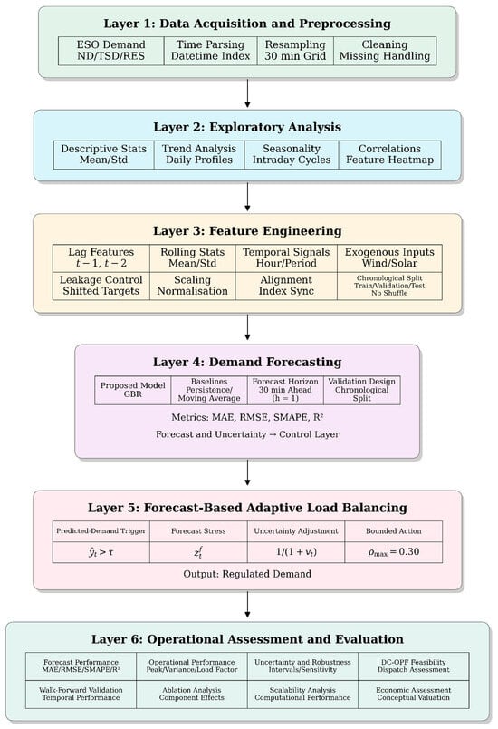
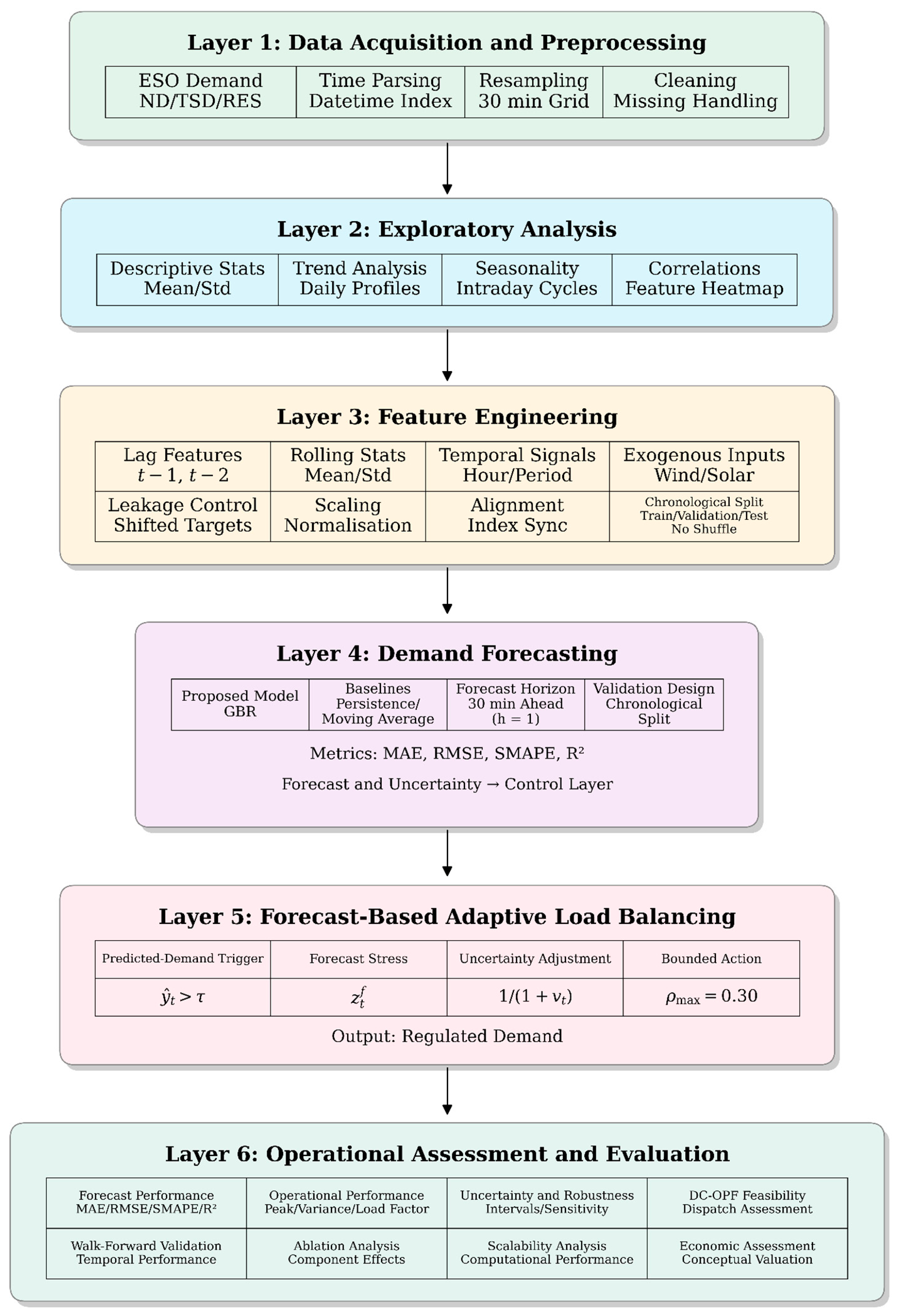
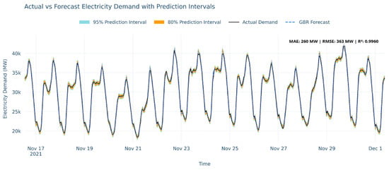
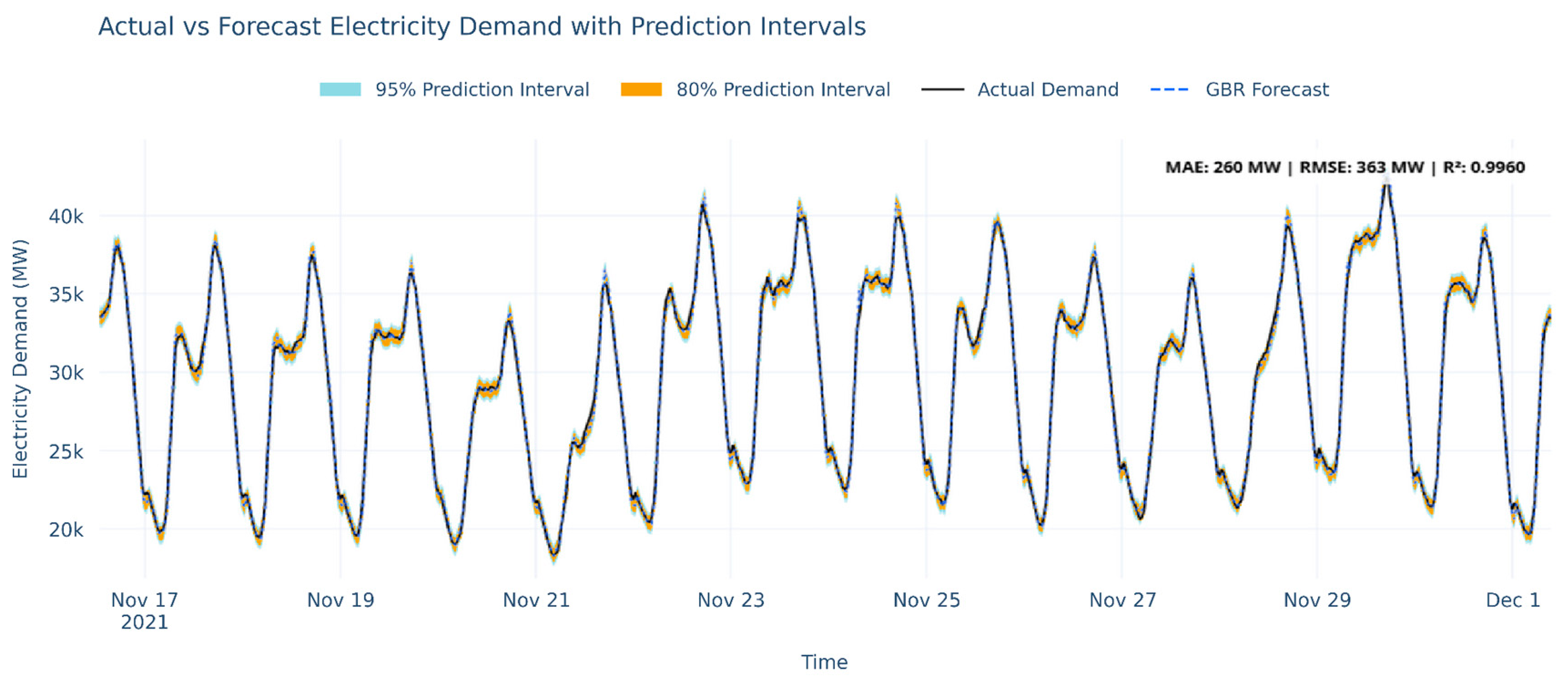
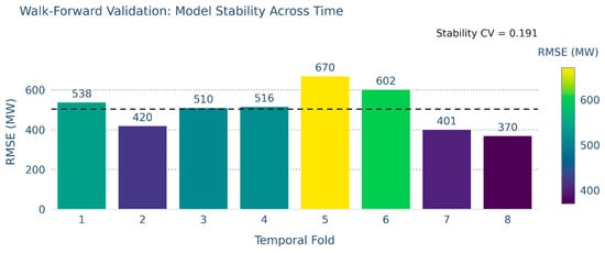
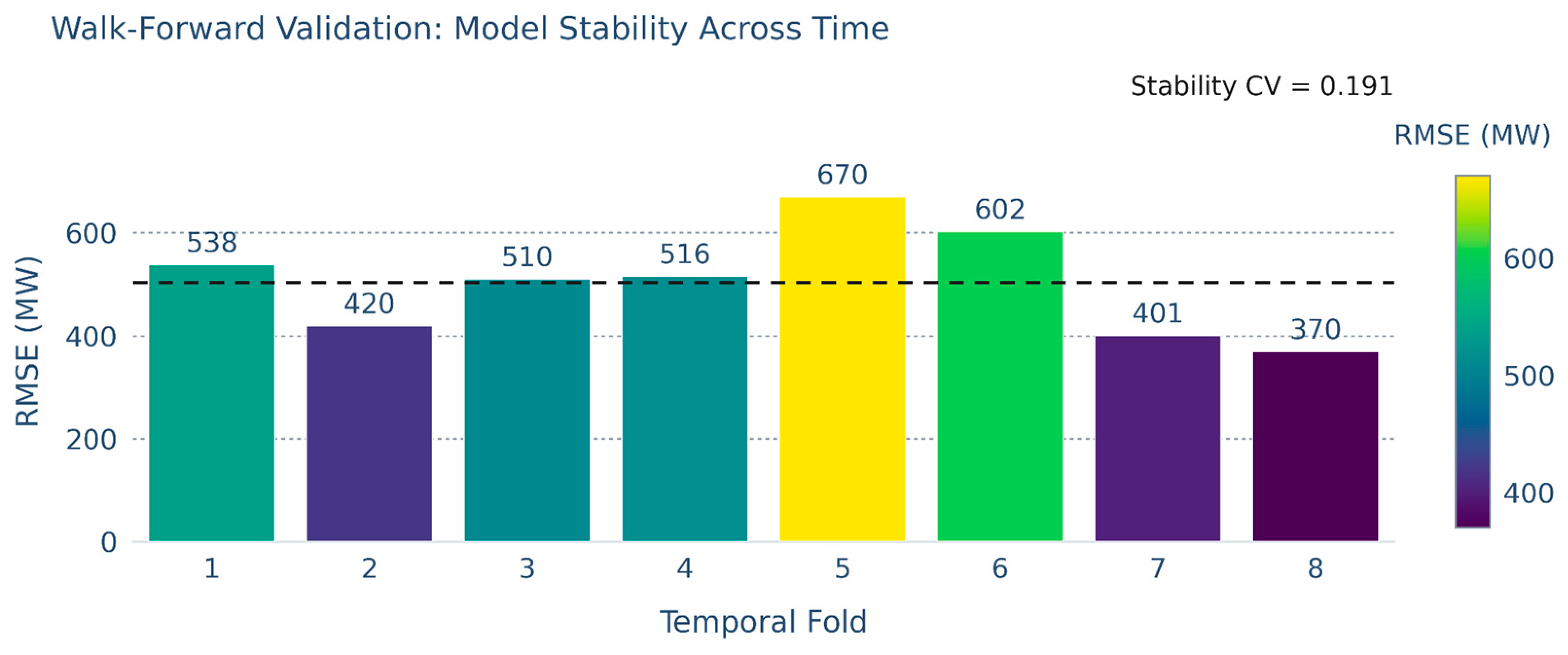
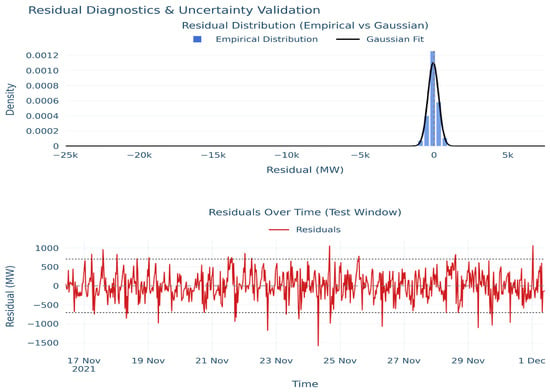
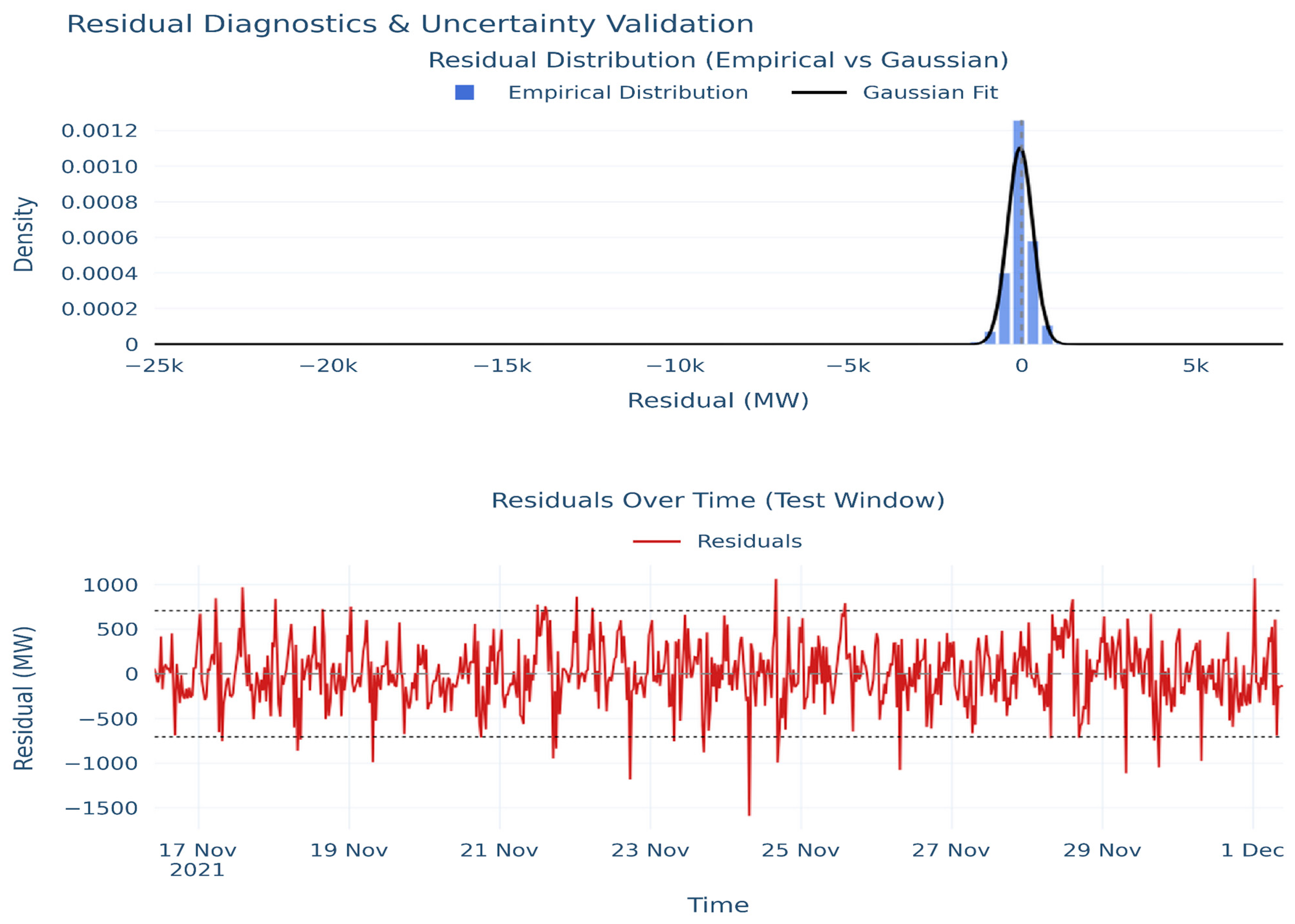
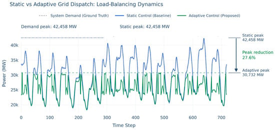
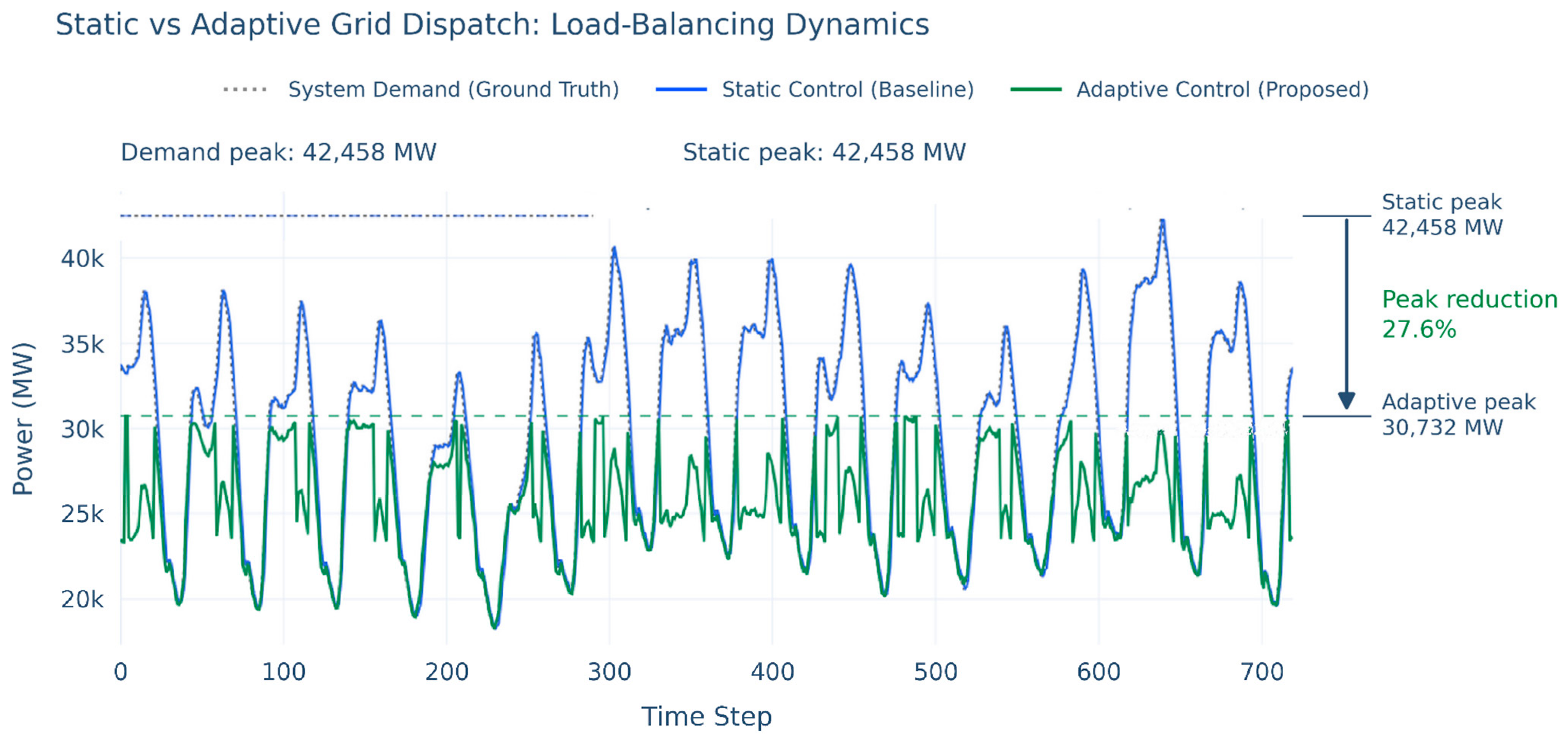
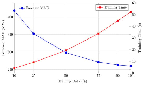
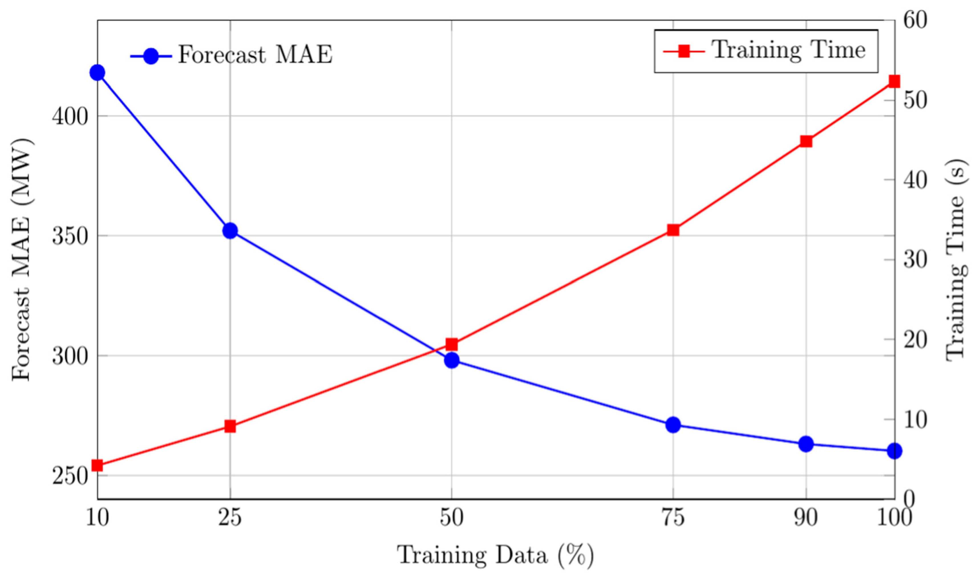
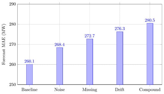
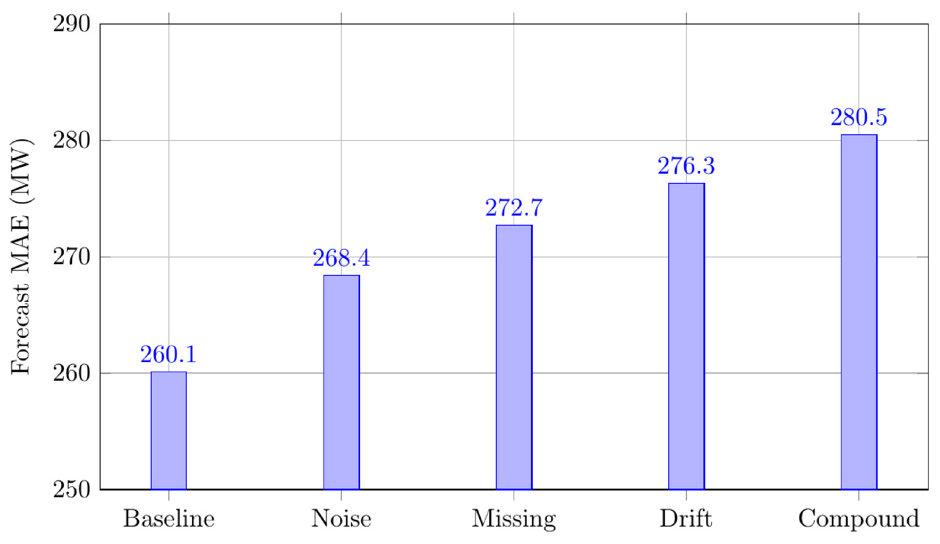
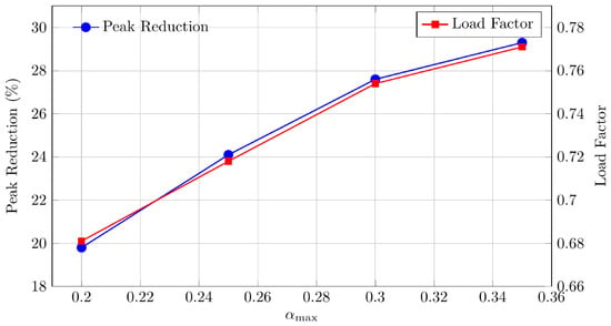
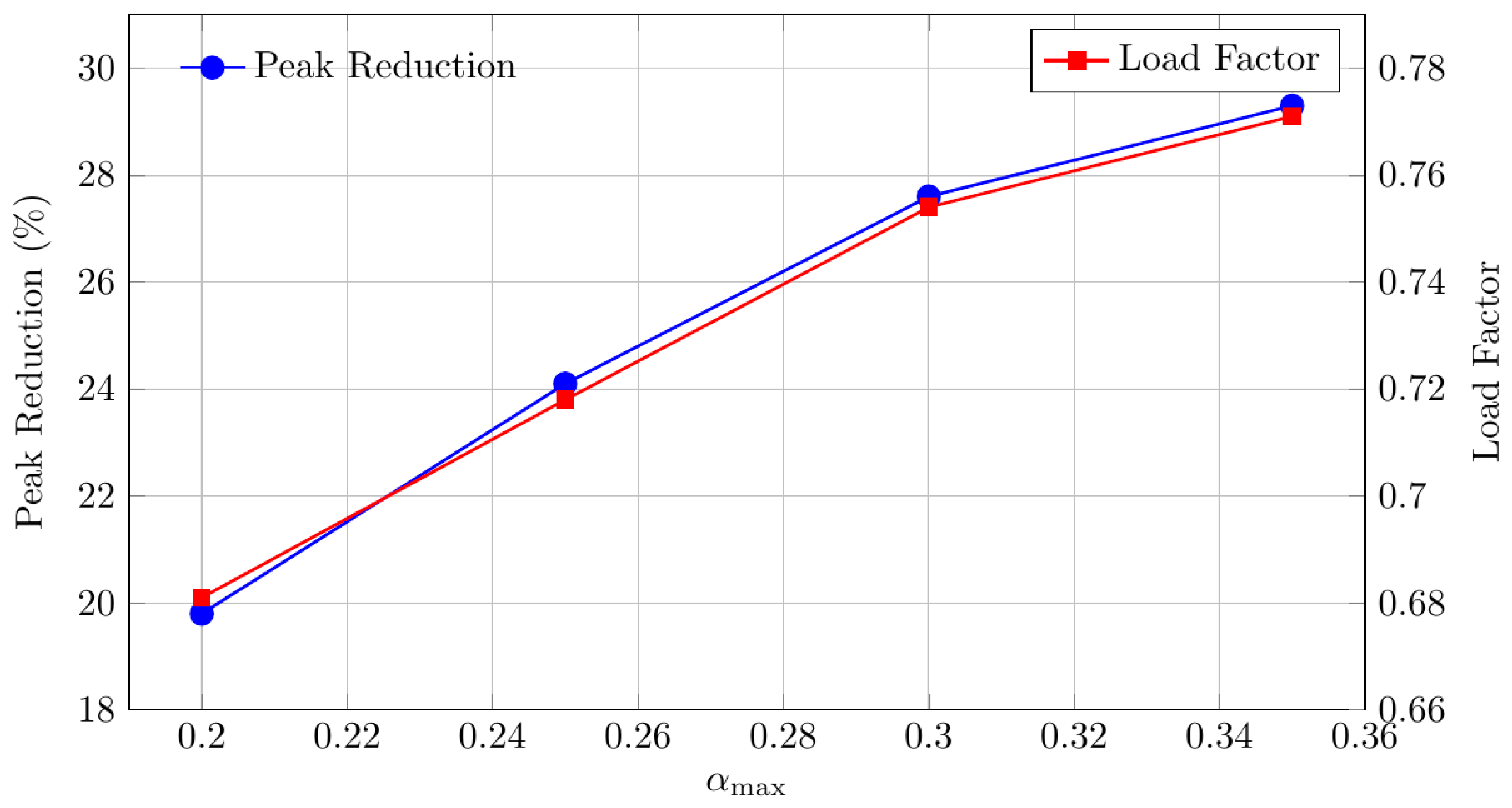

Disclaimer/Publisher’s Note: The statements, opinions and data contained in all publications are solely those of the individual author(s) and contributor(s) and not of MDPI and/or the editor(s). MDPI and/or the editor(s) disclaim responsibility for any injury to people or property resulting from any ideas, methods, instructions or products referred to in the content. |
© 2026 by the authors. Licensee MDPI, Basel, Switzerland. This article is an open access article distributed under the terms and conditions of the Creative Commons Attribution (CC BY) license.