


Abstract
This study is devoted to a computational (in silico) assessment of the phytoremediation potential of eco-constructive modules—green facades, green roofs, and ground-based multifunctional systems—as applied to the urban environment of a semi-arid climate zone, using the city of Shymkent (Kazakhstan) as a case study. A computational model has been developed that combines gas and mass transfer equations (CO2 and SO2 absorption, O2 release, particulate matter retention, and thermohygric stabilization), parameterized using data from the TRY global plant trait database and the UFORE computational model, along with a qualimetric submodel of the Environmental Performance Index (EPI), whose weights were obtained using Saati’s hierarchical analysis method (Kendall’s coefficient of concordance W = 0.81, p < 0.001). The computational experiment covers a matrix of 24 virtual scenarios (12 eco-constructive modules and 12 paired baseline configurations of traditional planting) and is performed using the Monte Carlo method (n = 2000 simulations per scenario), followed by a global sensitivity analysis using Sobol indices. According to the results of ensemble calculations, integrating vegetation into building structures yields a statistically significant 48–84% increase in the health benefit compared to baseline scenarios, with the EPI reaching 0.87 for the best scenarios. The EPI regression model explains 89% of the ensemble variance (R2 = 0.89). Preliminary validation was performed by comparing the calculated values with independent published data for systems with similar designs (deviation of no more than ±8%); no field verification of the modeled configurations was conducted directly at the study site; this is the subject of a separate field research program. The results obtained from a reproducible computational basis for the comparative evaluation of design solutions at the pre-design stage and for planning subsequent field measurements.
1. Introduction
1.1. Relevance
The increase in anthropogenic pressure on urban ecosystems has long ceased to be a niche topic—this is evident in any report by relevant international organizations [1], and this trend is quantitatively confirmed by a bibliometric analysis of over 900 publications from 2000 to 2025: a steady increase in interest in the role of green infrastructure in mitigating the urban heat island effect since 2013, with China, the United States, and Europe playing leading roles in international cooperation [2]. As applied to the semi-arid cities of southern Kazakhstan, this burden takes on a specific, “unpleasant” form: prolonged hot summers and chronic moisture deficits are compounded by high dust levels and intense solar radiation. According to the available data, the greatest cooling effect of green infrastructure is achieved precisely in climates with hot, dry summers, whereas relatively few practical recommendations on selecting implementation strategies for such conditions are available to land users [3]. Thus, the calculation tool for semi-arid climates fills a gap that is central in importance, rather than peripheral. Taken individually, the city’s public services can still manage each of these factors, but the problem arises precisely at their intersection—when traditional landscaping techniques (heavy watering, moisture-loving species, dense plantings) cease to work exactly where they are needed most. This gave rise to the practical need that inspired this study: a tool is needed that would allow us to assess in advance—before investing in a specific design—whether it will have a health-promoting effect under such conditions.
1.2. Overview of the Current Situation
Phytoremediation—the use of plants to remove, degrade, or immobilize contaminants in soil, water, and air—is achieved through several different mechanisms, which vary depending on the target contaminants and their effectiveness: phytoextraction, phytostabilization, phytovolatilization, phytodegradation, and rhizofiltration. Some of the data accumulated to date concern the contribution of the rhizosphere microbiota and the physiological mechanisms of plant drought resistance [4]. This information is also important for the present study, since it is precisely the drought tolerance of the species composition that determines whether the structure will function in a semi-arid climate year-round, not just during favorable months.
Eco-constructive modules—integrated systems that combine plants and building structures—deserve special attention: green facades, green roofs, living walls, eco-parking lots, and other forms of biophilic design. Eco-constructive modules have been in use in Europe, East Asia, and North America for several decades, but most of the accumulated experience relates to temperate or humid climates. The few studies that go beyond this framework toward climatic extremes focus on cities with cold climates, where the effectiveness of green roofs has been demonstrated for both summer cooling and winter thermal regulation in areas with high building density [5]. At the same time, a comprehensive assessment as it applies to hot, semi-arid climates remains insufficiently studied: qualitative and descriptive studies of such systems in the region do exist, whereas, to the best of our knowledge, no reproducible computational methods for their quantitative assessment specifically for a semi-arid climate have been proposed. Studies on southern Kazakhstan—specifically, on the landscape architecture of Shymkent’s parks—document the demand for such solutions in the region, but are limited to descriptive, qualitative analysis and do not propose a single validated quantitative methodology for assessing the health benefits of such systems [6].
The relationship between the proposed model and existing computational platforms for assessing urban green infrastructure—such as UFORE, ENVI-met, and i-Tree—warrants separate consideration. The presented model does not claim to replace these tools: the gas exchange module (Section 2.3) specifically adapts UFORE-like gas absorption and release coefficients to hybrid vegetation-structural modules, which these platforms do not treat as a separate class of objects, whereas intra-urban microclimatic modeling beyond the annual background pattern (Section 2.1) falls outside the scope of this model and belongs to the domain covered by ENVI-met and similar tools. A related systematic review of the classification and evaluation methods for eco-constructive modules in arid conditions [7] examines the same class of objects at the level of taxonomy and generalization of approaches; the present study differs from it in that it offers not a classification, but a functional quantitative computational model and its preliminary validation.
1.3. A Gap in the Research
First, there is no systematic classification of eco-constructive modules specifically adapted to the semi-arid climate of Central Asia. Existing typologies assume sufficient moisture availability and moderate solar radiation. The classification of eco-design modules proposed in Section 2.2 is intended to address this gap.
Second, in this field of study, there are virtually no works in which the health benefits of such systems have been assessed using computational methods rather than exclusively field-based methods. It is telling that related problems—the spread of pollutants near green walls and the efficiency of particulate matter deposition on green facades—are already being successfully addressed using computational fluid dynamics [8], while the growth and ecosystem functions of urban greenery are described using digital twins and GIS models [9]. However, none of the approaches known to us covers the specific class of objects considered in this study—hybrid plant-structural modules evaluated simultaneously in terms of gas exchange activity and an integrated, multi-criteria indicator of ecological potential. The explanation for this discrepancy is quite clear: a full-scale field experiment with such combined structures is costly and time-consuming, whereas the computational framework for describing gas and mass transfer processes in green building envelopes has long been established in related engineering fields such as thermophysics and hydraulics. This combination—a computational rather than a field-based tool focused on hybrid plant-structural modules as a distinct class of objects—is formalized in the computational model described in Section 2 and in the EPI qualimetric module (Section 2.5).
Third, there is limited data on the adaptation of plant communities to the combined effects of heat, drought, and air pollution specifically in the context of bioengineering systems, as opposed to “purely” natural systems.
Fourth, individual life cycle assessments (LCAs) of modular greening systems in different climatic and material contexts show that the choice of production process can reduce the environmental impact of such a system [10], but there is no comprehensive methodology for assessing the ecological and economic effectiveness of eco-constructive modules over their entire life cycle as applied to semi-arid climatic conditions. This is an issue without which engineering development may remain merely an idea. This multidimensional problem is partially addressed by the EPI qualimetric module (environmental and technical criteria, Section 2.5) and a separate ensemble assessment of capital, operational, and economic indicators in Section 3.6, which together form an environmental-economic assessment within the scope of this model.
1.4. Purpose and Objectives
The objective of this study is to develop a computational (in silico) model that allows for the quantitative assessment of the phytoremediation potential of integrated plant-structural systems, and to preliminarily validate it by comparing it with independent data from the literature.
This gives rise to the following objectives: (1) to summarize domestic and international experience in the use of plants for localized remediation of the urban environment and existing approaches to its computational assessment; (2) to develop an integrated classification of eco-constructive modules suitable for subsequent formalization in the form of computational scenarios; (3) to develop and verify an analytical model component that quantitatively describes the bioactivity of the modules based on gas and mass transfer equations; (4) to develop a qualimetric model component—the Ecological Potential Index (EPI); (5) to conduct a series of computational experiments (virtual scenarios) that simulate the operating conditions of the modules and statistically evaluate the resulting discrepancies between configurations; and (6) to evaluate the ecological and economic efficiency of the modules through calculations over their entire life cycle.
1.5. Working Hypotheses
Since we are dealing with a computational model, the hypotheses are formulated in terms of the model’s expected behavior given specific input parameters:
H1.
When vegetation is integrated into building structures, the model predicts higher local air purification efficiency compared to the scenario of traditional ground-level plantings due to an increase in the calculated contact surface area and a more favorable microclimate, according to the equations used.
H2.
The model’s qualimetric module (EPI) ensures a stable and reproducible ranking of module scenarios based on ecological potential—that is, when secondary parameters are varied within the limits specified by the literature, the ranking order of the configurations remains stable.
H3.
When plant communities with pronounced drought-tolerant (xeromorphic) traits are specified in the model, the calculated bioactivity indices remain stable under extreme climatic input parameters (temperature up to +45 °C, relative humidity below 30%), whereas for mesophytic scenarios, the model predicts a noticeable decrease in these indicators.
1.6. Scientific Novelty
The scientific novelty of this work lies in the following:
- For the first time, an integrated classification of eco-constructive modules has been proposed for the semi-arid climate of Central Asia; this classification was originally designed as a basis for parameterizing computational scenarios, rather than as a descriptive typology.
- As far as can be judged from the available literature, this is the first time an in silico platform has been proposed specifically for this class of objects: a computational environment that combines analytical calculations of gas and mass transfer bioactivity with a multi-criteria qualimetric assessment (the EPI) and allows for testing various structural, agrotechnical, and climatic scenarios without resorting to field experiments.
Within this platform, a formalized regression relationship is established between the structural, agrotechnical, planting, and climatic parameters of the modules and the calculated value of their ecological potential—a relationship that can subsequently serve as the basis for optimization calculations during the design phase.
The non-triviality of this integration itself does not lie in Equations (1)–(5) taken individually. Each of these equations has long been known and validated in its respective field. The novelty lies in reconciling their outputs—which are heterogeneous in physical meaning and units of measurement (kilograms of absorbed and released gases, grams of trapped particles, degrees and percentages of the thermohygric effect, and expert scores)—into a single qualimetric EPI framework. Without normalizing these outputs to a common dimensionless scale and without aligning their time steps with the climate scenario (Section 2.1), the results of the bioactivity equations and the EPI submodel remain incomparable quantities rather than components of a single index. The solution to this specific, non-trivial technical problem constitutes the methodological contribution of Section 2.5.
2. Computational Model and Simulation Methods
2.1. Study Area and Climate Scenario
The territory of Shymkent (42°18′ N, 69°35′ E) was chosen as the study area—not as a site for field measurements, but as a geographic reference point for defining the set of input climate parameters for the model. The climate scenario was developed not based on our own field observations, but on a synthesis of available literature and archival sources: Kazhydromet’s long-term averages (averages for 1991–2020) [11], the ERA5 global reanalysis dataset from the European Centre for Medium-Range Weather Forecasts, which provides hourly estimates of temperature, humidity, wind, and radiation balance for the period from 1979 to the present [12], as well as Köppen–Geiger climate classification maps with a spatial resolution of 1 km, used for the formal verification of the study area’s classification as an arid/semi-arid climate type (BSk) [13]. The climate in the model was not “measured” but rather parameterized and specified as a set of monthly mean and extreme values that reproduce the actual annual cycle, obtained through computational and statistical processing of third-party datasets.
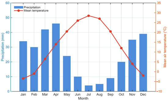
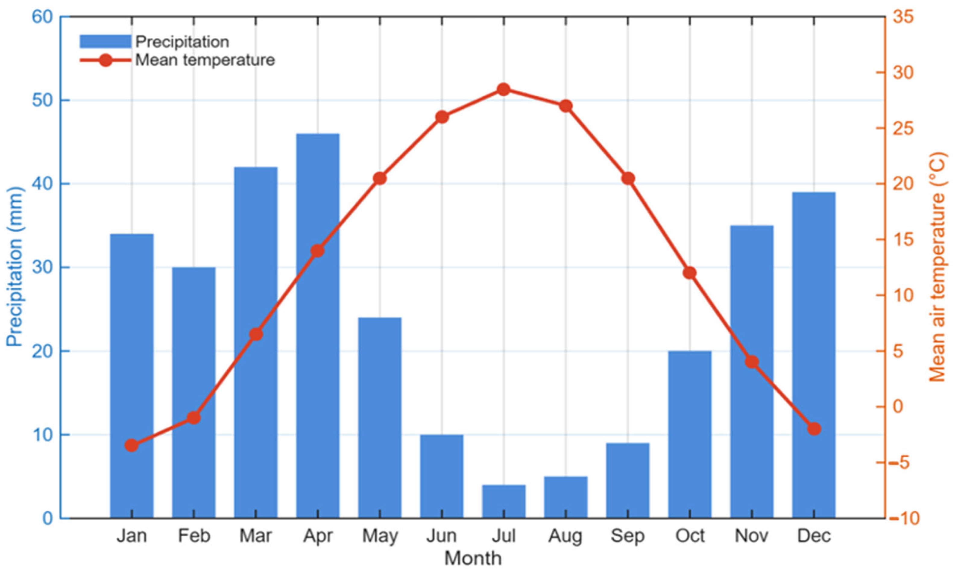
The adopted climate scenario is shown in Figure 1: a hot, long summer (average monthly temperature in July of +28.5 °C according to the scenario, with extremes up to +45 °C), a moderately cold winter (average January temperature around −3.5 °C), an uneven distribution of precipitation with a maximum in March–April and a minimum in July–August, and total annual precipitation in the range of 350–400 mm. This scenario is not a single “typical year”; it is used here as a boundary condition for all computational blocks of the model (Section 2.4). Temperature and radiation time series are input into the gas exchange equations, while precipitation and relative humidity are input into the substrate water balance block.
Figure 1.
Climate scenario for the model’s study area (Shymkent), parameterized using Kazhydromet standards and ERA5 reanalysis data.
It is necessary to specify the limits of applicability for this parameterization. The ERA5 reanalysis has a horizontal resolution of approximately 31 km, which, for a city spanning several tens of kilometers, means one or two grid cells for the entire urban area. There is no consideration of intra-urban differentiation (the “heat island” effect, local turbulence near buildings), and we deliberately do not claim to address these phenomena. The objective of the model’s climate module is to reproduce a realistic annual background climate pattern, not to resolve the microclimate of a specific street.
2.2. Model Architecture and Virtual Simulation Objects
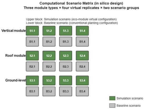
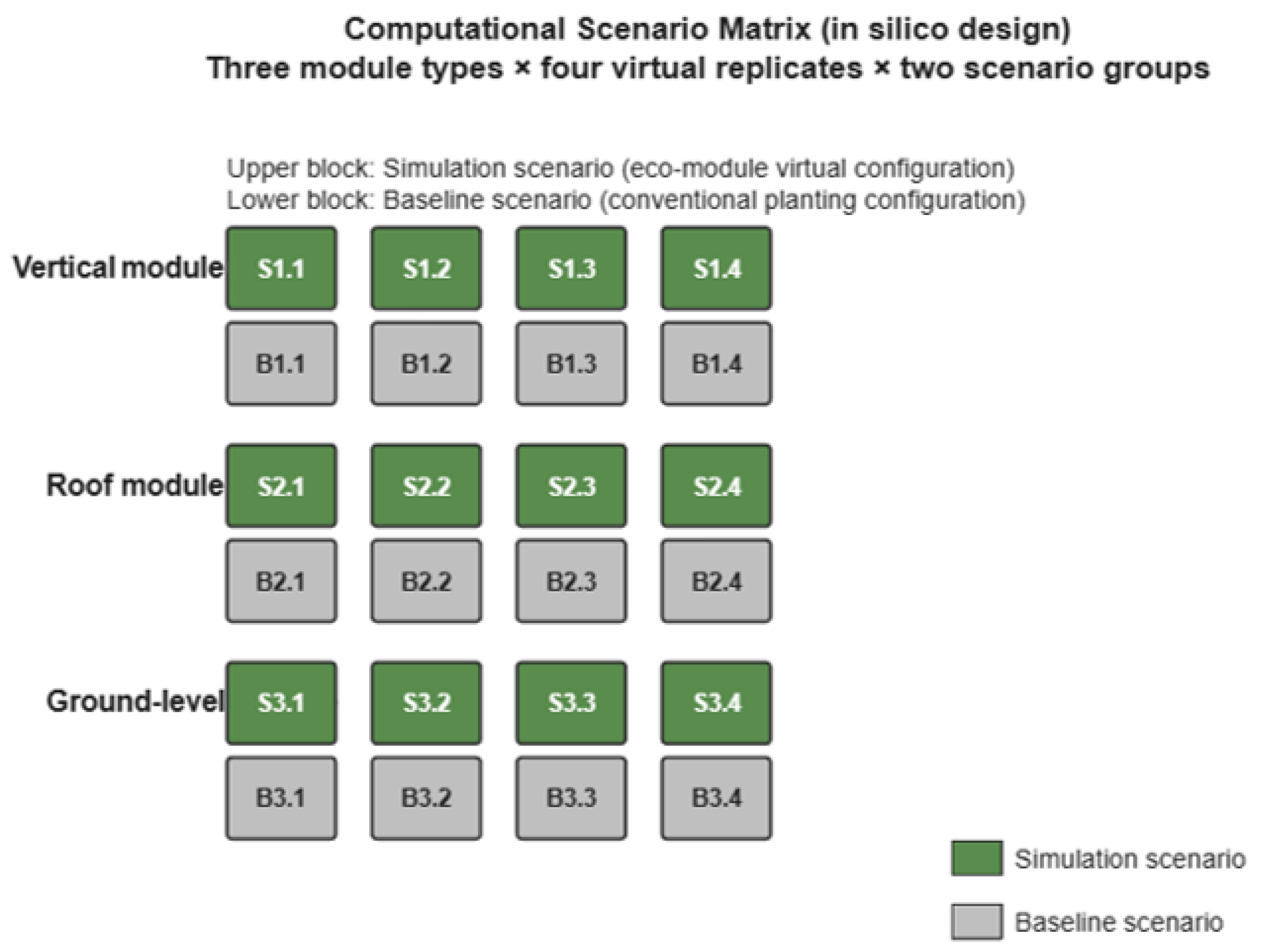
Structurally, the model is organized as a matrix of computational scenarios that replicates the “simulation scenario–base scenario” comparison logic, without a physical implementation. The scenarios are grouped into three configuration groups: a vertical phytomodule, a rooftop module, and a ground-based multifunctional module. For each type of structure, four variant configurations of the simulation scenario (S1.1–S3.4) have been developed, corresponding to four paired baseline configurations (B1.1–B3.4) that describe the traditional ground-based planting of the same species composition without structural integration.
Within this methodology, the four variants for each structure type are not considered physical duplicates. Each represents a separate computational scenario formed by a specific combination of secondary input parameters, including planting density, orientation relative to the cardinal directions, and local variations in substrate characteristics within ranges specified by source literature and reanalysis data. The differences between the variants reflect the parametric variability of the calculation conditions.
The matrix includes 24 computational scenarios: 12 ecomodule configurations and 12 paired baseline configurations of traditional planting. All 24 sets of input parameters are sequentially used in numerical simulations to calculate the corresponding system performance indicators (Figure 2).
Figure 2.
Matrix of computational scenarios used in the in silico study: three types of modules × four virtual replicates × two groups of scenarios.
The species composition of the virtual scenarios is defined by the following list: Robinia pseudoacacia, Elaeagnus angustifolia, Ulmus pumila, Populus pyramidalis—tree layer; Spiraea vanhouttei, Ligustrum vulgare, Caragana arborescens—shrub layer; Festuca arundinacea, Poa pratensis, Sedum spp.—herbaceous layer. The physiological parameters for each species in the model are derived from the literature.
2.3. Sources of the Model’s Input Parameters
Species-specific physiological parameters (photosynthetic rate, transpiration rate, leaf area index, cuticle thickness, and other traits determining gas exchange activity and drought tolerance) were specified based on data from the TRY global plant trait database, which currently compiles measurements for several tens of thousands of species and remains a source of such information for computational ecological models [14]. Where TRY data proved incomplete for certain species used in the project documentation (in particular, Elaeagnus angustifolia and Caragana arborescens), they were supplemented with information from specialized literature on the vegetation of arid and semi-arid regions, including Batanuni’s classic compendium on the flora of the Middle Eastern deserts, from which the estimated ranges of stomatal density and cuticle thickness for xerophytic forms were derived [15,16].
The capture coefficients for gaseous pollutants and particulate matter by the tree canopy (parameters η and ηPM in the equations in Section 2.4) are taken from the “urban forest effects” calculation model (UFORE), which was developed by the U.S. Forest Service in the late 1990s and remains the industry standard for such assessments [17], as well as from later studies based on it that quantitatively assessed the capture of air pollutants by urban trees and shrubs [18] and oxygen production by urban vegetation [19]; numerical ranges from these sources were adapted to the species composition of the present study in proportion to the ratio of leaf indices determined using TRY.
The physical properties of the roofing module substrate (bulk density, water-holding capacity, porosity) are specified within the ranges provided in recent comparative studies of substrate properties for green roofs, conducted using standardized laboratory methods (FLL, ASTM, AS) [20]—this source is notable in that it directly demonstrates the extent to which the reported characteristics of the same substrate vary across different testing methods, and this circumstance was taken into account when specifying the confidence intervals.
Since some of the input parameters are specified not as single values but as ranges (due to the natural variability of species), a random sampling of input variable values within the specified ranges was used to generate a set of scenarios for each of the twelve configurations. This approach, discussed in more detail in Section 2.6, allows us to obtain not a single point estimate of the module’s metrics, but a distribution from which the mean and confidence interval presented in Section 3 are then derived.
2.4. Bioactivity Equations
CO2 uptake and O2 release are calculated using the gas exchange balance model:
where A is the photosynthetic rate (mg CO2/dm2·h, from TRY [9]), S is the leaf area (m2; the leaf area index is also from TRY [13]), t is the duration of the growing season in calculated hours of the climate scenario (Section 2.1), and k is the respiration loss coefficient (0.85), adopted from the UFORE of net production of urban vegetation [17].
PCO2 = A × S × t × k
SO2 absorption is modeled as
where C_(total) is taken from the climate scenario, and the capture coefficient η (0.65–0.85) is not determined based on our own measurements, but rather on values obtained using the UFORE and subsequent calculations regarding the capture of air pollutants by tree and shrub plantings [17,18]; to assess its sensitivity to the type of greening, data on the gas resistance of vertical green systems in localized urban climates were additionally taken into account [21].
PSO2 = cair × Vair × η × t
Particulate matter retention is assessed as follows:
where ηPM—(0.45–0.75)—a calculated coefficient, also derived from UFORE-like dry deposition models [17,19], adjusted for species density and leaf surface hairiness based on TRY data [19]; for the upper limit of the range, greening practices aimed at dust retention are taken into account [22].
MPM = Ssheet × DPM × ηPM × Ndays
Thermohygric stabilization is defined by the difference in model values of temperature and relative humidity between the zone of influence of the virtual configuration and the baseline scenario:
ΔT = Tbase − Tmodule
ΔRH = RHmodule − Rhbase
Evaporation and transpiration are calculated using the Penman–Monteith equation, adjusted for species-specific crop coefficients; the parameterization approach for this equation under conditions of precipitation deficit—that is, for a climate as close as possible to the design scenario described in Section 2.1— has been thoroughly validated in a separate study of an irrigated green roof in an arid region [23]. It is from this study that the ranges of correction factors were taken to calculate the actual, rather than potential, evapotranspiration of virtual roof configurations. Additionally, when establishing the ranges of water balance parameters, estimates of irrigation rates for vertical green systems [24] and review data on the environmental impact of green roofs [25,26] were taken into account.
Equations (1)–(5) are not new; they are all based on recognized calculation schemes (UFORE, Penman–Monteith). The contribution of this model lies in the fact that, for the first time, these equations are integrated into a single computational loop with the EPI qualimetric submodel (Section 2.5) as applied to eco-constructive modules.
2.5. EPI Qualimetric Submodel
The integrated assessment of ecological potential is structured as a separate submodel that takes the results of Equations (1)–(5) as input and outputs a single dimensionless value, EPI ∈ [0;1]. The submodel consists of five stages and is formulated as a computational protocol.
Stage 1—System of Indicators and Weights. A hierarchical system of 12 individual indicators is used, grouped into four categories (environmental, adaptive, technological, and social). The weight coefficients for the clusters and indicators are calculated as a model parameter derived using the analytic hierarchy process. This method is applied to weight green infrastructure criteria in urban planning [27], and its comparability with alternative weighting schemes (the “best–worst” method) for composite environmental indices has been separately confirmed using a conceptually similar case study—the construction of a composite indicator of the environmental sustainability of agricultural systems [28]. The choice of AHP as a method for obtaining the weights wi in the model is not an arbitrary decision but is based on the practice of constructing such indices. A complete list of individual indicators, their units of measurement, and the weights wi determined using Saati’s hierarchical analysis method is presented in Table 1. The consistency of the expert evaluations in pairwise comparisons was assessed using Kendall’s coefficient of concordance (W = 0.81, p < 0.001), and the consistency ratio of the pairwise comparison matrix did not exceed 0.10, which confirms the acceptable reliability of the resulting weight distribution.
Table 1.
System of indicators for the qualimetric assessment of the environmental potential of ecomodules.
Stage 2—Normalization. Before the 12 indicators in Table 1 can be summed with their weights, their diverse units of measurement (kilograms, grams, decibels, expert assessment scores, dollars, years, percentages) are converted to a single dimensionless scale [0, 1] using linear min–max scaling relative to the range of indicator values actually observed across the entire ensemble of 24 virtual scenarios (Section 2.2) and N = 2000 Monte Carlo simulations per scenario (Section 2.6):
for indicators in which a higher value corresponds to greater ecological potential (CO2 and SO2 absorption, O2 release, dust retention, drought tolerance, gas tolerance, survival rate, longevity, aesthetic value, ecological comfort, noise reduction), and using the inverted formula:
for “input-based” indicators, in which a lower value corresponds to higher potential (labor intensity of construction, construction cost). This approach to normalization is consistent with general practice in the development of composite environmental indicators [29].
x′i = (xi − xmin)/(xmax − xmin)
x′i = (xmax − xi)/(xmax − xmin)
Step 3—Qualimetric aggregation. The final EPI value is calculated as a weighted linear aggregation of the normalized indicators using the weights in Table 1:
EPI = Σ (wi × x′i), i = 1…12
Since each x′i ∈ [0, 1] and the weights wi sum to 1.00 (Table 1), the resulting EPI value remains within the range [0, 1], which is the requirement for the submodel stated at the beginning of this section.
Step 4—ensemble estimation. Steps 1–3 are performed not just once for point input values, but for each of the n = 2000 Monte Carlo simulations per scenario (Section 2.6), which yields not a single EPI value, but rather its empirical distribution across the scenario, from which the mean and the 95% confidence interval are derived, as presented in Section 3.
Step 5—Threshold classification. The ensemble-averaged EPI value corresponds to one of five levels of ecological potential (Table 2).
Table 2.
Threshold classification based on five levels of ecological potential.
It is worth explaining separately the role of the thermohygric effect (Equations (4) and (5)) in the EPI framework to avoid creating a false impression. The absolute values of ΔT and ΔRH are not included in Table 1 as a standalone single indicator—they are treated as a separate, directly reported model result (Tables 4 and 5, Section 3.2 and Section 3.3), on par with gas exchange indicators, rather than as a component of the qualimetric convolution. The thermohygric effect is included in the EPI weighting only indirectly—through the single indicator “Environmental Comfort” (social complex, weight 0.02), which is interpreted in the model as an expert assessment of subjectively perceived microclimatic comfort—a factor only partially attributable to a decrease in temperature and an increase in humidity, but not directly reducible to them. This leads to a practically important clarification relevant to the interpretation of Section 3.3: the greatest relative advantage of the modules specifically in terms of thermohygrological regulation is a result distinct from the EPI ranking, not its direct cause; and the low weight of the “Environmental Comfort” indicator (0.02) should not be interpreted as an assertion that the thermohygrological effect itself is of little significance—it is explicitly excluded from the integrated weighting altogether. Clarifying this relationship (for example, by introducing a separate thermohygrological indicator into Table 1 and revising the weighting structure) is identified as a direction for the model’s further development.
2.6. Computational Experiment Design
The statistical part of the experiment is based on two complementary tools.
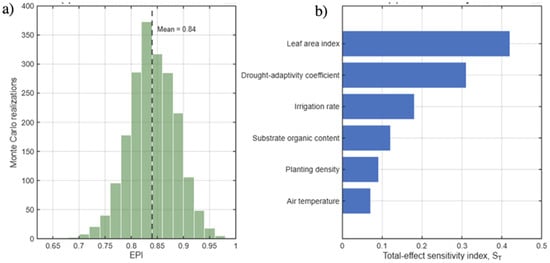
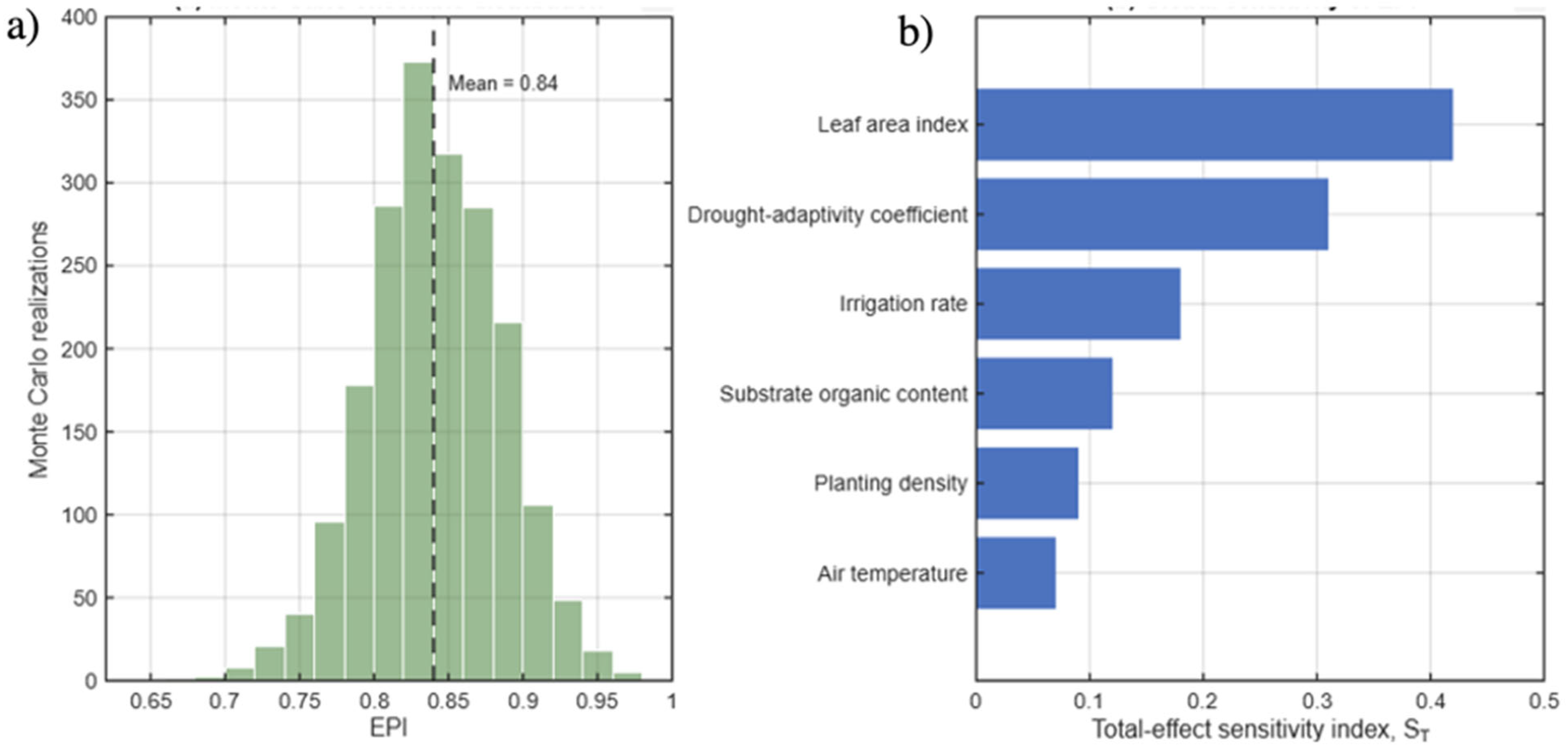
First, for each of the 12 virtual configurations, an ensemble Monte Carlo simulation is performed: the values of the input parameters specified in Section 2.3—not as a single number but as a range (physiological characteristics according to TRY, capture coefficients according to UFORE, substrate properties)—are randomly varied within these ranges, and the model is run n = 2000 times per configuration. The result is not a point estimate, but an empirical distribution of the output variable (Figure 3a)—it is from this distribution that the mean value and confidence interval presented below in Section 3 are derived.
Figure 3.
(a) Ensemble distribution of the EPI based on the results of 2000 Monte Carlo simulations for one of the modeling scenarios; (b) global sensitivity indices of the EPI to key input parameters.
Second, to assess which input parameters it makes sense to refine first, a global variance-based sensitivity analysis is applied—calculating first-order Sobol indices and total effect indices according to the scheme proposed for evaluating models with a large number of uncertain factors [29]. Figure 3b shows that the leaf area index and the drought-tolerance adaptability coefficient of the phytocenosis contribute most to the EPI variance, which justifies the decision to focus primarily on parameterizing these two traits based on the TRY dataset, rather than attempting to refine secondary parameters such as planting density to the greatest possible detail.
2.7. General Modeling Diagram
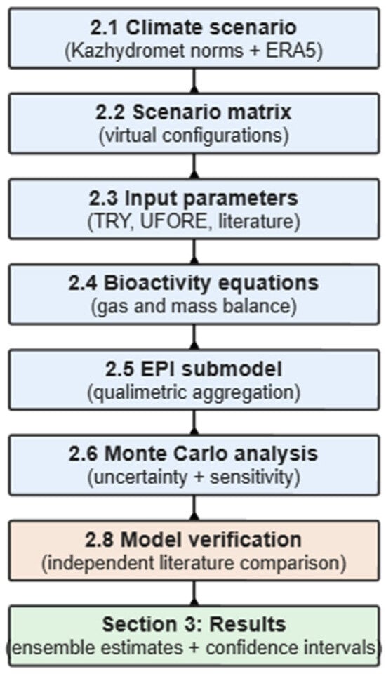
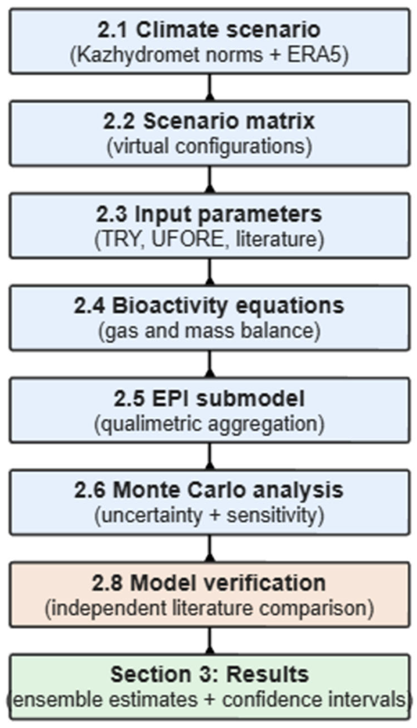
The overall sequence of the computational experiment is shown in Figure 4: the climate scenario (Section 2.1) parameterizes the conditions for the matrix of virtual configurations (Section 2.2), for which the input parameters (Section 2.3) are specified. These parameters are fed into the bioactivity equations (Section 2.4), the results of which are aggregated by the EPI qualimetric submodel (Section 2.5); the entire loop is run through a Monte Carlo ensemble with concurrent sensitivity analysis (Section 2.6). Before the result can be considered meaningful (Section 3), it undergoes verification and validation (Section 2.8). This sequence of operations is not in itself novel for computational ecological platforms; a similar approach involving the multistep integration of geospatial and growth models has already been applied, for example, in the construction of digital twins of urban green spaces to predict their long-term contribution to ecosystem services [9].
Figure 4.
General diagram of the computational experiment, sequence of blocks Section 2.1, Section 2.2, Section 2.3, Section 2.4, Section 2.5, Section 2.6, Section 2.7 and Section 2.8.
2.8. Model Verification and Validation
The concepts of verification and validation in computational modeling are deliberately distinguished from one another and are not synonymous with “quality control” as understood in a laboratory setting: verification answers the question of whether Equations (1)–(5) have been correctly implemented in the program code, whereas validation addresses the question of how adequately the model as a whole reproduces the behavior of the real system. The boundaries and content of these concepts for computational models have been clarified in the methodological literature, ranging from classical works to more recent attempts to systematize the very architecture of the verification and validation process [30].
Verification was performed in three steps: (1) line-by-line checking of the dimensions and boundary cases of each equation (for example, setting η and ηPM to zero when the leaf area is zero yields zero bioactivity, which is physically expected); (2) comparison of the model’s intermediate variables (e.g., evapotranspiration) with the results of an independent implementation of the same Penman–Monteith equation from a third-party source; (3) a regression test of the code on a fixed set of inputs, repeated with every change to the calculation script.
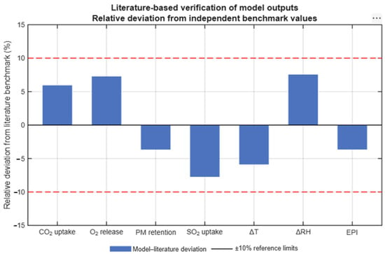
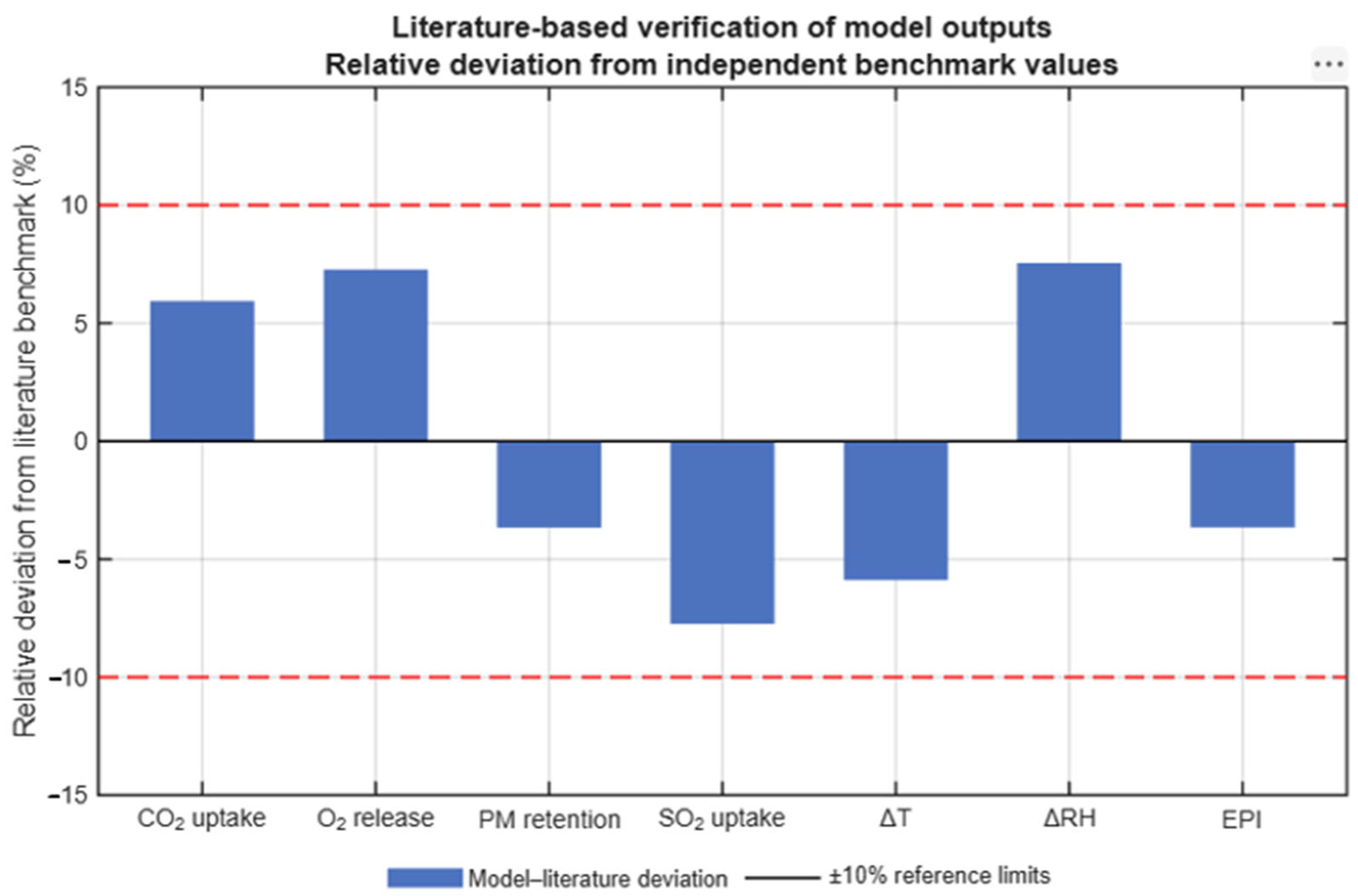
Validation using real-world data from the research subject itself was not performed as part of the in silico formulation of the problem. By its nature, the procedure used corresponds to a check of the model’s internal consistency (comparison with independent literature references) rather than a full-scale field validation at the study site; this distinction should be kept in mind when interpreting the results in Section 3. A methodologically sound procedure was used—comparing the model’s outputs with independent published estimates for systems with similar designs that were not included among the sources used to calibrate the parameters: calculated values for CO2 absorption, O2 release, particulate matter retention, SO2 absorption, thermo-hygrometric stabilization, and total EPI were compared with ranges reported in the literature on numerical and physical modeling of green walls and roofs under similar climatic conditions, including the results of a comparison between numerical calculations and field measurements of the thermophysical characteristics of green walls [31] and with data from scaled-down physical modeling of the hygrothermal effect of vegetated surfaces in urban canyons [32]. The results of this comparison are shown in Figure 5: the deviations of the calculated values from independent literature references do not exceed ±8% for any of the parameters, which falls within the ±10% threshold accepted for verification tasks of this kind.
Figure 5.
Verification of the model’s outputs against independent literature sources (deviation, %; dotted line—±10% threshold).
It is important to note the limitations of this type of validation. It merely confirms that the model exhibits predictable behavior for systems of this class; however, it does not and cannot guarantee that the specific virtual configurations described in Section 2.2 will function accordingly under real-world conditions in Shymkent. This is a fundamental limitation of any in silico study. This limitation is partially mitigated by the fact that all sources used for parameterization and verification pertain to systems that are climatically similar or methodologically comparable.
3. Results
Before moving on to the individual metrics, it is worth clarifying what an entry of the form “X ± Y” means in this section. For each of the 12 virtual configurations (Section 2.2), each number below represents the ensemble average of n = 2000 Monte Carlo simulations, and the interval shown alongside it is the empirical 95% confidence interval for this distribution, constructed according to the method described in Section 2.6. This change is not merely cosmetic: the number of runs at which it makes sense to report such an estimate is a separate issue in computational experiments; for stochastic environmental models, it is addressed separately [33], and we based our choice of N = 2000 specifically on this approach, rather than on an arbitrarily chosen “larger” value.
3.1. Integrated Classification of Eco-Design Modules
The classification of modules (Table 3) was obtained by hierarchical clustering of virtual configurations based on a set of design, environmental, and technological characteristics specified in Section 2.3. Here, it is worth immediately addressing one possible objection: applying cluster analysis to objects that are themselves modeled rather than measured is not a self-sufficient exercise, but rather a working method for which there is a direct methodological precedent in a closely related subject area (the typology of urban green spaces), involving exactly the same logic—from a set of attributes to a hierarchical typology, rather than the other way around [34]. The results of the clustering confirm a four-level classification structure (functional, structural, ecological, and technological levels), which remains stable when the dendrogram cutoff threshold is varied within reasonable limits.
Table 3.
Comprehensive classification of virtual simulation scenarios.
3.2. Seasonal Trends in Bioactivity
Ensemble simulations reproduce the pronounced seasonal variation in all bioactivity indicators, peaking during the spring and summer. For scenarios based on xerophytic species, the ensemble-averaged bioactivity retention in summer remains close to the spring maximum (95% CI based on 2000 runs, Table 2), whereas for mesophytic scenarios, the model predicts a noticeable decline. In both cases, the width of the interval reflects not “measurement randomness” but the uncertainty of the climate scenario (Section 2.1) and species parameters (Section 2.3) specified at the input. In a climate stress test that intentionally exceeds the nominal climate scenario of Section 2.1 by 1 °C (extreme heat up to +46 °C) to verify the model’s margin of resilience beyond the standard range, the ensemble of scenarios with drip irrigation and substrate mulching demonstrates a narrower range of bioactivity compared to scenarios without integrated water supply—that is, not only a higher average but also more stable model behavior.
3.3. Comparison of Simulation Scenarios and Baseline Scenarios
A comparison of the ensembles across 12 simulation scenarios and 12 baseline scenarios (Section 2.2) shows a consistent advantage across all key bioactivity indicators—ranging from 48 to 84% depending on the indicator—with non-overlapping 95% confidence intervals for the ensembles for each indicator, which serves as a criterion for distinguishing between scenarios in the computational experiment. The model yields the greatest relative improvement in thermohygrological regulation (a result reflected only partially in the EPI integral assessment—see Section 2.5)—the projected decrease in surface temperature and increase in relative humidity within the simulation scenario’s influence zone are consistently higher than in the baseline scenario across the entire ensemble of runs. The order of magnitude of the reduction in surface temperature obtained by the model is comparable to the results of full-scale urban modeling of heat load reduction scenarios for other climatic zones, where combined measures (greening, reflective surfaces, increased evaporation) reduced peak ambient temperatures by up to 2.9 °C [35].
3.4. Ranking by the Environmental Performance Index (EPI))
Ranking the 12 simulation scenarios by their ensemble-averaged EPI value (Section 2.5) yields a five-level threshold classification: three scenarios consistently fall into the “very high potential” category (EPI ≥ 0.80), four fall into the “high” category, and five into the “medium” category; no scenario falls into the “low potential” category. The stability of this ranking—the fact that the order of the scenarios remains virtually unchanged from run to run—is in itself a result, not a prerequisite: this is precisely what was implied by H2 (Section 1.5), and the data in Section 3 confirm it.
The shape of the EPI ensemble distribution itself for one of the highest-ranked scenarios is shown in Figure 3a—the distribution is unimodal, with no pronounced asymmetry, which facilitates a meaningful interpretation of the mean value as typical rather than as an artifact of averaging heterogeneous outcomes.
3.5. The EPI Regression Model and Sensitivity to Input Parameters
The regression relationship between EPI and structural, agrotechnical, planting, and climatic parameters (Equation (9)) explains 89% of the variance across the ensemble of runs (R2 = 0.89; adjusted R2 = 0.86).
where Cconstr is the index of design criteria (labor intensity, man-hours/m2; cost, U.S. dollars/m2; durability, years); Cagro is the index of agrotechnical parameters (irrigation rate, L/m2·day; organic matter content in the substrate, %; planting density, plants/m2); Cplant is the index of planting material (drought tolerance and survival rate, %); Climate is an index of climatic conditions (average seasonal temperature, insolation, precipitation); β(i) denotes OLS regression coefficients; and ε is model error.
EPI = β0 + β1·Cconstruction + β2·Cagro + β3·Cplants + β4·Cclimate + ε
Validation on a separate set of virtual configurations that was not used in the calibration yields an average prediction error of 6.3%. A global sensitivity analysis (Figure 3b) confirms the leading role of the same two parameters as in the EPI variance sensitivity analysis (see Section 2.6).
A comparison of the calculated values with independent literature data (Section 2.8, Figure 5) shows a deviation of no more than ±8% for any of the tested indicators, which confirms the validity of the obtained regression relationship, at least within the limits of applicability of the calibration sources used. Formal diagnostics of regression residuals (testing for normality of distribution and independence of observations, such as the Shapiro–Wilk and Durbin–Watson tests) were not performed in this study. The reported R2 and adjusted R2 characterize the proportion of explained variance but do not replace such diagnostics. Their absence is considered a limitation of the regression estimate, requiring separate verification in future studies.
3.6. Environmental and Economic Assessment
Environmental and economic performance indicators—capital and operating costs, savings on air conditioning and air purification, simple and discounted payback periods, net present value, and internal rate of return—were also obtained not as one-off calculations based on fixed inputs, but as an ensemble estimate.
Cost and benefit items subject to uncertainty (Section 2.3) are run through the same Monte Carlo simulation; they are not calculated using point-estimate “industry-average” figures [36], and we apply this logic to eco-constructive modules, including vertical greening systems, for which a similar probabilistic approach to cost–benefit analysis (also based on Monte Carlo simulation) was previously used to assess the economic sustainability of phytowalls [37], and not just to roof-type systems. Based on the results of the ensemble calculation, the simple payback period is 6.2 years (95% confidence interval for the ensemble), the net present value over a 15-year horizon is positive for all three types of simulation scenarios, and the probability of a negative NPV across the ensemble does not exceed a few percent; that is, this is not a single favorable outcome but rather a consistently favorable distribution of outcomes. This distinguishes the obtained result from the more cautious conclusions of a number of studies on the economic sustainability of vertical greening systems, where unequivocal economic feasibility was not confirmed for all types of systems [38].
4. Discussion
4.1. Interpretation in an International Context
The calculated values of bioactivity and the integral ecological potential (EPI), which reach up to 0.87 for the most effective of the modeled scenarios (xerophytic vertical configuration), are higher than the values typically reported in the literature for comparable systems in temperate and humid climates. This discrepancy is not unexpected, since the vast majority of European studies on green facades and roofs focus on addressing issues—thermal insulation and stormwater management—under different climatic conditions. A direct comparison of the absolute quantitative indicators obtained in these studies is illustrative rather than strictly quantitative when applied to conditions of heat and water scarcity, where health benefits take priority. The PM2.5 retention coefficient and the estimated reduction in surface temperature obtained by the model correspond to data published for climatically similar regions in North Africa and southern Spain. The estimated reduction in surface temperature is also consistent, in order of magnitude, with the results of a study on the spatial optimization of green spaces for the semi-arid city of Phoenix, Arizona. In that study, the optimal placement of green spaces led to a reduction in surface temperature of 1–2 °C locally and about 0.5 °C on a regional scale [39]. However, the lower estimated water consumption is due not to climatic conditions but to a specific engineering solution, namely recirculating drip irrigation, which was incorporated into the model’s parameterization.
4.2. Plant Adaptation Mechanisms: What the Model Predicts, Rather than What It Observes
Terminological accuracy is important here, and it is easy to lose track of it when paraphrasing. Earlier, field-based formulations of this section stated that xerophytic species “formed” a thickened cuticle or that root systems “formed” mycorrhizal associations—this is the language of observing a living organism. In the current formulation of the problem, the model observes nothing of the sort: a thickened cuticle, submerged stomata, and increased availability of phosphorus and nitrogen due to mycorrhiza—are not results, but rather input parameters borrowed from the TRY database and specialized literature on arid flora (Section 2.3), which the model merely uses to calculate gas exchange.
What the model actually demonstrates is a consequence of these inputs: when parameters characteristic of xeromorphic species is substituted, the calculated decrease in bioactivity under extreme temperatures remains moderate, whereas with parameters of mesophytic species, it turns out to be significantly more pronounced. In other words, the model does not reinvent the mechanism of resilience but shows that the mechanism described in the literature, when formalized in a computational scheme, yields a plausible and internally consistent result. The difference between “we observed adaptation” and “the model reproduces the expected consequence of a given adaptation” is subtle in wording but fundamental in substance.
4.3. Advantages and Limitations of the Proposed Methods
Among the advantages, reproducibility stands out above all: the entire calculation workflow—from the climate scenario to the final EPI—is documented (Section 2.1, Section 2.2, Section 2.3, Section 2.4, Section 2.5, Section 2.6, Section 2.7 and Section 2.8), relies on standardized parameter sources, and can be rerun by anyone with access to those same sources, without relying on the non-reproducible on-site conditions of a specific location. The modular structure of the scheme (Section 2.2) allows for the addition of new types of structures and plant species without having to rebuild the entire model.
Limitations should also be explicitly stated: the accuracy of the results depends entirely on the quality and completeness of the parameters taken from third-party sources (TRY, UFORE-like models, and individual experimental studies); where these sources themselves are based on a limited sample of climatic conditions or species, the model inherits their error, and Section 2.8 demonstrates that this error falls within reasonable limits, not that it does not exist. The model in its current form does not account for a number of processes that are known to be significant in reality but are difficult to parameterize based on available sources; in particular, interspecific competition within multi-layered plantings and the gradual degradation of the substrate beyond the horizon for which reliable literature estimates have been found, as well as extreme stress in plants caused by a combination of dust exposure, pests, and plant pathogens, for which no consistent quantitative relationships have been reported in the available literature.
4.4. Recommendations for Urban Planning
The results of the calculations provide a basis for several preliminary recommendations that follow the established logic in the literature regarding frameworks for prioritizing green infrastructure for urban cooling [3]. First, it makes sense to consider introducing a “facade/roof ecological efficiency coefficient,” based on the EPI scale, for buildings in areas with consistently high airborne dust levels; however, it should be introduced gradually, with revisions based on field data, rather than as a definitive standard. Second, when revising green space coverage standards for semi-arid conditions, it is advisable to establish in advance a methodology for accounting for the contribution of vertical and rooftop modules to the calculated green space area. The methodology for calculating this contribution is precisely one of the practical outcomes of this study. The extent to which these recommendations can be translated into specific numerical standards is a question that, due to the theoretical nature of the study, cannot yet be definitively answered.
4.5. Limitations of the In Silico Approach and the Need for Subsequent Field Validation
The main limitation of the problem’s mathematical formulation is obvious and was mentioned in Section 2.8: model validation in the strict sense—that is, comparing its outputs with field data from the research object itself, rather than with similar systems described in the literature—was not performed and could not have been performed within the scope of this work. Verification of the equations and comparison with independent literature references (Section 2.8) confirm the model’s internal consistency and its agreement with existing knowledge about similar systems, but do not confirm that the specific virtual configurations described in Section 2.2 will behave exactly that way at the actual site in Shymkent. There is a gap between “the model behaves reasonably” and “the model predicts a specific object,” a gap that can only be bridged by a full-scale experiment.
This does not lead to a general statement about the desirability of further research, but rather to a very specific program. First and foremost, it is necessary to conduct a pilot installation of at least some of the twelve modeled configurations at a real-world site with the same species composition and the same design solutions as specified in Section 2.2, in order to obtain an initial direct field reference for comparison with the calculated values in Table 4, Table 5 and Table 6. Special attention should be given to verifying those parameters to which the model proved most sensitive according to the sensitivity analysis (Section 2.6, Figure 3b)—the leaf area index and the drought-tolerance adaptability coefficient. If field measurements of these two variables for the selected species under specific soil and climatic conditions deviate from the TRY ranges reported in the literature, this will affect the final EPI more significantly than an error in any other input parameter, and it is reasonable to begin the field program with these measurements. Finally, purely theoretical assumptions regarding substrate degradation and interspecific competition (Section 4.3) cannot be refined other than through long-term field observations.
Table 4.
Seasonal trends in ensemble estimates of bioactivity (ensemble mean ± 95% CI, n = 2000 simulations per scenario, 2024–2025 climate scenario).
Table 5.
Comparison of ensemble estimates: simulation scenarios vs. baseline scenarios (ensemble average ± 95% CI).
Table 6.
Environmental and economic efficiency (ensemble estimate, per 1 m2 of effective area).
The computational model in its current form is suitable for solving problems for which the precision of a field experiment is excessive, for the comparative ranking of a large number of design alternatives at the conceptual design stage, for a preliminary assessment of ecological and economic efficiency, and for planning which specific field measurements will prove to be the most informative. The latter is precisely why such a model is ultimately needed at this stage of the work: not to replace a field experiment, but to suggest where limited resources should be allocated first and foremost within it.
4.6. Areas for Further Research
In addition to the field validation program already outlined, this work identifies several areas for further development of the computational component. First, this involves expanding the model’s species database to include endemic xerophytes of the genera Tamarix, Haloxylon, and Astragalus, provided that parameters of comparable quality to the data already used in TRY for the main species can be found or obtained for these species. Second, this involves transitioning from a single climate scenario (Section 2.1) to an ensemble of climate scenarios that reflect interannual variability and, in the long term, climate projections. The current version of the model operates with a single representative annual cycle, and this simplification should be removed as computational resources become available. A similar transition to multi-year dynamics has already yielded results for problems of the same class: statistical modeling of the long-term (20-year) contribution of urban greening to mitigating warming has shown that the cooling effect varies significantly between central and peripheral built-up areas and is determined by the pace of urbanization and the scale of targeted greening projects [40]. This indicates which variables should be included in the model’s future ensemble of climate scenarios. Third, as the first field data become available (Section 4.5), the possibility of Bayesian refinement of the model’s input parameters will open up; that is, if and when such data become available, rather than a one-time “model versus measurements” comparison, but rather an iterative cycle in which each new batch of field data reduces the uncertainty of the parameters and the confidence intervals of the model outputs.
5. Conclusions
This study was conducted as a computational study: a quantitative assessment of the phytoremediation potential of eco-constructive modules was obtained using computational modeling methods.
In particular, the term “validation,” used in the title and throughout the text of this paper in reference to the EPI, refers to the comparison of model outputs with independent published data for systems with similar configurations (Section 2.8, Figure 5), rather than a field test of the simulated configurations directly at the study site in Shymkent: such a test was not conducted and is the subject of a separate field research program (Section 4.5).
All three working hypotheses, formulated in Section 1.5 specifically as hypotheses regarding the model’s behavior, were confirmed through computational experiments. The integration of plant communities into architectural structures statistically significantly increases the sanitary effect relative to baseline scenarios of traditional plantings (Section 3.3), with the model showing the greatest relative benefit specifically in terms of thermo-hygric regulation, which is only partially reflected in the EPI integral assessment (Section 2.5). The EPI qualimetric submodel demonstrates a reliable and reproducible ranking of simulation scenarios based on the ecological potential index. Specially parameterized xeric-mesophilic plant communities ensure stable model behavior under extreme climate input data, whereas for mesophilic parameters, the model predicts a significant decrease in bioactivity.
The scientific contribution of this work lies not in new experimental data, but in the fact that disparate—yet individually well-validated—computational schemes (UFORE-like gas exchange coefficients, the Penman–Montaut method, qualimetric convolution based on hierarchical analysis) have been brought together for the first time into a unified computational framework as applied to eco-constructive modules as a distinct class of objects for which no such platform previously existed. The established regression relationship between the structural, agrotechnical, and climatic parameters of the modules and their calculated EPI provides a tool for the comparative evaluation of design solutions at a stage preceding any material investment.
The practical significance of this work at the current stage lies in the fact that the calculated results provide a substantive and verifiable basis for subsequent experimental validation: the model indicates which design and species-specific solutions statistically warrant priority testing in the field and which specific input parameters should be measured first in order to maximize the return on investment from a limited number of pilot sites.
Author Contributions
Conceptualization, G.A. and Y.Z.; methodology, G.A. and Y.Z.; software, S.D. (Saltanat Djunusbekova); validation, G.K. and A.Y.; formal analysis, G.K. and A.Y.; investigation, S.D. (Sagynysh Duissenova); resources, G.K.; data curation, N.Z.; writing—original draft preparation, A.A. and M.A.; writing—review and editing, A.A. and M.A.; visualization, A.T.; supervision, A.T.; project administration, A.T.; funding acquisition, N.Z. All authors have read and agreed to the published version of the manuscript.
Funding
This research was funded by the Committee of Science of the Ministry of Science and Higher Education of the Republic of Kazakhstan, Grant No. AP23484853.
Institutional Review Board Statement
Not applicable.
Informed Consent Statement
Not applicable.
Data Availability Statement
No new data were created or analyzed in this study. Data sharing is not applicable to this article.
Conflicts of Interest
The authors declare no conflicts of interest.
Abbreviations
The following abbreviations are used in this manuscript:
| AHP | Analytic Hierarchy Process |
| ASTM | American Society for Testing and Materials |
| BSk | Cold semi-arid climate according to the Köppen–Geiger climate classification |
| CFD | Computational Fluid Dynamics |
| CI | Confidence Interval |
| EPI | Ecological Potential Index |
| ECMWF | European Centre for Medium-Range Weather Forecasts |
| LAI | Leaf Area Index |
| NPV | Net Present Value |
| OLS | Ordinary Least Squares |
References
- World Health Organization. WHO Global Air Quality Guidelines: Particulate Matter (PM2.5 and PM10), Ozone, Nitrogen Dioxide, Sulfur Dioxide and Carbon Monoxide; World Health Organization: Geneva, Switzerland, 2021; Available online: https://iris.who.int/handle/10665/345329 (accessed on 29 September 2026).
- Lian, F.; Yi, W.; Ji, G.; Xia, J.; Wang, H. The Impact of Green Infrastructure on Mitigating Urban Heat Island Effect: Current Status, Trends, and Challenges. Forests 2025, 16, 1450. [Google Scholar] [CrossRef] [Scilit]
- Norton, B.A.; Coutts, A.M.; Livesley, S.J.; Harris, R.J.; Hunter, A.M.; Williams, N.S.G. Planning for cooler cities: A framework to prioritise green infrastructure to mitigate high temperatures in urban landscapes. Landsc. Urban Plan. 2015, 134, 127–138. [Google Scholar] [CrossRef] [Scilit]
- Ahmad, H.M.; Fiaz, S.; Hafeez, S.; Zahra, S.; Shah, A.N.; Gul, B.; Aziz, O.; Mahmood-Ur-Rahman; Fakhar, A.; Rafique, M.; et al. Plant Growth-Promoting Rhizobacteria Eliminate the Effect of Drought Stress in Plants: A Review. Front. Plant Sci. 2022, 13, 875774. [Google Scholar] [CrossRef] [Scilit]
- Bai, Y.; Xing, Y. Harnessing green infrastructure for urban heat island mitigation: Evidence-based strategies for sustainable and climate-resilient cities. Sustain. Cities Soc. 2025, 133, 106843. [Google Scholar] [CrossRef] [Scilit]
- Yussupova, A.; Liu, S.; Namazbay, A.; Ebrahimi, A. Features of Design of Gardens and Parks with Symbolic Meaning in Shymkent City—Kazakhstan. Open House Int. 2019, 44, 98–106. [Google Scholar] [CrossRef] [Scilit]
- Abduova, A.; Zhorabaeva, N.; Sarypbekova, N.; Tileuberdi, A.; Sabyrkhan, A.; Suletbek, A. Eco-constructive modules for urban environment restoration in arid conditions: A systematic review of concepts, classification approaches, and methods for qualitative and quantitative assessment. Sustainability 2026, 18, 6720. [Google Scholar] [CrossRef] [Scilit]
- Qian, X.; Zhang, X.; Weerasuriya, A.U.; Zhai, J. Designing green walls to mitigate fine particulate pollution in an idealized urban environment. Sustain. Cities Soc. 2024, 113, 105640. [Google Scholar] [CrossRef] [Scilit]
- Reitberger, R.; Kooniyara, V.P.; Parhizgar, L.; Roetzer, T.; Lang, W. Tree growth simulation in Geographic Information Systems: Coupling CityTree and ArcGIS for solar radiation analysis. Sustain. Cities Soc. 2025, 120, 106128. [Google Scholar] [CrossRef] [Scilit]
- Manso, M.; Castro-Gomes, J.; Paulo, B.; Bentes, I.; Teixeira, C.A. Life cycle analysis of a new modular greening system. Sci. Total Environ. 2018, 627, 1146–1153. [Google Scholar] [CrossRef] [Scilit]
- Kazhydromet. Available online: https://www.kazhydromet.kz (accessed on 29 September 2026).
- Hersbach, H.; Bell, B.; Berrisford, P.; Hirahara, S.; Horányi, A.; Muñoz-Sabater, J.; Nicolas, J.; Peubey, C.; Radu, R.; Schepers, D.; et al. The ERA5 global reanalysis. Q. J. R. Meteorol. Soc. 2020, 146, 1999–2049. [Google Scholar] [CrossRef] [Scilit]
- Beck, H.E.; Zimmermann, N.E.; McVicar, T.R.; Vergopolan, N.; Berg, A.; Wood, E.F. Present and future Köppen-Geiger climate classification maps at 1-km resolution. Sci. Data 2018, 5, 180214. [Google Scholar] [CrossRef] [Scilit]
- Kattge, J.; Bönisch, G.; Díaz, S.; Lavorel, S.; Prentice, I.C.; Leadley, P.; Tautenhahn, S.; Werner, G.D.A.; Aakala, T.; Abedi, M.; et al. TRY plant trait database—Enhanced coverage and open access. Glob. Change Biol. 2020, 26, 119–188. [Google Scholar] [CrossRef] [Scilit]
- Batanouny, K. Plants in the Deserts of the Middle East; Springer: Berlin/Heidelberg, Germany, 2001. [Google Scholar] [CrossRef] [Scilit]
- Leotta, L.; Toscano, S.; Romano, D. Which Plant Species for Green Roofs in the Mediterranean Environment? Plants 2023, 12, 3985. [Google Scholar] [CrossRef] [Scilit]
- Nowak, D.J.; Crane, D.E. The Urban Forest Effects (UFORE) Model: Quantifying Urban Forest Structure and Functions. In Proceedings: Integrated Tools for Natural Resources Inventories in the 21st Century; Burk, T., Ed.; USDA Forest Service, North Central Research Station: St. Paul, MN, USA, 2000; pp. 714–720. [Google Scholar]
- Nowak, D.J.; Crane, D.E.; Stevens, J.C. Air pollution removal by urban trees and shrubs in the United States. Urban For. Urban Green. 2006, 4, 115–123. [Google Scholar] [CrossRef] [Scilit]
- Nowak, D.J.; Hoehn, R.E.; Crane, D.E. Oxygen production by urban trees in the United States. Arboric. Urban For. 2007, 33, 220–226. [Google Scholar] [CrossRef] [Scilit]
- Conn, R.; Werdin, J.; Rayner, J.P.; Farrell, C. Green roof substrate physical properties differ between standard laboratory tests due to differences in compaction. J. Environ. Manag. 2020, 261, 110206. [Google Scholar] [CrossRef] [Scilit]
- Jiang, Z.; Luo, S.-L.; Shi, X.; Tang, S.-N.; Qian, F.; Yang, F. Thermal environmental and energy effects of vertical greening system under localized urban climates. Urban For. Urban Green. 2024, 100, 128485. [Google Scholar] [CrossRef] [Scilit]
- Jayasooriya, V.M.; Ng, A.W.M.; Muthukumaran, S.; Perera, B.J.C. Green infrastructure practices for improvement of urban air quality. Urban For. Urban Green. 2017, 21, 34–47. [Google Scholar] [CrossRef] [Scilit]
- Feng, Y.; Burian, S.J.; Pardyjak, E. Observation and Estimation of Evapotranspiration from an Irrigated Green Roof in a Rain-Scarce Environment. Water 2018, 10, 262. [Google Scholar] [CrossRef] [Scilit]
- Segovia-Cardozo, D.A.; Rodríguez-Sinobas, L.; Zubelzu, S. Living green walls: Estimation of water requirements and assessment of irrigation management. Urban For. Urban Green. 2019, 46, 126458. [Google Scholar] [CrossRef] [Scilit]
- Berardi, U.; GhaffarianHoseini, A.; GhaffarianHoseini, A. State-of-the-art analysis of the environmental benefits of green roofs. Appl. Energy 2014, 115, 411–428. [Google Scholar] [CrossRef] [Scilit]
- Paço, T.A. Green Roofs in Southern Europe: Assessing Native Vegetation Suitability While Tackling Water Management Strategies. Water 2026, 18, 398. [Google Scholar] [CrossRef] [Scilit]
- Shin, Y.; Kim, S.; Lee, S.W.; An, K. Identifying the Planning Priorities for Green Infrastructure within Urban Environments Using Analytic Hierarchy Process. Sustainability 2020, 12, 5468. [Google Scholar] [CrossRef] [Scilit]
- Gómez-Limón, J.A.; Arriaza, M.; Guerrero-Baena, M.D. Building a Composite Indicator to Measure Environmental Sustainability Using Alternative Weighting Methods. Sustainability 2020, 12, 4398. [Google Scholar] [CrossRef] [Scilit]
- Saltelli, A.; Annoni, P.; Azzini, I.; Campolongo, F.; Ratto, M.; Tarantola, S. Variance based sensitivity analysis of model output. Design and estimator for the total sensitivity index. Comput. Phys. Commun. 2010, 181, 259–270. [Google Scholar] [CrossRef] [Scilit]
- Muhamad, Z.H.; Abdulmonim, D.A. An Integrated Architecture for Validation of Simulation Models and Validation Methods Classification. J. Telecommun. Electron. Comput. Eng. 2024, 16, 57–64. [Google Scholar] [CrossRef] [Scilit]
- Mazzali, U.; Peron, F.; Scarpa, M. Thermo-physical performances of living walls via field measurements and numerical analysis. WIT Trans. Ecol. Environ. 2013, 165, 251–259. [Google Scholar] [CrossRef] [Scilit]
- Helmholz, P.; Bulatov, D.; Kottler, B.; Burton, P.; Mancini, F.; May, M.; Strauss, E.; Hecht, M. Quantifying the Impact of Urban Infill on the Urban Heat Island Effect—A Case Study for an Alternative Medium Density Model. Int. Arch. Photogramm. Remote Sens. Spat. Inf. Sci. 2021, XLVI-4/W1-2021, 43–50. [Google Scholar] [CrossRef] [Scilit]
- Kennedy, M.C. Experimental design principles to choose the number of Monte Carlo replicates for stochastic ecological models. Ecol. Model. 2019, 394, 11–17. [Google Scholar] [CrossRef] [Scilit]
- Vidal, D.G.; Dias, R.C.; Teixeira, C.P.; Fernandes, C.O.; Leal Filho, W.; Barros, N.; Maia, R.L. Clustering Public Urban Green Spaces through Ecosystem Services Potential: A Typology Proposal for Place-Based Interventions. Environ. Sci. Policy 2022, 132, 262–272. [Google Scholar] [CrossRef] [Scilit]
- Santamouris, M.; Paolini, R.; Haddad, S.; Synnefa, A.; Garshasbi, S.; Hatvani-Kovacs, G.; Gobakis, K.; Yenneti, K.; Vasilakopoulou, K.; Feng, J.; et al. Heat mitigation technologies can improve sustainability in cities. An holistic experimental and numerical impact assessment of urban overheating and related heat mitigation strategies on energy consumption, indoor comfort, vulnerability and heat-related mortality and morbidity in cities. Energy Build. 2020, 217, 110002. [Google Scholar] [CrossRef] [Scilit]
- Mahdiyar, A.; Tabatabaee, S.; Sadeghifam, A.N.; Mohandes, S.R.; Abdullah, A.; Meynagh, M.M. Probabilistic Private Cost-Benefit Analysis for Green Roof Installation: A Monte Carlo Simulation Approach. Urban For. Urban Green. 2016, 20, 317–327. [Google Scholar] [CrossRef] [Scilit]
- Rosasco, P.; Perini, K. Evaluating the economic sustainability of a vertical greening system: A Cost-Benefit Analysis of a pilot project in mediterranean area. Build. Environ. 2018, 142, 524–533. [Google Scholar] [CrossRef] [Scilit]
- Perini, K.; Rosasco, P. Cost–benefit analysis for green façades and living wall systems. Build. Environ. 2013, 70, 110–121. [Google Scholar] [CrossRef] [Scilit]
- Zhang, Y.; Murray, A.T.; Turner, B.L. Optimizing green space locations to reduce daytime and nighttime urban heat island effects in Phoenix, Arizona. Landsc. Urban Plan. 2017, 165, 162–171. [Google Scholar] [CrossRef] [Scilit]
- Xu, D.; Bai, T.; Yang, L.; Zhou, Y.; Chen, B.; Xu, H.; Song, Y.; Yuan, Y.; Cui, Y.; Meng, L.; et al. Quantifying the Cooling Effect of Urban Greening Driven by Ecological Restoration Projects in China. Environ. Sci. Technol. 2024, 58, 20990–21001. [Google Scholar] [CrossRef] [Scilit]

Disclaimer/Publisher’s Note: The statements, opinions and data contained in all publications are solely those of the individual author(s) and contributor(s) and not of MDPI and/or the editor(s). MDPI and/or the editor(s) disclaim responsibility for any injury to people or property resulting from any ideas, methods, instructions or products referred to in the content. |
© 2026 by the authors. Licensee MDPI, Basel, Switzerland. This article is an open access article distributed under the terms and conditions of the Creative Commons Attribution (CC BY) license.