Decomposing Climate Policy Uncertainty and Systemic Banking Risk in the United States: Implications for Sustainable Finance

Abstract

Climate policy uncertainty is usually measured as a single index, which cannot tell supervisors whether risk to banks comes from Congress, federal agencies, or international commitments. This study separates these channels. Because banks provide much of the credit needed for the low-carbon transition, knowing where this risk comes from matters for sustainable finance as well as for financial stability. We build legislative and regulatory indices that count formal attempts to block, delay, or reverse existing U.S. climate policy, alongside an international-commitment index and a market-based transition uncertainty measure. Using monthly data from January 2005 to December 2024, a quantile VAR with frequency decomposition, a time-varying model, and bias-corrected bootstrap inference, we trace spillovers to G-SIB, regional and broker-dealer equity risk, G-SIB CDS spreads, and ΔCoVaR. In normal months, climate policy uncertainty has little measurable effect on bank risk once broader financial conditions are controlled for. Spillovers emerge in the tails and build within a quarter. Regulatory reversal risk outweighs the international and market channels when bank risk rises fastest, but no more than contested legislation does. In the tails, the resolution of policy fights moves bank risk more than their outbreak, and legislative spillovers disappear when contested bills are replaced by the volume of climate legislation. Climate stress scenarios should therefore center on contestation episodes and tail states. Because a stable banking system is needed to fund the transition, the findings show that predictable and durable climate policy supports both financial stability and sustainable development.

1. Introduction

In less than a decade, the U.S. banking system has lived through three distinct climate policy regimes: the regulatory push that culminated in the Clean Power Plan in 2015, the rollback and Paris withdrawal of 2017–2020, and the re-engagement anchored by the Inflation Reduction Act in August 2022. Each shift was fought over in Congress, in the Federal Register, and in international negotiations. Whether these fights reached bank balance sheets, and through which channel, is still an open question. Most of the finance literature treats climate policy uncertainty (CPU) as a single index [1,2], which mixes forces with different institutional origins, different speeds, and different degrees of reversibility.

These questions also matter for sustainability. Meeting the goals of the Paris Agreement and the UN Sustainable Development Goals, in particular SDG 7 (affordable and clean energy), SDG 8 (decent work and economic growth) and SDG 13 (climate action), requires large and long-lived investment in clean energy, efficient buildings and low-carbon infrastructure, and banks are a key source of finance for this investment [3]. When the path of climate policy is unclear, banks find it harder to price transition risk, may hold back long-term lending to green projects, and may face sudden losses on carbon-intensive loans if policy changes direction. Climate policy uncertainty can therefore weaken both financial stability and the flow of credit that the low-carbon transition needs. Knowing which sources of policy uncertainty reach banks, and when, is thus a question for sustainable finance as well as for banking supervision: a banking system that stays stable through policy shifts is better placed to support a steady and orderly transition.

The distinction has economic content. Legislative uncertainty moves with congressional bargaining and the electoral cycle. Regulatory uncertainty arises when agency rules are delayed, stayed, reconsidered, or repealed, which can happen without any new legislation. International-commitment uncertainty follows treaty accession and withdrawal and bears most directly on cross-border and sovereign exposures. In our data, the legislative and international sub-indices are essentially uncorrelated (Section 3.3), so an aggregate index may obscure the channels through which climate policy affects banks. Markets also price transition uncertainty directly. The gap between the realized volatility of clean-energy and fossil-energy equities offers a market-based counterpart to the narrative measures.

Measurement matters as much as aggregation. A rising count of climate bills or rules can mean that government is doing more, or that existing policy is under attack, and only the second is uncertainty about the policy path that banks must price. We therefore build legislative and regulatory indices that count formal attempts to block, delay, or reverse existing climate policy, such as Congressional Review Act disapproval resolutions, stays and repeal notices, and we keep activity-based versions as benchmarks.

Against this background, we ask four questions. First, which CPU dimension accounts for the largest share of the variation in U.S. systemic banking risk? Second, does transmission differ between normal and extreme market states? Third, is it frequency-dependent, with some channels operating at short horizons and others over longer cycles? Fourth, is it asymmetric, so that rising uncertainty matters more than falling uncertainty of the same size?

To answer them, we estimate a quantile VAR with lagged macro-financial controls (QVARX), following Ando et al. [4], on monthly data from January 2005 to December 2024. The system links four policy variables to five measures of banking risk: G-SIB, regional and broker-dealer equity volatility, G-SIB CDS spreads, and ΔCoVaR. We decompose connectedness into cycles of up to 3 months, 3–12 months, and beyond 12 months using the method of Baruník and Křehlík [5]. Asymmetry is assessed by splitting changes into positive and negative parts, following Baruník et al. [6], and time variation is modeled with a Kalman-filter TVP-VARX initialized from full-sample estimates [7]. Because tail connectedness is biased upward in finite samples, all inference rests on bias-corrected block-bootstrap intervals. Movements around 10 dated policy events are described with control-adjusted, placebo-based comparisons.

The study makes four contributions. First, it separates legislative, regulatory, and international channels of CPU that aggregate indices combine, and traces each to U.S. systemic banking risk. Second, it shows that measurement matters: indices built on contestation behave differently from activity counts, and only contested legislation, not the volume of climate bills, carries spillovers to banks. Third, it brings quantile and frequency dimensions together for climate-banking linkages, showing in which market states and at which horizons transmission occurs. Finally, it identifies a positive finite-sample bias in tail quantile connectedness and corrects it, as a result of which less of the reported tail amplification survives. The work builds on recent research on financial markets and on the CPU [8,9,10] and addresses a call for greater granularity in policy uncertainty in bank stress frameworks [11,12]. Taken together, these contributions extend the sustainable finance literature. By showing which channels of climate policy uncertainty threaten banking stability, in which market states and over which horizons, the study helps policymakers and supervisors protect the stable flow of bank credit that an orderly low-carbon transition requires.

The results are different from those for an aggregate perspective. Other month-on-month fluctuations are mostly imperceptible when climate policy uncertainty is isolated from market fear and other baseline factors such as the credit cycle and monetary conditions. Spillovers are seen in the tails and grow over a quarter. None of the channels is the predominant one; the weight of the regulatory reversal risk channel increases when the bank risk rises the most, but never exceeds the weight of the contested legislation channel, and the weight of each channel varies across policy regimes. In the tails, the resolution of policy fights takes more of a negative impact on bank risk than does their onset. In short, for banks, what is key is the survival of the existing climate policy, not the amount of new policy. For sustainability, this means that the credibility and durability of climate policy are as important as its ambition.

The rest of the paper is organized as follows. The review of the literature and development of the hypotheses is contained in Section 2. The data and methodology are described in Section 3. Section 4 offers the results and robustness checks, Section 5 discusses them in relation to previous work, and Section 6 concludes.

2. Literature Review and Hypothesis Development

2.1. Climate Policy Uncertainty and Financial Markets

Since the first newspaper-based CPU index was constructed for the United States by Gavriilidis [1] and then expanded by Gavriilidis et al. [13], the research on climate policy uncertainty (CPU) has been flourishing. Aggregated CPU has been linked to a decline in fossil fuel energy returns and an increase in the volatility of clean energy [14,15], impacts on the price of green bonds [16], and an influence on sovereigns’ credit risk [17]. CPU has also been shown to affect energy demand [18] and, together with green finance, carbon market volatility [19]. Usmani et al. [20] document higher stock volatility for emerging markets on days with higher CPUs, primarily due to the risk premium, while Athari and Kirikkaleli [21] conclude a high degree of co-movement of CPU and clean-technology stocks in Canada, particularly at medium-run horizons, where policy credibility plays a crucial role in investment decisions.

A second strand deals with CPU in asymmetric or nonlinear situations, which motivates the asymmetric analysis in Section 3.6. Indeed, the green energy volatility seemed to be far more sensitive to CPU at high quantiles with comparatively small tail exposures, while the brown energy volatility remained relatively steady, indicating varying tail exposures across energy assets [22]. There is mixed evidence in regard to direction. Zhu et al. [23] document that there is a short-run asymmetry in renewable energy consumption with positive CPU shocks prevailing over their negative counterparts, while Güngör [16] reveals that negative CPU shocks have a greater impact on the returns of green bonds compared to their positive counterparts. Thus, Farouq and Sulong [24] report that the CPU co-moves with the oil market fear primarily at short horizons. These studies as a whole indicate that CPU impacts are neither symmetric nor linear, thereby requiring a quantile-based and a horizon-specific approach. Quantile ARDL evidence on emerging stock indices points the same way [25].

The relationship between CPU and banks has not been studied as extensively. Luna Mallea [8], on the other hand, finds evidence that CPU shocks contract credit market slack in the United States, compress the excess bond spread by up to 5–8 basis points, and slow commercial and industrial lending growth by one to two percentage points, and the effects are stronger during times of tight financial conditions. This is a kind of state dependence that a quantile framework was designed to capture, as it allows one to estimate the level of banking risk transmission over the entire risk distribution rather than at the mean level of risk. In line with loan book repricing for carbon-intensive industries, Kapetanakis et al. [9] find a link between CPU and reduced profitability and increased instability for the largest 100 U.S. banks. In other countries, the results of Syed [10] indicate that CPU decreases Z-scores while increasing NPL ratios of BRICS banking systems. Thus, we have introduced a banking block for G-SIBs and a banking block for regional banks and broker-dealers because the impacts of the carbon tax on these groups are projected to be quite different in Berlin et al. [26].

2.2. Climate Risk, Banking Stability, and EPU Channels

A decomposed CPU analysis is given conceptual foundations in the broader nature of the literature on climate risk and banking. Nieto [11] states that ‘Climate Risk is a Credit-risk problem for Banking supervision’, and summarizes that on the balance sheets of the U.S., EU, Chinese, Japanese, and Swiss banks there are approximately $1.6 trillion of close exposures to high Environmental Risk (HR) industries. We focus on uncertainty of policy; there are connections with physical climate outcomes. When fundamental uncertainty about climate outcomes is higher than measurable risk, cautionary risk management makes sense for central banks and institutional investors, Broeders and Schlooz [27] contend. Some of the reasons why we introduce the ΔCoVaR as a measure of systemic risk in addition to bank equity volatility and CDS spreads are also listed by Engen [28], who speaks on the issue as “green swan” framing, that is, recasting climate risk as systemic rather than idiosyncratic.

Climate risk ‘enters’ the banks in multiple ways, and these are reflected in our CPU sub-indices. From a regulatory perspective, transition risk increases the cost of compliance and operating costs, and curtails banks’ lending power to transition loans, which Chen et al. [29] demonstrate affects the risk-taking of Chinese commercial banks. As demonstrated by Mabe and Simo-Kengne [30], concurrently, the relationship between climate risk and bank stability in Africa is partly mediated by economic policy uncertainty (EPU), as a higher level of uncertainty makes banks more risk-averse, which is why we account for EPU so that the effects of CPU on bank stability can be estimated over and above the general bank effects of economic policy uncertainty. Li and Kilincarslan [31] conclude in a systematic review that although the practice of incorporating environmental aspects into the credit documentation of banks is expanding with green credit and ESG engagement, it also continues to grapple with issues concerning the uneven enforcement of regulations. Bellinvia et al. [12] categorize 226 papers into five thematic areas and map the pathways through which physical and transition risks are integrated into bank balance sheets, most consistently the regulatory pathway. Banks can respond differently to the same policy shock; in Brik [32], banks with more climate-adaptive practices exhibit lower non-performing loan ratios than those that are less climate-adaptive when the policy shock involves reducing greenhouse gas emissions.

Economic policy uncertainty is a related but empirically distinct channel. It also moves exchange rates and their volatility [33,34]. Wang [35] shows that state-level EPU raises firm cash holdings and reduces bank credit supply, with firm investment acting as the mediating link, a structure close to the one we expect for CPU. Hamdi and Hassen [36] find that EPU increases credit risk and lowers lending and profitability in Tunisian banks, with stronger effects for state-owned than private banks. Across countries, Moudud-Ul-Huq and Akter [37] confirm a positive link between EPU and bank risk-taking that weakens where institutional quality is higher, suggesting that the regulatory environment, itself a source of CPU, conditions how uncertainty reaches banks; bank governance and risk-management practices play a similar moderating role [38]. Sharma and Shrestha [39] find that climate exposure worsens banking instability in BRICS economies, while policy uncertainty partly cushions the effect. Zhang et al. [40] and Deng et al. [41] show that trade policy uncertainty (TPU) significantly affects systemic risk in the banking sector through both balance-sheet and liquidity channels and argue that the link between policy uncertainty and systemic banking risk holds across several types of uncertainty. The EPU literature therefore provides a template: CPU, a narrower and institutionally richer form of policy uncertainty, may work through the same banking channels, and decomposing it should allow those channels to be identified more precisely.

2.3. Quantile Connectedness and Frequency-Domain Methods

Our methodology builds on the quantile connectedness framework of Ando et al. [4] and the spectral decomposition of Baruník and Křehlík [5]. We estimate at seven quantiles because a common finding in quantile VAR studies of risk spillovers is that connectedness is higher in tail states than at the median, a pattern observed in equity markets [42], commodity markets [43] and policy uncertainty indices [44], as well as in conventional, religious and sustainable investments [45].

Chatziantoniou et al. [46] developed a quantile time-frequency connectedness framework and applied it to green bonds, green equity, sustainable investment, and clean energy. They find that connectedness rises sharply at extreme quantiles and at short frequencies, the pattern we expect for the CPU–banking channel, and that the S&P Green Bond Index and S&P Global Clean Energy are net receivers of shocks in both the short and the long run. Li et al. [47] extend the approach to the CPU–AI–energy nexus and show that total connectedness rises in tail conditions and that AI-related uncertainty transmits mainly at short horizons, a pattern we expect may extend to legislative CPU. Chen et al. [48] use time-varying quantile regression to document asymmetric and heterogeneous CPU effects on green stocks and crude oil, with short-term impacts exceeding long-term ones and tail effects dominating, which motivates both our asymmetric and our time-varying analyses. Abdu and Alruwaitee [49] apply a rolling-window TVP-VAR to Saudi banking risk spillovers and find that short-run transmission dominates. Time-varying connectedness has also been documented between foreign exchange markets and crude oil futures [50], and wavelet evidence shows that links between uncertainty, stock returns and real estate differ across horizons [51]. Most of these studies report point estimates without formal inference, however, so it remains unclear how much of the documented tail amplification survives finite-sample uncertainty.

2.4. Theoretical Framework and Hypothesis Development

We draw on three theoretical pillars; each linked to a specific CPU sub-index and each yielding testable predictions about transmission.

Real-options theory [52] predicts that policy uncertainty raises the value of waiting, delays irreversible commitments, and compresses bank lending to climate-exposed sectors. The mechanism should be strongest for regulatory CPU, because regulation directly shapes the conditions under which carbon-intensive lending takes place. A bank exposed to an uncertain carbon pricing regulation has plenty of reason to delay long-dated credit commitments over the foreseeable future, or take the risk of losses due to stranded assets. For international-commitment CPU, the effect should be less pronounced and more transitory, as it will mainly impact cross-border exposures and sovereign exposures but will impact less on domestic books of business.

Uncertainty models [53,54] would suggest that higher policy uncertainty would increase cross-sectional risk dispersion and credit spreads as well as systemic co-movement. This is the closest way legislators can be made responsible for the performance of the executive branch. Legislative battle yields lots of public signals that get picked up by equity and CDS markets soon after, so we predict that there will be amplification at the tail. Regulatory CPU, by contrast, evolves at a slower pace, within the more leisurely time horizons of administration, with more enduring signals.

The systemic-risk amplification channel [55] suggests that intermediary balance sheets amplify CPU shocks non-linearly in the tails of ΔCoVaR. The amplification should be asymmetric. A bank that marks down a stranded-asset exposure cannot readily mark it back up once uncertainty recedes, which is the basis for our asymmetry hypothesis.

Drawing on these three theoretical pillars, we developed the following testable hypotheses:

H1 (Dominant channel). 

Regulatory CPU accounts for a larger share of the variation in systemic banking risk than legislative or international-commitment CPU, owing to its direct legal force on bank lending, compliance costs, and stranded-asset repricing.

H2 (Quantile non-linearity). 

CPU transmission to banking risk intensifies at extreme quantiles (lower tail ≤ 0.10 and upper tail ≥ 0.90) relative to the median, consistent with nonlinear systemic-risk amplification during distressed market states.

H3 (Horizon heterogeneity). 

The Regulatory CPU exhibits stronger medium-run connectedness with banking risk than the legislative or international-commitment CPU, reflecting the multi-quarter duration of Federal Register rulemaking cycles relative to the more episodic nature of congressional and treaty events.

H4 (Asymmetry). 

Increases in climate policy uncertainty transmit more forcefully to systemic banking risk than decreases of equal magnitude, reflecting the irreversibility of transition-related stranded-asset losses.

3. Data and Methodology

3.1. Sample and Data Sources

The dataset contains 240 monthly observations from January 2005 to December 2024, a period that includes the Global Financial Crisis, three reversals in federal climate policy, COVID-19, and the Inflation Reduction Act. Table 1 describes the variables in their original units over the full sample. The clean-energy ETF behind TU_Market started trading in March 2005, so that series has 238 observations; one further month is lost to differencing and one to the lag, which leaves an effective estimation sample of May 2005 to December 2024 (N = 236). All series are from public or licensed sources. The three narrative sub-indices were created specifically for this study and are based on the Federal Register API, the Congress.gov API, and a hand-coded climate-legislation events log. The complete lists of keywords, the screening rules, and the monthly totals are included in the data appendix.

Table 1. Descriptive statistics (January 2005–December 2024, N = 240).

Variable	Units	N	Mean	SD	Min	Max	Skew.	Ex. kurt.	JB
Panel A. Policy uncertainty block
CPU_Legislative	Index	240	100.000	268.336	0.000	2240.000	5.085	30.256	10,188.69 ***
CPU_Regulatory	Index	240	100.000	106.132	0.000	475.186	1.257	1.499	85.64 ***
CPU_International	Index	240	100.000	163.690	0.000	706.420	2.080	3.691	309.29 ***
TU_Market	pp	238	6.376	9.854	−21.310	42.477	0.456	0.846	15.36 ***
Panel B. Banking risk block
GSIB_Equity_Risk	% p.a.	240	31.521	26.004	8.474	185.225	3.539	13.769	2396.91 ***
Regional_Equity_Risk	% p.a.	240	36.010	31.243	10.955	220.508	3.247	12.089	1883.03 ***
IB_Equity_Risk	% p.a.	240	33.335	18.258	14.901	129.201	2.856	9.715	1270.13 ***
GSIB_CDS_bps	Bps	240	87.657	67.474	13.280	413.280	2.035	4.530	370.81 ***
Delta_CoVaR_pct	%weekly	240	−5.382	3.463	−23.800	−2.661	−3.098	10.634	1514.68 ***
Panel C. Benchmark and controls
CPU_Aggregate	index	240	214.109	140.407	30.893	916.282	1.599	3.672	237.09 ***
VIX	index	240	19.136	8.358	10.130	62.670	2.384	7.769	830.95 ***
FFR_pct	%	240	1.686	1.944	0.050	5.330	0.860	−0.849	36.81 ***
EPU	index	240	129.089	46.183	57.203	350.460	1.227	2.729	134.68 ***
Term_Spread_pct	pp	240	0.997	0.966	−0.930	2.830	0.139	−1.001	10.79 ***
Credit_Spread_pct	pp	240	1.034	0.428	0.550	3.380	3.065	11.646	1732.10 ***

Notes: “Index” denotes series rescaled to a sample mean of 100. “% p.a.” is annualized realized volatility; “pp” is percentage points. More negative ΔCoVaR means a larger systemic contribution. TU_Market begins in March 2005, when the PBW ETF started trading. JB is the Jarque–Bera statistic; *** denotes rejection of normality at 1%.

3.2. Climate Policy Uncertainty Sub-Indices

A rising count of policy documents can mean that government is doing more, or that existing policy is under challenge. Only the second is uncertainty in the sense that matters for bank balance sheets. Each narrative sub-index therefore has a main version restricted to documents that threaten the survival of current policy and an unfiltered activity version kept as a benchmark.

CPU_Regulatory: We collect all final and proposed Federal Register rules from 2005 to 2024 whose full text contains one of six climate phrases (“climate change”, “greenhouse gas”, “global warming”, “carbon dioxide”, “methane emissions”, “clean power plan”), and keep as climate-core those with a climate term in the title or abstract. The uncertainty version retains climate-core rules whose title, abstract, or action field contains a delay or reversal term (delay*, postpon*, stay*, suspen*, reconsider*, withdraw*, repeal*, rescind*, rescission, vacat*, remand*, reopen*, extension of the comment period, uncertain*). Counts are summed over three months, divided by the three-month total of all rules so that swings in overall rulemaking do not drive the index, and rescaled to a mean of 100. CPU_Regulatory_Activity applies the same steps to all climate-core rules, and a broader full-text version is kept for robustness.

CPU_Legislative: From the Congress.gov API, we take House and Senate bills and joint resolutions (109th–118th Congresses) whose official title contains a climate term (climate, greenhouse, global warming, carbon dioxide, carbon pollution, carbon emission, methane, clean energy, clean power plan, Paris agreement, emissions). Manual screening removes 57 incidental matches, such as tariff bills on methane-based chemicals; the Inflation Reduction Act is added by hand because its title has no climate term; and duplicate action records are dropped. The main version keeps bills whose titles signal an attempt to block, delay, repeal, or overturn climate policy (disapprov*, repeal*, prohibit*, delay*, moratorium, rescind*, nullif*, postpon*, suspend*, withdraw*, terminat*, block*). Most are Congressional Review Act resolutions against EPA, SEC, and banking-agency climate rules. Monthly introductions, committee actions, and floor actions on these bills are summed over three months and rescaled to a mean of 100; CPU_Legislative_Activity counts the same actions for all climate bills.

CPU_International scores one for a Conference of the Parties or treaty-status change and two for a change in the U.S. commitment (a new target, the Paris withdrawal announcement, re-entry, a new nationally determined contribution). Scores decay by half each month, so each event keeps weighing on expectations for a while, and the series is rescaled to a mean of 100.

TU_Market is the realized volatility of the Invesco WilderHill Clean Energy ETF (PBW) minus that of the Energy Select Sector SPDR (XLE), each the annualized standard deviation of daily log returns within the month. Implied volatility is not available for both funds over the full sample. A favorable value means markets price more risk into clean-energy businesses than into fossil incumbents.

CPU_Aggregate, the newspaper-based index of Gavriilidis et al. [13], serves only as an external benchmark. Including it with the sub-indices would result in double counting of each climate-policy shock, and separating its effects in those channels that are our object of study would be problematic.

Table 2 checks whether the filters capture uncertainty rather than activity. They do, episode by episode. When the House passed Waxman–Markey in 2009, legislative activity peaked while contested legislation stayed low; the bill was advancing, not under attack. During the 2015 Clean Power Plan disapproval votes and the 2024 resolutions, the pattern reverses. The 2017 rollback, dominated by stays and repeal notices, lifts the regulatory uncertainty index far above its activity counterpart. Correlations with the newspaper index are weak for both versions, however. Newspaper indices track the volume of climate coverage, whereas our indices count formal acts that put existing policy in question, so we read the sub-indices as measures of policy reversal risk and carry the activity versions through the robustness analysis.

Table 2. Activity versus uncertainty in documented policy episodes.

Episode (Months)	CPU_Legislative (Contested)	CPU_Legislative_Activity	CPU_Regulatory (Uncertainty)	CPU_Regulatory_Activity	CPU_Aggregate (Newspaper)
Waxman–Markey House passage (May 2009–August 2009)	71.1	357.5	18.5	61.7	172.1
Clean Power Plan disapproval votes and veto (October 2015–February 2016)	1379.6	230.7	120.2	139.6	155.4
Paris withdrawal announcement and EPA rollback (March 2017–October 2017)	13.3	62.6	223.6	70.7	276.3
Inflation Reduction Act passage (July 2022–October 2022)	62.2	153.9	191.8	122.5	426.0
CRA disapproval wave incl. banking-agency climate principles (March 2024–September 2024)	731.4	181.9	86.6	170.7	283.0
Correlation with uncertainty version (log levels)	–	0.32	–	0.57	–
Correlation with CPU_Aggregate (log levels)	0.22	0.48	0.17	0.18	–
Correlation with EPU (log levels)	0.24	0.31	0.23	0.30	–

Notes: Episode entries are average index values; each index has a full-sample mean of 100. Correlations cover January 2005–December 2024.

3.3. Banking Risk Measures and Controls

GSIB_Equity_Risk, Regional_Equity_Risk, and IB_Equity_Risk are equal-weighted averages of annualized realized volatility for, respectively, the eight U.S. G-SIBs (JPMorgan Chase, Bank of America, Citigroup, Wells Fargo, Goldman Sachs, Morgan Stanley, BNY Mellon, State Street), six regional banks that survive the full sample (Fifth Third, KeyCorp, Regions, Huntington, M&T, Zions), and three broker-dealers and advisory firms outside the G-SIB group (Charles Schwab, Raymond James, Lazard). Two consequences follow. The March 2023 jump in regional risk reflects contagion to surviving lenders, not the failed banks themselves, and the third index describes the non-systemic securities segment, not pure-play investment banks. GSIB_CDS_bps is the equal-weighted five-year senior unsecured USD CDS spread on the G-SIB holding companies (Bloomberg CBGN mid quotes, monthly averages). Delta_CoVaR_pct follows Adrian and Brunnermeier [55], using 5% and 50% quantile regressions on weekly returns of the G-SIB portfolio and the financial-sector ETF (XLF), conditioned on lagged XLF volatility and returns. Because XLF contains the G-SIBs, we treat it as a bound on systemic contribution.

These series differ in units and microstructure, and CDS spreads also price counterparty, liquidity, and credit-cycle risk. Every variable therefore enters the model as a monthly change, with volatilities and spreads in logs, and connectedness is built from variance shares that do not depend on scale. Five lagged controls absorb common conditions: the VIX for market fear, the Baker et al. [54] EPU index for general policy uncertainty, the effective federal funds rate and the 10-year minus 2-year Treasury spread for the monetary stance and yield curve, and Moody’s BAA–AAA spread for default risk. Table 3 reports the correlations.

Table 3. Pairwise correlations (log levels, January 2005–December 2024).

	CPU_Leg	CPU_Reg	CPU_Int	TU_Mkt	GSIB_Eq	Reg_Eq	IB_Eq	GSIB_CDS	ΔCoVaR	CPU_Agg
CPU_Leg	1.00
CPU_Reg	0.24	1.00
CPU_Int	−0.04	0.01	1.00
TU_Mkt	0.31	0.04	−0.02	1.00
GSIB_Eq	0.15	−0.14	−0.10	0.07	1.00
Reg_Eq	0.15	−0.14	−0.08	0.10	0.93	1.00
IB_Eq	0.06	−0.24	−0.17	0.01	0.89	0.82	1.00
GSIB_CDS	0.38	0.14	−0.07	0.16	0.68	0.67	0.46	1.00
ΔCoVaR	−0.04	0.19	0.08	0.02	−0.86	−0.81	−0.81	−0.57	1.00
CPU_Agg	0.22	0.17	0.12	0.35	0.18	0.29	0.07	0.15	−0.09	1.00

Notes: Lower triangle shown. CPU indices in log(1 + x); volatilities and CDS in logs; TU_Market and ΔCoVaR in levels.

3.4. Pre-Estimation Diagnostics

Every system variable rejects a unit root in levels under at least one test (Table 4), but several are highly persistent, and in a quantile system this causes real trouble. Estimated in levels, the upper-quantile models for bank volatility and CDS spreads have roots at or above one, so the variance decomposition has no stable limit. In changes, every variable rejects a unit root decisively, and the model then traces how shocks to policy uncertainty feed into changes in bank risk. Variance inflation factors for the four policy regressors are close to one, so the sub-indices carry largely distinct information and a common shock is unlikely to be credited to the wrong channel.

Table 4. Unit root tests, transformations, and variance inflation factors.

Variable	ADF (Level)	PP (Level)	ADF (Δ)	PP (Δ)	Form in Model	VIF
CPU_Legislative	−3.441 ***	−5.881 ***	−7.895 ***	−21.658 ***	log change	1.04
CPU_Regulatory	−2.236	−7.928 ***	−8.610 ***	−25.139 ***	log change	1.04
CPU_International	−2.985 **	−6.164 ***	−5.637 ***	−20.151 ***	log change	1.05
TU_Market	−4.428 ***	−9.459 ***	−7.481 ***	−39.537 ***	Change	1.06
GSIB_Equity_Risk	−3.762 ***	−5.800 ***	−9.972 ***	−26.783 ***	log change	4.58
Regional_Equity_Risk	−2.721 *	−5.964 ***	−10.415 ***	−28.146 ***	log change	3.94
IB_Equity_Risk	−4.749 ***	−7.535 ***	−8.431 ***	−29.771 ***	log change	3.11
GSIB_CDS_bps	−3.294 **	−2.408	−5.484 ***	−9.601 ***	log change	1.13
Delta_CoVaR_pct	−4.224 ***	−4.220 ***	−8.979 ***	−18.172 ***	Change	1.37
VIX	−4.174 ***	−4.118 ***	−5.916 ***	−18.027 ***	log level	3.69
EPU	−2.613 *	−5.116 ***	−10.990 ***	−26.398 ***	log level	1.92
Credit_Spread_pct	−3.610 ***	−2.905 **	−9.522 ***	−8.193 ***	Level	2.32
FFR_pct	−2.663 *	−1.518	−3.480 ***	−7.524 ***	first difference	1.38
Term_Spread_pct	−1.967	−1.598	−4.446 ***	−10.889 ***	first difference	1.16

Notes: Tests use the available observations of each series. ADF (lag length by AIC) and PP tests include a constant; Δ is the first difference. ***, **, and * denote rejection at 1%, 5% and 10%. CPU sub-indices enter as changes in log(1 + x). VIFs refer to the regressors of the estimated system. CPU_Regulatory rejects under PP and under the Zivot–Andrews test with a break in 2010 (1% level).

3.5. Quantile Connectedness

3.5.1. Model and Estimation

Following Ando et al. [4], the system has nine endogenous variables, a policy block (CPU_Legislative, CPU_Regulatory, CPU_International, TU_Market), and a banking block (GSIB_Equity_Risk, Regional_Equity_Risk, IB_Equity_Risk, GSIB_CDS_bps, Delta_CoVaR_pct). With y_t the 9 × 1 vector of monthly changes and x_t−1 the 5 × 1 vector of lagged controls, the quantile VAR with exogenous variables (QVARX) at quantile τ is

Q_τ (y_t∣y_t−1,x_t−1) = α(τ) + A(τ) y_t−1 + Γ(τ) x_t−1,

(1)

estimated at τ ∈ {0.05,0.10,0.25,0.50,0.75,0.90,0.95}. The Schwarz and Hannan–Quinn criteria choose one lag; Akaike’s choice of two is a robustness check. Lagging the controls makes them predetermined, and because connectedness is computed from A(τ) alone, the measured spillovers are those left after common macro-financial movements are removed. Each equation is solved exactly as a linear program [56] with the HiGHS solver in SciPy, without shrinkage or regularization, and Σ(τ) is the covariance of the quantile residuals. Table 5 shows that the system is stable at every quantile. Quantile crossing is rare near the median and more frequent in the outer pairs; it does not enter the connectedness measures, which use slope coefficients, and fitted quantiles are rearranged for diagnostics [57].

Table 5. Stability and quantile-crossing diagnostics.

Quantile τ			0.05	0.10		0.25		0.50	0.75		0.90		0.95
Largest eigenvalue modulus of A(τ)			0.743	0.694		0.489		0.438	0.507		0.706		0.813
Adjacent quantile pair	0.05–0.10	0.10–0.25			0.25–0.50		0.50–0.75			0.75–0.90		0.90–0.95
Crossing frequency (%)	12.1	6.3			4.4		2.7			4.1		10.3

Notes: Crossing frequency is the share of the 236 × 9 observation–equation pairs in which the higher-τ fitted quantile lies below the lower-τ one.

3.5.2. Connectedness Measures

With one lag, Θ_h(τ) = A(τ)^h and Θ₀ = I₉. Following Koop et al. [58] and Pesaran and Shin [59], the order-invariant share of variable i’s H-step forecast error variance due to shocks in j is

$${\tilde{\varphi }}_{\mathit{ij}}\left(\tau ,H\right)={\displaystyle \frac{{\sigma }_{\mathit{jj}}(\tau {)}^{-1}{\sum }_{h=0}^{H-1}{\left({\mathrm{e}}_i^{\prime }{\mathsf{\Theta }}_h\left(\tau \right)\mathsf{\Sigma }\left(\tau \right){\mathrm{e}}_j\right)}^2}{{\sum }_{h=0}^{H-1}{\mathrm{e}}_i^{\prime }{\mathsf{\Theta }}_h(\tau )\mathsf{\Sigma }(\tau ){\mathsf{\Theta }}_h(\tau {)}^{\prime }{\mathrm{e}}_i}},{\varphi }_{\mathit{ij}}\left(\tau ,H\right)={\displaystyle \frac{{\tilde{\varphi }}_{\mathit{ij}}\left(\tau ,H\right)}{{\sum }_j{\tilde{\varphi }}_{\mathit{ij}}\left(\tau ,H\right)}}.$$

(2)

With n = 9, total, directional and net connectedness are

$$\mathrm{TCI}\left(\tau \right)={\displaystyle \frac{100}{n}}{\sum }_i{\sum }_{j\ne i}{\varphi }_{\mathit{ij}},{\mathrm{TO}}_j=100{\sum }_{i\ne j}{\varphi }_{\mathit{ij}},{\mathrm{FROM}}_i=100{\sum }_{j\ne i}{\varphi }_{\mathit{ij}},{\mathrm{NET}}_i={\mathrm{TO}}_i-{\mathrm{FROM}}_i.$$

(3)

To isolate the channel of interest, the spillover from policy variable k to the banking block $ℬ$ is

$${\mathrm{TO}}_{k\to \mathcal{B}}\left(\tau \right)=100{\sum }_{i\in \mathcal{B}}{\varphi }_{\mathit{ik}}\left(\tau ,H\right).$$

(4)

We set H = 100 so that the frequency decomposition covers the whole spectrum. The system’s dynamics die out within a year, and results at H = 12 are practically identical.

3.5.3. Frequency Decomposition

Following Baruník and Křehlík [5], let $\mathsf{\Psi }(e^{-\mathit{i\omega }};\tau )={\sum }_h{\mathsf{\Theta }}_h\left(\tau \right)e^{-\mathit{i\omega h}}$. The contribution of band d to the decomposition is

$${\tilde{\theta }}_{\mathit{ij}}\left(d;\tau \right)={\displaystyle \frac{1}{{\sum }_j{\theta }_{\mathit{ij}}\left(\mathrm{\infty };\tau \right)}}\cdot {\displaystyle \frac{1}{2\pi }}{\int }_d{\mathsf{\Gamma }}_i\left(\omega ;\tau \right)\hspace{0.17em}{\displaystyle \frac{{\sigma }_{\mathit{jj}}^{-1}{\mid {\left[\mathsf{\Psi }\left(e^{-\mathit{i\omega }}\right)\mathsf{\Sigma }\right]}_{\mathit{ij}}\mid }^2}{{\left[\mathsf{\Psi }\left(e^{-\mathit{i\omega }}\right)\mathsf{\Sigma }{\mathsf{\Psi }}^{\prime }\left(e^{+\mathit{i\omega }}\right)\right]}_{\mathit{ii}}}}\hspace{0.17em}\mathit{d\omega },$$

(5)

where Γ_i(ω;τ) is the share of variable i’s variance at frequency ω. Two band measures follow, and keeping them apart reconciles band values with the total. Absolute connectedness is the band’s contribution to the TCI, and these contributions add up exactly:

$$C_d\left(\tau \right)={\displaystyle \frac{100}{n}}{\sum }_i{\sum }_{j\ne i}{\tilde{\theta }}_{\mathit{ij}}\left(d;\tau \right),{\sum }_d{C}_d\left(\tau \right)=\mathrm{TCI}\left(\tau \right).$$

(6)

Within-band connectedness measures how connected the system is inside a band and recovers the TCI only after weighting by the band’s variance share w_d:

$$C_d^W\left(\tau \right)=100\hspace{0.17em}{\displaystyle \frac{{\sum }_i{\sum }_{j\ne i}{\tilde{\theta }}_{\mathit{ij}}\left(d;\tau \right)}{{\sum }_{i,j}{\tilde{\theta }}_{\mathit{ij}}\left(d;\tau \right)}},\mathrm{TCI}\left(\tau \right)={\sum }_d{w}_d\left(\tau \right)\hspace{0.17em}{C}_d^W\left(\tau \right),w_d={\displaystyle \frac{1}{n}}{\sum }_{i,j}{\tilde{\theta }}_{\mathit{ij}}\left(d;\tau \right).$$

(7)

Both are reported with their weights. Bands are defined by cycle length (period = 2π/ω): short run up to 3 months, ω ∈ (2π/3, π]; medium run 3 to 12 months, ω ∈ (π/6, 2π/3]; long run beyond 12 months, ω ∈ [0, π/6]. Integrals are evaluated on the Fourier grid ω_k = 2πk/H.

3.5.4. Inference and Interpretation

Intervals come from a moving-block bootstrap with 500 replications, resampling rows in six-month blocks and re-estimating the full QVARX at every quantile. The bootstrap reveals an upward finite-sample bias: sampling noise in A(τ) creates spurious spillovers, and the bias grows in the tails, where fewer observations inform each regression. We therefore report bias-corrected estimates (twice the estimate minus the bootstrap median) and 90% basic bootstrap intervals, and discard replications with explosive roots, reporting how many remain. Differences across quantiles, bands, and systems are bootstrapped jointly from the same resamples.

Connectedness measures predictive spillovers, not causal effects. The lagged controls remove common movements due to market fear, general policy uncertainty, monetary conditions, and the credit cycle. Feedback from bank stress to the policy measures appears in the FROM measures and is not credited to the policy side, and the narrative indices count dated formal acts, which are less likely than media coverage to react within the month to bank news. Energy-price or geopolitical shocks may still drive both blocks; Section 4.8 adds them as controls, and we describe the results as transmission patterns.

3.6. Asymmetric Connectedness

Following the logic of Baruník et al. [6], we split monthly changes into positive and negative parts:

$$\Delta {\mathrm{cpu}}_{k,t}^{+}=\max \left(\Delta {\mathrm{cpu}}_{k,t},0\right),\Delta {\mathrm{cpu}}_{k,t}^{-}=\min \left(\Delta {\mathrm{cpu}}_{k,t},0\right),$$

(8)

and estimate two QVARX systems, one with the positive and one with the negative parts of CPU_Legislative, CPU_Regulatory and TU_Market, keeping the other variables and controls unchanged. CPU_International is not split: between events, its declines follow mechanically from the geometric decay built into the index and carry no news, and in practice its negative part makes the system explosive. These components are stationary, unlike the cumulative partial sums of Hatemi-J [60] and Hashmi et al. [61,62]. The asymmetry measure is

$${\mathcal{A}}_k\left(\tau \right)={\mathrm{TO}}_{k\to \mathcal{B}}^{+}\left(\tau \right)-{\mathrm{TO}}_{k\to \mathcal{B}}^{-}\left(\tau \right),$$

(9)

with intervals from the same bootstrap. It compares rising with falling uncertainty, not tighter with looser policy, since uncertainty can rise when policy is tightened, loosened or merely contested.

3.7. Time-Varying Connectedness

To see how transmission shifted across policy regimes, we estimate a TVP-VARX with the same variables, lag, and controls, following Antonakakis et al. [7]. Coefficients follow random walks updated by the Kalman filter with forgetting factors of 0.99 and 0.96 [63], and the filter is initialized from full-sample OLS estimates of the VARX, so estimates begin in May 2005, and no data are discarded. Equation (2) is applied month by month. The model is estimated at the conditional mean, because short windows hold too few observations near the extreme quantiles to support tail estimates with nine variables and five controls. Robustness checks use forgetting factors of 0.98/0.95 and 0.995/0.98, and rolling median QVARX estimates over 48-, 60-, 84-, and 120-month windows, with the full model re-estimated in each window; a 24-month window cannot support fifteen parameters per equation.

3.8. Event-Window Design

The event analysis is descriptive: events fall inside the estimation sample and coincide with other news. It covers ten dated policy events: Waxman–Markey House passage (June 2009), the Senate’s abandonment of cap-and-trade (July 2010), the final Clean Power Plan (August 2015), COP21 (December 2015), the Supreme Court stay of the Clean Power Plan (February 2016), the Paris withdrawal announcement (June 2017), the Affordable Clean Energy rule (June 2019), Paris re-entry (January 2021), the Inflation Reduction Act (August 2022) and the SEC climate disclosure rule (March 2024). COVID-19 (March 2020) serves as a non-climate benchmark. Each variable is first purged of the lagged controls, and the event effect is the mean residual in the three months after the event minus the mean in the three months before. We report 90% intervals from a residual block bootstrap (2000 replications, six-month blocks) and also flag effects outside the 5th–95th percentile range of the same statistic around all non-event months.

4. Results

4.1. The Data Before Estimation

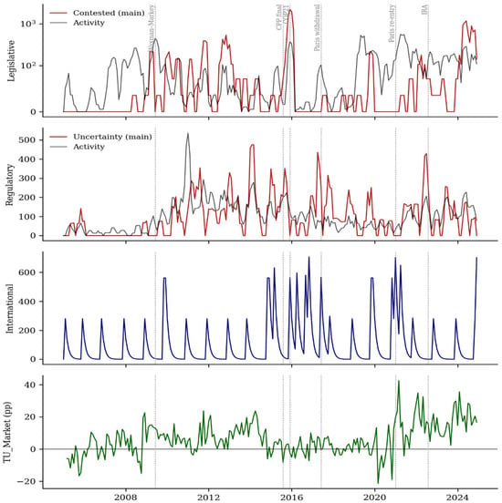
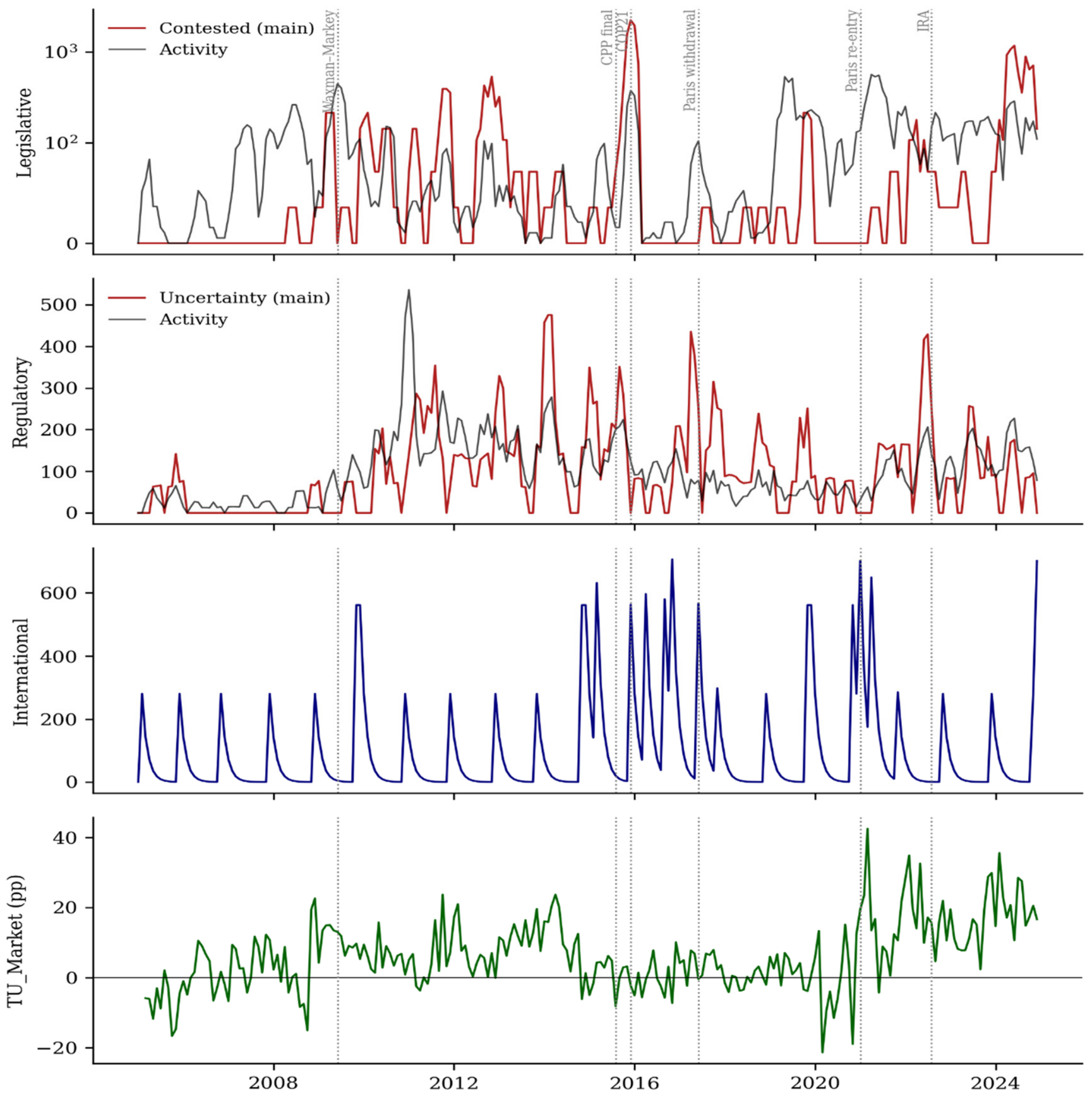
Figure 1 shows why separating uncertainty from activity matters. The contested-legislation index is quiet in most of 2005–2007, and then the Clean Power Plan disapproval battle of late 2015 and the slew of Congressional Review Act resolutions in 2024 take over. The activity index moves on a different rhythm, peaking with Waxman–Markey in 2009 and around the Inflation Reduction Act. Regulatory uncertainty switches on after 2009 and peaks during the 2017 rollback and again in 2022. TU_Market turns persistently positive after 2021, as clean-energy stocks became the riskier side of the transition.

Figure 1. Climate policy uncertainty sub-indices, January 2005–December 2024. Notes: The top two panels compare the uncertainty versions (red) with the activity versions (black) of the legislative and regulatory indices. The legislative panel uses a symmetric log scale. Dotted lines mark Waxman–Markey passage, the final Clean Power Plan, COP21, the Paris withdrawal announcement, Paris re-entry, and the IRA. N = 240.

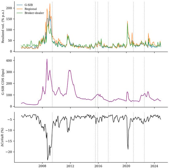
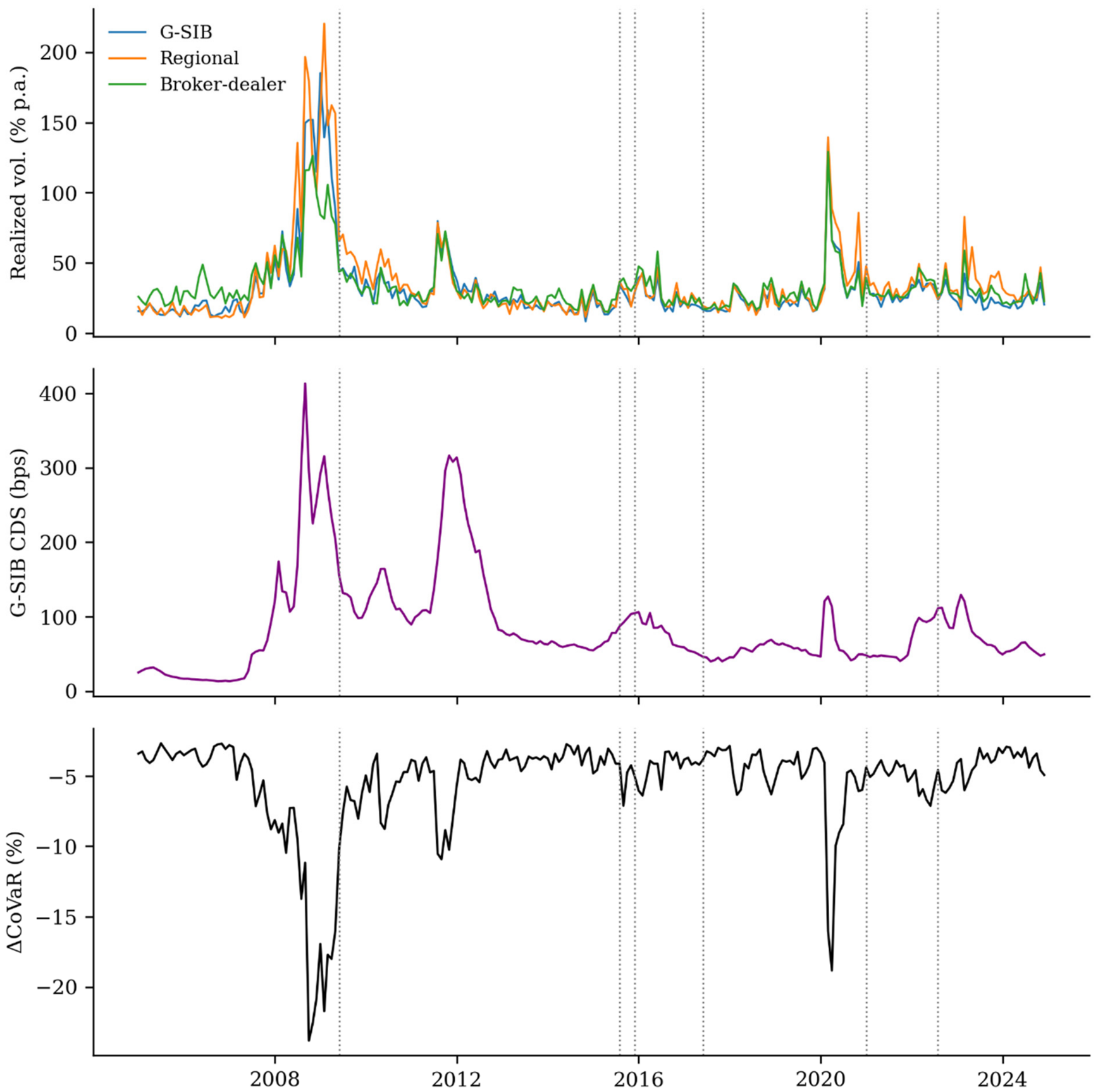
Figure 2 shows that bank risk has its own history. Its largest movements, the 2008–2009 crisis, March 2020, and the regional-bank episode of March 2023, have no climate-policy origin. Any climate-policy signal therefore sits on top of large common shocks, which is why the model works with changes and conditions on macro-financial controls.

Figure 2. Systemic banking risk measures, January 2005–December 2024. Notes: The top panel shows realized equity volatility for G-SIBs, regional banks and broker-dealers; the middle panel shows the average five-year G-SIB CDS spread; the bottom panel shows ΔCoVaR, where more negative values indicate a larger systemic contribution. Dotted lines as in Figure 1. N = 240.

4.2. System-Wide and Net Connectedness Across Market States

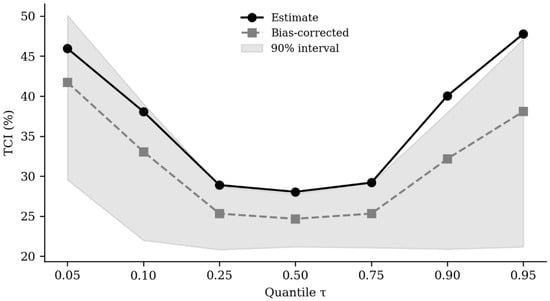
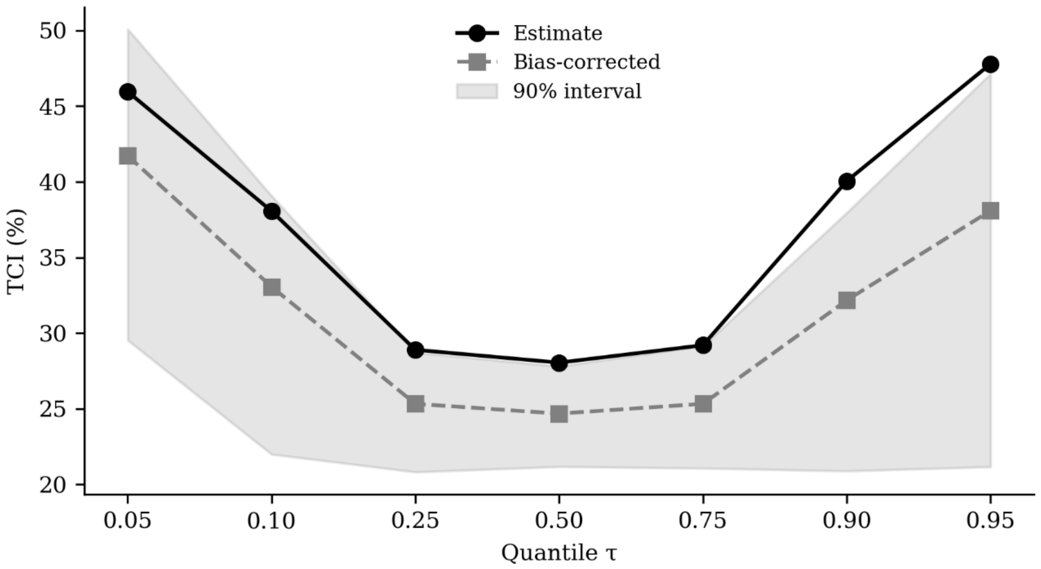
The system is only moderately connected in normal months but becomes markedly more interdependent in distress (Table 6, Figure 3). The finite-sample upward bias of the estimator is excluded, and about 25% of the forecast error variance is actually due to spillovers around the median. The bias correction is important: there is sampling noise that leads to an overestimate of connectedness, particularly in the tails, and so the bias-corrected row is a better indicator of magnitudes.

Table 6. Total and net connectedness by quantile.

	τ = 0.05	τ = 0.10	τ = 0.25	τ = 0.50	τ = 0.75	τ = 0.90	τ = 0.95
TCI, estimate	45.96	38.07	28.90	28.05	29.20	40.05	47.79
TCI, bias-corrected	41.72	33.07	25.33	24.68	25.33	32.17	38.09
TCI, 90% interval	[29.53, 50.09]	[21.99, 39.08]	[20.82, 28.72]	[21.17, 27.81]	[21.07, 29.16]	[20.88, 37.96]	[21.16, 47.14]
NET connectedness
CPU_Legislative	−21.25	−8.38	−0.88	−1.16	−0.67	1.24	1.23
CPU_Regulatory	−15.61	−24.29	2.07	3.64	−5.56	−2.13	6.44
CPU_International	1.00	15.93	2.18	0.69	0.68	−13.99	−25.67
TU_Market	−41.70 †	−24.22	−6.31	−8.88	−2.49	−3.32	−18.70
GSIB_Equity_Risk	−4.98	11.68	13.16 †	9.55	6.84	4.39	11.09
Regional_Equity_Risk	7.23	16.29	7.44	2.98	3.46	−10.61	−3.10
IB_Equity_Risk	−22.11 †	2.90	1.14	5.16	7.03	18.08	5.75
GSIB_CDS_bps	86.39 †	30.61	7.43	7.32	7.59	12.37	25.54
Delta_CoVaR_pct	11.03	−20.53	−26.24 †	−19.31 †	−16.87	−6.03	−2.58

Notes: Values in percent from the QVARX of Equation (1), H = 100. Bias-corrected values equal twice the estimate minus the bootstrap median. Intervals are 90% basic bootstrap intervals from 500 moving-block replications (block length 6). Replications with an eigenvalue modulus of one or more are discarded; valid replications by quantile are 430, 486, 500, 500, 495, 465, and 371. † marks NET values whose interval excludes zero.

Figure 3. Total connectedness index across quantiles. Notes: Black: point estimate. Gray dashed: bias-corrected estimate. Shaded area: 90% basic bootstrap interval. N = 236.

The evidence is clear at the lower tail. At τ = 0.05, the connectedness is above the median, with the 90% interval of the bias-corrected difference being all above zero (difference 17.3 pp, interval [4.9, 24.8]). The upper tail exhibits a comparable point estimate, and an interval that contains zero when noise is considered. When risk is declining rapidly, which typically occurs during the recovery months following a shock, the transmission of issues through climate policy and banking is strongest, while risk at the bank is less precisely measured during and around the time of a shock when it is surging. H2 receives, therefore, only partial support: the amplification of the tail is only supported on one side of the distribution.

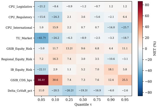
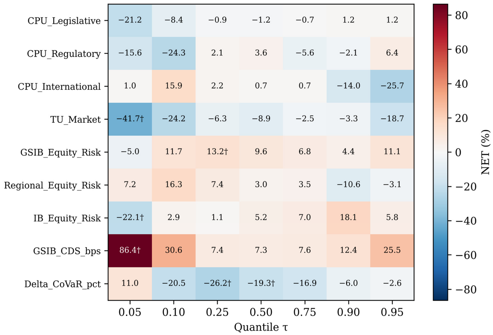
The net measures in Figure 4 say who drives whom. None of the NET values of the policy variables is different from zero, which means that they are net takers of the system at any quantile, taking into account uncertainty. This means that in the lower tail there is a significant net receiver with TU_Market, which is consistent with clean-energy volatility taking a cue from the rest of the system rather than sending it out. There is a general trend of positive net transmission from G-SIB CDS spreads on the lower tail of the banking block and ΔCoVaR as a strong net receiver around the middle of the distribution. Taking the lead from credit markets, the systemic-risk measure follows suit, using ΔCoVaR’s construction from equity returns, which already incorporate news about the credit markets.

Figure 4. NET directional connectedness by variable and quantile. Notes: Red cells denote net transmitters, blue cells net receivers. † marks values whose 90% interval excludes zero. N = 236.

4.3. Which Policy Channel Reaches the Banks?

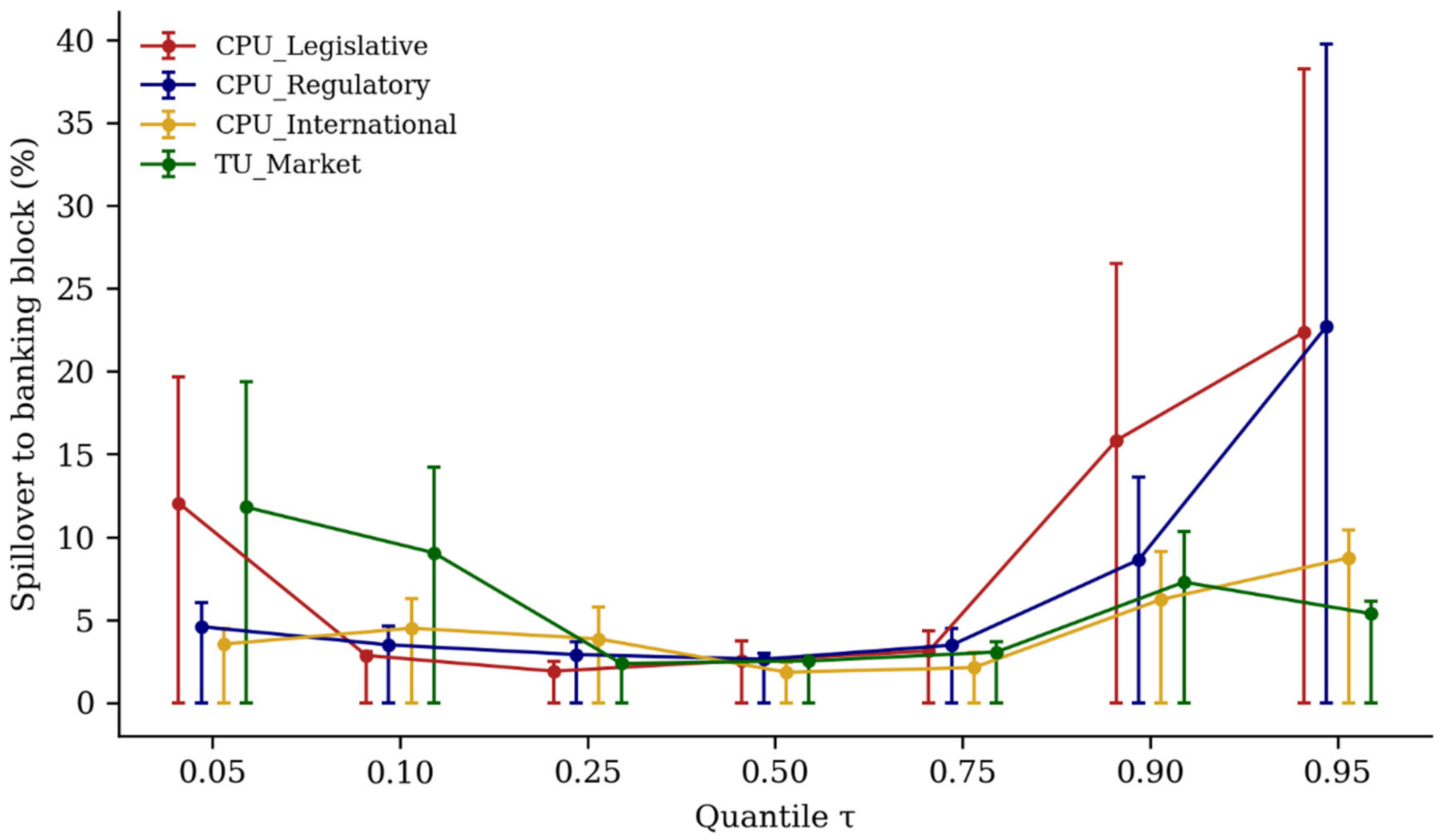
The block spillover in Equation (4) isolates the question that matters for supervisors: how much of the variation in bank risk can be traced to each policy channel (Table 7, Figure 5)? Near the median, the answer is very little. Each sub-index accounts for a few percent of the banking block’s forecast error variance, and none of these shares is distinguishable from the noise level that the bias correction implies. In ordinary months, climate policy uncertainty does not move U.S. bank risk in any measurable way once market fear, general policy uncertainty, monetary conditions, and the credit cycle are controlled for.

Table 7. Spillovers from each policy variable to the banking block.

Policy Variable	τ = 0.05	τ = 0.10	τ = 0.25	τ = 0.50	τ = 0.75	τ = 0.90	τ = 0.95
CPU_Legislative	12.05	2.86	1.91	2.54	3.12	15.83	22.37
90% interval	[0.00, 19.66]	[0.00, 3.09]	[0.00, 2.51]	[0.00, 3.72]	[0.00, 4.36]	[0.00, 26.52]	[0.00, 38.25]
CPU_Regulatory	4.59	3.49	2.91	2.63	3.47	8.63	22.71
90% interval	[0.00, 6.06]	[0.00, 4.63]	[0.00, 3.70]	[0.00, 3.00]	[0.00, 4.47]	[0.00, 13.62]	[0.00, 39.72]
CPU_International	3.54	4.50	3.86	1.85	2.12	6.24	8.75
90% interval	[0.00, 4.50]	[0.00, 6.30]	[0.00, 5.80]	[0.00, 2.45]	[0.00, 3.04]	[0.00, 9.13]	[0.00, 10.45]
TU_Market	11.80	9.05	2.37	2.53	3.06	7.28	5.37
90% interval	[0.00, 19.36]	[0.00, 14.23]	[0.00, 2.34]	[0.00, 2.77]	[0.00, 3.68]	[0.00, 10.31]	[0.00, 6.11]

Notes: Entries are TO_k → B from Equation (4): the summed share (%) of the five banking variables’ forecast error variance attributable to policy variable k, with a maximum of 500. Intervals are 90% basic bootstrap intervals, truncated at zero. Because basic intervals are centered on the bias-corrected value, an upper bound can fall below the raw estimate when the estimated bias is large. At τ = 0.95, the supervisory spillover surpasses the international (difference 13.96, interval [0.58, 72.63]) and TU_Market (17.33, [1.94, 70.40]) spillovers; no other pairwise variance is substantial.

Figure 5. Spillovers from each policy variable to the banking block, by quantile. Notes: Markers show point estimates; bars show 90% basic bootstrap intervals truncated at zero. N = 236.

The tails tell a different story. At τ = 0.95, both the legislative and the regulatory channels carry spillovers roughly eight times their median values. Regulatory uncertainty is the only channel whose upper-tail spillover is significantly larger than that of other channels: it exceeds both international-commitment uncertainty and TU_Market. It cannot be separated from legislative uncertainty, however, though the regulatory channel proves the more robust of the two (Section 4.8). In the lower tail, the legislative channel and TU_Market carry the largest point estimates, but with wide intervals.

The regulatory channel therefore matters most when bank risk is rising fastest, and on that point H1 survives. But it does not dominate across market states, and contested legislation is as important in the same tail. H1 holds only in this narrower form.

4.4. Horizons

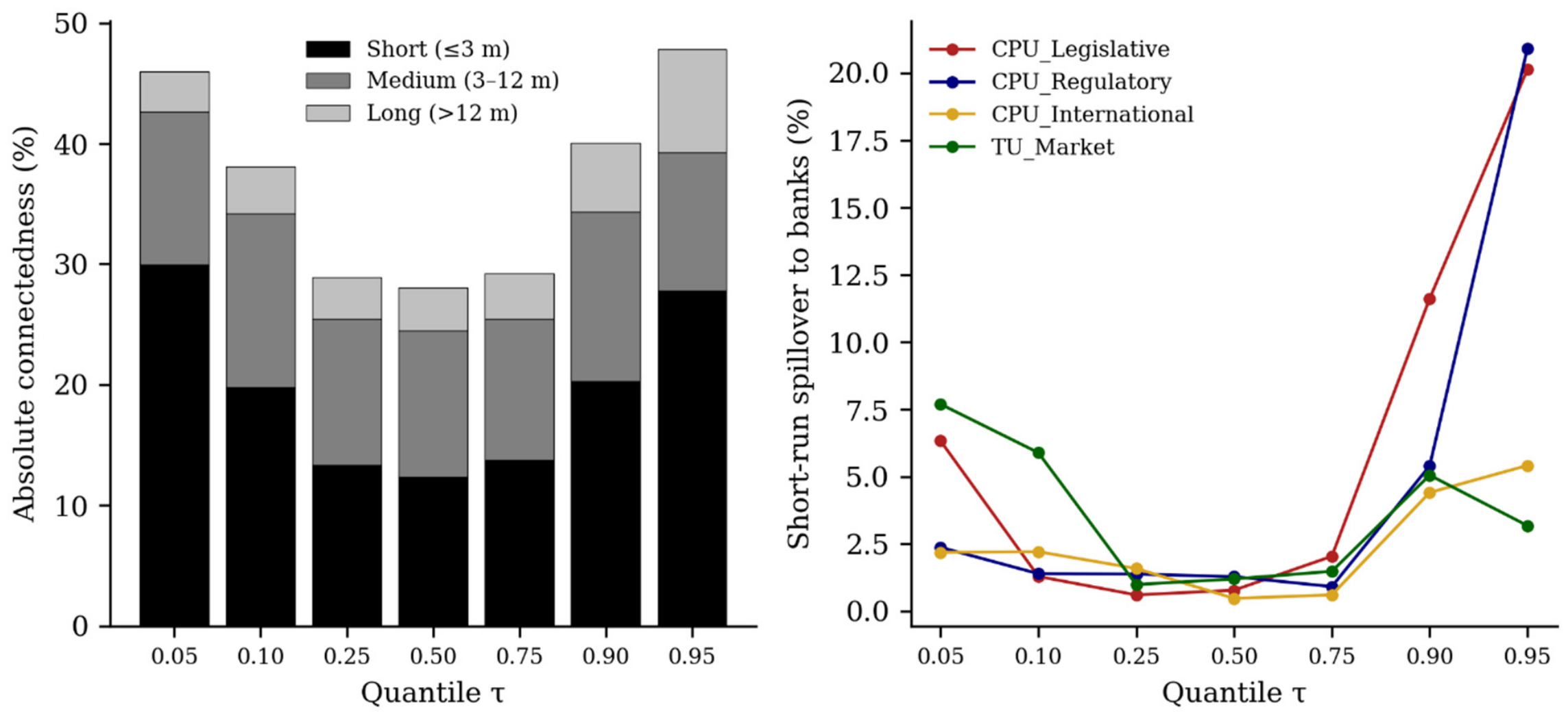
Most connectedness in this system is short- and medium-run (Table 8, Figure 6). Cycles longer than a year account for a small part of total connectedness at every quantile, even though within that band the variables are reasonably well connected. The two band measures answer different questions, and they now reconcile exactly: absolute contributions sum to the TCI, and band weights sum to 100.

Table 8. Frequency decomposition of connectedness. Panel A: Band Connectedness. Panel B. Spillovers from each policy variable to the banking block, by band.

Panel A: Band Connectedness
τ		Band		Absolute C_d		Within C^W_d		Weight w_d (%)
0.05		Short (≤3 m)		29.98 [8.85, 41.19]		59.09 [44.39, 70.83]		50.73 [32.01, 63.34]
0.05		Medium (3–12 m)		12.68 [4.03, 18.12]		36.11 [23.90, 40.74]		35.10 [23.79, 49.06]
0.05		Long (>12 m)		3.31 [0.00, 4.63]		23.33 [0.00, 20.82]		14.17 [6.74, 21.51]
0.05		Sum/TCI		45.96		–		100.00
0.50		Short (≤3 m)		12.38 [7.32, 13.14]		31.35 [21.89, 31.57]		39.47 [35.18, 42.52]
0.50		Medium (3–12 m)		12.13 [8.71, 13.22]		27.12 [20.58, 27.96]		44.72 [42.10, 48.58]
0.50		Long (>12 m)		3.54 [1.86, 3.93]		22.42 [13.73, 23.63]		15.81 [14.10, 17.46]
0.50		Sum/TCI		28.05		–		100.00
0.95		Short (≤3 m)		27.83 [0.00, 37.79]		52.31 [24.77, 56.47]		53.20 [29.81, 71.41]
0.95		Medium (3–12 m)		11.43 [0.35, 17.23]		40.48 [22.98, 40.11]		28.24 [14.79, 44.28]
0.95		Long (>12 m)		8.54 [0.00, 14.12]		45.99 [18.29, 55.75]		18.56 [2.41, 29.83]
0.95		Sum/TCI		47.79		–		100.00
Panel B: Spillovers from each policy variable to the banking block, by band
τ	Band		CPU_Leg → banks		CPU_Reg → banks		CPU_Int → banks		TU_Mkt → banks
0.05	Short (≤3 m)		6.33 [0.00, 11.49]		2.38 [0.00, 3.98]		2.19 [0.00, 3.48]		7.69 [0.00, 12.98]
0.05	Medium (3–12 m)		4.37 [0.00, 7.69]		1.94 [0.00, 2.98]		1.03 [0.00, 1.34]		3.75 [1.29, 6.78]
0.05	Long (>12 m)		1.35 [0.00, 2.39]		0.27 [0.00, 0.39]		0.32 [0.00, 0.50]		0.36 [0.00, 0.64]
0.50	Short (≤3 m)		0.78 [0.00, 1.15]		1.29 [0.00, 1.70]		0.48 [0.00, 0.55]		1.20 [0.00, 1.41]
0.50	Medium (3–12 m)		1.09 [0.00, 1.67]		1.06 [0.00, 1.28]		0.95 [0.00, 1.41]		0.90 [0.00, 1.25]
0.50	Long (>12 m)		0.67 [0.00, 1.24]		0.29 [0.00, 0.44]		0.42 [0.00, 0.72]		0.43 [0.00, 0.77]
0.95	Short (≤3 m)		20.13 [0.00, 38.20]		20.92 [0.48, 39.57]		5.42 [0.00, 8.80]		3.18 [0.00, 4.46]
0.95	Medium (3–12 m)		1.81 [0.00, 2.73]		1.29 [0.00, 1.87]		2.55 [0.00, 3.87]		1.67 [0.00, 2.62]
0.95	Long (>12 m)		0.43 [0.00, 0.60]		0.50 [0.00, 0.86]		0.79 [0.00, 1.28]		0.52 [0.00, 0.87]

Notes: Absolute and within-band connectedness follow Equations (6) and (7); weights w_d are band variance shares. Short, medium and long bands correspond to ω ∈ (2π/3, π], (π/6, 2π/3] and [0, π/6]. Brackets show 90% basic bootstrap intervals, truncated at zero. The final four columns apply Equation (4) to the band decomposition. Results for τ = 0.10 and 0.90 are available in the replication files.

Figure 6. Frequency decomposition across quantiles. Notes: (Left): absolute band contributions to the TCI (they sum to the TCI at each quantile). (Right): short-run spillovers from each policy variable to the banking block. N = 236.

Policy spillovers to banks are concentrated at short horizons, especially in the tails. At τ = 0.95, the short-run spillovers from legislative and regulatory uncertainty make up almost all of their tail transmission, and the regulatory short-run spillover is the only band-level policy spillover whose interval excludes zero. This is the reverse of H3, which expected regulatory uncertainty to work mainly through medium-run rulemaking cycles. Banks appear to reprice regulatory reversal risk within a quarter of the news, not over the months that a rule takes to work through the Federal Register. The medium-run spillovers of all four channels are small and similar in size.

4.5. Rising Versus Falling Uncertainty

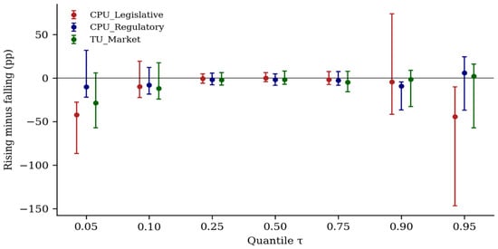
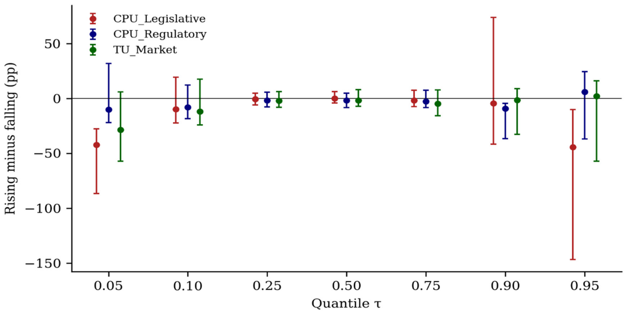
H4: Expected uncertainty increases to pass through more strongly than was expected during the uncertainty decreases. Where the other data went (Table 9, Figure 7). Close to the median, uncertainty increases and decreases the same way for all three channels. Even at τ = 0.05 and τ = 0.95, the contribution of months with increasing contested-legislation uncertainty to the variation in bank-risk is significantly lower than the contribution of months with decreasing contested-legislation uncertainty in the tails. This is also the case with regulatory uncertainty at τ = 0.90.

Table 9. Asymmetric spillovers: rising versus falling uncertainty.

τ	Leg: Rising	Leg: Falling	Leg: Asymmetry	Reg: Rising	Reg: Falling	Reg: Asymmetry	TU: Rising	TU: Falling	TU: Asymmetry
0.05	2.58	44.99	−42.41 † [−86.72, −27.78]	1.35	11.35	−10.00 [−22.04, 31.93]	4.66	33.33	−28.67 [−57.19, 6.05]
0.10	1.81	11.75	−9.94 [−22.43, 19.29]	1.41	9.34	−7.93 [−18.42, 12.25]	4.54	16.52	−11.98 [−24.10, 17.61]
0.25	2.41	2.99	−0.58 [−5.99, 4.72]	1.55	3.20	−1.65 [−7.78, 5.77]	1.88	3.86	−1.98 [−8.10, 6.35]
0.50	2.12	2.19	−0.07 [−4.23, 6.30]	1.06	2.74	−1.68 [−8.26, 4.63]	3.13	4.79	−1.66 [−7.15, 8.20]
0.75	1.91	3.79	−1.88 [−7.37, 7.45]	0.50	3.15	−2.65 [−8.28, 7.58]	2.93	7.82	−4.90 [−15.68, 7.81]
0.90	12.08	16.60	−4.52 [−41.65, 74.00]	2.84	12.21	−9.37 † [−36.50, −4.38]	8.54	9.96	−1.42 [−32.75, 9.07]
0.95	38.54	82.84	−44.30 † [−146.68, −10.01]	18.33	12.22	6.11 [−36.78, 24.49]	6.66	4.54	2.12 [−57.16, 16.06]

Notes: “Rising” and “falling” are TO_k→B from systems based on the positive and negative components of each policy variable (Equation (8)), and asymmetry is as given in Equation (9). Basic bootstrap intervals are indicated by brackets and intervals that do not contain the value 0 are marked with †. Replications with any system eigenvalue equal to or greater are excluded—an acceptable range of replications is 196 (τ = 0.95) to 500 (τ = 0.25, 0.50).

Figure 7. Asymmetry in spillovers to the banking block (rising minus falling uncertainty). Notes: Markers show point estimates; bars show 90% basic bootstrap intervals. Negative values mean falling uncertainty transmits more than rising uncertainty. N = 236.

For this reason, the decrease in values in these indices is not a random ‘quiet’ month. They signal the end of contestation episodes: a veto that’s successful and brings an end to a disapproval battle, a rule challenged and which survives, and a stay by the Supreme Court. As for our reading, resolution is a much greater concern than any outbreak of conflict; it addresses the policy trajectory and against which bank exposures will then need to be priced. The comparison is between an increasing situation of uncertainty and a decreasing situation of uncertainty, not necessarily whether the one is more or less dangerous for banks. In the extreme tails, there are lower numbers of valid replications, and thus the asymmetries are less well-estimated than the median results.

4.6. Transmission over Time

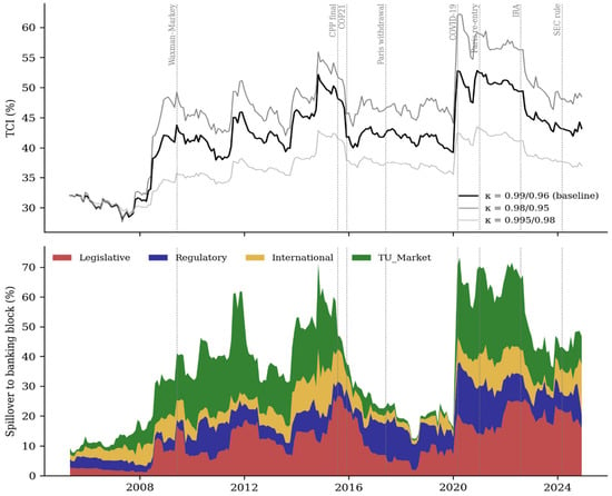
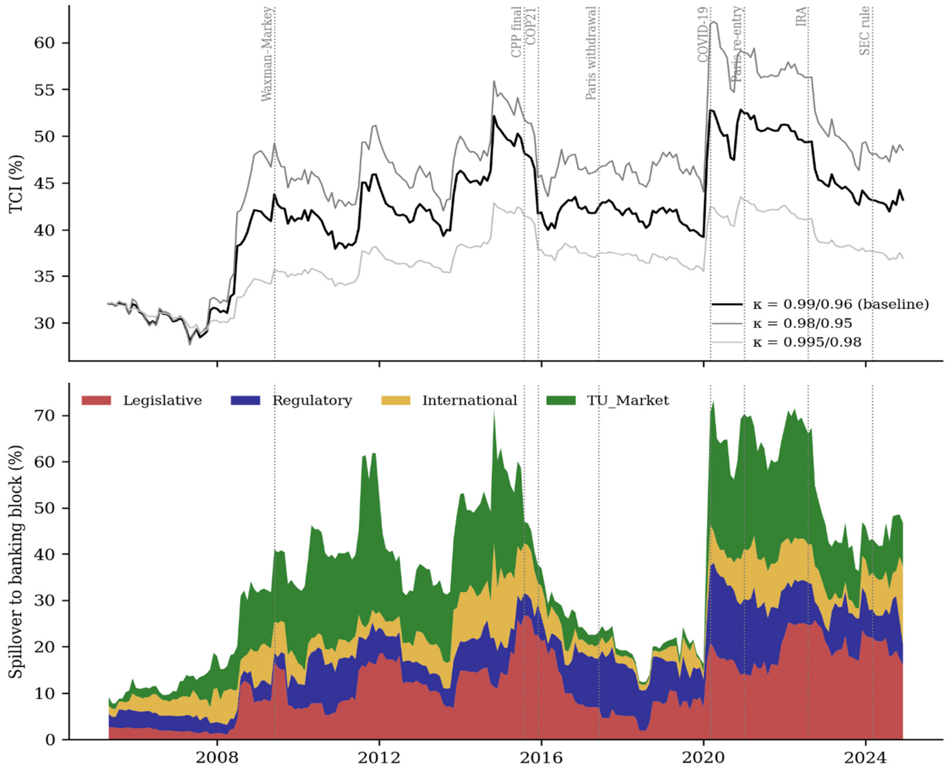
In Figure 8, the time-varying estimates indicate a turnabout of the channels. Legislative spillovers to banks increase following the Clean Power Plan disapproval votes (2015) and increase again for banking-agency disapproval resolutions (2022). Regulatory spillovers are highest during the 2017–2018 rollback period and during the 2020–2021 shift between administrations when the Federal Register is filled with regulatory ‘stays,’ reconsiderations, and repeals. TU_Market shares are highest during 2010–2015 and after 2020, when shares are the most volatile in the clean-energy component.

Figure 8. Time-varying connectedness from the TVP-VARX. Notes: (Top): total connectedness under three forgetting-factor pairs. (Bottom): spillovers from each policy variable to the banking block (baseline factors 0.99/0.96), stacked. Dotted lines mark policy events and COVID-19. May 2005–December 2024, N = 236.

The financial crisis moves system connectedness forward, reaching a high level in 2015 and rising anew in 2020–2021, only to drop following 2022. The pattern is identical for all three combinations of forgetting factors. The filter starts with OLS estimates with the full sample, and therefore no observations are lost, starting in May 2005. This view of the changing channels, rather than having one channel prevailing all the way around, corresponds with the results of the full sample quantile analysis.

4.7. Event Windows

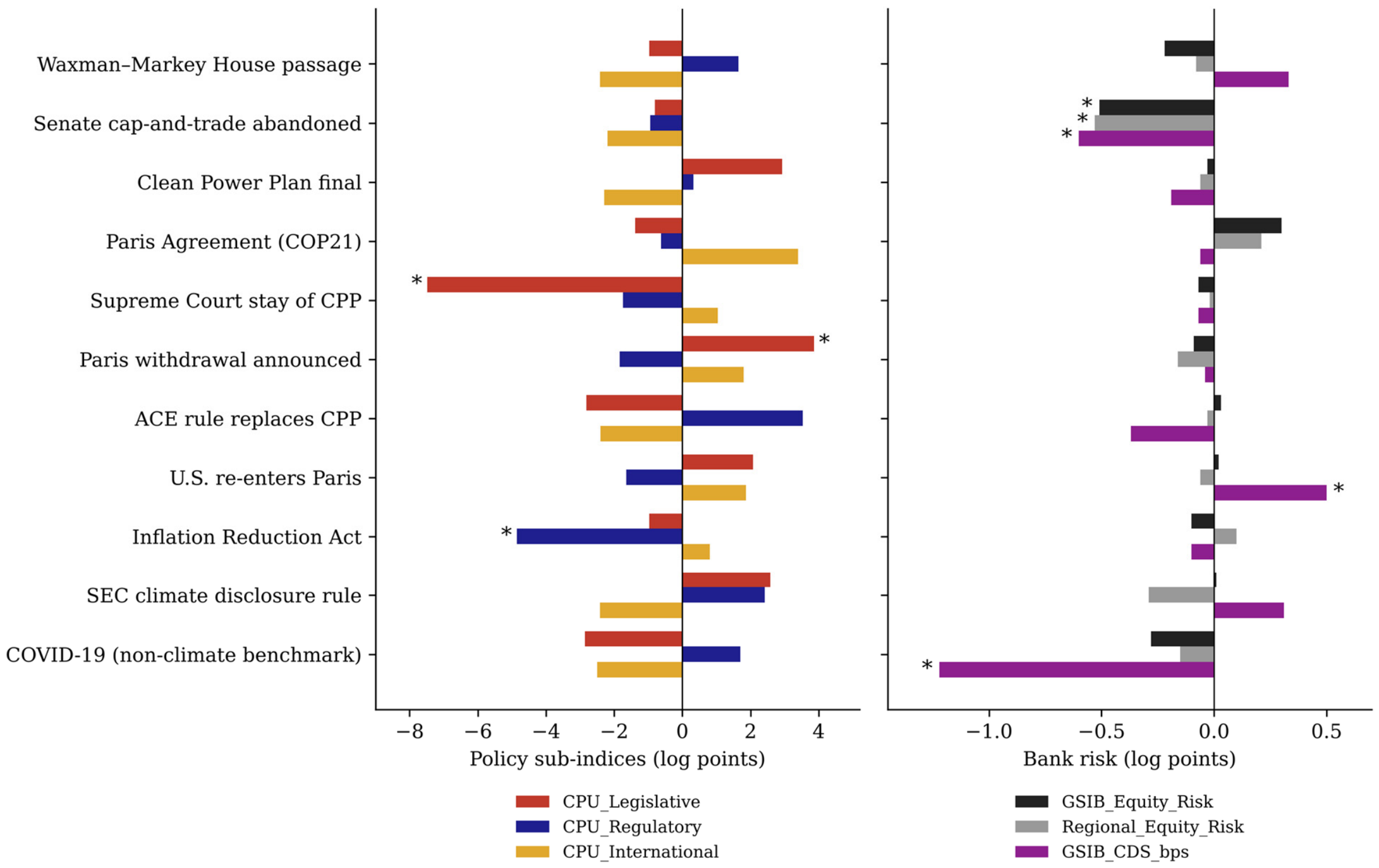
Table 10 and Figure 9 show the movements of the variables around the identified episodes, after the effect of the lagged controls has been removed. As their construction suggests, so do the policy indices respond. After the Supreme Court’s stay of the Clean Power Plan, the contested-legislation index drops precipitously. The measure of regulatory uncertainty is greatest when the Affordable Clean Energy rule replaces the Clean Power Plan, and decreases after the IRA. TU_Market rises when the U.S. re-enters Paris, and drops during COVID-19. Two answers that sound paradoxical will naturally ensue from the way the indices are calculated. The withdrawal announcement in Paris is counted as a change in the commitment of the USA: it marked a time of uncertainty about the U.S. commitment. Deregulation likewise raises regulatory uncertainty in our measure, because stays, reconsiderations, and repeal notices are what the index counts. Table 2 shows the regulatory index far above its activity counterpart throughout the 2017 rollback. Around June 2017, the pre- and post-event windows both fall inside that elevated period, so the event difference is small.

Table 10. Control-adjusted event-window changes (±3 months). Panel A. Policy Variables. Panel B. Banking risk variables.

Panel A. Policy Variables
Event (Month)		CPU_Leg		CPU_Reg		CPU_Int		TU_Mkt
Waxman–Markey House passage (June 2009)		−0.97 [−5.06, 2.44]		1.65 [−1.52, 5.12]		−2.42 [−6.07, 0.72]		−6.57 [−22.08, 5.89]
Senate cap-and-trade abandoned (July 2010)		−0.80 [−4.44, 2.56]		−0.94 [−4.26, 2.72]		−2.19 [−6.11, 0.63]		−1.17 [−13.67, 9.77]
Clean Power Plan final (August 2015)		2.92 [−0.32, 6.13]		0.33 [−3.02, 3.66]		−2.29 [−6.59, 0.37]		−2.32 [−14.62, 9.91]
Paris Agreement, COP21 (December 2015)		−1.38 [−5.24, 2.49]		−0.62 [−4.01, 2.75]		3.40 [−0.29, 6.75]		−4.87 [−20.56, 9.32]
Supreme Court stay of CPP (February 2016)		−7.48 † * [−10.84, −4.03]		−1.74 [−5.17, 1.64]		1.04 [−3.03, 3.74]		−0.67 [−12.77, 11.66]
Paris withdrawal announced (June 2017)		3.86 * [−0.22, 7.74]		−1.84 [−5.24, 1.60]		1.80 [−1.97, 5.02]		1.54 [−13.40, 15.39]
ACE rule replaces CPP (June 2019)		−2.82 [−6.75, 0.97]		3.53 † [0.28, 6.98]		−2.40 [−6.16, 0.87]		−2.11 [−16.79, 12.33]
U.S. re-enters Paris (January 2021)		2.07 [−1.43, 5.47]		−1.65 [−5.08, 1.92]		1.86 [−2.15, 4.52]		26.11 † * [14.30, 37.00]
Inflation Reduction Act (August 2022)		−0.97 [−4.23, 2.56]		−4.85 † * [−8.05, −1.45]		0.81 [−3.52, 3.52]		−5.28 [−17.75, 5.57]
SEC climate disclosure rule (March 2024)		2.58 [−0.99, 6.50]		2.41 [−0.92, 5.82]		−2.42 [−6.26, 0.74]		−11.34 * [−25.60, 3.46]
COVID-19, non-climate benchmark (March 2020)		−2.85 [−6.33, 0.87]		1.70 [−1.56, 4.99]		−2.50 [−5.92, 0.68]		−19.88 † * [−33.91, −5.07]
Panel B. Banking risk variables
Event (month)	GSIB_Eq		Reg_Eq		IB_Eq		GSIB_CDS		ΔCoVaR
Waxman–Markey House passage (June 2009)	−0.22 [−0.69, 0.19]		−0.08 [−0.64, 0.39]		−0.21 [−0.62, 0.13]		0.33 [−0.44, 1.20]		4.34 † * [1.92, 7.38]
Senate cap-and-trade abandoned (July 2010)	−0.51 † * [−0.89, −0.06]		−0.53 † * [−1.01, −0.06]		−0.25 [−0.61, 0.13]		−0.60 † * [−1.16, −0.04]		2.23 * [−0.38, 4.38]
Clean Power Plan final (August 2015)	−0.03 [−0.46, 0.38]		−0.06 [−0.54, 0.38]		0.18 [−0.22, 0.57]		−0.19 [−0.75, 0.43]		0.98 [−1.43, 3.52]
Paris Agreement, COP21 (December 2015)	0.30 [−0.12, 0.74]		0.21 [−0.31, 0.75]		0.12 [−0.25, 0.52]		−0.06 [−0.87, 0.76]		0.10 [−2.63, 2.78]
Supreme Court stay of CPP (February 2016)	−0.07 [−0.52, 0.40]		−0.02 [−0.51, 0.45]		−0.06 [−0.43, 0.34]		−0.07 [−0.64, 0.56]		0.34 [−2.67, 3.01]
Paris withdrawal announced (June 2017)	−0.09 [−0.51, 0.35]		−0.16 [−0.70, 0.35]		−0.23 [−0.65, 0.14]		−0.04 [−0.90, 0.77]		0.32 [−2.21, 3.18]
ACE rule replaces CPP (June 2019)	0.03 [−0.39, 0.48]		−0.03 [−0.56, 0.48]		0.08 [−0.30, 0.49]		−0.37 [−1.20, 0.46]		−0.29 [−3.25, 2.29]
U.S. re-enters Paris (January 2021)	0.02 [−0.36, 0.46]		−0.06 [−0.56, 0.42]		−0.01 [−0.39, 0.37]		0.50 * [−0.06, 1.07]		−0.46 [−3.36, 1.66]
Inflation Reduction Act (August 2022)	−0.10 [−0.52, 0.36]		0.10 [−0.38, 0.54]		−0.06 [−0.43, 0.32]		−0.10 [−0.69, 0.51]		0.27 [−2.23, 2.72]
SEC climate disclosure rule (March 2024)	0.01 [−0.43, 0.43]		−0.29 [−0.79, 0.21]		−0.10 [−0.49, 0.28]		0.31 [−0.50, 1.15]		−0.60 [−3.08, 1.95]
COVID-19, non-climate benchmark (March 2020)	−0.28 [−0.68, 0.13]		−0.15 [−0.65, 0.35]		0.03 [−0.33, 0.39]		−1.22 † * [−2.12, −0.36]		−0.79 [−3.34, 1.63]

Notes: Each entry is the mean residual over the three months after the event month minus the mean over the three months before, with residuals from a full-sample regression on the lagged controls. CPU indices are in log(1 + x) points, equity risk and CDS in log points, TU_Market in percentage points, and ΔCoVaR in percent; the sample standard deviation of ΔCoVaR is 3.48. Brackets show 90% residual block-bootstrap intervals (2000 replications, six-month blocks); † marks intervals that exclude zero. * marks changes outside the 5th–95th percentile range of 161 placebo windows centered on non-event months.

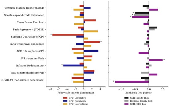
Figure 9. Event-window changes in policy sub-indices and bank risk. Notes: Bars show control-adjusted changes (±3 months) from Table 10; * marks changes outside the placebo 5th–95th percentile range. N = 236.

Bank risk rarely moves around climate events. Equity and CDS responses are small and, with one exception, indistinguishable from zero under both the bootstrap intervals and the placebo range. The exception is July 2010, when the Senate abandoned cap-and-trade and equity risk, and CDS spreads eased. ΔCoVaR shows the two largest movements, in June 2009 and July 2010, of roughly 1.2 and 0.6 standard deviations. These are economically large reductions in systemic contribution. However, they coincide with the publication of the bank stress-test results in May 2009 and with the passage of the Dodd–Frank Act and the calming of the European sovereign crisis in July 2010, so they cannot be attributed to the climate decisions. Every other ΔCoVaR change is below a third of a standard deviation, small in economic terms and statistically indistinguishable from zero. The COVID-19 benchmark shows the scale of a genuine macro-financial shock. Taken with Section 4.2 and Section 4.3, the event evidence agrees that climate policy events leave little trace on bank risk in normal conditions. The exercise is descriptive and, as Section 3.8 explains, cannot establish that any observed change was caused by the policy event.

4.8. Robustness

Table 11 re-estimates the system under alternative choices. The horizon makes no difference. The reduction of the controls leads to an increase in the upper tail connectedness and the upper tail spillover of the legislation, indicating that part of the raw TAW is due to the common macro-financial conditions.

Table 11. Robustness of connectedness and policy spillovers.

Specification	TCI τ = 0.05	TCI τ = 0.50	TCI τ = 0.95	Leg → Banks 0.05/0.50/0.95	Reg → Banks 0.05/0.50/0.95	Int → Banks 0.05/0.50/0.95	TU → Banks 0.05/0.50/0.95
Baseline	45.96	28.05	47.79	12.05/2.54/22.37	4.59/2.63/22.71	3.54/1.85/8.75	11.80/2.53/5.37
Two lags (AIC)	48.64	28.86	60.33	14.66/4.00/53.17	24.01/4.62/16.55	10.62/8.78/50.77	6.47/4.77/16.13
H = 12	45.96	28.05	47.67	12.05/2.54/22.29	4.59/2.63/22.57	3.54/1.85/8.68	11.80/2.53/5.37
No controls	42.01	27.91	56.69	10.99/2.04/31.29	4.67/1.65/19.04	7.27/3.09/13.72	9.47/2.29/2.78
Activity versions of narrative indices	43.56	27.84	42.02	2.30/0.81/2.26	15.73/2.80/13.18	3.72/3.03/9.89	8.27/3.01/6.05
Full-text regulatory index	43.23	28.09	54.40	11.17/2.21/9.42	4.18/1.69/12.48	3.05/3.08/18.94	13.41/2.81/7.22
Adding oil prices and geopolitical risk	50.35	27.75	43.58	11.74/2.60/12.15	9.26/1.59/18.06	3.17/1.82/11.26	11.21/2.27/6.16

Notes: Point estimates in percent. In the activity row, CPU_Legislative_Activity and CPU_Regulatory_Activity replace the uncertainty versions; in the full-text row, CPU_Regulatory_FullText replaces CPU_Regulatory. All other settings are the same as baseline. Additional lagged controls are added to the final row, including monthly log changes in the price of West Texas crude oil (FRED, MCOILWTICO) and a log of the Caldara and Iacoviello [64] geopolitical risk index.

Two checks are directly relevant to the measurement argument of the paper. Replacing the contested legislative index with the activity version removes almost all legislative transmission to banks at every quantile. Bank risk responds to fights over climate legislation, not to the volume of climate bills, which is the strongest evidence that the filter captures something economically meaningful. Replacing the regulatory uncertainty index with its activity or full-text versions shifts transmission toward the lower tail and weakens the upper-tail regulatory spillover; the upper-tail regulatory result of Section 4.3 therefore depends on the uncertainty filter.

To test for omitted common drivers, we add monthly oil-price changes and the geopolitical risk index of Caldara and Iacoviello [64] as further lagged controls. Median connectedness and the lower-tail spillovers barely move. In the upper tail, the legislative spillover roughly halves while the regulatory spillover changes much less, so regulatory reversal risk becomes the largest channel when bank risk rises fastest. Part of the upper-tail legislative transmission therefore coincides with energy and geopolitical shocks, whereas the regulatory channel is not explained by them. The lower-tail pattern, in which contested legislation and TU_Market carry the largest spillovers, is unaffected.

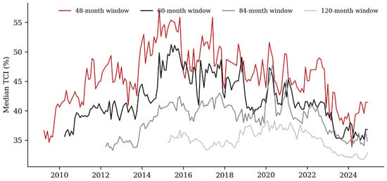
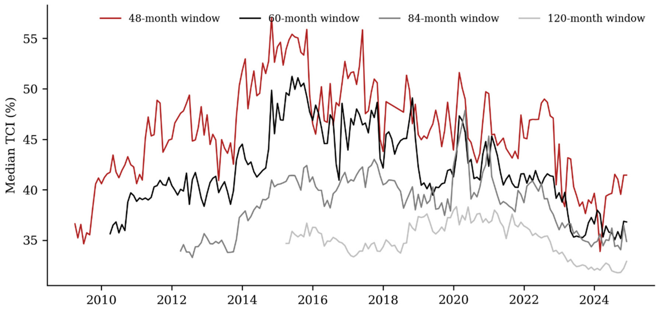
The two-lag model magnifies tail transmission through each channel and causes the international channel to be large in the upper tail. This specification enhances the equations with 9 additional slope parameters for each equation, and as a result, its tail estimates are less reliable because of the high cost in the tails. The picture of level and timing is the same as in the rolling median estimates (Figure 10). In all window sizes, connectedness increases from 2014–2016 and also around 2020–2021, but decreases with window size, from approximately 39–52% for the 48-month window to 32–37% for the 120-month window. This ordering is precisely the one suggested by the finite-sample bias reported in Section 3.5.4: with shorter windows, there will be fewer observations per parameter and more spurious spillovers. This results in the shortest time window producing the most explosive estimates, which are set aside.

Figure 10. Rolling-window median connectedness. Notes: TCI at τ = 0.50 from QVARX models re-estimated in rolling windows of 48, 60, 84 and 120 months, plotted at window end. Windows with an eigenvalue modulus of one or more are omitted: ten of 189 at 48 months, one of 177 at 60 months and five of 153 at 84 months. A 24-month window is not reported because each equation has 15 parameters. N = 236.

5. Discussion

The results qualify much of what earlier work has led us to expect. Luna Mallea [8] finds that climate policy uncertainty tightens U.S. credit conditions through the excess bond premium, and Kapetanakis et al. [9] link it to lower profitability and higher instability among large U.S. banks. Both studies rely on a single aggregate index. Our sub-indices show almost no spillover to bank risk in ordinary months once market fear, general policy uncertainty, and the credit cycle are controlled for. Aggregate indices move with broad uncertainty, and part of what they attribute to climate policy may belong to that common component. Climate policy uncertainty has a significant impact only in the tails if measured in terms of reversal risk. Since at the upper tail this is not the only type of risk that is of concern to the regulators, and the international and market channels are also at risk of regulatory reversal, the H1 is true only in this limited way.

However, the evidence related to tail amplification is weaker than the evidence found in the quantile connectedness literature. Both studies, by Chatziantoniou et al. [46] and Hachicha et al. [42], find a significant rise in connectedness at extreme quantiles for the green bond market, as well as equity and commodity markets. The same pattern prevails before accounting for finite-sample bias, but not after that! The more regressions are done from the tail, the fewer the observations are; the more noise is introduced in the sample, the more noise is introduced in the spurious spillovers, and the larger the inflation, the closer the regression is to the region where tail effects are normally reported. It is possible that some of this earlier amplification has been exaggerated and that H2 is on one side of the distribution only.

The asymmetry result is counter to H4, and is consistent with some previous evidence. Zhu et al. [23] conclude that positive CPU shocks outweigh negative shocks, while Güngör [16] reveals that reducing CPU leads to a larger reduction in returns on green bonds than an increase. Rising contestation is a less significant factor in explaining bank risk variability in our tails, while falling contestation is a more significant factor. Resolution, rather than initiation of conflict, may be when deferred decisions are made and exposures repriced: a veto, a court stay, or a failure to vote for a disapproval, and real-options reasoning [52]. H4 assumed banks reprice when uncertainty arrives; our results suggest they wait until it clears.

The frequency results sit closer to Abdu and Alruwaitee [49] and Chen et al. [48], who report short-run dominance and rapid decay. Policy spillovers to banks are concentrated within a quarter, the regulatory channel included. H3 rested on the multi-quarter clock of Federal Register rulemaking, but markets appear to price reversal risk when it becomes visible, not across the administrative life of a rule.

Finally, legislative transmission disappears when contested bills are replaced with the volume of all climate bills. To our knowledge, this distinction between legislative activity and contestation has not been drawn in this literature. What matters for banks, in practice, is less how much climate policy is being made than whether existing policy is likely to survive.

6. Conclusions

The U.S. banking system sits where three streams of climate policy meet: congressional legislation, federal rulemaking and international treaty commitments. The financial stability literature has mostly treated climate policy uncertainty as a single index, which cannot show which of these streams matters for banks or when. The question also matters for sustainability, because banks provide much of the long-term credit needed for the low-carbon transition, and a banking system unsettled by policy swings is less able to supply it. This study separates them. Using 240 monthly observations from January 2005 to December 2024, we build legislative and regulatory indices that count formal attempts to block, delay, or reverse existing climate policy, an index of international commitment events and a market-based measure of transition uncertainty, and we trace their spillovers to five measures of U.S. systemic banking risk with a quantile VAR, a frequency decomposition, a time-varying model and bias-corrected bootstrap inference.

Four main findings stand out. First, climate policy uncertainty leaves little measurable trace on bank risk in ordinary months once market fear, general policy uncertainty, monetary conditions, and the credit cycle are accounted for. Its spillovers appear in the tails of the distribution, and the system as a whole becomes more connected mainly when bank risk is falling sharply. Second, no single channel dominates. Regulatory reversal risk carries more weight than the international and market channels when bank risk is rising fastest, but contested legislation matters just as much, and the weight of each channel shifts from one policy regime to the next. Third, transmission is fast. Spillovers to banks are concentrated within a quarter, the regulatory channel included, so markets appear to price reversal risk when it becomes visible, not over the life of a rule. Fourth, the end of a policy fight matters more than its start. In the tails, falling contestation explains more of the variation in bank risk than rising contestation, and legislative spillovers vanish when contested bills are replaced by the volume of all climate bills. For banks, what matters is whether existing policy survives, not how much policy is being made.

These results carry several implications for supervisors. Climate stress scenarios built on average responses to climate-policy news will understate risk in the states that matter, because the relevant transmission occurs in the tails. Scenarios should therefore be designed around contestation episodes, such as disapproval campaigns, litigation that stays a rule, or the reversal of an international commitment, rather than around the pace of new legislation or rulemaking. Because spillovers build within a quarter, the relevant horizon for monitoring is short, and supervisors may gain more from tracking pending challenges to existing rules than from projecting the multi-year path of regulation. The asymmetry result also suggests that scenarios should not stop at the outbreak of uncertainty: the resolution of a policy fight, in either direction, is the point at which deferred repricing is likely to occur. The measurement lesson is general. Indices that capture the volume of climate policy activity are a poor guide to the risks banks face, and supervisory dashboards should distinguish activity from contestation.

The results also carry implications for sustainable finance and the low-carbon transition. Because bank risk responds mainly to threats against existing climate policy, policy stability is itself a sustainability tool. Clear, durable and well-communicated climate rules lower the risk that banks face and make it easier for them to commit long-term credit to clean energy and other green investment. Policymakers can support this by avoiding abrupt reversals, setting predictable timelines for new rules and phasing in changes gradually. Supervisors can add contestation scenarios to climate stress tests and watch whether periods of high policy uncertainty coincide with weaker green lending, so that political conflict does not interrupt the financing of the transition. In this sense, a stable banking system and a credible climate policy support each other, and both are needed to reach the goals of SDG 13 and the Paris Agreement.

The study has some limitations. The narrative indices are created using document titles and abstracts, and inevitably the filters based on keywords yield an imperfect classification of some items, as evidenced by the relatively weak correlation with the measures based on newspapers. Tail magnitudes should be taken with a pinch of salt, since tail estimates are based on few observations, and the bootstrap shows a finite-sample bias which has been corrected, but not fully eliminated. Connectedness is a measure of predictive spillovers, while oil-price and geopolitical controls only affect the top-tail legislative spillover block, with other typical shocks potentially affecting both blocks. The banking block also leaves out private credit and off-balance-sheet items and the loan-level climate exposures.

The present work can be extended in a number of directions. Loan-level data would reveal if reversal risk is coming to the banks through specific portfolios. These indices would be used in other jurisdictions to determine if these patterns are unique to the polarized U.S. context, particularly states that have implemented carbon pricing. Finer distinctions between activity and uncertainty may be achieved by text-based classification of full rule and bill texts. Last, it is yet to be determined whether the spillovers can be aggravated or mitigated by the growth of FinTech firms, as Lv and Shen [65] propose.

References

- Gavriilidis, K. Measuring Climate Policy Uncertainty; SSRN Scholarly Paper No. 3847388; Social Science Research Network: Rochester, NY, USA, 2021. [Google Scholar]
- Morana, C.; Mongelli, F.P. Beyond Climate Risk: Measuring Climate Uncertainty and Its Macroeconomic and Financial Effects; SSRN Scholarly Paper No. 7304938; Social Science Research Network: Rochester, NY, USA, 2026. [Google Scholar]
- Xing, L.; Chang, B.H.; Aldawsari, S.H. Green finance mechanisms for sustainable development: Evidence from panel data. Sustainability 2024, 16, 9762. [Google Scholar] [CrossRef] [Scilit]
- Ando, T.; Greenwood-Nimmo, M.; Shin, Y. Quantile connectedness: Modeling tail behavior in the topology of financial networks. Manag. Sci. 2022, 68, 2401–2431. [Google Scholar] [CrossRef] [Scilit]
- Baruník, J.; Křehlík, T. Measuring the frequency dynamics of financial connectedness and systemic risk. J. Financ. Econom. 2018, 16, 271–296. [Google Scholar] [CrossRef] [Scilit]
- Baruník, J.; Kočenda, E.; Vácha, L. Asymmetric connectedness on the US stock market: Bad and good volatility spillovers. J. Financ. Mark. 2016, 27, 55–78. [Google Scholar] [CrossRef] [Scilit]
- Antonakakis, N.; Chatziantoniou, I.; Gabauer, D. Refined measures of dynamic connectedness based on time-varying parameter vector autoregressions. J. Risk Financ. Manag. 2020, 13, 84. [Google Scholar] [CrossRef] [Scilit]
- Luna Mallea, F. Climate Policy Uncertainty and Financial Transmission: Evidence from US Credit Markets; SSRN Scholarly Paper No. 6536698; Social Science Research Network: Rochester, NY, USA, 2026. [Google Scholar]
- Kapetanakis, K.M.; Floros, C.; Mamatzakis, E.C. Impact of climate policy transition and physical risk on financial stability of US banks: A focus on top environmental-performing institutions. J. Econ. Stud. 2026, 53, 861–876. [Google Scholar] [CrossRef] [Scilit]
- Syed, A.A. Decoding the link of climate risk and banking stability: An analysis through the lens of climate uncertainty and banking regulation during the pre- and post-Paris Accord. Glob. Bus. Rev. 2026. [Google Scholar] [CrossRef] [Scilit]
- Nieto, M.J. Banks, climate risk and financial stability. J. Financ. Regul. Compliance 2019, 27, 243–262. [Google Scholar] [CrossRef] [Scilit]
- Bellinvia, A.; Brighi, P.; Venturelli, V. Banks and climate risk: A bibliometric review and policy perspective. J. Bank. Regul. 2026, 27, 24. [Google Scholar] [CrossRef] [Scilit]
- Gavriilidis, K.; Känzig, D.R.; Raghavan, R.; Stock, J.H. The Macroeconomic Effects of Climate Policy Uncertainty; NBER Working Paper No. 34762; National Bureau of Economic Research: Cambridge, MA, USA, 2026. [Google Scholar] [CrossRef] [Scilit]
- Asteriou, D.; Dimiski, A. The relationship among climate policy uncertainty and energy markets: Fossil versus renewable and low-carbon assets. Int. J. Financ. Econ. 2026, 31, 5193–5211. [Google Scholar] [CrossRef] [Scilit]
- Liu, J.; Guo, J.; Man, Y. Ripple effects of climate policy uncertainty: Risk spillovers between traditional energy and green financial markets. Sustainability 2025, 17, 5500. [Google Scholar] [CrossRef] [Scilit]
- Güngör, A. Asymmetric effects of geopolitical risk, climate policy uncertainty, and crude oil prices on the US green bond market. Sosyoekonomi 2025, 33, 49–71. [Google Scholar] [CrossRef] [Scilit]
- Naifar, N. Climate policy uncertainty and sovereign credit risk: A multivariate quantile on quantile regression analysis. Risks 2025, 13, 181. [Google Scholar] [CrossRef] [Scilit]
- Tu, Z.; Chang, B.H.; Gohar, R.; Kim, E.; Uddin, M.A. Climate policy uncertainty and its impact on energy demand: An empirical evidence using the Fourier augmented ARDL model. Econ. Anal. Policy 2024, 84, 374–390. [Google Scholar] [CrossRef] [Scilit]
- Uddin, M.A.; Chang, B.H.; Aldawsari, S.H.; Li, R. The interplay between green finance, policy uncertainty and carbon market volatility: A time frequency approach. Sustainability 2025, 17, 1198. [Google Scholar] [CrossRef] [Scilit]
- Usmani, F.; Khan, M.; Afjal, M.; Derindere Köseoğlu, S. The ripple effects of climate policy uncertainty on global financial markets. In Climate Risk and Emerging Markets: Valuation, Volatility, and Portfolio Strategies; Emerald Publishing: Leeds, UK, 2026; pp. 213–224. [Google Scholar]
- Athari, S.A.; Kirikkaleli, D. How do climate policy uncertainty and renewable energy and clean technology stock prices co-move? Evidence from Canada. Empir. Econ. 2025, 68, 353–371. [Google Scholar] [CrossRef] [Scilit]
- Zhu, H. Climate Policy Uncertainty and the Asymmetric Volatility of Green Versus Brown Energy Stocks: Evidence from a GARCH-based Quantile Regression Approach; SSRN Scholarly Paper No. 6507111; Social Science Research Network: Rochester, NY, USA, 2026. [Google Scholar] [CrossRef] [Scilit]
- Zhu, X.; Zhang, S.; Ding, Q. Asymmetric Effects of Climate Policy Uncertainty on Renewable Energy Consumption: Evidence from the United States; SSRN Scholarly Paper No. 4234364; Social Science Research Network: Rochester, NY, USA, 2022. [Google Scholar]
- Farouq, I.; Sulong, Z. Do economic policy uncertainty, climate policy uncertainty, and financial globalization uncertainty co-move with oil market fear? A frequency domain analysis. J. Int. Commer. Econ. Policy 2024, 15, 2450003. [Google Scholar] [CrossRef] [Scilit]
- Hashmi, S.M.; Chang, B.H. Asymmetric effect of macroeconomic variables on the emerging stock indices: A quantile ARDL approach. Int. J. Financ. Econ. 2023, 28, 1006–1024. [Google Scholar] [CrossRef] [Scilit]
- Berlin, M.; Byun, S.J.; D’Erasmo, P.; Yu, E. Measuring climate transition risk at the regional level with an application to community banks. Eur. Econ. Rev. 2024, 170, 104834. [Google Scholar] [CrossRef] [Scilit]
- Broeders, D.; Schlooz, M. Climate change uncertainty and central bank risk management. J. Risk Manag. Financ. Inst. 2021, 14, 121–130. [Google Scholar] [CrossRef] [Scilit]
- Engen, S. On green swans and catastrophic futures: Climate change as risk and uncertainty in central banking. Valuat. Stud. 2025, 12, 171–194. [Google Scholar] [CrossRef] [Scilit]
- Chen, Y.; Hu, Q.; Song, H. Climate transition risk, bank risk-taking, and financial stability: Evidence from China’s commercial banks. Economies 2026, 14, 130. [Google Scholar] [CrossRef] [Scilit]
- Mabe, Q.M.; Simo-Kengne, B.D. The Transmission Mechanism of Climate Change Risk to Bank Stability: The Role of Economic Policy Uncertainty. Preprint, ResearchGate. 2026. Available online: https://www.researchgate.net/publication/412314541 (accessed on 19 October 2026).
- Li, J.; Kilincarslan, E. A systematic review of climate risk integration in banking risk management. In Impacts of Climate Risk and Energy Consumption on Financial Markets; Derbali, A.M.S., Ed.; IGI Global: Hershey, PA, USA, 2026; pp. 337–370. [Google Scholar] [CrossRef] [Scilit]
- Brik, H. Climate risk and financial stability: Assessing non-performing loans in Chinese banks. J. Risk Manag. Financ. Inst. 2024, 17, 303–315. [Google Scholar] [CrossRef] [Scilit]
- Chang, B.H.; Derindag, O.F.; Hacievliyagil, N.; Canakci, M. Exchange rate response to economic policy uncertainty: Evidence beyond asymmetry. Humanit. Soc. Sci. Commun. 2022, 9, 358. [Google Scholar] [CrossRef] [Scilit] [PubMed]
- Wei, Q.; Chang, B.H.; Cai, Y. The predictive power of economic policy uncertainty for exchange rate volatility: Evidence from multiple economies. Aust. Econ. Pap. 2025, 64, 235–250. [Google Scholar] [CrossRef] [Scilit]
- Wang, J. Economic Policy Uncertainty and Financial Stability: The Joint Responses of US Firms and Banks; SSRN Scholarly Paper No. 6228836; Social Science Research Network: Rochester, NY, USA, 2026. [Google Scholar]
- Hamdi, K.; Hassen, G. Economic policy uncertainty effect on credit risk, lending decisions and banking performance: Evidence from Tunisian listed banks. J. Econ. Adm. Sci. 2022, 38, 287–303. [Google Scholar] [CrossRef] [Scilit]
- Moudud-Ul-Huq, S.; Akter, R. Impacts of economic policy uncertainty (EPU) and institutional quality (IQ) on bank risk-taking behavior. Kybernetes 2024, 53, 1148–1167. [Google Scholar] [CrossRef] [Scilit]
- Adam, S.H.; Alnor, N.H.A.; Eltahir, I.A.E.; Taha, M.A.; Shehab, L.S. Assessing the efficacy of institutional risk management strategies in enhancing financial sustainability: Evidence from Saudi banks. Corp. Gov. Sustain. Rev. 2026, 10, 40. [Google Scholar] [CrossRef] [Scilit]
- Sharma, R.; Shrestha, A. Economic Policy Uncertainty, Financial Stability, and Climate Vulnerability: Evidence from BRICS Countries. 2026. Available online: https://papers.ssrn.com/sol3/papers.cfm?abstract_id=6168519 (accessed on 17 October 2026). [CrossRef] [Scilit]
- Zhang, J.; He, C.; Liu, Y.; Peng, K. Trade policy uncertainty and systemic risk in commercial banks: Empirical evidence from the China–US trade war. Proc. Explor. Sci. Acad. Conf. Ser. 2026, 19, 248–258. [Google Scholar] [CrossRef] [Scilit]
- Deng, D.; Cao, W.; Wang, Z. Asymmetric effects of trade policy uncertainty and financial stress on the resilience of China’s strategic emerging industries: Evidence from a TVP-VAR-SV framework. Symmetry 2026, 18, 776. [Google Scholar] [CrossRef] [Scilit]
- Hachicha, N.; Dammak, F.A.; Boumrifeg, M. Quantile-time-frequency connectedness in global equity markets: Evidence from BRICS and G7 economies. J. Risk Financ. Manag. 2025, 18, 526. [Google Scholar] [CrossRef] [Scilit]
- Zeng, H.; Abedin, M.Z.; Ahmed, A.D.; Lucey, B. Quantile and time–frequency risk spillover between climate policy uncertainty and grains commodity markets. J. Futur. Mark. 2025, 45, 659–682. [Google Scholar] [CrossRef] [Scilit]
- Nyakurukwa, K.; Seetharam, Y. Cross-country categorical economic policy uncertainty spillovers: Evidence from a conditional connectedness TVP-VAR framework. J. Financ. Econ. Policy 2023, 15, 164–181. [Google Scholar] [CrossRef] [Scilit]
- Jin, X.; Hussain Chang, B.; Han, C.; Uddin, M.A. The tail connectedness among conventional, religious, and sustainable investments: An empirical evidence from neural network quantile regression approach. Int. J. Financ. Econ. 2025, 30, 1124–1142. [Google Scholar] [CrossRef] [Scilit]
- Chatziantoniou, I.; Abakah, E.J.A.; Gabauer, D.; Tiwari, A.K. Quantile time–frequency price connectedness between green bond, green equity, sustainable investments and clean energy markets. J. Clean. Prod. 2022, 361, 132088. [Google Scholar] [CrossRef] [Scilit]
- Li, S.; Xiao, M.; Yuan, D.; Wang, P.; Du, K. Do climate policy uncertainty and artificial intelligence matter in energy markets? In A Quantile-frequency Connectedness Analysis for China and the U.S.; SSRN Scholarly Paper No. 7239499; Social Science Research Network: Rochester, NY, USA, 2026. [Google Scholar]
- Chen, Z.; Chen, Q.; Zhu, K. How Climate Policy Uncertainty Affects Energy Returns: A Time-frequency Dynamic Quantile Perspective; SSRN Scholarly Paper No. 5912145; Social Science Research Network: Rochester, NY, USA, 2025. [Google Scholar]
- Abdu, M.; Alruwaitee, K. Risk spillovers among Islamic and conventional banks in Saudi Arabia: Frequency TVP-VAR approach. J. Infrastruct. Policy Dev. 2025, 9, 10434. [Google Scholar] [CrossRef] [Scilit]
- Lu, M.; Chang, B.H.; Salman, A.; Razzaq, M.G.A.; Uddin, M.A. Time varying connectedness between foreign exchange markets and crude oil futures prices. Resour. Policy 2023, 86, 104128. [Google Scholar] [CrossRef] [Scilit]
- AlHares, A.; Salman, A.; Razzaq, M.G.A.; Chang, B.H.; Ghanem, M.E.A. Evaluating causal relationships between stock returns, real estate markets, and uncertainty using wavelet decomposition. J. Int. Commer. Econ. Policy 2025, 16, 2550016. [Google Scholar] [CrossRef] [Scilit]
- Dixit, A.K.; Pindyck, R.S. Investment Under Uncertainty; Princeton University Press: Princeton, NJ, USA, 1994. [Google Scholar]
- Bloom, N. The impact of uncertainty shocks. Econometrica 2009, 77, 623–685. [Google Scholar] [CrossRef] [Scilit]
- Baker, S.R.; Bloom, N.; Davis, S.J. Measuring economic policy uncertainty. Q. J. Econ. 2016, 131, 1593–1636. [Google Scholar] [CrossRef] [Scilit]
- Adrian, T.; Brunnermeier, M.K. CoVaR. Am. Econ. Rev. 2016, 106, 1705–1741. [Google Scholar] [CrossRef] [Scilit]
- Koenker, R.; Bassett, G. Regression quantiles. Econometrica 1978, 46, 33–50. [Google Scholar] [CrossRef] [Scilit]
- Chernozhukov, V.; Fernández-Val, I.; Galichon, A. Quantile and probability curves without crossing. Econometrica 2010, 78, 1093–1125. [Google Scholar] [CrossRef] [Scilit]
- Koop, G.; Pesaran, M.H.; Potter, S.M. Impulse response analysis in nonlinear multivariate models. J. Econom. 1996, 74, 119–147. [Google Scholar] [CrossRef] [Scilit]
- Pesaran, H.H.; Shin, Y. Generalized impulse response analysis in linear multivariate models. Econ. Lett. 1998, 58, 17–29. [Google Scholar] [CrossRef] [Scilit]
- Hatemi-J, A. Asymmetric causality tests with an application. Empir. Econ. 2012, 43, 447–456. [Google Scholar] [CrossRef] [Scilit]
- Hashmi, S.M.; Chang, B.H.; Shahbaz, M. Asymmetric effect of exchange rate volatility on India’s cross-border trade: Evidence from global financial crisis and multiple threshold nonlinear autoregressive distributed lag model. Aust. Econ. Pap. 2021, 60, e12194. [Google Scholar] [CrossRef] [Scilit]
- Hashmi, S.M.; Chang, B.H.; Huang, L.; Uche, E. Revisiting the relationship between oil prices, exchange rate, and stock prices: An application of quantile ARDL model. Resour. Policy 2022, 75, 102543. [Google Scholar] [CrossRef] [Scilit]
- Koop, G.; Korobilis, D. Large time-varying parameter VARs. J. Econom. 2013, 177, 185–198. [Google Scholar] [CrossRef] [Scilit]
- Caldara, D.; Iacoviello, M. Measuring geopolitical risk. Am. Econ. Rev. 2022, 112, 1194–1225. [Google Scholar] [CrossRef] [Scilit]
- Lv, X.M.; Shen, X. Climate Policy Uncertainty and Stranded Asset Risk: The Moderation of FinTech; SSRN Scholarly Paper No. 6992812; Social Science Research Network: Rochester, NY, USA, 2026. [Google Scholar]
Disclaimer/Publisher’s Note: The statements, opinions and data contained in all publications are solely those of the individual author(s) and contributor(s) and not of MDPI and/or the editor(s). MDPI and/or the editor(s) disclaim responsibility for any injury to people or property resulting from any ideas, methods, instructions or products referred to in the content. |
© 2026 by the authors. Licensee MDPI, Basel, Switzerland. This article is an open access article distributed under the terms and conditions of the Creative Commons Attribution (CC BY) license.