Spatiotemporal Evolution and Stability Risks of Net Ecosystem Productivity in the Yellow River Basin

Abstract

Terrestrial carbon sinks in water-limited basins may strengthen while remaining vulnerable because gains in vegetation productivity can be offset by climate-sensitive soil carbon losses. Here, we present a model-derived assessment rather than a direct observation of basin carbon exchange. Using MODIS NPP, ERA5-Land climate data, OpenLandMap SOC, a semi-empirical total-soil-respiration model, and an empirical Rh–Rs conversion for 2001–2024, we quantified NEP, decomposed its component fluxes, characterized historical trend persistence, and tested the sensitivity of source–sink and risk-zone classifications to prescribed respiration and productivity perturbation scenarios. All annual means, totals, and trends were recalculated on the GEE annual common valid-pixel mask with identical area weights; local spatial class tables use their separately reported raster mask. The baseline multi-year mean NEP was 16.71 g C m⁻² yr⁻¹ and the mean annual total was 13.24 Tg C yr⁻¹. Increasing Rh by 10% changed mean NEP to −11.10 g C m⁻² yr⁻¹, demonstrating that the inferred basin-wide sink is weak and highly sensitive to respiratory-flux assumptions. Hurst exponents are used only as statistical descriptors of historical dependence, not as deterministic forecasts. The framework identifies areas with historically positive net flux, potential enhancement, and reversal risk, while explicitly qualifying their uncertainty and management relevance.

1. Introduction

Terrestrial ecosystems remove a substantial share of anthropogenic carbon dioxide emissions, but the climate benefit of this uptake depends on both sink magnitude and persistence under warming, drought, and disturbance [1,2]. China’s terrestrial ecosystems make an important contribution to this global sink, although estimates differ across inventories, atmospheric inversions, and ecosystem models [3,4,5,6]. These differences are not simply statistical. They reflect uncertainty about where carbon is accumulated, which processes sustain it, and whether recent gains will survive increasing hydroclimatic stress. Net ecosystem productivity (NEP), defined in this study as net primary productivity (NPP) minus heterotrophic respiration (Rh), offers a direct accounting framework for evaluating whether vegetation carbon gains exceed microbial decomposition losses. Unlike vegetation greenness or NPP alone, NEP therefore provides a closer measure of the net carbon-sink service relevant to Climate Action (SDG 13) and Life on Land (SDG 15) [7].

The stability question is especially important in drylands and climatic transition zones. Semi-arid ecosystems make a disproportionate contribution to interannual variability in the global land carbon sink because their productivity responds rapidly to precipitation anomalies [8]. Soil moisture also modifies temperature and atmospheric dryness, thereby amplifying variability in terrestrial carbon uptake [9]. Drought can sharply reduce NPP [10,11], so a positive multi-year trend can coexist with high sensitivity to extreme events. For water-limited basins, evaluating carbon sequestration requires distinguishing a temporarily stronger sink from a sink that is statistically persistent and resistant to plausible changes in respiratory losses.

Reliable NEP estimation is challenging because the net balance is the residual between two comparatively large and independently uncertain fluxes. Remote-sensing NPP estimates provide long and spatially continuous records, but remain sensitive to drought, phenology, and model parameterization [10,12]. Rh is less directly observable at regional scales. It responds nonlinearly to temperature and moisture, depends on substrate supply and soil organic carbon (SOC), and must be separated from root respiration within total soil respiration [13,14,15,16,17]. Observation-constrained research further shows that productivity, living biomass, SOC, and temperature jointly regulate ecosystem respiration, while sparse observations increase uncertainty in dry western China [18]. Consequently, modest bias in either NPP or Rh can disproportionately change NEP when the underlying net balance is close to zero. Regional assessments should therefore report process components and test the sensitivity of the inferred source–sink status to respiration uncertainty.

Ecological restoration adds a second layer of complexity. China’s afforestation, revegetation, grazing exclusion, and conservation programs have enhanced vegetation cover and contributed to the national land carbon sink [19,20]. Yet restoration benefits depend on vegetation type, stand development, soil-carbon responses, and local water availability. On the Loess Plateau, revegetation is approaching sustainable water-resource limits, and some restoration pathways may shift carbon losses rather than create an additional and durable sink [21,22,23]. Thus, increasing vegetation cover should not be treated as synonymous with increasing NEP. A defensible evaluation must ask whether productivity gains remain larger than respiratory losses without exceeding local hydrothermal constraints.

Studies across the Yellow River Basin have documented long-term vegetation-cover and NPP changes and their climatic controls [24,25,26,27,28]. Recent NEP assessments in the middle reaches and across China further indicate pronounced spatial heterogeneity in carbon uptake and its drivers [29,30]. Recent regional studies further illustrate the value of sub-basin and uncertainty-aware perspectives. Zhang et al. [31] used the CASA model to estimate corn NPP and carbon sequestration in the Fen River Basin, providing a sub-basin productivity benchmark. Yang et al. [32] developed a multi-objective water–energy–food–carbon optimization model under uncertainty for the Heihe Irrigation Area, emphasizing resource-allocation trade-offs, carbon outcomes, and uncertainty-aware management in an arid irrigation system. These studies provide regional context but neither quantifies the basin-wide NEP residual, separates NPP and Rh contributions, or propagates component uncertainty into source–sink classifications. Nevertheless, three gaps remain. First, productivity gains and respiratory offsets are seldom quantified within one internally consistent basin-wide framework. Second, trend significance is often discussed without clearly separating historical dependence from deterministic prediction. Third, uncertainty in Rh and NPP is rarely propagated into source–sink and stability classifications, even though weak net sinks can change sign under modest component error.

We assess the model-derived NEP residual during 2001–2024, distinguish trend evidence from historical dependence, and quantify sensitivity to prescribed NPP and Rh perturbation scenarios. We ask how the annual carbon balance changes, how spatial diagnostics differ under explicit classification rules, and how sensitive the residual is to component uncertainty. Existing annual and local spatial outputs have different grids and are therefore reported with explicit separate denominators.

2. Data and Methods

2.1. Study Area and Data Sources

Annual NPP for 2001–2024 was obtained from MODIS MOD17A3HGF Version 6.1 at 500 m. The MODIS quality-assurance layer was used to exclude pixels flagged as fill, missing, cloud-contaminated, or otherwise unreliable; non-vegetated pixels were retained only where the product supplied a valid NPP value and were otherwise assigned to the common invalid mask. NPP values were converted to g C m⁻² yr⁻¹ using the product scale factor. In the supplied GEE workflow, the continuous NPP field was resampled with bilinear interpolation to the fixed audit grid, whereas QA and mask logic used nearest-neighbour or Boolean masking. The product is distributed by NASA LP DAAC.

Monthly total precipitation in metres was converted to centimetres per day using P_cm_day = 100 × P_m/days_in_month. The empirical respiration formulation was evaluated once for each month using the monthly climate inputs; the resulting value was treated as a daily-rate estimate for that month and accumulated with the actual number of days in that month. This conversion preserves the monthly temporal resolution of the available forcing and avoids imposing a fixed 30-day month.

SOC data were obtained from OpenLandMap soil organic-carbon content and soil bulk-density layers at 250 m. The original code selected the b0 and b10 depth predictions, applied the documented scale factors, averaged the two depth predictions separately for carbon content and bulk density, and calculated SOC as mean carbon content/1000 × mean bulk density × 0.2 m. This is an approximation based on point-depth predictions rather than a strict depth-integrated 0–20 cm stock. OpenLandMap is static; therefore SOC was held constant through time. Any temporal SOC accumulation that could increase substrate availability, or SOC depletion that could reduce it, is omitted from the Rh series. The estimated Rh trend therefore reflects the climate forcing and fixed-SOC approximation and may understate or misallocate long-term respiration changes associated with soil-carbon dynamics.

2.2. Data Preprocessing and Statistical Workflow

To ensure consistency among data sources, the workflow comprised the following steps:

(1)

Temporal filtering. Each dataset was filtered by year to obtain the time series covering the study period.

(2)

Spatial preprocessing. All input datasets were clipped to the basin boundary, reprojected to the analysis projection, and aligned to the fixed audit grid. Continuous variables were resampled using bilinear interpolation, whereas quality-assurance layers and Boolean masks were resampled using nearest-neighbour interpolation.

(3)

Climate-data processing. The monthly temporal resolution of the climate data was retained, and monthly temperature and precipitation values were extracted directly.

(4)

Soil-respiration estimation. The empirical soil-respiration formulation was evaluated once per month. The monthly output was treated as a daily rate for that month, multiplied by the actual number of days in the month, and then summed to obtain annual soil respiration (Rs_annual).

(5)

NEP calculation and audit export. R_s,annual was converted to heterotrophic respiration ((R_h)) using the empirical relationship, and R_h was subtracted from NPP to obtain NEP. The workflow was implemented in the Google Earth Engine Code Editor using the JavaScript API. The final audit exported the annual accounting table, input inventory, common-mask area, and the R_h > R_s diagnostic using a fixed audit grid and identical area weights.

2.3. Estimation of NEP

NEP measures the intensity of net carbon exchange between an ecosystem and the atmosphere. We estimated NEP as vegetation carbon input minus carbon output from soil heterotrophic respiration [33]:

NEP = NPP − Rh

(1)

NPP and Rh are both expressed in g C m⁻² yr⁻¹. NEP > 0 indicates a carbon sink, whereas NEP < 0 indicates a carbon source.

2.3.1. Semi-Empirical Estimation of Rs

Total soil respiration (Rs) was estimated using a widely applied modified semi-empirical soil-respiration model [16]. The available climate forcing is monthly, so the formulation is evaluated once per month using monthly mean temperature, monthly precipitation converted to cm day⁻¹, and static SOC. The model output is treated as a daily-rate estimate for the corresponding month and is converted to a monthly total by multiplying by the actual number of days in that month. Monthly mean temperature, precipitation expressed as cm day⁻¹, and static SOC jointly represent the effects of hydrothermal conditions and substrate availability on soil respiration.

Rs_month = (0.588 + 0.118 × SOC) × exp[ln(1.83 × e^−0.006T) × T/10] × (P + 2.972)/(P + 5.657) × d_m

(2)

Here d_m is the actual number of days in month m, and P is monthly total precipitation converted to cm day⁻¹ before it enters the expression. The daily-rate model output was multiplied by the actual number of days in each month before annual summation; a fixed 30-day multiplier was not used. Because monthly inputs are aggregated climate fields and SOC is time-invariant, Rs_month represents a model estimate rather than a direct monthly observation. Static SOC also means that temporal SOC accumulation or depletion is not represented in the Rh trend.

2.3.2. Empirical Conversion of Rh

Because NEP accounting requires separation of the autotrophic and heterotrophic components of soil respiration, we drew on the established statistical relationship between these components [15]. Annual total soil respiration (Rs_annual) was converted to Rh using the linear Rh–Rs relationship developed by Chuai et al. [33] from multi-year observations across China during 1994–2013:

Rh = 0.4679 × Rs_annual + 114.42

(3)

Rh and Rs_annual are expressed in g C m⁻² yr⁻¹. The slope is 0.4679 and the intercept is 114.42 [33]. The original fitted R² describes the source-data relationship and is not a basin-specific validation statistic. In the final annual audit, Rh exceeded Rs in all 24 years, covering 1.36–2.62% of the common-mask area per year (mean approximately 2.01%; 10,791.92–20,764.10 km²). These cases were counted and flagged as a model-conversion diagnostic; they were retained in the baseline accounting and were not clipped to Rs or removed before aggregation. We additionally propagated ±10% and ±20% perturbations to Rh and ±10% NPP perturbations as deterministic sensitivity scenarios. These prescribed percentage changes are not statistical confidence intervals and do not represent probability-based uncertainty bounds because independent basin-wide flux observations are unavailable.

2.3.3. Pixel-Level Calculation and Basin-Scale Aggregation of NEP

For each pixel and year, NEP was calculated as:

NEP_y = NPP_y − Rh_y

(4)

Annual NEP raster series were then generated. Basin means were calculated as pixel-area-weighted averages. Annual totals were obtained by summing the product of pixel area and carbon flux and were converted to Tg C yr⁻¹.

2.4. Trend and Persistence Analyses

2.4.1. Trend Slopes and Significance Tests

The Theil–Sen median slope was used to estimate the pixel-level rate of NEP change from 2001 to 2024. Trend evidence was assessed with the nonparametric Mann–Kendall procedure [34,35,36]. In the supplied baseline GEE implementation, the test uses the uncorrected pairwise S statistic and its no-tie variance to obtain an MK Z value; the zoning code applies |Z| > 1.96 (approximately two-sided p < 0.05) and |Z| > 1.645 (approximately two-sided p < 0.10). For robustness, the supplementary local audit additionally estimated lag-1 residual autocorrelation after Theil–Sen detrending and applied a trend-free pre-whitening Mann–Kendall procedure (TFPW-MK). The raw and TFPW results are compared in Section 3.1.3; the original zoning remains based on the uncorrected MK evidence. These tests are interpreted as descriptive trend evidence rather than independent proof of future ecosystem change.

2.4.2. Hurst Exponent

The supplied baseline workflow used the 24 annual observations from 2001–2024 in a single-length rescaled-range calculation without detrending, multiple-window regression, or bootstrap uncertainty. The supplementary audit computed a corresponding Hd diagnostic from linearly detrended residuals. On the common local raster mask, H > 0.5 occupied 92.9973% of the area in the raw series and 67.9536% after detrending. When persistence was jointly defined as H > 0.5 and p ≤ 0.05, the raw-H/raw-MK combination occupied 78.4335%, whereas the detrended-H/TFPW-MK combination occupied 56.9366%. The marked reduction after detrending indicates that part of the apparent persistence is associated with the underlying temporal trend. H is therefore interpreted as a descriptor of historical dependence rather than independent evidence of future ecosystem stability [37].

For an NEP time series (t = 1, 2, …, n), the baseline implementation uses a single-length rescaled-range estimate H = ln(R/S)/ln(n), where R is the range of cumulative deviations and S is the standard deviation of the series. No intercept fit, multiple-window regression, or bootstrap uncertainty is used in this baseline calculation.

$$\overline{{\mathit{NEP}}_{(T)}}={\displaystyle \frac{1}{T}}{\displaystyle \sum _{t=1}^T{\mathit{NEP}}_t,\hspace{1em}T=1,2,\cdots ,n}$$

(5)

Cumulative deviation:

$$X(t,T)={\displaystyle \sum _{k=1}^t({\mathit{NEP}}_k-\overline{{\mathit{NEP}}_{(T)}})}$$

(6)

Range:

R_T = maxX(t,T) − min X(t,T)

(7)

Standard deviation:

$$S_{(T)}=\left[{\displaystyle \frac{1}{T}}{\displaystyle \sum _{t=1}^T{({\mathit{NEP}}_t-\overline{{\mathit{NEP}}_{(T)}})}^2}\right]$$

(8)

Hurst exponent:

H = ln(R/S)/ln(n)

(9)

The original Mann–Kendall calculation used the uncorrected pairwise S statistic and no-tie variance; it did not include tie correction, a lag-1 serial-correlation test, serial-correlation variance correction, or a spatial false-discovery-rate correction. As a robustness analysis, the supplementary audit estimated lag-1 residual autocorrelation after Theil–Sen detrending and applied a trend-free pre-whitening Mann–Kendall procedure (TFPW-MK). The area-weighted mean lag-1 residual autocorrelation was 0.0843 (SD = 0.2183); positive lag-1 values occupied 63.9210% of the common mask, while 30.2197% had r₁ ≥ 0.20 and 9.8035% had r₁ ≤ −0.20. The proportion with p ≤ 0.05 changed from 78.7885% under raw MK to 79.6614% under TFPW-MK. These results indicate modest overall positive serial dependence with spatial heterogeneity, and the TFPW comparison is reported as a robustness analysis rather than a replacement for the baseline zoning.

2.5. Stability-Risk Zoning Criteria and Rh Perturbation Scenarios

The local audit retains the original GEE risk-rule structure with codes 0–4. The rules are evaluated pixel by pixel using the 24-year mean NEP, the Theil–Sen slope s (g C m⁻² yr⁻²), the uncorrected Mann–Kendall Z value, and the raw-series Hurst exponent H (Table 1). Stable sink requires mean NEP > 0, s > 0.1, |Z| > 1.96, and H > 0.5; sink potential requires mean NEP ≤ 0, s > 0.1, |Z| > 1.645, and H > 0.5; source risk requires mean NEP < 0 and s ≤ 0.1; reversal risk requires s > 0.1 and H < 0.5, irrespective of current source–sink status. The rules are evaluated in the order 1, 2, 3, 4, with all remaining pixels assigned to code 0 Other. The Z thresholds correspond approximately to two-sided p < 0.05 and p < 0.10, respectively; the GEE implementation uses strict greater-than comparisons, so equality at the threshold is not included. These are ordered descriptive rules, not independently validated ecological states.

Table 1. Criteria for stability-risk zoning of NEP in the Yellow River Basin.

Zone Type	Explicit Ordered Rule	Spatial Interpretation
Stable carbon sink (code 1)	If mean NEP > 0, s > 0.1, |Z| > 1.96, and H > 0.5	Conditional stable-sink priority; historical dependence and trend evidence both support the baseline classification
Sink potential (code 2)	If code 1 is not assigned and mean NEP ≤ 0, s > 0.1, |Z| > 1.645, and H > 0.5	Conditional enhancement priority; increasing trend evidence occurs despite a non-positive baseline mean
Carbon source risk (code 3)	If codes 1–2 are not assigned and mean NEP < 0 and s ≤ 0.1	Current modeled source with no increasing slope above the 0.1 threshold
Reversal risk (code 4)	If codes 1–3 are not assigned and s > 0.1 and H < 0.5, regardless of current source–sink status	Increasing trend evidence combined with anti-persistent historical dependence; priority for monitoring
Other (code 0)	Assign last to every remaining pixel, including invalid or unresolved diagnostics and H = 0.5 cases not captured by code 3	Unresolved or transitional area; not a uniformly low-risk category

Paired NPP and Rh perturbations quantify mean residual sensitivity as NEP_{α,β} = (1 + α)NPP − (1 + β)Rh, where α and β are prescribed relative perturbations applied to the annual component fluxes before aggregation. These deterministic perturbations are scenario-based sensitivity tests; they do not yield statistical confidence intervals or establish validated stability. The complete 15-scenario spatial sensitivity summary is reported in Section 3.1.5 Scenario-specific changes in the five risk-zone memberships were not recalculated; the 15-scenario outputs instead report mean NEP, sink area, and annual sign counts.

3. Results

3.1. Overall Spatiotemporal Patterns of NEP and Carbon Source–Sink Differentiation

3.1.1. Spatial Patterns of NEP and the Distribution of Carbon Sources and Sinks

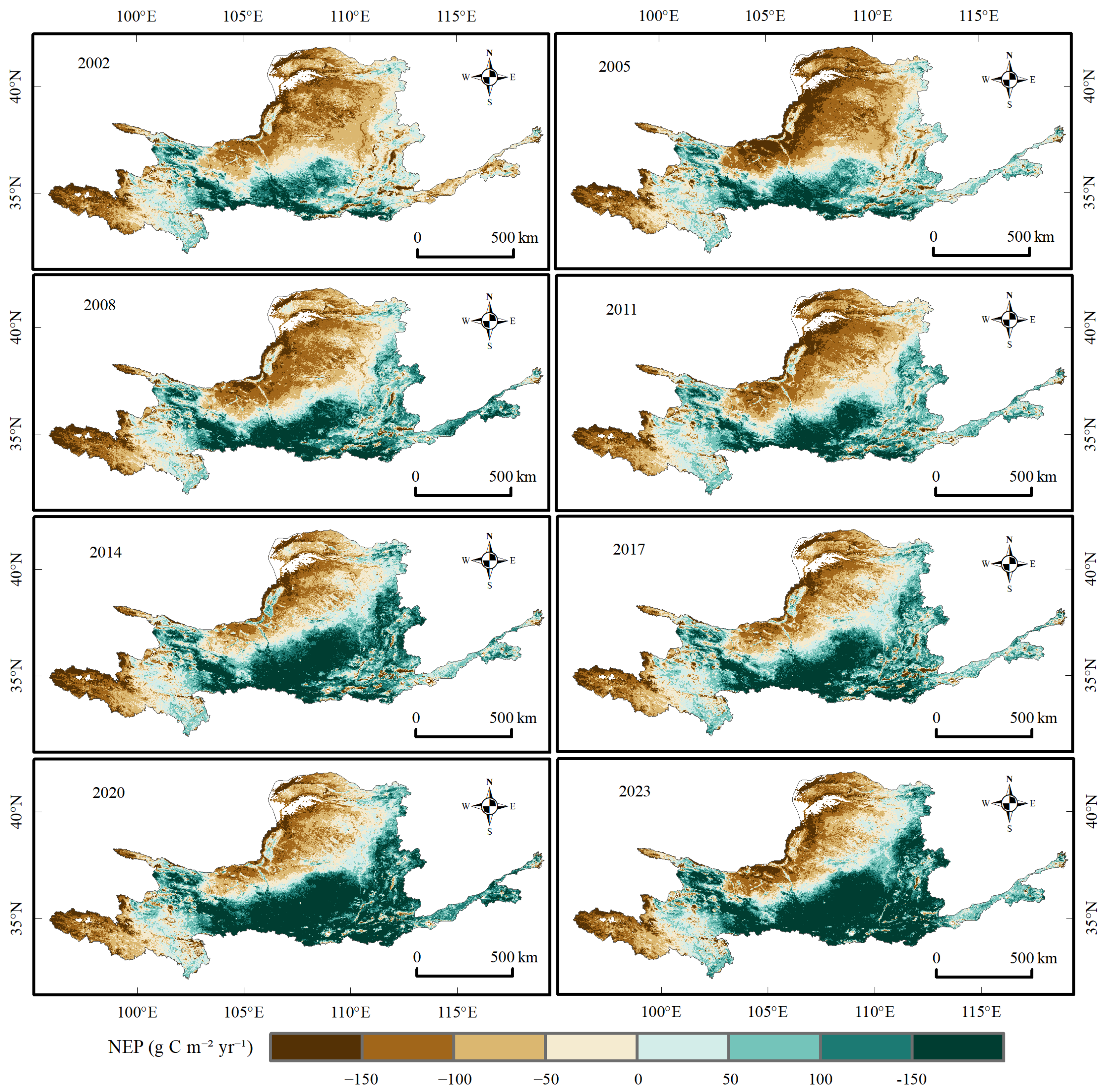
Figure 1 illustrates the spatial evolution of NEP using eight representative years (2002, 2005, 2008, 2011, 2014, 2017, 2020, and 2023). Positive values predominated in the southern, middle, and lower reaches, where carbon-sink areas formed contiguous patches or bands. Negative values predominated in the north and parts of the upper reaches, where carbon-source areas were spatially clustered. The transition zone between sources and sinks was mainly located in the central basin. Comparison across the eight maps shows that the broad spatial configuration remained recognizable, while interannual change was expressed mainly through the intensity and extent of sources and sinks and localized shifts in the transition zone. At the basin scale, NEP followed a clear southeast-to-northwest gradient: humid and relatively warm southern and eastern sectors, together with the middle and lower reaches, formed the main sink belt, whereas the arid and semi-arid northern and upper reaches contained most source patches. The central basin acted as a transition belt in which source–sink boundaries shifted between years. This regional organization is more persistent than the year-to-year change in local intensity, indicating that hydrothermal zonation provides the dominant geographic background for the observed NEP pattern, while local land cover and restoration conditions likely modulate the patch-level differences.

Figure 1. Spatial patterns of NEP in eight representative years (2002, 2005, 2008, 2011, 2014, 2017, 2020, and 2023). Positive NEP denotes a carbon sink and negative NEP denotes a carbon source; units are g C m⁻² yr⁻¹.

The positive mean should therefore be interpreted as a weak model-derived residual under the baseline product and model assumptions rather than as evidence that the basin is a permanently or uniformly stable carbon sink. The fact that the interannual standard deviation is approximately twice the mean, together with the sign reversal under plausible component perturbations, requires the basin-level conclusion to remain conditional on the selected NPP product, Rh conversion, static SOC approximation, and common-mask aggregation.

The corrected linear trends estimated from the same annual series were 4.69 g C m⁻² yr⁻² for NPP, 0.37 g C m⁻² yr⁻² for Rh, and 4.32 g C m⁻² yr⁻² for NEP. The identity is therefore preserved at the annual pixel level and in the area-weighted trend estimates within numerical precision. Trend significance and historical persistence are reported separately.

3.1.2. Interannual Variation and Stage-Specific Transitions in NEP

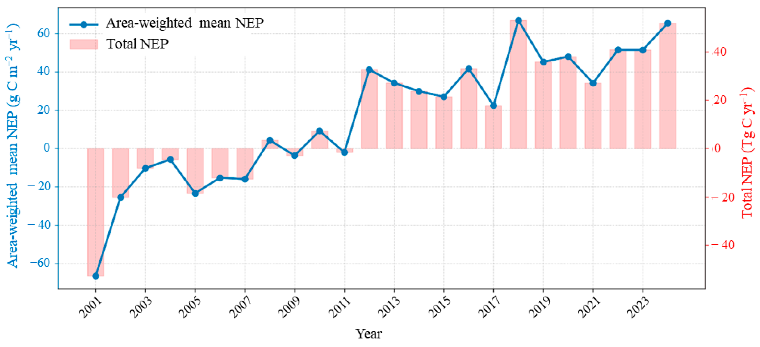
Figure 2 traces the annual trajectories of area-weighted mean NEP (blue line, left axis) and total NEP (pink bars, right axis) from 2001 to 2024. Both series reveal a stage-specific transition from a carbon source to a carbon sink. Area-weighted mean NEP was −66.74 g C m⁻² yr⁻¹ in 2001 and −16.01 g C m⁻² yr⁻¹ in 2007. During 2008–2011, it was 4.25, −3.78, 8.96, and −2.25 g C m⁻² yr⁻¹, respectively. NEP remained positive after 2012, reached 66.83 g C m⁻² yr⁻¹ in 2018, and was 51.44, 51.39, and 65.21 g C m⁻² yr⁻¹ in 2022, 2023, and 2024, respectively. The two series show the same early-2010s transition under the baseline common-mask calculation.

Figure 2. Interannual variation in area-weighted mean NEP (blue line; left axis, g C m⁻² yr⁻¹) and total NEP (pink bars; right axis, Tg C yr⁻¹) in the Yellow River Basin from 2001 to 2024.

Annual total NEP showed the same stage-specific pattern. It was −52.89 Tg C yr⁻¹ in 2001 and −12.69 Tg C yr⁻¹ in 2007. Values for 2008–2011 were 3.37, −3.00, 7.10, and −1.78 Tg C yr⁻¹, respectively. Annual total NEP increased to 32.50 Tg C yr⁻¹ in 2012, reached 52.96 Tg C yr⁻¹ in 2018, and was 51.68 Tg C yr⁻¹ in 2024. Both the area-weighted mean and annual total indicate substantially greater net carbon uptake after 2012 than during the preceding period.

3.1.3. Spatial Variation in NEP Trend Slopes and Significance

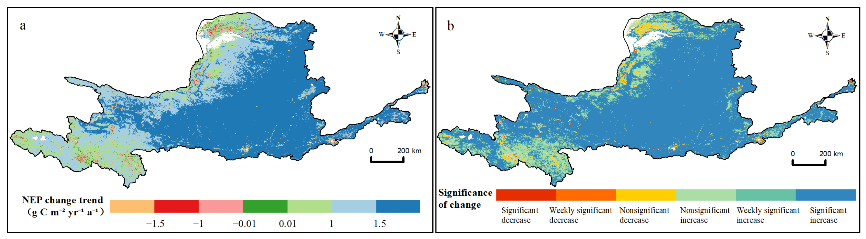
The original local trend-raster audit found significantly increasing trends over 621,860.65 km² (78.0239%). Weakly significant and nonsignificant increases occupied 44,832.84 km² (5.6251%) and 98,217.18 km² (12.3232%), respectively. Undefined trend diagnostics occupied 4652.16 km² (0.5837%) and were retained separately in Table 2. Significant, weakly significant and nonsignificant decreases occupied 3100.38 km² (0.3890%), 1154.00 km² (0.1448%) and 15,030.84 km² (1.8859%), respectively. Near-stable slopes occupied 8164.49 km² (1.0244%). The updated low-memory MK comparison reports all significant p-values regardless of trend direction and therefore is not numerically interchangeable with the directional classes in Table 2.

Table 2. Original local-raster NEP trend classes. Percentages use 797,012.55 km²; undefined diagnostics are retained as a separate row. Slope s is in g C m⁻² yr⁻². The updated low-memory H/MK audit uses a 797,012.56 km² denominator and reports an all-direction p-value comparison separately.

Class	Rule or Diagnostic	Pixels	Area (km2)	Area (%)
Undefined trend	Required slope or p invalid	5783	4652.16	0.5837
Significant decrease	s < −0.1; p ≤ 0.05	3878	3100.38	0.3890
Weakly significant decrease	s < −0.1; 0.05 < p ≤ 0.10	1439	1154.00	0.1448
Nonsignificant decrease	s < −0.1; p > 0.10	18,919	15,030.84	1.8859
Near stable	−0.1 ≤ s ≤ 0.1; any valid p	10,239	8164.49	1.0244
Nonsignificant increase	s > 0.1; p > 0.10	122,543	98,217.18	12.3232
Weakly significant increase	s > 0.1; 0.05 < p ≤ 0.10	55,943	44,832.84	5.6251
Significant increase	s > 0.1; p ≤ 0.05	777,575	621,860.65	78.0239

The maps show that significant increases formed a largely contiguous pattern across the basin, whereas significant or weakly significant decreases were scattered mainly along basin margins and in localized patches (Figure 3). The area statistics in Table 2 quantify this visual contrast: increasing classes dominated, while all decreasing classes together occupied only a small fraction of the analyzed area. We did not attribute the drivers of the declining patches; their causes require further testing using climate, land-use, and ecological-restoration data. Geographically, the increasing classes were concentrated in the southern, middle, and lower reaches and formed a connected belt, whereas declining patches were more common along the northern and peripheral parts of the basin and around local transition zones. The contrast indicates a basin-wide directional tendency superimposed on localized instability rather than a uniform increase everywhere.

Figure 3. Magnitude and significance of pixel-level NEP trends during 2001–2024: (a) trend slope (g C m⁻² yr⁻²) and (b) trend-significance class based on slope direction and Mann–Kendall p value.

3.1.4. Historical Dependence of NEP and Trend Evidence

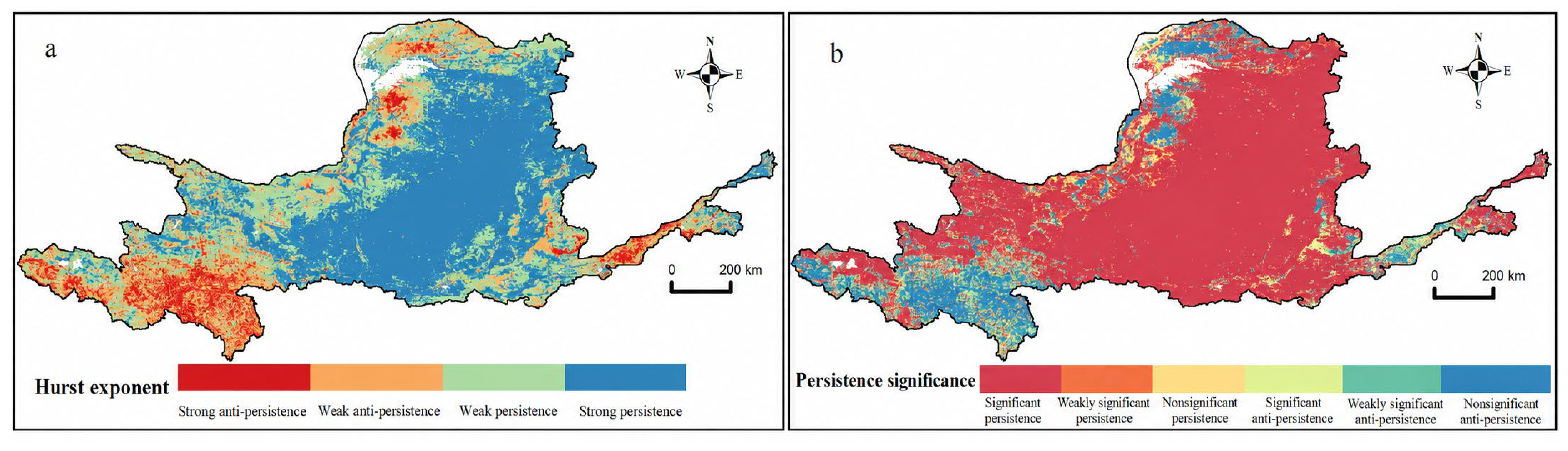
Figure 4 combines two complementary views of historical dependence: the continuous Hurst exponent (Figure 4a) and the categorical overlay of persistence direction and trend evidence (Figure 4b). Areas classified as persistent historical dependence were relatively contiguous, whereas anti-persistent areas were more scattered. The Hurst exponent describes dependence in the 2001–2024 series and does not forecast subsequent direction. The persistent areas broadly followed the main sink belt in the southern and middle-to-lower reaches, while anti-persistent or weakly organized areas were more scattered toward the northern margin and the source–sink transition belt. This spatial contrast links the persistence diagnostic to the basin’s geographic differentiation without treating H as a forecast.

Figure 4. Spatial pattern and significance of NEP persistence during 2001–2024: (a) Hurst exponent and (b) persistence classes obtained by combining Hurst direction with trend significance. Persistence denotes historical statistical dependence rather than a deterministic forecast.

The raw Hurst diagnostic classified 741,200.23 km² (92.9973%) as persistent (H > 0.5), whereas the detrended diagnostic classified 541,598.36 km² (67.9536%) as persistent. In the joint raw-H/raw-MK comparison, persistent areas with significant, weak and nonsignificant trend evidence occupied 625,124.53 km² (78.4335%), 37,859.24 km² (4.7501%) and 78,216.46 km² (9.8137%), respectively. In the detrended-H/TFPW-MK comparison, the corresponding proportions were 56.9366%, 2.8424% and 8.1746%. These are joint descriptive categories rather than significance tests of H (Table 3). The detrending comparison shows that the persistence classification is sensitive to the treatment of the underlying trend and should not be interpreted as a robust forecast of future stability.

Table 3. Local-raster historical dependence crossed with trend evidence. H uses a 0.5 threshold and p refers to the MK trend test, not significance of H. Percentages use the 797,012.56 km² common local mask.

Class	Rule or Diagnostic	Area (km2)	Area (%)
Undefined H or trend evidence	No undefined H or MK p values in the current common-mask audit	0.00	0.0000
Anti-persistent; significant trend	H < 0.5; p ≤ 0.05	2829.81	0.3551
Anti-persistent; weak trend evidence	H < 0.5; 0.05 < p ≤ 0.10	8613.30	1.0807
Anti-persistent; nonsignificant trend	H < 0.5; p > 0.10	44,369.21	5.5669
Boundary; significant trend	H = 0.5; p ≤ 0.05	0.00	0.0000
Boundary; weak trend evidence	H = 0.5; 0.05 < p ≤ 0.10	0.00	0.0000
Boundary; nonsignificant trend	H = 0.5; p > 0.10	0.00	0.0000
Persistent; significant trend	H > 0.5; p ≤ 0.05	625,124.53	78.4335
Persistent; weak trend evidence	H > 0.5; 0.05 < p ≤ 0.10	37,859.24	4.7501
Persistent; nonsignificant trend	H > 0.5; p > 0.10	78,216.46	9.8137

3.1.5. Stability-Risk Zoning of NEP and Sensitivity to Rh

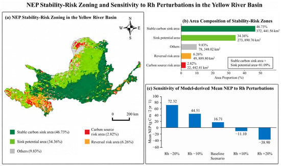
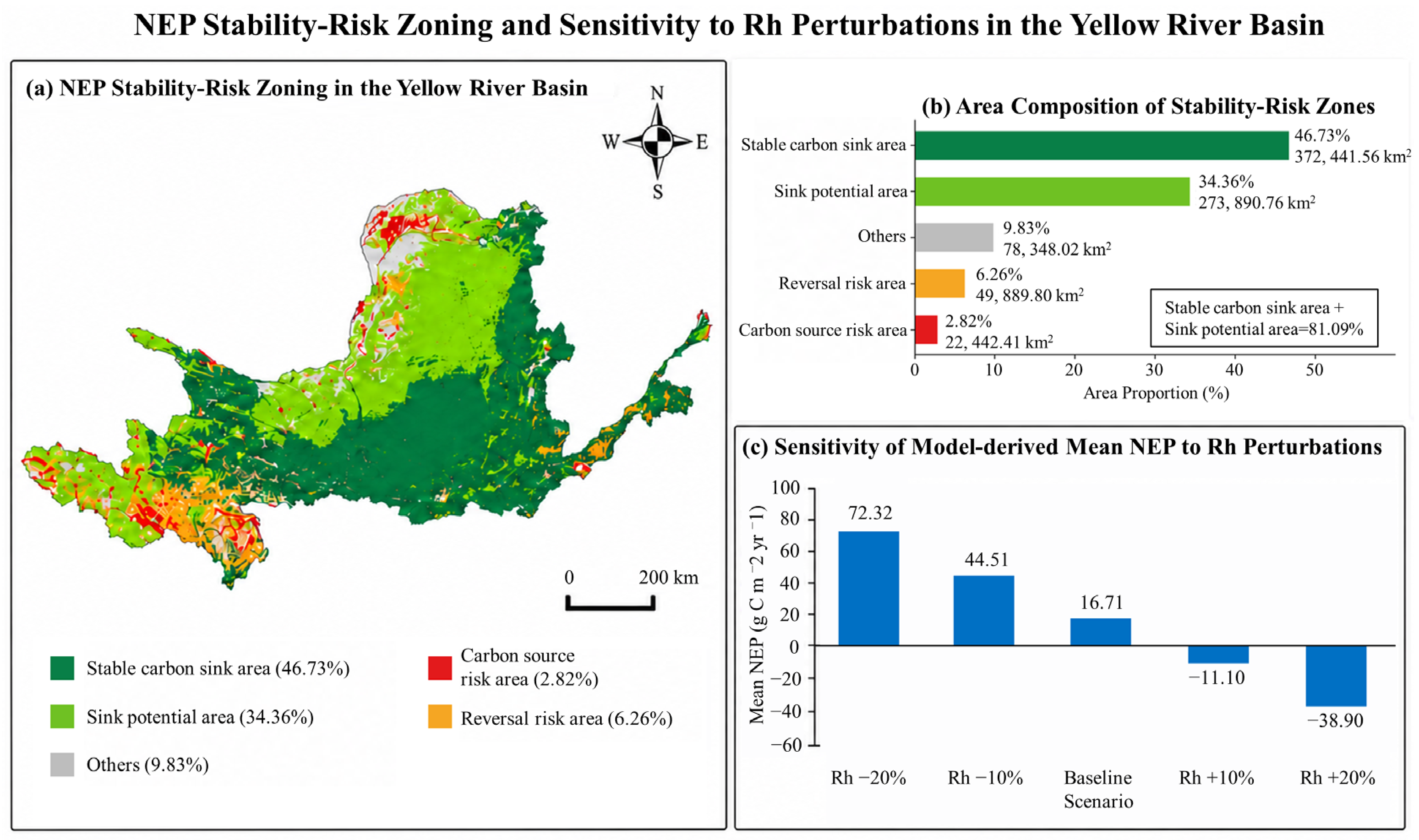
The final risk-rule audit identified stable-sink, sink-potential, carbon-source-risk, reversal-risk, and Other areas of 372,441.56 km² (46.7297%), 273,890.76 km² (34.3647%), 22,442.41 km² (2.8158%), 49,889.80 km² (6.2596%), and 78,348.02 km² (9.8302%), respectively (Table 4). The five categories sum to the 797,012.55–797,012.56 km² local audit area after rounding (Figure 5a and Figure 5b). The explicit rule tree is defined in Section 2.5.

Table 4. Final baseline local risk-rule audit. The ordered classification criteria are explicit in Table 1; areas use the local common-mask denominator and sum to the total after rounding.

Class	Rule or Diagnostic	Pixels	Area (km2)	Area (%)
0 Other	No rule matched or unresolved diagnostic	98,356	78,348.02	9.8302
1 Stable carbon sink	mean > 0; s > 0.1; p ≤ 0.05; H > 0.5	461,796	372,441.56	46.7297
2 Sink potential	mean ≤ 0; s > 0.1; p ≤ 0.10; H > 0.5	346,777	273,890.76	34.3647
3 Carbon source risk	mean < 0; s ≤ 0.1	28,280	22,442.41	2.8158
4 Reversal risk	s > 0.1; H < 0.5; either source or sink	61,110	49,889.80	6.2596

Figure 5. Stability-risk zoning and sensitivity to Rh perturbations: (a) spatial distribution of the five stability-risk zones; (b) final local-mask area and proportion of each zone using approximately 797,012.56 km²; and (c) responses of annual GEE common-mask mean NEP to −20%, −10%, baseline, +10%, and +20% Rh scenarios. The denominators for panels (b) and (c) are therefore distinct.

Carbon-source-risk and reversal-risk areas occupied 22,442.41 km² (2.8158%) and 49,889.80 km² (6.2596%), respectively, whereas Other areas occupied 78,348.02 km² (9.8302%) (Figure 5b). Reversal risk can include pixels that are currently carbon sources, and Other includes pixels whose required diagnostics are undefined; therefore, Other must not be interpreted as a uniformly low-risk category.

The estimated net carbon balance was highly sensitive to heterotrophic respiration and NPP uncertainty. On the annual GEE common valid-pixel mask, the baseline multi-year mean NEP was 16.71 g C m⁻² yr⁻¹. With Rh held at its baseline value, reducing NPP by 10% changed mean NEP to −12.77 g C m⁻² yr⁻¹, whereas increasing NPP by 10% changed it to 46.19 g C m⁻² yr⁻¹. Reducing Rh by 10% increased mean NEP to 44.51 g C m⁻² yr⁻¹, whereas increasing Rh by 10% changed it to −11.10 g C m⁻² yr⁻¹ (Figure 5c). For the local spatial sensitivity audit, the complete NPP–Rh component mask covered 728,286.47 km², equivalent to 91.3770% of the 797,012.56 km² NEP local mask. Across the 15 paired scenarios, the spatial-audit mean NEP ranged from −59.65 to 110.88 g C m⁻² yr⁻¹ (Table 5); the baseline-factor scenario (NPP factor = 1.0, Rh factor = 1.0) yielded 25.61 g C m⁻² yr⁻¹ and a sink area of 54.53% on that component mask. A −10% NPP perturbation with baseline Rh yielded −4.51 g C m⁻² yr⁻¹, whereas a +10% NPP perturbation yielded 55.74 g C m⁻² yr⁻¹; a +10% Rh perturbation with baseline NPP yielded −1.95 g C m⁻² yr⁻¹. The annual GEE values and local spatial-scenario values use different common masks and are therefore not numerically interchangeable. These deterministic results are sensitivity scenarios rather than statistical confidence intervals or probability-based uncertainty bounds.

Table 5. Fifteen paired NPP–Rh spatial sensitivity scenarios on the 728,286.47 km² common component mask.

Scenario	NPP Factor	Rh Factor	Mean NEP (g C m−2 yr−1)	Sink Area (%)	Positive Years
0	0.9	0.8	50.62	63.50	23
1	0.9	0.9	23.05	54.53	18
2	0.9	1.0	−4.51	45.79	13
3	0.9	1.1	−32.08	36.24	2
4	0.9	1.2	−59.65	27.14	0
5	1.0	0.8	80.75	70.46	23
6	1.0	0.9	53.18	62.61	23
7	1.0	1.0	25.61	54.53	18
8	1.0	1.1	−1.95	46.70	13
9	1.0	1.2	−29.52	38.19	6
10	1.1	0.8	110.88	75.88	24
11	1.1	0.9	83.31	69.07	23
12	1.1	1.0	55.74	61.88	23
13	1.1	1.1	28.18	54.53	18
14	1.1	1.2	0.61	47.44	13

3.2. Process Decomposition of NEP: Spatiotemporal Patterns of Productivity and Respiration Fluxes

3.2.1. Spatiotemporal Patterns and Trends of NPP

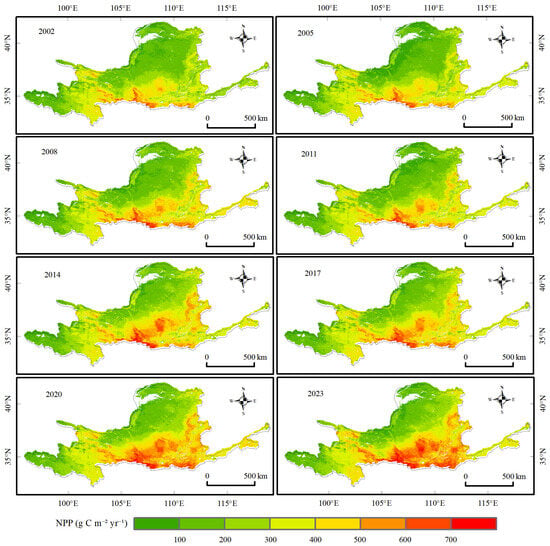
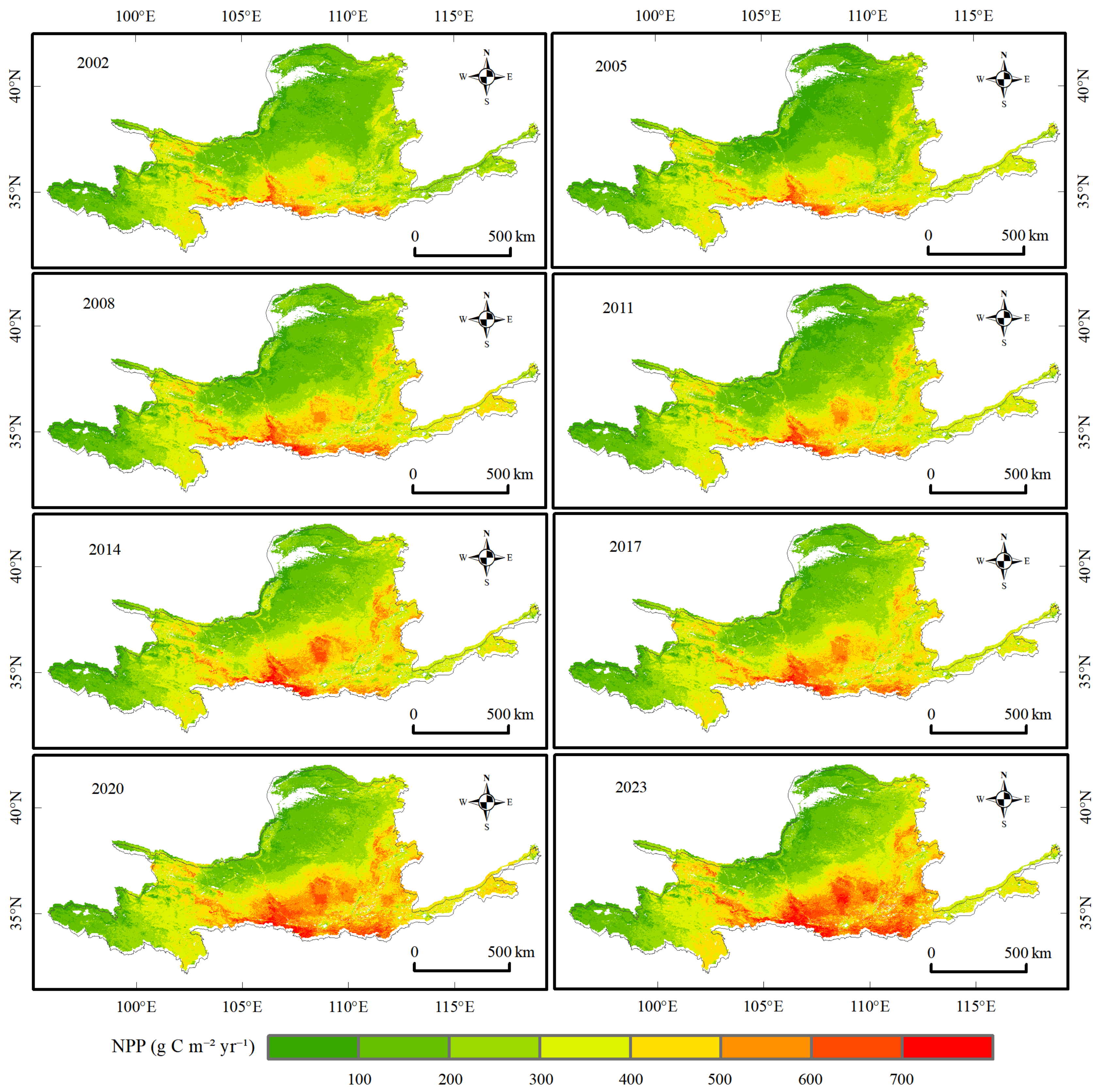
Figure 6 shows NPP for the same eight representative years used in Figure 1, enabling direct comparison between vegetation productivity and net carbon uptake. NPP exhibited a persistent southeast-to-northwest gradient, with higher values along the southern margin and in the middle and lower reaches and lower values in the northern and arid upper reaches. Comparison across panels indicates that the main spatial gradient remained stable, whereas interannual differences were concentrated in the intensity and extent of high-productivity areas.

Figure 6. Spatial patterns of NPP in eight representative years (2002, 2005, 2008, 2011, 2014, 2017, 2020, and 2023); units are g C m⁻² yr⁻¹.

The multi-year mean of annual area-weighted NPP was 294.77 g C m⁻² yr⁻¹, with an interannual standard deviation of 35.69 g C m⁻² yr⁻¹. The annual total averaged 233.60 Tg C yr⁻¹. The minimum occurred in 2001 and the maximum in 2024. During the study period, area-weighted mean NPP increased linearly at 4.69 g C m⁻² yr⁻², while the corresponding annual total trend was calculated from the same common-mask series.

3.2.2. Soil Heterotrophic Respiration Carbon Flux

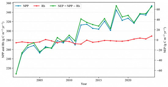
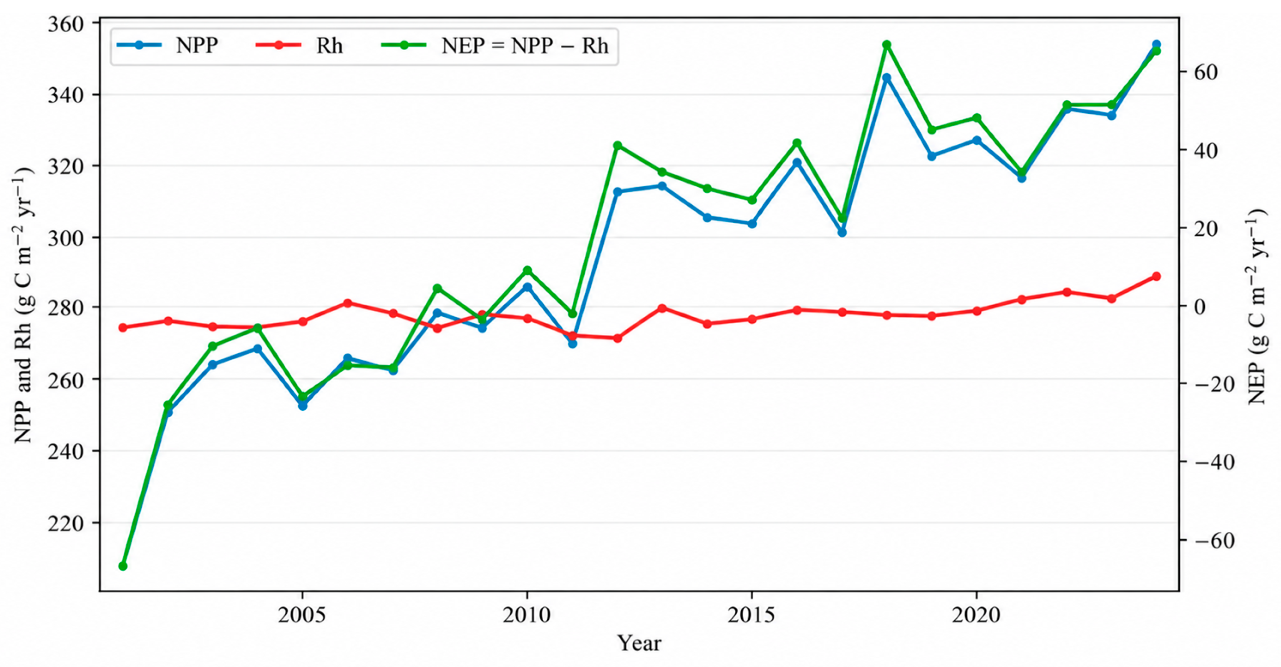
Figure 7 presents the annual common-mask NPP–Rh–NEP accounting series used for the closure check. The corresponding year-by-year carbon-accounting reconciliation is provided in Table S1 in the Supplementary Materials. NPP and Rh are the two component fluxes, and NEP is calculated pixel by pixel as NPP minus Rh before aggregation. Rh remains a model-derived flux obtained from Rs through the fixed empirical conversion and should not be interpreted as a direct observation of microbial respiration.

Figure 7. Annual common-mask NPP, Rh, and NEP series used for carbon-accounting verification from 2001 to 2024; NPP, Rh, and NEP are expressed in g C m⁻² yr⁻¹.

The multi-year mean of annual area-weighted Rh was 278.06 g C m⁻² yr⁻¹, with an interannual standard deviation of 3.93 g C m⁻² yr⁻¹. Mean annual total Rh was 220.36 Tg C yr⁻¹. Rh increased at 0.37 g C m⁻² yr⁻². Because Rh is derived from Rs through a fixed empirical conversion, these values are model estimates rather than direct observations. Area-weighted mean Rh and annual total Rh increased linearly at 0.37 g C m⁻² yr⁻² and 0.290 Tg C yr⁻², respectively; R² was 0.44 for both trends. The much slower increase in Rh than in NPP provides the process-level basis for the strengthening NEP pattern, while the perturbation results in Figure 5c show that the absolute net balance remains sensitive to the estimated respiratory loss.

3.2.3. Spatiotemporal Patterns and Trends of Total Soil Respiration Carbon Flux

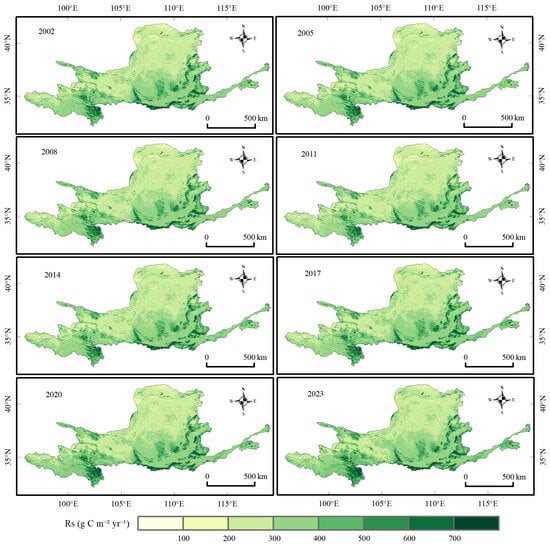
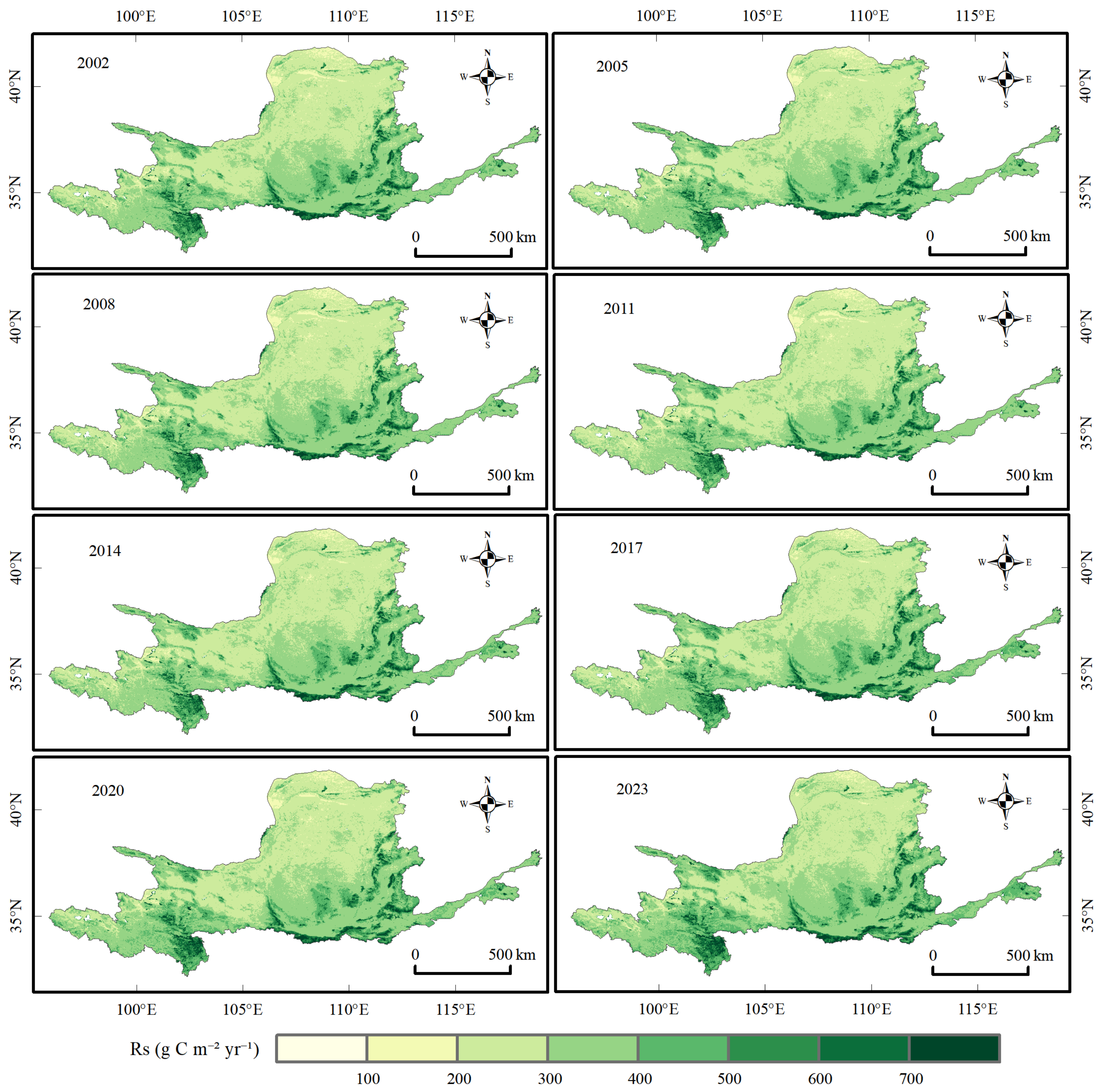
The multi-year mean of annual area-weighted Rs was 349.74 g C m⁻² yr⁻¹, and mean annual total Rs was 277.16 Tg C yr⁻¹. Rs increased at approximately 0.78 g C m⁻² yr⁻² (Figure 8). The Rs series is retained mainly to document the respiration calculation; Rh is a fixed linear transformation of Rs under the baseline conversion. The map sequence indicates higher Rs in the wetter southern and eastern sectors and lower Rs across the drier northern and upper reaches, while the year-to-year pattern remains spatially organized along the basin’s hydrothermal gradient. Because Rh is derived from Rs through a fixed linear conversion, this geographic structure is inherited by the Rh field and contributes directly to the spatial organization of the modeled NEP residual.

Figure 8. Spatial patterns of estimated total soil respiration (Rs) in eight representative years (2002, 2005, 2008, 2011, 2014, 2017, 2020, and 2023); units are g C m⁻² yr⁻¹.

Area-weighted mean Rs and annual total Rs increased linearly at 0.783 g C m⁻² yr⁻² and 0.620 Tg C yr⁻², respectively; R² was 0.44 for both trends. Rs increased slowly during the study period, and its spatial variation was substantially greater than its interannual variation.

4. Discussion

4.1. Comparison with Previous Studies and Consistency of the Results

Similarly, Zhang et al. [31] reported increasing corn NPP and carbon sequestration in the Fen River Basin, which provides a sub-basin productivity benchmark but does not resolve the basin-wide net balance with heterotrophic respiration. Yang et al. [32] developed a multi-objective water–energy–food–carbon optimization model under uncertainty for the Heihe Irrigation Area, emphasizing the trade-offs among irrigation water productivity, carbon outcomes, food production, and resource constraints. That framework is designed for an arid irrigation system and does not provide a pixel-level NEP accounting for the Yellow River Basin. Our study therefore complements these regional and uncertainty-oriented efforts by integrating a common-mask annual carbon accounting identity, explicit spatial diagnostics, and paired NPP–Rh sensitivity scenarios across the entire Yellow River Basin.

Holding SOC constant further means that restoration-related SOC accumulation or depletion is not represented in Rh. The resulting Rh trend may therefore understate or misallocate respiration changes associated with soil-carbon dynamics, and the sign and magnitude of that bias cannot be determined without time-varying SOC observations or an independently calibrated dynamic SOC model.

Absolute NEP estimates, source-area fractions, and transition timing differ among studies because regional net fluxes are sensitive to the selected NPP product, meteorological forcing, soil-respiration model, Rh partitioning scheme, spatial resolution, and study period [12,33,38,39,40]. These methodological differences are not merely technical: when regional NEP is near zero, a small systematic bias in either component can reverse the inferred source–sink status. The directional consistency among studies therefore supports the broad pattern of sink strengthening, whereas disagreement in magnitude underscores the need to report process components and uncertainty alongside the net flux.

4.2. Drivers of Spatial Variation in NEP and Estimation Uncertainty

The southeast-to-northwest decline in precipitation provides a first-order explanation for the basin’s spatial NEP gradient. Water availability constrains canopy development and photosynthesis and can amplify the effects of heat and atmospheric dryness on carbon uptake [10,24,25,40]. In the south and southeast, relatively favorable hydrothermal conditions support higher NPP and NEP. In the arid and semi-arid north, lower and more variable water supply restricts productivity and increases exposure to drought-related sink weakening. Importantly, moisture can affect both sides of the NEP balance: drought suppresses photosynthesis, whereas rewetting and warmer conditions can stimulate decomposition. Thus, similar greening trends may produce different net-carbon outcomes along the basin’s hydrothermal gradient. This mechanism is consistent with our maps, but it remains a hypothesis because the present analysis did not perform formal driver attribution.

Land-use change and ecological restoration may also have contributed to stronger NPP and NEP. Programs such as Grain for Green can increase vegetation biomass and reduce land degradation, but their net-carbon benefits depend on vegetation type, stand age, soil-carbon response, and water availability [21,22,23,26,27,41]. In water-limited landscapes, maximizing vegetation cover may increase evapotranspiration and expose restoration gains to drought stress. The management-relevant question is therefore not whether restoration increases greenness, but whether productivity gains remain larger than respiratory and disturbance losses without exceeding local water-resource carrying capacity. Our results are compatible with a restoration contribution, yet NEP trends alone cannot identify the causal effect or additionality of any individual program.

The Hurst exponent provides additional information on the historical dependence structure of NEP variability. However, because the calculation is based on a relatively short 24-year annual series without multiple-window regression or bootstrap uncertainty, it should not be interpreted as evidence of future ecosystem persistence or resilience. The raw series yielded H > 0.5 over 92.9973% of the common local mask, whereas the proportion decreased to 67.9536% after linear detrending. This comparison indicates that the underlying trend contributes substantially to the apparent persistence pattern. H-based categories are therefore treated as supplementary historical diagnostics rather than independent evidence of ecosystem resilience.

The scenario spread demonstrates that the estimated sink is structurally uncertain. The annual GEE common-mask baseline mean NEP was 16.71 g C m⁻² yr⁻¹; a −10% NPP perturbation with baseline Rh produced −12.77 g C m⁻² yr⁻¹, whereas a +10% NPP perturbation produced 46.19 g C m⁻² yr⁻¹. A +10% Rh perturbation changed the annual mean to −11.10 g C m⁻² yr⁻¹. The local spatial audit, conducted on the 728,286.47 km² common NPP–Rh mask, produced a mean NEP range of −59.65 to 110.88 g C m⁻² yr⁻¹ across 15 scenarios; the baseline-factor scenario had a mean of 25.61 g C m⁻² yr⁻¹ and 54.53% sink area. These spatial-scenario values use a separate component-valid denominator and are not substituted for the annual GEE accounting values. The results show that both NPP and Rh assumptions can change the inferred source–sink interpretation.

4.3. Implications for Basin Management and Future Research

The risk classification translates net-flux patterns into differentiated management priorities [42]. Stable-sink areas should be managed to protect existing vegetation and soil-carbon functions and to reduce disturbance-driven losses. Sink-enhancement-potential areas warrant targeted restoration only where water availability and ecosystem carrying capacity support additional biomass. Reversal-risk areas require early-warning monitoring because a historically positive NEP trend does not ensure persistence under future drought, warming, fire, or land-use pressure. Persistent-source areas should be evaluated for the feasibility and water cost of intervention rather than assigned uniform greening targets. This hierarchy avoids equating greater vegetation cover with a durable carbon sink and is consistent with the place-based, water-constrained approach advocated for the basin [23,43,44].

Three priorities would most improve inference and decision relevance. First, NPP and Rh should be constrained jointly with eddy-covariance, soil-respiration, biomass, and SOC observations, and structural uncertainty should be quantified with alternative products and model ensembles. Second, event-scale processes—including drought, rewetting, freeze–thaw cycles, fire, and land-use transitions—should be resolved because annual aggregation can conceal short-lived but consequential carbon losses. Third, restoration effects should be tested using explicit counterfactual or attribution designs and evaluated within a carbon–water–soil-service framework. Such analyses would distinguish gross greening benefits from additional and durable net carbon sequestration, identify thresholds beyond which restoration becomes water limited, and provide a stronger basis for adaptive management under climate change [7,23,43,44].

5. Conclusions

Using multi-source data for 2001–2024, we estimated Rs with a semi-empirical model, derived Rh using an empirical relationship, and calculated NEP by subtracting Rh from remote-sensing-based NPP. We then analyzed the spatiotemporal variation, process contributions, persistence, and stability risks of NEP in the Yellow River Basin. The main conclusions are as follows:

(1)

The Yellow River Basin showed a weak positive model-derived NEP residual on the common valid-pixel mask. The multi-year mean was 16.71 g C m⁻² yr⁻¹ and the mean annual total was 13.24 Tg C yr⁻¹, with an interannual standard deviation of 33.55 g C m⁻² yr⁻¹. The estimate is conditional on the MODIS NPP product, the semi-empirical Rs model, the empirical Rh conversion, the static SOC approximation, and the common-grid resampling procedure; it should not be treated as a direct measurement of basin carbon sequestration.

(2)

Under the baseline calculation, annual NEP was positive in 2008, 2010, and 2012–2024. Its area-weighted linear trend was 4.32 g C m⁻² yr⁻². This timing is conditional on the product, common mask, and Rh conversion and is not treated as an absolute critical year.

(3)

Rising NPP contributed more strongly than the baseline Rh trend to the modeled NEP increase. NPP increased at 4.69 g C m⁻² yr⁻², whereas Rh increased at 0.37 g C m⁻² yr⁻². Hurst values describe statistical dependence in the 2001–2024 historical series; they do not predict future NEP or prove significant persistence relative to H = 0.5.

(4)

The stability-risk zones are conditional classifications. The final baseline audit identified stable-sink, sink-potential, carbon-source-risk, reversal-risk, and Other areas of 46.7297%, 34.3647%, 2.8158%, 6.2596%, and 9.8302%, respectively. The baseline Rh and NPP results should be interpreted together with the 15-scenario sensitivity range. Stable-sink and enhancement-potential areas are conditional management hypotheses, whereas reversal-risk and source-risk areas identify priorities for monitoring and additional validation. A positive baseline mean alone is insufficient to establish a stable basin-wide carbon sink.

References

- Friedlingstein, P.; O’Sullivan, M.; Jones, M.W.; Andrew, R.M.; Bakker, D.C.E.; Hauck, J.; Landschützer, P.; Le Quéré, C.; Li, H.; Luijkx, I.T.; et al. Global Carbon Budget 2025. Earth Syst. Sci. Data 2026, 18, 3211–3288. [Google Scholar] [CrossRef] [Scilit]
- Friedlingstein, P.; Le Quéré, C.; O’Sullivan, M.; Hauck, J.; Landschützer, P.; Luijkx, I.T.; Li, H.; van der Woude, A.; Schwingshackl, C.; Pongratz, J.; et al. Emerging climate impact on carbon sinks in a consolidated carbon budget. Nature 2026, 649, 98–103. [Google Scholar] [CrossRef] [Scilit] [PubMed]
- Piao, S.; Fang, J.; Ciais, P.; Peylin, P.; Huang, Y.; Sitch, S.; Wang, T. The carbon balance of terrestrial ecosystems in China. Nature 2009, 458, 1009–1013. [Google Scholar] [CrossRef] [Scilit] [PubMed]
- Wang, J.; Feng, L.; Palmer, P.I.; Liu, Y.; Fang, S.; Bösch, H.; O’dell, C.W.; Tang, X.; Yang, D.; Liu, L.; et al. Large Chinese land carbon sink estimated from atmospheric carbon dioxide data. Nature 2020, 586, 720–723. [Google Scholar] [CrossRef] [Scilit] [PubMed]
- Zhu, Y.; Xia, X.; Canadell, J.G.; Piao, S.; Lu, X.; Mishra, U.; Wang, X.; Yuan, W.; Qin, Z. China’s carbon sinks from land-use change underestimated. Nat. Clim. Change 2025, 15, 428–435. [Google Scholar] [CrossRef] [Scilit]
- Song, J.; Wan, S.; Piao, S.; Xia, J.; Ning, Y.; Zheng, M.; Hui, D.; Ru, J.; Han, J.; Feng, J.; et al. Global change and China’s terrestrial carbon sink: A quantitative review of 30 years’ ecosystem manipulative experiments. Ecol. Monogr. 2025, 95, e70005. [Google Scholar] [CrossRef] [Scilit]
- United Nations. Transforming Our World: The 2030 Agenda for Sustainable Development; United Nations: New York, NY, USA, 2015. [Google Scholar]
- Poulter, B.; Frank, D.; Ciais, P.; Myneni, R.B.; Andela, N.; Bi, J.; Broquet, G.; Canadell, J.G.; Chevallier, F.; Liu, Y.Y.; et al. Contribution of semi-arid ecosystems to interannual variability of the global carbon cycle. Nature 2014, 509, 600–603. [Google Scholar] [CrossRef] [Scilit] [PubMed]
- Humphrey, V.; Berg, A.M.; Ciais, P.; Gentine, P.; Jung, M.; Reichstein, M.; Seneviratne, S.I.; Frankenberg, C. Soil moisture–atmosphere feedback dominates land carbon uptake variability. Nature 2021, 592, 65–69. [Google Scholar] [CrossRef] [Scilit] [PubMed]
- Wang, F.; Zhang, Z.; Du, M.; Lu, J.; Chen, X. Drought amplifies the suppressive effect of afforestation on net primary productivity in semi-arid ecosystems: A case study of the Yellow River Basin. Remote Sens. 2025, 17, 2100. [Google Scholar] [CrossRef] [Scilit]
- Zhao, M.; Running, S.W. Drought-induced reduction in global terrestrial net primary production from 2000 through 2009. Science 2010, 329, 940–943. [Google Scholar] [CrossRef] [Scilit] [PubMed]
- Ji, S.; Ren, S.; Fang, L.; Chen, J.; Wang, G.; Wang, Q. Improved CASA-based net ecosystem productivity estimation in China by incorporating developmental factors into autumn phenology model. Remote Sens. 2025, 17, 487. [Google Scholar] [CrossRef] [Scilit]
- Hashimoto, S.; Ito, A.; Nishina, K. Harmonized global soil carbon and respiration datasets with derived turnover time and temperature sensitivity. Sci. Data 2025, 12, 2005. [Google Scholar] [CrossRef] [Scilit] [PubMed]
- Yan, Y.; Wohlfahrt, G.; Huang, N.; Cao, M.; Wang, X. Climate and vegetation-driven increase of soil heterotrophic and autotrophic respiration in China’s subtropical forests over 2000–2020. Glob. Biogeochem. Cycles 2025, 39, e2024GB008363. [Google Scholar] [CrossRef] [Scilit]
- Bond-Lamberty, B.; Wang, C.K.; Gower, S.T. A global relationship between the heterotrophic and autotrophic components of soil respiration? Glob. Change Biol. 2004, 10, 1756–1766. [Google Scholar] [CrossRef] [Scilit]
- Yu, G.R.; Zheng, Z.M.; Wang, Q.F.; Fu, Y.; Zhuang, J.; Sun, X.; Wang, Y. Spatiotemporal pattern of soil respiration of terrestrial ecosystems in China: The development of a geostatistical model and its simulation. Environ. Sci. Technol. 2010, 44, 6074–6080. [Google Scholar] [CrossRef] [Scilit] [PubMed]
- Zheng, Z.M.; Yu, G.R.; Sun, X.M.; Li, S.-G.; Wang, Y.-S.; Wang, Y.-H.; Fu, Y.-L.; Wang, Q.-F. Spatio-temporal variability of soil respiration of forest ecosystems in China: Influencing factors and evaluation model. Environ. Manag. 2010, 46, 633–642. [Google Scholar] [CrossRef] [Scilit] [PubMed]
- Han, L.; Yu, G.R.; Chen, Z.; Zhu, X.; Zhang, W.; Wang, T.; Xu, L.; Chen, S.; Liu, S.; Wang, H.; et al. Spatiotemporal pattern of ecosystem respiration in China estimated by integration of machine learning with ecological understanding. Glob. Biogeochem. Cycles 2022, 36, e2022GB007439. [Google Scholar] [CrossRef] [Scilit]
- Yu, Z.; Ciais, P.; Piao, S.; Houghton, R.A.; Lu, C.; Tian, H.; Agathokleous, E.; Kattel, G.R.; Sitch, S.; Goll, D.; et al. Forest expansion dominates China’s land carbon sink since 1980. Nat. Commun. 2022, 13, 5374. [Google Scholar] [CrossRef] [Scilit] [PubMed]
- Yue, C.; Xu, M.; Ciais, P.; Tao, S.; Shen, H.; Chang, J.; Li, W.; Deng, L.; He, J.; Leng, Y.; et al. Contributions of ecological restoration policies to China’s land carbon balance. Nat. Commun. 2024, 15, 9708. [Google Scholar] [CrossRef] [Scilit] [PubMed]
- Deng, L.; Shangguan, Z.P.; Sweeney, S. ‘Grain for Green’ driven land use change and carbon sequestration on the Loess Plateau, China. Sci. Rep. 2014, 4, 7039. [Google Scholar] [CrossRef] [Scilit] [PubMed]
- Ma, Y.Q.; Li, J.H.; Cao, W.; Huang, L. Grain for Green Program to Grassland Might Lead to Carbon Sink Leakage in the Loess Plateau. Earth’s Future 2025, 13, e2024EF005261. [Google Scholar] [CrossRef] [Scilit]
- Feng, X.M.; Fu, B.J.; Piao, S.L.; Wang, S.; Ciais, P.; Zeng, Z.; Lü, Y.; Zeng, Y.; Li, Y.; Jiang, X.; et al. Revegetation in China’s Loess Plateau is approaching sustainable water resource limits. Nat. Clim. Change 2016, 6, 1019–1022. [Google Scholar] [CrossRef] [Scilit]
- Sun, R.; Liu, C.M.; Zhu, Q.J. Relationship between vegetation-cover dynamics and precipitation in the Yellow River Basin. Acta Geogr. Sin. 2001, 56, 667–672. (In Chinese) [Google Scholar]
- Tian, Z.H.; Ren, Z.G.; Wei, H.T. Driving mechanisms of spatiotemporal vegetation evolution in the Yellow River Basin from 2000 to 2020. Environ. Sci. 2022, 43, 743–751. (In Chinese) [Google Scholar] [CrossRef] [Scilit] [PubMed]
- Ren, Z.G.; Tian, Z.H.; Wei, H.T.; Liu, Y.; Yu, Y. Spatiotemporal evolution and driving mechanisms of vegetation in the Yellow River Basin, China during 2000–2020. Ecol. Indic. 2022, 138, 108832. [Google Scholar] [CrossRef] [Scilit]
- Liu, C.X.; Zhang, X.D.; Wang, T.; Chen, G.; Zhu, K.; Wang, Q.; Wang, J. Detection of vegetation coverage changes in the Yellow River Basin from 2003 to 2020. Ecol. Indic. 2022, 138, 108818. [Google Scholar] [CrossRef] [Scilit]
- Tian, K.; Liu, X.; Zhang, B.; Wang, Z.; Xu, G.; Chang, K.; Xu, P.; Han, B. Analysis of spatiotemporal evolution and influencing factors of vegetation net primary productivity in the Yellow River Basin from 2000 to 2022. Sustainability 2024, 16, 381. [Google Scholar] [CrossRef] [Scilit]
- Hou, X.; Zhang, B.; He, Q.Q.; Shao, Z.-L.; Yu, H.; Zhang, X.-Y. Spatial–temporal variations in the climate, net ecosystem productivity, and efficiency of water and carbon use in the middle reaches of the Yellow River. Remote Sens. 2024, 16, 3312. [Google Scholar] [CrossRef] [Scilit]
- Chen, Y.; Xu, Y.; Chen, T.; Zhang, F.; Zhu, S. Exploring the spatiotemporal dynamics and driving factors of net ecosystem productivity in China from 1982 to 2020. Remote Sens. 2024, 16, 60. [Google Scholar] [CrossRef] [Scilit]
- Zhang, Z.; Huo, L.; Su, Y.; Shen, H.; Yang, G. Estimation of Corn Net Primary Productivity and Carbon Sequestration Based on the CASA Model: A Case Study of the Fen River Basin. Sustainability 2024, 16, 2942. [Google Scholar] [CrossRef] [Scilit]
- Yang, Z.; Li, L.; Su, Y.; Huo, L.; Yang, G. Multi-Objective Collaborative Optimization Model and Application of the Water-Energy-Food-Carbon Nexus Under Uncertainty: A Case Study of the Heihe Irrigation Area. Water 2026, 18, 841. [Google Scholar] [CrossRef] [Scilit]
- Chuai, X.; Qi, X.; Zhang, X.; Li, J.; Yuan, Y.; Guo, X.; Huang, X.; Park, S.; Zhao, R.; Xie, X.; et al. Land degradation monitoring using terrestrial ecosystem carbon sinks/sources and their response to climate change in China. Land Degrad. Dev. 2018, 29, 3489–3502. [Google Scholar] [CrossRef] [Scilit]
- Mann, H.B. Nonparametric tests against trend. Econometrica 1945, 13, 245–259. [Google Scholar] [CrossRef] [Scilit]
- Sen, P.K. Estimates of the regression coefficient based on Kendall’s tau. J. Am. Stat. Assoc. 1968, 63, 1379–1389. [Google Scholar] [CrossRef]
- Kendall, M.G. Rank Correlation Methods; Charles Griffin: London, UK, 1975. [Google Scholar]
- Hurst, H.E. Long-term storage capacity of reservoirs. Trans. Am. Soc. Civ. Eng. 1951, 116, 770–799. [Google Scholar] [CrossRef] [Scilit]
- Cao, Y.; Sun, Y.L.; Jiang, Y.Q.; Wan, J. Spatiotemporal differentiation and driving factors of net ecosystem productivity in the Yellow River Basin. Ecol. Environ. Sci. 2022, 31, 2101–2110. (In Chinese) [Google Scholar]
- Zhang, K.; Zhu, C.; Ma, X.; Zhang, X.; Yang, D.; Shao, Y. Spatiotemporal variation characteristics and dynamic persistence analysis of carbon sources/sinks in the Yellow River Basin. Remote Sens. 2023, 15, 323. [Google Scholar] [CrossRef] [Scilit]
- Ma, C.; Zhang, C.; Luo, Z.; Ji, L. Hydroclimatic thresholds shape the long-term persistence of net ecosystem productivity in the Yellow River Basin (2001–2024). Earth Syst. Environ. 2026, 10, 11069–11088. [Google Scholar] [CrossRef] [Scilit]
- Yin, R.S.; Yin, G.P. China’s primary programs of terrestrial ecosystem restoration: Initiation, implementation, and challenges. Environ. Manag. 2010, 45, 429–441. [Google Scholar] [CrossRef] [Scilit] [PubMed]
- Chen, Y.P.; Fu, B.J.; Zhao, Y.; Wang, K.-B.; Zhao, M.M.; Ma, J.-F.; Wu, J.-H.; Xu, C.; Liu, W.-G.; Wang, H. Sustainable development in the Yellow River Basin: Issues and strategies. J. Clean. Prod. 2020, 263, 121223. [Google Scholar] [CrossRef] [Scilit]
- CPC Central Committee and State Council. Outline of the Plan for Ecological Protection and High-Quality Development of the Yellow River Basin [EB/OL]. 2021. Available online: https://www.mee.gov.cn/zcwj/zyygwj/202110/t20211009_955779.shtml (accessed on 26 August 2026). (In Chinese)
- Standing Committee of the National People’s Congress. Yellow River Protection Law of the People’s Republic of China; Standing Committee of the National People’s Congress: Beijing, China, 2022. (In Chinese)
Disclaimer/Publisher’s Note: The statements, opinions and data contained in all publications are solely those of the individual author(s) and contributor(s) and not of MDPI and/or the editor(s). MDPI and/or the editor(s) disclaim responsibility for any injury to people or property resulting from any ideas, methods, instructions or products referred to in the content. |
© 2026 by the authors. Licensee MDPI, Basel, Switzerland. This article is an open access article distributed under the terms and conditions of the Creative Commons Attribution (CC BY) license.