


Abstract
Coordinating digitalization with green development is increasingly central to urban sustainability, yet average CCD scores alone obscure distributional dynamics, regional inequality, spatial dependence, and local heterogeneity. Using 1296 city–year observations for 108 cities in the Yangtze River Economic Belt (YREB) from 2012 to 2023, we construct digitalization (DIG), green-development (GRE), and coupling coordination degree (CCD) indices and combine kernel density estimation, Dagum Gini decomposition, Global Moran’s I, and local regression. Model selection explicitly compares pooled OLS, a spatial-only GWR-type benchmark, temporal weighted regression (TWR), and geographically and temporally weighted regression (GTWR). Mean CCD increased from 0.3622 to 0.5747, while the separately reported coupling degree (C) rose from 0.5312 to 0.7745. The CCD distribution shifted rightward, with dispersion reaching its sample-period minimum around 2018 and widening thereafter. The overall Gini fell from 0.0873 to 0.0693, while the net between-region contribution rose from 37.68% to 49.90%. CCD remained positively spatially autocorrelated. GTWR yielded the lowest ordinary LOOCV RMSE, the lowest AICc under the stability screen, and the weakest residual spatial dependence, while blocked predictive sensitivity checks revealed task-specific trade-offs. Local GTWR surfaces were most consistently positive for economic development and industrial upgrading, but TWFE attenuated these within-city coefficients, reinforcing a non-causal interpretation.
1. Introduction
Digitalization and the green transition are jointly reshaping urban production, resource allocation, and public governance and are increasingly discussed as a “twin transition” in the international literature [1,2,3,4]. Empirical studies in China link digital-economy development to entrepreneurship and high-quality growth [5], urban green development [6], green total factor productivity [7], urban sustainable development [8], and broader green-economy outcomes [9]. At the same time, ICT networks, data centers, and end-user devices create direct energy demand and life-cycle emissions, and efficiency gains may be partly offset by rebound effects [10,11,12]. Digitalization and green development should therefore be viewed as interacting transition processes rather than as independent trajectories. Measuring their coordination and identifying its regional variation have consequently become important questions in urban sustainability research.
Studies of Chinese cities have increasingly adopted an analytical sequence that combines composite-index construction, coupling-coordination measurement, spatial inequality, and associated-factor analysis. She et al. [13] examined 284 cities using coupling coordination, Dagum Gini decomposition, spatial convergence, and Markov transitions; Zhong et al. [14] investigated digital-economy and green-innovation coupling in Chinese urban agglomerations; and Yu et al. [15] integrated CCD, exploratory spatial data analysis, Dagum Gini decomposition, and geographical detectors to study digital infrastructure and inclusive green growth in the YREB. Recent work has continued to extend digital-economy, green-transition, and multidimensional coordination frameworks [16,17,18,19]. These studies establish the usefulness of CCD for summarizing joint system development, but several distributional and local questions remain insufficiently resolved.
First, annual means and maps for selected years indicate changes in average levels but cannot show whether the city distribution shifts as a whole, narrows, polarizes, or develops a long upper tail. Kernel density estimation (KDE) can reveal changes in distributional location, concentration, dispersion, and tail behavior without imposing a parametric distribution. Second, regional inequality requires more than a single overall dispersion statistic: the contribution of within-region differences, net between-region differences, and distributional overlap may evolve differently. Dagum Gini decomposition provides a direct way to separate these components [20]. Third, digital–green coordination is spatially dependent and potentially nonstationary over both space and time. The association of the same economic, industrial, or innovation factor with CCD may differ across cities and years, which a single global coefficient cannot represent. Global Moran’s I and geographically and temporally weighted regression (GTWR) provide complementary diagnostics of these patterns [21,22,23].
Against this background, this study uses a balanced panel of 108 prefecture-level-and-above cities in the YREB from 2012 to 2023 and constructs digitalization (DIG), green-development (GRE), and coupling coordination degree (CCD) indices. It addresses three research questions. RQ1 asks how digitalization, green development, the CCD-based joint-development measure, and the balance between the two subsystems evolved during the sample period and whether the city distribution exhibits compression, renewed dispersion, polarization, or changing tail behavior. RQ2 asks how the sources of regional inequality and the spatial clustering of CCD changed over time. RQ3 asks whether the local associations of economic development, industrial upgrading, green innovation, human capital, environmental regulation, and openness with CCD vary materially across space and time.
The contribution is primarily substantive: the study distinguishes sustained improvement in the mean CCD-based joint-development measure from changes in dispersion and from changes in the composition of the inequality that remains. In particular, it shows how a rising mean CCD can coexist with renewed cross-city dispersion after the sample-period minimum around 2018 and with an increasing net between-region share. Methodologically, a multiscale diagnostic design links distributional, regional, spatial, and local evidence within one city-level framework centered on CCD, with C reported separately as the balance diagnostic. Relative to She et al.’s [13], which emphasizes convergence and transition dynamics across a broad Chinese-city sample, and Yu et al.’s [15], which combines CCD, exploratory spatial analysis, Dagum decomposition, and geographical detectors for digital infrastructure and inclusive green growth, three features extend this literature. First, KDE and Dagum decomposition jointly distinguish mean improvement from distributional change and from the sources of regional inequality. Second, global, spatial-only, temporal-only, and joint spatiotemporal regressions are estimated on the same observations and covariates, so the use of GTWR is supported by comparative model evidence rather than assumed. Third, the local results are subjected to stability screening, blocked predictive sensitivity checks, panel fixed-effects benchmarks, imputation sensitivity, and alternative measurement checks. The 108-city, 12-year panel also permits consistent comparisons across the upper-, middle-, and lower-reach groups.
2. Literature Review and Analytical Framework
2.1. Interactions Between Digitalization and Green Development
Digital technologies can affect green development through information, allocation, transaction-cost, and innovation channels. City-level studies find that digital-economy development can reduce environmental pollution [24], improve broader urban sustainable-development performance [25], and raise green total factor productivity partly through industrial upgrading [26]. Digital-finance research reports positive associations with green technology innovation [27], green-development efficiency [28,29,30], and the enthusiasm and quality of corporate green innovation [31]; related spatial evidence also links digital finance to broader green-development outcomes [32]. City-level evidence further shows that the digital economy can promote green innovation [33]. These channels can improve monitoring, matching, financing, and process optimization, but they do not imply an automatic environmental dividend. A Jevons-type rebound mechanism can arise when efficiency improvements lower the effective cost of data processing, digital services, or technology use and thereby expand activity. At the same time, communication networks, cloud and computing infrastructure, end-user devices, hardware turnover, and the electricity mix create direct and life-cycle energy and emissions burdens [10,11,12]. The net digital–green relationship is therefore theoretically ambiguous and is better understood as conditional complementarity shaped by scale, composition, and rebound effects.
Regional conditions shape whether potential complementarities outweigh these countervailing pressures. The international twin-transition literature emphasizes territorial capabilities, policy differences, and the regional embeddedness of digital and green innovation [1,2], while ICT-energy research shows that efficiency gains can be partly offset by rebound and life-cycle effects [10,11,12]. Evidence from China links industrial upgrading to greener productivity at prefecture-level and YREB scales [34,35]. Green technology innovation can affect carbon emissions nonlinearly, with human capital conditioning the relationship [36], while human-capital studies connect educational and innovative capabilities to green technology innovation and green-growth convergence [37,38]. These mechanisms imply that improvement in average digital–green performance can coexist with substantial differences in pace, balance, and local correlates across cities and reach groups.
2.2. Coordination Measurement, Distributional Dynamics, and Regional Inequality
Coupling-coordination models have been widely used to assess relationships between the digital economy and green development, digital infrastructure and inclusive green growth, and other interacting urban systems [13,14,15,16,17,18]. Their appeal is that they provide a compact summary of the joint state of two subsystems. The interpretation of the conventional coupling coordination degree (CCD), however, depends on the exact algebraic specification. Under the equal subsystem weights used in this study, the conventional CCD formula simplifies to a symmetric function of the DIG×GRE product; consequently, CCD does not independently distinguish subsystem balance when two observations have the same product. We therefore use digital–green coordination as the broader analytical concept, interpret CCD specifically as a symmetric joint-development summary, and report the coupling term C separately as the direct diagnostic of subsystem balance. This distinction preserves comparability with the existing CCD literature while avoiding the stronger claim that CCD itself contains an additional, independent imbalance penalty. KDE then complements the joint-development measure by revealing shifts in location, peak shape, dispersion, and tail behavior that annual means and static maps cannot show.
Studies of regional inequality commonly use the Gini coefficient, Theil index, or convergence models. Dagum Gini decomposition separates overall inequality into within-region inequality, net between-region inequality, and transvariation, thereby identifying the role of distributional overlap [20]. For the YREB, the upper, middle, and lower reaches differ in industrial structure, urban hierarchy, digital infrastructure, and environmental governance capacity. An overall Gini alone therefore cannot establish whether disparities arise mainly within reaches, between reaches, or from overlap among their distributions. Transvariation is interpreted here as distributional overlap rather than as evidence of a geographic boundary-city effect. Combining KDE and Dagum decomposition makes it possible to examine both how the city distribution moves and where the remaining inequality originates.
2.3. Spatial Dependence, Associated Factors, and the Analytical Framework
Digital infrastructure, innovation networks, production chains, labor markets, and environmental governance extend across administrative boundaries, making spatial clustering of digital–green outcomes plausible. Global Moran’s I provides a direct diagnostic of overall spatial autocorrelation [21]. The six GTWR covariates are included because each captures a distinct structural condition that can shape joint digital–green development. Economic development (ECON) can relax fiscal, infrastructure, and technology-adoption constraints and strengthen environmental service capacity, but scale expansion can simultaneously raise energy and material demand. Industrial upgrading (IND) can shift activity toward services and advanced manufacturing and facilitate adoption of digitally enabled cleaner production, while the persistence of heavy-industry legacies can weaken this relationship [34,35]. Green innovation (GINN) can improve energy efficiency, pollution control, and low-carbon production, although commercialization and absorptive capacity determine whether inventions translate into urban environmental performance [36].
Human capital (HUM) can strengthen absorptive capacity and the operation of digital and green technologies, but highly skilled activity can also be concentrated in energy-intensive digital and advanced-service sectors, so a uniformly positive local association is not assumed [37,38]. Environmental regulation (ER) can induce cleaner innovation and technological redirection through Porter-type and directed-technical-change mechanisms, yet compliance costs, enforcement intensity, and industrial relocation can produce nonlinear or context-dependent responses [39,40,41]. Openness (OPEN), proxied by actual utilized FDI relative to GDP, can transmit capital, management practices, cleaner technologies, and international standards, but its environmental consequences also depend on the scale and composition of investment; recent Chinese city evidence shows that FDI–green innovation relationships vary with local institutional and human-capital conditions [42]. These competing channels motivate a heterogeneity framework rather than directional causal hypotheses.
Accordingly, the empirical framework has five layers: (1) construct DIG and GRE, summarize symmetric joint development with CCD, and assess subsystem balance separately with the coupling term C; (2) use KDE to examine shifts and changes in dispersion in the CCD distribution; (3) use Dagum Gini decomposition to identify the magnitude and sources of regional inequality; (4) use Global Moran’s I to test spatial clustering under baseline and alternative weight matrices; and (5) use GTWR to examine spatially and temporally varying conditional associations for the six structural covariates. Throughout the study, GTWR coefficients are interpreted as local conditional associations rather than intervention effects or causal spillovers.
3. Materials and Methods
3.1. Study Area, Data, and Indicator System
The study uses a harmonized 108-city analytical panel covering 2012–2023, yielding 1296 city–year observations. The broader YREB prefecture-level-and-above administrative universe contains 126 units under the harmonized contemporary definition. The analytical universe retained here consists of the two municipalities and 106 prefecture-level cities (85.7% of the broader administrative universe). Eighteen units are outside the balanced panel: 16 autonomous prefectures, for which fully comparable city-level statistical series are not consistently available, plus Bijie and Tongren, whose administrative reclassification around the start of the study period complicates longitudinal harmonization in the underlying city-statistical sources. Sixteen of these 18 exclusions fall in the upper-reach group and two in the middle group; none are in the lower group. The resulting 108-city convention is consistent with longitudinal YREB city studies [18], but all substantive reach comparisons are interpreted as applying to this harmonized city-type analytical universe rather than to every prefecture-level administrative unit in the YREB. The fixed sample contains 31 upper-reach, 36 middle-reach, and 41 lower-reach cities. The upper reach comprises Yunnan, Sichuan, Guizhou, and Chongqing; the middle reach comprises Jiangxi, Hubei, and Hunan; and the lower reach comprises Shanghai, Jiangsu, Zhejiang, and Anhui. This is an administrative comparison grouping rather than a hydrological segmentation; the city crosswalk and full analytical list are available from the corresponding author upon reasonable request. The indicator system contains eight digitalization and eleven green-development indicators. Digital-finance data draw on the Peking University Digital Financial Inclusion Index [43]. Digital-infrastructure attention is measured from municipal government work reports using a predefined new-digital-infrastructure keyword dictionary; the keyword domain is anchored in the new-digital-infrastructure concept discussed by Chao et al. [44]. Digital patents are classified using the CNIPA Key Digital Technology Patent Classification System (2023; IPC 2022 reference), with overlapping assignments deduplicated. Patent grants rather than applications are used in DIG to emphasize realized, substantively examined digital inventive output, whereas GINN uses applications as a contemporaneous innovation-activity covariate. AI-related enterprise density is constructed from enterprise-registration records using business-scope keywords plus industry-code cross-validation and is interpreted as a broad AI-related digital-ecosystem proxy rather than a census of active AI-specialist firms. The GRE system explicitly includes electricity-consumption intensity as a resource-efficiency/energy-intensity indicator, alongside water, emissions, environmental quality, green-space, and treatment indicators. Carbon emissions are based on European Commission JRC EDGAR_2024_GHG annual grids aggregated to fixed city boundaries, and PM2.5 is based on the CHAP ChinaHighPM2.5 1 km annual product series. Variable-level observed/imputed counts are reported in Appendix A Table A4.
After data integration, the 25 core variables form a balanced panel of 108 cities over 2012–2023. Missing values were first addressed through within-city temporal interpolation and then through inverse-distance weighting (IDW; power = 2) using the five nearest valid donor cities, with priority given to the same province and river reach. Overall, 1260 of 32,400 observations (3.89%) were imputed, predominantly using IDW. Missingness was concentrated in digital patents and AI-related firms, park green space, GINN, HUM, and digital-infrastructure attention; the remaining 19 variables were complete. Original observations and imputation flags were retained, and sensitivity checks are reported in Section 4.5 and Appendix A Table A3.
For GTWR estimation, the six covariates were winsorized at the pooled 1st and 99th percentiles and globally standardized, while CCD remained on its original scale. Table 1, Table 2 and Table 3 present the indicator system and entropy weights, covariate definitions, and descriptive statistics in original units, respectively.
Table 1.
Indicator system for digitalization and green development.
Table 2.
Definitions of GTWR covariates.
Table 3.
Descriptive statistics of DIG, GRE, CCD, and GTWR covariates.
3.2. DIG, GRE, CCD, Coupling Balance, and Kernel Density Estimation
To preserve comparability across years, all 1296 city–year observations are pooled before min–max normalization and entropy weighting. Positive and negative indicators are directionally harmonized, and a small positive constant (ε = 0.0001) is added where needed to avoid zero values in the entropy calculation. Following the information-entropy principle [45], weights are determined separately for the digitalization and green-development subsystems using the pooled sample. The subsystem composite index is calculated using Equation (1). This produces separate DIG and GRE composite scales; because they are independently constructed indices rather than ratio-scale measures with a common natural zero, their numerical levels are interpreted comparatively within the constructed scales rather than as directly commensurate physical quantities.
In Equation (1), JD and JG denote the numbers of indicators in the digitalization and green-development subsystems, respectively; z is the normalized indicator value; and w is the pooled-sample entropy weight. Entropy weights reflect statistical dispersion and information content in this sample; they are not normative weights and should not be interpreted as measures of causal, welfare, or substantive importance. As a robustness check, the CRITIC method is used as an alternative objective weighting scheme because it combines indicator dispersion and correlation-based conflict information [46]. Additional subsystem-weight and high-weight-indicator sensitivity checks are used to verify that the main empirical patterns are not driven mechanically by a single weighting choice.
Based on DIG and GRE, Equations (2)–(4) define the conventional coupling term (C), the composite development term (T), and the coupling coordination degree (CCD). The two subsystems receive equal weights of 0.5 in T. In the revised interpretation, these quantities have distinct roles: C is the direct balance/coupling diagnostic, whereas CCD is retained as the symmetric joint-development summary used in the distributional, inequality, spatial, and local-regression analyses.
Tit = 0.5 DIGit + 0.55 GREit
Under the equal-weight specification in Equation (3), Equation (4) simplifies exactly to the fourth-root product form shown in that equation. Consequently, two city–year observations with the same DIG×GRE product receive the same CCD even if the relative balance between DIG and GRE differs. CCD is therefore not described as independently measuring imbalance. The coupling term C, which reaches 1 when the two positive subsystem index values are equal and declines as they become more unequal, is reported separately as a balance diagnostic on the constructed DIG and GRE scales, not as an independently identified physical equilibrium measure. Throughout the paper, “digital–green coordination” denotes the broader analytical relationship between the two transitions; CCD refers to symmetric joint development, while C refers specifically to subsystem balance.
To test whether the ECON–CCD association is mechanically strengthened by GDP appearing in both the covariate and several GRE intensity denominators, we additionally reconstruct a deliberately restricted GRE index after excluding six GDP-normalized indicators: electricity, water, CO2, SO2, wastewater, and smoke/dust intensities. Entropy weights are re-estimated over the five remaining GRE indicators, and the resulting CCD is used to re-estimate the pooled, TWFE, and stability-selected GTWR ECON relationships.
To characterize distributional dynamics beyond the mean, Gaussian KDE is applied to annual city-level CCD values. For year t with n cities, the density function is estimated using Equation (5).
In Equation (5), K denotes the Gaussian kernel and h the bandwidth. Scott’s rule is used for the baseline bandwidth, and five representative years—2012, 2015, 2018, 2021, and 2023—are plotted for the full sample and for the upper, middle, and lower reaches. Interpretation focuses on distributional location, peak shape, dispersion, and tails; local peaks are not mechanically interpreted as evidence of statistical “club convergence.” Because observed CCD values range from 0.270 to 0.849, well inside the theoretical bounds of 0 and 1, boundary leakage from the Gaussian kernel is limited in this sample.
3.3. Dagum Gini Decomposition and Spatial Dependence
The 108 cities are grouped into the upper, middle, and lower reaches of the YREB, and the Dagum Gini approach is used to decompose regional inequality in CCD. Overall inequality is separated into within-region inequality (Gw), net between-region inequality (Gnb), and transvariation (Gt), as shown in Equation (6) [20]. Within-region inequality captures dispersion among cities in the same reach; net between-region inequality captures differences in the distributions of different reaches; and transvariation reflects overlap and crossing among regional distributions.
Spatial dependence is examined using Global Moran’s I [21], calculated using Equation (7).
In Equation (7), n is the number of cities, wij is the final spatial weight, S0 is the sum of all spatial weights, xi is the CCD of city i, and is the sample mean. The baseline matrix is constructed in three explicit steps. First, a directed binary K = 5 nearest-neighbor adjacency is formed from city geometric centroids using Haversine distance. Second, the adjacency is symmetrized by binary union, so cities i and j are linked if either i selects j or j selects i. Third, the symmetrized adjacency is row-standardized, and this final matrix is used in Moran’s I. Because row degrees differ after symmetrization, reciprocal numerical weights need not be equal after row standardization even though the underlying adjacency is symmetric. K-nearest neighbors is retained as the baseline because YREB centroids are irregularly spaced and include coastal/island cases, while a fixed K avoids isolates and guarantees a comparable minimum local neighborhood. Pseudo-p-values are obtained from 999 random permutations.
Spatial-weight sensitivity is assessed in two stages. Immediate-neighborhood sensitivity uses K = 4 and K = 6. Structurally different alternatives include: (i) a fixed 165.75 km distance-band matrix, where the radius equals the maximum first-nearest-neighbor distance and therefore guarantees no isolates; (ii) inverse geographic-distance weights, ; (iii) an economic-similarity matrix, , where z is the standardized city-average ln(real GDP per capita) over 2012–2023; and (iv) a geo-economic matrix, . Each alternative is row-standardized before Moran’s I is calculated. These checks distinguish the robustness of the existence of positive spatial dependence from the sensitivity of its magnitude and temporal trends to the spatial-weight definition.
3.4. Model Comparison, GTWR Specification, and Validation
Model selection is treated as an empirical question rather than a prespecified preference for GTWR. Four benchmark specifications are estimated using the same 1296 observations, outcome, and standardized covariates. Pooled OLS imposes a single global coefficient vector. A spatial-only GWR-type benchmark allows coefficients to vary with Haversine distance while ignoring temporal distance. TWR allows coefficients to vary with temporal distance while ignoring spatial distance. GTWR jointly incorporates spatial and temporal distance [22,23]. Because each city contributes 12 annual observations at identical coordinates, the spatial-only panel specification is used only as a limiting spatial benchmark within the panel comparison and should not be interpreted as a conventional cross-sectional GWR. The GWR-type and GTWR specifications use a bisquare spatial kernel, whereas TWR uses a bisquare temporal kernel. Candidate bandwidths are selected by leave-one-out cross-validation (LOOCV). Comparable local models are evaluated using R2, the corrected Akaike information criterion (AICc), LOOCV RMSE, effective model complexity (tr(S)), and annual residual Global Moran’s I. R2 is reported as a fit description but is not used by itself for model selection because additional local flexibility can mechanically improve in-sample fit. AICc is therefore emphasized among comparable local specifications because it penalizes effective model complexity and finite-sample optimism, complementing predictive RMSE and residual spatial diagnostics. The GTWR regression and the combined spatiotemporal distance are defined in Equations (8) and (9), respectively.
The covariate vector X in Equation (8) includes economic development (ECON), industrial upgrading (IND), green innovation (GINN), human capital (HUM), environmental regulation (ER), and openness (OPEN). Spatial distance is measured using the Haversine formula. In Equation (9), temporal distance is converted to the spatial scale through τ (km/year), and the joint distance enters an adaptive bisquare kernel; the spatial-only GWR-type benchmark uses the same adaptive-k logic, while TWR uses a fixed temporal bandwidth measured in years. GTWR tuning follows a two-stage rule. LOOCV first identifies the purely predictive optimum. The candidate grid crosses k ∈ {28, 32, 40, 50, 60, 80, 100, 120, 150, 180, 220} with τ ∈ {40, 50, 60, 75, 90, 120, 150} km/year, yielding 77 combinations; the full AICc grid is reported in Appendix A Table A5. A stability screen then requires a median Kish-style effective neighborhood size of at least 30 and a 95th-percentile local design-matrix condition number below 30. The effective-neighborhood metric follows the weighted effective-sample-size logic of Kish [47]; the threshold of 30 is a deliberately conservative, design-specific floor—more than four times the seven local parameters—rather than a universal inferential cutoff. The local condition-number threshold of 30 follows common geographically weighted regression diagnostics for potentially unstable local collinearity [48]. Among candidates satisfying both conditions, the specification with the lowest AICc is retained. This rule selects k = 60 and τ = 75 km/year. The LOOCV-optimal specification (k = 28, τ = 90) has a median effective neighborhood of about 14 and a 95th-percentile local condition number of about 56. A dedicated bandwidth-sensitivity audit therefore compares the k = 28 and k = 60 local coefficient surfaces using coefficient correlations, sign agreement, and dispersion measures to assess the stability–smoothing trade-off rather than assuming that the larger bandwidth is innocuous. Local |t| ≥ 1.96 values are used only as a descriptive screening aid and are not interpreted as simultaneous or multiple-testing-adjusted inference.
Two additional validation layers are used to separate model fit from causal interpretation. First, year-demeaned OLS removes common annual shocks, while a two-way fixed-effects (TWFE) benchmark absorbs both city-invariant heterogeneity and common year effects; city-clustered standard errors are used for both global panel diagnostics. These models are not compared with GTWR by AICc because they answer a different within-city question. Second, blocked predictive sensitivity checks examine transportability after stronger data removal. The submitted leave-one-city-out and leave-one-year-out exercises are supplemented with leave-one-reach-out validation and five non-overlapping interior two-year blocks (2013–2014, 2015–2016, 2017–2018, 2019–2020, and 2021–2022). The interior two-year design preserves positive temporal-kernel support under the established TWR bandwidth h = 2 years. Preprocessing choices, covariate transformations, kernels, and model bandwidths are held fixed rather than re-estimated within each block. These exercises therefore remain diagnostic stress tests of the established specifications, not fully nested prospective validation with fold-specific preprocessing and retuning.
4. Results
4.1. Temporal Evolution of Digitalization, Green Development, and Coordination
Figure 1 separates the evolution of subsystem levels, symmetric joint development, and subsystem balance. Mean DIG rose from 0.0431 in 2012 to 0.1850 in 2023, GRE from 0.4592 to 0.6705, and CCD from 0.3622 to 0.5747. The coupling degree (C), reported separately because the equal-weight CCD formula does not contain an independent balance penalty, also increased from 0.5312 to 0.7745. Thus, the sample shows improvement in both the joint DIG–GRE level summarized by CCD and the relative balance summarized by C. Because DIG and GRE are separately constructed composite indices rather than ratio-scale quantities with a common natural zero, their levels and changes are interpreted on their constructed scales rather than as percentage growth rates.
Figure 1.
Temporal evolution of annual city means, 2012–2023: (a) DIG and GRE; (b) CCD and coupling degree (C). Note: Values are annual city means, and C is reported separately as the subsystem-balance diagnostic.
The upward pattern is persistent across subperiods. CCD rose from 0.3622 in 2012 to 0.4120 in 2015, reached 0.5109 in 2020, and increased further from 0.5330 in 2021 to 0.5747 in 2023, with no sustained reversal. The separate balance diagnostic C also rose in every year, from 0.5312 to 0.7745. GRE remained at a comparatively high level throughout, whereas DIG accelerated more strongly in later years. On the constructed index scales, these separate measures indicate improved joint development and improved average relative balance; the latter is inferred from C, not independently identified by CCD.
4.2. Distributional Dynamics of CCD: Kernel Density Evidence
Figure 2 moves beyond average values and shows the evolution of the CCD distribution. For the full sample, the KDE curves shift consistently to the right across the five representative years, and the principal peak moves from approximately 0.33 in 2012 to approximately 0.54 in 2023. The movement is not confined to the upper tail: the 25th percentile, median, and 75th percentile rise from 0.318, 0.348, and 0.396 in 2012 to 0.519, 0.556, and 0.596 in 2023, respectively. Between 2012 and 2018, the distribution becomes more concentrated and the standard deviation declines from 0.0576 to 0.0549, indicating modest distributional compression. By 2021 and 2023, however, the right tail lengthens and the standard deviation rises to 0.0651 and 0.0769, indicating renewed dispersion as leading cities advance more rapidly.
Figure 2.
Kernel density distributions of CCD in selected years: (a) full sample; (b) upper reach; (c) middle reach; (d) lower reach.
Across reach groups, the 2023 mean CCD was 0.6219 in the lower group, compared with 0.5348 in the upper group and 0.5553 in the middle group, and the lower-reach distribution also exhibited a more pronounced upper tail. Because Figure 2 now uses a common density scale, the broader and lower peaks in the lower-reach panel can also be distinguished from the sharper upper- and middle-reach peaks without rescaling each panel separately. The KDE evidence therefore points to a clearer regional gradient in CCD-based joint development even as all three reach distributions shift to the right.
4.3. Sources of Regional Inequality and Spatial Clustering
Dagum decomposition reveals a non-monotonic change in CCD inequality. The overall Gini falls from 0.0873 in 2012 to 0.0613 in 2018, a decline of about 29.8%, indicating substantial compression of cross-city dispersion in the early and middle periods. The Gini then rises moderately after 2019 and reaches 0.0693 in 2023, still approximately 20.6% below its 2012 level. The YREB therefore experiences an initial narrowing of dispersion followed by mild re-differentiation rather than uninterrupted convergence. Key-year Dagum and Moran diagnostics are summarized in Table 4, while Figure 3 reports the annual Gini and its decomposition shares.
Table 4.
Key-year inequality and spatial-dependence diagnostics for CCD.
Figure 3.
Dagum Gini inequality and decomposition shares for CCD, 2012–2023: (a) overall Gini coefficient; (b) decomposition shares.
The composition of inequality changed more strongly than its overall level. The contribution of net between-region inequality rose from 37.68% in 2012 to 49.90% in 2023 and became the largest component, whereas the contribution of transvariation fell from 31.62% to 20.63%; within-region inequality remained close to 30%. This result is consistent with the KDE evidence: distributions across reaches overlapped more strongly in the early period, whereas the faster rightward movement of lower-reach cities later increased between-reach separation.
Global Moran’s I is positive and statistically significant in every year under the baseline K = 5 matrix, indicating persistent spatial clustering of similar CCD levels. The baseline statistic declines from 0.5118 in 2012 to 0.4185 in 2023, with p = 0.001 in every year. The result is not specific to K-nearest-neighbor weighting. A fixed 165.75 km distance-band matrix produces 0.5184 in 2012, 0.4548 in 2018, and 0.4124 in 2023, and its annual Moran series correlates 0.975 with the baseline series. Inverse-distance, economic-similarity, and geo-economic matrices also yield positive Moran’s I values with permutation p = 0.001 in all 12 years. The robust conclusion is therefore persistent positive spatial dependence (Appendix A Table A6). The decline over time is most evident under the two local-geographic matrices, whereas the denser distance/economic matrices show flatter temporal profiles; the exact rate of weakening should not be treated as matrix invariant. Global Moran’s I remains an overall dependence statistic and is not used to identify directional spillovers, high–high clusters, or causal diffusion mechanisms.
4.4. Model Comparison, Bandwidth Stability, and GTWR Spatiotemporal Heterogeneity
Before interpreting local coefficients, we compare global, spatial-only, temporal-only, and two joint spatiotemporal specifications. Table 5 now reports both the purely LOOCV-optimal GTWR and the stability-selected GTWR. The residual-spatial-dependence column is the mean absolute annual Moran’s I of model residuals; smaller values indicate that less spatial structure remains unexplained. R2 is retained as a descriptive fit statistic, whereas AICc, predictive RMSE, effective complexity, and local-stability diagnostics are used jointly for model choice.
Table 5.
Comparison of global, spatial-only, temporal-only, pure-CV GTWR, and stability-selected GTWR specifications for CCD.
Table 5 shows why model choice cannot be based on R2 alone. The pure-CV GTWR (k = 28, τ = 90) attains the highest R2 (0.9886) and the lowest ordinary LOOCV RMSE (0.0185), but it is also the most complex specification, with tr(S) = 619.04, a median effective neighborhood of only 13.98, and a 95th-percentile local condition number of 56.28. The stability-selected GTWR (k = 60, τ = 75) sacrifices little LOOCV accuracy (0.0197) while reducing tr(S) to 342.16, increasing the median effective neighborhood to 30.62, lowering the 95th-percentile local condition number to 25.62, and producing a substantially lower AICc (−6373.25 versus −5964.91). Its mean absolute residual Moran’s I is also slightly smaller (0.0437 versus 0.0477). GTWR is therefore retained for descriptive local surfaces because it provides a more stable complexity–fit trade-off, not because it has the maximum in-sample R2 or because one model dominates every prediction task.
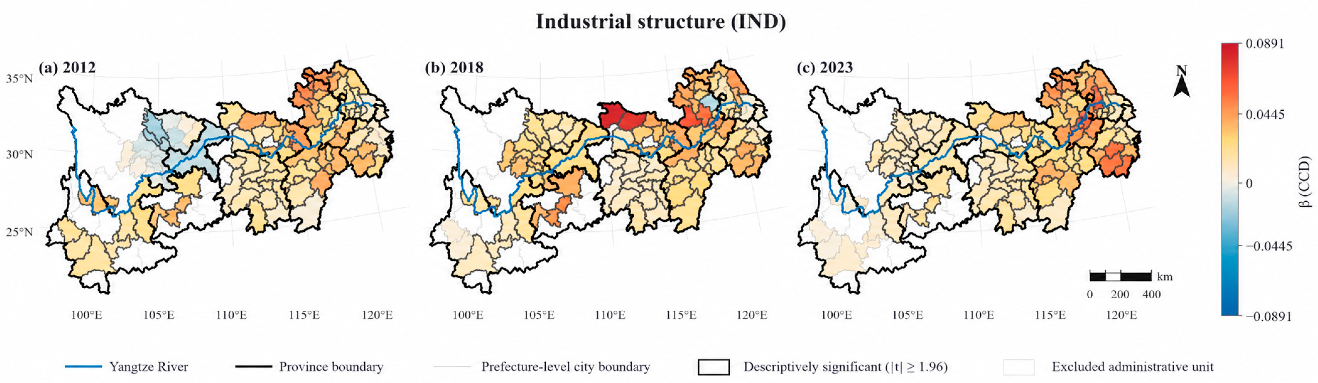
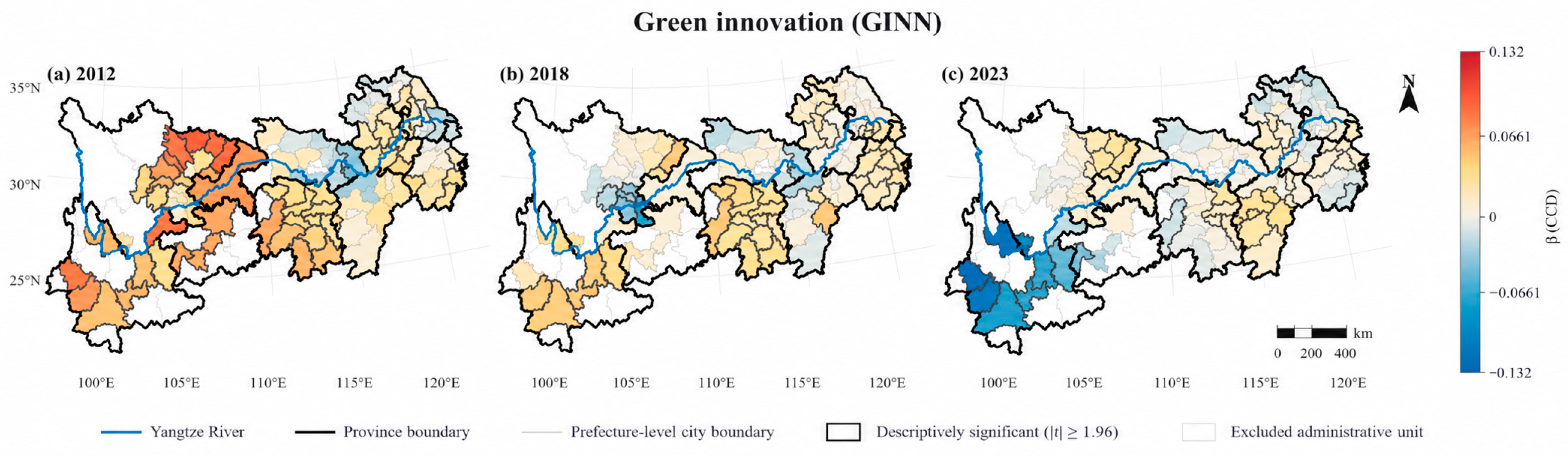
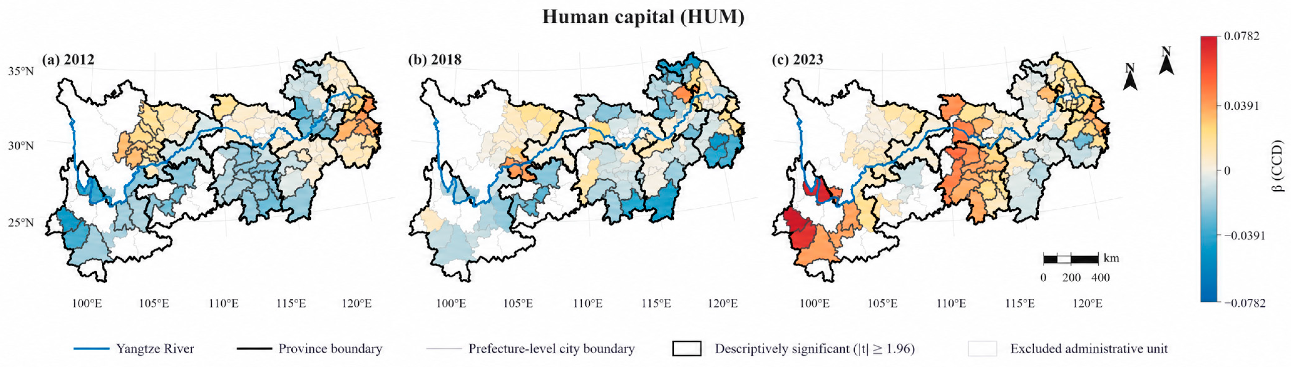
Table 6 summarizes the full coefficient distributions and reach-specific medians. Figure 4, Figure 5, Figure 6 and Figure 7 display the estimated local coefficients for all sampled cities using polygon fill colors, while bold city outlines separately identify locations meeting the descriptive |t| ≥ 1.96 screen. Administrative units excluded from the harmonized sample are shown in white. This separation prevents the apparent spatial extent of the coefficient surface from being conflated with the precision screen. The screen remains descriptive only and is not a simultaneous or multiple-testing-adjusted inference.
Table 6.
Distribution and reach-specific medians of local coefficients in the stability-selected CCD-GTWR specification.
Figure 4.
Local GTWR coefficients for economic development (ECON): (a) 2012; (b) 2018; (c) 2023. Note: Polygon colors show local coefficients for all sampled cities; bold outlines mark |t| ≥ 1.96. White polygons represent excluded administrative units. The screen is descriptive and not adjusted for multiple testing. The same convention applies to Figure 5, Figure 6 and Figure 7.
Economic development (ECON) shows the most consistently positive local association with CCD. Across all city–year estimates, 98.7% of coefficients are positive; the median is 0.0419 and the interquartile range is 0.0292–0.0623. Reach medians increase from 0.0355 in the upper reach to 0.0410 in the middle reach and 0.0491 in the lower reach. Across the three mapped years, the median local coefficient rises from 0.0345 in 2012 to 0.0465 in 2018 and 0.0563 in 2023. Figure 4 shows the coefficient values for all cities rather than coloring only locations that pass the |t| screen. The broad positive pattern is therefore visible independently of the precision overlay and is consistent with the role of economic capacity in supporting infrastructure, public services, and governance resources required by both transitions.
Industrial upgrading (IND) is likewise predominantly positive: 97.3% of all coefficients are above zero, with a median of 0.0236 and an interquartile range of 0.0133–0.0368. Reach medians are 0.0171, 0.0251, and 0.0316 for the upper, middle, and lower groups, respectively. The key-year medians are comparatively stable (0.0207 in 2012, 0.0221 in 2018, and 0.0208 in 2023), while the positive-coefficient share rises from 86.1% to 100%. Figure 5 therefore supports a persistent positive spatial association more clearly than a monotonic strengthening of coefficient magnitude. This pattern is consistent with evidence linking industrial upgrading to greener productivity [26,34,35], but it is not interpreted as a within-city causal effect.
Figure 5.
Local GTWR coefficients for industrial upgrading (IND): (a) 2012; (b) 2018; (c) 2023.
Green innovation (GINN) is more heterogeneous. Its overall median is 0.0136, the interquartile range crosses zero (−0.0051 to 0.0304), and 68.7% of local coefficients are positive. The upper-reach median (0.0238) exceeds those of the middle (0.0105) and lower (0.0130) reaches. Across the mapped years, however, the median declines from 0.0272 in 2012 to 0.0122 in 2018 and 0.0049 in 2023, while the positive share falls from 77.8% to 61.1%. Figure 6 therefore indicates context-dependent and evolving local associations rather than a uniformly strengthening green-innovation channel. Related studies on digital finance, digitalization, and green innovation provide mechanism-consistent context [27,31,33,36], but the present surface remains descriptive and no formal simultaneous nonstationarity test is used.
Figure 6.
Local GTWR coefficients for green innovation (GINN): (a) 2012; (b) 2018; (c) 2023.
Human capital (HUM) is nearly balanced in sign over the full panel, with a median of 0.0003, an interquartile range of −0.0138 to 0.0132, and 50.5% positive coefficients. Reach medians are 0.0049 in the upper group, −0.0031 in the middle group, and 0.0008 in the lower group. The key-year pattern is non-monotonic: the median is 0.0022 in 2012, −0.0036 in 2018, and 0.0118 in 2023, while the positive share rises to 75.9% in 2023. Figure 7 thus supports a later-period shift toward more positive local associations but not a stable full-period effect. ER and OPEN also have small, mixed coefficients in Table 6, reinforcing the view that institutional pressure and external connectivity depend strongly on local industrial and governance conditions.
Figure 7.
Local GTWR coefficients for human capital (HUM): (a) 2012; (b) 2018; (c) 2023.
4.5. Robustness and Model Validation
Measurement robustness is first assessed against alternative weighting and dominant-indicator choices. Re-estimating DIG, GRE, and CCD using CRITIC rather than entropy weights produces correlations of 0.966, 0.994, and 0.983, respectively, between annual mean series; city–year CCD rankings have a Spearman correlation of 0.987. Varying the DIG/GRE weights in the composite development term from 0.5/0.5 to 0.4/0.6 or 0.6/0.4 leaves the city–year Spearman correlation above 0.999 and the annual-mean correlation above 0.9999. Deleting digital patents alone yields a CCD Spearman correlation of 0.995, while deleting both digital patents and AI-related firm density still yields a Spearman correlation of 0.987 and an annual-mean correlation of 0.988. These checks concern ranking and measurement stability; they do not alter the algebraic point that equal-weight CCD is interpreted as symmetric joint development while C is reported separately for balance.
Missing-data sensitivity is examined directly. Recalculating Global Moran’s I using only cities for which all 19 DIG/GRE input indicators were directly observed in each selected year preserves the finding of positive spatial autocorrelation, although changes in sample membership and the corresponding spatial weight matrix prevent a like-for-like assessment of the size of any interpolation effect: for 2012, 2016, 2018, 2021, and 2023, the direct-observation samples contain 82–85 cities and yield Moran’s I values of 0.517, 0.473, 0.428, 0.371, and 0.368, respectively, with permutation p = 0.001 in every case. A stricter complete-case check retains 996 city–year observations, where all 25 core variables were directly observed, and re-estimates GTWR with the same processing and bandwidth; R2 is 0.9751 versus 0.9746 in the full sample. Appendix A Table A3 shows that the focal coefficient medians and positive shares also remain close. Removing the three indicators with the highest imputation concentration likewise leaves the annual CCD series highly correlated with the baseline (r = 0.985).
Spatial-weight sensitivity produces a similarly clear distinction between robust and matrix-specific conclusions. The fixed 165.75 km distance-band matrix closely reproduces the KNN pattern, with an annual Moran-series correlation of 0.975. Inverse-distance, economic-similarity, and geo-economic matrices all retain positive and highly significant annual spatial autocorrelation, but their temporal profiles are flatter. Positive spatial dependence is therefore robust to the matrix definition, whereas the precise magnitude and rate of temporal weakening are not treated as invariant.
Bandwidth sensitivity directly tests whether the stability-selected k = 60 specification suppresses the substantive local patterns revealed by the more local k = 28 solution. Some smoothing is measurable: the standard deviation of the six coefficient surfaces falls by 20.9–53.7% under k = 60. Nevertheless, ECON and IND remain highly stable, with k28–k60 Pearson correlations of 0.835 and 0.821, sign agreement of 94.7% and 93.8%, and nearly unchanged medians (0.0430 versus 0.0419 for ECON; 0.0229 versus 0.0236 for IND). GINN is moderately stable, whereas HUM, ER, and especially OPEN are more bandwidth-sensitive; OPEN has the lowest cross-bandwidth correlation (0.539) and the largest reduction in dispersion. The main ECON and IND sign patterns are consequently similar across the two bandwidths, although k = 60 measurably smooths the coefficient surfaces; the more variable local estimates are interpreted more cautiously.
Global panel benchmarks clarify what the local GTWR surfaces do and do not identify. Table 7 reports pooled OLS, a year-demeaned regression that removes common annual shocks, and TWFE with city and year fixed effects; all standard errors are clustered by city. ECON, IND, and GINN remain positive in the year-demeaned model, indicating that their pooled associations are not explained solely by common time shocks. In TWFE, however, ECON and IND attenuate to statistically insignificant within-city coefficients, GINN remains positive, and HUM becomes negative. Table 7 now also reports N and specification-specific fit statistics; these are not used to rank the global models because pooled, demeaned, and within-city R2 values describe different sources of variation. This coefficient contrast is consistent with a substantial role for persistent cross-city differences and local spatial structure in the positive ECON and IND GTWR surfaces, but it does not identify the precise source of the difference between estimators or establish a zero within-city causal effect. GTWR is therefore retained as a descriptive heterogeneity model, not as a causal panel estimator.
Table 7.
Global panel robustness benchmarks for CCD, with sample size and specification-specific fit statistics.
A construction-overlap check addresses the potential mechanical link between ECON and the GDP-normalized intensity indicators in GRE. After dropping electricity, water, CO2, SO2, wastewater, and smoke/dust intensities and re-estimating entropy weights over the five remaining GRE indicators, the alternative CCD remains extremely close to the baseline (city–year Spearman ρ = 0.9965; annual-mean Pearson r = 0.9996). The pooled ECON coefficient is 0.0625 compared with 0.0615 in the baseline, the TWFE ECON coefficient is 0.0088 compared with 0.0076 and remains statistically insignificant, and the stability-selected GTWR ECON surface has a median coefficient of 0.0409 with 97.2% positive local coefficients, compared with 0.0419 and 98.7% in the baseline. The cross-city ECON surface is therefore not driven primarily by GDP appearing in the six excluded GRE denominators, while the TWFE result continues to caution against causal within-city interpretation. Table 8 reports the blocked predictive sensitivity results across city, year, reach, and contiguous-period removal schemes.
Table 8.
Blocked predictive sensitivity RMSE for the four benchmark models under city, year, reach, and contiguous-period removal.
Blocked validation adds a final transportability stress test. Table 8 confirms the previously reported trade-off for unseen cities and years and extends it to entire reach groups and contiguous periods. When an entire city is withheld, TWR has the lowest RMSE (0.0291), followed by GTWR (0.0386). When an entire year is withheld, GTWR is best (0.0215). The new leave-one-reach-out test is intentionally severe: TWR is best overall (0.0355) and pooled OLS is second (0.0471), whereas GTWR rises to 0.1084 and GWR-type to 0.1910; the loss of nearby training support is one plausible contributor, alongside possible model instability under spatial extrapolation. The upper-reach holdout is especially difficult: its held-out cities are a median 576.6 km from the nearest training city and GTWR RMSE reaches 0.1808. By contrast, GTWR remains best under all five contiguous two-year period blocks, with a pooled RMSE of 0.0214 compared with 0.0238 for GWR-type, 0.0315 for TWR, and 0.0466 for OLS. Under these fixed-specification stress tests, GTWR performs comparatively well for held-out years and contiguous time blocks, but extrapolates poorly to wholly unseen reaches; the checks do not establish fully prospective predictive transportability. Together with the residual-Moran diagnostics, they support GTWR as a compact descriptive model for sample-supported spatiotemporal surfaces without implying universal forecasting superiority or causal identification.
5. Discussion
5.1. Sustained Improvement, a Sample-Period Dispersion Minimum Around 2018, and Renewed Dispersion
The results first confirm sustained improvement in digitalization, green development, and CCD-based joint development, consistent with several related Chinese urban studies [13,14,15,17]. Mean C also rises from 0.5312 to 0.7745, indicating improved average relative balance between the two constructed subsystem indices. KDE adds information that is invisible in either mean measure. From 2012 to 2018, the CCD distribution shifts rightward and becomes modestly more concentrated, indicating distributional compression rather than a formal β- or σ-convergence test. Dispersion reaches its sample-period minimum around 2018 and then increases while the distribution continues to move rightward and develops a longer upper tail. The timing is descriptive: 2018 is the observed minimum in this sample, not a formally estimated structural-break date.
This combination of a rising mean and renewed dispersion may reflect scale and network effects in digital development. One plausible interpretation, consistent with the broader literature, is that lower-reach core cities more often combine stronger digital-finance capacity, AI-related enterprise concentration, innovation activity, and modern services with relatively established green-governance and public-service systems. Such complementarities could help explain their faster later-period improvement, but the present analysis does not formally decompose the reach-level gap into these channels. Cities in the middle- and upper-reach groups also improve, while differences in digital-industry foundations, talent attraction, innovation networks, and industrial transformation may contribute to increasingly differentiated trajectories. Within this sample, the post-2018 widening is therefore consistent with more differentiated capability-dependent trajectories, not evidence of a discrete structural regime shift.
5.2. Falling Overall Inequality Can Coexist with a Stronger Regional Gradient
The Dagum results show that the 2023 overall Gini remains well below its 2012 value even though the net between-region contribution approaches 50%. These findings are not contradictory. In the early period, each reach contained a relatively wide mix of low- and medium-to-high-CCD cities, so regional distributions overlapped strongly. As very low CCD values became less common, overall inequality fell. At the same time, the faster later-period rightward shift of lower-reach cities increased the importance of differences between reaches in the inequality that remained. The declining transvariation share is interpreted as reduced distributional overlap among reach groups, not as evidence that geographic boundary cities are the source of the remaining inequality.
The consistently positive Moran’s I further indicates that geographic proximity remains relevant to the distribution of CCD. Under the baseline KNN and fixed distance-band matrices, Moran’s I declines clearly over the sample period, whereas denser alternative matrices remain positive and significant but show flatter temporal trends. Persistent positive spatial dependence is therefore more robust than the exact degree of temporal weakening. This pattern is consistent with the territorial embeddedness of regional innovation and production systems [1,2]. Because Global Moran’s I does not identify directional spillovers or diffusion mechanisms, the policy implication is limited to the value of cross-jurisdictional coordination and shared regional monitoring rather than a claim that improvements automatically diffuse to neighboring cities.
5.3. Why the Local Associations Differ in Spatiotemporal Stability
The benchmark model comparison clarifies why the local associations are interpreted in a joint spatiotemporal framework. Pooled OLS leaves substantial residual spatial dependence, TWR does not remove that dependence, and the spatial-only GWR-type model improves the residual pattern but at much higher effective complexity. Within the GTWR family, the pure-CV k = 28 specification has a slightly lower ordinary LOOCV error, whereas the stability-selected k = 60 specification has larger effective neighborhoods, lower local condition numbers, and lower AICc values. ECON and IND remain strongly concordant across the two bandwidths, while HUM, ER, and especially OPEN are more bandwidth-sensitive. Fixed-specification blocked sensitivity checks also show task-specific performance: GTWR has the lowest RMSE for held-out years and contiguous two-year periods, whereas TWR performs best when entire cities or reaches are withheld. At the same time, the panel robustness results qualify the substantive interpretation: year demeaning preserves positive ECON, IND, and GINN associations, but TWFE attenuates ECON and IND, a contrast consistent with persistent cross-city and spatial differences playing a role in the GTWR surfaces, without isolating their contribution causally. These contrasts caution against reading any local coefficient as a causal treatment effect or assuming that local surfaces transport to wholly unseen regions.
Green innovation and human capital show stronger descriptive variation across space and time. Digital-finance studies indicate that financing conditions can influence green innovation [27,31], while city-level evidence links digital-economy development to green innovation [33]; human capital can also condition the emissions implications of green technology innovation [36]. These findings provide a mechanism-consistent context for why GINN may display mixed local associations with CCD, but they do not directly identify the mechanisms operating in this study. Among the three mapped years, the 2023 human-capital coefficient surface is more often positive than the 2018 surface; this is a descriptive comparison of local estimates, not a test of change in statistical significance. The pattern is consistent with evidence linking human capital to green technology innovation [37] and spatial green-growth convergence [38]. The mixed ER and OPEN surfaces may be consistent with contextual variation related to industrial structure, development stage, and governance conditions, although these conditioning mechanisms are not directly tested. Their greater bandwidth sensitivity, especially for OPEN, reinforces the need for cautious interpretation. These are mechanism-consistent readings of descriptive coefficients rather than direct tests of the mechanisms themselves.
5.4. Contributions and Limitations
The study contributes an integrated multiscale diagnostic centered on one consistently constructed CCD measure. Under the equal-weight specification used here, CCD is interpreted as a symmetric joint-development summary, while the coupling degree (C) is reported separately as the balance diagnostic. KDE identifies changes in distributional location and dispersion; Dagum decomposition identifies where inequality originates; Moran’s I evaluates spatial clustering; benchmark OLS/GWR-type/TWR/GTWR comparisons justify the local model; and GTWR maps descriptive spatiotemporal association surfaces. The additional measurement, imputation, alternative-spatial-matrix, bandwidth-stability, panel, and blocked predictive sensitivity checks make explicit which findings are robust and which depend on specification or support. Digital–green coordination is therefore treated not simply as a rising index but as a dynamic process with distributional, regional, spatial, and local heterogeneity [1,2,3,4].
Several limitations remain. First, GTWR identifies heterogeneous conditional associations, not causal effects. The TWFE benchmark shows that some strong spatial associations, particularly for ECON and IND, weaken when identification is restricted to within-city changes; future work could combine the present spatial diagnostics with quasi-natural experiments based on digital-infrastructure, low-carbon, or related policy shocks. Second, the 108-city analytical universe does not include every prefecture-level administrative unit in the YREB. Sixteen of the 18 exclusions are in the upper-reach group, so the regional comparison may underrepresent conditions in less urbanized autonomous-prefecture areas; the leave-one-reach-out validation also shows that local spatial models transport poorly when an entire region is outside the estimation support. The reported reach-group results therefore generalize to the harmonized city-type sample rather than the full administrative universe. Third, equal-weight CCD does not independently identify subsystem balance, which is why C is reported separately. Entropy weights capture sample-specific information dispersion rather than normative importance, and the AI-related enterprise indicator represents a broad registration-based digital-ecosystem proxy rather than a census of active AI-specialist firms.
Fourth, although the overall imputation rate is modest, missingness is uneven across variables. Direct-observation Moran tests and complete-case validation substantially reduce, but cannot eliminate, this concern. Fifth, the magnitude and temporal trend of Moran’s I depend somewhat on the spatial matrix, and the mixed HUM, ER, and OPEN surfaces show greater bandwidth sensitivity than ECON and IND. These results should therefore be interpreted as conditional spatial diagnostics rather than invariant structural parameters. Finally, city-level data cannot reveal heterogeneity among firms, industrial parks, or households; future work could use micro-level or finer spatial data to investigate the mechanisms underlying the local patterns observed here.
6. Conclusions and Policy Implications
6.1. Main Conclusions
Using panel data for 108 YREB cities from 2012 to 2023, this study combines entropy weighting, CCD-based joint-development measurement, KDE, Dagum Gini decomposition, Global Moran’s I, and GTWR to examine the temporal evolution, distributional dynamics, regional inequality, spatial dependence, and local correlates of digital–green coordination. Four conclusions emerge.
First, digitalization, green development, and CCD all increase over the sample period. CCD rises from 0.3622 to 0.5747. The separately reported coupling degree (C) rises from 0.5312 to 0.7745, indicating improved average relative balance on the constructed DIG and GRE index scales. On the constructed composite-index scales, DIG shows the largest upward movement from its lower initial mean, while GRE also improves throughout the period.
Second, the CCD distribution shifts consistently to the right, but its dispersion changes over the sample period. All three central quartiles move upward, while dispersion reaches its sample-period minimum around 2018 and increases thereafter, with lower-reach cities improving more rapidly. Dagum Gini results show the same broad pattern: inequality first falls and then increases moderately, remaining below its 2012 level in 2023, while the net between-region contribution rises to nearly 50%. The 2018 timing is descriptive rather than a formally estimated structural break.
Third, CCD exhibits significant positive spatial autocorrelation in every sample year. Under the baseline KNN matrix, Moran’s I falls from 0.5118 in 2012 to 0.4185 in 2023, and the fixed distance-band alternative shows a very similar decline. Denser alternative matrices remain positive and significant but show flatter temporal trends. Thus, persistent positive spatial dependence is robust, while the degree of temporal weakening depends on the spatial-weight specification.
Fourth, the benchmark model comparison supports joint spatiotemporal weighting for descriptive local analysis. Within GTWR, the k = 28 specification has a slightly lower ordinary LOOCV error, while the stability-selected k = 60 specification provides substantially stronger local stability; the main ECON and IND patterns remain highly concordant across the two bandwidths. Blocked predictive sensitivity checks add an important qualification: GTWR yields the lowest RMSE for unseen years and contiguous two-year period blocks, whereas TWR performs best when entire cities or reaches are withheld. Economic development and industrial upgrading show the most consistently positive local surfaces, while green innovation, human capital, environmental regulation, and openness are more heterogeneous or bandwidth-sensitive. The GDP-denominator exclusion test leaves the ECON surface essentially unchanged, but TWFE still attenuates ECON and IND to statistically insignificant within-city coefficients. The local maps should therefore be interpreted as descriptive spatiotemporal associations rather than causal within-city effects or relationships that necessarily transport to wholly unseen regions.
6.2. Policy Implications
First, digital–green coordination monitoring should be distribution-sensitive. Annual mean CCD should be supplemented with the separately reported coupling degree (C), changes in distributional dispersion, the sources of regional inequality, and spatial clustering so that improvements in the mean are not interpreted as uniform progress.
Second, the observed regional differences support differentiated diagnosis rather than a uniform policy package. Lower-reach cities may prioritize identifying remaining bottlenecks in technology integration, standards, and inter-city knowledge exchange, whereas middle- and upper-reach cities may prioritize diagnosing gaps in digital infrastructure, green public services, absorptive capacity, and industrial transition. Which intervention is effective in a particular city is not identified causally by the present analysis. These recommendations follow from observed regional differences and spatial clustering, not from an estimated causal spillover mechanism.
Third, industrial and digital–green policies should be coordinated rather than treated as independent levers. The positive spatial association between industrial upgrading and CCD indicates that more upgraded urban economies also tend to exhibit higher CCD-based joint development, but the TWFE attenuation means this pattern should not be interpreted as evidence that industrial upgrading alone will raise CCD within a city. Policy packages for manufacturing digitalization, smart energy management, green supply chains, and data-supported environmental governance should therefore be evaluated jointly and, where possible, with causal policy designs.
Fourth, green-innovation and human-capital policy should be adapted to local conditions and preceded by diagnosis, rather than inferred mechanically from coefficient signs. Cities showing weak or negative local green-innovation associations may warrant closer examination of technology commercialization, absorptive capacity, digital infrastructure, and industrial structure before additional interventions are selected. Where independent evidence identifies skill bottlenecks, workforce strategies may emphasize hybrid capabilities in smart manufacturing, carbon-data management, green algorithms, and environmental monitoring. The effectiveness of such interventions should be evaluated separately from the descriptive GTWR relationships.
Author Contributions
Conceptualization, K.D. and H.L.; methodology, K.D. and H.L.; validation, K.D.; formal analysis, K.D.; investigation, K.D.; data curation, K.D. and H.L.; writing—original draft preparation, K.D. and H.L.; writing—review and editing, H.L.; project administration, K.D. All authors have read and agreed to the published version of the manuscript.
Funding
This work was supported by the Ministry of Education of the Republic of Korea and the National Research Foundation of Korea (NRF-2025S1A5A2A01007457).
Institutional Review Board Statement
Not applicable.
Informed Consent Statement
Not applicable.
Data Availability Statement
The data presented in this study are available on request from the corresponding author due to third-party licensing and redistribution restrictions. The analysis combines data from multiple providers, and requests for the processed data will be handled in accordance with the applicable provider terms. The related analysis code, GTWR bandwidth grid, and variable documentation are available from the corresponding author upon reasonable request.
Acknowledgments
During the preparation of this manuscript, the authors used ChatGPT (GPT-5.6 model, OpenAI) for English translation and editing, statistical-code drafting and debugging for robustness and consistency checks, and document-formatting support. The tool was not used as a source of empirical data or bibliographic authority. All analytical decisions, data preparation, computations, reference verification, interpretation, and the final text were reviewed by the authors, who take full responsibility for the publication.
Conflicts of Interest
The authors declare no conflicts of interest.
Appendix A. Additional Spatial and Robustness Diagnostics
The appendix is intentionally limited to diagnostics that directly support the spatial and robustness claims in the main text. In addition to the original annual Moran, residual-Moran, and complete-case diagnostics, it reports variable-level missingness, the full GTWR bandwidth grid, and alternative spatial-weight sensitivity. Detailed source files, the city crosswalk, and cell-level imputation logs are available from the corresponding author upon reasonable request.
Table A1.
Annual Global Moran’s I for CCD, 2012–2023.
Table A2.
Annual residual Global Moran’s I for benchmark models, 2012–2023.
Table A3.
Full-sample versus complete-case GTWR coefficient summaries for focal covariates.
Table A4.
Variables with missing observations in the 25-variable analytical panel.
Table A5.
Full 77-combination GTWR AICc bandwidth grid (τ in km/year).
Table A6.
Annual Global Moran’s I under alternative spatial-weight matrices.
References
- Faggian, A.; Marzucchi, A.; Montresor, S. Regions facing the ‘twin transition’: Combining regional green and digital innovations. Reg. Stud. 2025, 59, 2398555. [Google Scholar] [CrossRef] [Scilit]
- Brueck, C.; Losacker, S.; Liefner, I. China’s digital and green (twin) transition: Insights from national and regional innovation policies. Reg. Stud. 2025, 59, 2384411. [Google Scholar] [CrossRef] [Scilit]
- Bruno, R.L.; Jin, J.; Korosteleva, J.; Liu, Y.; Radosevic, S.; Wang, Z. A critical evaluation of digitalisation and green measures for advancing twin transition metrics. Discov. Sustain. 2026, 7, 1233. [Google Scholar] [CrossRef] [Scilit]
- Al-Silefanee, R.; Uctu, R.; Koc, S. The twin transition and carbon emissions per capita: Digital–green complementarities and configuration effects. Int. J. Innov. Stud. 2026, 100225. [Google Scholar] [CrossRef] [Scilit]
- Zhao, T.; Zhang, Z.; Liang, S. Digital economy, entrepreneurship, and high-quality economic development: Empirical evidence from urban China. J. Manag. World 2020, 36, 65–76. [Google Scholar] [CrossRef]
- Xiao, Y.; Wu, S.; Liu, Z.Q.; Lin, H.J. Digital economy and green development: Empirical evidence from China’s cities. Front. Environ. Sci. 2023, 11, 1124680. [Google Scholar] [CrossRef] [Scilit]
- Guo, D.; Li, L.; Pang, G. Does the integration of digital and real economies promote urban green total factor productivity? Evidence from China. J. Environ. Manag. 2024, 370, 122934. [Google Scholar] [CrossRef] [Scilit] [PubMed]
- Liu, Y.; Xie, Y.; Zhong, K. Impact of digital economy on urban sustainable development: Evidence from Chinese cities. Sustain. Dev. 2024, 32, 307–324. [Google Scholar] [CrossRef] [Scilit]
- Liao, W. How does the digital economy affect the development of the green economy? Evidence from Chinese cities. PLoS ONE 2023, 18, e0289826. [Google Scholar] [CrossRef] [Scilit] [PubMed]
- Lange, S.; Pohl, J.; Santarius, T. Digitalization and energy consumption. Does ICT reduce energy demand? Ecol. Econ. 2020, 176, 106760. [Google Scholar] [CrossRef] [Scilit]
- Belkhir, L.; Elmeligi, A. Assessing ICT global emissions footprint: Trends to 2040 & recommendations. J. Clean. Prod. 2018, 177, 448–463. [Google Scholar] [CrossRef] [Scilit]
- Freitag, C.; Berners-Lee, M.; Widdicks, K.; Knowles, B.; Blair, G.S.; Friday, A. The real climate and transformative impact of ICT: A critique of estimates, trends, and regulations. Patterns 2021, 2, 100340. [Google Scholar] [CrossRef] [Scilit] [PubMed]
- She, Q.; Qian, J.; He, L. Research on the relationship of coupling coordination between digitalization and green development. Sci. Rep. 2024, 14, 19569. [Google Scholar] [CrossRef] [Scilit] [PubMed]
- Zhong, X.; Duan, Z.; Liu, C.; Chen, W. Research on the coupling mechanism and influencing factors of digital economy and green technology innovation in Chinese urban agglomerations. Sci. Rep. 2024, 14, 5150. [Google Scholar] [CrossRef] [Scilit] [PubMed]
- Yu, T.; Zhang, Y.; Jia, S.; Cui, X. Spatio-temporal evolution and drivers of coupling coordination between digital infrastructure and inclusive green growth: Evidence from the Yangtze River Economic Belt. J. Environ. Manag. 2025, 376, 124416. [Google Scholar] [CrossRef] [Scilit] [PubMed]
- Yang, X.; Ran, G. Factors influencing the coupled and coordinated development of cities in the Yangtze River Economic Belt: A focus on carbon reduction, pollution control, greening, and growth. J. Environ. Manag. 2024, 370, 122499. [Google Scholar] [CrossRef] [Scilit] [PubMed]
- Liu, Y. Coupling and coordination evaluation of digital economy and green development efficiency in eight urban agglomerations in China. Sci. Rep. 2025, 15, 26829. [Google Scholar] [CrossRef] [Scilit] [PubMed]
- Meng, G.; Wang, K.; Wang, F.; Li, H. Spatial-temporal pattern and mechanism of the coupling coordination relationship between digital economy and urban-rural integration development at prefectural level in the Yangtze River Economic Belt. Econ. Geogr. 2024, 44, 73–83. [Google Scholar] [CrossRef]
- Li, P.; Ding, X.; Guo, T. How the integration of technology and finance empowers the collaborative development of digitalization and greenization of Chinese cities. J. Innov. Knowl. 2026, 15, 101006. [Google Scholar] [CrossRef] [Scilit]
- Dagum, C. A new approach to the decomposition of the Gini income inequality ratio. Empir. Econ. 1997, 22, 515–531. [Google Scholar] [CrossRef] [Scilit]
- Moran, P.A.P. Notes on continuous stochastic phenomena. Biometrika 1950, 37, 17–23. [Google Scholar] [CrossRef] [Scilit]
- Huang, B.; Wu, B.; Barry, M. Geographically and temporally weighted regression for modeling spatio-temporal variation in house prices. Int. J. Geogr. Inf. Sci. 2010, 24, 383–401. [Google Scholar] [CrossRef] [Scilit]
- Fotheringham, A.S.; Brunsdon, C.; Charlton, M. Geographically Weighted Regression: The Analysis of Spatially Varying Relationships; Wiley: Chichester, UK, 2002. [Google Scholar]
- Yuan, H.; Liu, J.; Li, X.; Zhong, S. The impact of digital economy on environmental pollution: Evidence from 267 cities in China. PLoS ONE 2024, 19, e0297009. [Google Scholar] [CrossRef] [PubMed]
- Yang, S.; Li, H.; Liu, X.; Wei, Y.; Shen, J.; Cheng, B. Spatial analysis of the digital economy’s influence on urban sustainable development: A decade-long study of Chinese prefecture-level cities. Ecol. Indic. 2024, 166, 112338. [Google Scholar] [CrossRef] [Scilit]
- Liu, Y.; Yang, Y.; Li, H.; Zhong, K. Digital economy development, industrial structure upgrading and green total factor productivity: Empirical evidence from China’s cities. Int. J. Environ. Res. Public Health 2022, 19, 2414. [Google Scholar] [CrossRef] [Scilit] [PubMed]
- Feng, S.; Zhang, R.; Li, G. Environmental decentralization, digital finance and green technology innovation. Struct. Change Econ. Dyn. 2022, 61, 70–83. [Google Scholar] [CrossRef] [Scilit]
- He, Z.; Chen, H.; Hu, J.; Zhang, Y. The impact of digital inclusive finance on provincial green development efficiency: Empirical evidence from China. Environ. Sci. Pollut. Res. 2022, 29, 90404–90418. [Google Scholar] [CrossRef] [Scilit] [PubMed]
- Han, Y.; Li, Y.; Wang, Q. Digital finance, environmental regulation, and green development efficiency of China. Front. Environ. Sci. 2023, 11, 1131058. [Google Scholar] [CrossRef] [Scilit]
- Yang, S.; Xu, J.; Lei, T.; Wang, M. How to improve the efficiency of green development? The role of digital finance. Financ. Res. Lett. 2024, 63, 105296. [Google Scholar] [CrossRef] [Scilit]
- Xu, R.; Yao, D.; Zhou, M. Does the development of digital inclusive finance improve the enthusiasm and quality of corporate green technology innovation? J. Innov. Knowl. 2023, 8, 100382. [Google Scholar] [CrossRef] [Scilit]
- Zhuang, R.; Mi, K.; Zhi, M.; Zhang, C. Digital finance and green development: Characteristics, mechanisms, and empirical evidences. Int. J. Environ. Res. Public Health 2022, 19, 16940. [Google Scholar] [CrossRef] [Scilit] [PubMed]
- Wei, S.; Du, J.; Pan, S. How does digital economy promote green innovation? Empirical evidence from Chinese cities. China Econ. Transit. 2022, 5, 408–427. [Google Scholar] [CrossRef]
- Tian, X.; Zhang, H. Analysis of the impact factors of industrial structure upgrading on green total factor productivity from the perspective of spatial spillover effects. Heliyon 2024, 10, e28660. [Google Scholar] [CrossRef] [Scilit] [PubMed]
- Sun, J.; Tang, D.; Kong, H.; Boamah, V. Impact of industrial structure upgrading on green total factor productivity in the Yangtze River Economic Belt. Int. J. Environ. Res. Public Health 2022, 19, 3718. [Google Scholar] [CrossRef] [Scilit] [PubMed]
- Wu, K.; Geng, Y.; Guo, T. The impact of green technology innovation on carbon emissions from the perspective of urban agglomeration: The moderating effect of human capitals. J. Nat. Resour. 2024, 39, 2121–2139. [Google Scholar] [CrossRef] [Scilit]
- Zhang, J.; Li, S. The impact of human capital on green technology innovation—Moderating role of environmental regulations. Int. J. Environ. Res. Public Health 2023, 20, 4803. [Google Scholar] [CrossRef] [Scilit] [PubMed]
- Lin, X. The impact of innovative human capital on green growth convergence in China’s regions from the perspective of space. Heliyon 2024, 10, e34463. [Google Scholar] [CrossRef] [Scilit] [PubMed]
- Fan, F.; Lian, H.; Liu, X.; Wang, X. Can environmental regulation promote urban green innovation efficiency? An empirical study based on Chinese cities. J. Clean. Prod. 2021, 287, 125060. [Google Scholar] [CrossRef] [Scilit]
- Porter, M.E.; van der Linde, C. Toward a new conception of the environment–competitiveness relationship. J. Econ. Perspect. 1995, 9, 97–118. [Google Scholar] [CrossRef] [Scilit]
- Acemoglu, D.; Aghion, P.; Bursztyn, L.; Hemous, D. The environment and directed technical change. Am. Econ. Rev. 2012, 102, 131–166. [Google Scholar] [CrossRef] [Scilit] [PubMed]
- Yan, Y.; Li, Z.; Zhang, Y.; Wu, J.; Zhang, Y. The effects of foreign direct investment on green technology innovation: New evidence from China’s 278 cities. Emerg. Mark. Financ. Trade 2025, 61, 940–963. [Google Scholar] [CrossRef] [Scilit]
- Guo, F.; Wang, J.; Wang, F.; Kong, T.; Zhang, X.; Cheng, Z. Measuring the development of digital inclusive finance in China: Index compilation and spatial characteristics. China Econ. Q. 2020, 19, 1401–1418. [Google Scholar] [CrossRef]
- Chao, X.; Lian, Y.; Luo, L. Impact of new digital infrastructure on high-quality development of manufacturing. Financ. Trade Res. 2021, 32, 1–13. [Google Scholar] [CrossRef]
- Shannon, C.E. A mathematical theory of communication. Bell Syst. Tech. J. 1948, 27, 623–656. [Google Scholar] [CrossRef] [Scilit]
- Diakoulaki, D.; Mavrotas, G.; Papayannakis, L. Determining objective weights in multiple criteria problems: The CRITIC method. Comput. Oper. Res. 1995, 22, 763–770. [Google Scholar] [CrossRef] [Scilit]
- Kish, L. Survey Sampling; Wiley: New York, NY, USA, 1965. [Google Scholar]
- Gollini, I.; Lu, B.; Charlton, M.; Brunsdon, C.; Harris, P. GWmodel: An R package for exploring spatial heterogeneity using geographically weighted models. J. Stat. Softw. 2015, 63, 1–50. [Google Scholar] [CrossRef] [Scilit]
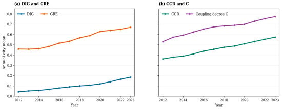
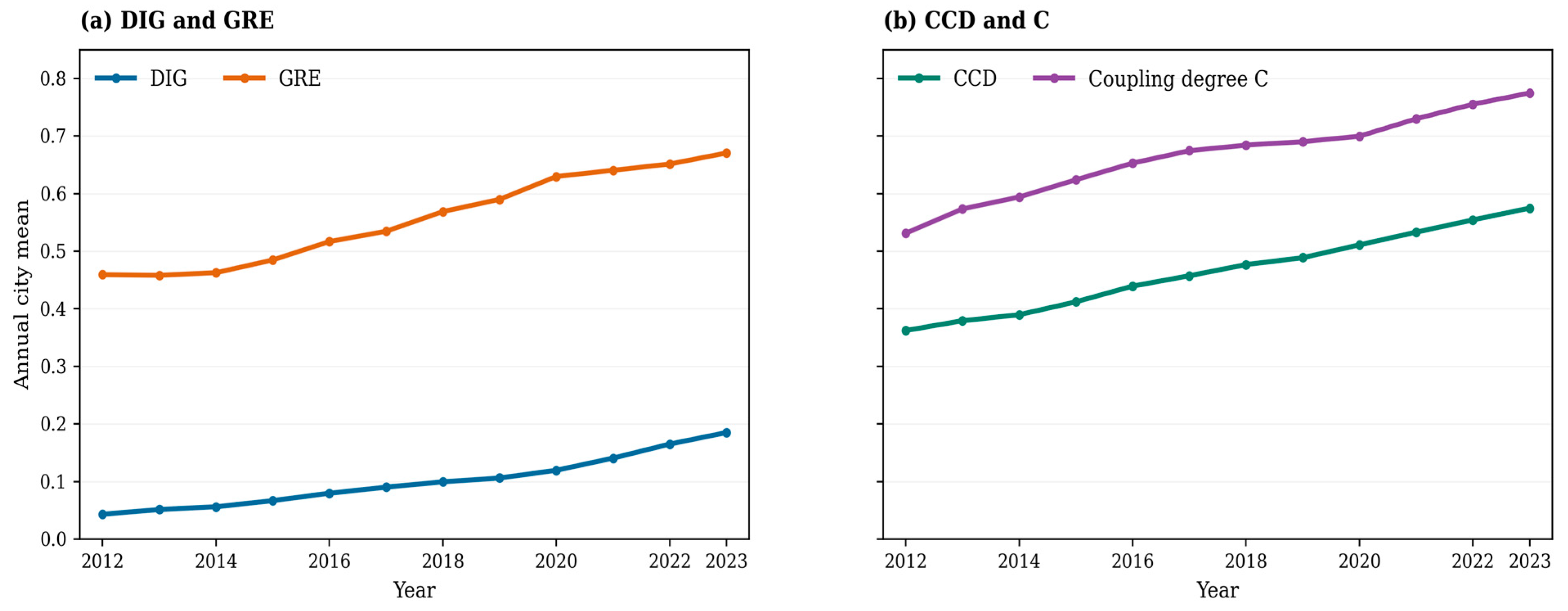
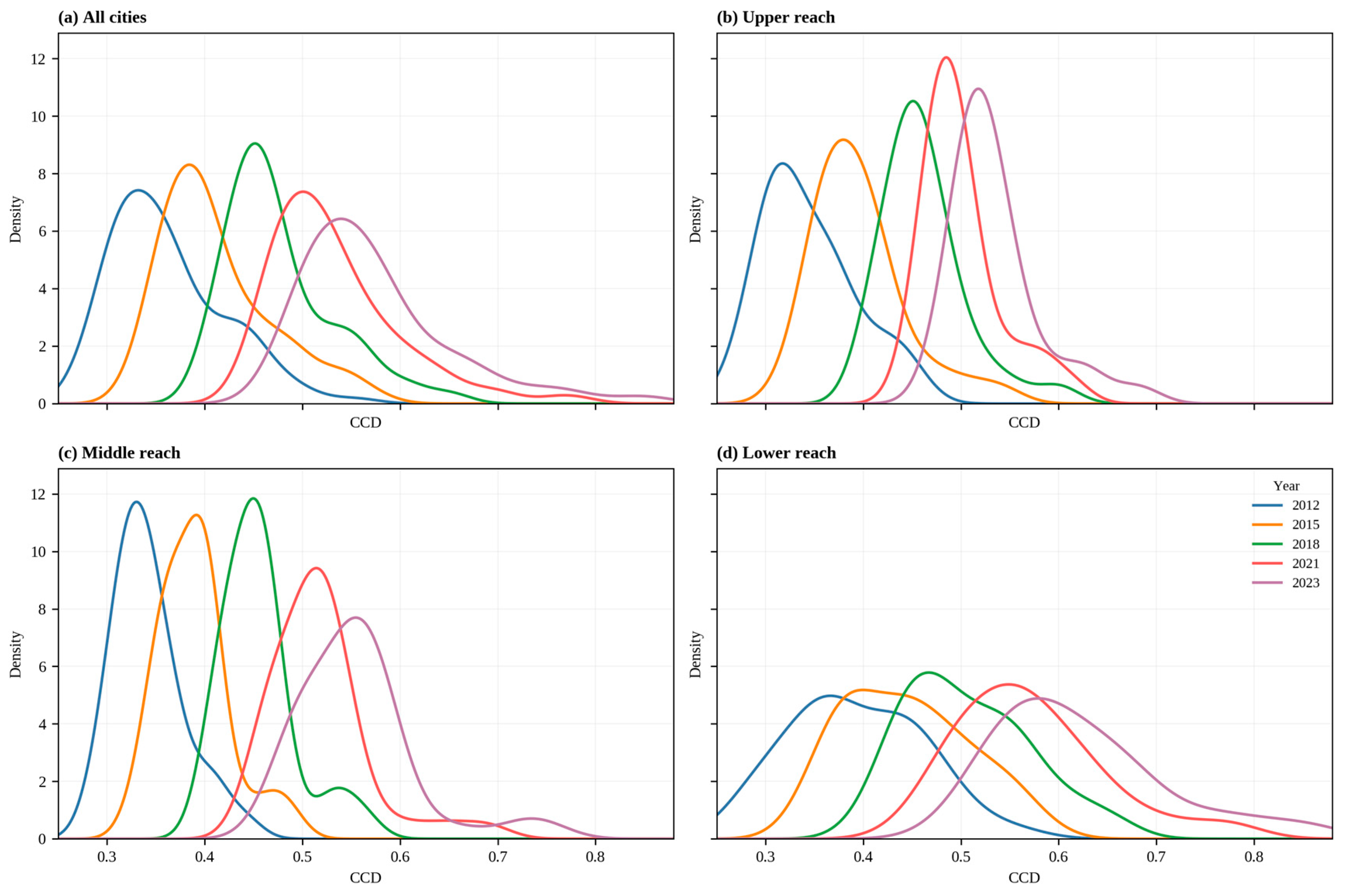
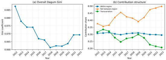
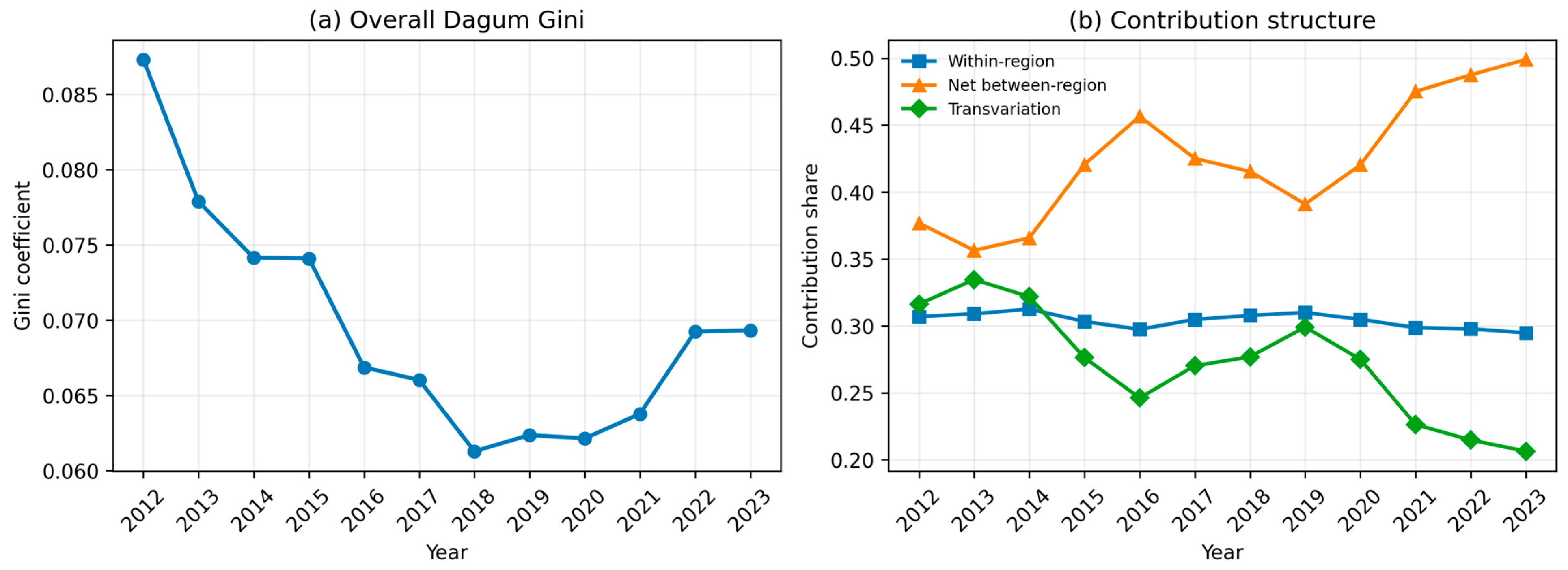
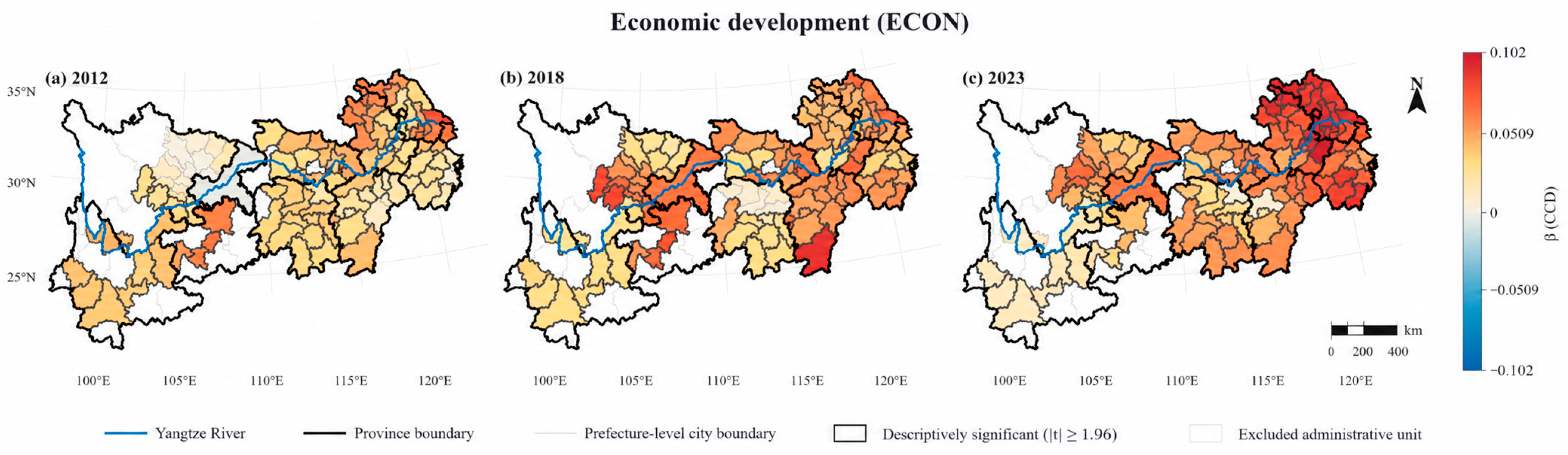

Disclaimer/Publisher’s Note: The statements, opinions and data contained in all publications are solely those of the individual author(s) and contributor(s) and not of MDPI and/or the editor(s). MDPI and/or the editor(s) disclaim responsibility for any injury to people or property resulting from any ideas, methods, instructions or products referred to in the content. |
© 2026 by the authors. Licensee MDPI, Basel, Switzerland. This article is an open access article distributed under the terms and conditions of the Creative Commons Attribution (CC BY) license.