Nexus Among Innovation, Energy, Economic Structure, and CO₂ Emissions in China: Evidence from a Bayesian Fourier ARDL Approach

Abstract

China’s carbon mitigation challenge is intricately linked to energy consumption, income growth, innovation performance, and sectoral structure. Using annual aggregate data for 1995–2021, this study investigates these dynamics using Fourier ARDL and Bayesian Fourier ARDL specifications, while evaluating sectoral shares through predictive-content tests. Crucially, the empirical evidence demonstrates that emissions are not cointegrated with the explanatory series. Unresolved integration-order diagnostics formally preclude bounds-test interpretation, establishing that the model yields no verified equilibrium relationship. In first differences, energy consumption displays a strong contemporaneous short-run association with emissions. While the implied lagged-level coefficient ratio for energy is near unity, it captures dynamic parameter scaling within the short-sample ARDL specification. The implied ratios for GDP and aggregate innovation are small, statistically insignificant, and encompass zero. Evidence for an Environmental Kuznets Curve (EKC) is highly specification-dependent, and Granger-causality tests reveal frequency-sensitive short-run predictive content in differenced data, without evidence of permanent structural links. In the absence of automatic error correction, mitigation policy cannot rely on assumed steady-state adjustments, underscoring the necessity of direct, structural decarbonization of the energy mix. The findings demonstrate that long-term environmental sustainability cannot be achieved through passive economic maturation, requiring deliberate structural reforms to align industrial growth with carbon neutrality commitments.

1. Introduction

China’s position as the world’s largest emitter of carbon dioxide, together with three decades of sustained economic expansion, makes the study of its emissions determinants a question of global environmental significance. In September 2020, the Chinese government announced its dual carbon commitments to peak carbon dioxide emissions before 2030 and achieve carbon neutrality before 2060 [1]. That announcement placed China at the center of international climate mitigation and sharpened the question of which factors drive emissions and which policy levers can plausibly deliver the required reductions. Energy consumption, economic growth, technological innovation, and the evolving sectoral composition of output all matter in this debate, but they have often been examined in isolation. An integrated empirical investigation that links the dynamic drivers of emissions with structural transformation while accommodating smooth structural changes and parameter uncertainty remains unaddressed for the Chinese case. Understanding these dynamic interactions is essential for China’s broader sustainable development agenda, where reconciling continued economic expansion with environmental carrying capacity represents the central policy challenge.

Energy consumption is consistently identified as the primary driver of carbon dioxide emissions in China. Nurgazina et al. [2] apply dynamic ARDL simulations to Chinese data from 1979 to 2019 and find that growth in energy consumption worsens environmental degradation in both the short and long run, with a comparable positive effect from economic growth. Zhao et al. [3] reach a complementary conclusion with an extended STIRPAT model, identifying energy intensity and the coal share as significant positive determinants, alongside population, urbanization, and secondary industry. The persistence of coal in the energy mix underscores the difficulty of decoupling growth from emissions. Jin et al. [4] project that total emissions from China’s oil and gas industry can only peak by 2030 under a low-carbon scenario, and classify thirty provinces into ten categories of emission-reduction potential.

The growth–emissions relationship has been extensively debated within the environmental Kuznets curve framework, which posits that emissions first rise with income and then decline. Evidence for China is mixed. Yan et al. [5], using provincial panel data for 2011 to 2017, confirm an inverted U-shaped curve with an inflection point at a per capita disposable income of 34,243.2 renminbi, whereas ref. [6] estimate a significant positive long-run effect of GDP on emissions. Aggregate growth alone is therefore unlikely to deliver decarbonization in the short to medium term, which brings the composition of growth and technological progress into the analysis.

Technological innovation occupies an ambiguous position in the emissions literature: it may raise emissions by expanding production capacity and lowering unit costs, or reduce them by enabling cleaner technologies and improving efficiency. Li et al. [7] examine patents and CO₂ emissions across Chinese provinces and sectors with panel quantile regression and find an inverse U-shaped relationship: technologies are emission-intensive at low innovation levels and greener at higher levels. Agan Celik [8] extends the inquiry to sectoral patents in agriculture, energy, industry, and transportation, and reports that renewable-energy and transportation innovations reduce emissions whereas industrial innovation increases them. The innovation–emissions nexus is therefore heterogeneous, motivating aggregate national analysis that controls for energy consumption and growth simultaneously.

The sectoral composition of output has received comparatively little attention in the Chinese emissions literature, particularly in the frequency domain. Huang et al. [9] identify economic output and urbanization as the primary drivers of agricultural emission growth, and ref. [10] document a significant nexus between agricultural productivity and CO₂ emissions with transportation as a moderating channel. Yet no study has examined whether the agricultural, industrial, and service shares of GDP Granger-cause patent activity or emissions using Fourier controls, bootstrap inference, and frequency-domain statistics. Methodologically, the Fourier ARDL framework has been applied to environmental modeling by [11] for major emitting countries and [12] for OECD economies. The full sequence of Fourier unit-root testing, bootstrap bounds cointegration following [13], Bayesian estimation, dynamic scenario analysis, and Fourier-augmented Granger causality has nonetheless not been applied to China.

Although a growing body of literature has examined the environmental consequences of economic growth, energy consumption, and technological innovation, these dimensions have largely been investigated separately or through limited combinations. In particular, the existing literature on China provides evidence on the environmental Kuznets curve (EKC), the energy–growth nexus, technological innovation, and the role of economic structure in determining emissions, but relatively limited attention has been paid to evaluating these interconnected dimensions within a coordinated empirical strategy. This limitation is particularly important in the Chinese context, where substantial changes in economic structure, technological development, energy consumption, and sectoral composition have occurred alongside rapid economic growth. Consequently, the environmental effects of innovation and economic expansion may depend not only on their direct effects but also on the structural and energy characteristics of the economy in which they take place.

A further gap concerns the treatment of structural changes and dynamic relationships. China’s economic and environmental trajectory has been characterized by major structural transformations and policy shifts, which may generate nonlinear and time-varying relationships among emissions, innovation, economic growth, energy consumption, and sectoral structure. Conventional empirical approaches may not adequately capture such smooth structural changes or distinguish between temporary adjustments and persistent long-run relationships. Moreover, the relatively short annual sample available for the analysis creates additional challenges for conventional asymptotic inference. There is therefore a need for an empirical framework that simultaneously accounts for structural changes, nonlinear dynamics, parameter uncertainty, and small-sample inference while allowing the direction and timing of causal relationships to be examined.

Against this background, this study investigates how innovation, economic growth, energy consumption, and sectoral structure relate to China’s emissions trajectory. Rather than treating innovation or economic growth as isolated determinants of environmental degradation, the study examines whether their empirical associations differ between short-run changes and exploratory lagged-level dynamics, while evaluating the role of structural change through separate predictive-content tests. Particular attention is also given to whether economic growth exhibits the environmental Kuznets curve relationship and whether innovation and energy consumption are associated with the evolution of this relationship, while sectoral transformation is examined separately through predictive-content analysis. To address this gap, the study is guided by the following research questions:

Q1: How has China’s innovation performance evolved over the study period, and what role have the agricultural, industrial, and service sectors played in shaping this performance? Q2: To what extent does innovation contribute to emission reductions in China? Q3: Do sectoral shares drive emissions and influence the diffusion of innovation? Q4: What dynamic effects do economic growth and energy consumption exert on emissions in short-run changes versus lagged levels?

The contribution of this study is threefold. First, it provides an integrated empirical investigation of CO₂ emissions, technological innovation, economic growth, and energy consumption in China, complemented by dedicated predictive-content evaluations of sectoral economic structure. Although previous studies have examined individual relationships among economic growth, energy consumption, innovation, economic structure, and environmental degradation in China, the existing literature has generally considered these factors separately or in limited combinations. This study examines these dimensions within an integrated empirical framework, combining dynamic ARDL modeling of growth, energy, and innovation with separate predictive-content tests of sectoral shares, while formally evaluating integration-order and cointegration prerequisites.

Second, this study addresses an important methodological limitation in the existing China-focused literature by accounting for potential nonlinear dynamics and smooth structural changes in the economy–energy–environment relationship. China’s rapid economic transformation has involved major changes in its industrial composition, energy system, technological capacity, and environmental policies. To address this issue, we employ classical and Bayesian Fourier ARDL models, which allow the analysis to accommodate smooth structural changes while simultaneously evaluating short-run dynamics and exploratory lagged-level relationships, subject to formal cointegration and integration-order diagnostic gates. The Bayesian framework further provides a direct assessment of parameter uncertainty, while bootstrap inference and extensive sensitivity analyses are employed to evaluate model robustness.

Third, the study examines the EKC within an emissions equation incorporating income, its squared term, energy consumption, and technological innovation. Sectoral shares are examined separately using predictive-content tests and are not included directly in the EKC specification. The contribution, therefore, is to identify which relationships remain stable across the main model specifications and which are sensitive to lag selection, Fourier frequency, and prior modeling assumptions.

To the best of our knowledge, no previous China-focused study has coordinated the dynamic modeling of economic growth, energy consumption, technological innovation, and the EKC hypothesis within a classical and Bayesian Fourier ARDL framework, while simultaneously evaluating sectoral structural change through dedicated Fourier-augmented predictive-content tests. By bringing these complementary empirical strands together, the study contributes to a more comprehensive understanding of China’s decarbonization trajectory. In doing so, this study provides an empirical benchmark to assess the feasibility of balancing industrial growth with ecological preservation.

The remainder of the study is organized as follows. Section 2 reviews the relevant literature. Section 3 describes the methodology and data. Section 4 presents the empirical results and discussion. Section 5 concludes with a discussion of findings, limitations, policy considerations, and directions for future research.

2. Literature Review

2.1. Innovation, Technological Capabilities, and Environmental Outcomes

The innovation–environment relationship is central to the contemporary literature, with China particularly relevant as both the world’s largest emitter and leading producer of patent applications. Ref. [7] find an inverse U-shaped relationship between technological innovation and CO₂ emissions across Chinese provinces and sectors, with the effect varying by development level. Extending this line of inquiry, Ref. [14] examine a different mechanism, the use of patents as collateral, and show that China’s patent pledge pilot policy significantly reduces both air pollution and carbon emissions. Liu and Kang [15] provide further evidence at the provincial level, finding that both green and non-green innovation reduce CO₂ emissions, with green innovation having a more pronounced effect, and that these benefits spill over to neighboring provinces through patent citations. Agan Celik [8] further shows that the innovation–emissions relationship varies across sectors, highlighting the importance of sectoral context.

Recent studies further document the emission-reducing role of innovation in China. Ref. [16] find that green technological innovation reduces emissions across 30 provinces, with stronger effects at higher development levels, while ref. [17] report a similar effect that is reinforced by big data development. Li [18] likewise finds that technological innovation and higher education reduce emissions, whereas economic growth, population, and industrialization increase them. However, these studies focus on green or technology-specific innovation. These findings suggest that the effect of aggregate technological innovation on emissions remains an empirical question.

2.2. Energy Consumption, Economic Growth, and the Environmental Kuznets Curve

The environmental Kuznets curve (EKC) hypothesis proposes an inverted U-shaped relationship between economic growth and environmental degradation, but evidence for China remains inconclusive. Ref. [19] find that economic growth and energy consumption increase environmental degradation in the long run, while refs. [20,21] similarly report a positive long-run effect of GDP and identify energy consumption as a major driver of emissions. Ref. [22] find an inverted U-shaped relationship using Chinese provincial data, while ref. [23] similarly supports the EKC hypothesis using an ARDL framework.

Recent studies further examine the energy, growth, and emissions nexus in China. Ref. [24] find that renewable energy reduces emissions, and Ref. [25] report that economic growth increases emissions and renewable energy reduces them. Refs. [26,27] challenge this conclusion on methodological grounds. They find that the EKC does not hold in China once regional interdependence is properly controlled for. Instead, carbon emissions and economic growth exhibit a clear decoupling pattern, and emissions are driven mainly by structural and energy-use factors rather than economic development levels. Ref. [28] similarly identify coal and economic growth as major drivers of China’s emissions. Taken together, these findings suggest that evidence for the EKC in China varies with the sample and model specification, whereas energy consumption remains a consistent driver of emissions.

2.3. Economic Structure and Sectoral Dynamics

Sectoral composition is increasingly recognized as an important determinant of emissions. Refs. [29,30] identify economic growth, agricultural population, and agricultural structure as major drivers of agricultural emissions in China, while ref. [31] show that transportation and agricultural productivity also influence this relationship. Ref. [32] similarly identify agricultural growth as a key driver and find that agricultural structure affects emissions across different scenarios. Beyond agriculture, Ref. [33] find substantial heterogeneity in the factors driving emissions across Chinese industries. Overall, these studies indicate that sectoral structure matters for emissions, but whether sectoral shares influence innovation and emissions remains insufficiently examined.

3. Methodology

This study applies Fourier autoregressive distributed lag (FARDL) and Bayesian FARDL models to Chinese data for 1995–2021. The analysis proceeds in seven stages: (i) variable definition and data transformation; (ii) Fourier-augmented unit-root testing; (iii) classical FARDL estimation; (iv) bootstrap bounds testing for cointegration; (v) Bayesian FARDL estimation; (vi) dynamic scenario analysis; and (vii) Granger-causality testing with Fourier controls and Breitung–Candelon frequency-domain tests.

3.1. Variables and Data Sources

Data are obtained from the World Development Indicators (WDI) database of the World Bank for China over 1995–2021 (T = 27). The model variables, measurement units, and data sources are reported in Table 1. The sample period is determined by the availability of all seven series in consistently defined and complete form.

Table 1. Variable definitions and data sources.

Symbol	Definition	Unit	Data Source
CO2	Carbon dioxide emissions per capita	metric tons	WDI
GDP	GDP per capita	constant 2015 USD	WDI
EC	Energy consumption per capita	kg oil equivalent	WDI
IP	Innovation performance, measured by total patent applications	count	WDI
AGDP	Agriculture value-added share	% of GDP	WDI
IGDP	Industry value-added share	% of GDP	WDI
SGDP	Services value-added share	% of GDP	WDI

CO₂, GDP, energy consumption, and IP are expressed in natural logarithms. AGDP, IGDP, and SGDP remain in percentage-point form and are used in the causality analysis. Sectoral shares are not entered directly into either the baseline ARDL model or the EKC specification. As shares of GDP, these variables are components of GDP and move in the same direction as GDP itself, so their strong collinearity makes their joint inclusion in the ARDL specification inappropriate; they are therefore examined separately in the causality analysis.

3.2. Unit-Root Tests

The unit-root analysis applies Fourier and conventional ADF and KPSS procedures at levels, first differences, and second differences. Fourier frequencies are searched over k in {1, 2, 3}, and the conventional checks correspond to k = 0. Variables are classified as I (0) or I (1) only when the ADF and KPSS evidence is jointly supportive; otherwise, they are reported as unresolved or potentially consistent with I (2).

3.3. ARDL Specification in Levels and Differences

The benchmark relationship between CO₂ emissions and their determinants in levels is specified as:

ln(CO_2t) = β₀ + β₁ln(GDP_t) + β₂ln(EC_t) + β₃ln(IP_t) + ε_t

(1)

where t indexes the year, β₀ is the intercept, β₁, β₂, and β₃ are candidate level coefficients of emissions with respect to GDP per capita, energy consumption, and IP, respectively, and ε_t is a disturbance term. All variables are expressed in natural logarithms. As detailed below, whether this specification represents an identified cointegrating equilibrium depends on whether the series satisfy the integration-order prerequisite and establish cointegration under bounds testing.

The ARDL (p, q₁, q₂, q₃) model is parameterized in conditional error-correction form as:

$$\Delta \ln \left({\mathrm{CO}}_{2t}\right)={\mathsf{\alpha }}_0+\mathsf{\beta }\left[\ln \left({\mathrm{CO}}_{2t-1}\right)-{\mathsf{\psi }}_1\ln \left({\mathit{GDP}}_{t-1}\right)-{\mathsf{\psi }}_2\ln \left(E{C}_{t-1}\right)-{\mathsf{\psi }}_3\ln \left(I{P}_{t-1}\right)\right]+\sum _i{\mathsf{\gamma }}_i\Delta \ln \left({\mathrm{CO}}_{2t-i}\right)+\sum _j{\mathsf{\delta }}_j\Delta X_{t-j}+u_t$$

(2)

where Δ is the first-difference operator and α₀ a constant. In standard ARDL formulations, β represents the coefficient on the lagged level of emissions, while ψ₁, ψ₂, and ψ₃ denote the implied ratios of lagged levels (−β_j/β). However, β can be interpreted as an error-correction parameter reflecting adjustment to long-run equilibrium only if cointegration is established and all variables meet the integration-order prerequisite. If these pre-conditions fail, β represents an autoregressive level coefficient, and the ratios ψ_j capture dynamic parameter scaling rather than identified steady-state equilibrium elasticities.

The reference specification is not fixed a priori. Instead, candidate ARDL models are compared on a common estimation sample, and the minimum-BIC admissible specification is selected. Admissibility requires at least 10 residual degrees of freedom, stable dynamics, and no Breusch–Godfrey rejection at orders 1 and 2 at the 5% level. Under these criteria, the reference model is ARDL (2,1,2,1) with the Fourier terms specified at (k = 1).

3.4. Cointegration Test

Cointegration is examined using the [34] bounds-testing approach, complemented by the bounds (t)-test and the [13] degenerate-case test. The null hypotheses are:

H₀:β_CO2,t−1 = β_EC = β_IP = 0

(3)

H₀:β_CO2,t−1 = 0

(4)

H₀:β_GDP = β_EC = β_IP = 0

(5)

The bounds (F)-test evaluates the lagged-level terms jointly, whereas the bounds (t)-test focuses on the lagged dependent variable. The regressor-only (F)-test is used to assess the degenerate case following McNown et al. [13]. Because ARDL bounds testing is valid only if all series are at most I(1), the integration properties from Section 3.2 serve as a strict pre-condition. If any series exhibits borderline or higher-order persistence, bounds statistics are treated conditionally and interpreted with diagnostic restraint.

Given the short sample (T = 27), this study uses the small-sample critical values of [35] and the bootstrap procedure of [13]. Bootstrap (p)-values are obtained from 1000 replications for the bounds (F)-statistic, bounds (t)-statistic, and degenerate-case (F)-statistic.

3.5. Fourier ARDL (FARDL) Model

The FARDL model is specified in conditional error-correction form augmented with a deterministic Fourier component:

$$\Delta \ln \left({\mathrm{CO}}_{2t}\right)={\mathsf{\alpha }}_0+\mathsf{\lambda }\left(t\right)+\mathsf{\beta }·\left[\ln \left({\mathrm{CO}}_{2t-1}\right)-\mathsf{\psi }·X_{t-1}\right]+\sum _i{\mathsf{\gamma }}_i·\Delta \ln \left({\mathrm{CO}}_{2t-i}\right)+\sum _j{\mathsf{\delta }}_j·\Delta X_{t-j}+u_t$$

(6)

$$\mathsf{\lambda }\left(t\right)={\mathsf{\alpha }}_1\sin \left({\displaystyle \frac{2\mathsf{\pi }\mathit{kt}}{T}}\right)+{\mathsf{\alpha }}_2\cos \left({\displaystyle \frac{2\mathsf{\pi }\mathit{kt}}{T}}\right)$$

(7)

where X = (lnGDP, lnEC, lnIP), β is the lagged-level autoregressive coefficient, ψ = (ψ_GDP, ψ_EC, ψ_IP) denotes the implied ratios of lagged levels, and γ_i, δ_j capture short-run dynamics. The indices satisfy i = 1, …, p and j = 0, …, q, while k denotes the Fourier frequency and T the sample size.

The reference specification is the admissible minimum-BIC model, ARDL (2,1,2,1) at k = 1. The Fourier frequency is selected by minimizing the BIC over k = 0, 1, 2, 3. The selected frequency is used consistently in the classical FARDL, Bayesian FARDL, and causality analyses.

The implied lagged-level coefficient ratios are calculated from the estimated model as: ψj = −βj/βlnCO2,t − 1. These quantities capture dynamic parameter scaling and cannot be interpreted as verified long-run equilibrium elasticities unless cointegration is formally established:

$${\mathsf{\psi }}_j=-{\displaystyle \frac{{\widehat{\mathsf{\beta }}}_j}{{\widehat{\mathsf{\beta }}}_{\ln \mathrm{C}\mathrm{O}2,t-1}}}, \mathit{j}\in \{\mathit{GDP},\mathit{EC},\mathit{IP}\}$$

(8)

where β_j is the coefficient on the lagged level of regressor j, and $\widehat{\mathsf{\beta }}$_lnCO2, t − 1 is the coefficient on the lagged dependent variable. Standard errors for these exploratory coefficient ratios are obtained using the delta method.

The environmental Kuznets curve (EKC) hypothesis is tested by augmenting the levels equation with squared log GDP:

$$\ln \left({\mathrm{CO}}_{2t}\right)={\mathsf{\beta }}_0+{\mathsf{\beta }}_1\ln \left({\mathit{GDP}}_t\right)+{\mathsf{\beta }}_2{\left[\ln \left({\mathit{GDP}}_t\right)\right]}^2+{\mathsf{\beta }}_3\ln \left(E{C}_t\right)+{\mathsf{\beta }}_4\ln \left(I{P}_t\right)+{\mathsf{\epsilon }}_t$$

(9)

The corresponding squared GDP term is incorporated into the FARDL specification. An inverted U-shape requires β1 > 0 and β2 < 0, with the turning point given by

$$\ln \left({\mathit{GDP}}^{\ast }\right)=-{\displaystyle \frac{{\mathsf{\beta }}_1}{2{\mathsf{\beta }}_2}}$$

(10)

Log GDP is centered before squaring to improve numerical conditioning, and the centered and uncentered specifications are checked for numerical equivalence. The EKC is estimated on a common sample across k = 0, 1, 2, 3. Implied turning points are computed from the estimated income and squared-income coefficients and compared across specifications. Small-sample stability is assessed using expanding-window recursive re-estimation, which preserves the temporal ordering of annual observations.

3.6. Bayesian FARDL Model

To quantify parameter uncertainty in the finite sample, the FARDL model is re-estimated using Bayesian methods with the No-U-Turn Sampler (NUTS). Four Markov chains are run for 4000 iterations, with the first 1000 discarded as warmup, yielding 12,000 post-warmup draws. Independent standard normal priors are assigned to all regression coefficients, including the intercept, lagged-level, short-run, and Fourier coefficients:

β₀,β₁,β₂,β₃,β₄,γ_i,Δ_j,ϕ_α,ϕ_β ∼ N(0,1)

(11)

where β₀ is the intercept. β₁ to β₄ load on the lagged levels of emissions, GDP per capita, energy consumption, and IP. γ_i load on the lagged first difference of the dependent variable and δ_j on the first differences of the regressors. φ_α and φ_β are the coefficients on the Fourier sine and cosine terms. Each coefficient receives an independent standard normal prior. The residual scale σ is assigned a Student-t prior with three degrees of freedom, location zero, and scale 2.5:

σ ∼ Student-t(3,0,2.5)

(12)

The Fourier terms enter the Bayesian model at the frequency selected for the classical FARDL. Convergence is assessed using $\widehat{\mathrm{R}}$, bulk effective sample size, and divergent transitions [36]. Exploratory lagged-level coefficient ratios are computed directly from the joint posterior draws and reported as posterior medians with 95 percent credible intervals. Prior sensitivity is examined using coefficient priors N(0,10) and N(0,0.25), while keeping the residual-scale prior fixed.

3.7. Scenario Analysis

The scenario analysis applies a permanent 15% shock to IP and propagates the disturbance through the selected ARDL dynamics to illustrate the model-implied trajectory of emissions following an innovation shock.

Uncertainty is quantified using a parametric bootstrap. Specifically, 1000 coefficient vectors are drawn from $\mathrm{MVN}\left(\widehat{\beta },\widehat{V}\right)$, and the dynamic simulation is repeated for each draw. The 2.5th and 97.5th percentiles of the simulated trajectories at each horizon form the 95% confidence intervals.

3.8. Granger Causality

The causality analysis is estimated in first differences without an error-correction term, isolating short-run predictive dynamics from potential long-run cointegrating adjustments. For each bivariate pair, the lag order p = 1, 2, 3 is selected using the Akaike Information Criterion (AIC). Tests are evaluated in the time domain across horizons k = 1, 2, 3 and in the frequency domain across ω = 0.5, 1.0, 1.5, 2.0, and 2.5. To account for multiple testing across horizons and frequencies, we report both raw and Holm-adjusted p-values.

4. Results and Discussion

4.1. Data Analysis

Table 2 presents descriptive statistics for the seven series over 1995–2021 (T = 27). The data show three notable patterns. First, CO₂ emissions and energy consumption exhibit strong upward trends over the sample period. Second, IP increases substantially, indicating a pronounced trend in the innovation measure. Third, the sectoral shares reflect changes in economic composition, with agriculture declining and services expanding relative to industry. These patterns motivate the subsequent unit-root, cointegration, and causality analyses.

Table 2. Descriptive statistics.

Variable	n	Mean	SD	Min	Median	Max
CO2	27	5.30	1.94	2.68	5.62	7.91
GDP	27	5408.70	3174.09	1545.08	4811.34	11,469.32
EC	27	1630.28	603.22	872.41	1629.98	2623.80
AGDP	27	11.25	3.88	6.92	10.01	19.50
SGDP	27	45.18	6.51	33.94	43.75	55.55
IGDP	27	43.57	3.25	36.91	44.98	46.89
IP	27	555,537.04	569,773.24	18,699.00	289,838.00	1,585,663.00

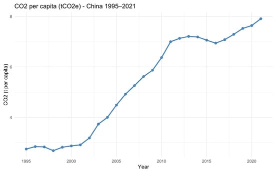
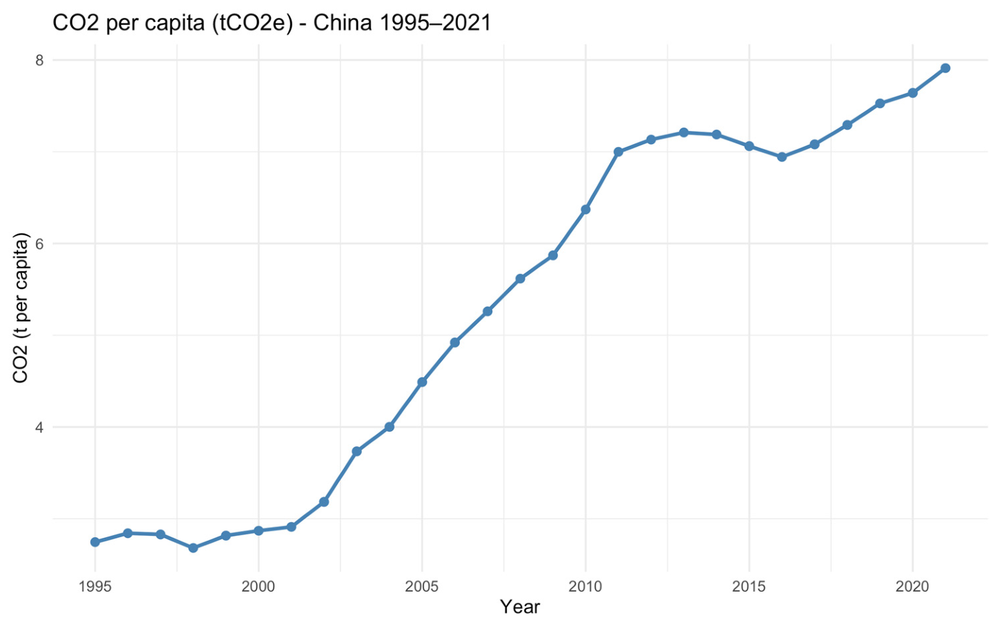
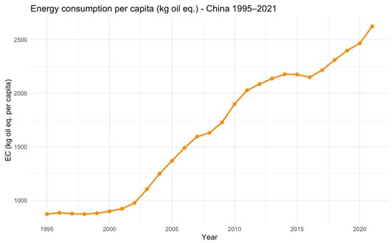
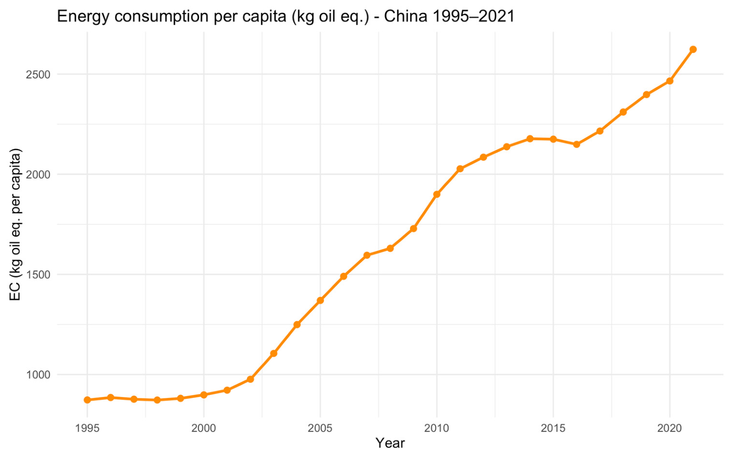
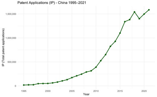
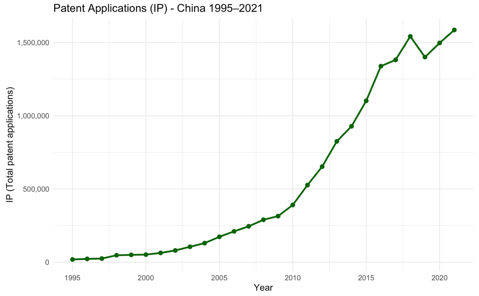
Figure 1, Figure 2 and Figure 3 show the time paths of per capita CO₂ emissions, per capita energy consumption, and total annual IP over 1995–2021. CO₂ emissions rise from the mid-1990s to a plateau around 2013, decline during 2014–2016, and increase again to their sample maximum in the final year. Energy consumption follows a broadly similar upward path, with a brief pause in the mid-2010s, and also reaches its sample maximum in the final year. IP increases approximately exponentially, with faster growth after the mid-2000s.

Figure 1. Carbon dioxide emissions per capita (metric tons) in China, 1995–2021.

Figure 2. Energy consumption per capita (kg of oil equivalent) in China, 1995–2021.

Figure 3. Total annual IP (count) in China, 1995–2021.

4.2. Fourier Unit-Root Tests

Table 3 reports the unit-root evidence. AGDP and SGDP are the only variables with clear I(0)-consistent Fourier classifications, while lnCO2, lnGDP, lnIP, IGDP, and lnGDP squared remain potentially consistent with I(2); lnEC remains unresolved because the level and differenced evidence is not jointly decisive.

Table 3. Fourier unit-root diagnostics.

Variable	ADF Level	ADF Diff1	ADF Diff2	KPSS Level [CV]	KPSS Diff1 [CV]	KPSS Diff2 [CV]	Classification
lnCO2	1.7395	−3.7108	−6.6603	0.4160 [0.346]	0.1635 [0.359]	0.1420 [0.399]	I(2) cannot be excluded
lnGDP	−0.6739	−4.5788	−5.3111	0.4314 [0.611]	0.0782 [0.327]	0.2145 [0.305]	I(2) cannot be excluded
lnEC	3.1548	−2.0166	−4.0609	0.4161 [0.338]	0.2119 [0.489]	0.1648 [0.365]	Unresolved
lnIP	−2.1268	−4.2099	−9.2387	0.4221 [0.586]	0.1819 [0.386]	0.0986 [0.269]	I(2) cannot be excluded
AGDP	−4.5912	−4.9551	−7.1486	0.4139 [0.560]	0.1608 [0.398]	0.0995 [0.258]	I(0)-consistent
IGDP	−3.4233	−3.8446	−5.7415	0.3642 [0.570]	0.1182 [0.380]	0.1820 [0.259]	I(2) cannot be excluded
SGDP	−3.9193	−3.2963	−5.1016	0.3960 [0.639]	0.0712 [0.321]	0.1423 [0.262]	I(0)-consistent
lnGDP_sq	0.2137	−4.6232	−5.5243	0.4313 [0.534]	0.0630 [0.343]	0.2106 [0.255]	I(2) cannot be excluded

These results indicate that the order of integration for the core emissions model remains uncertain.

4.3. Cointegration Test Results

Table 4 reports the bounds statistics. The overall F statistic is 7.3093, the lagged-dependent-variable t statistic is −5.1524, and the regressor-only F statistic is 9.7340.

Table 4. Bounds cointegration test with bootstrap p-values.

Statistic	Value	Bootstrap p
Overall level F	7.3093	0.1528
Lagged dependent t	−5.1524	0.9101
Regressor-only F	9.7340	0.1049

Because the integration diagnostics do not fully rule out higher-order persistence for several core variables, these statistics are informative but not sufficient on their own to establish a long-run equilibrium relationship.

The overall level F, lagged dependent t, and regressor-only F statistics are reported for completeness. Bootstrap p-values come from a restricted sieve bootstrap with 1000 replications that conditions on the regressors and the Fourier terms. The unit-root diagnostics do not establish that all variables are at most I(1): I(2) cannot be excluded for lnCO2, lnGDP, and lnIP, and lnEC is unresolved (Table 3). The integration-order pre-condition for the bounds test is therefore not satisfied, and the p-values are reported conditionally; bounds interpretation is withheld.

4.4. Classical FARDL Specification and Estimation

Table 5 reports the classical FARDL estimates for ARDL (2,1,2,1) at k = 1. The coefficient on the lagged level of emissions, lnCO2(t − 1), is −2.0149 (HAC SE = 0.5084). Crucially, as established in Section 4.3 and Table 4, bounds cointegration has not been established and the integration-order prerequisite remains unresolved. Consequently, this parameter reflects autoregressive persistence rather than error-correction adjustment toward equilibrium. Furthermore, its point estimate falls outside the standard stable interval (−1, 0), confirming the absence of a self-correcting equilibrium path. Energy consumption retains a positive and precisely estimated lagged-level coefficient (1.9924, p = 0.0029 under HAC), whereas the lagged GDP and IP coefficients are small and statistically indistinguishable from zero.

Table 5. Classical Fourier autoregressive distributed lag (FARDL) specification.

Variable	Coefficient	Std. Error	t	p
Intercept	−10.9805	2.7543	−3.9867	0.0018
lnCO2(t − 1)	−2.0149	0.5084	−3.9632	0.0019
lnGDP(t − 1)	−0.0052	0.125	−0.0415	0.9676
lnEC(t − 1)	1.9924	0.5349	3.7248	0.0029
lnIP(t − 1)	−0.0247	0.0358	−0.6895	0.5036
ΔlnGDP	−0.7699	0.4613	−1.669	0.121
ΔlnEC	1.3028	0.3044	4.2798	0.0011
ΔlnIP	−0.0171	0.0424	−0.4039	0.6934
ΔlnCO2(t − 1)	0.4385	0.279	1.5717	0.142
ΔlnEC(t − 1)	−0.4836	0.3837	−1.2601	0.2316
sin (k)	−0.0923	0.0237	−3.9036	0.0021
cos (k)	−0.0723	0.0156	−4.6391	<0.001

Note: Lagged-level variables are denoted by (t − 1) and Δ denotes first differences. The coefficient on lnCO2(t − 1) reflects autoregressive persistence rather than an error-correction mechanism, as bounds cointegration is not established. Implied lagged-level ratios represent exploratory model outputs. sin (k) and cos (k) are Fourier terms evaluated at frequency k = 1. Standard errors are HAC (Newey–West).

Evaluated as dynamic parameter ratios (−β_j/β_lnCO2,t − 1), the implied scaling for energy consumption is 0.9888, whereas the ratios for GDP (−0.0026) and IP (−0.0122) are close to zero and statistically uncertain. In the short run, contemporaneous changes in energy consumption (ΔlnEC) enter positively and strongly (1.3028, p = 0.0011 under HAC), while short-run GDP changes enter negatively (−0.7699, p = 0.121 under HAC).

Among the short-run terms, the contemporaneous change in energy consumption is strongly positive, while the GDP and IP short-run coefficients are not robustly estimated once the current specification and covariance choices are taken into account. The lagged change in CO₂ is also statistically weak, whereas the Fourier terms remain clearly non-zero.

In-sample fit is high, but the substantive interpretation rests on the coefficient pattern and the diagnostic checks rather than on goodness-of-fit statistics alone.

4.5. Lag-Order Sensitivity

Table 6 shows that the unrestricted BIC minimum occurs at ARDL (2,1,1,2), but that specification fails both Breusch–Godfrey tests at the 5% level. Among admissible models, the reference specification is ARDL (2,1,2,1) at k = 1. In the inadmissible BIC-minimum model the exploratory lagged-level IP ratio is negative and statistically different from zero under HAC inference, whereas in the admissible reference model it is small and statistically indistinguishable from zero. Across the candidate lag grid, the exploratory lagged-level ratio for energy consumption exhibits relative numerical persistence around unity, while the ratios for GDP and IP are sensitive in sign, magnitude, and precision. In the absence of established cointegration, these ratios serve strictly as exploratory model outputs capturing dynamic parameter scaling across lag orders.

Table 6. Lag-order sensitivity results.

Specification	AIC	BIC	BG1	BG2	Root	LR_GDP p	LR_EC p	LR_IP p	Status
ARDL (1,1,1,1); k = 1	−124.12	−111.17	0.1456	0.0321	0.3903	0.5453	0.0000	0.4447	Ineligible
ARDL (2,1,1,1); k = 1	−123.68	−109.54	0.1416	0.0239	0.3917	0.3586	0.0000	0.2391	Ineligible
ARDL (3,1,1,1); k = 1	−123.53	−108.21	0.3683	0.0773	0.6759	0.7084	0.0000	0.4788	Admissible
ARDL (2,2,1,1); k = 1	−122.17	−106.85	0.1618	0.0114	0.4655	0.3929	0.0000	0.2480	Ineligible
ARDL (2,1,2,1); k = 1	−126.83	−111.52	0.8856	0.1143	0.6622	0.9675	0.0000	0.5348	Reference
ARDL (2,1,1,2); k = 1	−127.88	−112.57	0.0070	0.0057	0.4803	0.0067	0.0000	0.0020	BIC minimum; fails BG

Note: ECT denotes the coefficient on lnCO2(t − 1), capturing autoregressive dynamics in the absence of cointegration. LR_columns report p-values for exploratory lagged-level coefficient ratios. BG1 and BG2 denote Breusch–Godfrey test p-values at orders 1 and 2.

4.6. Residual and Model Diagnostics

Table 7 reports the diagnostic results for the admissible reference model. The selected ARDL (2,1,2,1) specification does not reject the Breusch–Godfrey test at order two, and the remaining residual diagnostics do not indicate clear misspecification.

Table 7. Residual and model diagnostics results.

Test	Statistic	p-Value
BG(1)	0.0207	0.8856
BG(2)	4.3381	0.1143
Breusch–Pagan	12.1775	0.3505
Jarque–Bera	1.3391	0.5119
RESET(2)	1.2484	0.2877
CUSUM	0.4504	0.7391

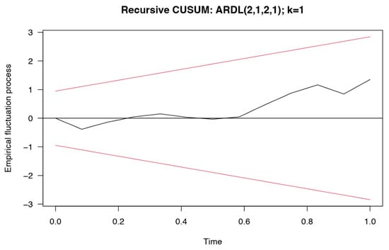
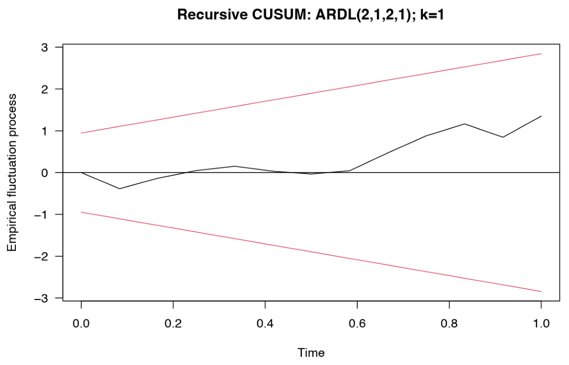
The Breusch–Pagan test does not reject homoskedasticity (p = 0.3505), the Jarque–Bera test does not reject normality (p = 0.5119), and the RESET test does not indicate functional-form misspecification (p = 0.2877). The CUSUM evidence is also consistent with parameter stability over the sample. Figure 4 shows the recursive CUSUM parameter-stability plot.

Figure 4. Recursive CUSUM parameter-stability plot. Note: The black line is the recursive CUSUM empirical fluctuation process for the reference ARDL (2,1,2,1) specification at k = 1; the red lines are the five-percent significance boundaries and time is scaled to the sample fraction. The process remains within the boundaries, consistent with parameter stability (p = 0.7391; Table 7).

4.7. EKC Test

Table 8 shows that the EKC result is specification-dependent. Because the raw correlation between lnGDP and its squared term is 0.9996, log GDP is centered before squaring; after centering, the correlation between the linear and quadratic terms falls to −0.1840. The centered-squared-income curvature is negative for k = 0, k = 2, and k = 3, but positive for the BIC-selected k = 1 specification, and the implied turning point shifts materially across Fourier frequencies.

Table 8. EKC test results.

k	BIC	Curvature	95% Interval	BG1	BG2	Turning Point
0	−107.63	−0.1284	[−0.1582, −0.0986]	0.5549	0.1229	2391
1	−125.70	0.7212	[0.0627, 1.3798]	0.0070	0.0191	4321
2	−112.62	−0.1221	[−0.1597, −0.0845]	0.0331	0.0111	2765
3	−113.60	−0.1083	[−0.1385, −0.0781]	0.0031	0.0010	1025

At k = 0, k = 2, and k = 3 the linear GDP term is positive and the squared term is negative, implying inverted-U shapes with turning points of about 2391, 2765, and 1025 constant 2015 US dollars per capita, respectively. At k = 1 the curvature turns positive, which reinforces the sensitivity of the EKC result to the Fourier specification.

Thus, the EKC exercise does not support a single stable income–emissions curve for China. The results indicate substantial sensitivity to the Fourier specification.

4.8. Recursive Expanding-Window Stability

Table 9 reports recursive expanding-window estimates. Across the windows from 1998–2019 to 1998–2021, the exploratory ratio for energy remains stable near unity (ranging from 0.9620 to 1.0219), while the ratios for GDP and IP remain close to zero. Although this pattern indicates empirical persistence in the sample correlation between lagged energy and emissions levels, it represents descriptive parameter stability within the estimated dynamic model.

Table 9. Recursive expanding-window stability results.

Window	n	ECT	LR_GDP	LR_EC
1998–2019	22	−2.3656	−0.0334	1.0219
1998–2020	23	−2.2821	−0.0156	0.9620
1998–2021	24	−2.0149	−0.0026	0.9888

Note: ECT denotes the coefficient on lnCO2(t − 1), capturing autoregressive dynamics. Columns LR_GDP and LR_EC report exploratory lagged-level coefficient ratios.

4.9. Scenario Analysis Results

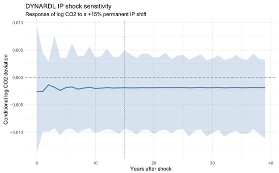
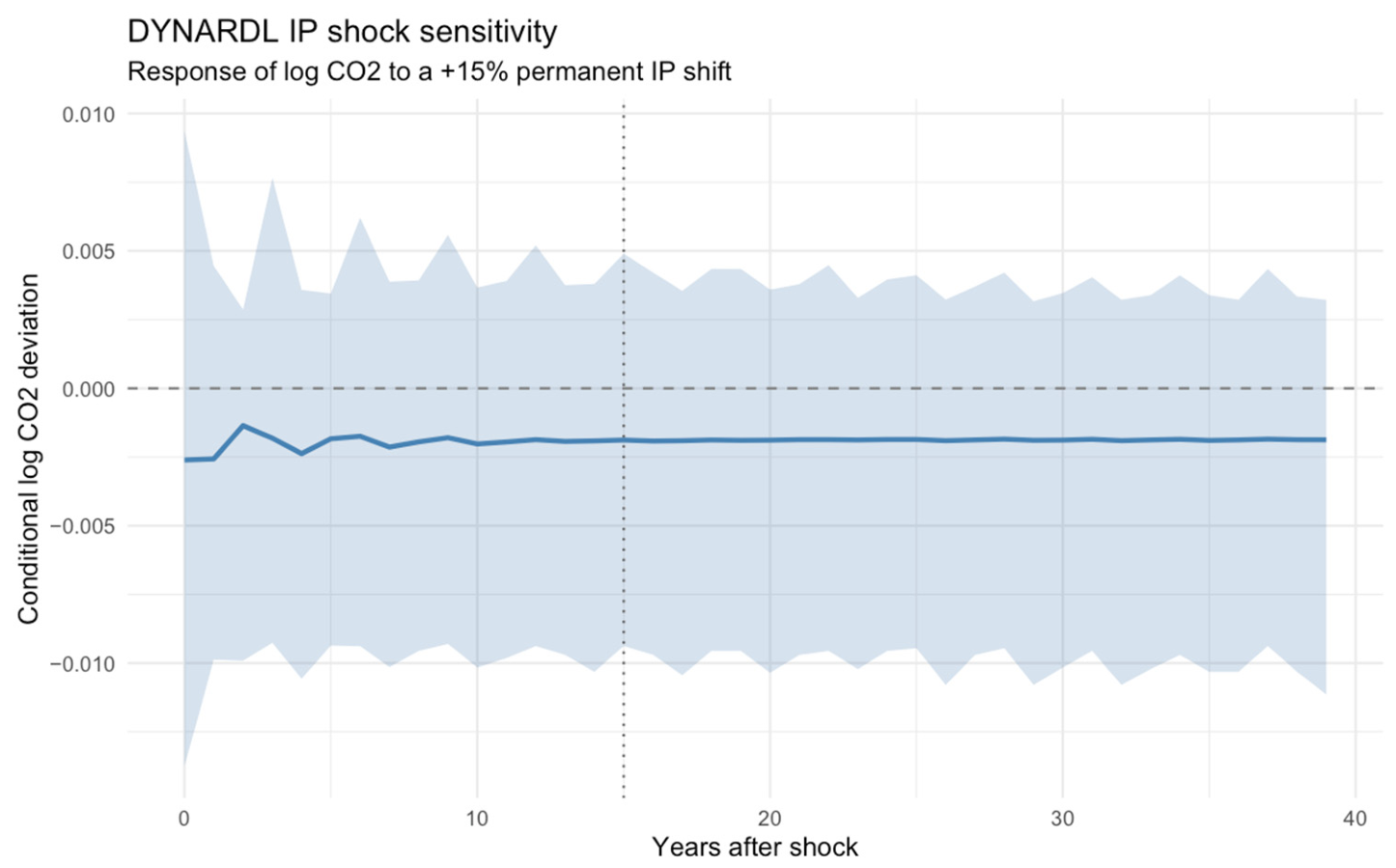
Figure 5 reports the DYNARDL sensitivity analysis for a permanent 15% IP shock under the selected ARDL (2,1,2,1) model. The median response of log CO₂ is slightly negative throughout the horizon, but the interval estimate includes zero at every point.

Figure 5. Dynamic ARDL impulse response. Note: The dotted vertical line marks the 15-period interim horizon.

At the 15-period horizon, the median response is about −0.0018, with a 95% interval from roughly −0.0094 to 0.0049. At the 40-period horizon, the median response remains close to −0.0018, with a 95% interval from about −0.0111 to 0.0032.

The simulation therefore does not support a persistent emissions-reduction effect from aggregate IP in this dynamic specification, even though the median response is mildly negative across the horizon.

4.10. Bayesian FARDL Results

Table 10 reports the Bayesian estimation of the selected reference model. The posterior mean of the lagged-dependent-variable coefficient is −1.3408, with a 95% credible interval from −2.1019 to −0.4456 (Table 10). The lagged energy coefficient remains clearly positive, whereas the lagged GDP and IP coefficients continue to span zero.

Table 10. Bayesian FARDL.

Parameter	Estimate	Est.Error	Q2.5	Q97.5
b_Intercept	−7.1195	2.3585	−11.3520	−2.0981
b_L_lnCO2	−1.3408	0.4197	−2.1019	−0.4456
b_L_lnGDP	0.0923	0.1420	−0.1805	0.3823
b_L_lnEC	1.2048	0.4635	0.2248	2.0380
b_L_lnIP	−0.0252	0.0438	−0.1107	0.0626
b_D_lnGDP	−0.4014	0.3862	−1.1070	0.4294
b_D_lnEC	1.0182	0.2513	0.4752	1.4692
b_D_lnIP	−0.0277	0.0471	−0.1212	0.0638
b_D1_lnCO2	0.1271	0.2477	−0.3904	0.5817
b_D1_lnEC	−0.0891	0.3083	−0.6525	0.5569
b_sin_k	−0.0616	0.0331	−0.1222	0.0084
b_cos_k	−0.0617	0.0169	−0.0934	−0.0263
sigma	0.0173	0.0042	0.0111	0.0277
Intercept	0.0428	0.0036	0.0356	0.0499
lprior	−15.8868	1.3247	−18.8714	−13.9243

Note: Estimates are posterior means; Est.Error is the posterior standard deviation, and Q2.5 and Q97.5 are the 2.5% and 97.5% posterior quantiles, so the interval they span is the 95% credible interval. The b_ prefix denotes regression coefficients: L_ denotes lagged levels, D_ first differences, and D1_ one-period-lagged first differences; sin_k and cos_k are the Fourier terms evaluated at frequency k = 1. sigma is the residual standard deviation, and lprior is the log prior density. The regression coefficients use Normal (0, 1) priors. Implied ratios of lagged-level coefficients represent exploratory model outputs.

The exploratory posterior coefficient ratio for energy remains positive, whereas the exploratory ratios for GDP and IP remain close to zero and span zero. This pattern is consistent with the classical results: energy exhibits a stable empirical correlation, while the innovation association is weak.

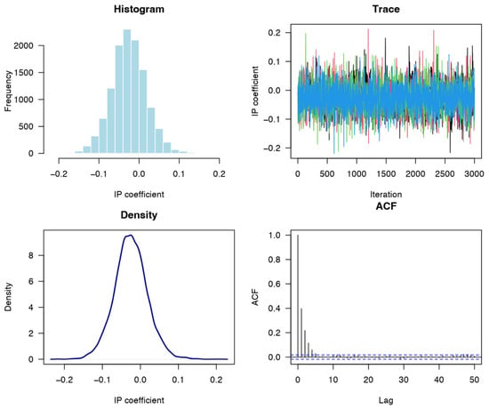
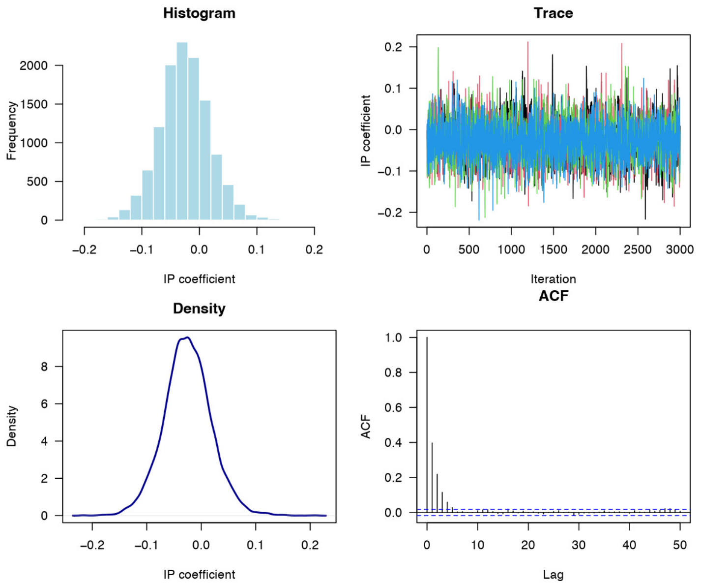
The Bayesian estimates show satisfactory convergence, with maximum R close to 1 and no divergent transitions. Figure 6 presents the posterior diagnostics for the lagged IP coefficient. The implied coefficient ratios computed from the joint posterior draws have medians of 0.9053 for energy consumption (95% credible interval: 0.4542 to 1.1193), 0.0633 for GDP (−0.1534 to 0.4496), and −0.0188 for IP (−0.1065 to 0.0707). Because bounds cointegration is not established and the integration-order prerequisite remains unconfirmed, these posterior ratios capture dynamic parameter scaling within the Bayesian ARDL framework.

Figure 6. Posterior diagnostic for the lagged log IP coefficient. Note: In the trace plot (top right), the four colors (black, red, green, and blue) denote the four independent MCMC chains. In the autocorrelation function (ACF) plot (bottom right), the horizontal blue dashed lines indicate the 95% confidence intervals for zero autocorrelation. The light blue bars (top left) and solid dark blue line (bottom left) depict the posterior frequency distribution and estimated kernel density, respectively.

4.11. Prior Sensitivity

Table 11 shows that prior sensitivity matters mainly through the denominator of the exploratory ratios. Under the diffuse Normal (0,10) prior, the lagged-level emissions coefficient remains negative and the exploratory energy ratio stays close to one. Under the tight Normal (0,0.25) prior, however, the denominator interval crosses zero and the ratio-based exploratory outputs become highly unstable.

Table 11. Prior sensitivity and denominator diagnostics.

Prior	β [95% CrI]	Pr(β < 0)	Pr(|β| < 0.10)	LR_GDP [95% CrI]	LR_EC [95% CrI]	LR_IP [95% CrI]
Baseline Normal(0,1)	−1.364 [−2.102, −0.446]	0.997	0.003	0.063 [−0.153, 0.450]	0.905 [0.454, 1.119]	−0.019 [−0.107, 0.071]
Diffuse Normal(0,10)	−1.998 [−2.887, −1.099]	1.000	0.000	−0.000 [−0.143, 0.179]	0.985 [0.793, 1.131]	−0.013 [−0.061, 0.033]
Tight Normal(0,0.25)	−0.265 [−0.622, 0.097]	0.925	0.162	0.449 [−2.670, 4.742]	0.199 [−6.207, 5.133]	0.056 [−1.287, 1.752]

Note: Posterior medians; 95% credible intervals in brackets. Probabilities are estimated from posterior draws.

For the tight prior, the posterior probability that the lagged-dependent-variable coefficient lies within 0.10 of zero rises materially, and the implied exploratory ratios become excessively wide and weakly identified. This exploratory ratio shows higher dispersion under this prior than under the baseline or diffuse priors, illustrating the mathematical sensitivity of ratio-based quantities when the denominator distribution encompasses zero in the absence of cointegration.

The baseline and diffuse priors deliver broadly similar substantive conclusions, whereas the tight prior shows how sensitive ratio-based exploratory model outputs can become when the denominator approaches zero.

4.12. Granger Causality Results

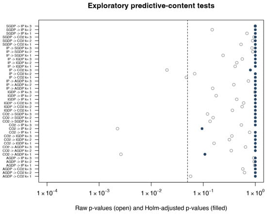
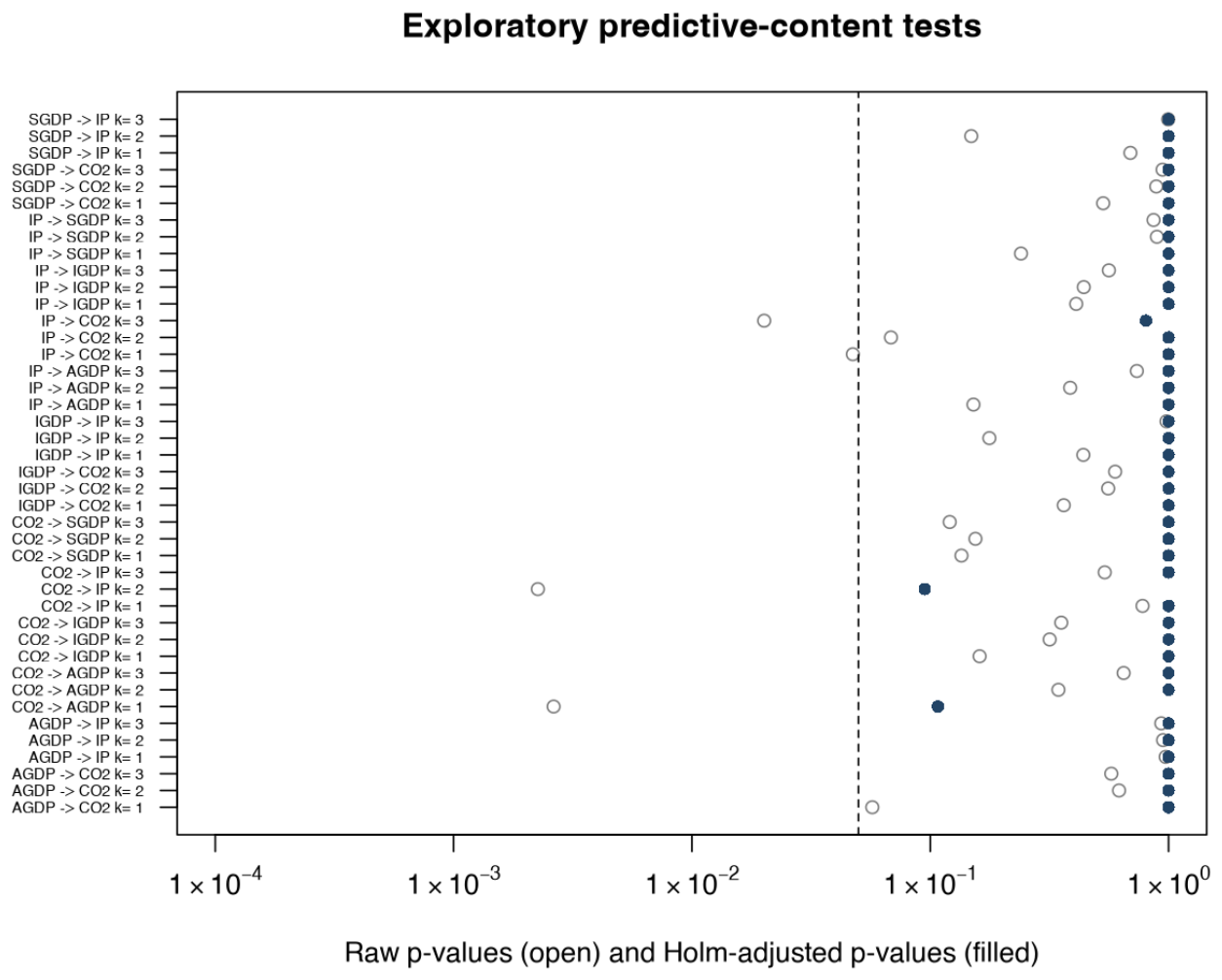
Table 12 reports the causality results. In the time domain at k = 1, CO₂ -> AGDP and IP -> CO₂ are the only directions with raw p-values below 0.05, but neither remains significant after the Holm adjustment within the time-domain family.

Table 12. Granger causality test results.

Direction	Lags	n	F	Raw p	Holm p	BG1	BG2	Note
AGDP -> CO2	1	25	4.075	0.0571	1.0000	0.0988	0.0951	Exploratory
CO2 -> AGDP	2	24	8.600	0.0026	0.1078	0.4388	0.6895	Exploratory
AGDP -> IP	3	23	0.075	0.9725	1.0000	0.2746	0.3098	Exploratory
IP -> AGDP	2	24	2.110	0.1518	1.0000	0.4228	0.1476	Exploratory
IGDP -> CO2	1	25	0.865	0.3633	1.0000	0.6548	0.8976	Exploratory
CO2 -> IGDP	3	23	1.995	0.1612	1.0000	0.7369	0.8464	Exploratory
IGDP -> IP	3	23	0.960	0.4389	1.0000	0.9125	0.4943	Exploratory
IP -> IGDP	3	23	1.029	0.4097	1.0000	0.0223	0.0393	Exploratory
SGDP -> CO2	1	25	0.405	0.5317	1.0000	0.0926	0.2422	Exploratory
CO2 -> SGDP	3	23	2.185	0.1352	1.0000	0.5469	0.2611	Exploratory
SGDP -> IP	3	23	0.495	0.6916	1.0000	0.8053	0.5590	Exploratory
IP -> SGDP	3	23	1.572	0.2403	1.0000	0.0021	0.0039	Exploratory
IP -> CO2	3	23	3.412	0.0473	1.0000	0.0305	0.0924	Exploratory
CO2 -> IP	3	23	0.367	0.7778	1.0000	0.5372	0.3852	Exploratory

In the frequency domain, CO₂ -> AGDP at k = 1 is the clearest signal, with raw p-values of about 0.0002 across the reported frequencies and Holm-adjusted p-values of about 0.0227 within the spectral family and 0.0460 across all reported tests. IP -> CO₂ also records lower raw p-values at omega = 0.5, 1.0, and 1.5, but these do not survive multiplicity adjustment.

Most other directions are weak or inconsistent. CO₂ -> IGDP and CO₂ -> SGDP show some lower raw p-values at the lowest frequencies, and CO₂ -> IP becomes small only at k = 2 in the time domain, but these patterns are not stable across the reported specifications. Figure 7 shows exploratory predictive-content tests.

Figure 7. Exploratory predictive-content tests. Note: Open circles show raw p-values and filled circles show p-values adjusted by the Holm procedure within the family of time-domain directional tests. The dashed vertical line marks the five percent level; the horizontal axis is on the log scale.

4.13. Fourier Frequency Sensitivity

Table 13 shows that the time-domain results are sensitive to the deterministic Fourier frequency. For example, the IP -> CO₂ raw p-value is 0.0473 at k = 1, 0.0684 at k = 2, and 0.0201 at k = 3, while CO₂ -> IP is insignificant at k = 1 and k = 3 but falls to 0.0023 at k = 2.

Table 13. Robustness. Panel A: FARDL estimates; Panel B: Time-Domain Granger Causality bootstrap p-values; Panel C: Breitung–Candelon bootstrap p-values by frequency.

(A)
k		BIC	LR_GDP	LR_EC	LR_IP	ECT
0		−82.87	−0.7524	1.4496	0.0914	−0.0662
1		−111.52	−0.0026	0.9888	−0.0122	−2.0149
2		−79.24	−275.1890	−1079.3094	436.4276	−0.0005
3		−87.91	−1.1587	1.6520	0.3354	−0.6482
(B)
Direction		k = 1	k = 2	k = 3
AGDP -> CO2		0.0571	0.6198	0.5750
CO2 -> AGDP		0.0026	0.3451	0.6480
AGDP -> IP		0.9725	0.9484	0.9320
IP -> AGDP		0.1518	0.3866	0.7362
IGDP -> CO2		0.3633	0.5580	0.5969
CO2 -> IGDP		0.1612	0.3170	0.3547
IGDP -> IP		0.4389	0.1770	0.9806
IP -> IGDP		0.4097	0.4408	0.5618
SGDP -> CO2		0.5317	0.8882	0.9436
CO2 -> SGDP		0.1352	0.1547	0.1207
SGDP -> IP		0.6916	0.1486	0.9966
IP -> SGDP		0.2403	0.8936	0.8652
IP -> CO2		0.0473	0.0684	0.0201
CO2 -> IP		0.7778	0.0023	0.5397
(C)
Direction	k	ω = 0.5	ω = 1.0	ω = 1.5	ω = 2.0	ω = 2.5
CO2 -> AGDP	1	0.0002	0.0002	0.0002	0.0002	0.0002
CO2 -> AGDP	2	0.1739	0.1658	0.1670	0.1707	0.1723
CO2 -> AGDP	3	0.4303	0.4632	0.5580	0.5807	0.5815
IP -> CO2	1	0.0084	0.0063	0.0104	0.0911	0.1487
IP -> CO2	2	NA	NA	NA	NA	NA
IP -> CO2	3	NA	NA	NA	NA	NA
CO2 -> IP	1	0.7577	0.8804	0.8911	0.6935	0.6297
CO2 -> IP	2	0.0000	0.0000	0.0623	0.8212	0.9918
CO2 -> IP	3	0.3250	0.4007	0.7548	0.9382	0.9670

Note: Panels B and C report p-values from the F test of no Granger causality and from the Breitung–Candelon chi-squared test across frequencies, respectively. Statistical significance is assessed at the 5% level (p < 0.05); values between 0.05 and 0.10 indicate weak significance. NA indicates that the Breitung–Candelon test is not reported because the AIC lag order is one. In Panel A, entries in the LR columns are exploratory lagged-level coefficient ratios, and ECT reports the autoregressive coefficient on lnCO2(t − 1).

More generally, the CO₂ -> AGDP signal is concentrated at k = 1, whereas the reverse CO₂ -> IP signal appears only at k = 2. None of these time-domain findings survives the Holm adjustment across the full time-domain family, which underscores their sensitivity to the deterministic Fourier specification. The causality results therefore establish frequency-sensitive short-run predictive associations in first differences, reflecting localized dynamic interactions without long-run equilibrium feedback.

4.14. Discussion

China’s emissions trajectory is driven by immediate, physical energy throughput in first differences, operating independently of an autonomous error-correcting equilibrium path. While economic growth, technological innovation, and sectoral restructuring are widely hypothesized as structural forces capable of decoupling emissions from output, our results demonstrate that aggregate carbon emissions remain tightly coupled to contemporaneous energy consumption in first differences. In contrast, neither an Environmental Kuznets Curve (EKC) nor a long-run innovation decoupling mechanism is empirically substantiated once smooth structural breaks and integration-order constraints are rigorously accounted for.

The study found that long-run cointegration among output, energy, and emissions cannot be established. When subjected to flexible Fourier unit-root diagnostics, higher-order persistence (I(2)) cannot be ruled out for emissions, output, and innovation, while the integration order for energy consumption remains ambiguous. Failure to satisfy this foundational prerequisite formally precludes bounds cointegration inference. Furthermore, the autoregressive level parameter on emissions falls outside the theoretical stability interval of (−1, 0), demonstrating the absence of an empirical error-correction mechanism. These findings demonstrate that apparent cointegrating equilibrium vectors in aggregate time series can arise as statistical anomalies when integration-order prerequisites are left unverified.

The physical and institutional structure of the Chinese economy explains why contemporaneous differenced energy use dominates in the absence of long-run equilibrium adjustment. China’s growth model over 1995–2021 was heavily anchored in carbon-intensive capital stock, heavy industrial manufacturing, and coal-fired power generation. Annual fluctuations in industrial output translate directly and immediately into energy throughput, which generates carbon emissions contemporaneously in physical lockstep. Lacking an automatic market-clearing equilibrium to restore a steady-state emissions path, emissions mechanically follow physical energy utilization.

Our empirical findings also indicate that technological innovation does not serve as an automatic aggregate carbon mitigator in this aggregate setting. The aggregate innovation indicator yields an implied lagged-level ratio statistically indistinguishable from zero, with dynamic simulations spanning zero across all forecast horizons. This pattern reflects the composition of aggregate patent filings in China, which are heavily weighted toward utility models and production-oriented industrial patents that can expand production capacity and induce energy rebound effects rather than reduce carbon intensity. Similarly, the quadratic income relationship proves fragile and sensitive to Fourier frequencies, confirming that income growth alone does not generate an autonomous, inverted-U turning point for China’s aggregate emissions. The bivariate causality results indicate that sectoral output shares (AGDP, IGDP, SGDP) display frequency-specific predictive content with respect to differenced emissions, but these relationships do not survive multiple-testing adjustments across frequencies. Because the sectoral shares are compositionally constrained and evaluated outside a cointegrated level system, sectoral reallocation over 1995–2021 has not functioned as an independent, exogenous decarbonization mechanism separate from overall energy intensity.

These findings establish an essential methodological principle for applied environmental econometrics: verifying integration-order prerequisites is mandatory before interpreting lagged-level coefficient ratios. Without confirmed cointegration, interpreting such ratios as structural policy elasticities generates unsupported parameters. The Bayesian prior-sensitivity analysis reinforces this point: under tighter priors, the denominator of the ratio spans zero, causing the implied elasticity to diverge dramatically. Parameter ratios within an ARDL specification capture dynamic parameter scaling, not structural long-run cointegrating multipliers, unless cointegration is formally established.

For policymakers, this analysis demonstrates that market forces cannot be assumed to steer China toward an emissions peak via autonomous error correction or natural EKC maturation. Because emissions respond contemporaneously to annual energy throughput, decarbonization cannot rely on passive economic growth or unguided aggregate innovation. Instead, achieving China’s 2030 peaking and 2060 neutrality targets requires direct, proactive structural interventions: enforceable absolute caps on fossil energy consumption, accelerated electrification of heavy industry with non-fossil power, and targeted deployment of zero-carbon technologies. This underscores that achieving genuine ecological balance requires active governance of aggregate energy throughput rather than reliance on market-driven efficiency gains.

This study evaluated aggregate national annual dynamics over 1995–2021 (T = 27). The presence of unresolved integration orders formally bounds the scope of cointegration inference, while aggregate patent filings encompass both green and general industrial technologies. Within these analytical boundaries, the empirical findings remain decisive. By deploying a coordinated multi-track strategy combining classical Fourier ARDL, Bayesian NUTS estimation, prior-sensitivity analysis, and spectral Granger causality, we show that contemporaneous energy–emissions coupling is robust across all specifications and priors, while steady-state cointegration is consistently absent.

These findings establish a clear agenda for subsequent research. Future empirical investigations of China’s aggregate emissions should implement fractional cointegration frameworks and multivariate models specifically designed to handle potential I(2) persistence. Furthermore, compiling disaggregated provincial and enterprise-level panel datasets will be essential to track how targeted green patent diffusion and industrial sub-sector restructuring impact carbon intensity directly. Ultimately, China’s carbon emissions trajectory is not an autonomous equilibrium process governed by automatic market reversion, but a physical reality dictated by immediate energy throughput, demanding deliberate, structural transformation over passive assumptions of statistical equilibria.

5. Conclusions

This study examined China’s carbon mitigation dynamics over the 1995–2021 industrial expansion period, evaluating carbon dioxide emissions alongside energy consumption, economic growth, and technological innovation within Fourier and Bayesian Fourier ARDL specifications, while assessing sectoral structural shares through dedicated predictive-content tests. Crucially, the empirical evidence demonstrates that aggregate emissions and energy use do not form a cointegrated relationship. Unresolved integration-order properties invalidate the foundational prerequisite for ARDL bounds testing, formally precluding cointegration inference. Consequently, bounds-test interpretation is withheld, establishing that the data do not support a cointegrating equilibrium.

Empirically, China’s carbon emissions trajectory does not track toward an internal, self-correcting steady-state economic balance. Instead, annual emissions are determined primarily by contemporaneous physical industrial energy throughput in first differences. In the absence of cointegration, the near-unity lagged-level coefficient ratios obtained across classical OLS and Bayesian estimations reflect dynamic parameter scaling within the estimated specification rather than equilibrium elasticities. Furthermore, aggregate patent applications exhibit no statistically discernible emissions-mitigation effect, and the Environmental Kuznets Curve demonstrates sign-switching instability across Fourier frequencies. Without an automatic error-correction mechanism pulling emissions toward an equilibrium path, mitigation policy cannot rely on unverified steady-state dynamics or passive market-driven turning points. The absence of cointegration reinforces the necessity of direct, structural decarbonization of the energy mix. With annual emissions tethered directly to real-time energy throughput, achieving China’s 2030 peaking and 2060 carbon neutrality targets requires proactive, real-time intervention: establishing enforceable absolute caps on fossil energy consumption, accelerating zero-carbon electrification across industrial sectors, and directly substituting coal with renewable power. Ultimately, sustainable development in an energy-intensive economy cannot be treated as an automatic outcome of economic expansion, but depends on decisive institutional interventions to curb fossil reliance.

Methodologically, these findings demonstrate the necessity of strict diagnostic gating in environmental time-series econometrics. Without verifying integration-order prerequisites, aggregate ARDL regressions risk mistaking transient autoregressive persistence for structural equilibrium cointegration. Establishing these diagnostic boundaries ensures that climate policy is grounded directly in verified empirical reality.

References

- Gao, W.; Wang, M.; Ye, T. Is China’s carbon neutrality commitment truly credible? Evidence from a natural experiment. Financ. Res. Lett. 2022, 50, 103284. [Google Scholar] [CrossRef] [Scilit]
- Nurgazina, Z.; Guo, Q.; Ali, U.; Kartal, M.T.; Ullah, A.; Khan, Z.A. Retesting the Influences on CO2 Emissions in China: Evidence From Dynamic ARDL Approach. Front. Environ. Sci. 2022, 10, 868740. [Google Scholar] [CrossRef] [Scilit]
- Zhao, H.; Hu, J.; Hao, F.; Zhang, H. Determinants of Carbon Dioxide Emissions and Their Peaking Prospect: Evidence From China. Front. Environ. Sci. 2022, 10, 913835. [Google Scholar] [CrossRef] [Scilit]
- Jin, H.; Liu, L.; Sun, X. Research on the scenario prediction and classification of emission reduction strategy of carbon emission in china’s oil and gas industry. Energy Rep. 2025, 14, 2264–2279. [Google Scholar] [CrossRef] [Scilit]
- Yan, J.; Lu, W.; Xu, X.; Lian, J. Empirical Study of the Environmental Kuznets Curve in China Based on Provincial Panel Data. Sustainability 2023, 15, 5225. [Google Scholar] [CrossRef] [Scilit]
- Sikder, M.; Wang, C.; Yao, X.; Huai, X.; Wu, L.; KwameYeboah, F.; Wood, J.; Zhao, Y.; Dou, X. The integrated impact of GDP growth, industrialization, energy use, and urbanization on CO2 emissions in developing countries: Evidence from the panel ARDL approach. Sci. Total Environ. 2022, 837, 155795. [Google Scholar] [CrossRef] [Scilit] [PubMed]
- Li, W.; Elheddad, M.; Doytch, N. The impact of innovation on environmental quality: Evidence for the non-linear relationship of patents and CO2 emissions in China. J. Environ. Manag. 2021, 292, 112781. [Google Scholar] [CrossRef] [Scilit] [PubMed]
- Agan Celik, B. Driving Sustainable Development Through Sectoral Innovation Patents: The Case of Agriculture, Energy, Industry, and Transportation in China. Energy Res. Lett. 2026, 7, 160276. [Google Scholar] [CrossRef] [Scilit]
- Huang, X.; Wu, X.; Guo, X.; Shen, Y. Agricultural carbon emissions in China: Measurement, spatiotemporal evolution, and influencing factors analysis. Front. Environ. Sci. 2024, 12, 1488047. [Google Scholar] [CrossRef] [Scilit]
- Wang, D.H.; Hussain, R.Y.; Ahmad, I. Nexus between agriculture productivity and carbon emissions a moderating role of transportation; evidence from China. Front. Environ. Sci. 2023, 10, 1065000. [Google Scholar] [CrossRef] [Scilit]
- Wu, C.F.; Chang, T.; Wu, T.P.; Leng, K.J.; Lin, M.C.; Huang, S.C. Impact of globalization on the environment in major CO2-emitting countries: Evidence using bootstrap ARDL with a Fourier function. Front. Public Health 2022, 10, 907403. [Google Scholar] [CrossRef] [Scilit] [PubMed]
- Ersin, Ö.Ö. Decoupling of CO2 Emissions from Growth with Energy Transition and Eco-Innovations in OECD: Novel Fourier-CS-ARDL and Fourier-DH-Causality Analyses. Sustainability 2026, 18, 2728. [Google Scholar] [CrossRef] [Scilit]
- McNown, R.; Sam, C.Y.; Goh, S.K. Bootstrapping the autoregressive distributed lag test for cointegration. Appl. Econ. 2018, 50, 1509–1521. [Google Scholar] [CrossRef] [Scilit]
- Gong, Y.; Cao, H.; Yuan, L. Does patent pledge reduce pollution and carbon emissions? Evidence from China. Environ. Res. 2024, 247, 118274. [Google Scholar] [CrossRef] [Scilit] [PubMed]
- Liu, J.; Kang, S.J. The Impact of Green Innovation on CO2 Emissions in China: Evidence from Spatial Regression Model. Int. Econ. J. 2024, 38, 446–470. [Google Scholar] [CrossRef] [Scilit]
- Wen, Y.; Zheng, L.; Gu, Y.; Yang, X. Impacts of green technology innovation on carbon emissions: A spatial-based perspective. Technol. Anal. Strateg. Manag. 2025, 37, 4127–4139. [Google Scholar] [CrossRef] [Scilit]
- Shan, H.; Shao, S. Impact of green innovation on carbon reduction in China. Sci. Rep. 2024, 14, 14032. [Google Scholar] [CrossRef] [Scilit] [PubMed]
- Li, Q. Revisiting the determinants of CO2 emissions: The role of higher education under the extended STIRPAT model. PLoS ONE 2025, 20, e0319930. [Google Scholar] [CrossRef] [Scilit] [PubMed]
- Raihan, A.; Voumik, L.C.; Mohajan, B.; Rahman, M.S.; Zaman, M.R. Economy-energy-environment nexus: The potential of agricultural value-added toward achieving China’s dream of carbon neutrality. Carbon Res. 2023, 2, 43. [Google Scholar] [CrossRef] [Scilit]
- Kim Chung, D.T.; Xuan, V.N.; Hoa, P.X. Asymmetric roles of innovation and renewable energy in shaping carbon emissions in China. Environ. Sustain. Indic. 2026, 30, 101145. [Google Scholar] [CrossRef] [Scilit]
- Gurbuz, E.C. The impacts of economic growth, foreign direct investment inflows, and energy usage on air pollution through globalization in China: A vector error correction model approach. Energy Environ. 2026, 37, 511–539. [Google Scholar] [CrossRef] [Scilit]
- Sun, W.; Huo, Z.; Zhang, S. Dissertation title: Decoupling analysis of building carbon emissions and economic growth based on Tapio model and EKC curve. Carbon Balance Manag. 2025, 20, 63. [Google Scholar] [CrossRef] [Scilit] [PubMed]
- Atasever, G. The Interconnections among Carbon Emissions, Economic Growth, Tourism, and Energy Use in China: Testing the EKC Hypothesis Through the ARDL Approach. Ekoist J. Econom. Stat. 2026, 44, 178–194. [Google Scholar] [CrossRef] [Scilit]
- Lian, W.; Zhao, X.; Wang, J.; Duan, H.; Gao, T.; Sun, X. Renewable energy utilization and regional carbon emission reduction: Exploring nonlinear spatial spillover effects. Clean Technol. Environ. Policy 2026, 28, 53. [Google Scholar] [CrossRef] [Scilit]
- Sohaib, M.; Majeed, A.; Liu, J.; Oláh, J. The role of renewable energy in mitigating carbon emissions: Insights from China’s energy consumption patterns. Energy Strategy Rev. 2025, 61, 101860. [Google Scholar] [CrossRef] [Scilit]
- Hu, Y.; Guan, K.; Wang, S. Challenging the Environmental Kuznets Curve in China: Evidence from a dynamic panel threshold model with cross-sectional dependence. J. Environ. Manag. 2026, 398, 128432. [Google Scholar] [CrossRef] [Scilit] [PubMed]
- Mohammed, K.S.; Magdalena, R.; Alofaysan, H.; Hagiu, A. The Impact of Green and Energy Investments on Environmental Sustainability in China: A Technological and Financial Development Perspectives. Environ. Model. Assess. 2025, 30, 1147–1167. [Google Scholar] [CrossRef] [Scilit]
- Amer, E.A.A.A.; Xiuwu, Z.; Linlu, H.; Hongyuan, C.; Meyad, E.M.A.; Abdelwahed, A. When coal meets growth: Exploring the interactive impact of energy use and economic expansion on China’s carbon emissions. Results Eng. 2026, 31, 111486. [Google Scholar] [CrossRef] [Scilit]
- Yuan, Z.; Wu, R.; Fang, W.; Liu, Y. Analysis of the spatiotemporal evolution and drivers of agricultural carbon emissions: Evidence from provincial-level regions of China. Sci. Rep. 2026, 16, 925. [Google Scholar] [CrossRef] [Scilit] [PubMed]
- Koondhar, M.A.; Wang, J.J.; Ahmed, S.; Khan, Z.A. Structural change in agricultural inputs and greenhouse gas Emissions: Pathways for sustainable environmental management in China. J. Environ. Manag. 2026, 399, 128628. [Google Scholar] [CrossRef] [Scilit] [PubMed]
- Wang, Y.; Wang, W.; Wang, Z.; Yu, P.; Deng, X. Exploring the synergy between grain productivity growth and greenhouse gas emission reduction in China. Humanit. Soc. Sci. Commun. 2026, 13, 921. [Google Scholar] [CrossRef] [Scilit]
- Han, F.; Feng, J.; Abbas, A. Research on multi-scenario prediction and differentiated emission reduction strategies for China’s agricultural carbon peaking based on the XGBoost learning machine algorithm. Front. Environ. Sci. 2026, 14, 1761598. [Google Scholar] [CrossRef] [Scilit]
- Hang, Y.; Wang, Q.; Zhou, D.; Zhang, L. Factors influencing the progress in decoupling economic growth from carbon dioxide emissions in China’s manufacturing industry. Resour. Conserv. Recycl. 2019, 146, 77–88. [Google Scholar] [CrossRef] [Scilit]
- Pesaran, M.H.; Shin, Y.; Smith, R.J. Bounds testing approaches to the analysis of level relationships. J. Appl. Econom. 2001, 16, 289–326. [Google Scholar] [CrossRef] [Scilit]
- Narayan, P.K. The saving and investment nexus for China: Evidence from cointegration tests. Appl. Econ. 2005, 37, 1979–1990. [Google Scholar] [CrossRef] [Scilit]
- Vehtari, A.; Simpson, D.; Gelman, A.; Yao, Y.; Gabry, J. Pareto Smoothed Importance Sampling. J. Mach. Learn. Res. 2024, 25, 1–58. [Google Scholar]
Disclaimer/Publisher’s Note: The statements, opinions and data contained in all publications are solely those of the individual author(s) and contributor(s) and not of MDPI and/or the editor(s). MDPI and/or the editor(s) disclaim responsibility for any injury to people or property resulting from any ideas, methods, instructions or products referred to in the content. |
© 2026 by the authors. Licensee MDPI, Basel, Switzerland. This article is an open access article distributed under the terms and conditions of the Creative Commons Attribution (CC BY) license.