


Abstract
Distribution flexibility can be overvalued when priced before network-side alternatives and resource deliverability are screened. This study develops a three-gate appraisal framework for local flexibility as a non-wires alternative (NWA): network incrementality, resource deliverability, and conditional economic value. The framework is demonstrated on the IEEE 33-bus benchmark using the observed Lithuanian 2025 hourly load shape and the 2026 Energy Distribution Operator (DSO) flexibility product as well as the Lithuanian National Energy Regulatory Council (VERT) context; it is not an actual Lithuanian feeder model. At the year-3 stress point, the normal topology violates the 0.95 p.u. analytical threshold, but the screened connected-radial topology space contains a compliant configuration, so paid flexibility has no incremental value in that benchmark state if an equivalent configuration is operationally permissible. In contrast, the Zone-C L22 contingency remains non-compliant after topology-only screening and leaves a 222.1 kW local residual requirement at buses 23–24. With a 20% controllable-demand bound, 106.1 kW of firm injection remains necessary, showing that an electrical support requirement may map to demand response, firm injection, or a hybrid portfolio. Economic eligibility then depends on the genuinely deferrable share of reinforcement. The contribution is the ordered stopping logic that separates electrical need, physical deliverability, and attributable economic value.
1. Introduction
Electricity distribution networks are moving from a largely passive infrastructure role toward active coordination of distributed generation, storage, electric vehicles, heat pumps and responsive demand. This shift creates a planning problem that is both technical and economic: local constraints may arise for only a limited number of hours, while traditional reinforcement creates capacity for decades. Demand and distributed-energy-resource (DER) flexibility can therefore have value beyond short-term energy balancing when it avoids or postpones network investment, increases utilisation of existing assets and accelerates the connection of new low-carbon resources [1,2]. The policy direction is explicit in the European Union. Article 32 of Directive (EU) 2019/944 requires distribution system operators (DSOs) to consider market-based flexibility where it can reduce the need to upgrade or replace electricity capacity [3], and the Agency for the Cooperation of Energy Regulators (ACER) 2025 methodology formalises the assessment of national flexibility needs [4].
The planning interpretation of flexibility is more demanding than the trading interpretation. A market platform may record, for example, a bid of 100 kW for two hours. A network planner must also determine whether the service is electrically effective at the constrained location, whether a lower-cost network action such as reconfiguration already removes the constraint, whether the asset can sustain the requested power for the required duration, and whether the service remains preferable to the investment it is intended to defer. Ignoring any of these conditions can overstate the non-wires alternative (NWA) value attributable to flexibility. This issue is especially important when flexibility is used as a synonym for demand reduction. In distribution planning, flexibility may be delivered through reduced or shifted consumption, battery discharge, controllable generation, curtailed export, reactive-power control, or combinations of these resources; the feasible technology set depends on the sign, location, timing, and duration of the network need [5,6,7,8,9].
Lithuania is a useful institutional case because the market architecture is moving from general flexibility principles to a concrete DSO procurement framework. The IEA’s Lithuania 2025 review identifies demand-side flexibility and aggregation as important enablers of continued electrification [10]. AB Energijos skirstymo operatorius (ESO) currently defines flexibility as active adjustment of electricity consumption and/or generation in response to distribution-network needs and requires providers to bid separately for defined network locations [11]. The approved long-term active-power product remunerates availability and activation, permits aggregation, uses 1 kW granularity, specifies 15–60 min activation, allows delivery periods from 60 min to 12 h, requires 24 h recovery and requires 100% availability for the contracted product [11]. The 2026 trading rules of the Lithuanian National Energy Regulatory Council (VERT) further require the economic assessment to be performed for each network section separately and link the maximum procurement expenditure to the reconstruction cost and the number of years by which reconstruction is deferred [12].
1.1. Flexibility as a Network-Planning Resource
The economic case for a flexibility-based NWA is counterfactual. The relevant question is not whether flexibility has an intrinsic price, but what cost, timing and network performance would occur without it. Pudjianto et al. [13] showed early that active demand management can reduce distribution reinforcement driven by electrification. Later reviews of distribution system expansion planning emphasised that DERs, active network management and new market designs require planning models that integrate operational and investment decisions rather than treating flexibility as an exogenous benefit [14,15]. Lustenberger et al. [16] linked local-flexibility-market price feedback to distribution planning and demonstrated that network reinforcement can be delayed when flexibility is available at an economically attractive price.
Recent work has sharpened this counterfactual logic. Messias et al. [5] model distributed flexibility as virtual capacity and explicitly value it against conventional network projects. Their subsequent welfare-oriented procurement framework shows that a DSO’s valuation threshold and market-clearing outcome are related but distinct concepts [17]. Park and Joo [6] demonstrate that NWA portfolios combining storage with PV or demand response can materially change the required storage capacity across load profiles. García-Santacruz et al. [7] go further by separating the identification of the technical network-support need from the subsequent economic selection and sizing of generation and storage technologies. These studies make one point clear: a technically specified flexibility requirement is not yet an implementable NWA project.
1.2. Topology, Location and Incrementality
The value of flexibility is strongly location-dependent because an equal active-power change at two nodes can have different effects on branch flows and bus voltages. Mehinovic et al. [18,19] quantify this location effect and incorporate it into local flexibility-market clearing. This locational dependence becomes more complex when the DSO can reconfigure the network. Valarezo et al. [20] jointly optimise network investment, distribution network reconfiguration (DNR) and third-party flexibility, showing that reconfiguration alone may suffice under moderate demand growth and that topology changes can alter which flexibility service providers (FSPs) are eligible or effective. A 2026 follow-up explicitly coordinates DNR and local flexibility markets under alternative governance arrangements [21]. Therefore, assigning monetary value to flexibility while holding an avoidably suboptimal topology fixed can overstate its incremental value.
This observation is particularly relevant to the IEEE 33-bus benchmark, which is frequently presented as a radial feeder but includes five normally open tie branches. The standard branch-status representation enables alternative radial configurations, and recent reconfiguration studies continue to reproduce the well-known loss-reducing open-switch set 7, 9, 14, 32 and 37 [22]. A defensible NWA study using this benchmark should therefore screen reconfiguration before monetising a flexibility requirement. The purpose of such a screen is not to claim that switching is always free or operationally admissible; protection coordination, switching limits, fault-level constraints and reliability criteria can prohibit a technically feasible topology. Rather, the burden of proof is reversed: paid flexibility is incremental only after lower-cost operational alternatives are shown to be unavailable or insufficient.
Normal-state reconfiguration is only part of the planning problem. After a branch outage, service restoration requires a new radial topology that excludes the failed element while maintaining connectivity and acceptable operating conditions. Recent studies treat post-fault DNR as a self-healing or resilience action and explicitly evaluate voltage, load restoration and radiality under contingency states [23,24]. This literature motivates a broader screening rule for NWA valuation: a paid flexibility requirement should be evaluated only after the connected-radial electrical candidate space has been exhausted, rather than after one arbitrarily selected tie-switch action.
1.3. Physical Deliverability: Demand Response Is Not Unlimited Flexibility
A second weakness in simplified flexibility models is the absence of resource-level feasibility constraints. If an optimiser is allowed to reduce net demand at a node without an upper bound linked to the physically controllable share of actual load, it can mathematically request more demand response than is available. The excess is no longer demand reduction and requires active-power injection from storage or dispatchable generation. This distinction is substantive rather than semantic: a 100 kW load-curtailment resource and a 100 kW battery may create similar instantaneous active-power relief, but their energy, recovery, baseline, availability, degradation, rebound and opportunity-cost constraints differ [6,7,8].
The literature increasingly recognises the need to represent these constraints explicitly. Essayeh et al. [8] optimise procurement under stochastic FSP availability, while systematic reviews of modern distribution planning emphasise DER technical constraints, hosting capacity, dynamic operating envelopes and associated data requirements [9]. Injection-capable DERs also remain subject to resource-specific grid-interface, converter-control and power-quality requirements [25,26]. A recent Sustainability review identifies fragmented treatment of incentives, technologies, data and stakeholder perspectives as a barrier to operationalising demand flexibility [27]. For storage-backed NWA services, power capacity alone is insufficient: a battery must supply both the required kW and the energy required over the binding event while remaining within feasible state-of-charge limits. Demand response must likewise be constrained by the available flexible load and duration. An NWA appraisal that reports only kW can therefore identify a nominally sufficient resource that cannot deliver the requested service.
1.4. Optional Post-Valuation Allocation Context
Once a residual flexibility need has survived the network, resource and economic screens, allocation of any resulting surplus becomes a separate governance question rather than part of NWA eligibility. The Shapley value provides one transparent marginal-contribution benchmark and has been used in energy-community and cooperative settings [28,29,30,31,32]. In this study, however, cooperative allocation is retained only as an optional supplementary illustration; it is not a research question, market-clearing rule or core gate of the proposed framework.
This narrower positioning also distinguishes the present study from the earlier reliability-focused application by Šimkonienė [32]. The latter provides a conceptual antecedent for cooperative allocation, whereas the present contribution concerns the ordered screening of network incrementality, resource deliverability and conditional investment value.
1.5. Research Gap, Questions and Contributions
The current literature contains increasingly sophisticated models of NWA planning [5,6,7,17], DNR-flexibility coordination [20,21], locational effectiveness [18,19], uncertain provider availability [8], and post-fault reconfiguration [23,24]. Several studies integrate subsets of these elements, but an auditable stopping sequence remains less developed. Network-side alternatives should be screened before a flexibility need is monetised. Any surviving service should then be translated into resource-feasible power and energy requirements, and only a residual, deliverable service should proceed to economic valuation.
A DSO can otherwise overvalue flexibility in three ways. First, it can calculate a flexibility need before screening available topology changes. Second, it can interpret net active-power relief as demand response even when the requested quantity exceeds the physically controllable share of local load. Third, it can convert a technical requirement directly into a procurement price without distinguishing regulatory spending limits, investment-deferral value, and market remuneration.
We hypothesise that the quantity and economic value attributed to local flexibility are materially contingent on the order in which network-side and resource-side constraints are applied: screening electrically feasible network reconfiguration before flexibility procurement and subsequently enforcing resource deliverability will reduce, and in some operating states eliminate, the residual service eligible for NWA valuation. Where a residual service remains, we further expect that the optimised net active-power relief may exceed locally controllable demand in some constrained states, requiring injection-capable resources and explicit event-energy adequacy rather than demand response alone. The study addresses three questions. RQ1 asks when network-side topology screening stops the NWA appraisal or leaves a genuine residual need. RQ2 asks how that residual need changes once spatial siting and resource-deliverability constraints are imposed. RQ3 asks under what conditions a deliverable residual service has attributable value relative to the Lithuanian regulatory ceiling and a deferred-investment counterfactual.
The methodological contribution is the ordered stopping logic rather than any individual analytical ingredient. First, connected-radial normal and deterministic N − 1/N − 2 topology spaces are screened before paid flexibility is assigned incremental value. Second, any surviving active-power requirement is decomposed into bounded demand response and firm injection, with duration-conditioned energy adequacy where storage is used. Third, economic value is evaluated only for a technically justified and physically deliverable residual need, with regulatory expenditure, discounted deferral value and market remuneration kept conceptually separate. The IEEE 33-bus benchmark provides the electrical test bed, while Lithuanian data provide the temporal and regulatory context; absolute electrical outputs are not presented as estimates of an ESO feeder. Table 1 positions this contribution relative to selected recent NWA, reconfiguration and resource-deliverability studies.
Table 1.
Position of the present study relative to selected NWA literature.
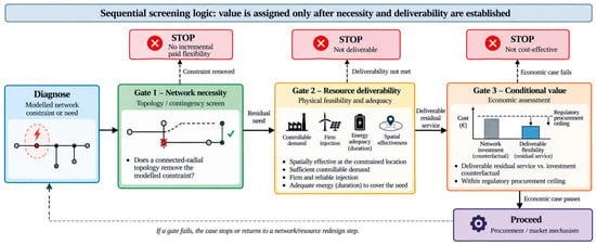
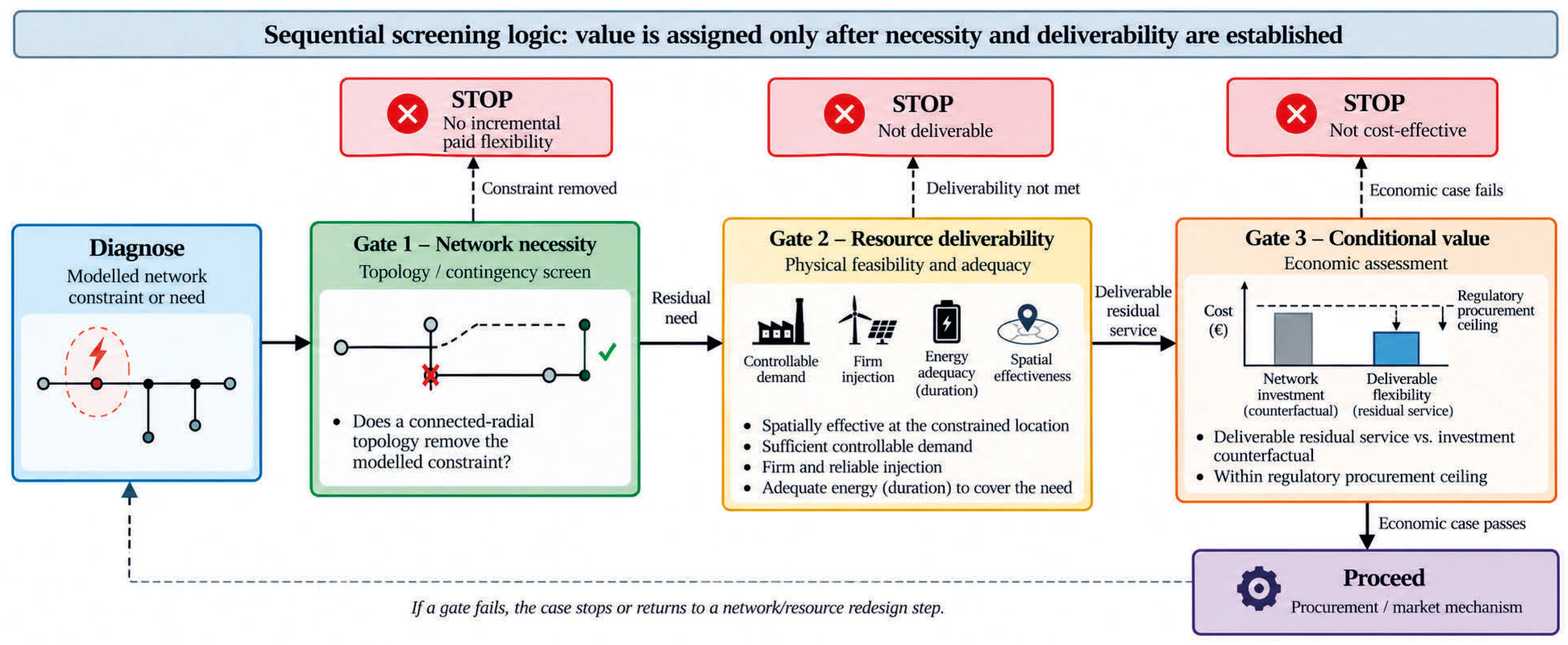
Figure 1 summarises the three-gate logic. A case stops when a network-side action removes the constraint, proceeds to resource screening only when an electrical residual remains, and reaches economic valuation only after that residual is shown to be physically deliverable. Optional value allocation sits outside the core decision path.
Figure 1.
Three-gate framework for screening local flexibility as a non-wires alternative.
2. Materials and Methods
2.1. Research Design: A Sequential Three-Gate Physics-to-Value Framework
The analytical design combines benchmark-based electrical modelling with an empirically grounded temporal and regulatory context. The electrical network is the IEEE 33-bus benchmark, whereas the hourly load shape and flexibility-procurement framework are derived from Lithuanian conditions. This separation avoids presenting benchmark impedances, switching states or nodal loads as observed ESO feeder data. The study is therefore a methodological-regulatory case: the benchmark tests the internal logic of the stopping sequence, while Lithuanian data and rules define the temporal and institutional conditions under which flexibility is interpreted.
Figure 1 summarises the three conditional gates. Gate 1 asks whether a connected-radial electrical topology removes the modelled constraint; if it does, paid flexibility has no incremental value for that state, subject to separate real-world operational permissibility. Gate 2 applies only to a surviving need and tests spatial effectiveness, controllable demand, firm injection and energy adequacy. Gate 3 compares the deliverable residual service with the investment counterfactual and regulatory procurement ceiling. The sequence prevents avoidable network needs, physically infeasible resource assumptions and unsupported economic value from propagating through the appraisal.
2.2. Data, Parameters and Epistemic Status
Table 2 classifies the numerical inputs by epistemic status: observed data, published benchmark parameters, regulatory parameters, scenario assumptions and derived quantities. The 2025 Lithuanian hourly load series from the European Network of Transmission System Operators for Electricity (ENTSO-E) is used only to transfer the observed temporal load shape; absolute national-system MW values are normalised before being applied to the IEEE 33-bus benchmark and are never interpreted as feeder-level demand. The benchmark therefore preserves the electrical structure and spatial load distribution of case33bw while adopting the observed Lithuanian annual time profile. The 4% annual local-growth trajectory is the base planning stress; 3%, 5% and 6% are main sensitivities; and 8%, 10% and 12% are extended zonal stress cases. None is presented as a forecast of Lithuanian national electricity demand or a projection of a specific ESO feeder.
Table 2.
Input data and epistemic status.
Regulatory and financial parameters are analysed separately from observed and benchmark inputs. ESO product requirements provide procurement and resource prequalification context, while the VERT framework provides the regulatory investment counterfactual. Where market values are not observed, cost inputs are explicitly treated as scenario assumptions rather than as Lithuanian flexibility-market bids. Detailed uncertainty, temporal-resolution and resource sensitivities are reported in Supplementary Material S1.
This structure improves transparency and reproducibility and supports the transfer of the framework to distribution systems with different network data, regulatory conditions, or flexibility-resource assumptions.
2.3. Lithuanian Regulatory and Product Counterfactual
Article 401 of the Lithuanian Law on Electricity allows a DSO to procure and use flexibility services in distribution networks, including supply- and demand-side management, demand response, aggregation, energy storage and congestion management, as well as other services required for efficient network operation and development [37]. Under the ESO flexibility-trading framework approved by VERT in 2026, economic assessment and the maximum expenditure for flexibility procurement are determined separately for each network section in which a flexibility need is identified [12]. In the notation used here, the regulatory upper limit is:
Here, is the maximum permitted flexibility expenditure for the relevant network section, x is the number of years for which reconstruction is deferred, C_R is the corresponding network-reconstruction cost, and represents procurement and administrative costs. The denominator of 40 reflects the regulatory depreciation period applied to network reconstruction in the Lithuanian framework [12].
For the gross conceptual comparison, is initially set to zero. Equation (1) therefore reduces to . The resulting value is treated as a regulatory procurement ceiling before administrative costs, not as the economic value of flexibility itself. This distinction is essential because the regulatory ceiling is later compared with the discounted value of the same deferred investment.
In addition to the expenditure cap, the ESO product sets geographical and technical requirements for participating resources. Providers specify the facility location and the flexible or controllable share of capacity. The long-term active-power product requires 100% availability, activation within 15–60 min, and delivery from 60 min to 12 h; contracts may run for no more than three years [11,12].
These provisions motivate a resource-level feasibility assessment. Demand response is bounded by the load that can actually be controlled, while injection-capable resources must satisfy the required active power and, where storage is used, the energy needed over the assumed delivery interval. A battery energy storage system (BESS) that can deliver the required kW is not necessarily able to sustain that power over the full-service duration.
The 8760-point series is used at one-hour resolution to identify planning stress states and construct hourly power and energy adequacy measures. It does not simulate the ESO product’s 15–60 min activation trajectory, intra-hour ramping, 24 h recovery, or provider non-delivery. These provisions are therefore treated as resource-prequalification requirements rather than capabilities demonstrated by the model. Economic valuation is performed only after network necessity and planning-level physical deliverability have been established.
2.4. IEEE 33-Bus Electrical Benchmark, Switch States and Load Zones
The electrical network model is based on the Baran-Wu 33-bus radial distribution benchmark [34] as implemented in MATPOWER case33bw [35]. The benchmark uses a 10 MVA power base and a nominal line-to-line voltage of 12.66 kV. Total nominal demand is 3715 kW and 2300 kVAr. Unless otherwise stated, nodal loads are represented as constant-PQ loads, and bus 1 is the slack bus at 1.0 p.u. The network contains 33 buses and 37 branches. In the normal configuration, L1–L32 are closed and form the connected radial feeder, whereas T33–T37 are normally open tie branches connecting buses 21–8, 9–15, 12–22, 18–33 and 25–29, respectively. Every analysed operating state is required to be connected and radial. Table 3 summarises the benchmark characteristics and base stress quantities used in the analysis.
Table 3.
IEEE 33-bus benchmark characteristics and base stress results.
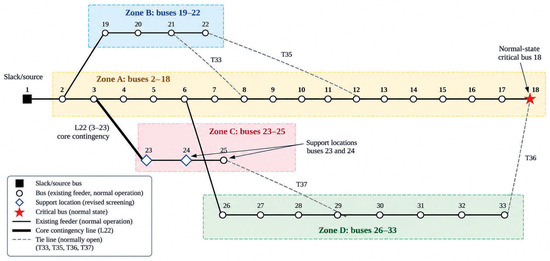
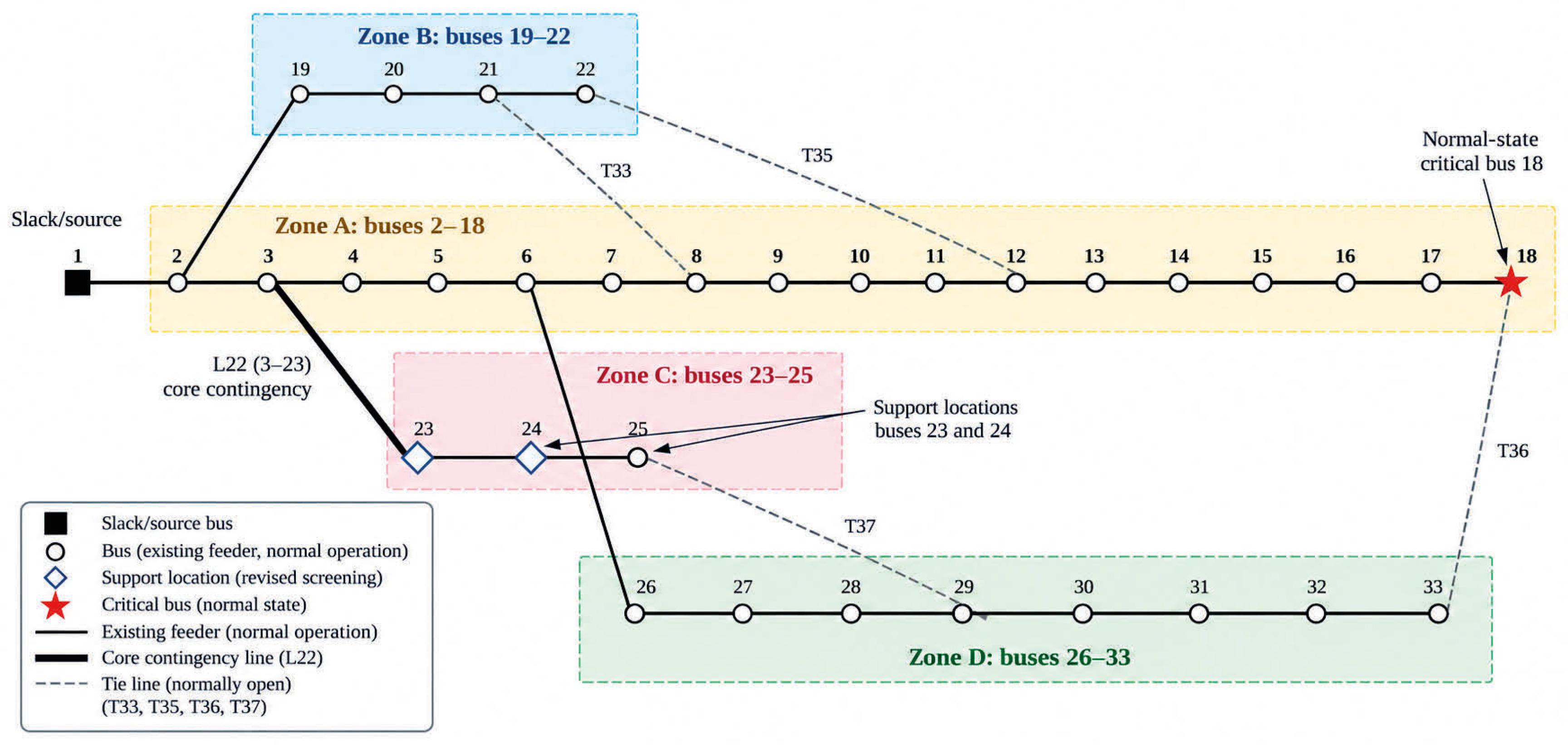
For reporting and comparative analysis, the network is divided into four author-defined load zones. Zone A comprises buses 2–18 (1505 kW, 740 kVAr), Zone B buses 19–22 (360 kW, 160 kVAr), Zone C buses 23–25 (930 kW, 450 kVAr), and Zone D buses 26–33 (920 kW, 950 kVAr). These zones are reporting groups used to compare spatial demand, restoration performance and residual flexibility requirements; they are not attributes of the original IEEE benchmark. Complete busload, branch-impedance and switching-status data are provided in Supplementary Material S1.
Figure 2 presents the benchmark one-line diagram, the four author-defined analytical zones, the normal-state critical bus and the key locations used in the revised STOP/PROCEED cases. In particular, L22 (3–23) is the representative Zone-C gateway contingency, and buses 23–24 are the support locations selected by the expanded Gate-2 analysis.
Figure 2.
IEEE 33-bus benchmark, analytical zones and key locations used in the revised screening cases.
The canonical case33bw dataset does not provide validated continuous or emergency thermal ratings. Consequently, the study does not label any branch as thermally overloaded or infer ampacity congestion. Screening uses connectivity, radiality, power-flow convergence and the analytical bus-voltage criterion. The benchmark tests the decision logic of reconfiguration and location-specific support; quantified material or greenhouse gas savings are not inferred without project-specific reinforcement and life-cycle data.
2.5. Exhaustive Electrical Topology and Zonal Contingency Scenario Design
To avoid selecting a favourable switching state ex ante, the topology layer is exhaustive. Let G = (N,E) denote the 33-bus, 37-branch graph. Every operating topology considered in the normal-state scan is a connected-radial spanning tree. The exact number of spanning trees is obtained from the reduced graph Laplacian, denoted below, by the matrix-tree theorem:
Radiality requires a connected graph with exactly |N| − 1 energised branches:
The contingency space contains every outage of one or two normally closed branches. Therefore,
For each N−1 or N−2 fault state, the 50,751 pre-enumerated spanning trees are filtered so that every failed branch remains open. Each remaining connected-radial candidate is evaluated by the same AC BFS model; the state with the highest minimum bus voltage is reported for the topology-only post-contingency screen. A BFS non-convergence is excluded from voltage compliance counts but is not interpreted as proof that no AC solution exists. The search does not impose switching sequence or count, protection coordination, fault-current limits, communications/SCADA availability, switch availability, restoration time, crew constraints, or operating policy. The candidates are therefore electrically feasible within the benchmark model only, and the best post-fault result is an electrical upper bound on reconfiguration capability rather than a directly dispatchable restoration plan. Table 4 summarises the enumerated normal and contingency scenario space.
Table 4.
Radial-topology and contingency scenario space.
For zonal interpretation, every N−1 fault is assigned to the zone containing the failed normally closed branch. Four gateway cases are then reported in detail: L1 for the Zone-A/source backbone, L18 (2–19) for Zone B, L22 (3–23) for Zone C, and L25 (6–26) for Zone D. L1 is a special systemic case because it disconnects the only slack-source connection to the entire feeder; an exact “Zone A only” outage, with Zones B–D still supplied, is impossible in this single-source benchmark. Gateway cases are evaluated at 3%, 4%, 5% and 6% annual local growth in the main text and at 8%, 10% and 12% in Supplementary Material S1.
2.6. Backward/Forward-Sweep Power Flow and Benchmark Validation
The steady-state operating point of each connected radial topology is calculated with a backward/forward-sweep (BFS) AC power-flow algorithm. The feeder is represented by a balanced single-phase equivalent, loads are constant-PQ, and bus 1 is the slack bus at V1 = 1∠0°. The model therefore represents an aggregated medium-voltage planning case rather than an unbalanced low-voltage feeder.
At bus i, hour t and planning year y, the active net demand and the corresponding per-unit complex power withdrawn from the network are defined as:
Here, and are the benchmark nominal loads, s(t, y) is the common temporal/growth multiplier, and f(i, t, y) is positive active-power flexibility that reduces upstream net demand. Because the FSPs in the screening model provide active-power flexibility only, reactive power is not modified by f.
At BFS iteration k, the current injection at bus i is:
During the backward sweep, branch current is accumulated from downstream buses:
During the forward sweep, bus voltages are updated from the slack bus:
Iterations continue until
Active-power losses are calculated from branch currents and resistances:
With expressed in MVA, Equation (10) yields active losses in MW; the reported values are converted to kW. The solver is validated before any Lithuanian calibration. At the published IEEE-33 nominal load, the normal radial topology yields Vmin = 0.913090 p.u. at bus 18 and active losses of 202.677 kW, closely reproducing the canonical benchmark [34,35].
For scenario screening, the analytical voltage criterion is:
A state is labelled voltage-compliant only when the BFS converges, all load buses remain connected to the slack bus, radiality is maintained and Equation (11) is satisfied. The 0.95 p.u. value is an analytical planning threshold, not a Lithuanian statutory feeder criterion. Sensitivity is therefore evaluated at 0.940, 0.945, 0.950, 0.955 and 0.960 p.u. while holding the physical calibration, hourly profile and year-3 stress state fixed. Because case33bw does not provide validated branch ampacity or MVA ratings, voltage compliance remains narrower than full operational security.
2.7. Lithuanian Hourly Calibration and Local-Growth Scenarios
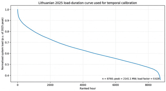
ENTSO-E’s Monthly Hourly Load Values provide a complete 8760 h Lithuanian series for 2025 [33]. The recorded peak is 2141.055 MW, mean load is 1343.934 MW, load factor is 0.628, and annual energy represented by the hourly sum is 11.773 TWh. Only the normalised one-hour temporal shape is transferred to the benchmark feeder:
The benchmark is scaled by s0 so that the normal topology is exactly at Vmin = 0.95 p.u. at the observed 2025 load-shape peak. The resulting s0 = 0.5946806 is a designed boundary condition, not an estimate of an ESO feeder. For planning year y:
The base stress trajectory is g = 4% per year. Growth rates of 3%, 5% and 6% are main-text sensitivities, while 8%, 10% and 12% are extended zonal stress cases in Supplementary Material S1. They represent possible local hot-spot growth associated with connections or electrification and are not forecasts of national Lithuanian demand. Figure 3 shows the resulting normalised 2025 load-duration curve used for hourly temporal calibration.
Figure 3.
Normalised Lithuanian 2025 load-duration curve used for hourly temporal calibration.
2.8. Gate 1: Electrical Incrementality Through Topology Screening
Gate 1 tests whether paid flexibility remains incremental after network-side topology actions. The widely reported IEEE 33-bus minimum-loss reconfiguration, with branches 7, 9, 14, 32 and 37 open [22], is retained as a reference configuration, but Gate 1 is not defined by that single state: the complete connected-radial topology space is screened electrically. A STOP decision is reached when at least one screened candidate satisfies the analytical voltage criterion; whether an equivalent configuration is operationally permissible on a real feeder remains a separate DSO assessment.
Equation (14) is therefore an incrementality rule, not a claim that switching is costless or operationally available. Protection, switching limits, reliability policy and restoration procedures may invalidate an electrically feasible candidate. Threshold sensitivity is interpreted as a decision-boundary test: the framework asks whether the STOP/PROCEED classification persists when the analytical voltage criterion is perturbed while all physical inputs are held fixed.
2.9. Gate 2: Residual-Support Optimisation and Resource Deliverability
If Gate 1 leaves a residual need, the model calculates the minimum positive active-power support required to restore the voltage criterion. Spatial robustness is tested rather than imposed through four arbitrary buses. For the normal fixed-topology comparator, all 32 load buses are screened individually, all 496 two-bus combinations are evaluated, and a 41-start all-bus Sequential Least Squares Programming (SLSQP) optimisation cross-checks the best result. For the L22 PROCEED case, the highest Vmin post-fault topology is first evaluated with all load buses eligible; a topology-sensitive Gate-2 search then identifies a lower-support connected-radial candidate, which is cross-checked with all-bus and Zone-C-only siting. Multi-start convergence demonstrates the numerical stability of the reported candidate but is not presented as a formal global-optimality proof for the nonlinear AC problem.
Net flexibility is not equated with demand curtailment. For FSP i and hour t:
Demand reduction is bounded by contemporaneous controllable load:
The parameter is a scenario bound, not an empirical estimate. Values of 0%, 20%, 50% and 100% expose how the technology mix changes as controllable demand expands. Any residual f − d must be supplied by an injection-capable resource such as BESS discharge or sufficiently firm controllable generation. In this study, ‘resource-feasible’ therefore means planning-level feasibility under the stated demand, injection, efficiency, SOC and duration assumptions; it does not establish actual provider deliverability. Actual service delivery requires provider-specific verification of controllable load, firm power and energy capability, activation, recovery, availability and other applicable product requirements. Firm injection is not synonymous with storage, and device-specific converter, control and power-quality compliance remain outside the steady-state active-power model [25,26]. For a BESS,
For the fixed-topology chronological comparator, binding residual-injection hours are grouped into contiguous one-hour model intervals. For event e,
A lower bound on battery nameplate energy is then:
Here, is the usable fraction of the nominal state-of-charge (SOC) range. Equation (21) is a lower-bound planning adequacy measure; project design also requires a reserve margin, inverter sizing, auxiliary consumption, degradation, recharge capability and site-specific reliability criteria. For the deterministic L22 contingency, no outage-duration distribution is available, so the 1/2/4/8/12 h storage results are treated as product-duration sensitivities rather than predicted outage durations. The hourly model does not validate 15–60 min activation or 24 h recovery.
2.10. Gate 3: Conditional Economic Valuation
Economic valuation is performed only if the preceding screens leave a genuine, physically deliverable residual need. Equation (1) gives the Lithuanian regulatory ceiling. A second benchmark asks how much deterministic present value is created solely by postponing the same fully deferrable capital expenditure. If the reinforcement cost is deferred x years at a discount rate r:
ESO’s published 2026 weighted average cost of capital (WACC) of 5.77% is used as r [36]. The calculation is normalised to EUR 1 million of reinforcement capital expenditure (CAPEX) and is repeated over genuinely deferrable CAPEX shares, rather than assuming that every real project is fully postponable. The comparison excludes construction-cost uncertainty, operating-cost differences and real-option value.
For a residual flexibility requirement, procurement cost over the horizon is:
The break-even reservation price for a chosen value benchmark V is:
No public Lithuanian market-clearing bids are assumed. EUR 100/kW-year reservation and EUR 100/MWh activation are explicit scenario prices, not estimates of ESO market prices. For the L22 β = 20% illustration, the year-3 planning-level resource-feasible capacity is conservatively held constant across the three-year reservation horizon. Because no empirical outage frequency or repair-time distribution is imposed, activation cost is reported only per assumed event duration rather than as an expected annual cost.
2.11. Optional Post-Valuation Cooperative Allocation Illustration
For transparency, Supplementary Material S1 retains a three-player transferable-utility illustration based on the legacy fixed-topology buses 18 and 33. Only coalitions containing the DSO can create network-deferral value. For coalition S,
The Shapley allocation benchmark for player i uses i to denote the player set excluding i, and S + i to denote coalition S with player i added:
This calculation is an optional post-valuation marginal-contribution benchmark only. It is not a fourth gate, a research question, a representation of a heterogeneous provider market or a substitute for competitive procurement. The numerical results are retained in Supplementary Material S1 rather than in the core Results section.
2.12. Reproducibility and Software Disclosure
All calculations were implemented in Python 3.13.5 using NumPy 2.3.5 and SciPy 1.17.0, with Numba 0.65.1 used to accelerate exhaustive spanning-tree and contingency enumeration. Supplementary Material S1 contains the input/source register, IEEE 33-bus bus and branch data, the 8760 h Lithuanian load profile, and complete normal, N − 1, and N − 2 electrical screening. It also contains voltage-threshold sensitivity; expanded single-bus, pair, and all-bus siting checks; L22 Gate-2 and resource calculations; duration, efficiency, and SOC sensitivities; conditional L22 economics; temporal-resolution and uncertainty frameworks; and the optional cooperative-allocation illustration. The spanning-tree count was independently verified by the matrix-tree theorem and exhaustive enumeration, and principal numerical checkpoints were rerun from source inputs before finalisation. Calculation code is available from the corresponding author on reasonable request.
3. Results
3.1. Benchmark Validation and Scope Marker
At the unscaled published IEEE 33-bus load, the BFS model yields 202.677 kW active losses and Vmin = 0.913090 p.u. at bus 18, closely reproducing the canonical benchmark [34,35]. After calibration, the normal topology is exactly at the 0.95 p.u. analytical threshold at the 2025 Lithuanian load-shape peak. This is a designed boundary condition. All absolute voltages, losses, support quantities and contingency outcomes reported below are benchmark-specific and should not be extrapolated to an ESO feeder; the transferable result is the screening logic. Table 5 reports the principal electrical validation and topology-screen checkpoints.
Table 5.
Electrical validation and topology-screen checkpoints.
3.2. Electrical Topology and Contingency Screening
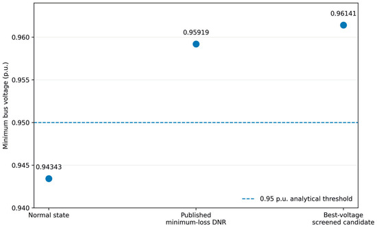
The exact enumeration confirms 50,751 connected-radial configurations. At the year-3 4% stress point, 50,313 converge and 4403 satisfy the base 0.95 p.u. criterion. The maximum-Vmin state reaches 0.961412 p.u.; the published minimum-loss DNR reaches 0.959190 p.u. Threshold sensitivity shows that the central STOP/PROCEED architecture is stable from 0.945 to 0.955 p.u.: the normal state fails, while the topology screen contains a compliant normal-state candidate and the L22 contingency remains below criterion. At 0.940 p.u. the normal state and L22 both pass, whereas at 0.960 p.u. the published minimum-loss DNR fails, but the best-voltage radial candidate still passes. The magnitude and even existence of a residual need are therefore threshold-dependent near decision boundaries, which is why 0.95 p.u. is treated as an analytical assumption rather than a Lithuanian limit.
Post-contingency results distinguish topological restorability from voltage adequacy. Of 32 N − 1 outages, 31 have at least one connected-radial post-fault candidate and 26 are voltage-compliant at the year-3 4% stress point. L1 is the only topologically non-restorable event because it is the sole source-side connection. Zone B is compliant in all four N − 1 cases, Zone C contains two restorable but non-compliant gateway cases (L22/L23), and Zone D contains the weak downstream L29/L30 corridor. These patterns imply different engineering mechanisms rather than a single generic ‘weakest zone’. Table 6 summarises the corresponding zone-level N − 1 vulnerability pattern.
Table 6.
Zone-level N − 1 vulnerability at the year-3 4% stress point.
The N − 2 stress set contains 496 double-branch pairs: 419 are topologically restorable, and 253 are voltage-compliant after electrical reconfiguration. All three within-Zone-C double contingencies are topologically non-restorable, and only 2 of 24 C–D pairs are voltage-compliant. These are deterministic vulnerability screens, not failure-probability-weighted reliability indices or a claim of a statutory Lithuanian N − 2 requirement.
The four representative gateway cases make the mechanism explicit. L1 is a source-redundancy problem: no internal tie can reconnect the slack source. L18 in Zone B is restored above 0.95 p.u. at the base stress. L22 in Zone C is topologically restorable, but no topology-only candidate reaches 0.95 p.u.; it therefore becomes the main positive residual case. L25 at the Zone-D gateway is robust through the main growth range, whereas the internal L29/L30 corridor is sensitive. The reported open sets are electrical candidates and include the failed branch itself. Table 7 reports the representative gateway cases used for the zonal interpretation.
Table 7.
Representative zonal gateway contingencies after topology-only screening.
The practical implication is not a monetary zone ranking. Zone A calls for source-path redundancy or an explicitly modelled islanding solution. Zone B requires no paid local support in the base stress if equivalent switching is available. Zone C is the clearest local support or reinforcement case, while Zone D points to downstream sectionalisation or local reinforcement. Project-specific ratings, switching permissions, and CAPEX would be required to rank these interventions financially.
3.3. Gate 1 STOP Case: Normal Year-3 State
At the year-3 4% peak, the normal topology falls to 0.943429 p.u. at bus 18. The published minimum-loss DNR raises Vmin to 0.959190 p.u., while the best-voltage screened radial candidate reaches 0.961412 p.u. Because the complete electrical topology screen contains compliant candidates, the incremental paid-flexibility requirement is zero in this benchmark state if an equivalent configuration is operationally permissible. The result is therefore a STOP decision, not a general claim that flexibility has no value. Figure 4 compares the normal state with the published DNR and the best-voltage screened radial candidate.
Figure 4.
Electrical topology-screen result for the normal year-3 stress state.
The STOP decision is also robust over the central threshold sensitivity: it persists at 0.945, 0.950 and 0.955 p.u. At 0.960 p.u., the published minimum-loss DNR no longer passes, but another screened radial candidate does. This reinforces the methodological point that Gate 1 is the topology-space screen rather than a test of one preselected DNR state.
3.4. Positive Residual Case: Zone C/L22
L22 (3–23) disconnects buses 23–25 before restoration, representing 930 kW of nominal benchmark demand. The topology-only screen evaluates 5889 connected-radial post-fault candidates, of which 5824 converge, but none satisfy 0.95 p.u. The highest no-flex Vmin is 0.942934 p.u. with the open set {L6, L9, L14, L22, L31}. Gate 2 therefore cannot be bypassed. Importantly, the highest-Vmin topology is not the minimum-support topology: expanded siting and topology-sensitive screening identify the open set {L7, L9, L14, L22, L31}, which requires 222.106 kW at buses 23 and 24. Restricting eligibility to Zone C buses 23–25 gives the same minimum, so no locality penalty is observed in this benchmark case. Table 8 summarises the topology and siting robustness of the resulting L22 residual-support requirement.
Table 8.
Zone-C L22 residual-support robustness.
The 18.9% reduction from the former 273.8 kW value shows why both topology and siting must be audited before a residual service is priced. The revised 222.106 kW quantity is the benchmark electrical requirement for the selected L22 Gate-2 candidate; it is not a Lithuanian procurement quantity or a formal proof of the mixed-discrete global optimum.
3.5. Gate 2: Resource Deliverability for L22
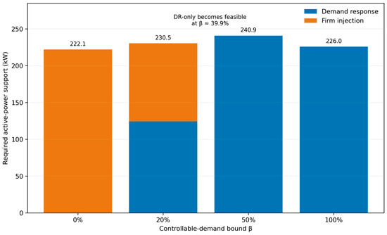
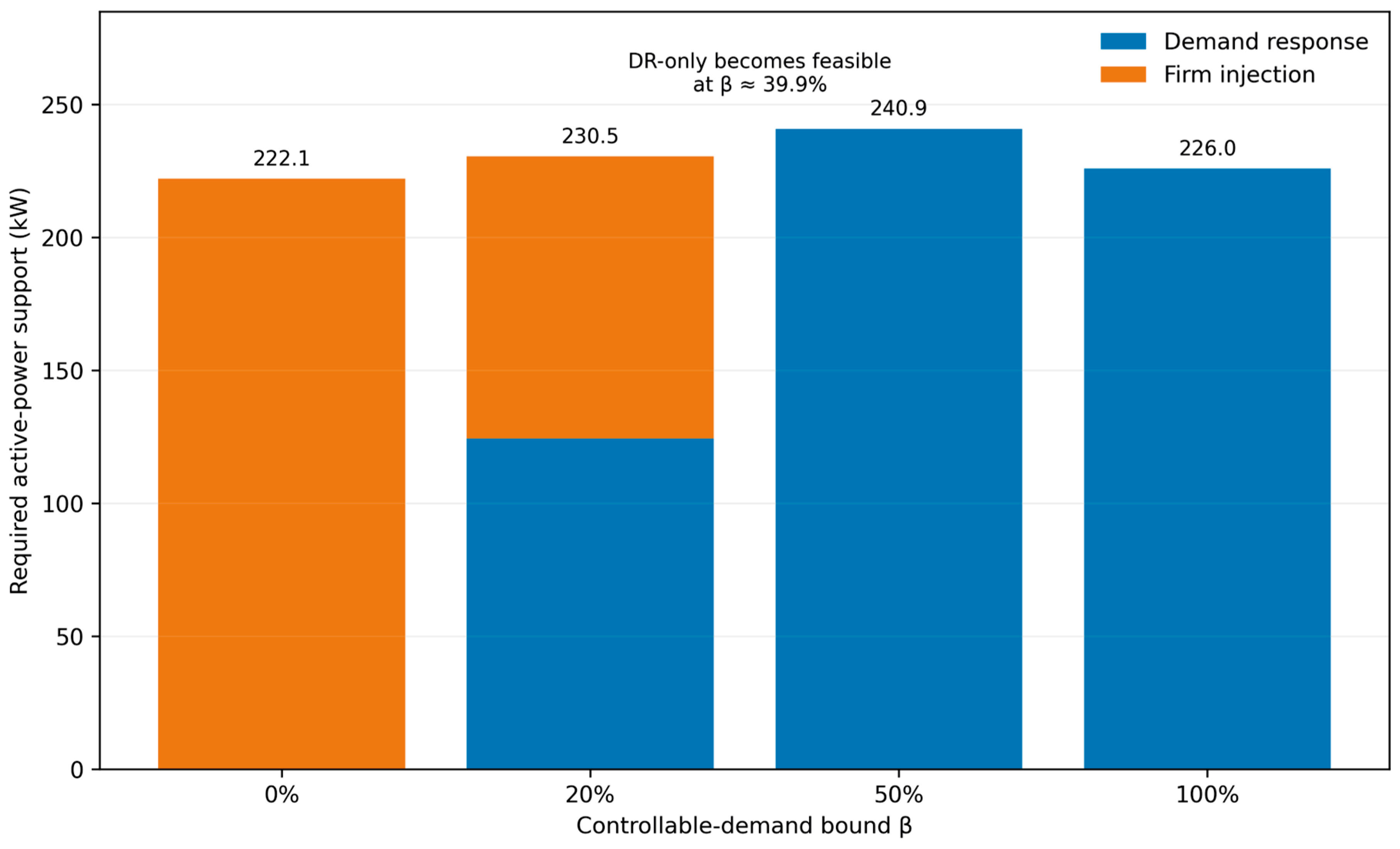
The 222.106 kW electrical requirement does not uniquely determine a technology. With no controllable demand, all support must be firm injection. Under the base bound, 124.422 kW can be supplied by demand response, but 106.061 kW of firm injection remains necessary. The resulting planning-level constrained portfolio totals 230.483 kW because per-bus demand limits restrict the spatial allocation of demand response and therefore force a less electrically effective support mix. A DR-only solution becomes feasible at approximately β = 39.9%. Thus, the same network need can map to injection-only, hybrid, or DR-only service depending on the resource envelope. These portfolios are planning-level feasibility envelopes under assumed resource parameters, not verified provider capabilities.
For storage-backed firm injection, the required energy is duration-dependent. Under β = 20%, 95% discharge efficiency and 80% usable SOC, the lower-bound nameplate rises from about 0.140 MWh for a 1 h service to 1.675 MWh for 12 h. Across plausible efficiency/SOC assumptions, the 12 h lower bound ranges from approximately 1.46 to 2.02 MWh. These are product-duration sensitivities, not predicted L22 outage durations, and they do not validate sub-hour activation, recharge or repeated-event capability. Table 9 reports the resource-envelope and duration-conditioned storage bounds, while Figure 5 visualises the resource-composition shift across controllable-demand scenarios.
Table 9.
L22 resource envelope and duration-conditioned storage lower bounds.
Figure 5.
Resource composition required for the Zone-C L22 residual-support case under alternative controllable-demand bounds.
The planning implication is to tender the required network service rather than infer a technology from the headline kW. Provider prequalification must then demonstrate controllable load, firm-injection capability, energy duration, availability and the applicable response/recovery requirements. A BESS is one possible firm-delivery technology, not a predetermined NWA solution.
3.6. Gate 3: Conditional Economic Value for L22
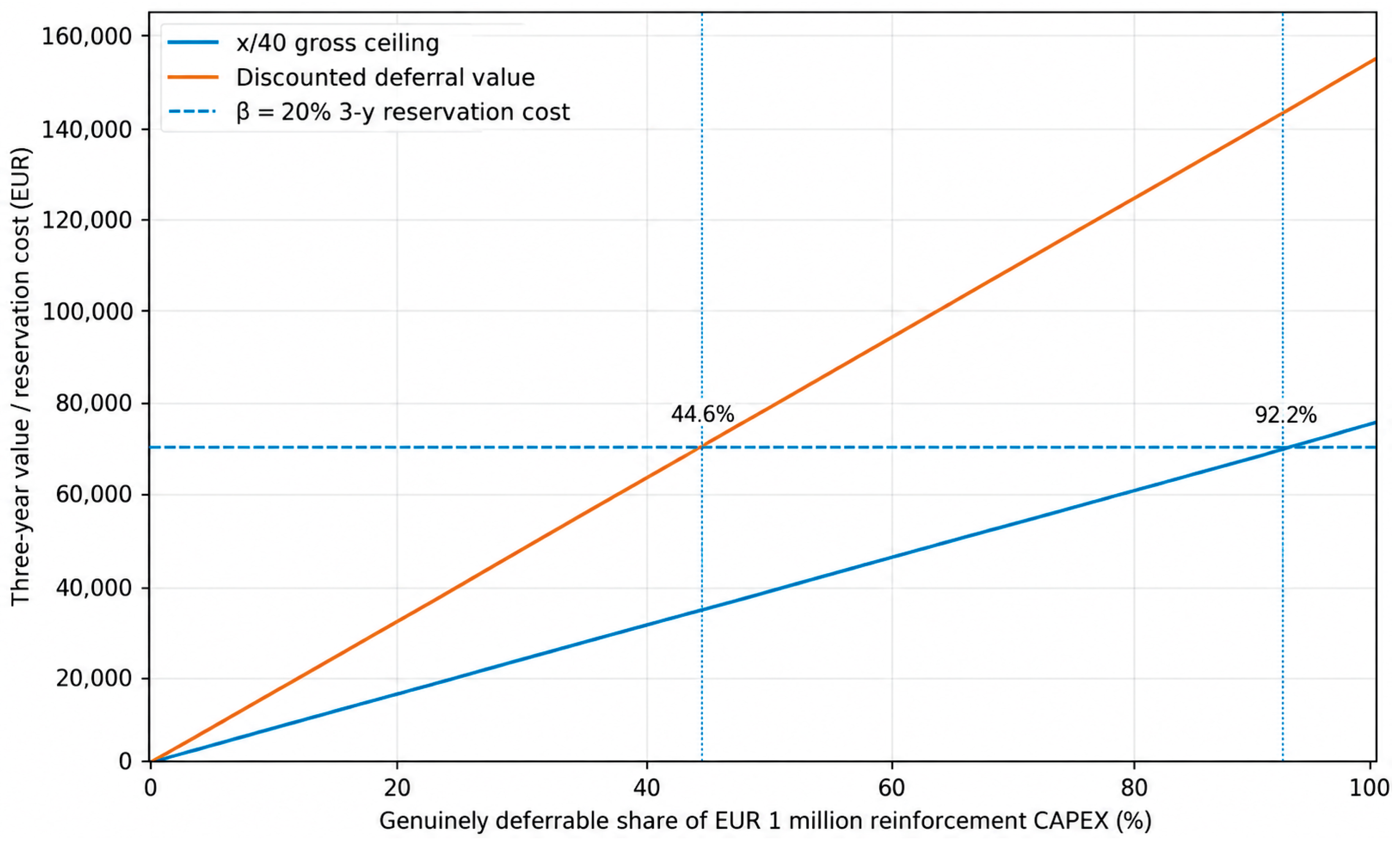
Gate 3 links the positive residual case to a conditional investment counterfactual. For β = 20%, the planning-level resource-feasible L22 portfolio requires 230.483 kW of contracted support. For a conservative reservation-cost screen, that year-3 capacity is held constant for three years, giving 691.450 kW-year. At the illustrative EUR 100/kW-year reservation price, the reservation cost is EUR 69,145 before activation and administration.
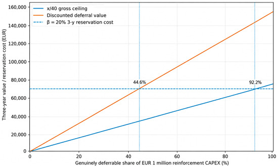
Per EUR 1 million of genuinely deferrable reinforcement CAPEX, the three-year x/40 gross ceiling is EUR 75,000 and the deterministic discounted deferral value at 5.77% WACC is EUR 154,891. The reservation-only L22 screen therefore passes both full-deferral benchmarks, but the regulatory headroom is narrow. At the illustrative price, the minimum genuinely deferrable CAPEX share is approximately 92.2% under x/40 and 44.6% under the discounted-deferral benchmark. Economic eligibility is therefore highly conditional on project scope rather than implied by technical feasibility alone. Figure 6 shows the sensitivity to the genuinely deferrable CAPEX share, and Table 10 reports the corresponding Gate-3 decision metrics.
Figure 6.
Conditional L22 economic screen as a function of the genuinely deferrable share of reinforcement CAPEX.
Table 10.
Conditional L22 Gate-3 decision metrics.
The two value measures answer different questions. Equation (1) is a regulatory procurement ceiling linked to the regulated reconstruction period, whereas Equation (22) measures the deterministic time value of postponing an otherwise identical capital payment. Neither is an observed market price, and the 40-year regulatory denominator should not be interpreted as the remaining physical life of a particular feeder asset.
Activation cost is kept separate because the deterministic L22 contingency has no empirical event frequency. At EUR 100/MWh, full-power activation would cost only about EUR 23 for 1 h and EUR 277 for 12 h per event, but multiplying those figures into an annual expectation would require failure frequency and restoration-duration data that the benchmark does not contain.
3.7. Fixed-Topology and Hourly Comparator
The original fixed-normal-topology case is retained only to illustrate locational effectiveness and chronological energy persistence. Removing the former four-bus siting restriction confirms that buses 18 + 33 form the best of all 496 two-bus combinations at 143.919 kW. A 41-start all-bus optimisation converges to the same active locations and an essentially identical objective. The best single-bus solution is bus 15 at approximately 286.519 kW. These values are not procurement requirements when Gate 1 can remove the normal-state constraint.
The same comparator provides the only 8760 h event chronology in the study. Under 4% local growth, voltage violations occur for 21 h in year 1, 82 h in year 2 and 230 h in year 3, with 8.941 MWh of total three-year net activation. At β = 20%, the longest residual-injection event spans 11 consecutive one-hour model intervals and requires 659.66 kWh delivered, corresponding to a central lower-bound BESS nameplate of about 0.868 MWh. This is an hourly resolution planning adequacy result, not validation of 15-60 min activation or 24 h recovery.
3.8. Integrated Decision Rule
Table 11 condenses the practical stopping logic. The same benchmark can produce a STOP case, a positive residual PROCEED case, or a structural network problem for which local flexibility is not the primary intervention. The framework therefore returns an intervention direction and a statement of missing real-feeder evidence rather than forcing every scenario into a flexibility valuation.
Table 11.
Integrated benchmark decision matrix.
4. Discussion
4.1. The Main Methodological Finding: Flexibility Value Must Be Earned Sequentially
The central finding is not that flexibility is always preferable to reinforcement, nor that a particular storage capacity should be installed on an IEEE feeder. It is that NWA value emerges only after an ordered sequence of prerequisite tests. This resolves three category errors: a need calculated before network-side screening is not necessarily incremental; a net active-power variable is not automatically demand response; and a regulatory spending limit or discounted system value is not automatically a market price.
The normal-state STOP result illustrates the first point. A fixed topology appears to require 143.919 kW, but the complete electrical topology screen contains a radial candidate above the analytical threshold. The correct incremental paid-flexibility quantity is therefore zero in that benchmark state if an equivalent configuration is operationally permissible. This is consistent with Valarezo et al. [20,21], who show that DNR can materially change flexibility needs and provider eligibility. The procedural contribution here is to make that network-side screen an explicit stopping rule before procurement value is assigned.
4.2. Engineering Meaning of STOP, PROCEED and Zonal Vulnerability
The contingency results show why a single ‘weakest zone’ label is inadequate. Zone A is structurally critical because L1 is the sole source connection; local support cannot restore a disconnected source path under the non-islanding model. Zone B is comparatively robust because its 360 kW lateral can be resupplied through alternative electrical paths without violating the base criterion. Zone C is different: loss of the 3–23 gateway forces the 930 kW lateral onto a weaker alternative path, and topology alone remains insufficient. Zone D’s gateway is comparatively robust, whereas its long downstream corridor contains the internal L29/L30 weakness. Bus 30 also carries a large reactive component (200 kW and 600 kVAr), which increases voltage sensitivity.
The L22 case provides the positive residual counterexample needed to interpret the framework practically. The highest no-flex Vmin topology is not the lowest-support topology, and replacing the legacy four-bus siting restriction lowers the residual from 273.8 to 222.106 kW. The all-bus optimum lies entirely in Zone C at buses 23 and 24, so the benchmark does not impose an artificial locality penalty. This is precisely the point at which the framework changes from ‘screen the network’ to ‘specify a local service’.
The fixed-topology 143.919 kW result remains useful only as a locational comparator. The all-bus audit shows that two electrically complementary locations can require roughly half the support of the best single location, demonstrating that flexibility quantity is a network-location property rather than a fungible system-wide capacity number.
The practical implication is intervention-specific. A planner should not respond to Zone A, Zone C and Zone D with the same product: source redundancy, local support/reinforcement and downstream sectionalisation are different engineering problems. The sequential framework is therefore intended to classify what problem remains before choosing a market or infrastructure solution.
This interpretation also bounds the claims of the exhaustive search. Connected-radial candidates are electrically feasible under the model, but protection coordination, switching sequence/count, communications, equipment status and restoration procedures may shrink the real operational set substantially. The topology results should therefore be read as an electrical upper bound on what reconfiguration could remove, not as an immediately executable DSO restoration plan.
4.3. Resource Deliverability and Temporal Resolution
Gate 2 shows that a network-support requirement is not itself a technology specification. In L22, β = 20% produces a hybrid portfolio of 124.422 kW demand response and 106.061 kW firm injection, whereas DR-only becomes feasible at about β = 39.9%. The total contracted kW is not monotonic in β because per-bus controllable-load bounds force different spatial allocations. Firm injection may be supplied by storage or sufficiently firm controllable generation; converter, control, power-quality and other asset-specific requirements remain separate from the steady-state active-power screen [25,26].
Storage illustrates the temporal dimension. At β = 20%, the central lower-bound nameplate requirement increases from roughly 0.14 MWh at 1 h to 1.67 MWh at 12 h, and varies further with discharge efficiency and usable SOC. These figures test duration-conditioned energy adequacy, not a predicted L22 outage duration or a complete battery design. Recharge, degradation, reserve margin and repeated-event reliability remain outside the screen.
The one-hour temporal model also cannot establish compliance with ESO’s 15–60 min activation or 24 h recovery provisions. Its valid role is planning-level identification of hourly stress, multi-hour persistence and energy adequacy. A procurable service would still require provider-specific evidence on sub-hour response, ramping, recovery and availability.
4.4. Conditional Economic Value, Uncertainty and Optional Allocation
The L22 economic screen makes the investment counterfactual explicit. At the illustrative EUR 100/kW-year reservation price, the β = 20% portfolio costs about EUR 69,145 over three years before activation and administration. That fits below the EUR 75,000 gross x/40 ceiling only when roughly 92% or more of the normalised EUR 1 million project is genuinely deferrable; the deterministic NPV screen crosses at about 45%. A technically feasible service is therefore not automatically an economic NWA: project scope, asset condition, remaining life and the timing of the reinforcement trigger determine how much CAPEX can actually be postponed.
The x/40 ceiling and discounted deferral value should remain conceptually separate. The first is a regulatory procurement limit; the second is the deterministic time value of paying the same capital cost later. Real-options work shows that postponement can carry additional value when future demand and investment conditions are uncertain [38], but that option value is outside the present deterministic calculation. The analysis does not model probability-weighted load growth, renewable output, provider availability, bids, outage frequency, or reinforcement timing. Instead, uncertainty is addressed through deterministic decision-boundary sensitivities in growth, voltage criterion, controllable demand, duration, efficiency/SOC, and deferrable CAPEX. A real feeder could retain the same gate order while replacing these envelopes with stochastic, robust, or chance-constrained inputs. Optional Shapley allocation is retained only in S1 as a limited marginal-contribution illustration [28,29,30,31,32]; actual remuneration would be determined by bids and the applicable procurement mechanism, whose European designs remain heterogeneous [39,40].
4.5. Sustainability Implications
The sustainability contribution of the framework is primarily resource and investment efficiency rather than a claimed carbon saving. Screening electrical topology before buying flexibility reduces the risk of paying for a non-incremental service; screening resource deliverability avoids treating physically impossible demand reduction as a credible alternative to reinforcement; and separating regulatory expenditure limits from deferral value improves transparency in infrastructure-versus-market decisions. These mechanisms can support better use of existing grid assets, defer premature construction and enable distributed-resource integration [1,2,5,20].
No CO2 reduction is calculated. Demand shifting or storage operation does not automatically reduce emissions; the effect depends on marginal generation, losses, charging time and embodied impacts. Avoided reinforcement likewise has material implications that cannot be quantified without project-specific life-cycle inventory. The sustainability claim is therefore bounded to system adaptability, infrastructure resource efficiency, transparent economic governance and the integration of distributed flexibility, consistent with current work on operationalising demand flexibility [27].
4.6. External Validity, Uncertainty and Limitations
First, the electrical network is the IEEE 33-bus benchmark, not an ESO feeder. Lithuanian data provide the temporal load shape and institutional context only. Absolute kW, voltage, loss and contingency values therefore should not be transferred directly to Lithuanian planning. The appropriate external use is procedural: a real case would replace topology, impedances, ratings, loads, DER profiles and switching permissions while retaining the stopping sequence.
Second, 0.95 p.u. is an analytical planning threshold rather than a validated Lithuanian feeder criterion. The dedicated 0.940–0.960 sensitivity demonstrates where decision classifications change, but it does not substitute for the applicable DSO voltage and power-quality rules. The case33bw data also lack validated thermal ratings, so the study diagnoses voltage adequacy and path sensitivity rather than ampacity congestion.
Third, the exhaustive connected-radial search represents electrical rather than operational feasibility. Protection coordination, fault-current limits, switching sequence and frequency, remote-control capability, equipment availability, crew procedures, restoration time and reliability policy are not modelled. N − 1/N − 2 results are deterministic vulnerability screens without failure probabilities, repair times or interruption-cost metrics; N − 2 is a stress test, not a Lithuanian statutory security criterion. BFS non-convergence is treated only as numerical exclusion, not proof that no AC solution exists.
Fourth, resource inputs are scenario envelopes rather than provider measurements. β is not derived from customer baselines; active-power flexibility is modelled without reactive-power optimisation; BESS calculations are lower-bound adequacy checks without recharge, degradation or revenue stacking; and the hourly model does not validate sub-hour activation or 24 h recovery. Renewable generation variability and provider non-delivery are not assigned probabilities.
Fifth, the economic comparison is normalised and deterministic. Only the genuinely deferrable portion of a real project is relevant, and the 40-year regulatory denominator is not the same as physical asset life. Construction-cost escalation, maintenance differences, taxes, residual value, market-price uncertainty, option value and stochastic reinforcement timing are excluded. No observed Lithuanian FSP bids or contingency frequencies are used. These limitations prevent the benchmark from being interpreted as a project recommendation while preserving its role as a transparent decision-boundary study.
4.7. Implications for a Real Lithuanian Feeder Study
Applying the framework to an anonymised ESO feeder would require the normal topology and permissible alternatives, branch impedances and ratings, transformer limits, nodal or customer-group load and DER profiles, protection and switching rules, provider response and availability data, and the planned reinforcement scope and cost. Gate 1 would use the actual operational topology set. Gate 2 would use measured or contracted resource envelopes, sub-hour response, and storage-dispatch limits. Gate 3 would use the genuinely deferrable project scope, expected event use, and observed or elicited market prices. Optional allocation analysis, if desired, would then use the actual provider set and procurement mechanism rather than the three-player illustration.
The same logic maps naturally to intervention planning. NWA-0 denotes no additional action; NWA-R denotes network reconfiguration; NWA-F denotes flexibility only; and NWA-RF denotes reconfiguration plus flexibility. Conventional alternatives include local conductor or feeder reinforcement, voltage-control equipment, transformer uprating and new supply paths. In the benchmark, the normal year-3 state maps to NWA-R, Zone C/L22 to NWA-RF or reinforcement depending on Gate 2–3 results, Zone A to source-redundancy investment, and the downstream Zone-D corridor to sectionalisation/local reinforcement analysis. This is an intervention taxonomy, not an optimised investment plan.
5. Conclusions
This study shows that local flexibility should not be assigned NWA value at the start of a planning analysis. The relevant sequence is to establish whether the network need remains after network-side actions, determine whether the residual service is planning-level resource-feasible under explicit demand, injection and energy assumptions, and only then test whether procurement can credibly defer network expenditure. Passing Gate 2 in this study does not establish actual service deliverability: a procurable service still requires verified provider-specific capability, including controllable load, firm power and energy, activation, recovery and availability. The methodological contribution is this ordered and explicitly terminating decision logic: a case may stop after reconfiguration, proceed to a resource screen, or fail at the economic stage without forcing every scenario through the same valuation chain.
The benchmark application illustrates why this distinction matters. The normal year-3 stress state is a STOP case because the screened connected-radial topology space contains an electrically compliant alternative, whereas the Zone-C L22 contingency is a PROCEED case because topology alone is insufficient and a local residual support requirement remains. The latter is concentrated at buses 23–24 and, depending on the controllable-demand envelope, can be supplied by demand response, firm injection, or a hybrid portfolio. Other zones reveal different engineering mechanisms: Zone A is primarily a source-redundancy problem, Zone B is comparatively robust after reconfiguration, and Zone D contains a downstream internal weakness. These differences show why a single generic flexibility quantity or ‘weakest zone’ ranking is not an adequate planning output.
The economic interpretation is equally conditional. A technically feasible flexibility service has investment value only if it can postpone a genuinely deferrable part of a real network project, and the regulatory expenditure ceiling, discounted deferral value and market remuneration should not be treated as interchangeable quantities. The reported electrical results are benchmark-specific, the 0.95 p.u. threshold is an analytical planning assumption rather than a Lithuanian statutory limit, and the topology screen represents an electrical upper bound rather than a directly executable DSO restoration plan. A real Lithuanian feeder application would therefore require feeder-specific ratings, switching and protection rules, load and DER forecasts, provider availability and response data, and project-specific reinforcement scope and cost. Those inputs would change the numerical results, but not the three-gate logic used to decide whether flexibility should be valued at all.
Supplementary Materials
The following supporting information can be downloaded at https://www.mdpi.com/article/10.3390/su182110726/s1: Supplementary Material S1 (Supplementary_Material_S1.xlsx). The workbook contains the input/source register; IEEE 33-bus bus and branch data; the complete 8760 h Lithuanian load profile; exhaustive normal, N − 1, and N − 2 electrical screening; voltage-threshold and growth sensitivities; expanded flexibility-location audits; L22 residual-support, resource, and conditional economic calculations; BESS duration, efficiency, and SOC checks; temporal-resolution and uncertainty frameworks; fixed-topology chronological comparators; and the optional cooperative-allocation illustration.
Author Contributions
Conceptualization, G.Š. and I.M.; methodology, G.Š. and I.M.; software, G.Š. and I.M.; validation, G.Š.; formal analysis, G.Š. and I.M.; investigation, G.Š. and I.M.; data curation, I.M.; writing—original draft, G.Š. and I.M.; writing—review and editing, G.Š. and I.M.; visualization, I.M.; supervision, G.Š. All authors have read and agreed to the published version of the manuscript.
Funding
This research received no external funding.
Institutional Review Board Statement
Not applicable. The study did not involve humans, animals or identifiable personal data.
Informed Consent Statement
Not applicable.
Data Availability Statement
All data supporting the reported numerical analysis are included in Supplementary Material S1 (Supplementary_Material_S1.xlsx). The Lithuanian hourly load series is derived from ENTSO-E Power Statistics, and the benchmark electrical network is based on MATPOWER case33bw. The workbook contains source inputs, scenario assumptions, exhaustive topology and contingency outputs, threshold and siting sensitivities, L22 Gate-2 and Gate-3 calculations, and reproducibility checkpoints used in the manuscript. Calculation code is available from the corresponding author on reasonable request.
Acknowledgments
The authors reviewed and verified all sources, calculations, numerical results and interpretations, edited all outputs, and take full responsibility for the content of this publication.
Conflicts of Interest
The authors declare no conflict of interest.
Abbreviations
| ACER | Agency for the Cooperation of Energy Regulators |
| BESS | battery energy storage system |
| CAPEX | capital expenditure |
| DER | distributed energy resource |
| DNR | distribution network reconfiguration |
| DR | demand response |
| DSO | distribution system operator |
| ENTSO-E | European Network of Transmission System Operators for Electricity |
| FSP | flexibility service provider |
| NPV | net present value |
| NWA | non-wires alternative |
| SOC | state of charge |
| VERT | Lithuanian National Energy Regulatory Council |
| WACC | weighted average cost of capital |
References
- International Energy Agency (IEA). The Value of Demand Flexibility: Benefits Beyond Balancing; IEA: Paris, France, 2025; Available online: https://www.iea.org/reports/the-value-of-demand-flexibility (accessed on 29 August 2026).
- Strbac, G.; Pudjianto, D.; Aunedi, M.; Djapic, P.; Teng, F.; Zhang, X.; Ameli, H.; Moreira, R.; Brandon, N. Role and value of flexibility in facilitating cost-effective energy system decarbonisation. Prog. Energy 2020, 2, 042001. [Google Scholar] [CrossRef] [Scilit]
- European Parliament and Council. Directive (EU) 2019/944 of 5 June 2019 on Common Rules for the Internal Market for Electricity and Amending Directive 2012/27/EU. Off. J. Eur. Union 2019, L158, 125–199. [Google Scholar]
- Agency for the Cooperation of Energy Regulators (ACER). Decision No. 05-2025 on the Type and Format of Data and the Methodology for TSOs’ and DSOs’ Flexibility Needs Analysis, 28 July 2025; ACER: Ljubljana, Slovenia, 2025; Available online: https://www.acer.europa.eu/acer-decision-no-05-2025-type-and-format-data-and-methodology-tsos-and-dsos-flexibility-needs-analysis (accessed on 7 October 2026).
- Messias, R.; Carvalho, P.M.S.; Sousa, J. Hybrid distribution network planning to incorporate virtual capacity from distributed flexibility resources. Util. Policy 2025, 93, 101892. [Google Scholar] [CrossRef] [Scilit]
- Park, J.; Joo, S.-K. Techno-Economic Analysis of Non-Wire Alternative (NWA) Portfolios Integrating Energy Storage Systems (ESS) with Photovoltaics (PV) or Demand Response (DR) Resources Across Various Load Profiles. Energies 2025, 18, 3568. [Google Scholar] [CrossRef] [Scilit]
- García-Santacruz, C.; Marano-Marcolini, A.; Martinez-Ramos, J.L.; Arcos-Vargas, A. Two-stage techno-economic planning of distributed energy resources as non-wire alternatives in distribution networks. Int. J. Electr. Power Energy Syst. 2026, 180, 112055. [Google Scholar] [CrossRef] [Scilit]
- Essayeh, C.; Savelli, I.; Morstyn, T. Optimising flexibility procurement in local flexibility markets under stochastic availability of participants. Sustain. Energy Grids Netw. 2025, 44, 102061. [Google Scholar] [CrossRef] [Scilit]
- Lukač, L.; Antić, T.; Capuder, T. Changing the paradigm of distribution networks planning and operation: A systematic review of the distributed energy resources impact. Sustain. Energy Grids Netw. 2026, 45, 102070. [Google Scholar] [CrossRef] [Scilit]
- International Energy Agency (IEA). Lithuania 2025: Energy Policy Review; IEA: Paris, France, 2025; Available online: https://www.iea.org/reports/lithuania-2025 (accessed on 29 August 2026).
- AB Energijos skirstymo operatorius (ESO). ESO Lankstumo Paslaugos/Long-Term Active-Power Flexibility Service. 2026. Available online: https://www.eso.lt/namams/elektra/kitos-paslaugos/eso-lankstumo-paslaugos/3270 (accessed on 29 August 2026).
- National Energy Regulatory Council (VERT). Decision No. O3-88 on the Approval of AB “Energijos Skirstymo Operatorius” Flexibility Services Trading Procedure, 6 February 2026. Available online: https://e-tar.lt/portal/en/legalAct/2786b326034211f1b96ed27de6271e6a (accessed on 7 September 2026).
- Pudjianto, D.; Djapic, P.; Aunedi, M.; Gan, C.K.; Strbac, G.; Huang, S.; Infield, D. Smart control for minimizing distribution network reinforcement cost due to electrification. Energy Policy 2013, 52, 76–84. [Google Scholar] [CrossRef] [Scilit]
- de Lima, T.D.; Lezama, F.; Soares, J.; Franco, J.F.; Vale, Z. Modern distribution system expansion planning considering new market designs: Review and future directions. Renew. Sustain. Energy Rev. 2024, 202, 114709. [Google Scholar] [CrossRef] [Scilit]
- Rastgou, A. Distribution network expansion planning: An updated review of current methods and new challenges. Renew. Sustain. Energy Rev. 2024, 189, 114062. [Google Scholar] [CrossRef] [Scilit]
- Lustenberger, M.; Bellizio, F.; Cai, H.; Heer, P.; Ziras, C. Introducing price feedback of local flexibility markets into distribution network planning. Electr. Power Syst. Res. 2024, 236, 110686. [Google Scholar] [CrossRef] [Scilit]
- Messias, R.; Carvalho, P.M.S.; Sousa, J. Welfare-maximizing market procurement of flexibility services for distribution network planning. Util. Policy 2026, 98, 102086. [Google Scholar] [CrossRef] [Scilit]
- Mehinovic, A.; Zajc, M.; Suljanovic, N. Interpretation and Quantification of the Flexibility Sources Location on the Flexibility Service in the Distribution Grid. Energies 2023, 16, 590. [Google Scholar] [CrossRef] [Scilit]
- Mehinovic, A.; Suljanovic, N.; Zajc, M. Quantifying the impact of flexibility asset location on services in the distribution grid: Power system and local flexibility market co-simulation. Electr. Power Syst. Res. 2025, 238, 111037. [Google Scholar] [CrossRef] [Scilit]
- Valarezo, O.; Gómez, T.; Chaves-Ávila, J.P.; Alcarruz, C.; Mancarella, P. Co-optimizing network investment, reconfiguration, and third-party flexibility for congestion management in active distribution networks. Int. J. Electr. Power Energy Syst. 2025, 172, 111094. [Google Scholar] [CrossRef] [Scilit]
- Valarezo, O.; Gómez, T.; Chaves-Ávila, J.P. Coordinating network reconfiguration and local flexibility markets under alternative governance models for congestion management. Sustain. Energy Grids Netw. 2026, 47, 102410. [Google Scholar] [CrossRef] [Scilit]
- Mohammedi, R.D.; Gozim, D.; Kouzou, A.; Mosbah, M.; Hafaifa, A.; Rodriguez, J.; Abdelrahem, M. Simultaneous Optimization of Network Reconfiguration and Soft Open Points Placement in Radial Distribution Systems Using a Lévy Flight-Based Improved Equilibrium Optimizer. Energies 2024, 17, 5911. [Google Scholar] [CrossRef] [Scilit]
- Jo, S.; Oh, J.-Y.; Yoon, Y.T.; Jin, Y.G. Self-healing radial distribution network reconfiguration based on deep reinforcement learning. Results Eng. 2024, 22, 102026. [Google Scholar] [CrossRef] [Scilit]
- Muñoz, J.; Tipán, L.; Cuji, C.; Jaramillo, M. Resilient Distribution System Reconfiguration Based on Genetic Algorithms Considering Load Margin and Contingencies. Energies 2025, 18, 2889. [Google Scholar] [CrossRef] [Scilit]
- Bayoumi, E.H.E. Power electronics in smart grid distribution power systems: A review. Int. J. Ind. Electron. Drives 2016, 3, 20–48. [Google Scholar] [CrossRef] [Scilit]
- Soliman, H.M.; Saleem, A.; Bayoumi, E.H.E.; De Santis, M. Harmonic Distortion Reduction of Transformer-Less Grid-Connected Converters by Ellipsoidal-Based Robust Control. Energies 2023, 16, 1362. [Google Scholar] [CrossRef] [Scilit]
- Lazdins, R.; Gavrilovs, A.; Antoskova, I.; Mihaila, D.; Borscevskis, O.; Mutule, A. Synergy Between Demand Flexibility and Energy Communities: A Literature Review. Sustainability 2026, 18, 1858. [Google Scholar] [CrossRef] [Scilit]
- Shapley, L.S. A Value for n-Person Games. In Contributions to the Theory of Games II; Kuhn, H.W., Tucker, A.W., Eds.; Princeton University Press: Princeton, NJ, USA, 1953; pp. 307–317. [Google Scholar]
- Lilliu, F.; Reforgiato Recupero, D. A cooperative game-theory approach for incentive systems in local energy communities. Sustain. Energy Grids Netw. 2024, 38, 101391. [Google Scholar] [CrossRef] [Scilit]
- Volpato, G.; Carraro, G.; Dal Cin, E.; Rech, S. On the Different Fair Allocations of Economic Benefits for Energy Communities. Energies 2024, 17, 4788. [Google Scholar] [CrossRef] [Scilit]
- Alonso Pedrero, R.; Pisciella, P.; Crespo del Granado, P. Fair investment strategies in large energy communities: A scalable Shapley value approach. Energy 2024, 295, 131033. [Google Scholar] [CrossRef] [Scilit]
- Šimkonienė, G. A Cooperative Game Theory Approach to Encourage Electric Energy Supply Reliability Levels and Demand-Side Flexibility. Electricity 2025, 6, 56. [Google Scholar] [CrossRef] [Scilit]
- European Network of Transmission System Operators for Electricity (ENTSO-E). Power Statistics: Monthly Hourly Load Values, 2025. Available online: https://www.entsoe.eu/data/power-stats/ (accessed on 29 August 2026).
- Baran, M.E.; Wu, F.F. Network reconfiguration in distribution systems for loss reduction and load balancing. IEEE Trans. Power Deliv. 1989, 4, 1401–1407. [Google Scholar] [CrossRef] [Scilit]
- Zimmerman, R.D.; Murillo-Sánchez, C.E.; Thomas, R.J. MATPOWER: Steady-State Operations, Planning, and Analysis Tools for Power Systems Research and Education. IEEE Trans. Power Syst. 2011, 26, 12–19. [Google Scholar] [CrossRef] [Scilit]
- Lithuanian National Energy Regulatory Council (VERT). Investment Return Indicators, 2026; AB Energijos Skirstymo Operatorius WACC: 5.77%. Available online: https://www.vert.lt/Puslapiai/bendra/Kita/Investiciju-grazos-rodikliai.aspx (accessed on 7 October 2026).
- Republic of Lithuania. Law on Electricity, Article 401: Use of Flexibility Services in Distribution Networks, Consolidated Version. Available online: https://www.e-tar.lt/rs/actualedition/TAR.F57794B7899F/usANnKJRVg/ (accessed on 7 September 2026).
- Messias, R.G.; Carvalho, P.M.S.; Sousa, J. Unlocking Flexibility Value Under Uncertainty: A Real Options Approach to Distribution Network Planning. SSRN Work. Pap. 2026, 12. [Google Scholar] [CrossRef] [Scilit]
- Scrocca, A.; Daccò, E.; Andreotti, D.; Rancilio, G.; Bovera, F.; Falabretti, D.; Delfanti, M. Local flexibility markets in Europe: A critical review of market designs, operational maturity and stakeholder perspectives. Renew. Sustain. Energy Rev. 2026, 226, 116434. [Google Scholar] [CrossRef] [Scilit]
- Jo, B.-K. Local flexibility markets in the energy transition: A comparative review and framework for future development. Renew. Sustain. Energy Rev. 2026, 229, 116614. [Google Scholar] [CrossRef] [Scilit]

Disclaimer/Publisher’s Note: The statements, opinions and data contained in all publications are solely those of the individual author(s) and contributor(s) and not of MDPI and/or the editor(s). MDPI and/or the editor(s) disclaim responsibility for any injury to people or property resulting from any ideas, methods, instructions or products referred to in the content. |
© 2026 by the authors. Licensee MDPI, Basel, Switzerland. This article is an open access article distributed under the terms and conditions of the Creative Commons Attribution (CC BY) license.