Forecasting Transportation CO₂ Emissions in China: A Rolling-Origin Comparison of Econometric, Machine-Learning, and Deep-Learning Models

Abstract

Transportation-related CO₂ emissions remain an important challenge for sustainable mobility and the energy transition in rapidly developing economies. This study examines transportation-related CO₂ emissions in China using annual data for 1990–2024 within a STIRPAT-informed forecasting framework. Urban population share, GDP per capita, the fossil-energy share, and physical freight activity are used as theory-guided predictors. The analysis compares naïve persistence, a dynamic OLS benchmark, Support Vector Regression (SVR), XGBoost, and a compact Long Short-Term Memory (LSTM) model using chronological rolling-origin evaluation. One-year-ahead forecasts are assessed for 2010–2024 using RMSE, MAE, MSE, out-of-sample R², and Harvey–Leybourne–Newbold-adjusted Diebold–Mariano tests, with a direct two-year-ahead experiment used as a robustness check. In the primary experiment, the LSTM records the lowest observed RMSE (45.254) and MAE (35.956), closely followed by the dynamic OLS benchmark in RMSE and XGBoost in MAE. At the two-year horizon, XGBoost records the lowest RMSE (45.537) and MAE (34.426). Most pairwise forecast-accuracy differences are not statistically significant at the 5% level, and the LSTM–XGBoost difference is not significant under either squared or absolute loss. Rolling-origin SHAP analysis identifies GDP as the largest source of incremental predictive information for XGBoost, followed by freight activity, while strong collinearity limits structural interpretation. Conditional sensitivity experiments further show that the fitted forecasting model should not be treated as a causal policy simulator. Overall, the findings demonstrate that temporal validation, conventional benchmarks, and robustness analysis are essential when evaluating complex forecasting models on short annual emissions series.

1. Introduction

Transportation is a core component of economic development because it supports trade, industrial production, labor mobility, tourism, and urban connectivity. At the same time, transport remains an important source of greenhouse gas emissions because road, rail, aviation, shipping, and freight systems continue to rely substantially on carbon-intensive energy. These pressures are particularly important in rapidly developing economies, where economic expansion and urban transformation can raise mobility demand while energy systems are still transitioning toward lower-carbon sources.

Transport decarbonization is difficult because mobility demand is produced jointly by economic activity, spatial development, logistics requirements, household behavior, and the energy system. A rise in transport emissions can therefore reflect more than growth in vehicle use alone. It may also reflect changes in freight intensity, urban form, infrastructure, industrial organization, fuel composition, and the location of production and consumption. This multidimensional structure is evident in the Chinese literature, where regional decomposition and panel studies report substantial heterogeneity in transport emissions and in the mechanisms that accompany economic development [1,2,3,4]. For forecasting, this means that the relevant problem is not simply to extrapolate a trend but to determine whether theory-informed structural indicators add useful information beyond the strong persistence already present in an annual emissions series.

China is especially informative for this question because its transport system has developed simultaneously with large changes in income, urbanization, logistics, and energy use. Earlier work has shown that urbanization can alter transport-energy demand differently across income levels [5], that freight transport displays important regional disparities [6], and that economic and transport development are not uniformly decoupled from emissions across provinces [3]. Other studies emphasize the role of urban form, public transport, road development, and regional economic structure [1,7,8]. These findings support the use of socioeconomic, energy, and freight indicators in a national forecasting framework, while also warning against treating a small set of national predictors as a complete causal representation of the transport system.

China provides an important setting for examining these relationships. Since the early 1990s, the country has experienced rapid urbanization, sustained economic growth, the expansion of logistics networks, and extensive transport infrastructure development. Previous research has linked transport-sector emissions and energy demand in China to economic development, urbanization, energy structure, and regional transport activity [3,4,5,6]. Understanding how these structural conditions contribute to future emissions is relevant both for forecasting and for the broader design of transport-decarbonization strategies.

The theoretical foundation of the study is informed by the IPAT/STIRPAT tradition, which conceptualizes environmental pressure in relation to population, affluence, and technology [9,10]. In the present application, the urban population share represents population-related structural change, GDP per capita represents affluence, the fossil-energy share represents the broader energy structure, and freight turnover represents the physical scale of transport activity. STIRPAT is used to guide predictor selection; it is not treated as a causal identification strategy for the machine learning models.

The literature on transportation emissions includes econometric and decomposition methods, system-dynamics and simulation approaches, and more recent machine learning and deep learning forecasting. These methods address different questions. Econometric models provide an interpretable statistical structure; simulation models can represent feedback and policy scenarios; and machine learning models can capture nonlinear predictive relationships. However, the apparent performance of flexible algorithms can be overstated when short annual time series are evaluated with random train–test splits, full-sample preprocessing, or inadequately constrained hyperparameter searches.

A further issue is methodological comparability. Flexible algorithms are often introduced because they can approximate nonlinear functions and interactions, yet their apparent advantage can be overstated when they are compared with weak baselines, when preprocessing is conducted before the train-test separation, or when random cross-validation is applied to time-ordered data. These concerns are particularly important here because only a few dozen annual observations are available. Under such conditions, a deep architecture can have far more effective degrees of freedom than the data can reliably support. A credible comparison therefore requires parsimonious architecture choices, chronological evaluation, training-window-only preprocessing, and conventional benchmarks that reveal whether additional complexity actually improves unseen-year forecasts.

The forecast horizon is also substantively important. A model that performs well one year ahead may not retain that ranking at two years because short-run persistence, nonlinear threshold behavior, and accumulated uncertainty affect horizons differently. Likewise, a lower RMSE or MAE does not by itself demonstrate statistically superior predictive ability. Formal forecast-comparison tests are useful because they distinguish descriptive ranking from evidence that the loss differential is sufficiently stable across forecast origins. For a short evaluation sample, finite-sample adjustments are especially relevant. These considerations motivate the joint use of rolling-origin evaluation, multiple loss functions, Diebold–Mariano testing, horizon robustness, and repeated neural-network initialization in the present study.

Several gaps motivate the study. First, conventional and machine learning models are often evaluated separately, making it difficult to determine whether additional algorithmic complexity produces genuine out-of-sample gains. Second, forecast evaluation in time-dependent environmental data requires the strict preservation of temporal order. Third, relative performance can depend on the forecast horizon and loss function, so numerical rankings should be supplemented by statistical forecast-comparison tests. Fourth, explainability methods such as SHAP describe how a fitted prediction function uses inputs but do not establish causal effects or intervention-specific policy impacts.

Finally, prediction and explanation need to be separated carefully. Explainable machine learning tools can show how a fitted model allocates a predictive contribution among its inputs, but they do not convert an observational forecasting model into a causal model. This is especially consequential when macroeconomic variables trend together. GDP, urbanization, energy structure, and freight activity can contain overlapping information, so an algorithm may assign most incremental importance to one variable even when several are substantively related to emissions. The present study therefore interprets SHAP as predictive attribution, supplements it with sensitivity diagnostics, and explicitly avoids translating these quantities into intervention elasticities or policy-effect estimates.

Against this background, this study compares naïve persistence, a dynamic econometric benchmark, SVR, XGBoost, and a compact LSTM using a common chronological rolling-origin design. The main evaluation covers 15 one-year-ahead forecasts for 2010–2024, with a direct two-year-ahead experiment as a robustness check. Global SHAP analysis is applied to genuinely out-of-sample XGBoost forecasts, and conditional sensitivity tests are used to examine whether the fitted model is sufficiently responsive for scenario-oriented interpretation.

1.1. Research Questions

RQ1: How effectively can theory-informed socioeconomic, energy, and transport-activity indicators support one-year-ahead prediction of transportation-related CO₂ emissions in China?

RQ2: How do naïve, dynamic econometric, kernel-based, tree-based, and recurrent forecasting approaches compare in out-of-sample predictive performance under temporally ordered validation and alternative forecast horizons?

RQ3: Which predictors contribute most strongly to the out-of-sample XGBoost forecasts according to SHAP-based interpretation, and how stable are these predictive contributions across forecast origins?

1.2. Contributions

First, the study constructs a theory-informed national forecasting framework using verified measures of socioeconomic development, urbanization, energy structure, and physical freight activity. The variables are treated as predictors of future emissions rather than as automatically causal determinants.

Second, the principal methodological contribution lies in the evaluation design rather than a new neural architecture. Naïve persistence, dynamic OLS, SVR, XGBoost, and a compact LSTM are compared under the same rolling-origin protocol, with preprocessing and model selection restricted to information available before each forecast. Forecast-horizon robustness, statistical forecast comparison, and repeated LSTM initialization are also examined.

Third, the study combines predictive evaluation with out-of-sample SHAP interpretation and conditional sensitivity diagnostics. This makes it possible to distinguish model-based predictive attribution from causal importance and to identify where a forecasting model should not be used for intervention-specific policy simulation. The nomenclature used throughout the study is summarized in Table 1.

Table 1. Nomenclature used in the study.

Abbreviation	Definition	Abbreviation	Definition
CO2	Carbon dioxide	RMSE	Root mean squared error
URB	Urban population share	MAE	Mean absolute error
GDP	GDP per capita	MSE	Mean squared error
EC	Fossil-energy share	OOS R2	Out-of-sample coefficient of determination
TRNSP	Freight turnover	DM	Diebold–Mariano
SVR	Support Vector Regression	HLN	Harvey–Leybourne–Newbold
XGBoost	Extreme Gradient Boosting	SHAP	Shapley Additive Explanations
LSTM	Long Short-Term Memory	OLS	Ordinary least squares

2. Literature Review

2.1. STIRPAT, Econometric, and Decomposition Approaches

Research on transportation-related carbon emissions is rooted partly in the broader environmental-change literature. STIRPAT extends the IPAT identity into a stochastic framework that can accommodate empirical estimation and has been widely used to organize population, affluence, and technology-related influences on environmental pressure [9,10]. In transport applications, this tradition provides a theoretical basis for considering urbanization, income, energy structure, and mobility demand together rather than as isolated influences.

The conceptual origin of this literature is the IPAT identity [11], which expresses environmental impact as the product of population, affluence, and technology. STIRPAT generalizes that logic into a stochastic empirical form that allows the exponents associated with population and affluence to be estimated rather than fixed at unity [9,10]. In transport research, the attraction of this framework is organizational: population-related concentration can influence mobility demand, affluence can expand passenger and freight activity, and technology or energy structure can alter the emissions intensity of that activity. However, the framework does not imply that every predictive model using these domains estimates structural STIRPAT elasticities. That distinction is important in the present study because tree, kernel, and recurrent models are evaluated for forecasting rather than for causal parameter identification.

Empirical research on China has approached transport emissions through several complementary lenses. Ref. [12] examined long-run determinants and reduction potential using economic, urbanization, energy-intensity, and carbon-intensity factors; ref. [5] used a STIRPAT-oriented threshold framework and showed that the relationship between urbanization and transport-energy consumption can vary with income; ref. [1] using provincial panel data, linked transportation emissions to socioeconomic development, urban form, road density, and public-transport conditions; and refs. [3,4] documented marked provincial and regional heterogeneity using decomposition and decoupling approaches. Together, these studies show that national transport emissions arise from structural processes that are heterogeneous in space and potentially nonlinear in development stage.

Freight-focused work adds another dimension. Ref. [6] showed that urbanization and freight-transport emissions display both common patterns and regional disparities, while ref. [7] demonstrated, using high-resolution road-freight data, that land use, freight hubs, and spatial context can affect heavy-duty-truck emissions at different scales. These results strengthen the case for a physical freight measure in a national forecasting model. At the same time, they reveal what a national annual series cannot capture: route-level operations, vehicle composition, logistics technology, local land use, and spatial heterogeneity. The present freight-turnover variable should therefore be interpreted as a parsimonious national activity indicator rather than a complete representation of transport demand.

Studies of China’s transport sector have used decomposition, panel regression, spatial econometrics, and STIRPAT extensions to examine the relationships among economic development, urbanization, transport demand, energy structure, and emissions. This literature highlights both long-run structural relationships and substantial regional heterogeneity [4,5,6,12,13,14]. These methods are interpretable but can be sensitive to functional-form restrictions, omitted variables, non-stationarity, and structural change. Their explanatory value therefore does not automatically imply superior out-of-sample forecasting performance.

2.2. System Dynamics, Simulation, and Agent-Based Approaches

A second methodological family represents environmental and transport systems as dynamic systems characterized by feedback, accumulation, delays, heterogeneous behavior, and interactions among multiple components. Ref. [15], for example, developed a STELLA-based system-dynamics model to examine urban energy consumption and CO₂ emissions in Beijing over 2005–2030. The study illustrates how feedback-based models can be used to explore long-term energy and emissions scenarios rather than only fit historical statistical relationships.

Scenario-oriented models address a different scientific question from out-of-sample forecasting. Ref. [15], for example, used system dynamics to represent the interactions among population, economic structure, energy demand, fuel composition, and emissions in Beijing. Because stocks, flows, feedback loops, and delays are specified explicitly, such a model can be used to ask how trajectories change under alternative assumptions. Ref. [16], similarly, combined STIRPAT reasoning with scenario settings to explore carbon-peak pathways for China’s transportation industry. The strength of these approaches is that policy scenarios are built into the model structure; the cost is that results depend on assumptions about feedback relationships, behavioral responses, and parameter calibration.

Agent-based and traffic-simulation approaches move further toward mechanism representation. Ref. [17] showed how heterogeneous mobile and stationary agents can be combined with environmental processes in a spatial model. In transport applications, analogous frameworks could represent vehicle adoption, route choice, congestion, shared mobility, charging behavior, or network-capacity changes. These are precisely the types of mechanisms required to analyze reviewer-suggested questions concerning EV penetration, shared vehicles, and road capacity. The present annual macro dataset does not contain the network, vehicle, or behavioral state variables needed to identify such mechanisms, so implementing a nominally ‘physics-aware’ or agent-based model without those inputs would add assumptions rather than evidence.

Agent-based modeling provides a complementary simulation perspective by representing heterogeneous actors and spatial interactions. Ref. [17] developed an agent-based environmental model for Yerevan in which vehicle clusters, industrial sources, pollutants, and urban greenery interact spatially. Although that study concerns air pollution rather than Chinese transport CO₂ emissions, it demonstrates how agent-based models can support mechanism-rich environmental decisions that are difficult to represent with aggregate annual regressions.

The principal advantage of system-dynamics and agent-based approaches is scenario capability. They can explicitly represent feedbacks, stocks and flows, behavioral responses, vehicle adoption, modal substitution, congestion, or infrastructure interactions when the required data and assumptions are available. Their results, however, depend on structural assumptions and calibration. For the present national annual dataset, these approaches are therefore treated as complementary methods for future mechanism-specific policy analysis rather than as direct forecast-accuracy competitors.

2.3. Machine Learning and Deep Learning for Emissions Forecasting

Machine learning and deep learning methods have increasingly been applied to carbon-emissions forecasting because they can represent nonlinear relationships without requiring the analyst to specify a complete functional form in advance. Recent transportation applications include support-vector methods, tree ensembles, artificial neural networks, and recurrent architectures [18,19,20]. XGBoost can capture threshold effects and interactions, SVR can construct nonlinear response surfaces through kernel functions, and an LSTM can incorporate sequential information.

Support vector regression is attractive for small and medium samples because the regularized margin formulation can control complexity while an RBF kernel represents nonlinear relationships [21,22,23]. Tree boosting follows a different logic: weak regression trees are added sequentially to reduce residual loss, and regularization limits tree complexity [24,25]. Recurrent networks such as the LSTM were developed to preserve information over sequences and mitigate the vanishing-gradient limitations of conventional recurrent neural networks [26]. These model classes therefore encode different inductive biases, which makes their comparison useful when the objective is empirical forecasting rather than architecture advocacy.

Recent emissions applications illustrate both the promise and the limits of flexible algorithms. Ref. [18] applied multiple machine learning and deep learning methods to China’s transport-emissions and energy-demand forecasting problem. Ref. [19] compared machine learning models with conventional regression for city-level carbon emissions, while ref. [20] combined a broad city-level predictor set with machine learning and SHAP for transportation emissions. At a finer spatial scale ref. [8] used detailed urban and road-network information to study passenger-car emissions. These studies show that nonlinear models can be useful when rich predictor information is available, but their settings differ sharply in spatial resolution, sample size, and validation design. Their results therefore cannot be transferred mechanically to a 35-year national annual series.

For short time series, the evaluation design becomes part of the substantive methodology. Random data splitting implicitly allows observations from later periods to influence model selection for earlier outcomes and breaks the operational forecasting sequence. Even when leakage is not literal, random folds evaluate interpolation across time rather than forecasting future years. Expanding-window or rolling-origin evaluation is better aligned with the information set available to a forecaster because each target is predicted only from preceding observations. This distinction is central to the present study and is one reason why a simple dynamic benchmark is retained throughout the analysis.

These advantages do not imply that more complex algorithms will necessarily outperform parsimonious models. Performance depends on sample size, predictor quality, validation design, the forecast horizon, and tuning. This is especially important for annual national series with only a few dozen observations, where high-capacity recurrent models can fit noise or exploit leakage. The present study therefore evaluates complex and conventional models under the same chronological design rather than assuming an ex ante winner.

2.4. Explainable Machine Learning and the Interpretation Problem

Explainable machine learning techniques have become increasingly important because predictive accuracy alone provides limited information about how a model uses its inputs. SHAP decomposes predictions into feature-level contributions and can be aggregated to summarize global predictive importance. Recent road-transport and urban carbon applications demonstrate the value of interpretable machine learning for identifying heterogeneous predictive patterns [20,27].

SHAP provides a theoretically grounded additive attribution of a prediction relative to a baseline by drawing on Shapley values from cooperative game theory [28]. For a single observation, SHAP can explain why the model prediction differs from the baseline; aggregated absolute SHAP values can summarize which variables the model uses most strongly across many observations. The latter is the relevant quantity for the present research question, so the analysis aggregates explanations across the 15 rolling out-of-sample forecast origins rather than relying on a single local waterfall plot.

Interpretability nevertheless remains conditional on the fitted model and predictor set. If GDP, urbanization, energy structure, and freight turnover all rise or change systematically over time, multiple features may contain substitutable predictive information. Tree algorithms may repeatedly split on the feature that gives the largest incremental gain and leave correlated alternatives with little measured importance. Consequently, a near-zero SHAP value for urbanization does not imply that urbanization is environmentally irrelevant; it means that the fitted XGBoost trees obtained little additional predictive gain from that feature once the other variables and historical sample were considered.

However, explainability should not be confused with causality. When predictors such as GDP, urbanization, energy structure, and freight activity share strong common trends, attribution can shift among correlated variables. SHAP values therefore describe the fitted prediction function rather than structural elasticities or policy effects. This distinction is central to the present study’s interpretation of both feature importance and scenario sensitivity.

2.5. Research Gap

The literature reveals a methodological trade-off rather than a single dominant modeling strategy. Econometric approaches provide theoretical structure, simulation approaches provide mechanism-rich scenario capability, and machine learning methods provide flexible prediction. The gap addressed here is therefore not the absence of another deep learning architecture. Instead, there is a need for a time-respecting comparison that determines whether additional algorithmic complexity yields genuine forecast improvements in a short national transportation-emissions series, while clearly separating prediction, explanation, and policy simulation.

This gap is important because different methodological traditions answer different questions. Econometric and decomposition studies provide interpretable associations and structural accounting; scenario and simulation models represent mechanisms and policy pathways; machine learning methods emphasize flexible prediction; and XAI tools explain the fitted predictor–response mapping. A rigorous forecasting study should therefore avoid claiming to replace these traditions. Instead, it should test whether flexible models add predictive value under conditions that are fair to conventional benchmarks and transparent about interpretive limits.

The present study responds to that need in four linked ways. It first verifies the construction of a compact STIRPAT-informed predictor set. It then places naïve persistence, dynamic OLS, SVR, XGBoost, and a deliberately compact LSTM under one chronological rolling-origin evaluation design. It evaluates whether numerical differences are statistically supported and whether model rankings persist at a longer forecast horizon. Finally, it interprets out-of-sample XGBoost predictions with global SHAP while treating scenario perturbations as sensitivity diagnostics rather than causal counterfactuals. This integrated design defines the paper’s contribution more precisely than a claim of novelty for any individual algorithm. Representative methodological studies and their relevance to the present study are summarized in Table 2.

Table 2. Representative methodological literature and relevance to the present study.

Study/Context	Method	Main Contribution	Methodological Relevance and Limitation
[10]	STIRPAT	Framework for population, affluence and technology effects	Theory basis for predictor domains; not a forecasting benchmark.
[5]	Econometric analysis	Links urbanization and income disparity with transport energy use	Strong interpretability; limited nonlinear forecast comparison.
[6]	Econometric/regional analysis	Shows urbanization effects and regional disparity in freight emissions	Transport-specific structural evidence; not an ML forecast study.
[15]	System dynamics/STELLA	Models urban energy consumption and CO2 scenarios to 2030	Useful for feedback-rich scenarios; requires structural assumptions and calibration.
[17]	Agent-based modeling + optimization	Represents interactions among vehicles, pollution sources and greenery	Illustrates heterogeneous spatial mechanisms; not China transport CO2 forecasting.
[18]	ML and DL	Applies ML/DL to transport-emission prediction	Direct forecasting relevance; comparison depends on data and validation design.
[19]	Machine learning	Explores city-level carbon-emission drivers	Supports flexible nonlinear prediction; broader than transport-sector emissions.
[27]	Interpretable ML	Examines heterogeneous CO2 feature importance	Supports explainability; feature attribution remains predictive rather than causal.

3. Conceptual Framework and Methods

3.1. Conceptual Framework

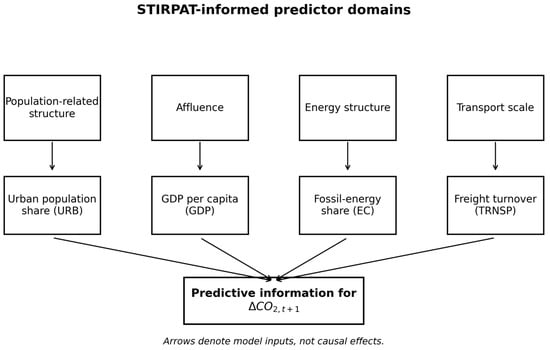
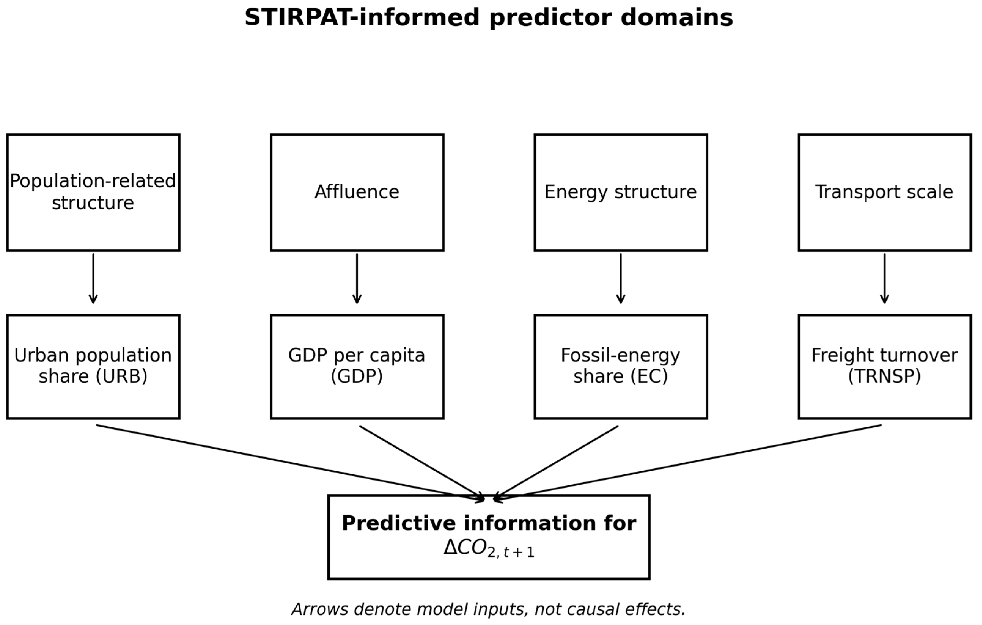
The empirical framework is informed by STIRPAT but is explicitly predictive. The urban population share represents population-related structural transformation, GDP per capita represents affluence, the fossil-energy share represents the carbon intensity of the broader energy system, and freight turnover represents physical transport activity. These domains are used to construct a parsimonious predictor set suitable for the available annual sample. Arrows in the conceptual framework therefore denote model inputs and not causal pathways.

In its conventional stochastic form, STIRPAT can be represented as I = aP^bA^cT^d e, where I denotes environmental impact, P denotes population-related pressure, A denotes affluence, T denotes technology, a is a scale parameter, b, c, and d are elasticities, and e is a disturbance term [9,10]. The present study does not estimate this multiplicative equation directly. Instead, it uses the P-A-T domains to discipline variable selection for a forecasting problem. The urban population share represents population concentration and urban structural change; GDP per capita represents affluence; the fossil-energy share represents the carbon orientation of the wider energy system; and freight turnover represents the physical scale of goods movement.

This mapping is intentionally parsimonious because the annual sample is short. Adding many highly trending national predictors would increase dimensionality, multicollinearity, and overfitting risk without guaranteeing additional forecast information. At the same time, parsimony imposes substantive limits. Passenger turnover, vehicle ownership, modal shares, transport-sector fuel use, EV penetration, road capacity, and network congestion are not explicitly represented. The framework therefore describes the information available to the forecasting models rather than a complete causal theory of China’s transport emissions. The resulting STIRPAT-informed conceptual framework is presented in Figure 1.

Figure 1. STIRPAT-informed conceptual framework. Arrows represent predictive inputs rather than causal effects.

3.2. Data Sources, Sample Period, and Variable Operationalization

The study uses annual observations for China covering 1990–2024. The outcome is the World Bank World Development Indicators series ‘Carbon dioxide (CO₂) emissions from Transport (Energy) (Mt CO₂e)’, indicator EN.GHG.CO2.TR.MT.CE.AR5, which is sourced from the EDGAR Community GHG Database. GDP per capita is obtained from WDI indicator NY.GDP.PCAP.CD. The urban population share and energy composition are taken from the National Bureau of Statistics of China (NBS). The fossil-energy share is calculated as the sum of coal, petroleum, and natural gas shares of total energy consumption. Physical transport activity is measured using NBS total freight ton-kilometers in units of 100 million ton-km. Public-source metadata were verified and retrieved on 23 September 2026.

The data audit was treated as part of the empirical methodology because forecasting results are highly sensitive to variable definitions in a sample of this size. Series were checked against their official statistical descriptions, year coverage, and units before alignment. The urbanization measure is the share of the population living in urban areas rather than an annual urban-growth rate. The fossil-energy share is reconstructed from the official shares of coal, petroleum, and natural gas in total energy consumption, thereby avoiding long blocks of mechanically imputed values. Freight activity is represented by total freight ton-kilometers, a physical work measure that combines the quantity moved with distance and is therefore more informative for national transport activity than an undocumented index.

The final 1990–2024 emissions outcome is combined with predictors dated t to construct next-year targets. Because the 2024 target is predicted using 2023 predictor information, the absence of a verified 2024 freight observation does not prevent the evaluation of the 2024 emissions outcome. This timing convention is consistent with a genuine forecasting use case: the analyst observes socioeconomic and transport information for the current year and produces a forecast for the next annual emissions realization.

During data preparation, each source series was verified against its stated statistical definition. Urbanization was operationalized as the urban population share, the fossil-energy share was reconstructed from official coal, petroleum, and natural gas shares, and transport activity was represented by physical freight turnover. Missing or placeholder values were treated as unavailable rather than as observed zeros, and no long-span mean imputation was used. The final variable definitions and source documentation are summarized in Table 3.

Table 3. Final variable definitions and source documentation.

Variable	Code	Operational Definition	Unit	Source/Identifier
Transport CO2 emissions	CO2	Carbon dioxide emissions from Transport (Energy)	Mt CO2e	WDI/EDGAR; EN.GHG.CO2.TR.MT.CE.AR5
GDP per capita	GDP	GDP per capita, current prices	Current US$	WDI; NY.GDP.PCAP.CD
Urbanization	URB	Urban population/total population	%	China NBS; Population and Its Composition
Fossil-energy share	EC	Coal + petroleum + natural gas share of total energy consumption	%	China NBS; Total Energy Consumption and Its Composition
Freight activity	TRNSP	Total freight turnover	100 million ton-km	China NBS; Freight Ton-Kilometers

3.3. Forecast-Target Construction

The study is formulated as a genuine one-year-ahead forecasting problem. Predictor information observed in year t is used to forecast transportation-related CO₂ emissions in year t + 1. The predictor vector is:

$$X_t={\left[GD{P}_t,|UR{B}_t,|E{C}_t,|TRNS{P}_t\right]}^{\prime }.$$

(1)

Rather than fitting the strongly trending emissions level directly, the models forecast the annual change:

Forecasting the annual change serves two purposes. First, it reduces the tendency of all models to obtain an apparently strong fit simply by learning the common upward level trend. Second, it creates a direct comparison with the naïve persistence benchmark, for which the implied forecast change is zero. The evaluation is nevertheless conducted after reconstructing the emissions level, so the reported RMSE and MAE remain interpretable in Mt CO₂e rather than in standardized or differenced units.

$$\Delta C{O}_{2,t+1}=C{O}_{2,t+1}-C{O}_{2,t}.$$

(2)

The predicted level is then reconstructed as:

$${\widehat{CO}}_{2,t+1}=C{O}_{2,t}+{\widehat{\Delta CO}}_{2,t+1}.$$

(3)

This alignment yields 34 one-year-ahead predictor–target pairs from 1990→1991 through 2023→2024. It also permits the 2024 outcome to be evaluated without requiring 2024 freight turnover as an input.

3.4. Temporal Validation and Leakage Prevention

The principal evaluation covers target years 2010–2024, producing 15 genuine out-of-sample forecasts. At each target year T, the estimation sample contains only observations with target years earlier than T. The training window is then expanded by one observation, and the next unseen year is forecast. All preprocessing parameters are estimated inside the relevant training period. SVR and LSTM inputs are standardized using training-only means and standard deviations; XGBoost is fitted to the original scales. No global normalization is performed before temporal splitting.

Let T denote a forecast target year. At origin T − 1, every transformation, hyperparameter decision permitted by the design, and model fit is based exclusively on observations whose target dates precede T. The training set then expands when the realized T outcome becomes available. This procedure produces a sequence of genuinely out-of-sample errors e_t = y_t − $\hat{\mathrm{y}}$_t that are directly comparable across models because each model forecasts the same target years. The use of 2010 as the first evaluation target preserves a meaningful pre-evaluation history for model fitting while still yielding 15 common forecast origins for statistical comparison.

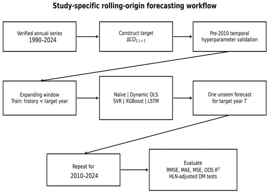
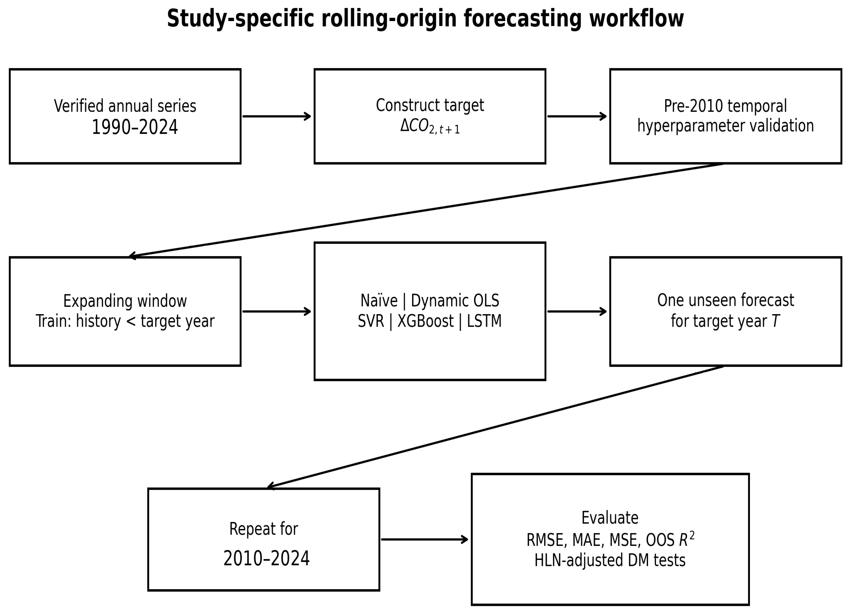
Scaling is model-specific. SVR and LSTM are sensitive to the numerical scale of inputs, so means and standard deviations are estimated only from the current training window and subsequently applied to the held-out predictor vector. XGBoost is based on tree splits and therefore does not require standardization. The target transformation for SVR and LSTM is similarly estimated within the training window and inverse-transformed before the annual change is added back to the latest observed emissions level. These steps prevent full-sample preprocessing from leaking information about the future distribution into earlier forecasts. The expanding-window forecasting and evaluation procedure is illustrated in Figure 2.

Figure 2. Study-specific expanding-window forecasting, evaluation, and interpretation workflow.

3.4.1. Naïve and Dynamic Benchmarks

The naïve persistence benchmark sets the next-year emissions level equal to the latest observed level:

$${\widehat{CO}}_{2,t+1}=C{O}_{2,t}.$$

(4)

The naïve benchmark is deliberately simple: it assumes that the best forecast of next year’s level is the most recently observed level. Such a benchmark is important for persistent environmental series because a sophisticated model should demonstrate that its predictor information adds value beyond inertia. The dynamic OLS benchmark adds a modest amount of structure by combining the latest observed annual emissions change with the same predictor vector used by the nonlinear models. It is estimated recursively at each origin and is interpreted only as a predictive regression.

The dynamic OLS specification is not used to infer causal elasticities. The regressors are national macro variables with strong common trends, the sample is short, and the equation is optimized for forecast comparison rather than structural identification. Consequently, the coefficients are not used to claim the effect of a hypothetical one-unit intervention in GDP, urbanization, the energy share, or freight activity. Its role is to provide a transparent linear-dynamic benchmark against which additional algorithmic complexity can be judged.

$$\Delta C{O}_{2,t+1}=\alpha +\varphi \Delta C{O}_{2,t}+{\mathsf{\beta }}^{\prime }{X}_t+{\epsilon }_{t+1}.$$

(5)

The dynamic specification is used as a forecasting benchmark rather than as a causal structural model.

3.4.2. Support Vector Regression

SVR constructs a regularized regression function with an ε-insensitive loss and an RBF kernel that permits nonlinear relationships between the predictors and the annual emissions change [23]. Predictors and the training target are standardized within each training window, and forecasts are inverse-transformed to the original emissions-change scale.

For training observations (x_i, y_i), SVR seeks a function f(x) = w′φ(x) + b that is as flat as possible while tolerating deviations within an ε-insensitive tube. The primal optimization minimizes model complexity and penalized slack:

$$\underset{\mathrm{w},\hspace{0.17em}b,\hspace{0.17em}\mathsf{\xi },\hspace{0.17em}{\mathsf{\xi }}^{*}}{\mathrm{m}\mathrm{i}\mathrm{n}}{\displaystyle \frac{1}{2}}\parallel \mathrm{w}{\parallel }_2^2+C{\displaystyle \sum _{i=1}^n}\left({\xi }_i+{\xi }_i^{*}\right)$$

(6)

subject to the ε-insensitive constraints:

$$\begin{array}{cc}\hfill y_i-\left[{\mathrm{w}}^{\top }\varphi \left(x_i\right)+b\right]& \le \epsilon +{\xi }_i,\hfill \\ \hfill \left[{\mathrm{w}}^{\top }\varphi \left(x_i\right)+b\right]-y_i& \le \epsilon +{\xi }_i^{*},\hfill \\ \hfill {\xi }_i,\hspace{0.17em}{\xi }_i^{*}& \ge 0,\hspace{1em}\hspace{1em}i=1,\dots ,n.\hfill \end{array}$$

(7)

$$K\left(x_i,x_j\right)=\mathrm{e}\mathrm{x}\mathrm{p}\left[-\gamma \parallel x_i-x_j{\parallel }_2^2\right]$$

(8)

Here C controls the penalty for deviations outside the ε-tube, ξ_i and ξ_i* are non-negative slack variables, and γ controls the width of the radial basis function (RBF) kernel. The formulation follows the standard ε-SVR objective [22,23].

3.4.3. Extreme Gradient Boosting

XGBoost is an ensemble tree method in which sequential regression trees are fitted to reduce prediction error while regularization constrains model complexity [25]. Shallow trees and a limited number of boosting rounds are used because the annual sample is small.

At boosting iteration m, a new regression tree f_m is added to the existing prediction to reduce a regularized objective:

$${\mathcal{L}}^{\left(m\right)}={\displaystyle {\sum }_{i=1}^n}\mathcal{l}\left[y_i,\hspace{0.17em}{\widehat{y}}_i^{\left(m-1\right)}+f_m\left(x_i\right)\right]+\Omega \left(f_m\right).$$

(9)

where l(·) is the squared-error loss and the tree-complexity penalty is:

$$\Omega \left(f_m\right)={\gamma }_{\mathrm{t}\mathrm{r}\mathrm{e}\mathrm{e}}{T}_m+{\displaystyle \frac{\lambda }{2}}{\displaystyle {\sum }_{j=1}^{T_m}}{w}_j^2.$$

(10)

Tₘ is the number of leaves in tree m, w_j is the score assigned to leaf j, λ controls L2 regularization of leaf weights, and γ_tree penalizes additional leaves. In the implemented model, max_depth, min_child_weight, subsampling, and the number of boosting rounds provide additional complexity control [25].

3.4.4. Long Short-Term Memory

The LSTM is included as a standard sequence-learning benchmark rather than as a newly proposed neural architecture [29]. Each timestep represents an actual year. To preserve sample size, the look-back length is fixed a priori at two years, so the model maps [X_t−1, X_t] to ΔCO_2t+1. The final network contains one LSTM layer with 16 hidden units, a dropout of 0.20, and a single dense output. The architecture is deliberately compact to reduce overfitting risk in the short annual sample.

For each forecast origin, the recurrent input consists of the two most recent annual predictor vectors, so the input tensor has the conceptual form [samples, look-back, features] with look-back = 2 and four features at each timestep. The network transforms this sequence into a single forecast of ΔCO_2(t+1). This is materially different from treating the four predictor columns as four timesteps; each timestep in the final design corresponds to a calendar year. The compact architecture limits parameter count while dropout and pre-evaluation validation provide additional regularization. Because the study does not modify the LSTM cell itself, no architectural novelty is claimed.

For completeness, the standard LSTM state transition used by the library implementation is:

$$f_t=\sigma \left(W_f\left[h_{t-1},x_t\right]+b_f\right),$$

(11)

$$i_t=\sigma \left(W_i\left[h_{t-1},x_t\right]+b_i\right),$$

(12)

$${\tilde{c}}_t=\mathrm{t}\mathrm{a}\mathrm{n}\mathrm{h}\left(W_c\left[h_{t-1},x_t\right]+b_c\right),$$

(13)

$$c_t=f_t\odot c_{t-1}+i_t\odot {\tilde{c}}_t,$$

(14)

$$o_t=\sigma \left(W_o\left[h_{t-1},x_t\right]+b_o\right),$$

(15)

$$h_t=o_t\odot \mathrm{t}\mathrm{a}\mathrm{n}\mathrm{h}\left(c_t\right).$$

(16)

Here x_t is the standardized predictor vector at year t, h_t is the hidden state, c_t is the cell state, f_t, i_t, and o_t are the forget, input, and output gates, σ is the logistic function, and ⊙ denotes element-wise multiplication. These equations describe the standard LSTM cell; no new cell architecture is proposed in this study [29].

3.5. Hyperparameter Selection and Reproducibility

Hyperparameters are selected before the 2010–2024 evaluation period using temporally ordered validation over pre-2010 data. For SVR, a restricted grid covers C ∈ {0.1, 1, 10, 100}, ε ∈ {0.01, 0.05, 0.10, 0.20}, and γ ∈ {scale, 0.01, 0.10, 1}. For XGBoost, the search covers 50–200 trees, maximum depths 1–3, learning rates 0.01–0.10, and subsample fractions of 0.8 or 1.0, with regularization retained. For the LSTM, the two-year look-back is fixed to preserve observations, and the tuning stage compares 4, 8, and 16 hidden units, dropout rates 0–0.20, and learning rates 0.001 and 0.005. The tuning stage uses a maximum of 200 epochs with early-stopping patience of 25; the best validation epoch is then fixed for the rolling evaluation.

The tuning philosophy is intentionally conservative. Candidate grids are restricted to ranges that are plausible for a dataset of this size, and selection occurs on temporally ordered pre-2010 validation rather than standard random k-fold cross-validation. Once the model specification is selected, it is held fixed throughout the 2010–2024 rolling evaluation. This separation between tuning and final evaluation prevents repeated adaptation to the same 15 target years. For the stochastic LSTM, five predetermined seeds are then used only as a robustness diagnostic, not to select the best realization ex post. The final model specifications used in the rolling-origin evaluation are summarized in Table 4.

Table 4. Final model specifications used in the rolling-origin evaluation.

Model	Final Specification
SVR	RBF kernel; C = 1; ε = 0.10; γ = 1.0; training-window standardization of X and target.
XGBoost	n_estimators = 50; max_depth = 2; learning_rate = 0.03; subsample = 0.8; colsample_bytree = 1.0; min_child_weight = 1; reg_lambda = 1; random_state = 42.
LSTM	look-back = 2 years; 1 LSTM layer; 16 hidden units; dropout = 0.20; Adam; learning rate = 0.005; batch size = 4; 4 fixed evaluation epochs selected in pre-2010 validation.

The analysis was implemented in Python 3.13.5 using NumPy 2.3.5, pandas 2.2.3, scikit-learn 1.8.0, XGBoost 3.1.3, statsmodels 0.14.6, SHAP 0.50.0, and PyTorch 2.10.0+cpu. Fixed seeds are used for stochastic estimation, and LSTM robustness is additionally evaluated across five predetermined seeds. A reproducibility package accompanies the manuscript with the cleaned dataset, source metadata, model scripts, forecast outputs, statistical tests, and figure/table-generation code.

3.6. Forecast Evaluation and Statistical Comparison

Forecast accuracy is evaluated on reconstructed CO₂ levels using RMSE, MAE, MSE, and out-of-sample R². RMSE is treated as the primary magnitude-sensitive criterion and MAE as a complementary robust error measure. Out-of-sample R² is reported descriptively because it can be unstable in short evaluation windows.

For the common out-of-sample evaluation targets, let e_t = y_t − $\hat{\mathrm{y}}$_t. Forecast accuracy is summarized by:

$$\mathrm{R}\mathrm{M}\mathrm{S}\mathrm{E}=\sqrt{{\displaystyle \frac{{\displaystyle {\sum }_{t=1}^n}{e}_t^2}{n}}}$$

(17)

$$\mathrm{M}\mathrm{A}\mathrm{E}={\displaystyle \frac{{\displaystyle {\sum }_{t=1}^n}\left|e_t\right|}{n}}$$

(18)

$$\mathrm{M}\mathrm{S}\mathrm{E}={\displaystyle \frac{{\displaystyle {\sum }_{t=1}^n}{e}_t^2}{n}}$$

(19)

$$R_{\mathrm{O}\mathrm{O}\mathrm{S}}^2=1-{\displaystyle \frac{{\displaystyle {\sum }_{t=1}^n}{(y_t-\widehat{y_t})}^2}{{\displaystyle {\sum }_{t=1}^n}{(y_t-\overline{\mathrm{y}})}^2}}$$

(20)

The R²_OOS value is calculated from the common out-of-sample predictions relative to the evaluation-period mean $\overline{\mathrm{y}}$. It is reported descriptively because the evaluation sample is short; RMSE and MAE are the principal forecast-error criteria.

For models A and B, define the loss differential at target t as:

$$d_t=\mathrm{L}\left(e_{A,t}\right)-\mathrm{L}\left(e_{B,t}\right),e_{k,t}=y_t-\widehat{y_{k,t}}$$

(21)

$$\mathrm{D}\mathrm{M}={\displaystyle \frac{\overline{d}}{\sqrt{\hat{\mathrm{V}}\left(\overline{d}\right)}}}$$

(22)

$$\hat{\mathrm{V}}\left(\overline{d}\right)={\displaystyle \frac{{\hat{\gamma }}_0+2{\displaystyle {\sum }_{k=1}^{h-1}}{\hat{\gamma }}_k}{n}}$$

(23)

$${\mathrm{D}\mathrm{M}}_{\mathrm{H}\mathrm{L}\mathrm{N}}=\mathrm{D}\mathrm{M}\times \sqrt{{\displaystyle \frac{\mathrm{n}+1-2\mathrm{h}+\frac{\mathrm{h}(\mathrm{h}-1)}{n}}{n}}}$$

(24)

Here $\overline{\mathrm{d}}$ is the mean loss differential and ${\hat{\mathsf{\gamma }}}_k$ is the sample autocovariance of d_t at lag k. Squared loss L(e) = e² and absolute loss L(e) = |e| are tested separately. The Harvey–Leybourne–Newbold (HLN) correction is used because the evaluation sample is small, and the corrected statistic is evaluated using a t distribution with n − 1 degrees of freedom. For the direct two-year horizon (h = 2), the variance includes the lag-1 autocovariance induced by overlapping forecast errors [26,30]. The forecast-evaluation metrics are summarized in Table 5.

Table 5. Forecast-evaluation metrics.

Metric	Definition	Interpretation
RMSE	√[(1/n)Σ(yt − $\hat{\mathrm{y}}$t)2]	Lower values indicate smaller forecast errors; large errors receive greater weight.
MAE	(1/n)Σ|yt − $\hat{\mathrm{y}}$t|	Lower values indicate smaller average absolute errors.
MSE	(1/n)Σ(yt − $\hat{\mathrm{y}}$t)2	Squared-error measure used for descriptive comparison and DM loss.
OOS R2	1 − Σ(yt − $\hat{\mathrm{y}}$t)2/Σ(yt − $\overline{\mathrm{y}}$)2	Describes fit over the evaluation period; interpreted cautiously for small n.

A non-significant DM p-value is interpreted as insufficient evidence of a difference in predictive accuracy, not as proof that two models are equivalent.

3.7. SHAP and Sensitivity Analysis

SHAP is applied to the rolling-origin XGBoost forecasts to characterize predictive attribution [28]. One genuinely out-of-sample SHAP explanation is obtained at each of the 15 forecast origins and aggregated using mean absolute SHAP values. The resulting importance measures are interpreted as contributions to the fitted prediction function rather than causal effects. Conditional sensitivity tests additionally perturb the fossil-energy share and freight activity by 5–15% while holding the remaining inputs at their reference values. These perturbations are treated as model-sensitivity diagnostics, not causal policy counterfactuals.

For feature j at forecast origin t, let φ_j,t denote its SHAP contribution to the predicted annual emissions change. Global out-of-sample importance is summarized as:

$$I_j={\displaystyle \frac{1}{n}}{\displaystyle \sum _{t=1}^n}\left|{\varphi }_{j,t}\right|.$$

(25)

The aggregation uses only the 15 held-out forecast explanations. Thus, I_j measures predictive attribution within the fitted XGBoost models and is not a causal coefficient.

For the direct two-year robustness experiment, the target is defined analogously as the cumulative change from year t to t + 2:

$${\Delta }_{2}C{O}_{2,t+2}=C{O}_{2,t+2}-C{O}_{2,t}.$$

(26)

$${\widehat{CO}}_{2,t+2}=C{O}_{2,t}+\widehat{{\Delta }_{2}C{O}_{2,t+2}}.$$

(27)

The h = 2 models are estimated directly for this two-year target rather than by iterating the one-year forecast twice.

4. Results

4.1. One-Year-Ahead Forecasting Performance

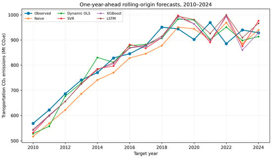
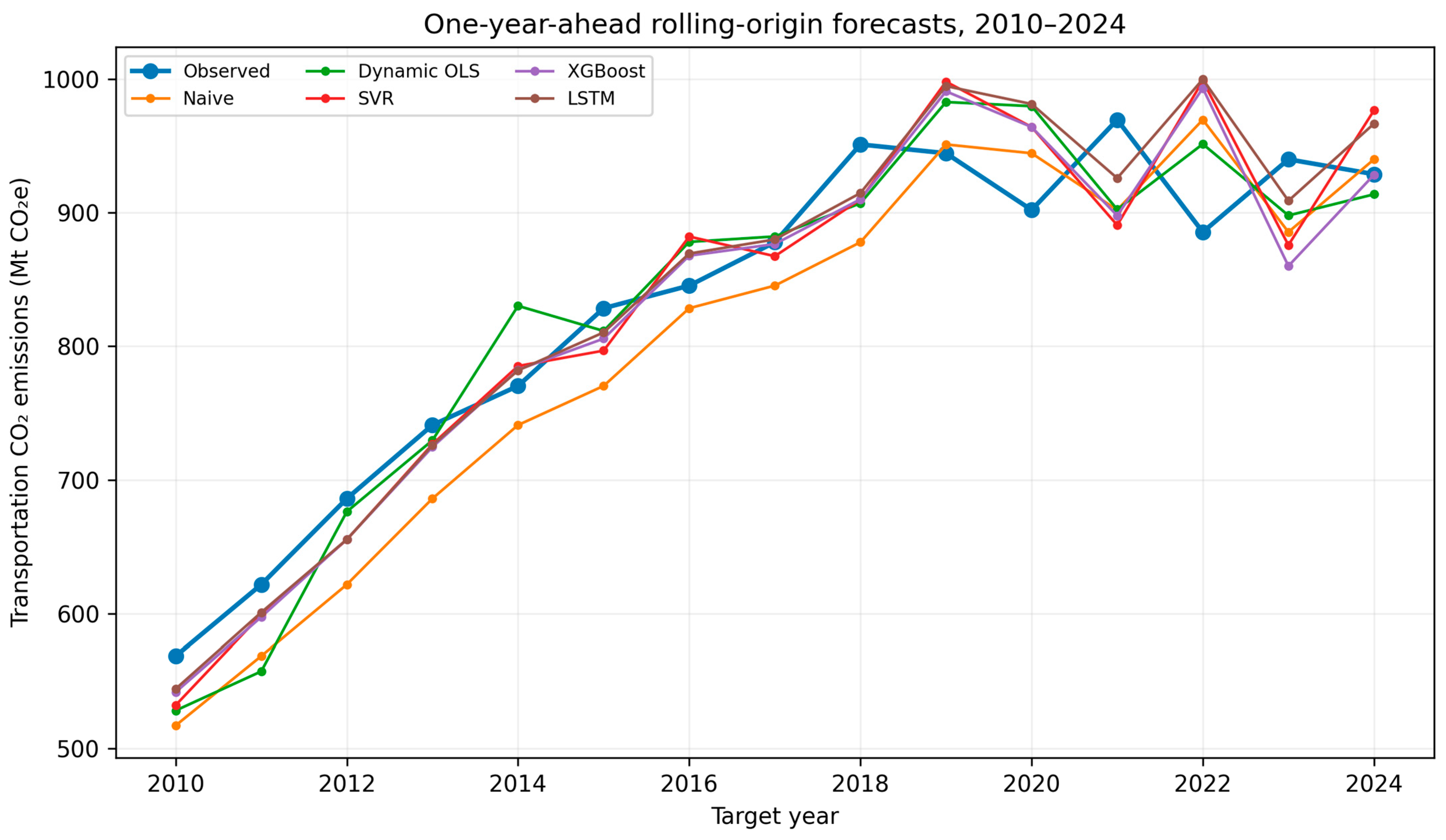
Table 6 reports the 15 common rolling-origin forecasts for 2010–2024. The LSTM records the lowest observed RMSE (45.254), MAE (35.956), and MSE (2047.882), while the dynamic OLS benchmark is close in RMSE (45.645) and XGBoost is close in MAE (37.694). SVR and naïve persistence produce larger errors. Under chronological evaluation, the performance differences among the leading models are modest, so numerical rankings should be interpreted together with the statistical comparison tests.

Table 6. One-year-ahead rolling-origin forecasting performance, 2010–2024.

Model	n	RMSE	MAE	MSE	OOS R2
Naive	15	51.705	46.660	2673.383	0.821
Dynamic OLS	15	45.645	39.336	2083.466	0.860
SVR	15	51.310	43.889	2632.680	0.823
XGBoost	15	47.914	37.694	2295.783	0.846
LSTM	15	45.254	35.956	2047.882	0.863

Note. OOS R² is calculated relative to the evaluation-period mean, as defined in Equation (20).

The closeness of the leading one-year results is substantively important. The LSTM RMSE of 45.254 Mt CO₂e is only slightly below the dynamic OLS value of 45.645, and its MAE of 35.956 is only modestly below the XGBoost value of 37.694. Therefore, the table provides no basis for treating deep learning as categorically superior. Instead, it shows that the compact recurrent model, the linear-dynamic benchmark, and the boosted-tree model all extract useful information from the short annual series, while the ranking varies with the error criterion.

The naïve benchmark is weaker than the three leading models but remains informative because its RMSE of 51.705 indicates substantial persistence in the emissions level. SVR produces a similar RMSE to the naïve benchmark but a somewhat lower MAE, suggesting that its errors are distributed differently. These patterns illustrate why multiple loss functions are useful: RMSE gives more weight to a small number of large misses, whereas MAE summarizes the typical absolute deviation.

The observed and predicted transportation-related CO₂ emissions are shown in Figure 3.

Figure 3. Observed and one-year-ahead predicted transportation-related CO₂ emissions during the 2010–2024 rolling-origin evaluation period. Each prediction uses only information available before the target year.

4.2. Forecast-Accuracy Significance Tests

The DM tests do not support a broad claim that one model is statistically superior to all alternatives. In particular, the LSTM–XGBoost comparison is not significant under squared loss (p = 0.617) or absolute loss (p = 0.725), and the dynamic OLS–LSTM comparison is also non-significant. At the conventional unadjusted 5% level, the only significant result among the reported comparisons shown in Table 7 is SVR versus LSTM under absolute loss (p = 0.034), favoring LSTM in that specific loss comparison. Given the number of pairwise comparisons, this isolated result should be interpreted cautiously. Numerical model rankings should therefore be interpreted together with the limited statistical power of 15 annual forecasts.

Table 7. HLN-adjusted Diebold–Mariano tests for one-year-ahead forecasts.

Comparison	Loss	Adjusted DM	p-Value	Interpretation
Naive vs. LSTM	Squared error	0.813	0.430	Not significant at 5%
Naive vs. LSTM	Absolute error	1.359	0.196	Not significant at 5%
Dynamic OLS vs. LSTM	Squared error	0.048	0.962	Not significant at 5%
Dynamic OLS vs. LSTM	Absolute error	0.528	0.606	Not significant at 5%
SVR vs. LSTM	Squared error	1.499	0.156	Not significant at 5%
SVR vs. LSTM	Absolute error	2.348	0.034	Significant at unadjusted 5% level
XGBoost vs. LSTM	Squared error	0.512	0.617	Not significant at 5%
XGBoost vs. LSTM	Absolute error	0.358	0.725	Not significant at 5%
SVR vs. XGBoost	Squared error	1.349	0.199	Not significant at 5%
SVR vs. XGBoost	Absolute error	1.788	0.095	Not significant at 5%
Dynamic OLS vs. XGBoost	Squared error	−0.300	0.769	Not significant at 5%
Dynamic OLS vs. XGBoost	Absolute error	0.260	0.799	Not significant at 5%

Note. The reported pairwise p-values are unadjusted for multiple comparisons. The isolated p = 0.034 result should therefore be interpreted cautiously.

The statistical tests qualify the descriptive ranking. The LSTM-XGBoost loss differentials are small relative to their year-to-year variability, yielding p = 0.617 under squared loss and p = 0.725 under absolute loss. Dynamic OLS and LSTM are even closer under squared loss (p = 0.962). The significant SVR-LSTM result under absolute loss (p = 0.034) indicates evidence of a difference for that specific pairing and loss function, but it should not be generalized to all comparisons. With only 15 forecast origins, power is limited, so non-significance should be read as insufficient evidence of superiority rather than as proof that the models are equivalent.

This distinction directly affects the study’s central conclusion. A ranking table answers which model happened to obtain the smallest error over the observed evaluation period; a forecast-comparison test asks whether the loss advantage is systematic enough to reject equal predictive accuracy. Both pieces of information are useful, but they answer different questions. Reporting them together prevents a small numerical improvement from being presented as a robust statistical result.

4.3. Forecast-Horizon and LSTM Robustness

The direct two-year-ahead experiment changes the descriptive ranking. XGBoost records the lowest RMSE (45.537) and MAE (34.426), followed by SVR in RMSE and MAE terms, while the LSTM is less competitive than at the one-year horizon. Thus, no single architecture dominates both horizons. Pairwise two-year DM tests likewise do not reject equal predictive accuracy at the 5% level for the principal model comparisons.

At h = 2, XGBoost achieves RMSE 45.537 and MAE 34.426, while the LSTM deteriorates to an RMSE of 51.892 and an MAE of 38.972. Dynamic OLS also loses ground relative to the nonlinear models. The shift suggests that information useful for the immediate next-year change is not necessarily the same as information that supports a direct two-year forecast. Shallow boosting may be better able to exploit stable threshold and interaction patterns at the longer horizon, whereas the recurrent model’s short sequence representation offers less advantage once uncertainty accumulates.

LSTM seed robustness provides a different type of evidence. Across five predetermined seeds, the mean one-year RMSE is 45.470 with a standard deviation of 0.639, the mean MAE is 35.798 ± 0.278, and the mean OOS R² is 0.861 ± 0.004. The small dispersion indicates that the compact network is not obtaining its one-year performance from a single favorable initialization. However, initialization stability is not the same as model dominance: the horizon experiment still shows that another architecture can become descriptively stronger under a different forecasting task.

The one- and two-year-ahead forecasting results are summarized in Table 8.

Table 8. Forecast-horizon robustness: one-year- and two-year-ahead accuracy.

Model	h = 1 RMSE	h = 1 MAE	h = 2 RMSE	h = 2 MAE	h = 2 OOS R2
Naive	51.705	46.660	76.243	68.978	0.610
Dynamic OLS	45.645	39.336	56.168	49.151	0.788
SVR	51.310	43.889	47.119	37.289	0.851
XGBoost	47.914	37.694	45.537	34.426	0.861
LSTM	45.254	35.956	51.892	38.972	0.819

LSTM sensitivity to stochastic initialization is limited under the compact specification. Across five predetermined seeds, the one-year RMSE averages 45.470 with a standard deviation of 0.639, MAE averages 35.798 ± 0.278, and OOS R² averages 0.861 ± 0.004. This stability is reassuring, but it does not establish universal superiority because the longer horizon ranking shifts toward XGBoost.

4.4. SHAP-Based Interpretation

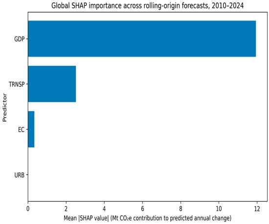
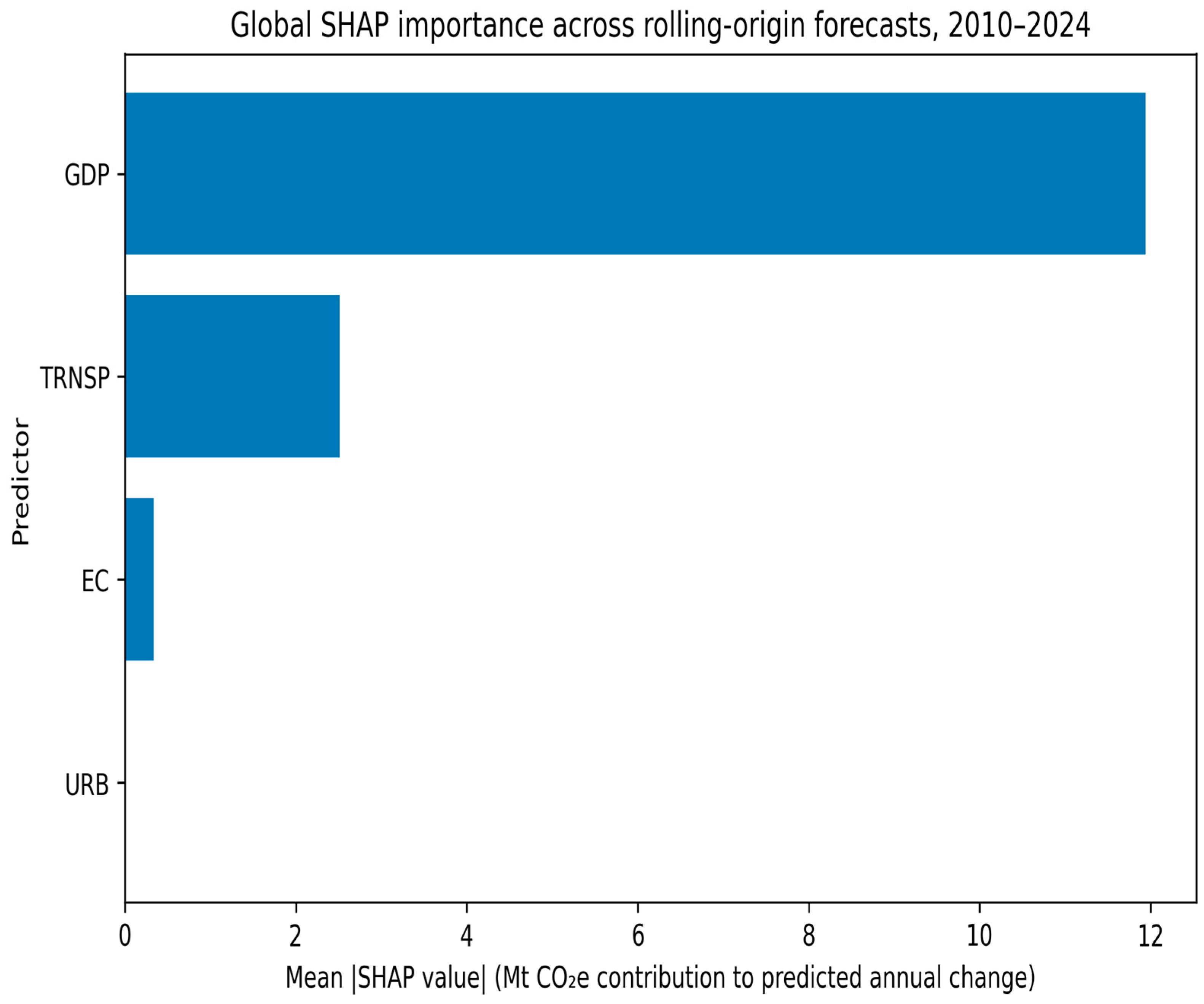
Global SHAP values are aggregated across the 15 out-of-sample XGBoost forecasts. GDP has the largest mean absolute SHAP value (11.939), followed by freight activity (2.512), the fossil-energy share (0.338), and urbanization (approximately 0 in the fitted shallow trees). These values explain which features the rolling XGBoost models use most strongly; they do not rank causal importance. Because the predictors share strong historical trends, attribution can be concentrated on one correlated variable while another receives little incremental importance.

The mean absolute SHAP value of 11.939 for GDP is several times larger than those of freight activity (2.512) and the fossil-energy share (0.338). This indicates that, within the fitted shallow XGBoost models, movements in GDP contain the largest amount of incremental information used to adjust the predicted annual change away from the model baseline. Freight activity provides a smaller but visible contribution. Urbanization receives approximately zero mean absolute attribution because the trees rarely use it after considering the other predictors.

The ranking should not be read as a substantive ranking of what ‘causes’ transportation emissions. GDP, urbanization, freight activity, and energy structure all evolve over time and are interrelated. In a small sample, a tree can select one variable as the preferred split and thereby absorb information that might otherwise be shared with correlated predictors. The result is therefore best understood as a description of the forecast function rather than an environmental impact decomposition. The global SHAP importance results are presented in Figure 4.

Figure 4. Global SHAP importance across 15 rolling-origin out-of-sample XGBoost forecasts. Bars represent mean absolute SHAP values for contributions to predicted annual emissions change; values are predictive attributions rather than causal effects.

4.5. Conditional Scenario Sensitivity

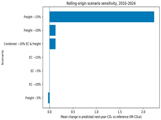
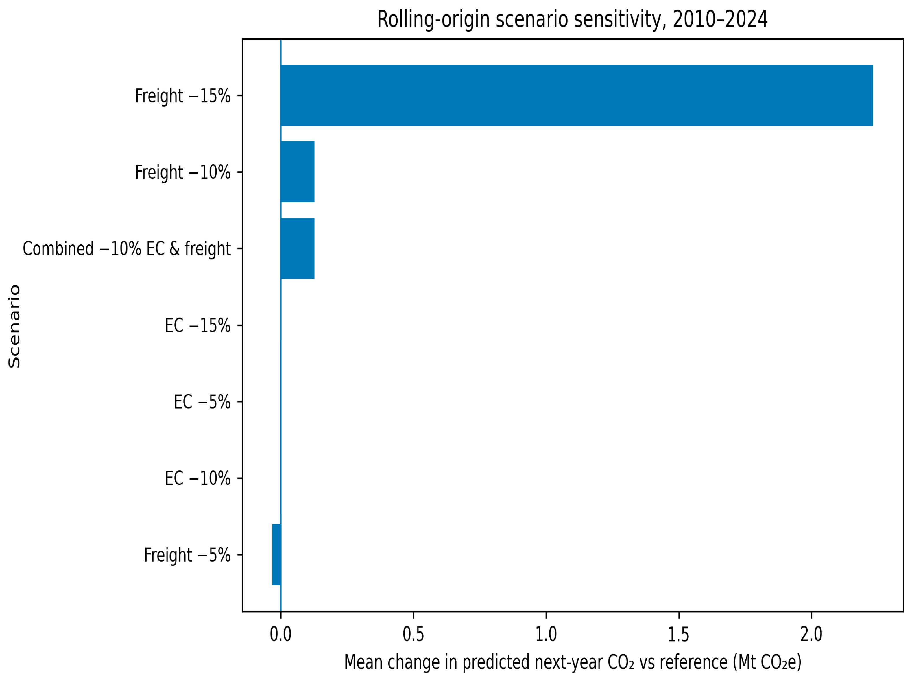
Conditional perturbations reveal limited structural sensitivity in the fitted XGBoost model. Reductions of 5–15% in the fossil-energy share do not change the rolling forecasts, while freight perturbations affect only a small subset of forecast origins and do not produce a stable monotonic emissions response. For the 2024 target, all tested perturbations leave the prediction unchanged. This behavior is consistent with the piecewise constant structure of shallow trees and the limited information content of a short annual series. The scenario exercise is therefore interpreted as a diagnostic of model responsiveness rather than a causal policy simulation.

The lack of a monotonic response is itself informative about the model scope. Because shallow regression trees are piecewise constant, moderate perturbations can leave an observation in the same terminal leaves and therefore leave the forecast unchanged. Larger freight perturbations occasionally cross split thresholds, producing discrete changes that are not proportional to the size of the perturbation. This behavior is appropriate for a sensitivity diagnostic but inappropriate for estimating intervention elasticities. The exercise therefore supports the decision not to attach numerical policy effects to unobserved mechanisms such as EV uptake, road capacity, modal substitution, or shared mobility. The conditional sensitivity results are presented in Figure 5.

Figure 5. Conditional sensitivity of rolling-origin XGBoost forecasts to changes in fossil-energy share and freight activity relative to the baseline forecast.

5. Discussion

The analysis provides a cautious account of model performance. The LSTM has the lowest observed one-year errors, but its advantage over XGBoost and dynamic OLS is modest and not statistically significant in the principal pairwise tests. At the two-year horizon, XGBoost becomes the strongest descriptive performer. The central result is therefore not that a recurrent architecture is universally superior; it is that model rankings depend on the forecast horizon, loss function, and validation design.

The first implication is that evaluation design can alter the apparent narrative of model superiority. In a short trending series, a flexible model can achieve an excellent fit under a random or single split while still providing uncertain evidence about future-year generalization. The rolling-origin design is harder because the model repeatedly faces a genuinely later observation. Under this design, the gap among the LSTM, dynamic OLS, and XGBoost becomes relatively small at h = 1, and the ordering changes at h = 2. This result is consistent with the broader forecasting principle that no architecture should be presumed superior independently of horizon, loss function, data frequency, and information set.

The strong performance of dynamic OLS deserves particular attention. It suggests that annual transport emissions retain a meaningful linear-dynamic component after the target is expressed as a year-to-year change. This does not negate a nonlinear structure; rather, it shows that nonlinear algorithms must earn their complexity by outperforming a transparent benchmark. The finding complements the China transport literature, where econometric, decomposition, and panel methods have continued to reveal interpretable relationships among economic development, urbanization, energy use, and transport activity [1,3,12].

The competitiveness of dynamic OLS is particularly informative. Recent emissions research has increasingly emphasized nonlinear and deep learning methods, but the present results show that a parsimonious dynamic specification can remain highly competitive when the sample is short. This supports a pluralistic model-comparison strategy in which conventional and flexible algorithms are evaluated under identical temporal conditions rather than treating greater algorithmic complexity as an automatic improvement.

The horizon-dependent advantage of XGBoost also aligns with the idea that tree ensembles and recurrent networks exploit different structures. XGBoost represents nonlinearities through recursive partitions and interactions; it does not require a long sequence history and can remain effective when the relationship between current predictors and a future change is threshold-like. The LSTM, by contrast, is designed to learn temporal state from ordered sequences. With only two annual timesteps and a very small training sample, its theoretical capacity is intentionally constrained. The fact that it remains competitive at h = 1 is useful evidence, but the two-year result cautions against interpreting this as a general advantage of recurrence.

This interpretation differs from studies conducted with much larger or richer datasets. Ref. [18] demonstrated the potential of ML and DL models for China transport-emissions prediction, while ref. [20] used hundreds of city-level features and observations to obtain strong predictive performance and SHAP-based interpretation. Fine-scale studies such as [7,8] incorporate route, land-use, network, or vehicle information unavailable in a national annual series. Differences in sample size and feature richness mean that model complexity that is reasonable in those settings may be inappropriate here.

The DM analysis reinforces this interpretation. Most pairwise comparisons do not reject equal predictive accuracy at the 5% level. One SVR–LSTM absolute-loss comparison is significant, but this isolated result does not justify a universal ranking. The statistical evidence is therefore weaker than the numerical metric table alone might suggest, particularly because only 15 common annual forecast origins are available.

The SHAP results answer RQ3 in predictive rather than causal terms. GDP receives the largest incremental attribution in the XGBoost forecasts, with freight activity contributing less and the fossil-energy share only modestly. Urbanization receives almost no incremental tree-based attribution after the other correlated predictors are included. This does not imply that urbanization or energy structure are substantively irrelevant; it reflects the allocation of predictive information among strongly trending variables.

From a theoretical perspective, the SHAP allocation should be interpreted alongside STIRPAT rather than as a replacement for it. STIRPAT motivates why population-related structure, affluence, and technology/energy conditions belong in the candidate information set. SHAP then describes which of the measured variables the fitted XGBoost model uses most strongly for prediction. The two frameworks operate at different levels: one organizes substantive domains, while the other explains a model’s predictive allocation. This separation prevents an algorithm-specific importance score from being presented as an estimated structural elasticity.

GDP’s dominant predictive attribution is nevertheless consistent with a broad body of China transport research that links economic scale and income growth to transport demand and emissions [1,3,12]. Freight activity’s smaller attribution is also compatible with freight-specific evidence showing that physical goods movement contributes to transport carbon outcomes [6,7]. By contrast, the near-zero incremental urbanization attribution demonstrates the limitations of interpreting correlated national trends in a tree model: it should not be used to contradict panel studies that identify urban-form or urbanization relationships under different designs and levels of aggregation.

The sensitivity analysis also delineates the limits of the present framework. Cleaner transport energy, electrification, public transport, freight-efficiency improvements, land-use coordination, and shared mobility are important mechanisms in the broader decarbonization literature, but the annual national forecasting model does not identify their causal effects. EV penetration, road capacity, vehicle ownership, passenger turnover, and modal substitution are not directly represented in the predictor set. Quantitative intervention analysis would therefore require mechanism-specific data and a structural, system-dynamics, agent-based, traffic-flow, or other suitable causal/scenario framework.

The policy interpretation therefore has to remain conditional. The model can help planners anticipate annual emissions using readily available macro indicators, and the comparison shows that simple benchmarks should be retained in operational forecasting systems. It cannot determine the causal emissions reduction from a specified EV share, an additional kilometer of road capacity, a modal shift from road to rail, or a shared-mobility program. Those questions require models with explicit behavioral, technological, or network mechanisms. System dynamics can represent feedback and adoption pathways, while agent-based and traffic-flow models can represent heterogeneous vehicles, users, and congestion processes [15,17].

Within those limits, the broader transport-decarbonization literature points to several policy domains that deserve attention: reducing the carbon intensity of transport energy, improving freight efficiency, expanding effective public transport, coordinating land use with mobility demand, and supporting low-carbon vehicle technology. Regional evidence also suggests that the same intervention may have different implications across Chinese regions because transport structures and development stages differ [2,4,6]. The present national forecasting results therefore support monitoring and planning, while intervention design should rely on more disaggregated causal and scenario evidence.

These findings inform the study’s theoretical interpretation. STIRPAT remains useful as a principled way to organize predictor domains, but the machine learning results should not be read as a formal test of STIRPAT elasticities. Likewise, the one-year LSTM result does not prove nonlinear path dependence. The more defensible inference is that both temporal persistence and nonlinear predictor relationships may contain useful forecast information, while their relative value varies across model class and forecast horizon.

5.1. Answers to the Research Questions

RQ1: The theory-informed indicators contain useful predictive information for next-year transportation CO₂ emissions. Their incremental contribution is uneven, and the common trends among GDP, urbanization, energy structure, and freight activity constrain structural interpretation.

RQ2: The LSTM records the lowest observed one-year RMSE and MAE, whereas XGBoost records the lowest two-year RMSE and MAE. Dynamic OLS is highly competitive at the one-year horizon. Most pairwise DM comparisons are not significant at the 5% level, so no model can be described as universally dominant across horizons and loss functions.

RQ3: Within the rolling XGBoost forecasts, GDP receives the largest mean absolute SHAP attribution, followed by freight activity and the fossil-energy share. These are predictive attributions rather than causal rankings, and strong collinearity requires cautious interpretation.

5.2. Practical and Policy Implications

The practical implication is methodological as much as substantive. Forecasting systems used for transport planning should preserve temporal ordering, compare against simple benchmarks, and report uncertainty around apparent performance differences. The present analysis indicates that macroeconomic and freight information are useful for forecasting, but it does not establish that manipulating any one predictor will produce a proportional change in emissions. Policy mechanisms such as cleaner energy, electrification, public transport, freight efficiency, and shared mobility should therefore be evaluated with data and models designed for causal or structural policy analysis rather than inferred directly from SHAP values or tree perturbations.

5.3. Limitations and Future Research

Several limitations define the scope of the conclusions. First, the analysis uses a short annual national time series, which limits statistical power and the complexity that can be reliably supported. Second, national predictors cannot capture detailed mechanisms involving passenger mobility, vehicle technology, EV penetration, modal choice, congestion, road capacity, or infrastructure. Third, strong temporal collinearity complicates feature attribution. Fourth, SHAP explains fitted predictions rather than causal effects, and the scenario exercise is diagnostic rather than counterfactual. Finally, the findings are specific to the available national annual dataset. Future work should use higher-frequency and spatially disaggregated data, direct passenger and freight measures, vehicle stock, EV share, transport-energy consumption, modal composition, and infrastructure variables. Such data would also enable credible system-dynamics, agent-based, traffic-flow, and physics-informed models.

A further limitation is that annual aggregation conceals within-year volatility and structural breaks. Higher-frequency monthly or quarterly transport-energy, freight, vehicle, and mobility indicators could provide many more observations and allow richer lag structures. Provincial or city-level panels would additionally support the analysis of spatial heterogeneity and would make it possible to compare national aggregate forecasts with geographically disaggregated models.

Future research should therefore proceed in two directions. The first is predictive: expand the information set with passenger turnover, vehicle stock, modal shares, transport-specific energy use, EV penetration, logistics efficiency, and infrastructure variables; evaluate additional transparent benchmarks such as ARIMAX or regularized dynamic regression; and test models over multiple rolling windows and forecast horizons. The second is structural: connect the forecast evidence to system-dynamics, agent-based, traffic-flow, or physics-informed models once the corresponding mechanism-specific data are available. These extensions would permit policy scenarios to be evaluated without asking a purely predictive model to answer causal questions it was not designed to identify.

6. Conclusions

This study examined transportation-related CO₂ emissions in China using annual data for 1990–2024 within a theory-informed comparative forecasting framework. The design uses verified predictor definitions, genuine one-year-ahead alignment, chronological expanding-window evaluation, training-only preprocessing, pre-evaluation hyperparameter selection, conventional benchmarks, forecast-comparison tests, SHAP interpretation, and robustness analyses.

The primary one-year-ahead experiment shows that the compact LSTM records the lowest observed RMSE and MAE, but the advantage over dynamic OLS and XGBoost is modest and is not statistically significant in their direct pairwise comparisons. At the two-year horizon, XGBoost records the lowest RMSE and MAE. The evidence therefore does not support a claim that either deep learning or machine learning is universally superior for this short annual series.

Global SHAP analysis shows that GDP contributes the largest share of incremental predictive information to the rolling XGBoost forecasts, followed by freight activity and the fossil-energy share. These attributions describe the fitted prediction function and should not be interpreted as causal effects. Conditional scenario tests likewise show that the present model is not sufficiently structurally sensitive to quantify intervention-specific policy effects.

Overall, the main contribution is methodological: rigorous temporal validation and conventional benchmarks materially change the conclusions that would be drawn from a random or single-split analysis. For small annual emissions datasets, model complexity should be justified by demonstrated out-of-sample gains rather than assumed from architecture alone. Future research using higher frequency and mechanism-specific transport data can connect this forecasting framework with richer structural and simulation approaches for policy analysis.

Substantively, the study also demonstrates the value of combining theory and predictive evaluation without conflating them. STIRPAT-informed domains provide a defensible basis for choosing a small set of national predictors, while the rolling-origin experiment determines how much forecasting value those variables provide across competing model classes. SHAP helps describe the fitted nonlinear model, but the accompanying sensitivity analysis shows why model explanation should not be turned into causal policy simulation. This separation of forecasting, interpretation, and intervention analysis is especially important when the available sample is short and the predictors share strong historical trends.

For journal readers and practitioners, the practical message is therefore conservative but useful: employ verified data definitions, preserve temporal order, compare sophisticated algorithms with simple dynamic benchmarks, report both numerical and statistical forecast evidence, and test whether conclusions persist across horizons. Under those conditions, complex models can be evaluated on demonstrated predictive value rather than on architectural reputation. For China’s transport sector, richer high-frequency and disaggregated data will be necessary before forecasting models can be linked credibly to detailed intervention scenarios involving electrification, modal substitution, congestion, infrastructure, and shared mobility.

References

- Yang, W.; Li, T.; Cao, X. Examining the Impacts of Socio-Economic Factors, Urban Form and Transportation Development on CO2 Emissions from Transportation in China: A Panel Data Analysis of China’s Provinces. Habitat Int. 2015, 49, 212–220. [Google Scholar] [CrossRef] [Scilit]
- Gao, X.; Shao, S.; Gao, Q.; Zhang, Y.; Wang, X.; Wang, Y. Factors Influencing Carbon Emissions and Low-Carbon Paths in China’s Transportation Industry. Energy 2025, 323, 135778. [Google Scholar] [CrossRef] [Scilit]
- Li, Y.; Du, Q.; Lu, X.; Wu, J.; Han, X. Relationship between the Development and CO2 Emissions of Transport Sector in China. Transp. Res. Part Transp. Environ. 2019, 74, 1–14. [Google Scholar] [CrossRef] [Scilit]
- Guo, B.; Geng, Y.; Franke, B.; Hao, H.; Liu, Y.; Chiu, A. Uncovering China’s Transport CO2 Emission Patterns at the Regional Level. Energy Policy 2014, 74, 134–146. [Google Scholar] [CrossRef] [Scilit]
- Lin, B.; Du, Z. How China’s Urbanization Impacts Transport Energy Consumption in the Face of Income Disparity. Renew. Sustain. Energy Rev. 2015, 52, 1693–1701. [Google Scholar] [CrossRef] [Scilit]
- Lv, Q.; Liu, H.; Yang, D.; Liu, H. Effects of Urbanization on Freight Transport Carbon Emissions in China: Common Characteristics and Regional Disparity. J. Clean. Prod. 2019, 211, 481–489. [Google Scholar] [CrossRef] [Scilit]
- Zhao, P.; Li, Z.; Xiao, Z.; Jiang, S.; He, Z.; Zhang, M. Spatiotemporal Characteristics and Driving Factors of CO2 Emissions from Road Freight Transportation. Transp. Res. Part Transp. Environ. 2023, 125, 103983. [Google Scholar] [CrossRef] [Scilit]
- Zhu, B.; Hu, S.; Chen, X.M.; Roncoli, C.; Lee, D.-H. Uncovering Driving Factors and Spatiotemporal Patterns of Urban Passenger Car CO2 Emissions: A Case Study in Hangzhou, China. Appl. Energy 2024, 375, 124094. [Google Scholar] [CrossRef] [Scilit]
- Dietz, T.; Rosa, E.A. Rethinking the Environmental Impacts of Population, Affluence and Technology. Hum. Ecol. Rev. 1994, 1, 277–300. [Google Scholar]
- York, R.; Rosa, E.A.; Dietz, T. STIRPAT, IPAT and ImPACT: Analytic Tools for Unpacking the Driving Forces of Environmental Impacts. Ecol. Econ. 2003, 46, 351–365. [Google Scholar] [CrossRef] [Scilit]
- Ehrlich, P.R.; Holdren, J.P. Impact of Population Growth: Complacency Concerning This Component of Man’s Predicament Is Unjustified and Counterproductive. Science 1971, 171, 1212–1217. [Google Scholar] [PubMed]
- Lin, B.; Xie, C. Reduction Potential of CO2 Emissions in China׳ s Transport Industry. Renew. Sustain. Energy Rev. 2014, 33, 689–700. [Google Scholar] [CrossRef] [Scilit]
- Cao, P.; Liu, Z.; Zhang, H.; Wei, L. The Impact of Agglomeration on CO2 Emissions in China’s Transport Sector: A Spatial Econometric Analysis. Sustain. Cities Soc. 2024, 117, 105966. [Google Scholar] [CrossRef] [Scilit]
- Zuo, D.; Zhao, L.; Lu, Z.; Xiong, Q.; Luo, Y. Multilayer Structural Path Analysis of CO2 Emissions in China’s Transportation Sector. Transp. Res. Part Transp. Environ. 2024, 128, 104083. [Google Scholar] [CrossRef] [Scilit]
- Feng, Y.Y.; Chen, S.Q.; Zhang, L.X. System Dynamics Modeling for Urban Energy Consumption and CO2 Emissions: A Case Study of Beijing, China. Ecol. Model. 2013, 252, 44–52. [Google Scholar] [CrossRef] [Scilit]
- Li, C.; Zhang, Z.; Wang, L. Carbon Peak Forecast and Low Carbon Policy Choice of Transportation Industry in China: Scenario Prediction Based on STIRPAT Model. Environ. Sci. Pollut. Res. 2023, 30, 63250–63271. [Google Scholar] [CrossRef] [Scilit] [PubMed]
- Akopov, A.S.; Beklaryan, L.A.; Saghatelyan, A.K. Agent-Based Modelling of Interactions between Air Pollutants and Greenery Using a Case Study of Yerevan, Armenia. Environ. Model. Softw. 2019, 116, 7–25. [Google Scholar] [CrossRef] [Scilit]
- Ji, T.; Li, K.; Sun, Q.; Duan, Z. Urban Transport Emission Prediction Analysis through Machine Learning and Deep Learning Techniques. Transp. Res. Part Transp. Environ. 2024, 135, 104389. [Google Scholar] [CrossRef] [Scilit]
- Yu, W.; Xia, L.; Cao, Q. A Machine Learning Algorithm to Explore the Drivers of Carbon Emissions in Chinese Cities. Sci. Rep. 2024, 14, 23609. [Google Scholar] [CrossRef] [Scilit] [PubMed]
- Zhao, L.; He, Z. Using Machine Learning to Analyze the Factors Influencing City-Level Transportation Carbon Emissions. Energy 2025, 333, 137355. [Google Scholar] [CrossRef] [Scilit]
- Boser, B.E.; Guyon, I.M.; Vapnik, V.N. A Training Algorithm for Optimal Margin Classifiers. In Proceedings of the Fifth Annual Workshop on Computational Learning Theory; Association for Computing Machinery: New York, NY, USA, 1992; pp. 144–152. [Google Scholar]
- Cortes, C.; Vapnik, V. Support-Vector Networks. Mach. Learn. 1995, 20, 273–297. [Google Scholar] [CrossRef] [Scilit]
- Smola, A.J.; Schölkopf, B. A Tutorial on Support Vector Regression. Stat. Comput. 2004, 14, 199–222. [Google Scholar] [CrossRef] [Scilit]
- Friedman, J.H. Greedy Function Approximation: A Gradient Boosting Machine. Ann. Stat. 2001, 29, 1189–1232. [Google Scholar] [CrossRef] [Scilit]
- Chen, T.; Guestrin, C. XGBoost: A Scalable Tree Boosting System. In Proceedings of the 22nd ACM SIGKDD International Conference on Knowledge Discovery and Data Mining, San Francisco, CA, USA, 13–17 August 2016; Association for Computing Machinery: New York, NY, USA, 2016; pp. 785–794. [Google Scholar]
- Hochreite, S.; Schmidhuber, J. Long Short-Term Memory. Neural Comput. 1997, 9, 1735–1780. [Google Scholar] [CrossRef] [Scilit] [PubMed]
- Wang, X.; Su, Y.; Zheng, Z.; Wang, W. Heterogeneity Analysis of CO2 Emissions Driving Features on Road Transport: New Perspective from Interpretive Machine Learning. J. Clean. Prod. 2025, 490, 144726. [Google Scholar] [CrossRef] [Scilit]
- Lundberg, S.M.; Lee, S.-I. A Unified Approach to Interpreting Model Predictions. Adv. Neural Inf. Process. Syst. 2017, 30, 4765–4774. [Google Scholar]
- Harvey, D.; Leybourne, S.; Newbold, P. Testing the Equality of Prediction Mean Squared Errors. Int. J. Forecast. 1997, 13, 281–291. [Google Scholar] [CrossRef] [Scilit]
- Diebold, F.X.; Mariano, R.S. Comparing Predictive Accuracy. J. Bus. Econ. Stat. 2002, 20, 134–144. [Google Scholar] [CrossRef] [Scilit]
Disclaimer/Publisher’s Note: The statements, opinions and data contained in all publications are solely those of the individual author(s) and contributor(s) and not of MDPI and/or the editor(s). MDPI and/or the editor(s) disclaim responsibility for any injury to people or property resulting from any ideas, methods, instructions or products referred to in the content. |
© 2026 by the authors. Licensee MDPI, Basel, Switzerland. This article is an open access article distributed under the terms and conditions of the Creative Commons Attribution (CC BY) license.