Environmental Ratings and Subsequent Reported Emissions Intensity: A Layered Validity Test in China and Korea

Abstract

Environmental ratings combine corporate policies and performance, but their interpretation depends on the criterion, horizon and reporting boundary. We apply a four-layer validity framework to a retrospectively reconstructed 2014–2025 panel of 209 Chinese and 115 Korean listed firms selected based on data coverage. Fixed-effects models estimate within-firm associations. In the common 2019–2023 exposure window, none of the 12 country-specific or between-country associations with next-year emissions intensity survives Benjamini–Hochberg adjustment (minimum q = 0.920). Two- and three-year associations emerge in the extended history; their statistical classification depends on temporal support and the finite sample covariance correction. Ratings converge with selected Chinese climate action and disclosure assessments. Korean measurement agreement is strongly boundary-dependent: excluding four firms with documentary-supported scope mismatches raises log-scale concordance between provider and regulatory emissions from 0.734 to 0.989 across 142 remaining pairs from 18 firms. Recent reports directly document particular years rather than every historical boundary. This study contributes a validation protocol linking each claim to its criterion, temporal support, organizational scope and precision. These results guide the joint use of ratings and emissions evidence without attributing causal effects or establishing equivalence to zero.

1. Introduction

Environmental ratings inform capital allocation, regulatory accountability and corporate governance. Their inputs include policies, targets, disclosure, management systems and reported outcomes. These components may respond at different speeds: reporting can improve before capital replacement reduces emissions. The relevant empirical question is therefore which environmental criterion a rating tracks, over what horizon and within which reporting boundary.

Prior research first documented uncertainty within environmental, social and governance (ESG) ratings. Berg et al. [1] attribute much of the disagreement among providers to differences in measurement and scope. Avramov et al. [2] and Gibson Brandon et al. [3] show that this disagreement affects investment and pricing. Agreement among providers, however, does not show that a rating corresponds to a defined environmental outcome. Ferro et al. [4] find that inputs from the London Stock Exchange Group (LSEG) combine forward-looking aspirations with backward-looking performance. A high score is therefore not a single physical variable by construction. A review of 41 corporate climate-scoring systems reaches a related conclusion: standardized verified inputs and transparent science-based weighting remain uncommon [5].

Disclosure research suggests competing mechanisms. Better-performing firms may use precise and comparable disclosure to reduce information asymmetry [6]. Firms under legitimacy pressure may instead emphasize favorable information or omit adverse outcomes [7,8]. Neither the adoption of a reporting framework nor assurance alone guarantees substantive information quality [9,10]. Assurance is associated with less disagreement among rating providers [11], but this information-layer finding does not establish physical validity. A meta-analysis similarly shows that results depend on how disclosure and performance are measured [12].

Mandatory sustainability reporting can alter information production, but effects depend on content, enforcement, and use [13].

Direct evidence on ratings and carbon outcomes is also mixed. Studies of Chinese firms report favorable associations with carbon efficiency or environmental performance [14,15], whereas evidence from the airline industry indicates weak capture or prediction of emissions [16]. Park et al. [17] use a 2011–2017 difference-in-differences design around the first phase of the Korean Emissions Trading Scheme. They report no statistically significant reduction in emissions among covered listed firms relative to non-covered controls, even as Korean Corporate Governance Service environmental ratings increased. Vendor estimates, disclosure choices, and scaling decisions can also alter capital-market inferences [18]. Different criteria, entity boundaries, coverage rules, and inferential methods can therefore produce different conclusions [19].

Three measurement problems motivate a joint validation design. First, a relative fiscal label such as FY0 can refer to different calendar years for ratings, emissions and financial fields. We use t for the calendar year assigned from each field’s period end date and t + h for an outcome h calendar years later. Second, unequal country histories change the firm–years available for comparison. Third, action indices, accountability ranks and emissions records represent distinct criteria and organizational scopes. Field date alignment, common temporal support and boundary-specific agreement are therefore part of substantive validity assessment [20].

China and Korea provide complementary institutional settings for this assessment. The Corporate Climate Action Transparency Index (CATI) measures action and disclosure in China; the Institute of Public & Environmental Affairs (IPE) provides retrieval-time environmental accountability information. Korea’s Greenhouse Gas Inventory and Research Center (GIR) supplies verified emissions for a restricted matched subset. The analysis applies a common rating model across countries and preserves the distinct meaning of each external criterion.

We ask three research questions. RQ1: Is within-firm variation in environmental-pillar or emissions scores associated with subsequent emissions-to-revenue intensity, and how does this association vary over one to three years? RQ2: How do the country-specific slopes and their directly estimated difference change with temporal support? RQ3: Which information/action, accountability and regulatory criteria support convergence or agreement? These are conditional associations in a retrospective provider history.

The distinctive contribution is a layered criterion-validity test of ratings, emissions and regulatory verification under common temporal support and explicit organizational-boundary constraints. First, field-level reconstruction makes the timing of unlike vendor fields auditable. Second, identical-support horizon comparisons separate changes in follow-up length from changes in baseline sample composition. Third, the regulatory comparison quantifies how much apparent disagreement changes after documented scope mismatches are excluded. This design turns a general question about rating usefulness into specific decisions about criteria, horizons and permissible data combinations.

2. Theory and Layered Validity Framework

2.1. Environmental Ratings as Composite Information Signals

The environmental component of an ESG rating can be useful even when it is not a direct measure of physical decarbonization. Providers aggregate policies, targets, governance systems, disclosures, controversies, and outcome indicators. These components can reduce search costs and indicate whether a firm has developed the capacity to identify and manage environmental risk. Ferro et al. [4], however, show why a composite score requires validation before it can be interpreted as a physical measure: aspirational features and realized performance enter the same rating architecture. A score can rise when commitments, reporting systems, or policies improve before emissions measurably change.

This distinction yields two competing mechanisms. Voluntary disclosure theory predicts that better environmental performers can signal their type through more complete and credible information, producing convergence between the information and physical layers [6]. Legitimacy and selective-disclosure accounts predict that firms under greater environmental pressure can strengthen positive information or governance responses even when adverse outcomes persist [7,8]. Assurance may increase the credibility of a specified disclosure, but its scope, level, and provider are endogenous and heterogeneous [10,21]. Reductions in provider disagreement associated with assurance [11] should therefore be interpreted at the information-credibility layer; they do not by themselves show that scores track later emissions.

Digital adoption is one candidate link between information systems and physical performance. Lin et al. [22] examine the heterogeneous carbon-performance implications of digital technology adoption. Digitization can strengthen monitoring and process control while also changing energy demand, so its net implication is empirical. The archived panel has no validated, consistently dated adoption measure; governance or disclosure scores are not substituted for one. Reviews of environmental disclosure and senior management and evidence on audit committees further motivate separating organizational information production from realized emissions [23,24].

2.2. A Four-Layer Validity Model

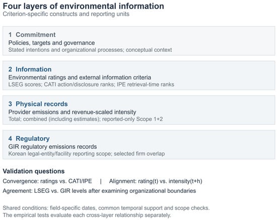
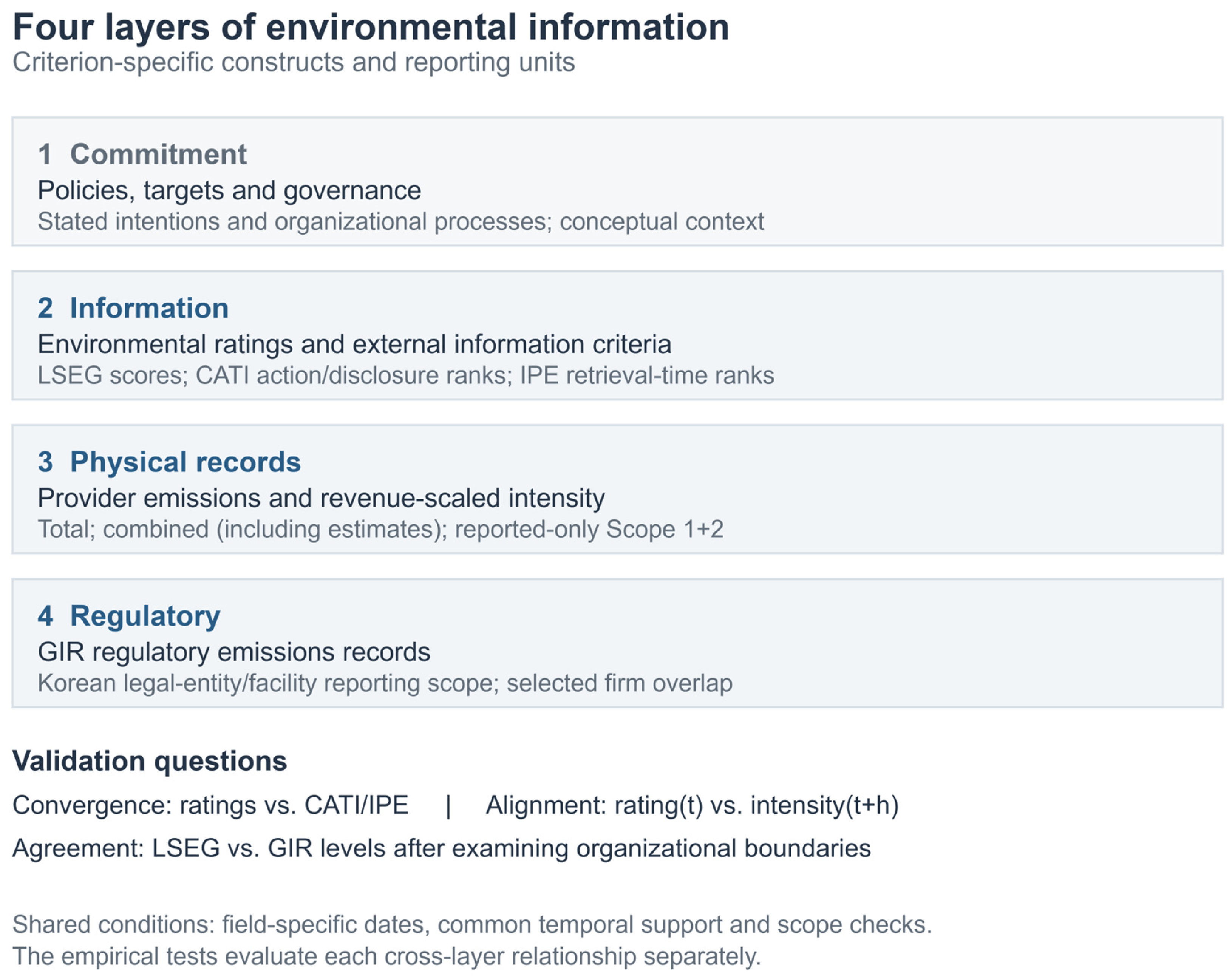
Figure 1 separates four layers. Commitments and governance provide conceptual context. The information layer includes ratings, CATI action/disclosure assessments and the IPE retrieval-time accountability rank. The physical-record layer contains provider total and combined-scope emissions, with reported/estimated status retained. The regulatory layer contains Korean GIR-verified emissions. Each comparison preserves its own construct and reporting unit; IPE accountability is not regulator-verified emissions.

Figure 1. Layered validity framework for environmental ratings. Note. The four panels distinguish constructs and reporting units; the validation questions specify the comparisons conducted. CATI denotes Corporate Climate Action Transparency Index; IPE, Institute of Public & Environmental Affairs; GIR, Greenhouse Gas Inventory and Research Center. Combined Scopes 1 + 2 can include provider estimates; the strict-reported sensitivity requires both reported components.

The framework links each research question to a testable comparison. RQ1 evaluates the physical criterion associations of scores with future intensity at explicitly stated horizons. RQ2 estimates the Korea-minus-China slope directly under a common specification and period. RQ3 distinguishes construct convergence with action/disclosure ranks from agreement between emissions measures. Competing signaling and legitimacy mechanisms permit positive, negative or weak conditional associations, which motivates two-sided tests rather than a uniformly directional hypothesis.

The practical output is a criterion-specific evidence profile. Construct convergence supports information screening; emissions associations concern a defined outcome and horizon; source substitution additionally requires acceptable level agreement and verified reporting scope. Each test therefore informs a different use of environmental information.

2.3. Cross-Institutional Comparability

Institutional differences can change both what a rating observes and what an external criterion means. China and Korea differ in terms of disclosure requirements, assurance practices, emissions-trading coverage, corporate-group structures, and legal-entity reporting. A comparison of average ratings would confound these institutional features with firm performance. We instead test whether a one-standard-deviation-higher standardized score within a firm’s country, two-digit Refinitiv Business Classification (TRBC) industry, and year is associated with the next-year outcome. We then estimate the difference between the country-specific slopes directly. This design evaluates within-industry relative validity. It cannot determine whether similarly rated firms in high- and low-impact industries have comparable absolute environmental effects, which is a separate cross-industry calibration problem [25].

The external criteria have complementary coverage: CATI assesses action and disclosure, IPE records accountability at retrieval, and GIR provides regulatory emissions. Their separate analyses identify where validation is available and where it remains incomplete. They are not combined into a national environmental ranking.

3. Materials and Methods

The analysis uses three complementary statistical components. Multiway fixed-effects panel regressions estimate within-firm rating–intensity associations and direct country-slope contrasts (Section 3.4). External validation uses Spearman rank correlations for CATI and IPE and a separate fixed-effects regression for the GIR criterion (Section 3.5). Paired-source agreement statistics, with whole-firm bootstrap intervals, compare LSEG and GIR emissions measurements (Section 3.6). The four-layer framework organizes these distinct quantities; it is not itself a statistical estimator. Section 3.7 reports supplementary sensitivity analyses.

3.1. Sample, Temporal Scope, and Data Governance

The initial frame contained 5748 Chinese listed security records. A usable relative-fiscal-year row required both focal scores, total emissions, revenue and the four controls. At least one usable year was available for 796 Chinese organizations; the five-year eligibility rule retained 209. In Korea, 3029 security records represented 2823 provider organizations; 168 had at least one usable year, and 115 met the five-year threshold. CSR-field availability removed no additional organizations, and false CSR responses were retained (Table S9). Thus, the Korean condition was an observed-field availability check, not an affirmative reporting criterion. This rule selected firms with sustained coverage before field-specific calendar reconstruction. The registry separately envisaged at least two observations for model eligibility. The archived main estimator retains complete cases without enforcing a universal two-row filter; one-row firms contribute no within-firm score variation. The five-year screen governs cohort membership, and outcome-specific missingness governs each estimation sample. The reconstructed skeleton contains 324 × 12 = 3888 firm–years during 2014–2025. Primary one-year models use exposures in 2019–2023 and outcomes through 2024; the extended exposure window begins in 2015. The target population is these coverage-screened firms and their observed histories.

Table S9 compares retained firms with firms having one to four usable years. Retained firms are larger and more highly rated in both countries: median firm-level asset summaries are USD 11.69 versus 3.57 billion in China and USD 10.78 versus 2.73 billion in Korea; corresponding environmental scores are 57.78 versus 49.64 and 64.49 versus 47.33. Emissions intensity differences do not have a uniform direction. These descriptive comparisons use the original relative-fiscal-year screening records, not a newly reconstructed panel for excluded firms, and omit firms with no usable year. Licensed firm-level data remain controlled; non-identifying aggregate results and analysis code accompany the revision.

3.2. Field-Specific Reporting Date Reconstruction

The field date audit enumerated 324 firms × 39 fields × 11 relative fiscal positions, giving 138,996 candidate field position cells. Among these, 81,052 had usable values with directly retrievable field dates and contributed dated observations. The first count describes the audit grid; the second describes usable dated values, not additional firm–years. Values without a field-specific date were excluded from calendar inference. The reconstruction used observed dates without forward filling or substituting nominal fiscal labels.

The 2014–2025 panel contains 81,052 values with direct field date support. Independent checks found no date-to-year mismatch, missing in-range dated value, extra cell, or numerical discrepancy. We also compared nine same-scope Scopes 1 + 2 firm–years for Korean Air, Samsung Electro-Mechanics, and CJ CheilJedang with company reports; all nine matched after field date alignment. Korea Electric Power Corporation was retained as a negative control because its organizational boundary differed from the available company-report boundary. Correct timing is necessary, but it cannot make unlike organizational scopes equivalent. These dates locate reporting periods, not the dates on which investors first received information. Retrospective downloads may include provider revisions and backfilling.

Three proprietary LSEG green-revenue estimate series contain 10,182 nonempty values but lack directly retrievable field dates. We exclude these series from inferential models rather than increase coverage through unverifiable dating. A directly dated environmental-products revenue field is too sparse for the main analysis and remains descriptive. These choices narrow the outcome set but preserve temporal interpretability.

3.3. Ratings, Physical Outcomes, and Financial Controls

The focal exposures are the LSEG environmental-pillar and emissions scores. To reduce differences in country, industry, and year scales, we standardize each score within country, TRBC two-digit industry, and year. When a cell contains fewer than five observations or has zero variance, the archived fallback standardizes the remaining fallback observations within country–year, rather than against the full country–year population. Both stages use population SD (ddof = 0). Of 3006 observed score records, 2855 (95.0%) were standardized within country–industry–year, and 151 (5.0%) used the country–year fallback; no observed score failed standardization. A coefficient therefore represents the conditional association with a one-standard-deviation-higher standardized score relative to firms in the same country, industry, and year. It does not represent a one-unit improvement in absolute environmental performance. The environmental pillar aggregates resource-use, emissions and innovation categories using industry materiality weights; the emissions category includes management and commitment information as well as outcomes. We use the legacy ESG Scores methodology archived in August 2026, not the separate new Sustainability Ratings product [26].

The two outcomes are natural logs of emissions divided by same-year consolidated revenue. The provider’s total CO₂-equivalent field (TR.CO₂EmissionTotal) covers direct Scope 1 plus indirect Scope 2 emissions; it does not include Scope 3. The second series separately sums the provider’s combined Scope 1 and Scope 2 fields and can include estimated values. Thus, the two outcomes differ in terms of data construction and coverage, not in the number of scopes. Revenue (TR.F.TotRevenue) was exported in USD; the regression unit is log metric tons of CO₂ equivalent per USD. Multiplying intensity by one million for descriptive presentation changes only its log constant. Logs require positive finite emissions and revenue; missing or non-positive values are excluded, not recoded as zero. A separate reviewer-added sensitivity requires both scope components to be reported (Table S19). Neither outcome is an independent verification of physical abatement.

Combined and separately reported components are not interchangeable fields: on identical strict samples, their sums are equal in 1281/1954 extended-window observations (65.6%) and 1012/1480 common-window observations (68.4%). All four component dates agree within these observations. The differences include 317 and 189 observations, respectively, with both combined components labeled Reported_value. Table S21 separates model-labeled discrepancies from these residual field differences; the exported metadata do not identify their market/location basis or record-level source priority.

Current-period controls are log USD total assets, return on assets, debt-to-assets and capital-expenditure-to-revenue; each interacts with the Korea indicator. Table S18 gives the field definitions, units and transformations. Dollar revenue can incorporate exchange-rate and revenue-composition changes, so an intensity decline is not necessarily an absolute emissions reduction. Country–year effects absorb shared annual country shocks but do not establish a constant-output or constant-currency outcome. Green-revenue fields lacking date support are excluded from the inferential models.

3.4. Within-Firm Rating Associations and Country Contrasts

The primary method is a linear panel regression estimated by least squares after absorbing multiple fixed effects. The quantity being estimated, or the estimand, is the conditional within-firm slope relating a one-unit-higher standardized rating at year t to log reported emissions-to-revenue intensity at year t + 1. We estimate the China slope, the Korea slope and their direct difference. A score unit follows the country–industry–year standardization and fallback defined in Section 3.3; it is neither a raw rating point nor one within-firm standard deviation. The specification is

Y(i,t + 1) = [β_CN + β_Diff × Korea(i)] Score(i,t) + γ′X(i,t) + δ′[X(i,t) × Korea(i)] + α(i) + λ(c,t) + θ(s,t) + ε(i,t)

Y is log emissions-to-revenue intensity; Score is the standardized environmental-pillar or emissions score; X contains the four financial controls. Korea(i) equals 1 for Korean firms and 0 for Chinese firms. Firm effects α(i), country–year effects λ(c,t) and two-digit-industry–year effects θ(s,t) are absorbed. The China slope is β_CN; the Korea slope is β_CN + β_Diff; β_Diff is the Korea-minus-China contrast. All three are tested two-sided. In the horizon extensions, t + 1 is replaced by t + h, with the rest of the specification retained.

Firm effects account for stable firm characteristics, country–year effects for annual shocks shared within each country, and industry–year effects for shared annual sector conditions. Interacting the score and each control with Korea(i) allows all five slopes to differ between countries in one pooled model. A separate country intercept is absorbed by the firm effects. The score interaction tests the country difference directly rather than inferring a difference by comparing the significance of two separately reported slopes.

China is the reference category in this expression. Replacing Korea(i) with China(i) = 1 − Korea(i) gives the equivalent score term [β_KR + β_CN−KR × China(i)] Score(i,t), where β_KR = β_CN + β_Diff and β_CN−KR = −β_Diff. The control coefficients also transform: γ_KR = γ + δ and δ_CN−KR = −δ. With the same sample and estimation settings, this changes only the parameterization: fitted values, residuals, country-specific slopes and their uncertainty remain identical. The country-difference sign reverses, its interval is reflected around zero, and its two-sided test is unchanged. Supplementary Methods S2 gives the coefficient and covariance transformation.

The firm is the independent inferential unit, and firm–years are repeated observations. We use the type 1 cluster-robust covariance estimator (CR1), clustered by firm, and set inferential degrees of freedom to the number of firm clusters minus one [27]. Fixed effects and controls address several observed and time-invariant sources of confounding, but they do not convert an observational conditional association into a causal effect of ratings.

The archived CR1 covariance multiplies the firm-cluster sandwich by G/(G − 1) × (N − 1)/(N − r), where r is the rank of the residualized slope design; absorbed-effect rank is not counted in this finite sample factor. Independent QR projection, statsmodels and PyFixest reproduce this convention. Table S22 additionally counts nonnested absorbed effects, counts the full fixed-effect rank and removes fixed-effect singleton observations. These are explicitly labeled convention sensitivities, not changes to the original analysis family.

Four primary models combine the two scores with the two provider emissions intensity outcomes. The 2019–2023 common window is primary for cross-country interpretation because both countries have joint temporal support for scores and outcomes. The 2015–2023 extended window tests sensitivity to earlier and uneven historical coverage. In each window, the four models produce China, Korea, and Korea-minus-China contrasts, yielding 12 primary tests. We apply the Benjamini–Hochberg procedure to the 12 two-sided raw p values within each window [28]. Nine non-core registered models cover resource use, commitments, target stringency, verification, assurance standards, and environmental-management systems. These models are corrected within their own prespecified families and cannot replace the primary result. We do not describe unadjusted findings as marginally significant. Supporting Methods S2 and Table S2 document the prespecified analysis families and primary-model sample flow.

3.5. External Validation Ladder

CATI assesses climate action and disclosure for Chinese listed firms in 2022 and 2023 [29,30]. Annual ranks are converted to percentiles, with higher values indicating stronger assessed performance, then compared with same-year scores using Spearman correlations. The four year-by-score comparisons form one Benjamini–Hochberg (BH) family. Positive adjusted associations in both releases provide repeated annual evidence of information/action convergence. Changing CATI versions and matched samples make these two annual cross-sections, not a balanced longitudinal replication.

The IPE record is a dynamic firm environmental-performance rank retrieved on 9 August 2026 for 208 of the 209 Chinese sample firms [31]. We link the retrieval-time percentile to the 2024 LSEG scores and use this comparison as an environmental-accountability boundary stress test. The two score correlations form one adjusted family. Because the IPE record is not a 2015–2024 firm–year panel, it cannot support claims about historical improvement and is not made mechanically symmetric with GIR.

Korea’s Greenhouse Gas Inventory and Research Center supplies regulator-verified greenhouse gas emissions for covered entities [32]. We use security codes, firm names, and the OpenDART service of Korea’s Data Analysis, Retrieval and Transfer System (DART) to link 22 listed firms to the rating data. A GIR legal-entity or facility boundary can differ from the consolidated-group boundary used by LSEG. We therefore conduct two separate analyses: score-to-GIR criterion validation and a direct LSEG-to-GIR measurement-agreement audit. One source never fills a missing value in the other.

Score-to-GIR models relate scores and controls at t to verified intensity at t + 1, absorb firm and year effects and cluster by firm. Inference uses both CR1 and a null-imposed, restricted wild-cluster bootstrap with 9999 Rademacher replications, two-sided absolute t statistics and a plus-one correction [33,34]. The base seed is 20260811 plus the deterministic model–window offset documented in the code. Within each scenario and window, the two score tests form a BH family for each inference method. The original joint robustness rule requires both adjusted q values to be below 0.05, a CR1 interval excluding zero and a consistent direction across windows. Post-review seed, replication and cluster-influence diagnostics are reported in Table S17. GIR intensity divides metric tons of CO₂ equivalent by 2015 KRW real revenue in billions from OpenDART separate financial statements [35], deflated with the World Bank GDP deflator [36]. This denominator and scope differ from primary consolidated USD intensity.

The supplementary small-cluster audit reports cluster-size quantiles, N²/Σn_g², concentration of residualized score variation and leave-one-firm-out coefficient ranges. It repeats 9999 draws at base seeds 20260811, 20261007 and 20261008, plus 4999 and 19,999 draws at the original seed. Exact model-specific seeds are in the aggregate archive. These are Monte Carlo sensitivity checks, not evidence that few-cluster uncertainty has disappeared.

The discrepancy audit identified 29 pairs outside a factor-of-two LSEG/GIR band. Twenty-eight belong to four firms with persistent group, overseas-operation or multi-entity scope differences supported by report anchors; one historical discrepancy in 2018 remains unresolved. The original four regression scenarios retain all firms, remove the 29 pairs, remove the four persistent-mismatch firms, or remove all five flagged firms. For agreement, we additionally separate removal of the 28 documentary-linked rows from removal of all 29 ratio-flagged rows. Documentary anchors cover selected recent years, not every historical firm–year. These exclusions are selected sensitivities; the ratio filter is outcome-selected, and the remaining firms have not all been positively verified as boundary-equivalent.

The documentary sensitivity excludes Korean Air, Samsung Electro-Mechanics, CJ CheilJedang and KEPCO after discrepancy screening and public-report adjudication (Table S20). It removes their complete 40-pair histories, compared with 28 documented anomalous pairs under the row-level rule. Recent-year anchors support the boundary interpretation; earlier-year exclusion is extrapolative, and the remaining 18 firms are not presumed to be positively verified as comparable. Sources include Korean Air [37], Samsung Electro-Mechanics [38], CJ CheilJedang [39,40] and KEPCO [41,42].

3.6. Agreement Statistics and Computational Quality

The agreement audit pairs provider total emissions and GIR emissions by firm and calendar year. Pearson and Spearman correlations assess co-movement; Lin concordance and ICC(A,1) assess absolute agreement on the log scale [43,44,45]. We report geometric and median LSEG/GIR ratios, descriptive Bland–Altman ratio limits and tolerance shares [46,47,48]. Point estimates are calculated from the original pooled pairs. Additional log ratio decomposition separates persistent between-firm from within-firm discrepancy variation. These descriptive components quantify source disagreement, not error relative to an observed true emissions standard.

For each of the five agreement samples, a nonparametric bootstrap draws G firms with replacement from its G observed firms, with equal selection probability. Every selected firm contributes all its paired LSEG–GIR years; a repeated selection contributes that complete history again. Each statistic is recalculated after the selected histories are pooled. This preserves the pairing of sources and dependence across years within firms. We use 9999 draws, initializing NumPy’s default random generator separately for each sample with seed 20260829. Pointwise 95% intervals are the 2.5th and 97.5th percentiles of the replicate statistics. All 9999 replicates were finite for each archived statistic. These whole-firm percentile intervals are distinct from the null-imposed wild-cluster tests for the GIR regression coefficients. Supplementary Methods S2 details the calculations, and Table S16 reports all five samples.

The original registry contains 13 model specifications fitted in two windows. Analyses requested in the preceding review cycle were added in separate dated plans before their computation, with test families separated from the original primary family. That revision independently reproduced all eight original primary fits and all sixteen GIR scenario–window–score fits from retained inputs. The aggregate audit records full-rank and convergence checks, bootstrap settings, source hashes and actual runtime versions. The added longitudinal analyses used Python 3.13.14, NumPy 2.5.1, pandas 2.3.3 and SciPy 1.18.0; boundary analyses used Python 3.12.14, NumPy 2.3.5, pandas 3.0.1 and SciPy 1.16.1. The independent covariance comparison additionally used statsmodels 0.14.6, PyFixest 0.60.0 and linearmodels 7.0. These environments refer to those retained analyses; the exact interpreter for the initial analysis was not retained. The present minor revision clarifies the existing procedures and does not introduce new original-data estimates.

OpenAI Codex assisted with English-language editing, document organization, reference formatting, code preparation and computational checks for the reviewer-requested analyses. The exact model and application-build identifiers for all sessions were not retained. Analyses used the licensed study data; no synthetic observations were used to generate the empirical findings. The authors are responsible for the accuracy, interpretation and final content of the manuscript. All numerical statements in the revision are linked to retained aggregate outputs and computational checks.

3.7. Reviewer-Requested Horizon, Directionality and Precision Analyses

Exact calendar-year joins add outcomes at t + 2 and t + 3 with the original score standardization, controls and fixed effects. Outcomes end by 2024; the extended exposure starts in 2015, and the common-coverage exposure starts in 2019. A second comparison requires all three outcomes on the same baseline rows, leaving exposure periods 2015–2021 and 2019–2021. Added available-support horizons form separate 24-contrast BH families per window; identical-support comparisons form separate 36-contrast families. The original one-year families remain unchanged. Tables S12 and S13 report all estimates and sample counts.

A one-year sensitivity adds current log intensity and its country interaction, with an unadjusted model fitted on exactly the same rows. Separate diagnostics relate current scores to prior-year intensity and report descriptive pooled and within-firm correlations. Each regression diagnostic has a separate 12-contrast BH family per window (Tables S14 and S15). The current-outcome model is a sensitivity rather than a bias-corrected dynamic estimator, because short-panel fixed-effects estimates with a lagged outcome can be biased [49]. No externally established intervention or validated instrument set is available for an event study or causal dynamic model.

Approximate 80% minimum detectable magnitudes are SE × [t(1 − alpha/2, G − 1) + Φ⁻¹(0.80)], using the achieved firm-clustered standard error and G firms. We report nominal alpha = 0.05 and a conservative Bonferroni reference of 0.05/12. These are not observed power or equivalence tests; BH has no single fixed detection threshold. Table S10 gives all twelve precision diagnostics. Table S11 separately reports raw and standardized score variation, including the within-firm share of total sum of squares.

4. Results

4.1. Field Date Reconstruction and Model Support

The field audit distinguishes 138,996 candidate cells from 81,052 usable dated values (Section 3.2). Table 1 reports the sample and calendar support, and Table S2 reports the availability in each model stage.

Table 1. Data, sample, and temporal support.

Item	Country/Window	Size	Interpretive Boundary
Coverage-screened firms	China	209	At least five usable years; not all listed firms
Coverage-screened firms	Korea	115	At least five usable years; not all listed firms
Calendar-year skeleton	Combined	3888 firm–years	324 firms × 2014–2025
Direct field date support	Combined	81,052 cells	Values with a direct LSEG period end date only
Total emissions intensity models	Extended 2015–2023	2174 firm–years; 324 firms	China 1273; Korea 901
Total emissions intensity models	Common 2019–2023	1571 firm–years; 324 firms	China 1008; Korea 563
Scopes 1 + 2 intensity models	Extended 2015–2023	2372 firm–years; 324 firms	China 1405; Korea 967
Scopes 1 + 2 intensity models	Common 2019–2023	1599 firm–years; 324 firms	China 1026; Korea 573

Note. LSEG denotes London Stock Exchange Group Data & Analytics. Firm-level LSEG values remain license-restricted. The table reports aggregate sample formation and temporal support only.

The two total emissions intensity models contain 2174 firm–years in the extended window and 1571 in the common window. The two Scopes 1 + 2 models contain 2372 and 1599 firm–years, respectively. All four models retain the same 209 Chinese and 115 Korean firms in both windows. The common window therefore does not contain a different set of firms. It is the jointly observed historical period for the same 324 firms, with fewer usable firm–years because the interval is shorter.

4.2. Common-Window Primary Estimates

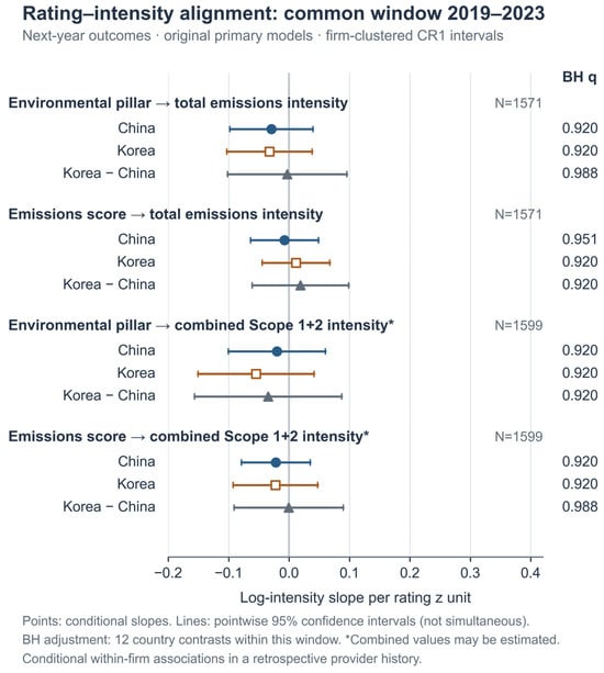
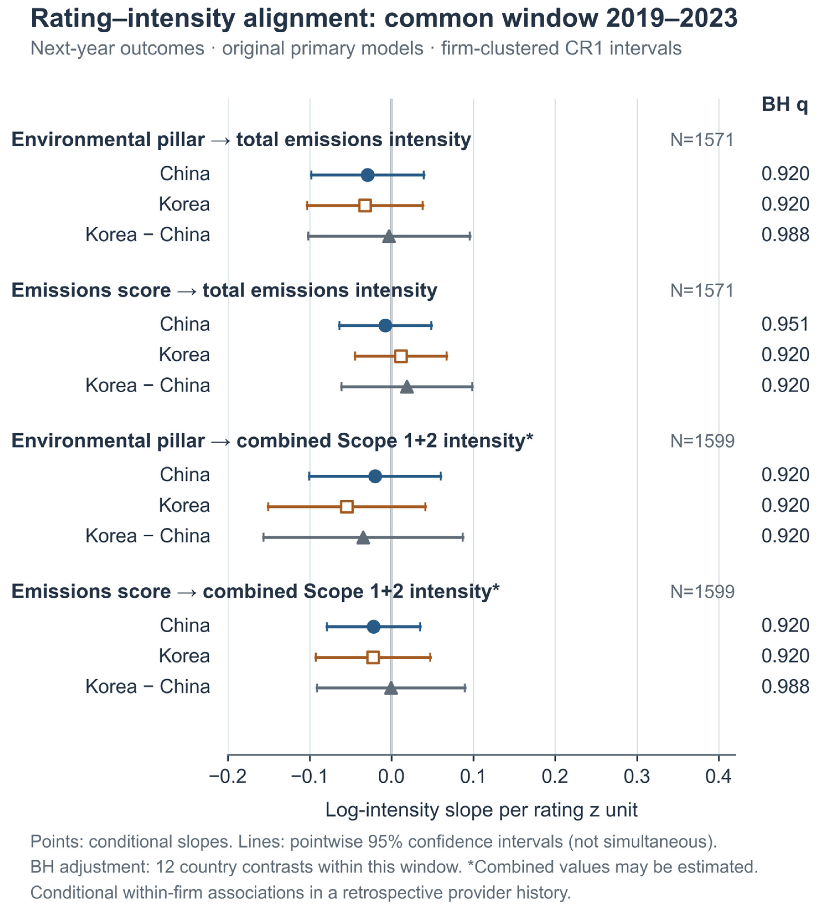
Figure 2 and Table 2 report the four primary models. For the environmental-pillar score and next-year total emissions intensity, the common-window coefficient is −0.029 in China (95% CI [−0.098, 0.039]) and −0.032 in Korea (95% CI [−0.103, 0.038]). The Korea-minus-China difference is −0.003 (95% CI [−0.102, 0.096]). All three intervals include zero; their adjusted q values are 0.920, 0.920, and 0.988. For the emissions score, the corresponding coefficients are −0.008 in China, 0.011 in Korea, and 0.019 for the country difference. None has a q below 0.920.

Figure 2. Primary common-window conditional associations. Note. Points are within-firm conditional slopes for a one-standard-deviation-higher rating; bars are firm-clustered 95% confidence intervals. SD denotes standard deviation; CI, confidence interval. Marker shape and fill distinguish China, Korea, and the Korea-minus-China difference, including when the figure is printed in grayscale. All 12 contrasts belong to the common-window Benjamini–Hochberg family. Combined Scopes 1 + 2 includes provider-estimated observations; the strict-reported sensitivity is reported separately in Table S19.

Table 2. Primary model estimates.

Score and Outcome	Window	China Beta [95% CI] (q)	Korea Beta [95% CI] (q)	Korea-Minus-China Beta [95% CI] (q)
Environmental pillar to next-year total emissions intensity	Common window, 2019–2023	−0.029 [−0.098, 0.039] (0.920)	−0.032 [−0.103, 0.038] (0.920)	−0.003 [−0.102, 0.096] (0.988)
Emissions score to next-year total emissions intensity	Common window, 2019–2023	−0.008 [−0.064, 0.049] (0.951)	0.011 [−0.045, 0.067] (0.920)	0.019 [−0.061, 0.099] (0.920)
Environmental pillar to next-year combined Scopes 1 + 2 intensity	Common window, 2019–2023	−0.020 [−0.100, 0.060] (0.920)	−0.055 [−0.151, 0.041] (0.920)	−0.035 [−0.156, 0.087] (0.920)
Emissions score to next-year combined Scopes 1 + 2 intensity	Common window, 2019–2023	−0.022 [−0.079, 0.035] (0.920)	−0.023 [−0.092, 0.047] (0.920)	−0.001 [−0.091, 0.090] (0.988)
Environmental pillar to next-year total emissions intensity	Extended window, 2015–2023	−0.101 [−0.173, −0.028] (0.059)	0.124 [−0.030, 0.278] (0.227)	0.225 [0.054, 0.395] (0.059)
Emissions score to next-year total emissions intensity	Extended window, 2015–2023	−0.037 [−0.107, 0.033] (0.440)	0.011 [−0.112, 0.133] (0.866)	0.048 [−0.094, 0.190] (0.621)
Environmental pillar to next-year combined Scopes 1 + 2 intensity	Extended window, 2015–2023	−0.102 [−0.196, −0.009] (0.096)	0.023 [−0.084, 0.129] (0.738)	0.125 [−0.018, 0.268] (0.208)
Emissions score to next-year combined Scopes 1 + 2 intensity	Extended window, 2015–2023	−0.089 [−0.165, −0.014] (0.080)	−0.051 [−0.139, 0.036] (0.429)	0.038 [−0.078, 0.154] (0.621)

Note. Common-window and extended-window results appear in separate blocks. Within each block, four score-outcome models yield 12 BH-adjusted contrasts. CI denotes a pointwise firm-clustered 95% confidence interval. Total denotes the provider’s Scopes 1 + 2 total field; combined Scopes 1 + 2 denotes the separately summed reported/estimated series. A between-country contrast is a difference in slopes, not a difference in average emissions.

The Scopes 1 + 2 models show the same pattern. Environmental-pillar coefficients are −0.020 for China, −0.055 for Korea, and −0.035 for the difference, with q = 0.920 for all three. Emissions-score coefficients are −0.022, −0.023, and −0.001, with q values of 0.920, 0.920, and 0.988, respectively. None of the 12 China, Korea, or Korea-minus-China contrasts across the four models satisfies q < 0.05; the minimum q is 0.920.

The common-window intervals quantify the substantial remaining uncertainty. For the eight country-specific slopes, the approximate 80% minimum detectable magnitudes based on achieved standard errors are 0.080–0.137 log units at nominal alpha = 0.05 and 0.106–0.182 under a conservative 12-test Bonferroni reference (Table S10). The positive-scale counterparts are 8.3–14.7% and 11.2–20.0%, respectively. These are precision diagnostics, not equivalence margins or effects ruled out by the data. For the total intensity model, the standardized environmental-score within-firm SDs are 0.556 in China and 0.467 in Korea; within-firm variation accounts for 24.5% and 17.8% of the total standardized-score sum of squares, respectively (Table S11). Ratings vary within firms, but this study remains unable to distinguish some modest associations from zero.

4.3. Extended-Window Coverage Sensitivity

4.3.1. Original Extended Window and Outcome Construction

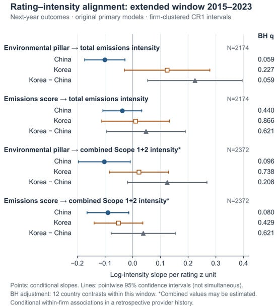
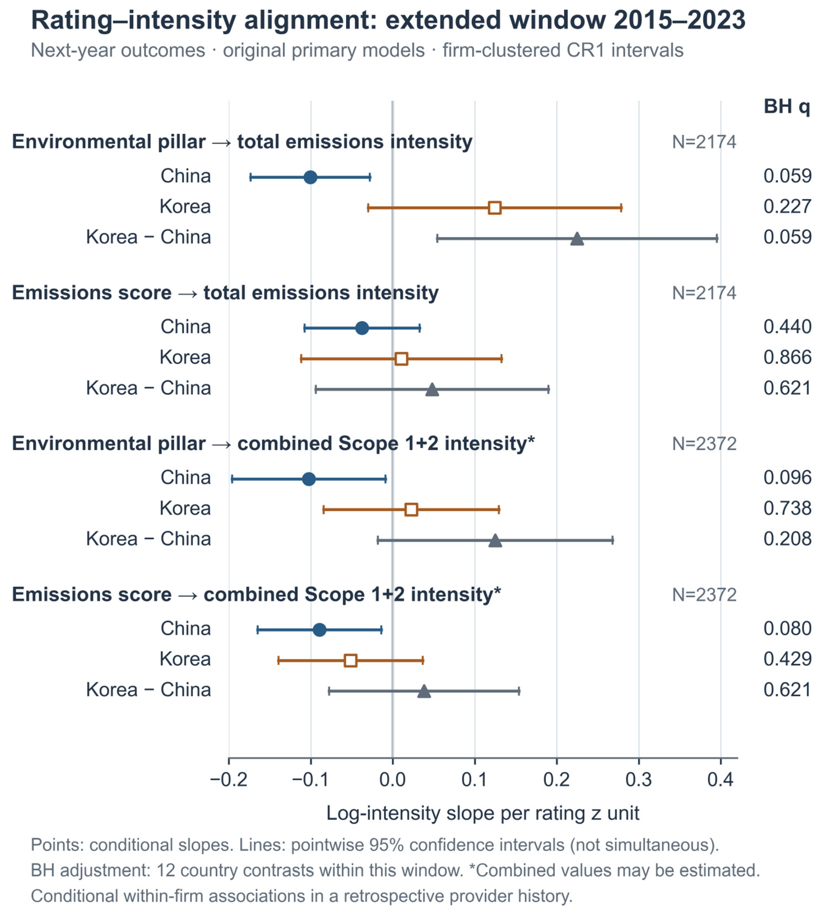
Figure 3 reports all four extended-window models; Figure 2 reports the corresponding common-window models. In China, the environmental-pillar coefficient for next-year total emissions intensity is −0.101 (95% CI [−0.173, −0.028], p = 0.0068). The Korea-minus-China contrast is 0.225 (95% CI [0.054, 0.395], p = 0.0099). Both have a q = 0.059 after adjustment. For next-year combined Scopes 1 + 2 intensity in China, the environmental-pillar and emissions-score coefficients are −0.102 and −0.089, respectively, with q = 0.096 and q = 0.080. No extended-window primary contrast has q < 0.05.

Figure 3. Extended-window conditional associations for the four primary models. Note. The plot contains only extended-window estimates, with 2015–2023 exposures and t + 1 outcomes. Corresponding common-window estimates appear in Figure 2. Bars are pointwise firm-clustered 95% confidence intervals. The two contrasts labeled adjusted p = 0.059 have the smallest BH q values; neither meets q < 0.05. This display is not a formal cross-window coefficient-difference test. Combined Scopes 1 + 2 can include estimates; the strict-reported sensitivity appears in Table S19.

The smaller common-window estimates identify historical coverage as part of the association being estimated. Firm effects do not restore missing historical periods. The following analyses separate outcome construction, follow-up horizon and temporal direction.

None of the nine non-core registered models for resource use, commitments, target stringency, verification, assurance standards, or environmental-management systems has a q < 0.05 in either window within its prespecified family. Tables S5 and S6 report the registry and all 18 model–window fits rather than a selected subset. This result applies to the measures and timing analyzed here; it does not show that the underlying arrangements have no environmental consequences.

For the strict reported Scopes 1 + 2 outcome, common-window models retain 1480 rows from 320 firms (205 China; 115 Korea); none of the six contrasts survives BH adjustment (minimum q = 0.684). In the extended window, the China environmental-pillar slope is −0.128 [−0.203, −0.054] (q = 0.005). The matched sample combined-series comparison also has an adjusted extended-window association (minimum q = 0.016), whereas the common-window minimum is 0.721 (Table S19). The outcome definition and sample restriction therefore matter jointly.

4.3.2. Longer-Horizon Associations

At the added two- and three-year horizons, eight of 24 extended-window contrasts survive BH adjustment (minimum q = 0.021). They concern environmental-pillar China slopes and Korea-minus-China contrasts for both outcomes. For total intensity, the China coefficients are −0.104 [−0.180, −0.029] at t + 2 (q = 0.025) and −0.104 [−0.183, −0.025] at t + 3 (q = 0.031). The corresponding country differences are 0.316 [0.105, 0.528] and 0.276 [0.102, 0.451], both q = 0.021. No added common-coverage contrast survives adjustment (minimum q = 0.239), although some unadjusted intervals exclude zero (Table S12).

With identical baseline rows across horizons, ten of 36 extended-window contrasts survive adjustment (minimum q = 0.029) versus none in the common-coverage comparison (minimum q = 0.325). The common identical-support models contain 917 total intensity rows from 317 firms or 951 combined-scope rows from 324 firms over 2019–2021 (Table S13). These results show sensitivity to horizon and temporal support, not a formal cross-window coefficient difference.

4.3.3. Temporal Direction and Covariance Sensitivity

Current-outcome adjustment yields no BH rejection (minimum q = 0.949 common; 0.171 extended). Reverse-temporal models do reveal three adjusted common-window associations: prior combined-scope intensity with current environmental scores in China (−0.107 [−0.185, −0.029], q = 0.043), with emissions scores in Korea (−0.240 [−0.397, −0.082], q = 0.036), and its country difference (−0.230 [−0.408, −0.051], q = 0.047). Tables S14 and S15 also report same-sample unadjusted fits and descriptive correlations. Prior emissions therefore form part of the observed rating history; temporal sequencing alone does not identify the direction of causation.

Independent covariance checks reproduce standard errors and adjusted q values to numerical precision. Counting nonnested fixed-effect degrees of freedom raises standard errors by 1.2–2.1% and retains eight added-horizon extended-window BH rejections. Counting the full absorbed-effect rank raises them by 10.1–26.1%; none of the 24 added-horizon extended-window contrasts then meets q < 0.05 (minimum q = 0.055). Fixed-effect singleton removal changes, at most, two rows and no BH decision (Table S22). The original common-window non-rejection persists under all audited conventions.

4.4. Chinese CATI and IPE Validation

Table 3 reports Chinese external validation. CATI overlaps with 54 sample firms in 2022 and 106 in 2023. Environmental-pillar scores correlate positively with the annual relative ranks: Spearman rho is 0.300 and 0.249, with q = 0.037 and 0.020, respectively. These adjusted associations provide repeated annual evidence of action/disclosure convergence in changing samples. Emissions-score correlations are 0.265 and 0.315, with q = 0.052 and 0.004, respectively. Only the 2023 emissions-score association survives adjustment.

Table 3. Chinese CATI and IPE external validation.

Criterion	Rating	Year/Match	Result	Validity Classification
CATI climate action/disclosure rank	Environmental pillar	2022 (N = 54)	rho = 0.300; q = 0.037	Repeated convergence; changing matched samples
CATI climate action/disclosure rank	Environmental pillar	2023 (N = 106)	rho = 0.249; q = 0.020	Repeated convergence; changing matched samples
CATI climate action/disclosure rank	Emissions score	2022 (N = 54)	rho = 0.265; q = 0.052	Partial convergence; 2023 only
CATI climate action/disclosure rank	Emissions score	2023 (N = 106)	rho = 0.315; q = 0.004	Partial convergence; 2023 only
IPE retrieval-time environmental rank	Environmental pillar	LSEG 2024 to IPE 2026-08-09 (N = 208)	rho = 0.020; q = 0.778	Convergence not established at the retrieval-time boundary
IPE retrieval-time environmental rank	Emissions score	LSEG 2024 to IPE 2026-08-09 (N = 208)	rho = 0.043; q = 0.778	Convergence not established at the retrieval-time boundary

Note. CATI denotes Corporate Climate Action Transparency Index; IPE, Institute of Public & Environmental Affairs; LSEG, London Stock Exchange Group Data & Analytics; N, number of matched firms; rho, Spearman rank correlation; and q, the Benjamini–Hochberg-adjusted p value. CATI evaluates an information/action construct. The IPE measure is a retrieval-time accountability rank dated 9 August 2026. Neither criterion is regulator-verified emissions.

The IPE boundary produces a different result. The correlations of the 2024 environmental-pillar and emissions scores with the IPE environmental-performance rank retrieved on 9 August 2026 are 0.020 and 0.043, respectively; both have q = 0.778. This cross-section does not establish convergence between the LSEG ratings and retrieval-time environmental accountability. Because IPE is not a historical firm–year panel, the result cannot show whether Chinese firms improved or deteriorated during 2015–2024.

Environmental-pillar convergence is observed in both CATI releases, with matched samples increasing from 54 to 106 firms. The changing coverage and index versions limit claims of longitudinal replication. The result supports an action/disclosure interpretation within those matched samples; the retrieval-time IPE rank addresses a separate accountability criterion.

4.5. Korean GIR Criterion Validation and Boundary Sensitivity

Table 4 reports the score-to-GIR estimates for 22 Korean firms. In the extended window, 191 firm–years produce an environmental-pillar coefficient of 0.037 (95% CI [−0.095, 0.169]) and an emissions-score coefficient of −0.029 (95% CI [−0.091, 0.033]). Both CR1-adjusted q values are 0.565, and both wild-cluster q values are 0.687. In the common window, 110 firm–years produce coefficients of 0.086 and −0.026. The corresponding CR1 q values are 0.201, and the wild-cluster q values are 0.245. No estimate satisfies the joint robustness rule.

Table 4. Korean rating to GIR-verified emissions validation.

Rating	Window	Sample	Beta [95% CI]	Adjusted q
Environmental pillar	Common 2019–2023	110 firm–years; 22 firms	0.086 [−0.025, 0.197]	CR1 0.201; wild 0.245
Emissions score	Common 2019–2023	110 firm–years; 22 firms	−0.026 [−0.067, 0.015]	CR1 0.201; wild 0.245
Environmental pillar	Extended 2015–2023	191 firm–years; 22 firms	0.037 [−0.095, 0.169]	CR1 0.565; wild 0.687
Emissions score	Extended 2015–2023	191 firm–years; 22 firms	−0.029 [−0.091, 0.033]	CR1 0.565; wild 0.687

Note. GIR denotes Greenhouse Gas Inventory and Research Center; beta, conditional slope; CI, confidence interval; CR1, type 1 firm-cluster-robust inference; wild, restricted wild-cluster-bootstrap inference; and q, the multiplicity-adjusted p value. The analysis uses a selected 22-firm overlap. Wild-bootstrap q values are based on 9999 restricted, null-imposed replications.

The 22-firm GIR overlap supports a focused regulatory comparison. The original four boundary scenarios retain 17–22 firms and 85–191 observations. Predictor information is more concentrated than cluster sizes alone suggest: the size-based effective counts are 16.7–22.0, whereas the reciprocal concentration of residualized predictor variation is 5.8–10.9. These are descriptive diagnostics, not replacement degrees of freedom (Table S17).

None of the sixteen GIR fits has a wild-bootstrap q below 0.05 under any of five seed/replication configurations; the minimum is 0.1584. In the strict 17-firm common-window environmental model, one firm contributes 34.2% of the residualized predictor variation and wild-bootstrap q ranges from 0.2804 to 0.2956, despite CR1 q = 0.038. Some extended-window coefficients change sign after one firm is omitted. Monte Carlo stability therefore coexists with limited independent information. The regression result concerns rating-to-GIR association; the separate agreement result below changes substantially after boundary exclusions.

4.6. LSEG–GIR Measurement Agreement

Table 5 reports agreement for 182 matched same-firm, same-calendar-year LSEG–GIR pairs from 22 firms during 2015–2024. On the log scale, the Pearson and Spearman correlations are 0.772 (firm-bootstrap 95% CI [0.520, 0.976]) and 0.789 [0.502, 0.962], respectively. These estimates indicate co-movement but remain uncertain. The Lin concordance is 0.734 [0.415, 0.972], and the absolute-agreement ICC(A,1) is 0.735 [0.416, 0.972]. The geometric mean LSEG/GIR ratio is 1.566 [1.125, 2.348], whereas the median ratio is 1.036 [1.004, 1.221]. The descriptive Bland–Altman ratio limits range from 0.193 to 12.701. Only 53.3% of pairs are within plus or minus 10%, 84.1% are within a factor of two, and 29 matched firm–year pairs fall outside that range.

Table 5. LSEG–GIR emissions measurement agreement.

Metric	All Pairs	Four Mismatch Firms Excluded
Pairs/firms	182/22	142/18
Pearson correlation	0.772 [0.520, 0.976]	0.991 [0.978, 0.997]
Spearman correlation	0.789 [0.502, 0.962]	0.990 [0.949, 0.992]
Lin concordance	0.734 [0.415, 0.972]	0.989 [0.971, 0.996]
ICC(A,1)	0.735 [0.416, 0.972]	0.989 [0.971, 0.997]
Geometric LSEG/GIR ratio	1.566 [1.125, 2.348]	1.077 [0.999, 1.180]
Median LSEG/GIR ratio	1.036 [1.004, 1.221]	1.017 [0.994, 1.073]
Descriptive ratio limits	0.193–12.701	0.703–1.652
Within ±10%	53.3% [37.6, 69.1]	60.6% [43.0, 77.5]
Within ±20%	63.7% [47.4, 79.8]	73.9% [56.4, 89.5]
Within factor two	84.1% [68.4, 97.2]	99.3% [97.7, 100.0]

Note. Point estimates use the original pooled pairs. Pointwise 95% percentile intervals resample G complete firm histories with replacement 9999 times (seed 20260829); see Section 3.6 and Supplementary Methods S2. ICC(A,1) is the two-way absolute-agreement single-measure coefficient. The ratio limits describe observed spread, not confidence bounds. The exclusion sample is a documentary-informed sensitivity, not a positively verified comparable-boundary cohort. Table S16 reports all five samples and tolerance intervals.

Excluding all observations from the four documented persistent-mismatch firms leaves 142 pairs from 18 firms. The Lin concordance rises to 0.989 (95% CI 0.971–0.996), the geometric mean ratio falls to 1.077 (0.999–1.180), and the descriptive ratio limits narrow to 0.703–1.652 (Table 5). Within-10% and within-20% shares are 60.6% and 73.9%. In the full overlap, between-firm differences account for 61.4% of log ratio variation; the four mismatch firms have a geometric ratio of 5.905 versus 1.077 among the remaining firms (Table S16). The full sample disagreement is therefore strongly organizational-boundary-dependent. These sensitivities improve agreement but do not positively verify every retained historical boundary or establish a universal tolerance for substitution.

4.7. Synthesis Across Validity Layers

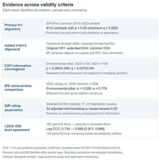
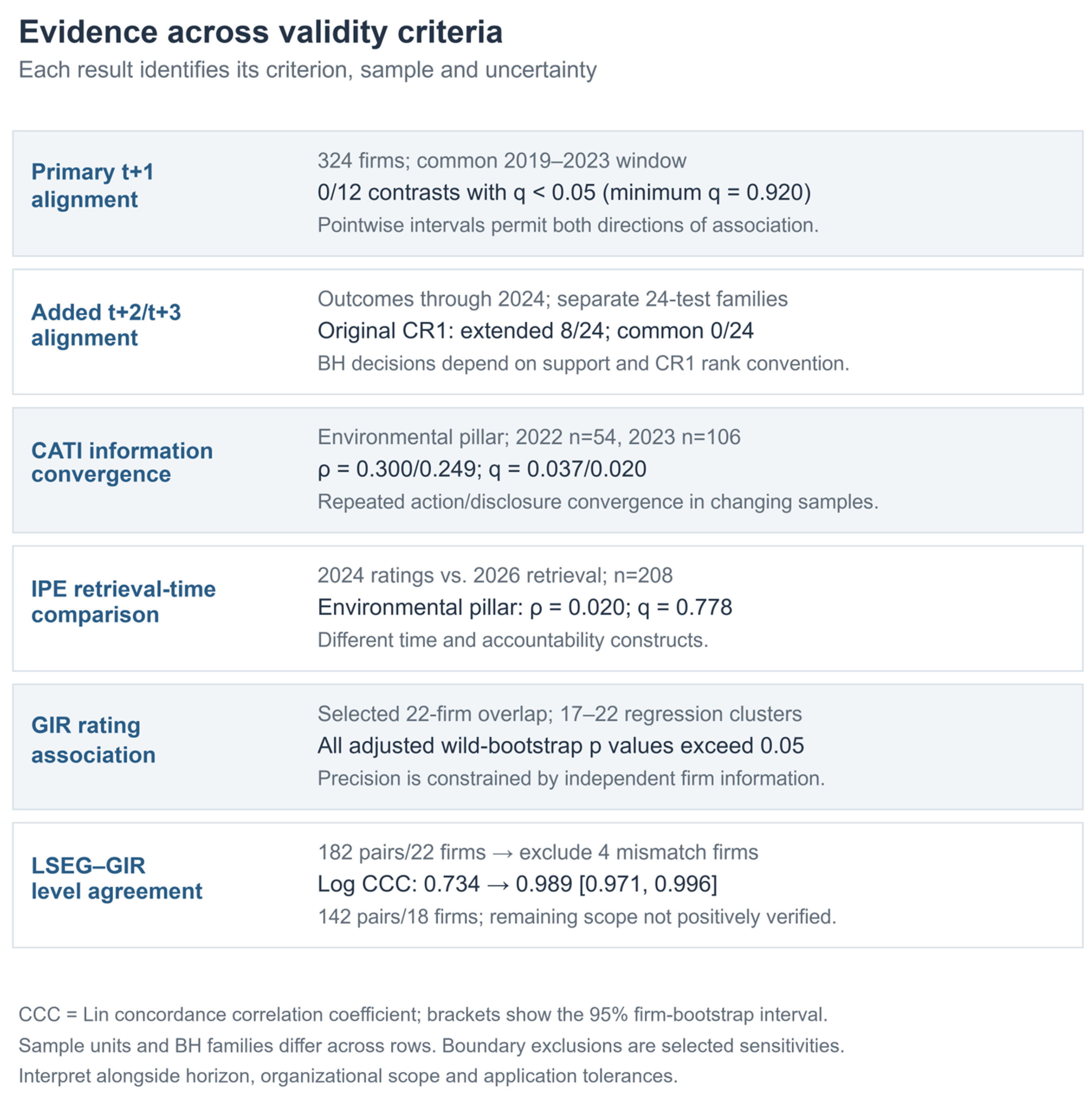
Figure 4 synthesizes the four criterion-specific tests without implying a causal or sequential chain among CATI, reported intensity, GIR, and IPE.

Figure 4. Criterion-specific external-validation evidence map. Note. Rows show criterion-specific comparisons with different samples, units and test families. Longer-horizon entries use available-support analyses with outcomes ending in 2024 and separate 24-test BH families. Their classifications also depend on the finite sample covariance convention (Table S22). CATI and IPE entries concern the environmental-pillar score. CCC denotes log-scale Lin concordance; intervals use 9999 whole-firm resamples. The four-firm exclusion is a documentary-informed sensitivity (Table S20).

The evidence separates four decisions. CATI supports repeated action/disclosure convergence in changing Chinese samples. The full-panel emissions association depends on horizon and temporal support, with no common-window BH rejection. The IPE retrieval-time test provides no adjusted association with its distinct accountability rank. GIR supplies a small-cluster regulatory test and shows that direct source agreement improves sharply when documented scope mismatches are removed. Figure 4 pairs each result with its actual criterion and coverage.

5. Discussion

5.1. Selective Validity Rather than a Binary Verdict

The central finding is that validation changes with the criterion and design conditions. Ratings align with selected action/disclosure assessments; longer-horizon emissions associations appear in the extended history; and provider–regulator agreement improves markedly after documentary boundary exclusions. A single conclusion that ratings either work or fail would conceal these differences. The common-window estimates instead provide an explicitly bounded, still-imprecise assessment of subsequent revenue intensity.

The methods identify three different quantities. Fixed-effects regressions estimate longitudinal conditional rating intensity slopes and their country contrast. Rank correlations identify convergence with the matched external criterion in its observed cross-section. Paired agreement statistics distinguish co-movement from similarity in emissions levels and ratios. Interpreting each result on its own statistical scale makes the layered assessment useful for deciding whether ratings support screening, emissions comparison or source substitution.

This pattern is consistent with competing disclosure mechanisms. Ratings may capture targets, frameworks, reporting systems, controversies, and assurance, all of which matter for governance. Physical transition also depends on capital replacement, energy substitution, output, acquisitions, and organizational boundaries. The Korea Electric Power Corporation negative control illustrates the last point: accurate field date alignment did not make a consolidated company boundary equivalent to the available external reporting boundary. Environmental pressure may itself prompt stronger reporting. Because managerial intent is unobserved, a mismatch between scores and emissions is not evidence of deliberate greenwashing.

5.2. Temporal Support Is Part of the Estimand

Temporal support is part of the estimand. Under the archived covariance convention, extended-history associations at two and three years survive adjustment, whereas common-coverage associations do not. Identical-baseline comparisons preserve this coverage pattern, but the common analysis then has only three exposure years, 2019–2021. Statistical classification additionally depends on the finite sample covariance convention: counting the full absorbed-effect rank moves the minimum added-horizon extended-window q to 0.055. The estimated slopes remain unchanged. This distinction makes the evidence useful for planning longer follow-up without treating it as a settled finding of delayed abatement.

Coverage selection also changes the firms represented. Retained firms are larger and more highly rated than partially observed firms in both countries, while their intensity differences vary by country (Table S9). The results describe sustained-coverage listed firms, not the listed-company population. The retrospective 2026 download can incorporate provider revisions and backfilling; observed reporting dates improve alignment but cannot recreate a verified historical point-in-time information set.

5.3. The Meaning of the China–Korea Comparison

A common provider, standardization and model make the two conditional country slopes directly comparable. The common-window data do not precisely establish a persistent slope difference; the extended-horizon differences remain sensitive to temporal support. The contribution is a transparent comparison under aligned conditions, not an estimate of which country has better environmental performance.

External validation complements this comparison without requiring identical institutions. CATI ranks, IPE accountability records and GIR metric tons answer different measurement questions. The markedly improved GIR agreement after documentary exclusions also illustrates why institutional reporting scope must be examined before comparing physical levels.

5.4. Relation to Prior Evidence

Prior studies evaluate different criteria and effect scales (Table S23). Cregan et al. [16] examine airlines, including physical-output intensities and horizons up to five years. Qian and Liu [14] study carbon emission efficiency, while Zhang and Lai [15] examine corporate environmental performance around rating coverage. Park et al. [17] study an emissions-trading intervention with another rating provider. These quantities are not directly interchangeable with log metric tons per USD per standardized within-country–industry–year score unit. The comparison explains how the findings can coexist and why their published coefficients are not used as post hoc equivalence margins.

The contribution also extends research on rating disagreement and score composition [1,4,11]. Consensus among ratings is an information-system property; validity against future intensity and agreement with regulatory records require additional evidence. The present design evaluates these distinct links within one provider history while retaining their different samples and uncertainty.

5.5. Implications, Limitations, and Next Tests

For investment screening, ratings can organize information about governance and disclosure alongside separately assessed emissions trajectories. For lending and transition-finance monitoring, the relevant outcome must state the reporting period, revenue denominator, estimated-versus-reported status and organizational scope. For regulatory or contractual substitution of one emissions source for another, scope verification and a use-specific tolerance are required: even after documentary exclusions, only 73.9% of pairs lie within 20%. Ex post target delivery and reporting provenance remain important complements [50,51,52].

Three evidence limits guide the next tests. First, sustained provider coverage and complete cases define a selected population in a retrospective history. Second, the GIR validation has only 17–22 clusters and some concentrated predictor information. Third, time-varying confounding, persistence and prior-outcome associations prevent causal attribution. Classical mean-zero error confined to a linear dependent variable and orthogonal to regressors increases uncertainty without necessarily attenuating the slope; error in ratings, changing scope or reporting errors related to ratings can bias associations. The two emissions sources do not identify error variances or a reliability ratio for the full panel. Common-boundary calibration data are needed for such corrections.

Future extensions should combine longer, consistently observed histories with dated investment and digital-adoption measures. The present data cannot assess five- to ten-year transition performance under comparable country support. A bilingual report database could add independently coded boundaries, target delivery and adverse-information coverage, but report length or keyword counts alone would not validate those constructs. A direct digital-channel test would require dated bilingual adoption coding validated independently, followed by rating-by-adoption interactions and temporally ordered emissions outcomes.

6. Conclusions

This study implements layered criterion-validity testing for 324 coverage-screened Chinese and Korean listed firms. In the common 2019–2023 exposure window, the twelve original next-year contrasts do not survive BH adjustment and remain too imprecise to establish equivalence. Two- and three-year slopes in the extended history identify a potential longer-horizon pattern, with statistical classification depending on temporal support and the finite sample covariance convention. CATI supplies repeated annual action/disclosure convergence; IPE and the restricted GIR association tests address distinct criteria with more limited evidence.

The regulatory comparison makes scope a central empirical result: excluding four documentary-supported mismatch firms raises the LSEG–GIR concordance from 0.734 to 0.989 and sharply narrows ratio limits. Public report anchors directly support selected recent years, not all retained or excluded historical boundaries. The resulting validation protocol links each interpretation to its criterion, temporal support, organizational scope and precision.

Environmental ratings are most informative when used with dated, scope-specific emissions evidence and explicit purposes. The present estimates support that combined approach for the observed sustained-coverage firms; they do not establish a causal effect of ratings or a general verdict on unobserved companies and longer transition horizons.

References

- Berg, F.; Kölbel, J.F.; Rigobon, R. Aggregate confusion: The divergence of ESG ratings. Rev. Financ. 2022, 26, 1315–1344. [Google Scholar] [CrossRef] [Scilit]
- Avramov, D.; Cheng, S.; Lioui, A.; Tarelli, A. Sustainable investing with ESG rating uncertainty. J. Financ. Econ. 2022, 145, 642–664. [Google Scholar] [CrossRef] [Scilit]
- Gibson Brandon, R.; Krueger, P.; Schmidt, P.S. ESG rating disagreement and stock returns. Financ. Anal. J. 2021, 77, 104–127. [Google Scholar] [CrossRef] [Scilit]
- Ferro, A.; Marazzina, D.; Stocco, D. Uncovering ESG ratings: The (im)balance of aspirational and performance features. Corp. Soc. Responsib. Environ. Manag. 2025, 32, 5895–5917. [Google Scholar] [CrossRef] [Scilit]
- Kohler, M.; Da Costa, P.; Cluzel, F.; Umbricht, L. A review of corporate climate ratings: Assessing divergence from scientific expectations. Renew. Sustain. Energy Rev. 2026, 226, 116352. [Google Scholar] [CrossRef] [Scilit]
- Clarkson, P.M.; Li, Y.; Richardson, G.D.; Vasvari, F.P. Revisiting the relation between environmental performance and environmental disclosure: An empirical analysis. Account. Organ. Soc. 2008, 33, 303–327. [Google Scholar] [CrossRef] [Scilit]
- Hummel, K.; Schlick, C. The relationship between sustainability performance and sustainability disclosure: Reconciling voluntary disclosure theory and legitimacy theory. J. Account. Public Policy 2016, 35, 455–476. [Google Scholar] [CrossRef] [Scilit]
- Marquis, C.; Toffel, M.W.; Zhou, Y. Scrutiny, norms, and selective disclosure: A global study of greenwashing. Organ. Sci. 2016, 27, 483–504. [Google Scholar] [CrossRef] [Scilit]
- Michelon, G.; Pilonato, S.; Ricceri, F. CSR reporting practices and the quality of disclosure: An empirical analysis. Crit. Perspect. Account. 2015, 33, 59–78. [Google Scholar] [CrossRef] [Scilit]
- Simnett, R.; Vanstraelen, A.; Chua, W.F. Assurance on sustainability reports: An international comparison. Account. Rev. 2009, 84, 937–967. [Google Scholar] [CrossRef] [Scilit]
- Arena, M.; Azzone, G.; Piantoni, G.; Tabarelli De Fatis, B.I.; Wang, M. ESG rating disagreement and sustainability reporting: The role of reporting standards and assurance practices. Corp. Soc. Responsib. Environ. Manag. 2025, 32, 5446–5468. [Google Scholar] [CrossRef] [Scilit]
- Doan, M.H.; Sassen, R. The relationship between environmental performance and environmental disclosure: A meta-analysis. J. Ind. Ecol. 2020, 24, 1140–1157. [Google Scholar] [CrossRef] [Scilit]
- Christensen, H.B.; Hail, L.; Leuz, C. Mandatory CSR and sustainability reporting: Economic analysis and literature review. Rev. Account. Stud. 2021, 26, 1176–1248. [Google Scholar] [CrossRef] [Scilit]
- Qian, Y.; Liu, Y. Improve carbon emission efficiency: What role does the ESG initiatives play? J. Environ. Manag. 2024, 367, 122016. [Google Scholar] [CrossRef] [Scilit] [PubMed]
- Zhang, H.; Lai, J. Greening through ESG: Do ESG ratings improve corporate environmental performance in China? Int. Rev. Econ. Financ. 2024, 96, 103726. [Google Scholar] [CrossRef] [Scilit]
- Cregan, C.; Kelly, J.A.; Clinch, J.P. Are environmental, social and governance (ESG) ratings reliable indicators of emissions outcomes? A case study of the airline industry. Corp. Soc. Responsib. Environ. Manag. 2024, 31, 909–928. [Google Scholar] [CrossRef] [Scilit]
- Park, H.; Khue, P.M.; Lee, J. The effects of carbon emissions trading on profitability and value: Evidence from Korean listed firms. J. Int. Financ. Manag. Account. 2024, 35, 760–799. [Google Scholar] [CrossRef] [Scilit]
- Aswani, J.; Raghunandan, A.; Rajgopal, S. Are carbon emissions associated with stock returns? Rev. Financ. 2024, 28, 75–106. [Google Scholar] [CrossRef] [Scilit]
- Cepêda, C.; Monteiro, A.P.; Aibar-Guzmán, B. Decoupling in sustainability reporting: A systematic literature review. Corp. Soc. Responsib. Environ. Manag. 2025, 32, 2988–3007. [Google Scholar] [CrossRef] [Scilit]
- Bajic, A.; Kiesel, R.; Hellmich, M. Handle with care: Challenges in company-level emissions data for assessing financial risks from climate change. J. Clim. Financ. 2023, 5, 100017. [Google Scholar] [CrossRef] [Scilit]
- Venter, E.R.; Krasodomska, J. Research on extended external reporting assurance: An update on recent developments. J. Int. Financ. Manag. Account. 2024, 35, 390–428. [Google Scholar] [CrossRef] [Scilit]
- Lin, W.; Wang, Y.; Zhang, Q.; Peron, M.; Lu, J. Emerging opportunities or paradoxes: Assessing the effect of digital technology adoption on corporate carbon performance. J. Environ. Manag. 2025, 391, 126399. [Google Scholar] [CrossRef] [Scilit] [PubMed]
- Arslan, H.M.; Chengang, Y.; Komal, B.; Chen, S. Nexus between environmental disclosures and top management team characteristics: A systematic review. Environ. Sci. Pollut. Res. 2023, 30, 9763–9781. [Google Scholar] [CrossRef] [Scilit] [PubMed]
- Arslan, H.M.; Mubeen, M.; Chen, S.; Naseer, K.; Yaseen, S. Audit Committee Characteristics and Sustainability Disclosures—A Meta-Analytical Perspective. Pak. J. Commer. Soc. Sci. 2024, 18, 1032–1064. [Google Scholar] [CrossRef] [Scilit]
- Hedegaard, M.; Bracio, A.M.; Kusnezowa, D.; Salvador, R. Environmental impact of ESG investments: Addressing the lack of cross-industry calibration in current ESG ratings. Corp. Soc. Responsib. Environ. Manag. 2026, 33, 3247–3262. [Google Scholar] [CrossRef] [Scilit]
- LSEG Data & Analytics. Legacy ESG Scores Methodology. Document Version 2.0, Effective July 2026; Archived 11 August 2026. 2026. Available online: https://thesource.lseg.com/thesource/getfile/index/457af0b5-8d12-4671-add5-5d125a06edce (accessed on 11 August 2026).
- Cameron, A.C.; Miller, D.L. A practitioner’s guide to cluster-robust inference. J. Hum. Resour. 2015, 50, 317–372. [Google Scholar] [CrossRef] [Scilit]
- Benjamini, Y.; Hochberg, Y. Controlling the false discovery rate: A practical and powerful approach to multiple testing. J. R. Stat. Soc. Ser. B (Methodol.) 1995, 57, 289–300. [Google Scholar] [CrossRef] [Scilit]
- Institute of Public & Environmental Affairs. Listed Company Climate Action CATI Index 2022 Evaluation Report. 2023. Available online: https://wwwen.ipe.org.cn/reports/report_21777.html (accessed on 9 August 2026).
- Institute of Public & Environmental Affairs. Listed Company Climate Action CATI Index 2023 Evaluation Report. 2024. Available online: https://wwwen.ipe.org.cn/reports/report_22094.html (accessed on 9 August 2026).
- Institute of Public & Environmental Affairs. Chinese Listed-Company Environmental Performance Ranking [Dynamic Database]. Available online: https://www.ipe.org.cn/GreenSecurities/GreenStocks.html (accessed on 9 August 2026).
- Greenhouse Gas Inventory and Research Center. Statement-Emissions Statistics [Data Set]. Available online: https://www.gir.go.kr/home/index.do?menuId=37 (accessed on 9 August 2026).
- Cameron, A.C.; Gelbach, J.B.; Miller, D.L. Bootstrap-based improvements for inference with clustered errors. Rev. Econ. Stat. 2008, 90, 414–427. [Google Scholar] [CrossRef] [Scilit]
- Roodman, D.; Nielsen, M.Ø.; MacKinnon, J.G.; Webb, M.D. Fast and wild: Bootstrap inference in Stata using boottest. Stata J. 2019, 19, 4–60. [Google Scholar] [CrossRef] [Scilit]
- Financial Supervisory Service. Open DART: Financial Statement Data Service. Available online: https://opendart.fss.or.kr/guide/main.do (accessed on 9 August 2026).
- World Bank. GDP Deflator (Base Year Varies by Country), Korea, Rep. (NY.GDP.DEFL.ZS). Available online: https://data.worldbank.org/indicator/NY.GDP.DEFL.ZS?locations=KR (accessed on 9 August 2026).
- Korean Air. 2024 Korean Air ESG Report. 2024. Available online: https://kind.krx.co.kr/external/2024/07/05/000251/20240705000314/2024%20%EB%8C%80%ED%95%9C%ED%95%AD%EA%B3%B5%20ESG%20%EB%B3%B4%EA%B3%A0%EC%84%9C.pdf (accessed on 11 August 2026).
- Samsung Electro-Mechanics. 2023–2024 Sustainability Report. 2024. Available online: https://kind.krx.co.kr/external/2024/06/28/000289/20240627000783/2023-2024%20%EC%82%BC%EC%84%B1%EC%A0%84%EA%B8%B0%20%EC%A7%80%EC%86%8D%EA%B0%80%EB%8A%A5%EA%B2%BD%EC%98%81%EB%B3%B4%EA%B3%A0%EC%84%9C.pdf (accessed on 12 August 2026).
- CJ CheilJedang. Sustainability Report 2024. 2024. Available online: https://www.cj.co.kr/cj_files/2024_sustainability_report_ko.pdf (accessed on 12 August 2026).
- CJ CheilJedang. Sustainability Report 2025. 2025. Available online: https://www.cj.co.kr/cj_files/2025_sustainability_report_ko.pdf (accessed on 12 August 2026).
- KEPCO. Sustainability Report 2023. 2023. Available online: https://www.kepco.co.kr/eng/sustainability/esg-report-center/sustainability-report/boardList.do (accessed on 12 August 2026).
- KEPCO. Environmental ESG Data Centre: Greenhouse Gas Emissions. Archived 12 August 2026. Available online: https://www.kepco.co.kr/eng/sustainability/esg-data-center/environment/data/conts.do (accessed on 12 August 2026).
- Lin, L.I. A concordance correlation coefficient to evaluate reproducibility. Biometrics 1989, 45, 255–268. [Google Scholar] [CrossRef] [Scilit]
- McGraw, K.O.; Wong, S.P. Forming inferences about some intraclass correlation coefficients. Psychol. Methods 1996, 1, 30–46. [Google Scholar] [CrossRef]
- Koo, T.K.; Li, M.Y. A guideline of selecting and reporting intraclass correlation coefficients for reliability research. J. Chiropr. Med. 2016, 15, 155–163. [Google Scholar] [CrossRef] [Scilit] [PubMed]
- Bland, J.M.; Altman, D.G. Statistical methods for assessing agreement between two methods of clinical measurement. Lancet 1986, 1, 307–310. [Google Scholar] [CrossRef] [Scilit]
- Bland, J.M.; Altman, D.G. Measuring agreement in method comparison studies. Stat. Methods Med. Res. 1999, 8, 135–160. [Google Scholar] [CrossRef] [Scilit] [PubMed]
- Bland, J.M.; Altman, D.G. Agreement between methods of measurement with multiple observations per individual. J. Biopharm. Stat. 2007, 17, 571–582. [Google Scholar] [CrossRef] [Scilit] [PubMed]
- Nickell, S. Biases in Dynamic Models with Fixed Effects. Econometrica 1981, 49, 1417–1426. [Google Scholar] [CrossRef] [Scilit]
- Jiang, X.; Kim, S.; Lu, S. Limited accountability and awareness of corporate emissions target outcomes. Nat. Clim. Change 2025, 15, 279–286. [Google Scholar] [CrossRef] [Scilit]
- Comello, S.; Reichelstein, J.; Reichelstein, S. Corporate carbon reporting: Improving transparency and accountability. One Earth 2023, 6, 803–810. [Google Scholar] [CrossRef] [Scilit]
- Swinkels, L.; Markwat, T. Corporate carbon emissions data for equity and bond portfolios. Manag. Financ. 2024, 50, 118–139. [Google Scholar] [CrossRef] [Scilit]
Disclaimer/Publisher’s Note: The statements, opinions and data contained in all publications are solely those of the individual author(s) and contributor(s) and not of MDPI and/or the editor(s). MDPI and/or the editor(s) disclaim responsibility for any injury to people or property resulting from any ideas, methods, instructions or products referred to in the content. |
© 2026 by the authors. Licensee MDPI, Basel, Switzerland. This article is an open access article distributed under the terms and conditions of the Creative Commons Attribution (CC BY) license.