


Abstract
Accurate ice-period river monitoring is essential for characterizing ice jam floods (IJFs) and associated jam-release waves (JAVEs). However, physics-based and machine-learning (ML) approaches remain constrained by data scarcity, uncertainty, and incomplete observations. This study develops a physics-verified data fusion and preprocessing workflow combined with Bayesian-optimized ML classification (PV-DFBML) for six IJF/JAVE states at Beauceville on the Chaudière River. The workflow utilizes a three-stage data refinement pipeline. First, categorical fusion of remote sensing (Sentinel-1/2, Landsat-8, and MODIS) and meteorological data isolates physically relevant ice regimes. This is followed by spatiotemporal validation and gap-filling of water level data to preserve longitudinal hydraulic consistency, alongside multi-step anomaly screening (DBSCAN and CUSUM) cross-checked against upstream–downstream consistency to isolate sensor noise. Among five Bayesian-optimized classifiers, B-RF achieved the strongest performance under the common 5-fold validation framework, with BACC = 0.76, MCC = 0.89, and minority-class F1 = 0.83. Full-winter input records provided the strongest classification skill, while physics-verified preprocessing improved minority-event detection. Random undersampling modestly increased BACC and minority F1 to 0.79 and 0.84, respectively, while reducing MCC to 0.85, indicating a trade-off in imbalance treatment. More stringent leave-one-winter-out validation yielded mean BACC = 0.68 ± 0.10, MCC = 0.61 ± 0.13, and minority F1 = 0.65 ± 0.09, demonstrating greater difficulty in generalizing to unseen winters. Transfer to Saint-Joseph-de-Beauce without site-specific retraining further reduced BACC to 0.67, MCC to 0.71, and minority-class F1-score to 0.67. Overall, the results demonstrate the importance of physically consistent data refinement while highlighting limitations associated with rare-event representation and temporal and spatial generalization.
1. Introduction
Rivers in cold regions are subject to both open-water floods and ice jam floods (IJFs). During mid-winter or spring breakup, increases in discharge (Q) and temperature can fracture the ice cover into discrete blocks, detach it from the riverbanks, and drift it downstream with the flow [1]. When downstream obstacles or a stable ice cover impede ice transport, backwater conditions may develop and generate hazardous IJFs. In dynamic river systems, these events may be followed by successive releases, producing ice jam release waves (JAVEs) that further increase flood risk for riparian communities [2,3,4]. Monitoring and characterizing these processes are therefore important for emergency preparedness, particularly in high-risk systems such as the Chaudière River, QC [5]. However, accurate prediction remains difficult because river ice processes are highly chaotic, and seasonal records commonly contain stochastic noise, discontinuities, and missing values.
Approaches for IJF prediction have evolved from empirical and regression-based methods toward machine learning (ML) and hydraulic modelling [4,6]. Recent studies have shown that ML models such as artificial neural networks (ANNs), support vector machines (SVMs), and extreme learning machines (ELMs) can capture nonlinear controls on mid-winter and spring breakup timing [4,7]. These studies have used hydrological, hydraulic, and meteorological time series as predictors, including air temperature, precipitation, solar radiation, ice thickness, Q, and water level (WL) [4].
Research at national, provincial, and reach scales has shown that several ML architectures can provide useful skill for ice-related prediction. For example, Random Forest (RF) models based on the Canadian River Ice Database (CRID) achieved 80% accuracy in classifying breakup severity and were applied to predict mid-winter breakup (MWB) occurrence across Canada [8]. In this study, correlation analysis, Least Absolute Shrinkage and Selection Operator (LASSO) regression, and input omission were used as pre-processing steps to improve prediction accuracy, and MWBs were classified into low, medium, or high severity categories [8]. In Québec, deep learning (DL) approaches, including combined Convolutional Neural Networks-Long Short-Term Memory (CNN-LSTM), reached F1 scores of 0.92 across 170 rivers for binary jam/no-jam classification [9]. Several alternative models, including SVM, k-Nearest Neighbors (kNN), Decision Tree (DT), Multilayer Perceptron (MLP), CNN, LSTM, and combined CNN-LSTM, were also evaluated [9]. At the reach scale, in the Saint-Joseph-de-Beauce sector of the Chaudière River, recent work has utilized ELM combined with k-fold cross-validation and normalization for IJF prediction [10,11]. Outside Canada, attempts to address data scarcity have included the integration of ERA5 meteorological reanalysis data with wavelet transform-genetic programming (WT-JBGP) for IJF prediction on the Tornio River [12]. The study used input data from the 10 days preceding IJF events and reported an overall accuracy (OACC) of approximately 0.91, a Heidke Skill Score exceeding 0.78, and a Positive Predictive Value above 0.85 [12].
Despite these advances, several methodological and data-related gaps remain. Much of the recent literature remains model-centered rather than data-centered [13,14,15]. In many cases, model performance is assessed using raw or only lightly processed datasets, without a systematic evaluation of the physical reliability of the input signals during ice-affected periods [8,10,11,12]. Although some studies have applied limited pre-processing, fewer have examined integrated workflows that combine regime isolation, gap filling, and multi-station hydraulic consistency checks within ML-based IJF prediction. Such preprocessing-based physical intervention differs from physics-informed or physics-constrained models in which governing equations, conservation laws, or process-based ice-dynamics relationships are embedded directly within the model architecture, loss function, or optimization procedure. In the present context, physical knowledge is used primarily to refine, verify, and structure the input data before ML training rather than to impose explicit physical constraints during model learning. In addition, previous work has focused mainly on algorithm selection under relatively static event definitions, typically considering binary (jam versus no-jam) or multi-severity classification targets without considering the temporal sequence of events [7,8,9,10,11,12]. A critical gap remains in integrating multi-sensor satellite fusion with Bayesian-optimized ML to predict the sudden release waves (JAVEs) that follow stable jams. The transition from IJFs to JAVEs has received less explicit attention within such modelling frameworks. Finally, the effect of input data length on prediction stability remains insufficiently examined, particularly under sparse and imbalanced seasonal records.
To address these gaps, this study develops a multi-stage physics-verified data fusion and pre-processing workflow with Bayesian-optimized machine learning (PV-DFBML) for the Town of Beauceville on the Chaudière River. The objective is to evaluate whether PV-DFBML can improve multiclass prediction of different IJF severity and JAVE states. The proposed approach includes: (1) a categorical fusion strategy that cross-references historical IJF records with multi-sensor satellite observations, including Sentinel-1 SAR, Sentinel-2, Landsat 8 imagery, and MODIS-derived albedo, to isolate ice-affected windows. This step is further supported by cross-station verification to maintain consistency with streamwise river ice conditions; (2) a multi-step physics-verified data fusion (PV-DF) pipeline designed to produce temporally consistent and hydrologically interpretable datasets for ice-affected seasons; and (3) application of ML classifiers (SVM, kNN, DT, ELM, RF) to classify individual IJF severity and JAVE states, followed by an event-scale temporal assessment of the chronological sequence of the predicted classes, extending beyond binary jam/no-jam classification. The study further evaluates the proposed workflow through a systematic sensitivity analysis. First, an assessment compares model performance using raw and refined PV-DF datasets to quantify the influence of physics-verified preprocessing on multiclass prediction capability. Second, a temporal sensitivity analysis investigates the effect of varying input durations, ranging from full-winter records to 10-day input windows, to identify the temporal scale that best supports multiclass prediction robustness and stability. Together, these analyses provide a structured evaluation of how data refinement and input-window selection influence machine learning performance for predicting IJFs and JAVEs. Accordingly, the technical boundary of the present study is that physical knowledge is incorporated at the data-fusion, quality-control, and preprocessing stages, while the ML classifiers themselves remain data-driven and do not explicitly solve or enforce river-ice governing equations.
2. Study Site and Data
2.1. Site Description
Figure 1 presents a location map for the Chaudière River watershed. The Chaudière River, originating from Mégantic Lake, flows northward for 192 km before joining the St. Lawrence River south of Quebec City, Canada (Figure 1). The watershed covers 6695 km2 and includes multiple tributaries with sub-watersheds ranging from 10 to 900 km2 [16]. The watershed spans diverse physiographic and hydrological settings, from the forested headwaters in the Upper Chaudière to the more urbanized downstream reaches, resulting in pronounced spatial variability in runoff generation, river hydraulics, and ice processes. The river is commonly divided into the Upper, Intermediate, and Lower Chaudière reaches. The present study focuses on the Intermediate reach, specifically the Beauceville sector, because it is a recurrent IJF zone. Despite construction of the Sartigan Dam in 1967, Beauceville has continued to experience IJFs since the late nineteenth century, including major recent events in 2014, 2016, 2017, 2019, and 2020 [17,18]. This history makes the reach an appropriate test site for evaluating IJF and JAVE prediction under recurring ice-affected conditions. Direct observations of ice thickness, water temperature, and icebreaker activity were not included because such information was not available as a continuous and spatially consistent record for the Beauceville reach during the study period. In addition, such information is often difficult to monitor continuously because of winter field access limitations, spatial heterogeneity of ice processes, and inconsistent operational reporting [4,17,19]. This data limitation further motivates the use of a data-centric framework based on variables that are routinely available, physically interpretable, and suitable for long-term reconstruction and verification.
Figure 1.
A location map showing the watershed area of the Chaudière River together with the weather and hydrometric stations and urban regions used in this study.
2.2. Hydrometeorological Data Sources
The proposed framework integrates meteorological, hydrometric, and derived hydroclimatic variables. Daily meteorological data, including air temperature and total precipitation, were obtained from the Beauceville weather station (7028754), operated by Environment and Climate Change Canada (ECCC) (Figure 1). WL at Beauceville was monitored by the Comité de Bassin de la Rivière Chaudière (COBARIC) network at 1-min resolution. Daily maximum WL was then retained for the analysis. Q was derived from the Sartigan (Station 023429) and Famine River (Station 023422) stations, operated by the Centre d’expertise hydrique du Québec (CEHQ). Daily Q at Beauceville was estimated by adding discharges from these upstream stations and scaling them by watershed area ratios, following the method described in [17].
The study also used cumulative degree days of thaw (CDDT) and accumulated degree days of freezing (ADDF) to represent antecedent thermal conditions during the ice season [5].
2.3. Ice Jam Flood Records, Verification, and Event Classification
IJF and JAVE occurrences were catalogued and verified using a multi-source data-fusion approach. Data fusion refers to the integration of hydrometric, meteorological, historical, and remote-sensing information for ice regime isolation, event verification, and dataset refinement. Event identification relied on high-resolution hydrometric time series, upstream and downstream WL observations, meteorological data, historical IJF records, field observations, and remote sensing products. Historical information and field observations were compiled from archives, media reports, interviews, satellite imagery, and CRID by [20]. These data were used in the current study to verify whether observed WL rises during breakup was associated with ice processes rather than open-water flooding.
To reduce false positives in JAVE identification, labels were further checked using a cross-platform remote-sensing strategy. MODIS-derived albedo was used for daily monitoring of river surface reflectivity and for detecting rapid albedo reductions consistent with ice clearance. Higher-resolution Sentinel-1, Sentinel-2, and Landsat-8 imagery were used to confirm ice presence, breakup, and open-water conditions. Throughout the study period, ice-season conditions and candidate IJF/JAVE events were also reviewed by members of the River Ice Laboratory using available field measurements and camera observations. These observations were cross-checked with upstream–downstream hydrometric responses and subsequently verified against MODIS, Sentinel-1/2, and Landsat-8 imagery. Therefore, satellite information was used as an additional independent verification layer rather than as the sole basis for event labeling. This combined approach supported the distinction between IJF-related WL rises, JAVE-related hydraulic release signals, and open-water spring flows. All verified events were organized into a six-class scheme as presented in Table 1.
Table 1.
Classification and grouping of ice phenomena.
According to Table 1, Class 0 represents no-flood conditions under ice cover; Classes 1 to 4 represent increasing levels of IJF severity defined from WL thresholds by the Système de Surveillance de la Rivière Chaudière (SSRC), operated by COBARIC since 2008 [11,16,20]. In contrast, Class 5 represents JAVE conditions and is treated separately because it reflects a distinct post-jam hydrodynamic response following the partial or complete release of an ice obstruction. This interpretation is supported by event chronology, rapid stage fluctuations, and historical and remote-sensing evidence of ice breakup and downstream wave propagation. Unlike Classes 1–4, which are defined by stage thresholds, Class 5 is process-based and was verified against upstream surges using wave peak celerity above 3 m/s to distinguish true events from sensor noise [21]. Operationally, Class 1 represents an active ice-jam condition within the Surveillance WL range without evidence of jam release, whereas Class 5 is assigned when a verified jam-release sequence occurs; consequently, the two classes may overlap in absolute WL magnitude but differ in event chronology and physical state. At Beauceville, this definition also includes short-lived rebuilding surges during ice motion, as island and bridge constriction can temporarily act as a hydraulic bottleneck. The classification procedure followed a hierarchical decision sequence. First, the physical state was identified using the verified ice and hydraulic evidence: observations were classified as an active ice-jam condition when an ice obstruction was physically supported by the available hydrometric, field, and remote-sensing evidence, whereas a jam-release wave (JAVE) was assigned only when a release sequence was independently verified from the event chronology, rapid water-level response, and supporting hydraulic or remote-sensing evidence. Second, for observations identified as active ice-jam conditions, the Beauceville water-level thresholds were applied to determine the severity category (Classes 1–4: Surveillance, Minor, Moderate, and Major). Thus, the water-level thresholds determine the severity of an active jam but do not define the physical state itself. Class 5 is reserved for a verified post-jam release-wave state and is therefore not assigned according to the active-jam water-level severity thresholds.
Satellite data from multiple sources were integrated to verify the physics-verified labels given to a specific flood event. MODIS albedo was used to track ice clearance at daily resolution, while Sentinel-2 optical imagery and Sentinel-1 Synthetic Aperture Radar (SAR) imagery were used to confirm the contrast between ice-affected and open-water states. Together, these products provided physical support for the assigned IJF and JAVE labels and helped separate ice-related events from open-water spring freshets. An example of such verification is shown in Figure 2. Figure 2A (3 April 2018) from Sentinel-2 shows the river during a period categorized as a Class 1 surveillance flood. The bright, cyan-to-white spectral signature within the river channel indicates the physical presence of an ice jam and deteriorating ice cover. During this event, WLs were recorded between 149.6 m and 150.8 m.
Figure 2.
Remote-sensing verification of ice and open-water conditions: (A) Sentinel-2 image showing Class 1 surveillance-flood conditions on 3 April 2018; (B) Sentinel-2 image showing open-water conditions on 23 April 2018; (C) Sentinel-1 image (IW mode, VV/VH polarization, gamma0 backscatter in dB) showing IJF conditions on 4 April 2020; and (D) Sentinel-1 image showing open-water conditions on 16 April 2020.
This visual evidence confirms that the WL rise was driven by ice-related resistance rather than purely hydrodynamic flow, justifying its classification within the breakup and ice deterioration phase. In contrast, Figure 2B (23 April 2018) shows the same reach 20 days later. The river channel appears as a dark, continuous linear feature, signifying open-water conditions following the mechanical breakup and downstream passage of ice. To bridge the data gaps caused by cloud cover in Sentinel-2 imagery, Sentinel-1 SAR imagery (Figure 2C,D) was used. The high backscatter in Figure 2C reflects the surface roughness of chaotic ice rubble, physically justifying the IJF label on 4 April 2020. Conversely, the low backscatter in Figure 2D signifies specular reflection from smooth open water on 16 April 2020. This dual-sensor approach ensures that peak WL values are strictly associated with the physical presence and release of ice jams rather than open-water spring freshets.
3. Methodology
3.1. Methodology Overview
In this study, a PV-DFBML is developed as an integrated workflow rather than a single black-box predictive classifier. Figure 3 presents a schematic overview of the methodology used to develop the PV-DFBML framework. The framework combines physics-verified data fusion and quality control (PV-DF) with Bayesian optimization of ML classifiers. Thus, the term physics-verified refers to the pre-processing, event verification, and data-selection stages, whereas the ML component remains data-driven. The purpose of the framework is to evaluate how physically guided refinement of hydroclimatic records influences the skill of multiclass IJF/JAVE state prediction. The ML classifiers operate pointwise and assign an IJF/JAVE class to each individual observation; they do not explicitly model state-transition probabilities or sequential dependence. Temporal progression is evaluated subsequently at the event scale by arranging the independently predicted classes chronologically and comparing their sequence with the observed evolution of each breakup event. Accordingly, the framework prioritizes the physical integrity and spatiotemporal continuity of hydrometeorological inputs before model training. It operates through three sequential phases: (1) an integrated data-centric pre-processing pipeline, (2) physics-verified quality assurance and verification, and (3) Bayesian-optimized model development and sensitivity analysis.
Figure 3.
Flowchart of the research methodology.
The framework begins by aggregating the main hydrometeorological variables used in the study, including WL, Q, air temperature, CDDT, ADDF, and precipitation (Figure 3). Ice-affected periods are identified using MODIS-derived albedo together with higher-resolution Sentinel-1/2 and Landsat-8 imagery in order to define the temporal analysis window. After isolating the ice-presence period, the continuity of the time series is evaluated. Missing values are then reconstructed using spatially and temporally informed approaches, including Inverse Distance Weighting (IDW), Multivariate Linear Regression (MLR), and substitution from nearby stations, depending on data availability and gap characteristics. These reconstructions are based on covariates selected to preserve local watershed behavior [18,22].
Following gap filling, anomalous observations are screened using the Interquartile Range (IQR) and Density-Based Spatial Clustering of Applications with Noise (DBSCAN) methods [23,24]. Flagged values were subsequently checked through spatiotemporal verification by testing whether a WL spike at Beauceville was reflected at Saint-Georges or Saint-Marie within a physically realistic lag, and whether the anomaly was consistent with discharge evolution and known ice-event timing. Where available, Sentinel and MODIS observations were also used to confirm ice presence, breakup, or open-water conditions. Values that were not supported by this combined hydraulic and observational evidence were classified as sensor-related anomalies rather than plausible hydrological extremes. After this stage, time-series stability is examined using change-point detection and homogeneity tests, including the Cumulative Sum (CUSUM), Standard Normal Homogeneity Test (SNHT), and Buishand U-test [24,25]. Because these preprocessing operations are applied sequentially, the output and interpretation of one stage can influence subsequent stages. Therefore, the PV-DF pipeline was evaluated primarily as an integrated data-refinement workflow; the raw-versus-refined comparison quantifies its overall effect on prediction performance rather than attributing performance changes to individual preprocessing components.
The refined datasets were then used to train different models capable of classifying IJF/JAVE states. Finally, model outputs were validated using independent observations, satellite imagery (e.g., MODIS), and event-based records from the historical IJF dataset to identify the most suitable ML model for multiclass IJF/JAVE prediction.
3.2. Multi-Step Data Pre-Processing
3.2.1. Missing Value Imputation Strategies
Missing values were identified considering the hydraulic connectivity within the river network. Depending on gap duration and variable type, MLR, IDW, or substitution from nearby correlated stations was used to preserve spatial and temporal hydraulic consistency. Table 2 summarizes the gaps in each time series and the methods used for infilling.
Table 2.
The number of gaps in each time series and methods used to fill these gaps.
This classification guided the selection of the most appropriate infilling method. For air temperature and total precipitation, the nearby Saint-Georges station (7027283), located within 15 km of the target Beauceville stations (7020560 and 7028754), was used for direct substitution because of its strong correlation with the target records (R > 0.95). Where similar gaps occurred and no suitable station data were available, values were directly replaced using NCEP/NCAR Reanalysis data [26].
For WL, short gaps were filled using IDW from upstream (Saint-Georges, StG) and downstream (Saint-Marie, StM) stations (Figure 1) [11]. Medium and long gaps or cases in which IDW was insufficient were filled using an MLR model based on Q and WL from the nearby StG and StM stations. This model used hydrologically connected predictors that were strongly correlated with WL at Beauceville, as indicated by Pearson correlation coefficients between Beauceville WL and QStG (0.862), QB (0.865), and WLStM (0.841). To preserve calibration integrity, the MLR model was trained only on complete annual records. The preprocessing stage was implemented as a retrospective reconstruction and quality-control procedure for the historical record prior to ML model development. Annual records were used for gap-filling model development, while reconstructed and statistically flagged observations were subsequently evaluated using hydrological and cross-station consistency checks. Different data transformations (raw, logarithmic, z-score, robust scaling) and model forms (linear and second-degree polynomial) were tested, and performance was evaluated using the coefficient of determination (R2), adjusted R2, p-values, Mean Squared Error (MSE), Root Mean Squared Error (RMSE), Mean Absolute Error (MAE), and residual error metrics. Estimated values were then checked against upstream and downstream stations and historical IJF records. It should be emphasized that the downstream Saint-Marie WL was used only as an external spatial covariate for retrospective reconstruction and hydraulic-consistency verification of missing Beauceville observations. Saint-Marie WL was not included as a predictor in the final IJF/JAVE classification model, and no recursive feedback between the two stations was introduced. Thus, its use represents spatial reconstruction of an incomplete historical record rather than a causal upstream forecasting relationship. For real-time implementation, the reconstruction procedure would need to be restricted to observations available at or before the prediction time.
For Q, missing values were estimated using upstream measurements from Saint-Martin (023448) on the Chaudière River and Du Loup (023428) on the Du Loup River using the drainage-area ratio approach described in [17]. In that study, watershed-area ratios were used to distribute lateral tributary contributions along the river during calibration of an ice-cover HEC-RAS model. Specifically, discharge at a downstream confluence was related to the reference discharge at Sartigan Dam according to the ratio of their contributing watershed areas. The authors selected this approach instead of a uniformly distributed lateral inflow so that the spatially non-uniform contributions of tributaries could be represented when the hydraulic model simulated ice-cover and ice-jam backwater conditions. In the present study, the same drainage-area concept was adopted because it was developed and applied for the same Chaudière River system.
3.2.2. Outlier Detection and Correction
To isolate sensor anomalies from physical hydrologic extremes, a dual-layer filter was employed. DBSCAN was utilized for multivariate anomaly detection, while the IQR method targeted univariate spikes. Values flagged as potential outliers were then checked against upstream (StG) and downstream (StM) stations to ensure that true rapid-onset flood signals were not removed.
DBSCAN is a density-based clustering algorithm that identifies clusters of densely packed points and treats low-density points as outliers. For each point (p), the algorithm examines its ε-neighborhood as shown in Equation (1) [27].
where N ε (p) is the set of points within the ε-neighborhood of p. q represents any arbitrary point within the dataset D. D is the total dataset being analyzed. d(p,q) is the distance metric (e.g., Euclidean distance) between points p and q. ε is the radius defining the neighborhood around each point. If the number of neighboring points within this radius (defined as the distance threshold ε) meets or exceeds the threshold of minimum number of points (MinPts), the point is labeled as a density-representative point (core point). Points that are not density-reachable from any core point are classified as anomalies. DBSCAN is particularly useful for detecting outliers in data with non-linear structures [27].
N ε (p) = {q ∈ D∣ d(p,q) ≤ ε}
The IQR method, based on Tukey’s boxplot approach [28], identifies outliers by calculating the interquartile range IQR = q3 − q1 and determining fences (Equation (2)) beyond which values are considered potential outliers.
where q1 and q3 represent the first and third quartiles, respectively, and IQR is defined as q3 − q1. The standard boxplot is particularly suited for normal or symmetric distributions. For Gaussian data, the probability of an observation falling below (q1 − 1.5 × IQR) or above (q3 + 1.5 × IQR) is approximately 0.35% (0.0035 probability) in each tail [18,29].
Fence = (q1 − 1.5 × IQR, q3 + 1.5 × IQR)
The data refinement is termed physics-verified (PV) because anomaly screening follows strict hydraulic consistency rules. Potential anomalies identified by DBSCAN and IQR-based screening were not removed automatically; instead, flagged observations underwent a second-stage physical verification based on temporal continuity, hydraulic consistency with neighboring stations, and consistency with known ice-event timing. For example, a sudden stage rise at Beauceville was preserved only if it was accompanied by a corresponding discharge surge at other stations within a physically plausible wave-travel time, or if satellite imagery confirmed downstream ice accumulation. In practice, this verification assessed whether a WL spike at Beauceville was also reflected at Saint-Georges or Saint-Marie within a realistic time lag (see Figure 1). Values not supported by this cross-station behavior were interpreted as sensor-related anomalies and corrected through the PV-DF pipeline. The practical motivation for this verification procedure is to ensure that the prediction framework receives reliable hydrometric observations from an operational monitoring network. Although WL is recorded directly at the target site, temporary sensor malfunction, missing observations, drift, or isolated measurement errors may occur and therefore require verification before the data are supplied to the ML framework. This issue is particularly important during ice-affected conditions because ice-induced resistance and backwater can alter the conventional open-water relationship between discharge and stage [1]. Consequently, an abrupt or statistically anomalous WL value cannot be considered erroneous solely because it deviates from the expected open-water hydraulic response. This quality-control step is intended to preserve physically meaningful IJF and JAVE signals while correcting only observations supported as measurement-related anomalies. For prospective application of the framework, such verification should rely exclusively on observations available at or before the prediction time.
3.2.3. Change-Point Analysis and Homogeneity Testing
To assess long-term consistency of the time series, homogeneity and change-point analyses were conducted using SNHT and the Buishand U test for homogeneity assessment, and the CUSUM test for change-point detection. These methods are commonly applied in climatology and hydrology to identify abrupt or gradual shifts in the mean associated with measurement changes, instrumentation effects, or hydrological regime changes [8,30]. In this study, the tests were used to help distinguish sensor drift from genuine hydrological variability.
The CUSUM test detects shifts in the mean by computing cumulative sums of deviations from the overall mean and is computed as Equation (3).
where xi represents the observed values, µ is the mean of the time series, and Sk is the cumulative sum up to time k. The absolute maximum value of Sk is used as the test statistic that highlights both sudden and gradual changes and is effective for long-term hydrological records [30]. The test was applied recursively to each time series. A threshold value of 15 and a minimum segment length of 700 were used to avoid over-segmentation. Change points were identified at the location of maximum cumulative deviation, and segments with significant changes were split and retested recursively.
SNHT compares the means of two data segments across all possible split points using a normalized test statistic Tk. It is particularly sensitive to both small and large shifts in the mean and is widely applied for homogeneity analysis in climatological time series [31]. The SNHT test statistic Tk at each point k is defined as Equation (4).
where µ1 and µ2 are the means of the first and second segments of the time series, respectively, µ is the overall mean, and σ2 is the variance of the time series. The maximum value of Tk is used as the test statistic to identify the most likely change point. Large values of Tk indicate a significant shift in the mean, suggesting a potential structural break in the data.
Finally, the Buishand U test is another non-parametric method designed to detect abrupt shifts in the mean Uk (Equation (5)).
where µ is the mean of the entire time series, and xi represents the observed values. The most likely change point (K) is identified by maximizing the absolute value of Uk [32].
For both SNHT and Buishand tests, recursive binary segmentation was applied. When the U or T statistic exceeded the critical threshold, the series was split at the detected point and each subsegment was re-tested. Segments were then labelled as homogeneous or inhomogeneous [31]. Values identified as suspicious by these tests were cross-validated against nearby stations to assess spatial hydraulic consistency with historical trends and hydrological behavior. Values that failed this multi-station verification were replaced using the corresponding gap-filling procedures.
3.3. Feature Selection and Normalization
After producing the reliable datasets, feature selection was performed to identify the most informative predictors for modelling. Mutual Information (MI) was employed, as it has been shown to outperform alternative methods in similar contexts [11]. Based on MI ranking, one day lag of WL, Q, total precipitation, mean temperature, CDDT, and ADDF were selected as the inputs for model development, consistent with previous studies where similar predictors were identified as important for IJF modelling [8,11,33]. Mutual Information ranking was performed using the training subset within each cross-validation iteration, and the selected predictors were then applied to the corresponding validation subset. The target is formulated as a multiclass river-ice state classification using antecedent hydrometeorological information. For each target day (t), one-day-lagged WL, Q, total precipitation, mean air temperature, CDDT, and ADDF from the preceding day (t − 1) are provided as model inputs to classify the IJF/JAVE state associated with day (t). Thus, the one-day lag represents antecedent conditions used for state classification; it should not be interpreted as an operational one-day-ahead forecast because the present study does not evaluate forecasts issued at a defined forecast origin for a future (t + h) target. Accordingly, the present analysis is referred to as lagged-input multiclass classification. The term prediction is used in the general machine-learning sense of an estimated class label, whereas prospective forecasting is reserved for future implementations with an explicitly defined lead time.
Following feature selection, z-score normalization was performed within each cross-validation iteration, with normalization parameters estimated from the training subset and subsequently applied to the corresponding validation subset. Model evaluation was conducted using 5-fold cross-validation as an internal comparative framework for model development and sensitivity analysis [11]. This approach provided a consistent basis for comparing candidate classifiers and antecedent input windows under identical dataset and preprocessing conditions. Because the folds were not structured as chronologically independent ice seasons, these metrics were not interpreted as strict estimates of out-of-time temporal generalization.
3.4. Bayesian-Optimized Machine Learning Models
In this study, five ML classifiers commonly used in IJF studies were employed and optimized using Bayesian optimization to predict the multiclass IJF/JAVE state during the ice-affected period [4]. These models were Bayesian-optimized-DT (B-DT), Bayesian-optimized-kNN (B-kNN), Bayesian-optimized-SVM (B-SVM), Bayesian-optimized-ELM (B-ELM), and Bayesian-optimized-RF (B-RF). The selected models represent different learning paradigms, including rule-based decision tree learning (B-DT), ensemble learning (B-RF), instance-based distance learning (B-kNN), margin-based kernel learning (B-SVM), and randomized neural network learning (B-ELM). This range of model structures was used to compare how different ML approaches capture nonlinear relationships and class separation in ice-affected hydrological datasets [8,33,34]. Each model was developed as a classifier capable of distinguishing multiple severity classes.
For each classifier, hyperparameters were tuned using Bayesian optimization over the ranges summarized in Table S1. Rather than using exhaustive search, this approach uses a probabilistic surrogate model to explore the hyperparameter space efficiently by balancing exploration and exploitation. The selected classifiers were intended to represent different conventional ML learning paradigms rather than to provide an exhaustive benchmark of all available classifier architectures. Therefore, the term best-performing model in this study refers specifically to the models evaluated herein and does not imply global optimality relative to untested models. To evaluate the specific contribution of Bayesian hyperparameter optimization, the selected B-RF configuration was additionally compared with a standard RF using the default hyperparameters under the same 5-fold cross-validation framework.
3.5. Class-Imbalance Sensitivity Analysis
To evaluate the sensitivity of the selected Bayesian-optimized Random Forest (B-RF) to strong class imbalance, Random undersampling (RUS) was evaluated as a sensitivity analysis. SMOTE was also considered as a potential oversampling alternative but was not implemented because the rarest major IJF class contained only two observations. RUS reduces the dominance of the majority class by randomly removing a proportion of its observations while retaining the available minority-class samples, thereby producing a more balanced training distribution [35]. Conventional SMOTE relies on interpolation among neighboring minority observations, and its effectiveness can be limited under severe small-sample class imbalance [36]. Given that only two major IJF observations were available, synthetic oversampling could disproportionately reproduce the characteristics of individual extreme events rather than represent the underlying variability of this class. Therefore, the sensitivity analysis was restricted to RUS, which reduces majority-class dominance without generating artificial IJF/JAVE observations.
For the sensitivity analysis, the original B-RF model trained on the naturally imbalanced dataset was used as the reference configuration and compared with RUS-B-RF. To ensure that the effect of class-imbalance treatment was evaluated independently of model configuration, the same selected predictor variables, Bayesian-optimized RF hyperparameters, and cross-validation framework were maintained for both configurations. RUS was applied only to the training portion of each cross-validation fold, while the corresponding validation data retained their original class distribution to avoid information leakage and preserve realistic evaluation conditions.
3.6. Model Evaluation Metrics
Model performance was first evaluated using six widely accepted metrics derived from the confusion matrix. These included Accuracy, Precision, Recall, Specificity, F1- Score, and False Positive Rate (FPR), which provide a basic assessment of the models’ ability to correctly identify both IJF and non-IJF events and help evaluate classifier reliability and sensitivity to true events [11]. In addition, OACC, Balanced Accuracy (BACC), Cohen’s Kappa (κ), and Matthews Correlation Coefficient (MCC) were calculated to account for class imbalance and multiclass classification. Moreover, Precision, Recall, Specificity, F1-Score, and FPR were calculated using two distinct strategies: macro-averaging, which represents the simple arithmetic mean across all classes to provide an unweighted assessment, and weighted-averaging, which computes the mean by accounting for the relative support of each class. To specifically assess performance on IJF events, additional weighted metrics were computed while excluding the majority class. The corresponding equations are provided in Equations (6)–(14). For the purpose of this study, classes representing standard river conditions (i.e., non-event states) are defined as the majority class due to their dominance in the temporal record. In contrast, classes representing IJF and JAVE events are designated as minority classes because of their stochastic, infrequent nature. Because the dataset was imbalanced, Balanced Accuracy (BACC), Matthews Correlation Coefficient (MCC), macro-averaged metrics, and minority-class Precision, Recall, and F1-score were prioritized as the primary indicators of classification performance. These metrics provide a more representative assessment of performance across both dominant and infrequent IJF and JAVE classes. Overall Accuracy (OACC) was reported as a supplementary metric but was not used as the primary basis for model selection because it can remain high in strongly imbalanced datasets even when performance on minority classes is poor.
where True Positive (TP) is the correct detection of an event; True Negative (TN) is the correct identification of non-IJF; False Positive (FP) is incorrect IJF or JAVE prediction; and False Negative (FN) is missed actual IJF event, C is confusion matrix, s is total number of samples, pk is number predicted as class k, tk is number truly belonging to class k, po is observed agreement, and pe expected agreement by chance.
4. Results
The results are presented in three stages. First, the data-preprocessing outcomes are presented. Second, the predictive performance of the ML models are compared to identify the most suitable configuration for PV-DFBML. Finally, the selected model is evaluated for IJF and JAVE events.
4.1. Data Pre-Processing
4.1.1. Gap-Filling
Several MLR models were used to reconstruct missing WL values at Beauceville. These models were calibrated and validated using full years of complete data, and their performance is summarized in Table 3.
Table 3.
Comparative performance of different MLR models for WL gap-filling.
The raw-data MLR model yielded an R2 of 0.65, indicating only moderate explanatory power. Among the predictors, WLStM had the largest coefficient (0.889, p < 0.001), while QStG and QB also contributed positively but with smaller magnitude. However, the model retained relatively large errors (MSE = 0.27, RMSE = 0.52, MAE = 0.54), indicating limited accuracy under raw data. Applying the same MLR structure to transformed datasets improved performance. Among the tested options, the log-transformed MLR performed best, with an R2 of 0.77 and markedly lower errors (MSE = 0.01, RMSE = 0.11, MAE = 0.22). All predictors remained statistically significant (p < 0.001), and WLStM retained the strongest positive influence, followed by QStG, while QB showed a negative coefficient. Because the physical WL response may exhibit non-linear behavior, particularly during transitions between open-water and ice-affected conditions [1], a second-degree polynomial regression was also tested on the log-transformed dataset. This model improved on the raw-data MLR (R2 of 0.73, MSE = 0.03, RMSE = 0.17, MAE = 0.43), and all quadratic terms were statistically significant, particularly WLStM. However, its performance remained slightly below that of the simpler log-transformed MLR model.
Overall, the log-transformed MLR provided the strongest gap-filling performance for water level at Beauceville. The results suggest that transformation was more important than increasing model complexity for this task. On that basis, the subsequent data-refinement procedure retained a hybrid approach. The log-transformed MLR model was used as the primary reconstruction method because it showed the strongest overall quantitative performance, whereas IDW was applied selectively to short local gaps [11], where preservation of continuity with neighboring observations was prioritized.
4.1.2. Outlier Detection
This section compares the performance of the applied outlier detection methods for four key input variables including QStG, mean temperature at Beauceville (Mean TB), total precipitation at Beauceville (PreB), and WL at Beauceville (WLB). Following gap filling, outlier detection was performed using DBSCAN and IQR as shown in Table 4. The distinction between measurement error and physically meaningful events was then evaluated using Temporal-Spatial Verification and Correction (TSVC).
Table 4.
Comparative performance of outlier, change point, and homogeneity detection methods.
The IQR method consistently flagged the highest number of outliers, whereas DBSCAN detected substantially fewer points, reflecting the different mathematical assumptions underlying each method [37]. This contrast was most evident for QStG, where DBSCAN identified only four outliers whereas IQR flagged 155. Cross-validation against upstream stations (Du Loup and Saint-Martin) and precipitation records indicated that the DBSCAN-flagged events corresponded to physically plausible hydrological responses, including QStG = 778.6 m3/s following 101.2 mm of precipitation on 1 November 2019 and QStG = 611.7 m3/s during a December 2018 event with 52.1 mm of precipitation. In this case, the larger IQR count mainly reflected statistical sensitivity rather than confirmed error. Both methods were less reliable for mean temperature, likely because of strong regional thermal variability. Spatial comparison with StG confirmed only one true outlier for Tmean. For precipitation, IQR again returned a much larger count (201) than DBSCAN (10), which is consistent with the skewed and multimodal nature of precipitation distributions [38].
For WLB, flagged values were further evaluated through TSVC using upstream (StG) and downstream (StM) gauges. Most flagged points were associated with verified IJFs, JAVEs, or extreme precipitation rather than sensor error. For example, a 2019 WL fluctuation initially appeared anomalous after an IJF and three consecutive precipitation events with totals of 5.2 mm, 23.2 mm, and 35.8 mm, but cross-station comparison showed that the fluctuation remained within hydrodynamic bounds. Of the 73 IQR-flagged WL values, only 2 were validated as sensor errors, and 66% coincided with verified JAVEs or extreme events. These results indicate that purely statistical screening would have removed many event-related signals.
Overall, DBSCAN provided a more selective set of candidate outliers than IQR, whereas TSVC was necessary to determine whether flagged values represented measurement error or hydrologically meaningful extremes. The result is important because many large deviations during ice-affected periods corresponded to actual flood-related processes rather than noise.
4.1.3. Change-Point and Homogeneity
Temporal consistency was further assessed using CUSUM, SNHT, and the Buishand U test (Table 4). These methods identified periods of potential non-stationarity or inhomogeneity, which were then evaluated through TSVC to distinguish sensor-related anomalies from hydrologically consistent variability.
For QStG, CUSUM identified several non-stationary periods. The interval from November 2017 to April 2019 accounted for 58% of the detected change points, and additional clusters occurred during winters 2015–2018 and 2020–2023. These periods coincided with observed mid-winter breakups and variable winter flow conditions. After TSVC, all 21 suspicious QStG points were retained as physically plausible.
For Tmean, CUSUM detected statistical shifts during 2015–2016, 2016–2017, and the early 2020s. The detected changes were subsequently evaluated through the TSVC procedure using broader hydrometeorological and spatial records to distinguish measurement-related anomalies from physically consistent variability. Where the cross-dataset evidence indicated sensor-related inconsistencies, the corresponding observations were corrected; changes supported by the surrounding hydrometeorological records were retained as physically plausible variations. Because CUSUM accumulates deviations from the mean, it is more sensitive to sustained regime shifts than to isolated abrupt events [32]. For example, CUSUM identified a statistical shift around 1 March 2018 and additional changes after January 2020. The latter period contained approximately 50% fewer detected change points than the preceding period, indicating a difference in the statistical behavior of the time series. Although these changes coincided with variations in the broader hydroclimatic and river-ice records, neither CUSUM nor the subsequent consistency verification establishes their physical cause. Therefore, possible influences such as hydroclimatic variability, altered freeze–thaw conditions, or longer-term climatic changes are not attributed directly from the present analysis and would require a dedicated trend and attribution study.
For total precipitation, CUSUM identified changes in early 2019 (10 March 2019, 24 January 2019) and early 2023 (17 February 2023). Spatial validation within the TSVC confirmed two of these points as suspicious because they differed from the regional pattern by more than 15 mm.
WL displayed the clearest evidence of sensor-related instability. CUSUM detected abrupt shifts on 1 November 2019 and 2 November 2019, but these were reconciled with precipitation-induced surges of 28.1 mm and were supported by the downstream station (StJ). Of the 27 WL change points identified by CUSUM, only 3 were ultimately confirmed as true anomalies after TSVC; these values were removed and replaced using the selected gap-filling approach.
The homogeneity tests produced a similar contrast. The Buishand U test flagged more dates than SNHT, whereas SNHT was more selective. For QStG, temperature, and precipitation, TSVC supported overall homogeneity. In contrast, WL showed substantial inhomogeneity (i.e., artificial shifts and breaks) associated with sensor-related problems. In total, TSVC confirmed 45 WL values as erroneous and flagged them in both homogeneity tests. SNHT identified 16 dates, whereas the Buishand U test identified 45 of 72 suspicious points. These values were replaced using the gap-filling method.
In summary, the homogeneity and change-point analyses indicate that not all statistically detected shifts reflected measurement problems. In several cases, abrupt or gradual changes corresponded to real hydrological variability during ice-affected periods. For WL in particular, combining formal tests with TSVC and cross-validating the results with observed events reduced unnecessary correction while still identifying genuinely erroneous values.
4.2. Performance Evaluation of Bayesian-Optimized Machine Learning Models
Using the refined dataset, five Bayesian-optimized ML models were evaluated for IJF and JAVE prediction. The final hyperparameter values selected by Bayesian optimization for each classifier are reported in Table S1 of the Supplementary Materials together with the corresponding search ranges. The non-event states constitute the majority class, while the IJF and JAVE events are treated as minority classes. Because the dataset was imbalanced, BACC and MCC were selected as the primary indicators of overall classification performance, whereas Precision, Recall, and F1-score were used to evaluate minority class detection as presented in Figure 4. OACC was not considered sufficient on its own, as it can remain high in strongly imbalanced datasets even when performance on minority classes is poor.
Figure 4.
Performance of the models across different metrics.
According to Figure 4, B-RF achieved the strongest global classification performance, with an MCC of 0.89 and a BACC of 0.76, followed by B-ELM. In contrast, B-SVM showed the weakest overall performance, recording the lowest BACC (0.35) and MCC (0.45), which suggests limited capacity to distinguish among classes in this imbalanced hydrological dataset and to represent the overall pattern of IJF and JAVE occurrences. B-DT and B-kNN yielded moderate performance, with MCC values of 0.73 and 0.69, respectively.
The differences among models were most evident in their handling of minority classes as shown in Figure 4. B-RF achieved an F1-score of 0.83, indicating a superior ability to balance classification accuracy across both majority and minority classes. Furthermore, B-RF achieved the highest Precision (0.84), demonstrating a high degree of reliability in its flood warnings with the fewest false alarms. In comparison, B-DT and B-kNN yielded lower Recall values (0.57 and 0.50, respectively), suggesting reduced sensitivity to actual IJF and JAVE events.
For model comparison, both weighted and macro-averaged metrics were assessed. The weighted metrics remained substantially higher than the macro-averaged values, consistent with the expected influence of class imbalance. This gap indicates that predictive performance was stronger for the dominant class than for the less frequent IJF and JAVE classes. For B-RF, for instance, Macro Precision (0.69) and Macro Recall (0.71), which more directly reflect performance for infrequent IJF and JAVE events, were lower than the corresponding Weighted Precision (0.99) and Weighted Recall (0.99) calculated over the full dataset (see Table S2).
Specificity was also high (0.9987), together with a low False Positive Rate (FPR = 0.0013), indicating a low frequency of false alarms. From an operational perspective, this suggests that the PV-DFBML framework, particularly with B-RF, may support more reliable warning decisions by limiting unnecessary alarms. However, the Macro Recall (~0.71) also indicates that some IJF and JAVE events remained undetected, likely owing to extreme meteorological conditions that were insufficiently represented in the historical training set. Even so, the minority-class F1-score (0.83) indicates that the model preserved a strong balance between sensitivity and reliability.
To examine class-specific behavior, the confusion matrix for B-RF was analyzed as shown in Figure 5. The diagonal structure confirms strong performance for the non-flood (Class 0), as majority class, with Precision = 0.996 and Recall = 0.998. Only 2 of 1155 non-flood days were classified as flood events, both as JAVE (Class 5). Among minority classes, minor flood (Class 2) achieved Precision = 1.0, while Class 5 had an F1-score of 0.857 and FPR = 0.0025. Class 1 (surveillance flood) showed Recall = 0.846, indicating relatively good detection of event onset. Across minority classes, Specificity remained above 0.99. In addition, four true flood and JAVE events (Classes 1, 2, and 5) were classified as non-flood (Class 0), and there were three cases of confusion between Class 1 and Class 5 (surveillance flood and JAVE). These errors were limited in number, but they indicate that observations occurring near rapid changes between adjacent ice-related states remained more difficult to classify.
Figure 5.
Confusion matrix of the Bayesian RF classifier. Log-scaled colors provide clear contrast between the dominant and minority classes.
Overall, B-RF was selected for further development of the PV-DFBML framework based on its overall performance in the present study. The results also indicate that BACC, MCC, and minority-class metrics provide a more informative basis for model evaluation than OACC in multiclass, imbalanced datasets. Furthermore, model structure affects multiclass prediction performance under the non-linear and stochastic conditions characteristic of winter hydrology [8,10,11].
To assess the contribution of Bayesian hyperparameter optimization, B-RF was compared with the default RF configuration under the same 5-fold cross-validation framework (Table S3). The default RF achieved BACC = 0.48, MCC = 0.75, weighted minority-class Recall = 0.61, Precision = 0.62, and F1-score = 0.60. Following Bayesian optimization, BACC increased to 0.76, MCC to 0.89, Recall to 0.83, Precision to 0.84, and F1-score to 0.83. Thus, Bayesian optimization increased BACC by 0.28, MCC by 0.14, and minority-class F1-score by 0.23, indicating a substantial improvement in class-balanced performance and minority-event recognition.
4.3. PV-DFBML Model Evaluation
The performance of the PV-DFBML model shows distinct classification behavior across event types depending on the hydrometeorological drivers of the ice breakup event. Spring breakup events, such as those observed in 2021 and 2022, demonstrate a higher degree of alignment between predicted and observed flood classes, particularly during the transition from surveillance to JAVE stages. These events are typically characterized by thermal degradation of the ice cover, where increasing Q and WL follow a more predictable, coupled trajectory. In these scenarios, the model effectively captures the onset of the peak flood stage with minimal temporal lag (see Figure 6a,b). Conversely, mid-winter breakup events (e.g., 2016, 2019) present greater multiclass prediction challenges. These events are often mechanically driven by rapid increases in Q due to rain-on-snow or mid-season melt, leading to ice movements without prior thermal weakening. In such cases, the model more frequently underestimated event severity, predicting moderate or minor conditions where major or JAVE stages were observed. Event-scale comparison of the chronological sequence of predicted classes and peak-stage capture further delineates the model’s performance characteristics. In the 2017 and 2022 spring breakup events, the model demonstrated high consistency in maintaining the JAVE classification throughout the duration of the peak WL, with only minor discrepancies occurring during the initial rising limb. However, mid-winter events exhibited more frequent missed classes and false alarms. For instance, in the 2016 mid-winter breakup event, the model prematurely assigned the JAVE class before the observed JAVE period followed by a subsequent underprediction during the actual observed major peak. Similarly, the 2019 mid-winter breakup event showed a significant failure to capture the major flood stage, maintaining a minor prediction despite a sharp rise in WL and Q. Moreover, classification skill was lower under mechanically driven breakup conditions, which were characterized by more abrupt and less predictable hydrological responses. In both seasonal settings, however, the recession limb was generally reproduced well, and the model identified the return to no flood conditions as WL stabilized.
Figure 6.
Number of observed and correctly predicted events by PV-DFBML during (a) mid-winter and (b) spring breakup periods.
To illustrate these broader findings, two representative historical events were selected for more detailed presentation. These examples include a mid-winter breakup event from 12 to 20 January 2018 and a spring breakup event from 11 to 19 April 2019, which provide contrasting hydraulic and ice conditions and visually support the seasonal differences discussed above. In both cases, results from the five Bayesian-optimized models are presented, allowing comparison under contrasting ice and hydrological conditions.
The observed hydrometeorological and hydraulic conditions and the observed and simulated classes by the five models for the January 2018 event are presented in Figure 7a–d. This event (as shown in Figure 7d) involved a transition from no flood on 12 January to minor flood on 13 January, followed by JAVEs from 14 to 19 January and then recession to no flood on 20 January. The resulting chronological sequence of daily classifications was evaluated according to how well it reproduced the observed onset, persistence, and recession of the event. Among the standalone ML models, considerable differences were observed in their ability to reproduce this pattern. Among the tested models, B-SVM and B-ELM largely underpredicted the events. B-kNN reproduced part of the JAVE phase but was less consistent on days surrounding changes in the observed event state. B-DT improved representation of the event core but still showed inconsistencies in severity assignment. B-RF most closely reproduced the observed pattern, capturing the minor-flood onset on 13 January, the JAVE phase from 14 to 19 January, and the return to no flood on 20 January.
Figure 7.
The observed (a) mean air temperature, (b) CDDT and ADDF, (c) discharge and water level, and (d) models’ performance for IJF classes and JAVE prediction versus observed events during the 2018 mid-winter breakup.
This behavior is consistent with the associated air temperature, Q, and WL evolution shown in Figure 7a–c. Without a significant rise in mean temperature, CDDT, and ADDF, as shown in Figure 7a,b, Q rose sharply from about 20–50 m3/s on 11–12 January to nearly 400 m3/s on 13 January (see Figure 7c), while WL increased from about 146 m to more than 151 m and remained elevated as Q receded. This decoupling between declining flow and sustained stage is consistent with backwater effects during ice-related obstruction. Figure 8A,B provides illustrative field examples of ice-induced flow obstruction and backwater conditions observed on the Chaudière River during the 2018 mid-winter breakup. Based on the local threshold, the event was sufficient to produce a minor flood, resulting in impacts on infrastructure and properties.
Figure 8.
(A,B) Field observations of ice-induced flow obstruction and backwater conditions during the event at Chaudière River, mid-winter 2018 (photos by rivericelab.ca).
Figure 9a–d presents the observed hydrometeorological and hydraulic conditions and the observed and simulated classes by the five models for the 2019 spring breakup. The event presented a different pattern, with a more gradual escalation from no flood to surveillance, then major flood, then JAVE, before recession as presented in Figure 9d. Observed classes indicated no flood on 12 April, surveillance flood on 13–14 April, major flood on 15 April, followed by JAVE from 16 to 18 April, and no flood on 19 April. Based on Figure 9d, B-SVM and B-ELM tended to overpredict severity during the event core, while B-kNN also overestimated the later stages. B-DT reproduced the progression more realistically but overestimated or underestimated some peak conditions. B-RF again provided the closest match to observations, correctly representing no flood on 12 April, surveillance flood on 13 and 14 April, the surveillance-to-major escalation on 15 April, the JAVE phase on 17 and 18 April, and recession on 19 April, although it missed the JAVE classification on 16 April.
Figure 9.
The observed (a) mean air temperature, (b) CDDT and ADDF, (c) discharge and water level, and (d) models’ performance for IJF classes and JAVE prediction versus observed events during 2019 spring breakup.
Figure 9c shows Q increasing from about 80 m3/s on 11–12 April to more than 620 m3/s on 16 April, while WL rose from about 148 m to about 154 m. This trend was followed by an increase in CDDT, as shown in Figure 9b, a decrease in ADDF, and mean air temperature reaching above zero, as shown in Figure 9a. Figure 10A,B provides illustrative examples of an ice-induced obstruction and associated backwater conditions observed on the Chaudière River during the 2019 spring breakup.
Figure 10.
(A,B) Field observations of ice-induced flow obstruction and backwater conditions during the event at Chaudière River, spring breakup 2019 (photos by rivericelab.ca).
Taken together, the two case studies show that PV-DFBML using B-RF reproduced two contrasting IJF regimes more consistently than the other evaluated models in these examples. In the mid-winter event, the main challenge was maintaining JAVE classification during persistent backwater despite declining Q. In the spring event, the challenge was reproducing gradual flood escalation without assigning peak severity too early, which suggests that the earliest low-severity transitions were more difficult to capture than the peak hazardous stages.
4.4. Sensitivity Analysis
4.4.1. Effect of Input Data Length
To evaluate the influence of input data length on IJF and JAVE prediction, five temporal analysis windows with different starting dates were defined as follows: (i) Nov–IJF, spanning from November to the timing of ice disappearance identified through the data-fusion procedure; (ii) Jan–IJF, spanning from January to ice disappearance; (iii) 30d–IJF, spanning from 30 days before IJF to ice disappearance; (iv) 15d–IJF, spanning from 15 days before IJF to ice disappearance; and (v) 10d–IJF, spanning from 10 days before IJF to ice disappearance. The full-season scenario captures the cumulative winter evolution of freezing and thawing conditions, whereas the shorter windows progressively emphasize near-event hydrometeorological forcing.
These five scenarios were used to evaluate how antecedent seasonal information influences multiclass prediction performance. This temporal sensitivity analysis also helped determine whether IJF and JAVE prediction are more strongly controlled by long-term seasonal conditioning or short-term pre-breakup triggers. The evaluation of the performance of these five scenarios is presented in Figure 11.
Figure 11.
Performance of the Bayesian-optimized PV-DFBML framework across different input data lengths.
The Nov–IJF configuration yielded the highest overall performance, with a BACC of 0.76 and MCC of 0.89. These results suggest that the model benefited from the inclusion of a broader seasonal context. The longer input window likely captured antecedent hydrometeorological and thermal conditions relevant to IJF and JAVE development. In contrast, performance declined when the input length was restricted to a 30-day window before the event, for which BACC decreased to 0.64 and MCC dropped to 0.81. This decline suggests that the 30-day window was less effective in distinguishing stochastic winter variability from the hydroclimatic conditions associated with major ice-jam events. The variations in BACC and MCC provide additional insight into model reliability under class imbalance. Given the rarity of IJFs and JAVEs, the high MCC value obtained for the Nov–IJF dataset indicates strong discriminatory skill beyond simple classification of the dominant no-flood class. Interestingly, shortening the input window from 30 to 10 days resulted in partial improvement, with BACC increasing from 0.64 to 0.73. This pattern suggests that the 10- and 15-day windows were more effective than the 30-day window in isolating short-term triggering conditions, such as rapid temperature increases or Q fluctuations. However, these shorter windows still did not match the multiclass predictive performance achieved using the full seasonal baseline beginning in November.
Similar behavior was observed for the minority-class metrics. The Nov–IJF dataset produced the highest Precision (0.84), Recall (0.83), and F1-score (0.83), indicating the strongest ability to identify IJF and JAVE occurrences while limiting false alarms. Narrowing the data window to 30 days before an IJF event led to a notable decline in performance, with Precision and Recall dropping to 0.73 and 0.724, respectively. This suggests that a 30-day window did not adequately capture antecedent conditions relevant to ice development and event formation. Conversely, as the window is shortened further to 10 days, the metrics show a recovery, with Precision rising to 0.83 and recall to 0.82. This recovery suggests that the 10-day window better captured short-term hydraulic forcing than the 30-day window, although its overall performance remained slightly below that of the Nov–IJF configuration.
4.4.2. Sensitivity to Class-Imbalance Treatment
To evaluate the sensitivity of the selected B-RF model to class-imbalance handling, its baseline configuration was compared with RUS. Both configurations used the same predictor variables, Bayesian-optimized RF hyperparameters, and cross-validation framework so that differences in performance could be attributed specifically to the imbalance-treatment strategy. RUS was applied only to the training portion of each cross-validation fold, while the corresponding validation data retained their original class distribution. Results are presented in Table 5.
Table 5.
Sensitivity of B-RF performance to RUS.
RUS reduces the influence of a dominant class by randomly removing a proportion of its observations while retaining the available minority-class observations [36]. In the present multiclass application, undersampling was restricted to the dominant no-flood class (Class 0), whereas all available observations belonging to the less frequent IJF and JAVE classes were retained. This targeted implementation reduced the dominance of normal winter conditions during model fitting without generating synthetic minority observations or removing rare flood events. Such an approach is particularly relevant to the present dataset because non-event observations substantially outnumber the hydrologically important IJF and JAVE classes.
As shown in Table 5, RUS resulted in a modest improvement in BACC, increasing from 0.76 to 0.79. Minority-class Recall increased from 0.83 to 0.84, Precision from 0.84 to 0.85, and F1-score from 0.83 to 0.84, indicating a slight improvement in the detection of the less frequent IJF and JAVE classes after reducing the dominance of Class 0. In contrast, MCC decreased from 0.89 for the original B-RF to 0.85 for RUS-B-RF. This indicates that the improvement in minority-class sensitivity did not translate into a uniform improvement in the overall multiclass confusion structure. Overall, the relatively small differences between the two configurations indicate that the performance of B-RF was not solely dependent on the predominance of the no-flood class. RUS slightly improved balanced and minority-event detection metrics, whereas the original B-RF retained the higher MCC. Therefore, the sensitivity analysis does not indicate a uniformly superior configuration; rather, it demonstrates a trade-off between increased sensitivity to minority IJF/JAVE classes and overall multiclass agreement.
4.4.3. Sensitivity to Temporal Validation Strategy
To further evaluate the sensitivity of model performance to the validation strategy, a leave-one-winter-out cross-validation analysis was conducted. Because the river-ice season extends across two calendar years, each November–April winter period was treated as an independent temporal block. In each iteration, one complete winter season was withheld for testing, while the remaining winter seasons were used for model training. The same selected predictors and Bayesian-optimized RF configuration were retained to isolate the effect of temporal partitioning. The held-out winter was not used during model training, thereby providing a more stringent assessment of temporal generalization. Performance was evaluated using BACC, multiclass MCC, and minority-class Precision, Recall, and F1-score, as reported in Table 6.
Table 6.
Temporal sensitivity of B-RF performance under leave-one-winter-out cross-validation.
Because B-RF was identified as the best-performing classifier under the common model-selection framework, the additional temporal validation analysis was restricted to the selected model. The purpose of this analysis was not to repeat the comparison among candidate classifiers, but rather to evaluate the robustness of the final B-RF configuration when complete winter seasons were excluded from model training. Leave-one-winter-out validation produced greater interannual variability and generally lower performance than the conventional 5-fold CV. Across the eight independently withheld winters, mean BACC and MCC were 0.68 ± 0.10 and 0.61 ± 0.13, respectively, while minority-class Precision, Recall, and F1-score averaged 0.76 ± 0.06, 0.57 ± 0.12, and 0.65 ± 0.09, respectively. In comparison, the conventional 5-fold CV yielded BACC = 0.76, MCC = 0.89, Precision = 0.84, Recall = 0.83, and F1-score = 0.83. The lower performance under leave-one-winter-out validation indicates that generalization to an entirely unseen winter is more challenging than evaluation using non-temporally independent folds, particularly for the minority IJF and JAVE classes. The variability among winters also reflects differences in the frequency and representation of rare event classes across individual ice seasons.
4.4.4. Effect of Data Pre-Processing
The preceding analyses identified the strongest model performance for IJF and JAVE multiclass classification when using the full-winter input window (Nov–IJF) and the refined dataset. The performance of conventional ML (i.e., without Physics-verified data pre-processing) is compared with that of PV-DFBML. Figure 12 presents the results of this comparison. As shown in Figure 12A, OACC exceeded 0.95 for both approaches, indicating that this metric alone did not clearly separate their performance under strong class imbalance. More pronounced differences were observed for BACC and MCC. Conventional ML yielded a BACC of approximately 0.60, whereas the PV-DFBML framework increased this value to 0.76. Similarly, MCC increased from 0.78 to 0.89. Cohen’s Kappa was also higher for the PV-DFBML framework, reaching 0.99. These results indicate that the refined-data stage improved predictive performance in ways not captured by OACC alone.
Figure 12.
Effect of physics-verified pre-processing on model performance (A). OACC, BACC, MCC, Cohen’s kappa, and (B) minority class metrics.
A similar contrast was observed for minority-class metrics (Figure 12B). Without physics-verified pre-processing steps (PV-DF), Recall was 0.63 and F1-score was 0.64, indicating weaker detection of IJF and JAVE events. With the refined dataset, Recall increased to 0.83, Precision to 0.84, and F1-score to 0.83. Additional metrics are provided in Table S4.
Overall, the comparison shows that the refined dataset improved minority-event classification more strongly than majority-class performance. This represents the main practical distinction between the two approaches in the present dataset. The results support the role of data refinement in improving model sensitivity to less frequent IJF and JAVE classes, although this comparison does not isolate the contribution of each individual pre-processing step. Accordingly, the observed improvement should be interpreted as the combined effect of the implemented preprocessing workflow and not as evidence of the independent superiority or contribution of any single preprocessing method.
4.5. Model Transferability
To assess model transferability, the Bayesian-optimized B-RF model trained at Beauceville (B), located upstream of Saint-Joseph-de-Beauce (StJ), was applied to the StJ dataset without site-specific retraining. As shown in Table 7 and Table S5, model performance declined at StJ relative to B. BACC decreased from 0.76 at B to 0.67 at StJ, while MCC decreased from 0.89 to 0.71. A similar reduction was observed for the weighted minority-class F1-score, excluding the majority class, which decreased from 0.83 at B to 0.67 at StJ. minority-class Recall also declined from 0.83 to 0.66, indicating that a larger proportion of IJF and JAVE events was missed when the B-calibrated model was transferred to StJ. Overall, these results indicate reduced discrimination of the less frequent event classes at StJ, despite relatively reliable identification of the dominant non-event condition.
Table 7.
Performance of the B-calibrated B-RF model when transferred to StJ.
The decrease in performance at StJ may reflect both site-specific hydrological and river-ice characteristics and differences in data quality and preprocessing between the two sites. In particular, the StJ dataset did not undergo the same comprehensive PV-DF preprocessing applied at B. Consequently, the observed reduction in performance cannot be attributed exclusively to spatial transferability. Rather, this experiment should be interpreted as an initial within-basin transferability assessment in which differences in local conditions and data quality may both influence model performance. The B-calibrated model may therefore provide a useful initial baseline for StJ, but additional local quality control and calibration would be required to improve site-specific performance.
5. Discussion
The results indicate that the PV-DFBML framework improved multiclass prediction of IJF and JAVE events in the Beauceville case study, with OACC = 0.9901, BACC = 0.76, MCC = 0.89, and F1-score = 0.83. In the context of this imbalanced dataset, the most informative result is not the high overall accuracy itself, but the combination of BACC, MCC, and minority-class F1-score, which indicates that performance gains were not limited to the dominant non-flood class. This is particularly relevant for IJF and JAVE prediction, where the main challenge is usually detecting infrequent but hydrologically important events rather than classifying stable winter conditions. The remaining confusion between IJF and JAVE classes is physically consistent with the rapid transition from jam formation to partial or complete release. During breakup, a temporarily stable or rebuilding jam may first produce a backwater-related stage increase characteristic of an IJF class, followed shortly by ice mobilization and a release-wave response. Because these processes can occur within a short interval, WL and Q signatures of late-stage jam development and early JAVE propagation may overlap, making the transition particularly difficult to distinguish from hydroclimatic predictors alone. A central implication of these results is that the data-refinement stage likely contributed substantially to model performance. DBSCAN-based outlier screening, gap filling, and temporal consistency checks were used not simply to smooth the record but to distinguish measurement error from physically plausible extremes. This distinction is important in river ice systems because abrupt WL and Q fluctuations may reflect actual ice jam formation, release, or backwater persistence rather than noise. The improvement observed in Recall and F1-score after pre-processing therefore suggests that preserving event-related hydrological signals, while removing confirmed inconsistencies, helped the classifier identify minority IJF and JAVE classes more effectively. This form of physics-verified intervention should, however, be distinguished from embedded physics-constrained modelling. In PV-DFBML, physical knowledge is introduced primarily through data screening, multi-source verification, regime isolation, and hydrological consistency checks before model training, whereas embedded physics-informed or physics-constrained models incorporate governing equations, conservation principles, or process-based constraints directly into the learning architecture, loss function, or optimization procedure.
Previous studies on the Chaudière River provide useful contextual benchmarks; however, direct quantitative ranking is not appropriate because of differences in study location, target definition, class structure, predictor configuration, antecedent input length, and validation design. Previous work at Saint-Joseph-de-Beauce reported OACC values of 0.9991 for Nov-IJF and 0.97 for the 10-day window, together with recall of 0.67 for the Nov-IJF configuration [11]. Unlike [11], which focused primarily on comparing four ML models for IJF occurrence prediction under two antecedent input windows, the present study develops a broader PV-DFBML workflow that integrates physics-verified data fusion, multi-source event verification, multiclass IJF/JAVE prediction, and expanded temporal sensitivity analysis across five input windows. The modelling objectives are therefore different: the previous studies primarily addressed IJF occurrence, whereas the present study distinguishes multiple IJF severity states together with JAVE conditions. Consequently, differences among the reported OACC, Recall, and other performance metrics cannot be attributed uniquely to preprocessing, classifier architecture, or any single methodological component. These earlier studies are therefore used only to place the present results within the broader context of IJF prediction on the Chaudière River, rather than as evidence that the present framework outperforms previously published approaches.
The sensitivity analysis further supports the importance of antecedent conditions. The best performance was obtained for the full winter configuration, whereas shorter windows, especially the 30-day case, led to weaker classification. This suggests that IJF and JAVE occurrence at Beauceville depends not only on immediate triggers, but also on longer-duration seasonal context. In hydrological and river-ice terms, this is plausible because winter flood conditions are shaped by cumulative freeze-up, thermal evolution, antecedent runoff, and progressive changes in channel conveyance under ice. At the same time, the partial recovery observed for the 10-day window indicates that short-term antecedent conditions still contain meaningful information for classifying the categorical IJF/JAVE state. The results therefore point to a trade-off between event-trigger information and longer seasonal memory, rather than a simple monotonic effect of shorter antecedent input lengths. The class-imbalance sensitivity analysis further showed that the performance of B-RF was not solely dependent on the dominance of the no-flood class. Targeted RUS increased BACC from 0.76 to 0.79 and slightly increased minority-class Precision, Recall, and F1-score from 0.84, 0.83, and 0.83 to 0.85, 0.84, and 0.84, respectively. However, MCC decreased from 0.89 to 0.85. This trade-off indicates that reducing majority-class dominance modestly improved minority-event recognition but did not uniformly improve the overall multiclass confusion structure. The original B-RF therefore remained competitive without explicit resampling, while the RUS experiment demonstrates sensitivity to the underlying class distribution.
A more stringent assessment was obtained from the leave-one-winter-out analysis. When complete November–April seasons were excluded from training, mean BACC and MCC decreased to 0.68 ± 0.10 and 0.61 ± 0.13, respectively, compared with 0.76 and 0.89 under the conventional 5-fold framework. Minority-class F1-score similarly decreased from 0.83 to 0.65 ± 0.09. These results indicate that generalization to an entirely withheld winter is more difficult than classification under non-temporally independent folds, particularly because rare IJF/JAVE classes are unevenly represented among individual winters. Interannual variability therefore provides a more conservative indication of temporal robustness and highlights the importance of expanding the historical record with additional independent high-severity events.
Studies conducted outside the present Beauceville application provide additional context regarding the range of predictive performance reported for river-ice modelling; however, their metrics are not directly comparable because of differences in prediction objectives, spatial domains, class definitions, predictor sets, data availability, and validation procedures. For example, ref. [12] reported ACC = 0.909 and AUC = 0.885 for a 10-day forecasting configuration, whereas the present study reports OACC = 0.9901 for a different site, class structure, and workflow. These results are therefore not directly comparable. Similarly, DL models across Québec reached F1 = 0.92 for CNN-LSTM and about 0.8 for individual CNN and LSTM models [9], but those results were obtained for binary jam/no-jam classification over a much broader spatial domain. These values therefore provide a methodological context rather than a direct benchmark against the present six-class IJF/JAVE problem. The same caution applies to comparisons with binary-class ensemble models using monthly data spans, where BACC values ranged from 0.651 for Binary-Monthly Adaboost to 0.81 for the Hybrid kNN Monthly Ensemble [8]. Because these studies differ fundamentally in class structure and experimental design, their reported metrics should not be used to rank the respective modelling approaches. A rigorous comparative assessment would require the competing methods to be evaluated using the same dataset, event definitions, predictor set, and validation framework. The within-basin transferability experiment provides additional evidence that model performance is sensitive to local conditions and data characteristics. When the Beauceville-calibrated B-RF was applied to StJ without site-specific retraining, BACC decreased from 0.76 to 0.67, MCC from 0.89 to 0.71, and minority-class F1-score from 0.83 to 0.67. This decline should not be interpreted solely as a spatial-transfer effect because the StJ dataset did not undergo the same comprehensive PV-DF preprocessing implemented at Beauceville. The results therefore represent an initial assessment of within-basin transferability and suggest that additional local quality control and calibration would be required before reliable application at a new site.
The present findings should be interpreted with several limitations in mind. The framework was developed and evaluated for a single reach of the Chaudière River, and the class structure was based on local thresholds and event characteristics that may not transfer directly to other basins. The dataset also remained strongly imbalanced, with relatively few high-severity IJF and JAVE cases, and some early low-severity transitions were still difficult to classify. In addition, although the pre-processing framework incorporated hydraulic and remote-sensing checks, direct observations of ice thickness, ice transport, and jam mechanics were limited. The predictor set was also constrained by the availability of continuous and spatially consistent observations. Potentially informative variables such as solar radiation and snow water equivalent (SWE) were not explicitly represented in the present model. Solar radiation may provide additional information on surface-energy inputs controlling ice deterioration, whereas SWE may better characterize antecedent snow storage and meltwater availability. Although the mean air temperature, CDDT, ADDF, precipitation, and Q capture aspects of the associated thermal and hydrological conditions, they should not be considered direct substitutes for radiation, SWE, or observed ice thickness. In particular, CDDT and ADDF are cumulative thermal indices rather than direct ice-thickness measurements or calibrated ice-thickness proxies. A further technical boundary is that the present framework does not explicitly simulate or constrain the evolution of river-ice processes within the ML model itself. Consequently, physical consistency is introduced at the data-preparation and verification stages rather than enforced during prediction through governing relationships for ice growth and decay, jam stability, hydraulic backwater, ice transport, or jam-release dynamics. Accordingly, the results demonstrate the value of the approach for the Beauceville case study but do not yet establish broader transferability or real-time forecasting performance. The present raw-versus-refined assessment also evaluates the preprocessing framework at the workflow level and does not quantify the marginal contribution of individual gap-filling, outlier-screening, spatiotemporal-verification, or homogeneity-assessment steps. Because these operations are sequentially interdependent, removal of one component may affect both its direct function and the information available to subsequent stages. Moreover, the present study does not establish that the selected preprocessing methods are individually superior to alternative imputation or denoising approaches. An additional consideration concerns temporal validation. The conventional 5-fold cross-validation used for model selection does not impose complete chronological separation among ice seasons and should therefore be interpreted primarily as an internal comparative framework. The additional leave-one-winter-out analysis partially addresses this limitation by withholding complete winter seasons and demonstrates lower and more variable performance under temporally independent testing. However, leave-one-winter-out validation is not equivalent to fully prospective forecasting because, when an earlier winter is withheld, observations from later winters may still be included in the training set. Future research should therefore extend this analysis using strictly chronological expanding-window validation, in which models are trained only on preceding winters and evaluated on subsequent unseen seasons as additional IJF/JAVE events become available.
Building on these findings, future research could focus on extending model transferability and scalability. A primary future direction involves merging the PV-DFBML framework with gridded climate data to supplement existing point-source records. This integration may help improve model applicability in ungauged or data-scarce basins. Additionally, applying Domain Adaptation (DA) may help evaluate the model’s transferability to cold-region watersheds with varying physical characteristics. Future work should also include component-wise ablation experiments and systematic benchmarking against alternative imputation, outlier-detection, and denoising methods. Such analyses would help separate the direct contribution of each preprocessing operation from interactions among sequential stages and quantify their respective effects on overall performance and minority IJF/JAVE recognition. Finally, while the Bayesian-optimized RF configuration provided the strongest performance among the classifiers evaluated in this study, one possible next step within a data-centric forecasting framework would be to explore Hybrid Physics-Coupled Machine Learning (H-PCML). Integrating empirical datasets with conceptual models may allow the ML architecture to function within physical boundary conditions defined by fluid mechanics and ice thermodynamics. Constraining the hypothesis space with these laws could improve the mechanistic interpretability and reliability of flood-risk systems in high-latitude regions. More specifically, future hybrid formulations could embed constraints related to ice-cover growth and deterioration, hydraulic backwater, jam formation and stability, ice transport, and jam-release-wave dynamics directly within the model architecture or objective function. Such an approach would extend the present preprocessing-based physical intervention toward a fully coupled physics–ML framework in which both the input data and the learned predictions are required to remain consistent with river-ice dynamics.
6. Conclusions
This study developed and evaluated a PV-DFBML workflow for multiclass classification of IJF severity and JAVE conditions at Beauceville on the Chaudière River. The results demonstrate that physically verified data refinement, multi-source event verification, and appropriate representation of antecedent hydroclimatic conditions can improve classification of rare river-ice events under imperfect cold-region observations. Among the five Bayesian-optimized classifiers evaluated, B-RF provided the strongest overall performance under the common 5-fold validation framework, achieving BACC = 0.76, MCC = 0.89, and a minority-class F1-score of 0.83.
Physics-verified preprocessing produced substantial improvements relative to the unrefined dataset, increasing BACC from approximately 0.60 to 0.76 and MCC from 0.78 to 0.89 while improving the detection of minority IJF/JAVE classes. The Nov–IJF input configuration provided the strongest overall performance, supporting the importance of seasonal antecedent conditions in addition to short-term hydrometeorological forcing. Targeted RUS slightly increased BACC and the minority-class F1-score to 0.79 and 0.84, respectively, but reduced MCC to 0.85, indicating a trade-off between improved minority-event sensitivity and overall multiclass agreement.
The additional temporal and spatial sensitivity analyses identified important limits to model generalization. Leave-one-winter-out validation yielded mean BACC = 0.68 ± 0.10, MCC = 0.61 ± 0.13, and minority-class F1-score = 0.65 ± 0.09, demonstrating that prediction for a completely withheld winter is more challenging than evaluation using the conventional 5-fold framework. Similarly, application of the Beauceville-calibrated B-RF to StJ without site-specific retraining reduced BACC to 0.67, MCC to 0.71, and minority F1-score to 0.67. These findings emphasize that the main contribution of PV-DFBML lies not only in model selection but also in improving the physical consistency and reliability of the input data. Additional strictly prospective temporal testing, local recalibration, and multi-site evaluation are required before broader operational application can be established.
Supplementary Materials
The following supporting information can be downloaded at: https://www.mdpi.com/article/10.3390/su182010383/s1, Table S1: Values for key parameters per each ML model. Table S2: The performance of ML models for predicting occurrence using the best-performing architecture. Table S3: Comparison of default and Bayesian-optimized RF under the same validation framework. Table S4: Performance of B-RF with and without the physics-verified data-refinement (PV-DF) workflow. Table S5: The performance of best model transferability. Figure S1: Model performance during different data length: A. Nov-IJF, B. Jan-IJF, C. 30 days before IJF-IJF, D. 15 days before IJF-IJF, E. 10 days before IJF-IJF.
Author Contributions
Conceptualization, T.G., H.B. and A.S.; Methodology, T.G., H.B. and A.S.; Software, A.S.; Validation, T.G. and H.B.; Formal Analysis, T.G., H.B. and A.S.; Investigation, T.G. and H.B.; Resources, T.G. and H.B.; Data Curation, A.S.; Writing—Original Draft Preparation, T.G., H.B. and A.S.; Writing—Review & Editing, T.G. and H.B.; Visualization, A.S.; Supervision, T.G. and H.B.; Project Administration, T.G. and H.B.; Funding Acquisition, T.G. All authors have read and agreed to the published version of the manuscript.
Funding
This work was supported by the Environment and Climate Change Canada Grants and Contributions Program (Award Number: GCXE24M009), by a graduate scholarship from CentrEAU—Québec Water Research Centre, and by the Bourse d’excellence Charles Brindamour (2e et 3e cycles) awarded to the first author.
Institutional Review Board Statement
Not applicable.
Informed Consent Statement
Not applicable.
Data Availability Statement
The underlying hydrometeorological and remote-sensing datasets cannot be made publicly available, as they are subject to data-sharing and licensing restrictions imposed by the original data providers; MATLAB R2022b (.mat) data files can be made available upon request from the corresponding author, subject to those restrictions. The applied machine learning code used in this study is not hosted in a public repository but can be provided upon request by contacting the corresponding author.
Acknowledgments
The authors would like to thank the members of the River Ice Lab at Université Laval, especially Gabriel Pelchat, Jean-Robert Ladouceur, and Sean Boyd for their continuous support and collaboration.
Conflicts of Interest
The authors declare no conflicts of interest.
Abbreviations
The following abbreviations are used in this manuscript:
| IJF | Ice jam floods |
| ML | Machine learning |
| PV-DFBML | The Physics-verified data fusion and pre-processing workflow combined with Bayesian-optimized ML classification |
| JAVE | Ice jam release waves |
| Q | Discharge |
| ANN | Artificial neural networks |
| SVM | Support vector machines |
| ELM | Extreme learning machines |
| WL | Water level |
| CRID | Canadian River Ice Database |
| MWB | Mid-winter breakup |
| LASSO | Least Absolute Shrinkage and Selection Operator |
| DL | Deep learning |
| CNN-LSTM | Convolutional Neural Networks-Long Short-Term Memory |
| kNN | k-Nearest Neighbors |
| DT | Decision Tree |
| MLP | Multilayer Perceptron |
| WT-JBGP | Wavelet transform-genetic programming |
| OACC | Overall accuracy |
| PV-DF | Physics-verified data fusion |
| RF | Random forest |
| ECCC | Environment and Climate Change Canada |
| COBARIC | The Comité de Bassin de la Rivière Chaudière |
| CEHQ | Centre d’expertise hydrique du Québec |
| CDDT | Cumulative degree days of thaw |
| ADDF | Accumulated degree days of freezing |
| SSRC | The Système de Surveillance de la Rivière Chaudière |
| SAR | Synthetic Aperture Radar |
| IDW | Inverse Distance Weighting |
| MLR | Multivariate Linear Regression |
| DBSCAN | Density-Based Spatial Clustering of Applications with Noise |
| IQR | Interquartile Range |
| CUSUM | The Cumulative Sum |
| SNHT | Standard Normal Homogeneity Test |
| R2 | The coefficient of determination |
| MSE | Mean Squared Error |
| RMSE | Root Mean Squared Error |
| MAE | Mean Absolute Error |
| MI | Mutual Information |
| FPR | False Positive Rate |
| BACC | Balanced Accuracy |
| κ | Cohen’s Kappa |
| MCC | Matthews Correlation Coefficient |
| TP | True Positive |
| TN | True Negative |
| FP | False Positive |
| FN | False Negative |
| TSVC | Temporal-Spatial Verification and Correction |
| AUC | Area under curve |
| DA | Domain Adaptation |
| H-PCML | Hybrid Physics-Coupled Machine Learning |
References
- Hicks, F.E. An Introduction to River Ice Engineering for Civil Engineers and Geoscientists; CreateSpace Independent Publishing Platform: North Charleston, SC, USA, 2016. [Google Scholar]
- Beltaos, S. (Ed.) River Ice Jams; Water Resources Publication: Highlands Ranch, CO, USA, 1995. [Google Scholar]
- Beltaos, S.; Peters, D.L. Effects of regulation on open-water flows in the lower Peace River, Canada, and implications for the recharge of Peace-Athabasca Delta basins. River Res. Appl. 2024, 40, 151–162. [Google Scholar] [CrossRef] [Scilit]
- Salimi, A.; Ghobrial, T.; Bonakdari, H. A comprehensive review of AI-based methods used for forecasting ice jam floods occurrence, severity, timing, and location. Cold Reg. Sci. Technol. 2024, 227, 104305. [Google Scholar] [CrossRef] [Scilit]
- Ghobrial, T.; Pelchat, G.; Morse, B. A comprehensive field investigation of the dynamic break-up processes on the Chaudière River, Quebec, Canada. Hydrol. Res. 2023, 54, 797–817. [Google Scholar] [CrossRef] [Scilit]
- Gava, M.; Biron, P.M.; Buffin-Bélanger, T. A random forest machine learning model to detect fluvial hazards. River Res. Appl. 2024, 40, 1837–1854. [Google Scholar] [CrossRef] [Scilit]
- De Coste, M.; Li, Z.; Pupek, D.; Sun, W. A hybrid ensemble modelling framework for the prediction of breakup ice jams on Northern Canadian Rivers. Cold Reg. Sci. Technol. 2021, 189, 103302. [Google Scholar] [CrossRef] [Scilit]
- De Coste, M.; Li, Z.; Dibike, Y. Assessing and predicting the severity of mid-winter breakups based on Canada-wide river ice data. J. Hydrol. 2022, 607, 127550. [Google Scholar] [CrossRef] [Scilit]
- Madaeni, F.; Chokmani, K.; Lhissou, R.; Gauthier, Y.; Tolszczuk-Leclerc, S. Convolutional neural network and long short-term memory models for ice-jam predictions. Cryosphere 2021, 16, 1447–1468. [Google Scholar] [CrossRef] [Scilit]
- Madaeni, F.; Lhissou, R.; Chokmani, K.; Raymond, S.; Gauthier, Y. Ice jam formation, breakup and prediction methods based on hydroclimatic data using artificial intelligence: A review. Cold Reg. Sci. Technol. 2020, 174, 103032. [Google Scholar] [CrossRef] [Scilit]
- Salimi, A.; Ghobrial, T.; Bonakdari, H. A Comparison between machine learning approaches for forecasting Ice Jam Flood occurrence: A case study on the Chaudière River. In Proceedings of the 23rd Workshop on the Hydraulics of Ice-Covered Rivers, St. John’s, NL, Canada, 9–12 June 2025. [Google Scholar]
- Andaryani, S.; Afkhaminia, A. Real-time prediction of river ice breakup phenomena: A jittered genetic programming model and wavelet analysis integrating remotely sensed imagery and machine learning. J. Hydrol. 2024, 644, 132097. [Google Scholar] [CrossRef] [Scilit]
- Liu, G.; Savic, D.; Fu, G. Short-term water demand forecasting using data-centric machine learning approaches. J. Hydroinform. 2023, 25, 895–911. [Google Scholar] [CrossRef] [Scilit]
- Bhatt, N.; Bhatt, N.; Prajapati, P.; Sorathiya, V.; Alshathri, S.; El-Shafai, W. A data-centric approach to improve performance of deep learning models. Sci. Rep. 2024, 14, 22329. [Google Scholar] [CrossRef] [Scilit] [PubMed]
- Rahal, M.; Ahmed, B.S.; Szabados, G.; Fornstedt, T.; Samuelsson, J. Enhancing machine learning performance through intelligent data quality assessment: An unsupervised data-centric framework. Heliyon 2025, 11, e42777. [Google Scholar] [CrossRef] [Scilit] [PubMed]
- COBARIC. Plan Directeur de L’eau Du Bassin Versant de La Rivière Chaudière: Mise À Jour 2014—Portrait. [Water Master Plan of the Chaudière River Watershed: 2014 Update—Overview; Comité de Bassin de la Rivière Chaudière: Sainte-Marie, QC, Canada, 2014. [Google Scholar]
- Ladouceur, J.R.; Morse, B.; Lindenschmidt, K.E. A comprehensive method to estimate flood levels of rivers subject to ice jams: A case study of the Chaudière River, Québec, Canada. Hydrol. Res. 2023, 54, 995–1016. [Google Scholar] [CrossRef] [Scilit]
- CEHQ. Rivière Chaudière—Municipalités Régionales de Comté de la Nouvelle-Beauce, de Robert-Cliche et de Beauce-Sartigan—Révision des Cotes d’Inondations de Récurrence de 20 Ans et de 100 Ans; Rapport CEHQ-12-001; Ministère de l’Environnement et de la Lutte Contre les Changements Climatiques du Québec: Quebec, QC, Canada, 2005. (In French)
- Rokaya, P.; Lindenschmidt, K.E.; Pietroniro, A.; Clark, M. Modelling of ice jam floods under past and future climates: A review. J. Hydrol. X 2022, 15, 100120. [Google Scholar] [CrossRef] [Scilit]
- Pelchat, G. La Dynamique Spatiale et Temporelle des Débâcles et Embâcles de Glace sur la Rivière Chaudière. MSc Thesis, Université Laval, Quebec, QC, Canada, 2022. [Google Scholar]
- Beltaos, S.; Burrell, B.C. Field measurements of ice-jam-release surges. Can. J. Civ. Eng. 2005, 32, 699–711. [Google Scholar] [CrossRef] [Scilit]
- McGrath, H. A temporally continuous, probabilistic framework for observed multi-decadal flood susceptibility evolution in Canadian watersheds. EGUsphere 2026, 2026, 1–26. [Google Scholar] [CrossRef] [Scilit]
- Abdulhameed, T.Z.; Yousif, S.A.; Samawi, V.W.; Al-Shaikhli, H.I. SS-DBSCAN: Semi-supervised density-based spatial clustering of applications with noise for meaningful clustering in diverse density data. IEEE Access 2024, 12, 131507–131520. [Google Scholar] [CrossRef] [Scilit]
- Khan, M.A.; Jang, J.H.; Iqbal, N.; Jamil, H.; Naqvi, S.S.A.; Khan, S.; Kim, J.C.; Kim, D.H. Enhancing patient rehabilitation predictions with a hybrid anomaly detection model: Density-based clustering and interquartile range methods. CAAI Trans. Intell. Technol. 2025, 10, 983–1006. [Google Scholar] [CrossRef] [Scilit]
- Gautam, R.; Borgohain, A.; Pathak, B.; Youroi, A.S.; Kundu, S.S.; Aggarwal, S.P.; Bhuyan, P.K. Trends and Abrupt Shifts in Mean Temperature over North-East India: Insights from Gridded Datasets. Int. J. Environ. Res. 2025, 19, 162. [Google Scholar] [CrossRef] [Scilit]
- Kalnay, E.; Kanamitsu, M.; Kistler, R.; Collins, W.; Deaven, D.; Gandin, L.; Iredell, M.; Saha, S.; White, G.; Woollen, J.; et al. The NCEP/NCAR 40-year reanalysis project. In InRenewable Energy; Routledge: Abingdon, UK, 2018; pp. Vol1_146–Vol1_194. [Google Scholar]
- Li, M.; Bi, X.; Wang, L.; Han, X. A method of two-stage clustering learning based on improved DBSCAN and density peak algorithm. Comput. Commun. 2021, 167, 75–84. [Google Scholar] [CrossRef] [Scilit]
- Tukey, J.W. Exploratory Data Analysis, 1st ed.; Addison-Wesley: Boston, MA, USA, 1977. [Google Scholar]
- Lu, X.; Wen, T.; Zhang, L.; Zhang, Q. Impact of spatiotemporal rainfall distribution and underlying surface changes on flood processes in Meijiang River Basin, China. Water 2025, 17, 466. [Google Scholar] [CrossRef] [Scilit]
- Pandžić, K.; Kobold, M.; Oskoruš, D.; Biondić, B.; Biondić, R.; Bonacci, O.; Likso, T.; Curić, O. Standard normal homogeneity test as a tool to detect change points in climate-related river discharge variation: Case study of the Kupa River Basin. Hydrol. Sci. J. 2020, 65, 227–241. [Google Scholar] [CrossRef] [Scilit]
- Darienzo, M.; Renard, B.; Le Coz, J.; Lang, M. Detection of stage-discharge rating shifts using gaugings: A recursive segmentation procedure accounting for observational and model uncertainties. Water Resour. Res. 2021, 57, e2020WR028607. [Google Scholar] [CrossRef] [Scilit]
- Koepcke, L.; Ashida, G.; Kretzberg, J. Single and multiple change point detection in spike trains: Comparison of different CUSUM methods. Front. Syst. Neurosci. 2016, 10, 51. [Google Scholar] [CrossRef] [Scilit] [PubMed]
- De Coste, M.; Li, Z.; Khedri, R. The prediction of mid-winter and spring breakups of ice cover on Canadian rivers using a hybrid ontology-based and machine learning model. Environ. Model. Softw. 2023, 160, 105577. [Google Scholar] [CrossRef] [Scilit]
- Singh, A.K.; Singh, V. Advancing real time flood prediction in the Kosi river basin (India): A machine learning framework leveraging satellite precipitation products. Theor. Appl. Climatol. 2025, 156, 496. [Google Scholar] [CrossRef] [Scilit]
- Yap, B.W.; Rani, K.A.; Rahman, H.A.A.; Fong, S.; Khairudin, Z.; Abdullah, N.N. An Application of Oversampling, Undersampling, Bagging and Boosting in Handling Imbalanced Datasets. Lect. Notes Electr. Engr. 2014, 285, 13–22. [Google Scholar] [CrossRef] [Scilit]
- Pradipta, G.A.; Wardoyo, R.; Musdholifah, A.; Sanjaya, I.N.H.; Ismail, M. SMOTE for handling imbalanced data problem: A review. In 2021 Sixth International Conference on Informatics and Computing (ICIC); IEEE: New York, NY, USA, 2021; pp. 1–8. [Google Scholar]
- Wu, M.; Guo, Y.; Li, T.; Huang, Q. Optimization and improvement of water anomaly measurement based on DBSCAN clustering approach. In Proceedings of the Fourth International Conference on Applied Mathematics, Modelling, and Intelligent Computing (CAMMIC 2024), Kaifeng, China, 21 July 2024; SPIE: Nuremberg Germany, 2024; Volume 13219, pp. 810–816. [Google Scholar]
- Larson, M.G. Descriptive statistics and graphical displays. Circulation 2006, 114, 76–81. [Google Scholar] [CrossRef] [Scilit] [PubMed]
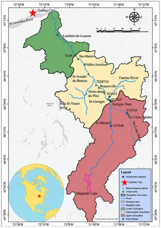
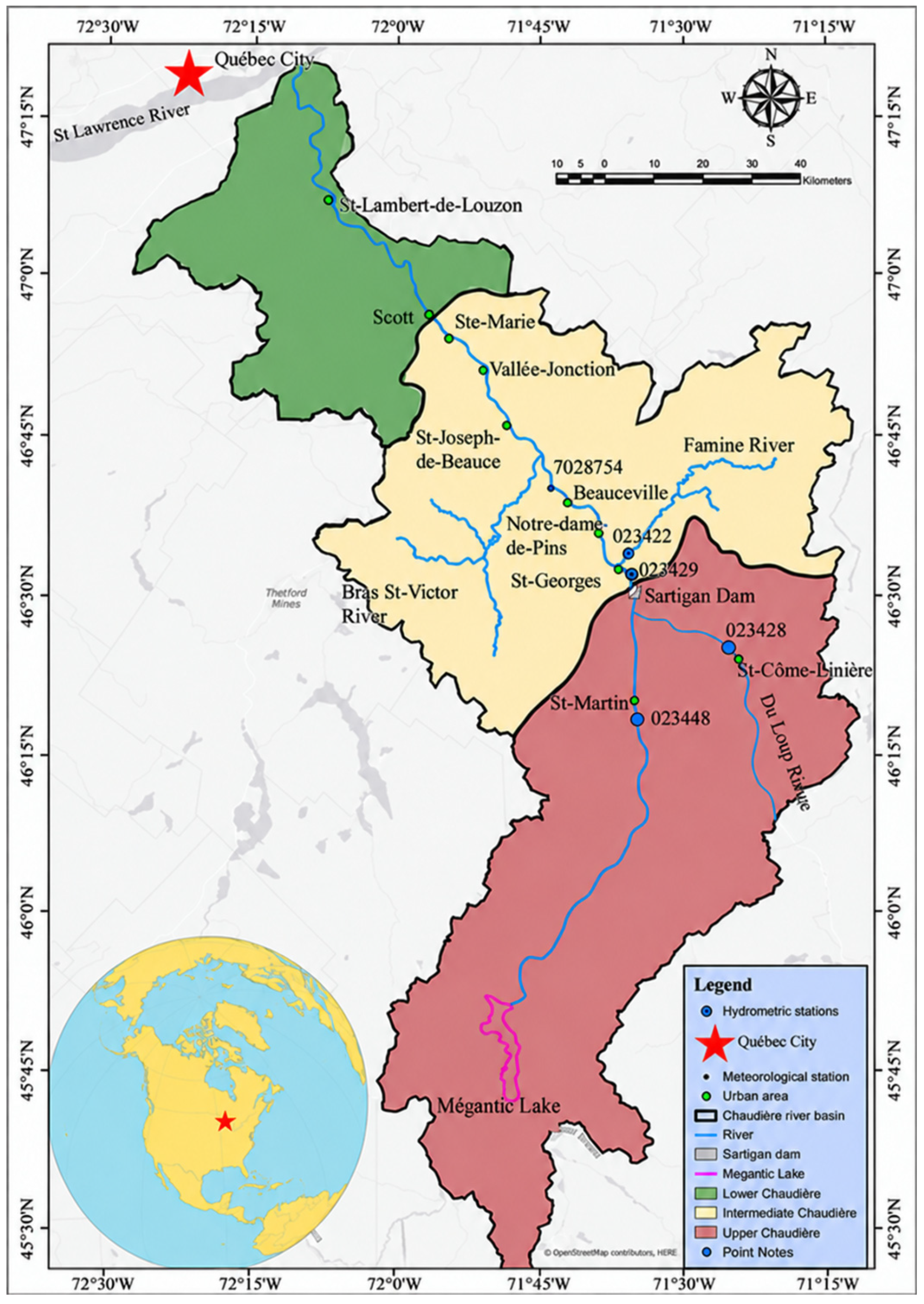
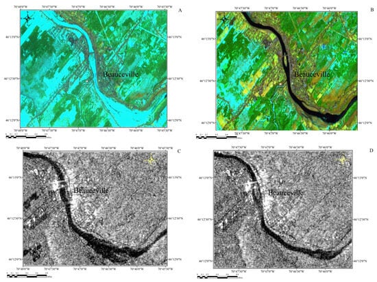
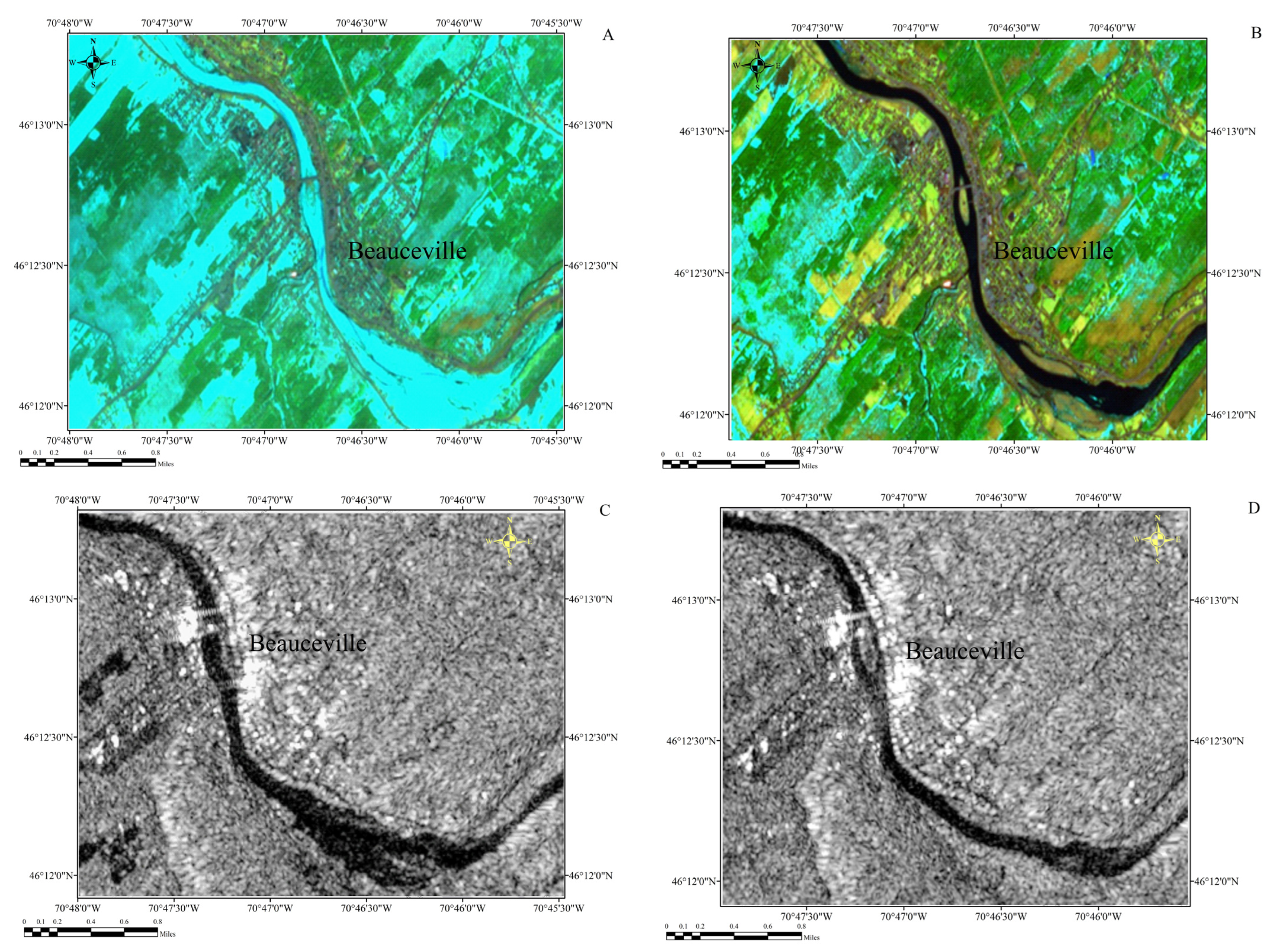
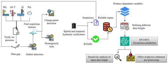
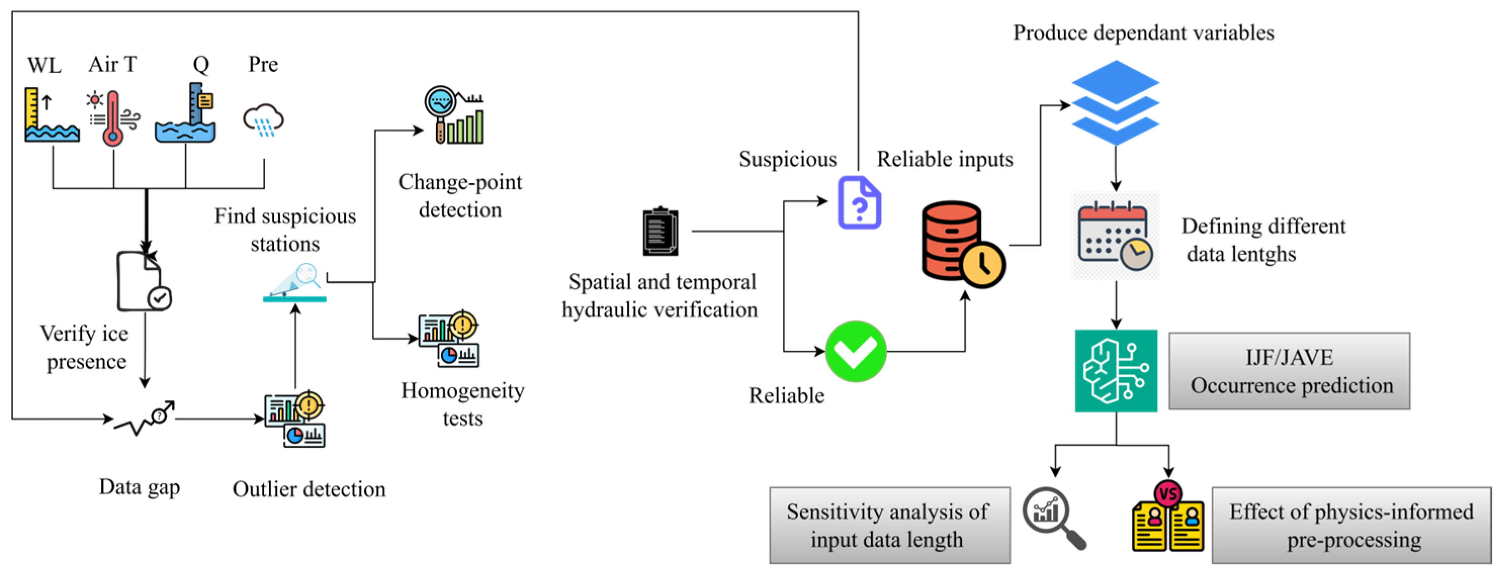
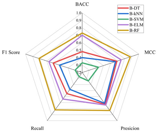
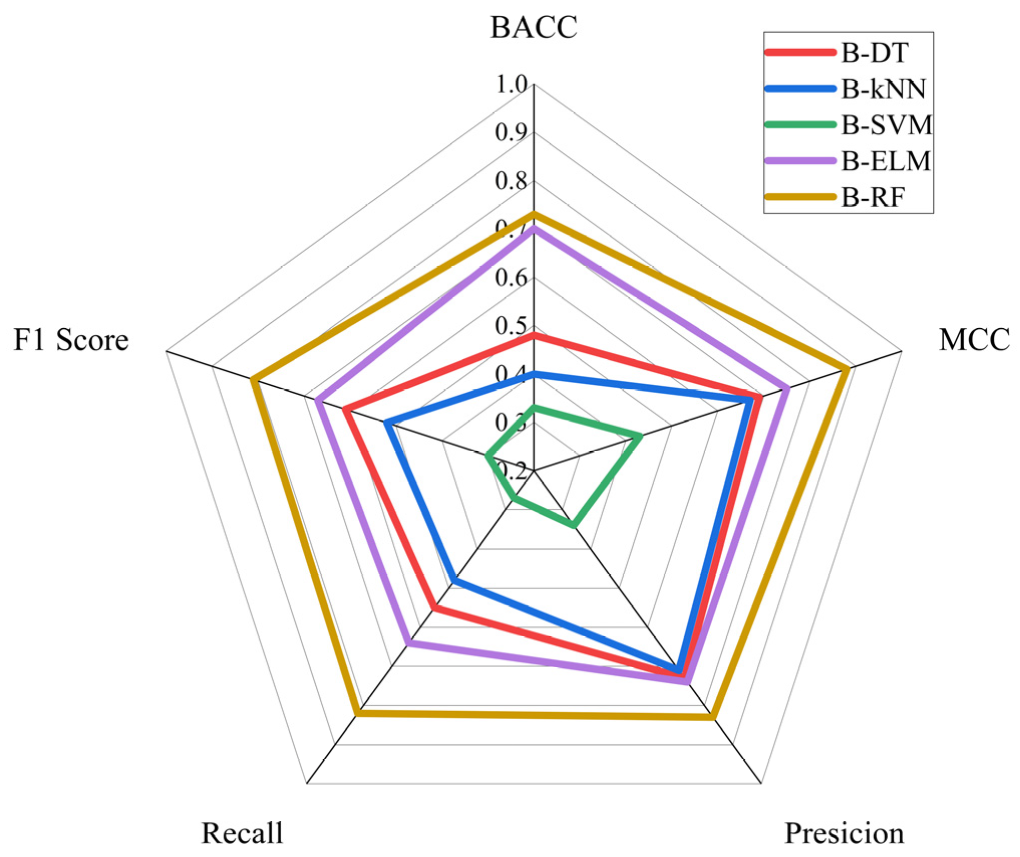
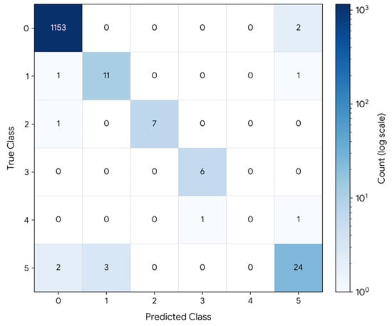
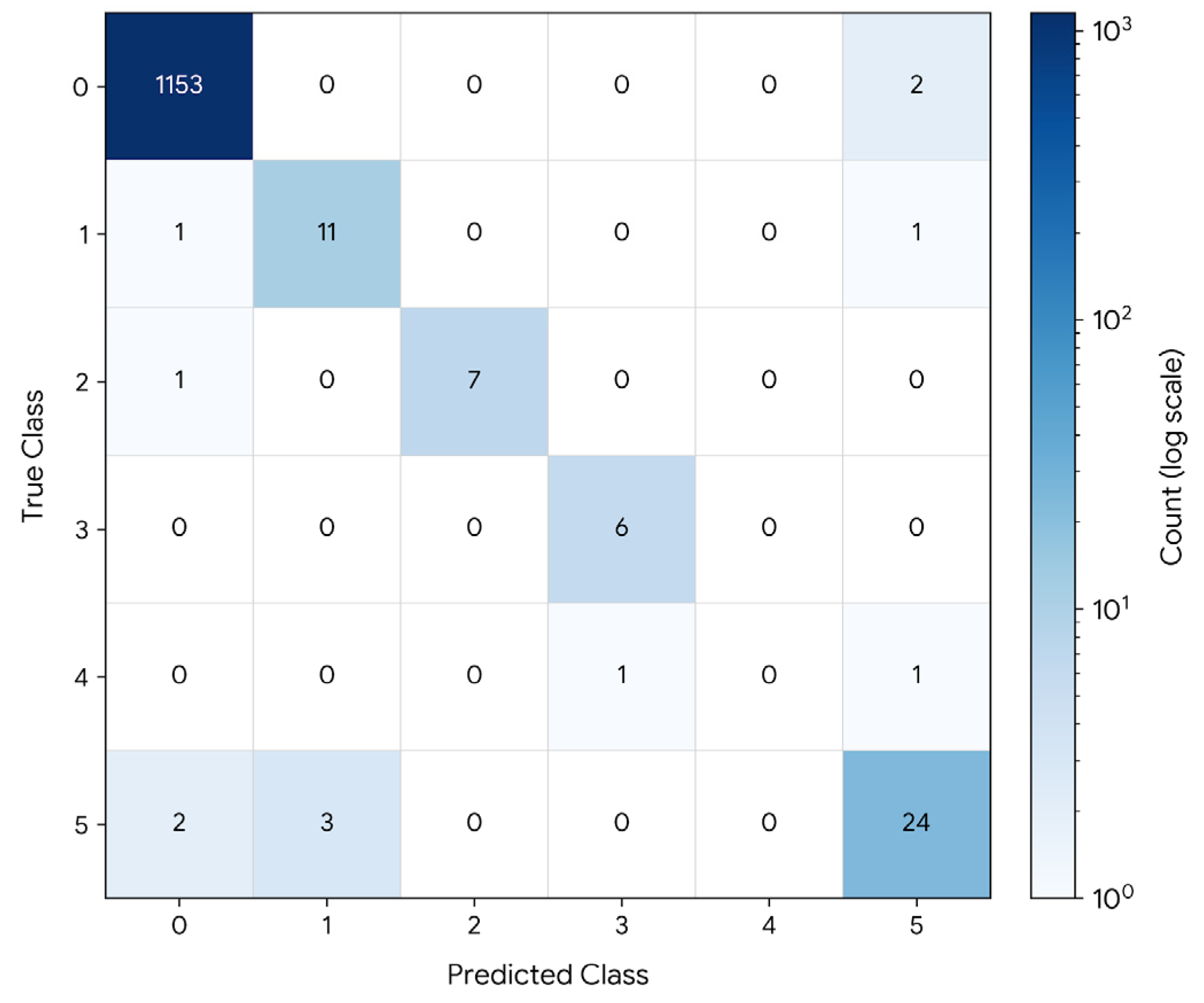
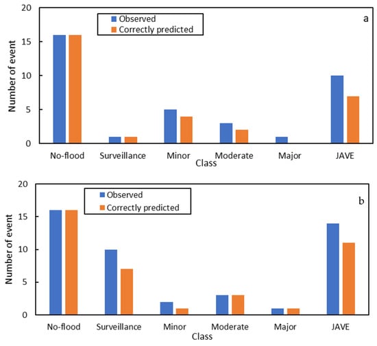
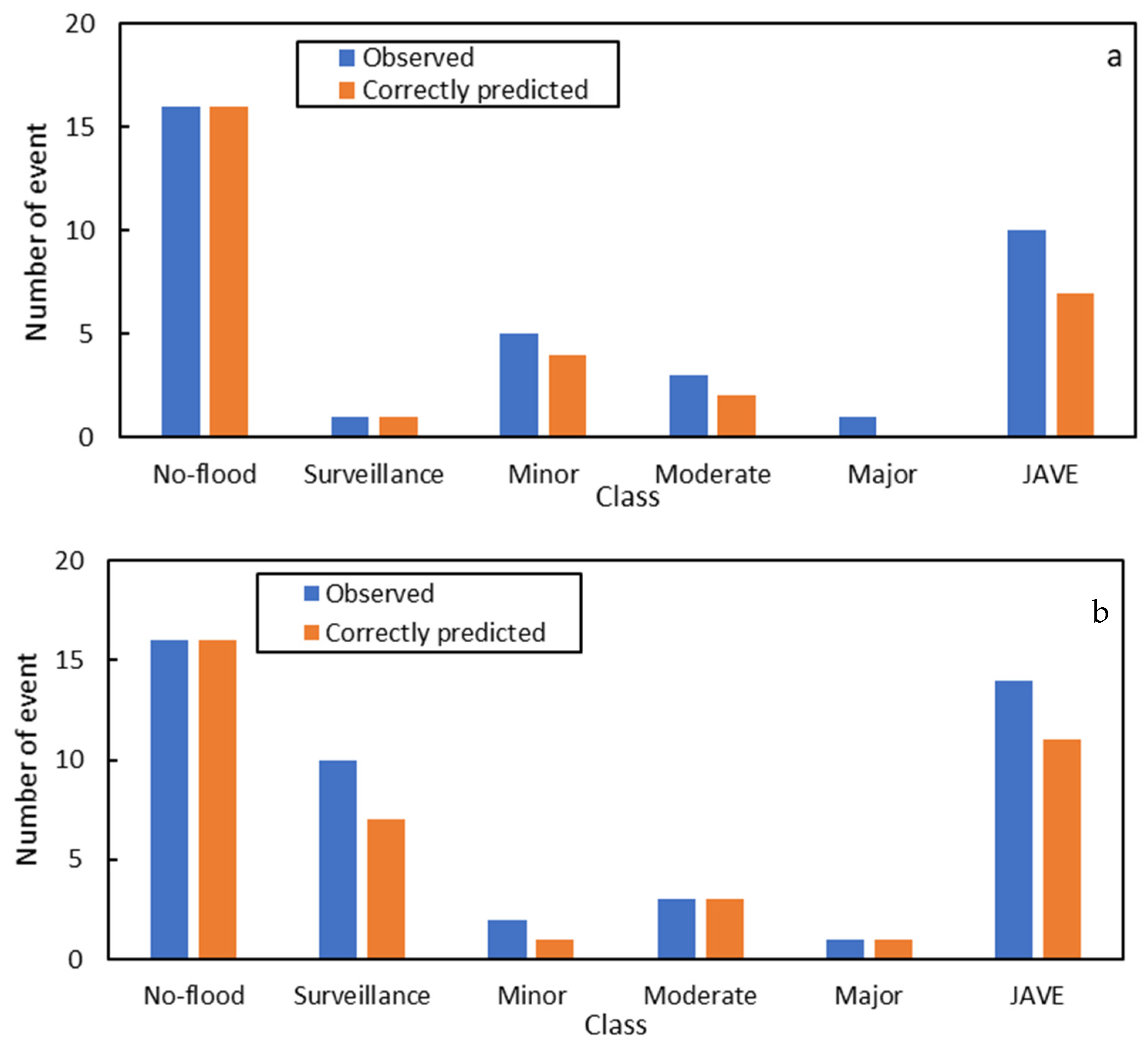
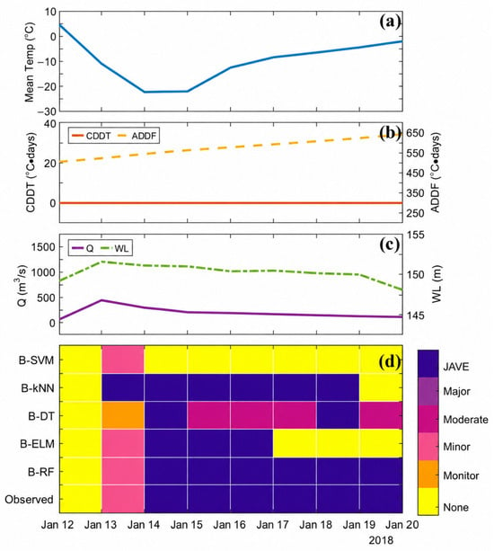
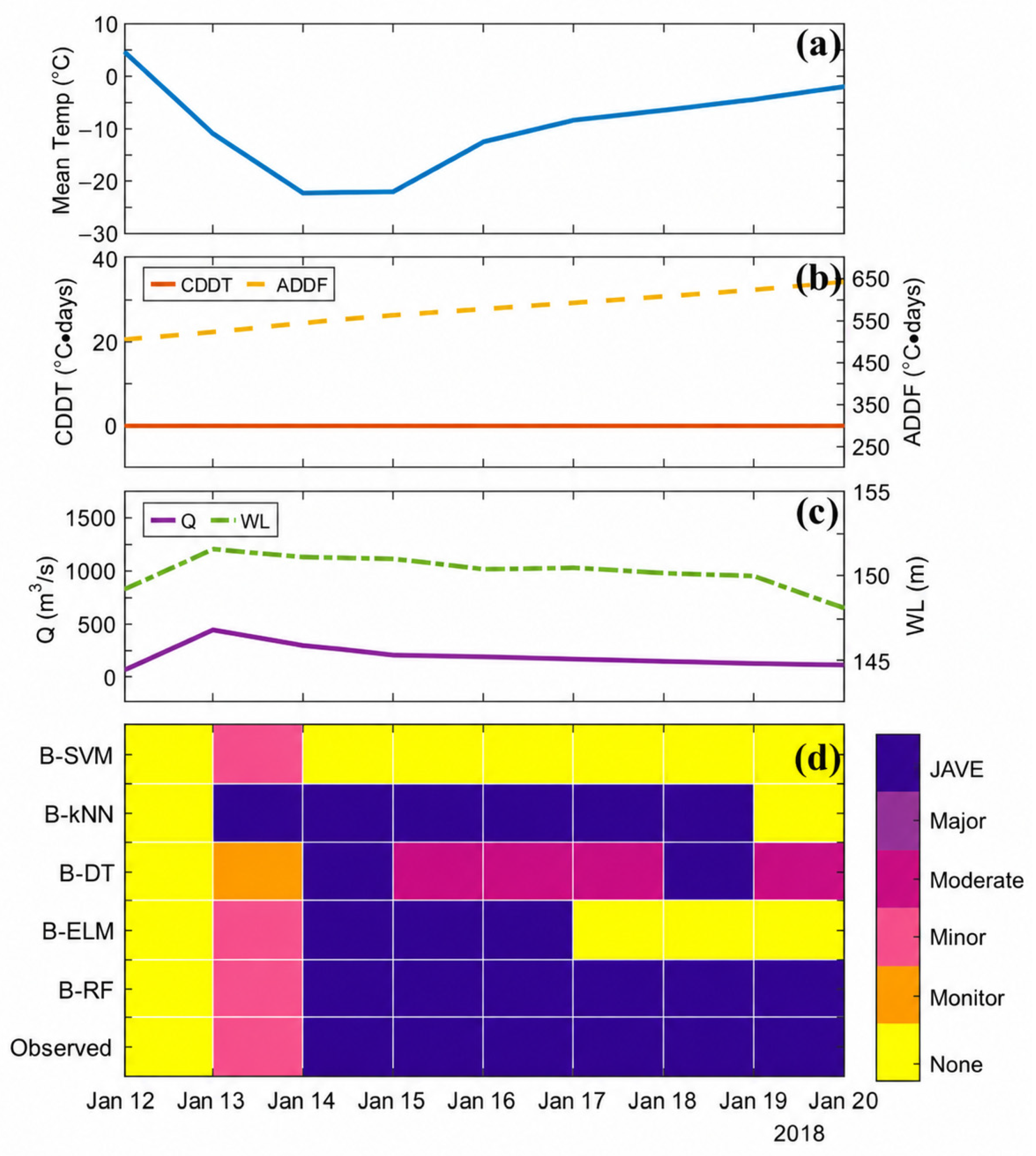
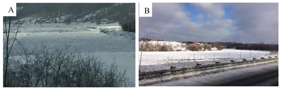
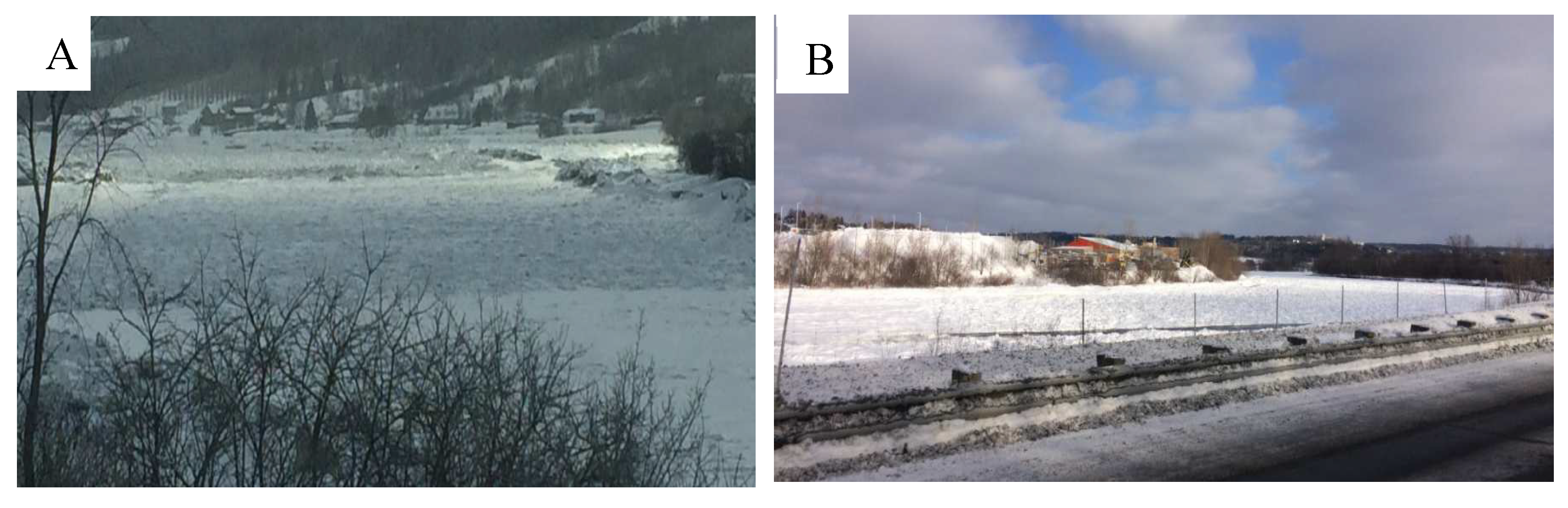
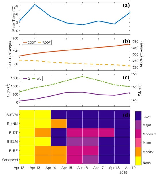
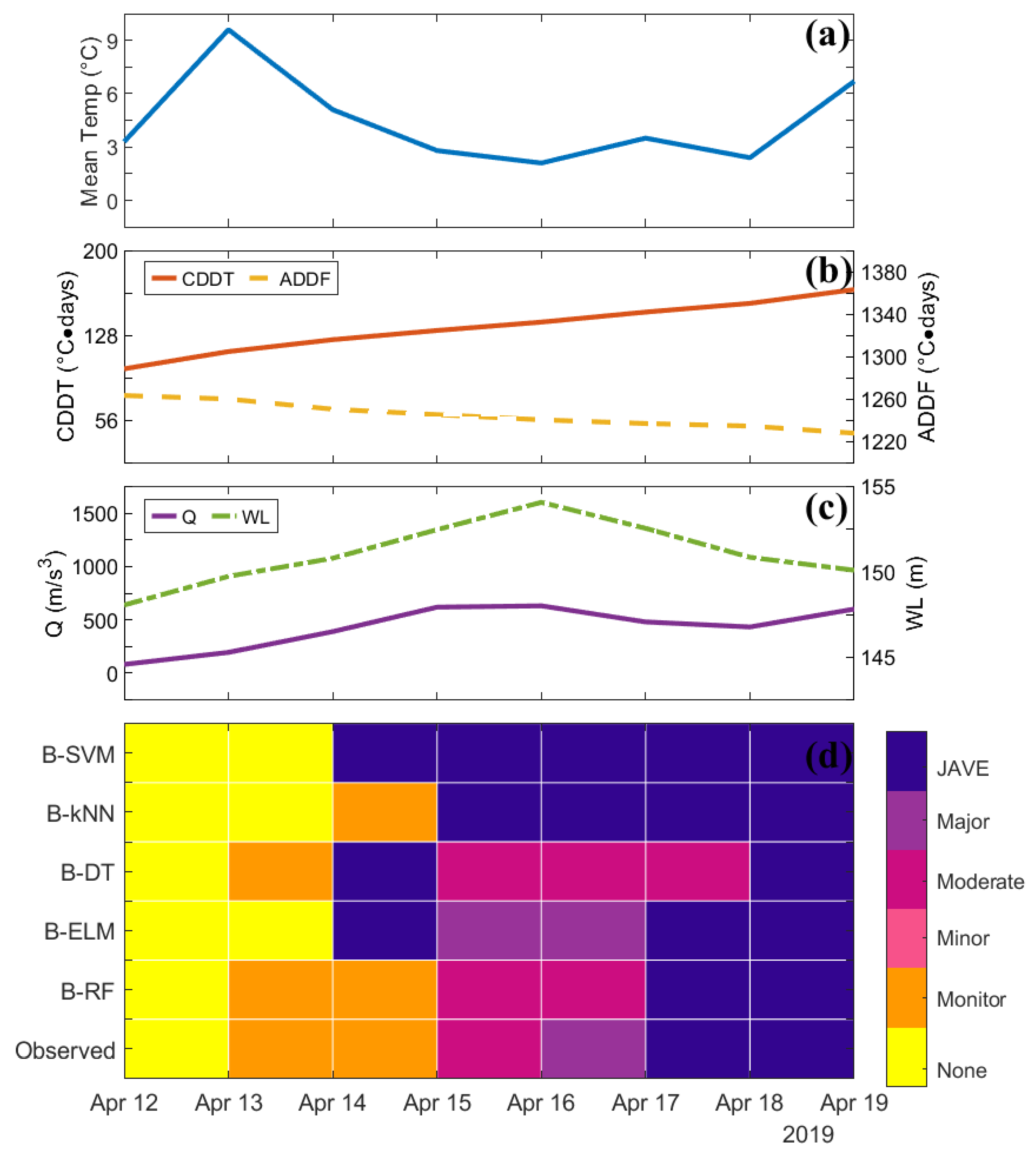
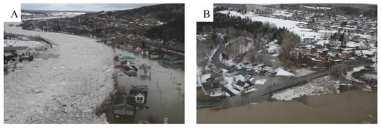
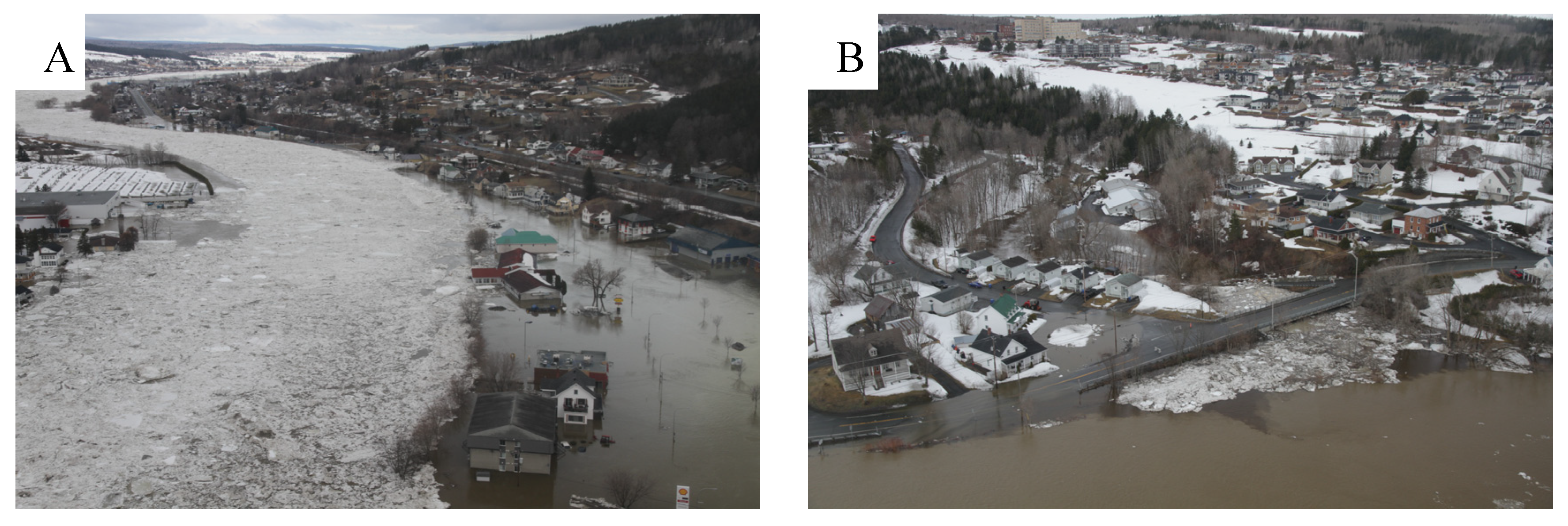
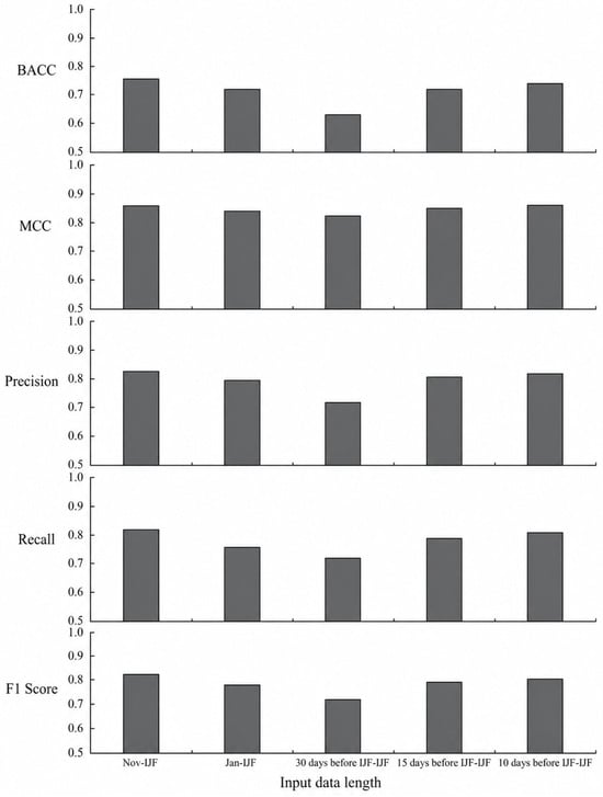
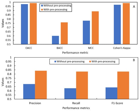

Disclaimer/Publisher’s Note: The statements, opinions and data contained in all publications are solely those of the individual author(s) and contributor(s) and not of MDPI and/or the editor(s). MDPI and/or the editor(s) disclaim responsibility for any injury to people or property resulting from any ideas, methods, instructions or products referred to in the content. |
© 2026 by the authors. Licensee MDPI, Basel, Switzerland. This article is an open access article distributed under the terms and conditions of the Creative Commons Attribution (CC BY) license.