Coupled Sustainable Management Zoning of Ecological Vulnerability and Soil Erosion in the Eastern Dabie Mountains

Abstract

Mountain–hill–plain transition zones combine terrain sensitivity, agricultural land use, and construction pressure and therefore require spatially differentiated management. This study develops a pressure-oriented framework that distinguishes composite ecological vulnerability from soil-erosion pressure and translates their multi-period co-occurrence into management demand. Using multi-source raster data for 2000, 2005, 2010, 2015, and 2020 on a common 30 m reference grid, we constructed an ecological vulnerability index (EVI) from 14 ecological, environmental, and human-activity indicators using a sensitivity–resilience–pressure framework, combined analytic hierarchy process (AHP)–entropy weighting, and unified natural breaks. Soil erosion intensity was estimated with the Revised Universal Soil Loss Equation (RUSLE) using digital elevation model (DEM)-derived flow accumulation, a capped effective slope length, and a fractional vegetation cover (FVC)-based cover-management factor. The EVI and RUSLE dimensions were integrated through a two-dimensional pressure matrix, a Coupled Pressure Index (CPI), and an Integrated Management Demand Index (IMDI). High vulnerability was concentrated in northern, urban-fringe, and selected agricultural areas, whereas moderate-or-above erosion was concentrated on slopes, in gullies, and on hilly farmland; areas subject to both pressures were spatially selective. The largest EVI weights were assigned to mean annual precipitation (0.3841), mean annual temperature (0.1727), ecosystem type (0.0820), biological abundance (0.0810), and built-up land ratio (0.0746). Non-vulnerable and slightly vulnerable areas increased from 40.62% to 64.27%, whereas highly and extremely vulnerable areas decreased from 38.98% to 23.29%. Moderate-or-above soil erosion accounted for 13.56% in 2020. The five-zone comprehensive management classification comprised stable conservation (40.19%), soil and water conservation priority (13.73%), ecological vulnerability regulation (27.94%), integrated management priority (1.48%), and transition management (16.66%). By linking ecological diagnosis, erosion-pressure identification, persistence analysis, and county-level zoning, the framework provides an interpretable spatial basis for prioritizing ecological conservation, soil and water conservation, and land-use management in mountain–hill–plain transition regions.

1. Introduction

Ecological vulnerability assessment connects ecosystem diagnosis with spatial management decisions. The vulnerability framework proposed by Turner et al. explains regional risk as the result of interactions among external disturbance, system sensitivity, and response capacity [1]. This process-oriented perspective is important for sustainable land management because a high vulnerability score may result from different combinations of natural sensitivity, limited ecological resilience, and human pressure. A useful assessment should therefore identify both the composite vulnerability pattern and the specific processes requiring intervention.

Mountain–hill–plain transition regions are particularly difficult to assess because terrain, climate, land cover, agricultural use, and socioeconomic activity can change sharply over short distances. Adger’s definition of vulnerability emphasizes both potential harm under stress and the capacity to adapt [2]. In these regions, ecological vulnerability is not equivalent to soil erosion: a location may be vulnerable because of climatic or ecosystem constraints while experiencing limited erosion, whereas a sloping agricultural or disturbed area may experience strong erosion pressure without belonging to the highest vulnerability class. Treating these dimensions as distinct but spatially comparable is essential for differentiated management.

A multi-indicator index is needed to represent these interacting conditions. The analytic hierarchy process translates expert knowledge about indicator importance into structured weights [3], whereas entropy weighting incorporates the spatial information content and dispersion of the observed data [4]. For an EVI constructed from 14 indicators, combining AHP and entropy weighting is appropriate when the indicator directions, classification scheme, spatial resolution, and treatment of static background variables and time-varying variables are clearly specified. The resulting EVI should therefore be interpreted as a relative composite assessment of ecological vulnerability rather than a direct observation of ecological state.

Soil erosion is a distinct process dimension with direct implications for soil and water conservation. The Revised Universal Soil Loss Equation (RUSLE) estimates the annual water-erosion modulus from rainfall erosivity, soil erodibility, slope length and steepness, cover-management, and support-practice factors [5]. Land use and climate change can substantially alter erosion risk [6], and terrain-mediated erosion may not follow the same spatial pattern as composite ecological vulnerability. RUSLE should therefore enter the management analysis as an independent pressure layer, with its factor assumptions, grid alignment, and regional-scale interpretation stated explicitly.

Previous studies have demonstrated the usefulness of AHP–entropy frameworks for mapping ecological vulnerability [7]. VSD and PSR frameworks have also been applied to represent vulnerability as an interaction among pressure, sensitivity, and response capacity [8]. Related composite assessments have combined indicator weighting and spatial classification to support ecological management [9]. However, two gaps remain. First, many composite vulnerability assessments do not retain soil erosion as an independently evaluated process, which can obscure the distinction between ecosystem vulnerability and the need for slope-runoff, gully, and soil-conservation interventions. Second, studies that combine ecological vulnerability with erosion commonly emphasize a single-period overlay, providing limited evidence of whether a priority location is persistent or reflects only a temporary condition.

A further methodological issue is how continuous indices are converted into classes that are meaningful for management. Jenks natural breaks can reduce within-class variation and emphasize between-class differences [10], but classification rules should serve comparability rather than be presented as causal evidence. Geodetector can quantify spatially stratified heterogeneity and correspondence between factor patterns [11]; however, this study uses Spearman’s rho and Cramér’s V because its primary statistical objective is to characterize the association between two ordinal pressure layers. Identifying driving factors is outside the scope of this study, and Geodetector analysis was therefore not performed. Multi-period frequencies and sensitivity scenarios were used to examine whether priority zones remain stable under alternative assumptions. These considerations motivate a pressure-matrix approach that separates annual diagnosis from long-term management demand.

The eastern Dabie Mountains provide a suitable case for addressing these gaps. The region combines important ecological-barrier and water-conservation functions with sloping farmland, expansion along transport corridors and urban fringes, and a transition from mountainous and hilly terrain to river–lake plains. Remote-sensing indicators have been used to describe ecological-environmental change in the Dabie Mountain area [12], but a single composite index cannot by itself distinguish ecosystem vulnerability, soil and water conservation pressure, and land-use control demand.

Sustainable land management requires spatial coordination among ecosystem conditions, ecological processes, and socioeconomic needs. Existing research on ecological restoration and security patterns emphasizes ecosystem services, landscape connectivity, ecological sources, corridors, and implementable restoration units [13]. Research on ecological security-pattern optimization likewise highlights the need to translate restoration objectives into spatially implementable units [14]. Building on this perspective, this study uses EVI and RUSLE-derived soil-erosion intensity as complementary dimensions. It combines an explicit two-dimensional pressure matrix with a Coupled Pressure Index (CPI) and an Integrated Management Demand Index (IMDI) that incorporates current pressure, multi-period mean pressure, and annual priority frequency.

Accordingly, this study addresses three research questions: (Q1) How did the 14-indicator EVI and RUSLE-derived soil-erosion intensity change spatially and temporally from 2000 to 2020 in the eastern Dabie Mountains? (Q2) Do ecological vulnerability and soil-erosion pressure occur synchronously, or do they represent distinct spatial processes? (Q3) How can their annual overlay and multi-period persistence be translated into robust management zones and differentiated county-level actions? To answer these questions, we aim to: (1) construct comparable five-period EVI and RUSLE datasets on a common 30 m analysis grid; (2) quantify their cross-year relationship using pressure matrices and statistical association measures; and (3) develop and evaluate annual and comprehensive management zoning using CPI, IMDI, frequency information, county overlays, and weight-sensitivity scenarios. The main contributions are the explicit separation of vulnerability from erosion pressure, the translation of multi-period pressure persistence into a management-demand index, and systematic checks of terrain consistency, resampling effects, and zoning robustness in a mountain–hill–plain transition region.

2. Materials and Methods

2.1. Study Area

The study area comprises selected county-level units within Lu’an and Anqing cities, Anhui Province. It extends from approximately 29°47′ to 32°36′ N and 115°22′ to 117°15′ E and covers about 29,000 km². The area lies in the eastern section of the Qinling–Dabie Mountains ecological barrier and contains mountains, hills, low uplands, river–lake plains, and urban fringes. Terrain generally descends from the northwestern mountains toward the southeastern plains. DEM-derived elevation has a mean of 211.29 m, a median of 64.00 m, and a 95th percentile of 787.00 m; the mean slope is 11.63°, the median slope is 7.16°, and 40.92% of the analysis area has slopes of at least 10°. These gradients make the region suitable for distinguishing terrain-mediated erosion pressure from broader ecological vulnerability.

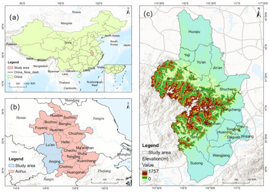
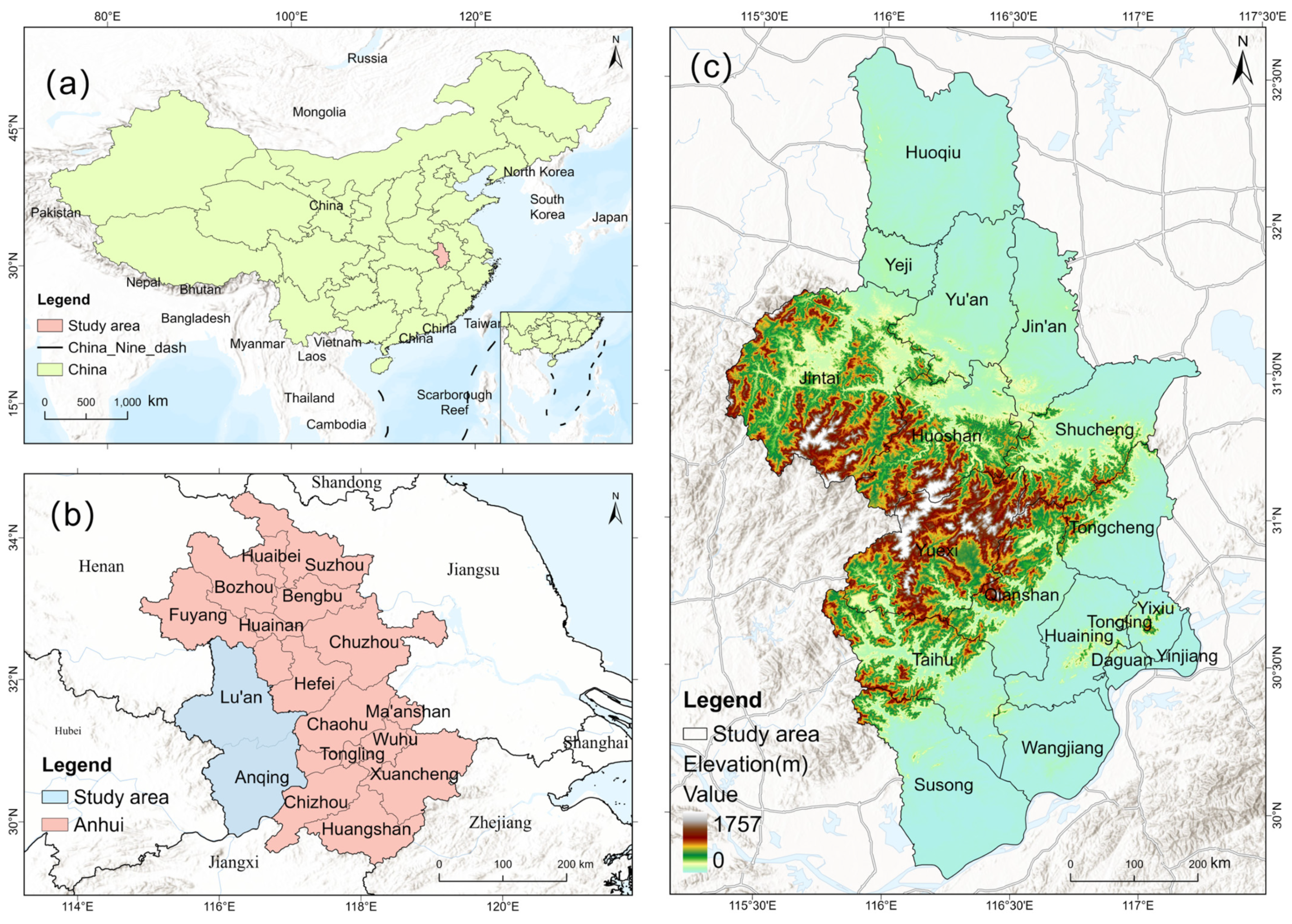
The region has a northern subtropical humid monsoon climate with favorable hydrothermal conditions, but precipitation is seasonally concentrated and can generate runoff erosion on local slopes and in gullies. The 2020 land-use cross-check indicates that cropland accounts for 51.38% of the valid area; forest, grassland, and shrubland together account for 39.62%; water accounts for 5.60%; and built-up land accounts for 3.40%. The mapped soil units include paddy soils, Luvisols, Ferralsols, Primisols, and Skeletal soils, providing a heterogeneous background for the soil-erodibility factor. Mountainous and hilly areas provide important ecological-barrier functions, whereas plains and urban fringes concentrate agricultural production, population activity, and construction expansion. Land-use types also include localized mining, quarrying, and other construction-disturbed patches that may expose soil and alter runoff pathways. This combination of steep terrain, extensive cropland, heterogeneous soils, disturbance patches, and urban–rural transition means that management demand cannot be inferred from a single vulnerability class. The location, administrative divisions, and topographic background of the study area are shown in Figure 1.

Figure 1. Location and topographic background of the study area. (a) Location in China; (b) location in Anhui Province; and (c) selected county-level study domain with elevation background. The elevation background was derived from the static ASTER GDEM V2 product at 30 m resolution [15], reprojected to CGCS 2000/EPSG:4548, aligned with the common 30 m reference grid, and clipped to the study domain. The archived DEM does not encode a single acquisition year and was therefore treated as a static topographic layer throughout the period 2000–2020. The boundary source is the 2020 national county-level administrative division dataset; the boundary layer used in this study was selected and adapted to the Lu’an–Anqing analysis units. Locator and county-boundary layers were used for cartographic overlay. The map was prepared using ArcGIS Pro (v3.1.5), Python (v3.12), rasterio (v1.5.0), GeoPandas (v1.1.3), and Matplotlib (v3.10.8). Boundaries are used solely for cartographic presentation and do not imply any territorial claim or boundary endorsement by the authors or publisher.

2.2. Analytical Methods

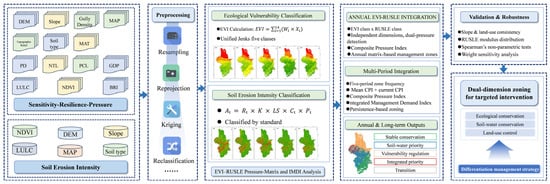
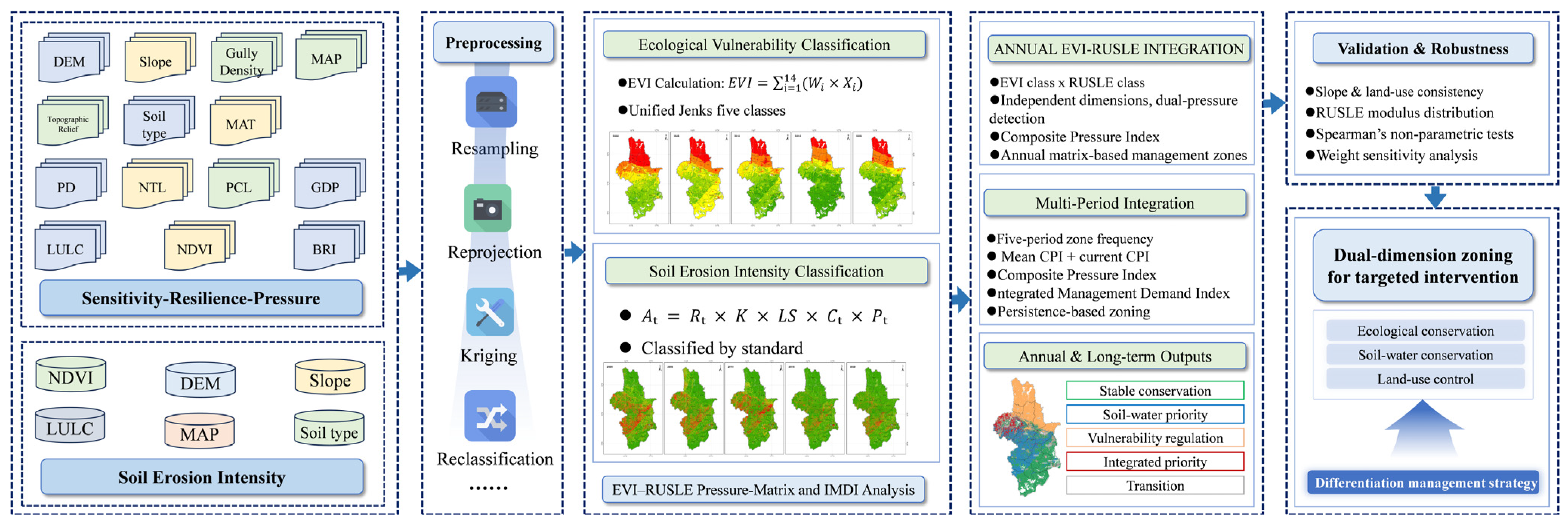
The study followed seven steps: data preprocessing and multi-resolution alignment; ecological vulnerability calculation; soil-erosion estimation; annual EVI–RUSLE pressure zoning; comprehensive management zoning; validation and sensitivity analysis; and result interpretation (see Figure 2). First, the 14 indicators, including elevation, slope, gully density, climate, vegetation, ecosystem type, population and economic activity, and built-up land, were classified on a common scale and aligned to the same raster grid. Second, AHP–entropy combined weighting was used to calculate EVI for the five periods, and unified natural breaks were used to classify the results as non-vulnerable, slightly vulnerable, moderately vulnerable, highly vulnerable, or extremely vulnerable. Third, RUSLE soil-erosion intensity was estimated using DEM-derived flow accumulation and an FVC-based cover-management factor. Annual EVI–RUSLE pressure zones were then derived from an explicit two-dimensional matrix, and comprehensive management zones were delineated using five-period zone frequencies, CPI, IMDI, and county-level administrative overlays. Finally, terrain and land-use consistency checks, statistical association tests, and alternative-weight scenarios were used to assess the plausibility and robustness of the results.

Figure 2. Research workflow for the five-period EVI–RUSLE analysis. The workflow combines analytic hierarchy process–entropy weighting and a geospatial raster workflow using rasterio (v1.5.0), GeoPandas (v1.1.3), NumPy (v2.4.1), SciPy (v1.17.1), and Matplotlib (v3.10.8), together with a common 30 m reference grid for preprocessing, EVI/RUSLE classification, pressure-matrix analysis, IMDI integration, validation, and management zoning. Abbreviations: DEM, digital elevation model; MAP, mean annual precipitation; MAT, mean annual temperature; PD, population density; NTL, nighttime light; PCL, proportion of construction land (built-up land ratio); GDP, gross domestic product; LULC, land use/land cover; NDVI, normalized difference vegetation index; BRI, biological resource index (biological abundance index); EVI, ecological vulnerability index; RUSLE, Revised Universal Soil Loss Equation; LS, slope-length and steepness factor; R, rainfall erosivity; K, soil erodibility; C, cover-management factor; P, support-practice factor; CPI, Coupled Pressure Index; IMDI, Integrated Management Demand Index.

2.3. Data Sources and Preprocessing

Five periods—2000, 2005, 2010, 2015, and 2020—were selected. Source rasters and their corresponding classified 30 m indicator rasters were prepared on the common analysis grid. The 14 EVI indicators were elevation, slope, gully density, relief amplitude, soil type, mean annual temperature, mean annual precipitation, normalized difference vegetation index (NDVI), biological abundance index, ecosystem type, population density, gross domestic product (GDP) density, nighttime light index, and built-up land ratio. The DEM was obtained from the ASTER Global Digital Elevation Model Version 2 (ASTER GDEM V2) and used to derive slope, gully density, and relief amplitude [15]. Soil type was derived from the Second National Soil Survey of China [16]. Ecosystem type and built-up land ratio were extracted from the China Land Cover Dataset (CLCD) [17]. Table 1 summarizes the spatial resolution and source of each input layer. Annual summaries of the raw input variables—including units, temporal status, and mean ± standard deviation before EVI scoring—are reported in Appendix A, Table A6; the composition of categorical soil and ecosystem inputs is reported in Appendix A, Table A7.

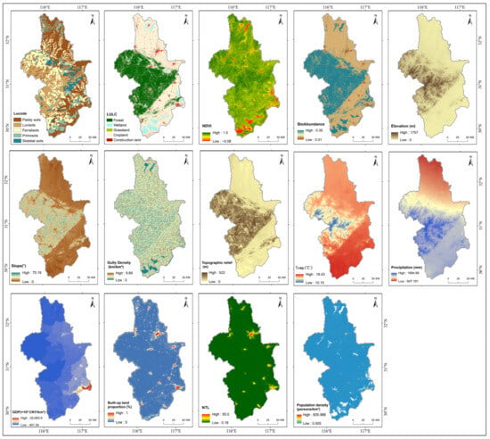
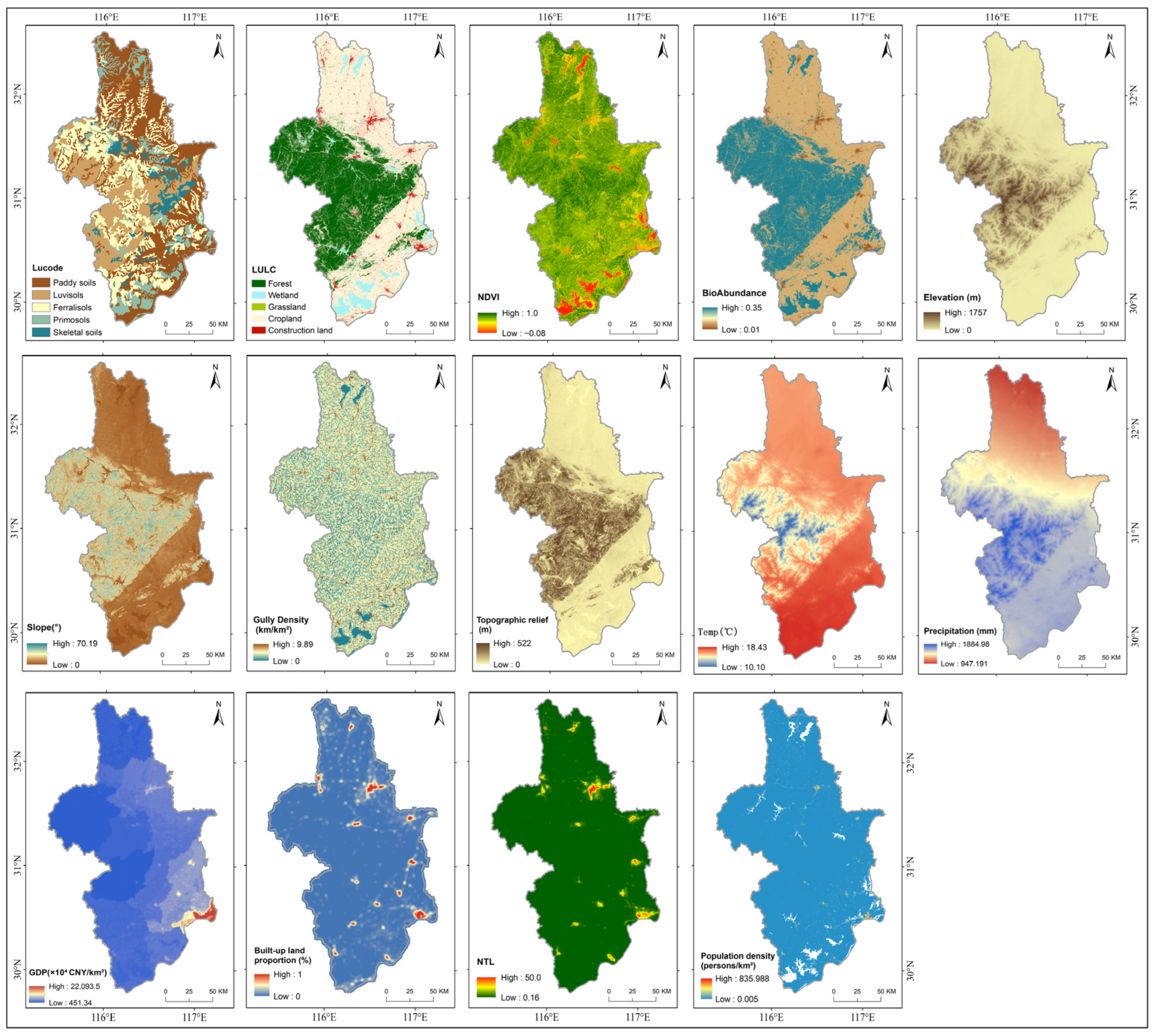
Figure 3 presents the spatial distributions of the 14 indicators used to construct EVI in 2020; inputs from all five periods were used for the subsequent temporal analysis. The sensitivity dimension includes elevation, slope, gully density, relief amplitude, soil type, mean annual temperature, and mean annual precipitation; higher grades indicate stronger natural sensitivity or climatic constraint. The resilience dimension includes NDVI, biological abundance, and ecosystem type. These indicators were directionally standardized so that higher grades consistently represent greater vulnerability; consequently, stronger vegetation or ecosystem resilience receives a lower vulnerability grade before weighting. The pressure dimension includes population density, GDP density, nighttime light, and built-up land ratio; higher values indicate stronger human-disturbance pressure. The static indicators were elevation, slope, gully density, relief amplitude, and soil type. The dynamic indicators were mean annual temperature, mean annual precipitation, NDVI, biological abundance, ecosystem type, population density, GDP density, nighttime light, and built-up land ratio, which were entered for each selected period when year-specific data were available. The land-use/land-cover raster was an independent RUSLE input and was also used to derive ecosystem type and the built-up land ratio. The figure therefore shows both the spatial complementarity of the 14 indicators and the basis for their role-specific standardization. Annual valid-area means of the classified input scores are reported in Table S5, and the direction and grading rules are listed in Table S6. Raw annual values are reported in Appendix A, Table A6, whereas Table S5 reports the annual means of the classified scores actually entering the EVI calculation.

Figure 3. Spatial distributions of the 14 indicators used for ecological vulnerability assessment in 2020. The panels show elevation, slope, gully density, topographic relief, biological abundance, soil type, temperature, precipitation, NDVI, GDP density, land use/land cover, population density, nighttime light, and built-up land proportion. Continuous variables are shown as gradients, whereas categorical variables are shown as classes.

Temperature and precipitation data were obtained from the 1 km monthly climate dataset for China and aggregated into mean annual temperature and annual precipitation for each study year [18]. NDVI was generated in Google Earth Engine using annual maximum-value composites from Landsat imagery [19]. The long-term 30 m Landsat observation record provides the basis for extracting multi-period vegetation and land-cover information [20]. The biological abundance index was calculated from ecosystem-type weights following HJ 192-2015 [21]. Population density was obtained from the WorldPop open gridded population dataset [22]. GDP density was obtained from China’s GDP spatial-distribution kilometer-grid dataset [23]. The nighttime-light index was derived from a harmonized cross-sensor DMSP/OLS and NPP-VIIRS dataset [24].

All source rasters were checked for their coordinate reference system, extent, pixel size, transform, and missing-data conventions. Continuous quantitative variables—including precipitation, temperature, DEM-derived surfaces, soil erodibility, NDVI, population, GDP, and nighttime light—were aligned using bilinear interpolation. Categorical variables—including soil type, ecosystem type, and land-use/land-cover classes—were aligned using nearest-neighbor resampling so that class codes were not averaged. The resulting layers were written or read on the common 30 m reference grid used for the EVI–RUSLE overlay. For the 1 km climate and socioeconomic inputs, this operation represents spatial interpolation of a coarse background field; it does not create independent 30 m information. Accordingly, the 30 m outputs are interpreted as relative spatial-prioritization maps, and fine-scale boundaries should not be regarded as observations at 30 m precision.

Soil-erosion intensity was calculated with the RUSLE equation and its five factors. Rainfall erosivity was derived from annual precipitation, soil erodibility was assigned according to soil type, and the slope-length and steepness factor was calculated from DEM-derived slope and flow-length information. The cover-management factor was estimated from NDVI and land-cover information, whereas the support-practice factor was assigned according to land-use and conservation-practice classes. The five factors were multiplied on the common 30 m grid to obtain the annual erosion modulus, which was then entered into the coupling analysis as ranked classes. Erosion classes were coded as 1, 3, 5, 7, and 9 and divided into slight, light, moderate, strong, and very strong-and-above erosion according to the Classification and Gradation Standard of Soil Erosion [25]. All rasters were aligned to the same projection, resolution, and pixel grid to ensure pixel-by-pixel comparability among EVI, soil-erosion intensity, and management zoning.

For the revised RUSLE calculation, precipitation, K, and NDVI were aligned to the reference grid using bilinear interpolation, whereas land use was aligned using nearest-neighbor resampling. DEM-based terrain and flow-length calculations were retained on the 30 m reference framework. This explicit separation between continuous and categorical resampling avoids artificial class mixtures and prevents overstatement of the spatial detail provided by coarse inputs.

Data preprocessing comprised two key steps. First, all indicators were assigned a common grading direction, so that higher grades represented stronger contributions to vulnerability and the weighted overlay had a consistent interpretation. Second, static and dynamic indicators were treated separately: static indicators remained unchanged across the five periods, whereas dynamic indicators were entered for their corresponding years. Temporal changes therefore primarily reflected period-specific variation in vegetation, ecosystem structure, socioeconomic pressure, built-up land ratio, and climatic background.

Table 1. Data sources.

Indicator	Spatial Resolution	Data Source
Elevation (DEM)	30 m	Geospatial Data Cloud, ASTER GDEM V2 [15]
Slope	30 m	Derived from DEM [15]
Gully density	30 m	Derived from DEM hydrological analysis [15]
Relief amplitude	30 m	Derived from DEM [15]
Soil type	Vector	Second National Soil Survey of China [16]
Ecosystem type (land cover)	30 m	CASEarth thematic data system, China Land Cover Dataset (CLCD, 1985–2024) [17]
Mean annual temperature	1 km	National Tibetan Plateau Data Center/Third Pole Environment Data Center 1 km climate dataset [18]
Annual precipitation	1 km	National Earth System Science Data Center 1 km climate dataset [18]
NDVI	30 m	Google Earth Engine, Landsat annual maximum-value composite [19]
Biological abundance	30 m	Weighted synthesis based on ecosystem type following HJ 192–2015 [21]
Population density	100 m	Google Earth Engine, WorldPop dataset [22]
GDP grid	1 km	RESDC, China’s GDP spatial distribution kilometer-grid dataset [23]
Nighttime light index	1 km/500 m	Google Earth Engine, cross-sensor harmonized DMSP/OLS and NPP-VIIRS nighttime light data [24]
Built-up land ratio	30 m	Extracted from CLCD land-cover data using 90 m neighborhood statistics [17]
Soil erosion intensity	30 m	Calculated using RUSLE

Table 1. Data sources.

Indicator	Spatial Resolution	Data Source
Elevation (DEM)	30 m	Geospatial Data Cloud, ASTER GDEM V2 [15]
Slope	30 m	Derived from DEM [15]
Gully density	30 m	Derived from DEM hydrological analysis [15]
Relief amplitude	30 m	Derived from DEM [15]
Soil type	Vector	Second National Soil Survey of China [16]
Ecosystem type (land cover)	30 m	CASEarth thematic data system, China Land Cover Dataset (CLCD, 1985–2024) [17]
Mean annual temperature	1 km	National Tibetan Plateau Data Center/Third Pole Environment Data Center 1 km climate dataset [18]
Annual precipitation	1 km	National Earth System Science Data Center 1 km climate dataset [18]
NDVI	30 m	Google Earth Engine, Landsat annual maximum-value composite [19]
Biological abundance	30 m	Weighted synthesis based on ecosystem type following HJ 192–2015 [21]
Population density	100 m	Google Earth Engine, WorldPop dataset [22]
GDP grid	1 km	RESDC, China’s GDP spatial distribution kilometer-grid dataset [23]
Nighttime light index	1 km/500 m	Google Earth Engine, cross-sensor harmonized DMSP/OLS and NPP-VIIRS nighttime light data [24]
Built-up land ratio	30 m	Extracted from CLCD land-cover data using 90 m neighborhood statistics [17]
Soil erosion intensity	30 m	Calculated using RUSLE

2.4. Calculation and Classification of Ecological Vulnerability and Soil-Erosion Intensity

The EVI was constructed using a sensitivity–resilience–pressure framework. The sensitivity layer included elevation, slope, gully density, relief amplitude, soil type, mean annual temperature, and mean annual precipitation. The resilience layer included NDVI, the biological abundance index, and ecosystem type. The pressure layer included population density, GDP density, the nighttime-light index, and the built-up land ratio. These 14 indicators were used to calculate EVI, whereas soil-erosion intensity was treated as an independent dimension in the subsequent pressure-overlay analysis. For continuous dynamic indicators, one five-year pooled-mean raster was classified for each indicator using a five-class Jenks natural-breaks procedure, and the resulting four breakpoints were applied to all selected years. The original GIS processing retained the final score rasters but did not preserve the numeric breakpoint table; therefore, the breakpoint notation and score mapping are documented in Table S6 without reconstructing unverified constants.

AHP weights were used to represent the relative importance of indicators, and entropy weights were used to represent the overall spatial dispersion of the five-period indicator data. To ensure comparability of EVI from 2000 to 2020, the two weighting components were combined into one unified normalized weight set and applied to all years. Let $w_i$ denote the unified normalized combined weight of indicator $i$, and let $C_{i,t}$ denote its direction-adjusted standardized or classified score in year $t$, with a higher score consistently representing a stronger contribution to vulnerability. For continuous indicators, the score was obtained after indicator-specific direction adjustment and documented classification/standardization; categorical indicators used the corresponding lookup-based ordinal scores. The weights were calculated once from the five-period indicator stack and then held fixed across years. No regression calibration against an observed ecological response or external calibrated EVI value was performed; EVI is therefore a relative composite diagnosis rather than a directly measured or calibrated state variable. The complete direction and grading rules are documented in Supplementary Material, Table S6, and annual summaries of the classified input scores are provided in Supplementary Material, Table S5. The 14-indicator EVI was calculated as Equation (1):

$${EVI}_{\mathrm{t}} = {{\Sigma }_{\mathrm{i}=1}}^{14}(w_{\mathrm{i}} \times C_{\mathrm{i},\mathrm{t}})$$

(1)

To ensure comparability across the five periods, all valid EVI pixels were pooled and classified using unified natural breaks, with thresholds of 2.6575, 3.4775, 4.3575, and 5.2775. The results were divided into non-vulnerable, slightly vulnerable, moderately vulnerable, highly vulnerable, and extremely vulnerable classes. Unified thresholds avoid inconsistent class meanings caused by separate annual classifications and allow changes in class membership to reflect temporal variation. The trade-off is that pooled thresholds can produce unequal class areas in an individual year and may under-represent year-specific extremes. The classes are therefore interpreted as relative ordinal categories rather than fixed ecological standards or causal thresholds. The EVI input-grading rules, together with the limitation that the original dynamic-indicator breakpoint values were not archived, are documented in Table S6.

At the pixel scale, EVI was not calculated as a simple average of indicator classes; it was calculated as a weighted overlay controlled by the unified combined weights. Precipitation, temperature, ecosystem type, and biological abundance received relatively high weights, indicating strong constraints imposed by hydrothermal background and ecosystem structure on the spatial pattern of EVI. Built-up land ratio, nighttime light, and population density received lower weights, but still captured local pressure around urban fringes and transport corridors.

The unified normalized weights further clarify the relative influence of the indicators. Mean annual precipitation had the largest weight (0.3841), followed by mean annual temperature (0.1727), ecosystem type (0.0820), biological abundance (0.0810), and built-up land ratio (0.0746). The remaining indicators each had weights below 0.04: NDVI (0.0354), nighttime light (0.0358), gully density (0.0323), relief amplitude (0.0251), slope (0.0230), population density (0.0211), elevation (0.0158), soil type (0.0101), and GDP density (0.0069). These weights do not imply that low-weight indicators are unimportant; rather, they indicate their relative contributions within the combined AHP–entropy structure and the selected classification scheme.

Soil erosion intensity was calculated using the RUSLE model. The annual precipitation, soil type, DEM-derived slope and flow accumulation, NDVI, land-cover, and land-use data were used to derive rainfall erosivity, soil erodibility, slope-length and steepness, cover-management, and support-practice factors, respectively. The annual soil-loss modulus $A_t$ was calculated as Equation (2):

Here, $A_t$ is the annual soil-loss modulus (t ha⁻¹ yr⁻¹), $R_t$ is rainfall erosivity calculated from annual precipitation ${Pr}_t$, $K$ is soil erodibility, $LS$ is the slope-length and steepness factor, $C_t$ is the cover-management factor, and $P_t$ is the support-practice factor. The annual factor diagnostics are provided in the Supplementary Material File, in Figures S2–S4.

$$A_{\mathrm{t}}=R_{\mathrm{t}}\times K\times LS\times C_{\mathrm{t}}\times P_{\mathrm{t}}$$

(2)

RUSLE results entered the subsequent coupling analysis as soil-erosion intensity classes, uniformly coded as 1, 3, 5, 7, and 9. According to the Classification and Gradation Standard of Soil Erosion, these classes represent slight, light, moderate, strong, and very strong-and-above erosion, respectively [25]. This treatment places ecological-vulnerability and soil-erosion classes on a comparable ordinal scale within the same pixel grid.

The implemented RUSLE parameterization was documented and audited before the coupling analysis. Rainfall erosivity was calculated from annual precipitation using the relationship shown below. The $K$ factor was bilinearly aligned from the 30 m soil-erodibility raster. The $L$ factor used D8 flow accumulation, a 30 m cell length, and an effective slope-length cap of 122 m, as shown below. The $S$ factor used the piecewise slope formulation implemented in the revised workflow, and $LS$ was calculated as $L$ × $S$. The $C$ factor was calculated from fractional vegetation cover using year-specific NDVI $P_5$ and $P_{95}$ endmembers and the relationship shown below. This $C$-factor relationship is the empirical regional RUSLE relationship implemented in the present workflow. The $P$ factor was assigned from the documented land-use code rules using nearest-neighbor alignment, and the land-use-based practice mapping was adapted to the available CLCD code ranges. Because field-level terracing and contour-practice observations were unavailable, $P$ is an operational proxy for support practice rather than a direct field observation. The complete parameter definitions, code ranges, endmember values, and annual factor statistics are provided in the Supplementary Material File, in Tables S1 and S2.

$$R_{\mathrm{t}}=0.0534\times {{Pr}_{\mathrm{t}}}^{1.6548}$$

$$L={\left[min\right(FA\times 30 \mathrm{m}, 122 \mathrm{m}) / 22.13 \mathrm{m}]}^{\mathrm{m}}$$

$$LS=L\times S$$

$$C_{\mathrm{t}}=1 ({FVC}_{\mathrm{t}} \le 0); C_{\mathrm{t}}=0.6508-0.3436 {log}_{10}\left(100{FVC}_{\mathrm{t}}\right) (0<{FVC}_{\mathrm{t}}<0.783); C_{\mathrm{t}}=0 ({FVC}_{\mathrm{t}} \ge 0.783)$$

2.5. EVI–RUSLE Pressure Matrix and Comprehensive Zoning

In the pressure-overlay analysis, EVI class and soil erosion class were converted from the five ordinal classes into normalized pressure intensities. This study used a Coupled Pressure Index (CPI) to describe the joint prominence of ecological vulnerability pressure and soil erosion pressure within the same pixel. Let $rank\left({EVI}_{i,\mathrm{t}}\right)$ and $rank\left({RUSLE}_{i,t}\right)$ be ordinal ranks from 1 to 5 for pixel $i$ in year $t$. The normalized values ${E\prime }_{i,t}$ and ${R\prime }_{i,t}$ therefore range from 0 to 1, and CPI increases only when both pressures are high. Because the geometric mean is zero if either normalized pressure is zero and is monotonic in each component when the other is positive, it represents pressure co-occurrence. The definitions are given in Equation (3); CPI is a pressure co-occurrence measure used to identify simultaneous management demand, not a causal effect or probability.

$${E\prime }_{\mathrm{i},\mathrm{t}}=\left[rank\right({EVI\prime }_{\mathrm{i},\mathrm{t}})-1] / 4; {R\prime }_{\mathrm{i},\mathrm{t}}=\left[rank\right({RUSLE}_{\mathrm{i},\mathrm{t}})-1] / 4; {CPI}_{\mathrm{i},\mathrm{t}}=\surd ({E\prime }_{\mathrm{i},\mathrm{t}}\times {R\prime }_{\mathrm{i},\mathrm{t}})$$

(3)

Annual management zoning was based on an explicit two-dimensional matrix. Pixels with low or relatively low EVI and slight or light erosion were assigned to stable conservation zones. Pixels with EVI no higher than moderate and strong or very strong-and-above erosion were assigned to soil and water conservation priority zones. Pixels with relatively high or high EVI and erosion no higher than moderate were assigned to ecological vulnerability regulation zones. Pixels with relatively high or high EVI and strong or very strong-and-above erosion were assigned to integrated management priority zones. The remaining moderate or crossed combinations were assigned to transition management zones.

For comprehensive management zoning, valid pixels in 2020 were used as the mapping base, and annual zones and CPI values across the five periods were integrated. Let $F_{i,4}$ denote the occurrence frequency of the annual integrated management priority zone for pixel $i$. The Integrated Management Demand Index (IMDI) was defined as Equation (4):

$${IMDI}_{\mathrm{i}}= 0.40 \times {CPI}_{\mathrm{i},2020} + 0.40 \times mean\left({CPI}_{\mathrm{i},\mathrm{t}}\right) + 0.20 \times F_{\mathrm{i},4}; t = 2000, 2005, 2010, 2015, 2020$$

(4)

IMDI is defined as a management-demand index. The 0.40/0.40/0.20 baseline weights were specified a priori: current CPI and the five-period mean CPI receive equal emphasis, while the frequency term retains a persistence constraint. These weights were not estimated as causal parameters; the 12 alternative scenarios were used to test whether the zoning conclusion depended on this choice. CPI increases only when both normalized pressures increase, whereas the frequency term distinguishes persistent demand from a single-period coincidence. IMDI values therefore indicate relative management priority.

To assess result reliability, we conducted complementary plausibility and robustness checks on the common 30 m analysis grid. EVI quality was evaluated as an index-construction issue rather than a regression-fit issue; checks covered indicator direction, score assignment, pooled thresholds, fixed weights, spatial interpretation, and cross-period distributional tests. RUSLE terrain consistency was tested by cross-tabulating revised classes with slope classes (<5°, 5–10°, 10–15°, 15–25°, and ≥25°), and land-use consistency was examined for the 2020 map after nearest-neighbor alignment of the land-use raster to the RUSLE reference grid. The EVI–RUSLE association was quantified using Spearman’s rho and Cramér’s V, while comprehensive-zoning stability was assessed using the A3 weight-sensitivity scenarios. These checks evaluate structural plausibility and robustness; because no independent sediment observations or plot-level ecological labels were available, they do not substitute for external accuracy calibration.

The 0.40/0.40/0.20 baseline weights assign equal importance to the current dual-pressure condition and the five-period mean condition, while retaining the occurrence frequency of the integrated management priority zone as a persistence constraint. To test whether this weighting affected the zoning conclusion, we constructed 12 alternative normalized-weight scenarios that emphasized the current CPI, the historical mean CPI, the persistence-frequency term, or combinations of these components. For each scenario, IMDI was calculated from the scenario-specific normalized components, classified using five-level natural breaks, and converted into comprehensive management zones using the same zoning rules as the baseline scenario.

The long-term IMDI was classified into five levels using natural breaks. Comprehensive management zoning first assigned pixels that were stable in 2020 and in at least three of the five periods to stable conservation zones. Pixels outside the stable conservation zones with the highest IMDI class were assigned to integrated management priority zones. Soil and water conservation priority zones and ecological vulnerability regulation zones were then determined according to annual occurrence frequencies and the 2020 annual zone; remaining pixels were assigned to transition management zones. Zone areas were calculated from valid-pixel counts using Equation (5):

$${Area}_{\mathrm{k}} = N_{\mathrm{k}} \times 0.0009 {\mathrm{km}}^2$$

(5)

To analyze county-level differences in comprehensive management zoning, the comprehensive management zoning raster was further overlaid pixel by pixel with county-level administrative boundaries. Let $N_{j,k}$ be the number of valid pixels in management zone $k$ within county-level unit $j$, and let the area of a single pixel be 0.0009 km². County-level zone area and within-county proportion were calculated using Equation (6):

$$A_{\mathrm{j},\mathrm{k}} = N_{\mathrm{j},\mathrm{k}} \times 0.0009 {\mathrm{k}\mathrm{m}}^2; P_{\mathrm{j},\mathrm{k}} = A_{\mathrm{j},\mathrm{k}} / {\Sigma }_{\mathrm{k}}{A}_{\mathrm{j},\mathrm{k}} \times 100\%$$

(6)

2.6. Empirical Exceedance Probability

To describe recurrence of high-pressure conditions, an empirical exceedance probability was calculated across the five selected periods. For metric $M$ at pixel $i$, the empirical probability is defined in Equation (7). The events were defined as EVI class code ≥ 4 (codes 5, 7, and 9), revised RUSLE class code ≥ 5 (codes 5, 7, and 9), CPI natural-break class ≥ 4, and the joint occurrence of EVI class code ≥ 4 with revised RUSLE class code ≥ 5. In Equation (7), $I(·)$ is an indicator function equal to 1 when the stated condition is met and 0 otherwise. Because only five non-contiguous periods were available and the observations are not independent stochastic samples, these values represent empirical recurrence frequencies rather than long-term probability forecasts.

$$P_{\mathrm{i}}\left(M\right)=[{\Sigma }_{\mathrm{t}} I(M_{\mathrm{i},\mathrm{t}} \ge threshold\left)\right] / [{\Sigma }_{\mathrm{t}} I(M_{\mathrm{i},\mathrm{t}} is valid\left)\right]$$

(7)

3. Results

3.1. Spatiotemporal Pattern of Ecological Vulnerability

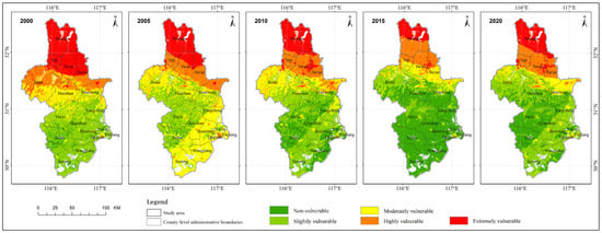
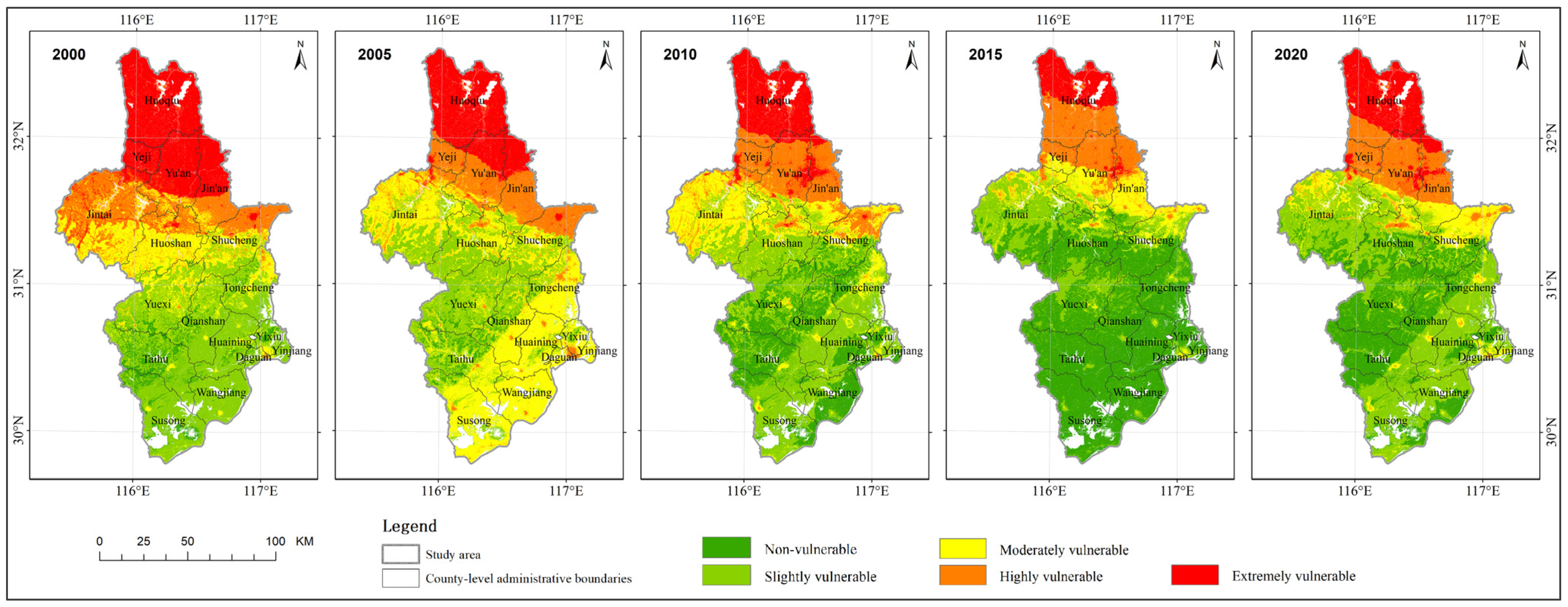
Figure 4 shows the spatial distribution of the five-period EVI classes, and Table 2 reports their area proportions. Across the 14-indicator EVI results, ecological vulnerability generally decreased, although the temporal trajectory fluctuated among periods. The combined proportion of non-vulnerable and slightly vulnerable areas increased from 40.62% in 2000 to 64.27% in 2020, whereas highly and extremely vulnerable areas decreased from 38.98% to 23.29%. The proportion of non-vulnerable and slightly vulnerable areas reached 70.03% in 2015, the highest value among the five periods.

Figure 4. Spatial distribution of ecological vulnerability from 2000 to 2020. The maps use a unified natural-break classification of five-period EVI rasters on the common 30 m reference grid.

Table 2. Area proportions of the 14-indicator EVI classes.

Year	Non-Vulnerable	Slightly Vulnerable	Moderately Vulnerable	Highly Vulnerable	Extremely Vulnerable	Highly + Extremely Vulnerable
2000	6.11%	34.51%	20.40%	15.91%	23.07%	38.98%
2005	2.47%	26.35%	41.11%	14.62%	15.45%	30.07%
2010	19.27%	34.98%	19.06%	14.08%	12.61%	26.69%
2015	49.78%	20.25%	11.40%	12.52%	6.05%	18.57%
2020	25.82%	38.45%	12.44%	12.00%	11.29%	23.29%

Using the final unified-Jenks EVI class rasters, we sampled 50,000 valid pixels common to all five periods with a fixed random seed for a paired non-parametric test. Mean ordinal class scores were 5.29, 5.27, 4.29, 3.08, and 3.88 for 2000, 2005, 2010, 2015, and 2020, respectively. The Friedman test indicated a significant distributional difference among the five periods (statistic = 109694.77, p < 0.001), and the paired Wilcoxon test confirmed a significant change between 2000 and 2020 (statistic = 7531441.00, p < 0.001). These tests support an overall downward shift in vulnerability classes while also confirming a partial rebound in 2020. Because nearby pixels are spatially autocorrelated, the p-values are interpreted as evidence of a distributional shift rather than as independent-pixel estimates of model accuracy.

Spatially, non-vulnerable and slightly vulnerable areas were mainly distributed in mountainous and hilly areas with relatively high vegetation cover and stable ecosystem structure. Highly and extremely vulnerable areas were more common in the northern part of the study area, selected urban fringes, agricultural concentration areas, and areas with a simpler ecosystem structure. In 2020, highly and extremely vulnerable areas still accounted for 23.29%, indicating that overall improvement did not eliminate local sensitivity.

Across the temporal sequence, highly and extremely vulnerable areas together approached two-fifths of the study area in 2000, and both the EVI mean and 90th percentile were highest among the five periods, indicating relatively strong climatic-background and ecological-structure pressure in the early period. The marked increase in non-vulnerable and slightly vulnerable areas in 2015 may reflect vegetation recovery, ecological-protection investment, and local improvement in land-use structure. The rebound of highly and extremely vulnerable areas in 2020 relative to 2015 suggests that ecological improvement can be stage-specific and locally reversible, underscoring the need for continuous monitoring to maintain management effectiveness.

3.2. Changes in Soil-Erosion Intensity

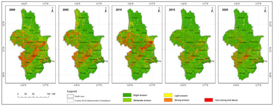
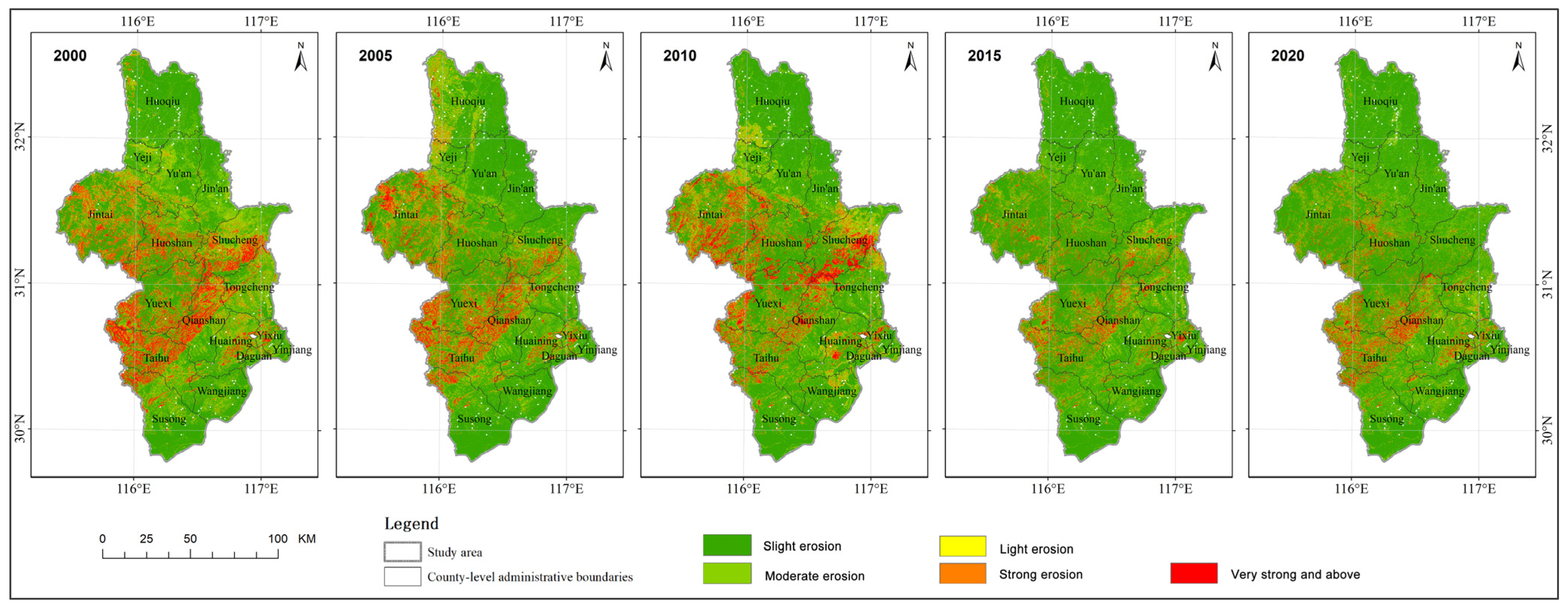
Figure 5 shows the spatial distribution of soil-erosion intensity, and Table 3 reports the class proportions. Slight and light erosion dominated the study area, whereas moderate-or-above erosion was mainly distributed on slopes, in gullies, and in hilly agricultural areas. The proportion of moderate-or-above erosion was 25.20% in 2000, decreased to 20.45% in 2005, increased slightly to 21.91% in 2010, and then declined to 12.50% and 13.56% in 2015 and 2020, respectively. Because RUSLE provides model-based estimates, the P factor was treated as a land-use proxy for support practice. In the absence of independent sediment observations, the results are interpreted as relative regional erosion pressure and should be further tested with field or watershed evidence.

Figure 5. Spatial distribution of soil-erosion intensity from 2000 to 2020. The maps are derived from the revised RUSLE implementation with DEM-based terrain factors, an FVC-based cover-management factor, and the common 30 m reference grid.

Table 3. Area proportions of soil-erosion classes.

Year	Slight Erosion	Light Erosion	Moderate Erosion	Strong Erosion	Very Strong-and-Above	Moderate-or-Above
2000	55.97%	18.83%	7.73%	5.00%	12.47%	25.20%
2005	63.99%	15.56%	6.76%	4.29%	9.40%	20.45%
2010	63.18%	14.90%	6.67%	4.16%	11.08%	21.91%
2015	74.13%	13.36%	4.81%	2.74%	4.95%	12.50%
2020	72.85%	13.58%	5.03%	2.92%	5.62%	13.56%

In 2020, slight and light erosion together accounted for 86.44%, whereas moderate, strong, and very strong-and-above erosion accounted for 13.56%. Strong and very strong-and-above erosion still occurred in sloping and hilly areas, indicating that soil and water conservation measures remain necessary in these locations.

The soil-erosion classes fluctuated across periods, with relatively higher moderate-or-above erosion in 2000 and 2010 and lower values after 2015. This pattern may reflect the combined influence of interannual rainfall erosivity, slope-cover conditions, and local land-use practices. Even when composite EVI decreases, areas affected by slope or gully erosion may still require separate management.

Table 4 reports descriptive statistics for the annual erosion modulus and provides an additional scale-free check of the class results. The mean modulus was 34.76, 27.96, 38.67, 15.05, and 16.80 t ha⁻¹ yr⁻¹ for 2000, 2005, 2010, 2015, and 2020, respectively. The corresponding medians were 2.11, 0.47, 0.00, 0.00, and 0.00 t ha⁻¹ yr⁻¹, while the 95th percentiles were 180.28, 140.47, 175.27, 75.16, and 85.75 t ha⁻¹ yr⁻¹. The large mean–median difference reflects the right-skewed distribution of the erosion modulus, in which localized high-value pixels contribute strongly to the mean. Both class proportions and distributional statistics are therefore reported.

Table 4. Descriptive statistics of the annual revised RUSLE soil-erosion modulus.

Year	Valid Pixels	Mean	Standard Deviation	Median	95th Percentile
2000	31,383,772	34.76	92.57	2.11	180.28
2005	31,369,852	27.96	125.15	0.47	140.47
2010	31,361,137	38.67	167.96	0.00	175.27
2015	31,349,540	15.05	66.09	0.00	75.16
2020	31,327,842	16.80	70.89	0.00	85.75

Note: Mean, standard deviation, median, and $P_{95}$ are reported in t ha⁻¹ yr⁻¹. The median and percentile values are calculated from the revised modulus rasters; the distribution is strongly right-skewed.

3.3. Coupled Pressure Relationship Between EVI and Soil-Erosion Classes

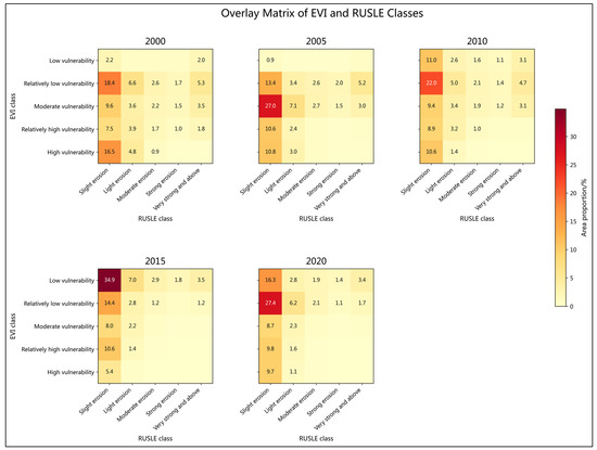
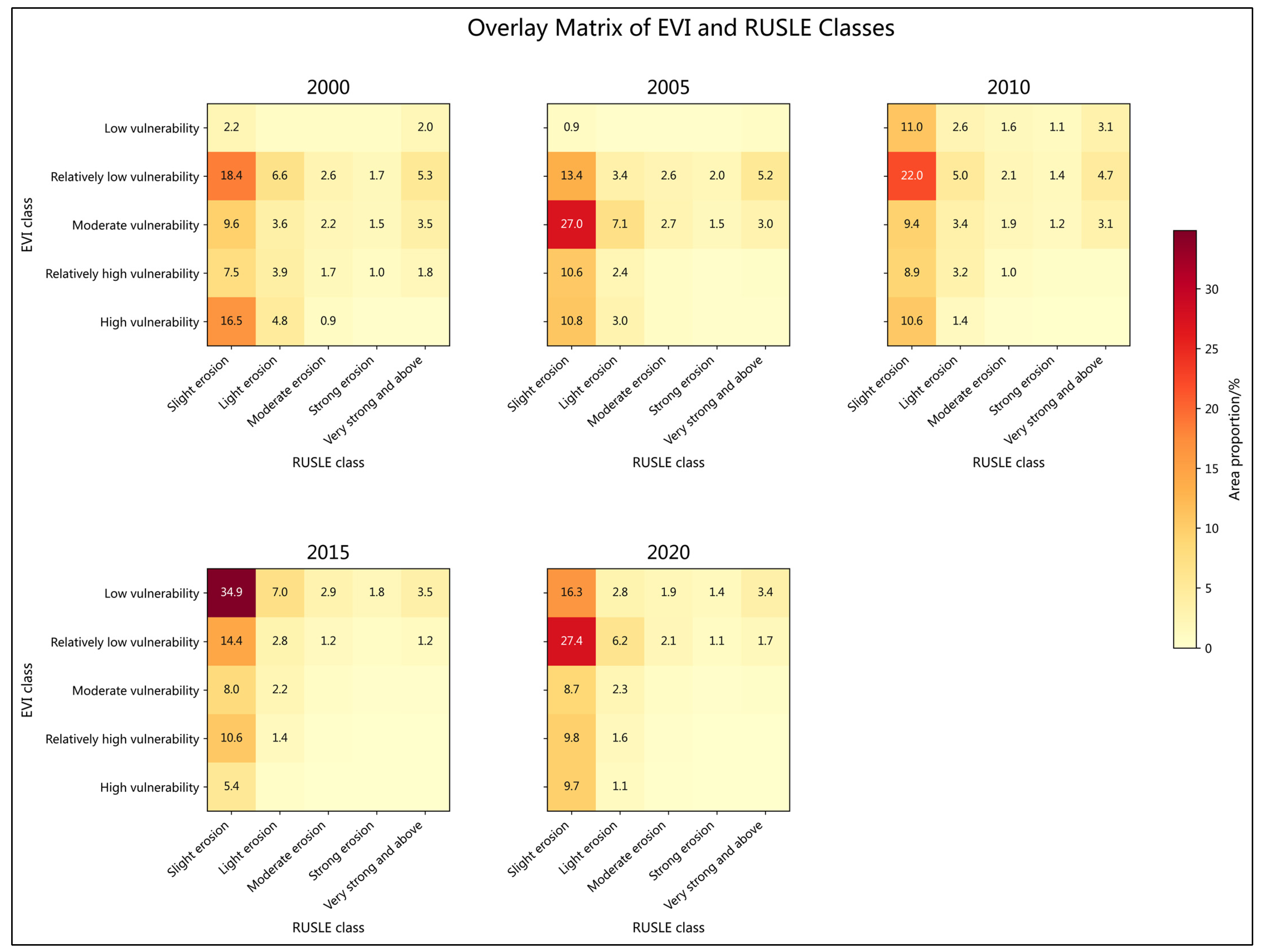
Figure 6 presents the five-period EVI–RUSLE overlay matrices. Spearman’s rho between EVI and revised soil-erosion classes was −0.228 in 2000, −0.253 in 2005, −0.175 in 2010, −0.158 in 2015, and −0.220 in 2020. Cramér’s V was 0.151, 0.147, 0.130, 0.091, and 0.131, respectively. All five years showed negative associations, indicating that the two dimensions did not simply increase together but instead represented different ecological processes and management pressures.

Figure 6. Two-row overlay matrices of EVI and RUSLE classes from 2000 to 2020. Each panel shows the cross-classification of the two ordinal layers for one selected period.

The five-period cross-matrices show that a considerable proportion of extremely vulnerable EVI areas corresponded to slight or light erosion, while moderate-or-above erosion also occurred widely in non-vulnerable, slightly vulnerable, and moderately vulnerable EVI areas. This structure was observed in multiple years, indicating that high ecological vulnerability is not necessarily equivalent to high soil erosion, and that high soil erosion does not necessarily indicate the most severe composite ecological condition.

This cross-year negative association has a clear geographic meaning. In the northern study area, highly vulnerable EVI zones were strongly affected by climatic background, ecosystem type, or construction pressure, but not all these areas exhibited strong erosion. In some western and central sloping farmland or hilly areas, EVI was not at the highest level, but soil-erosion pressure was high. Subsequent management zoning therefore needed to combine the two-dimensional pressure matrix, five-period annual-zone frequencies, CPI, IMDI, and the 2020 status rather than rely on a single year or indicator.

3.4. EVI–RUSLE Pressure-Based Management Zoning

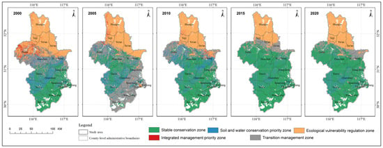
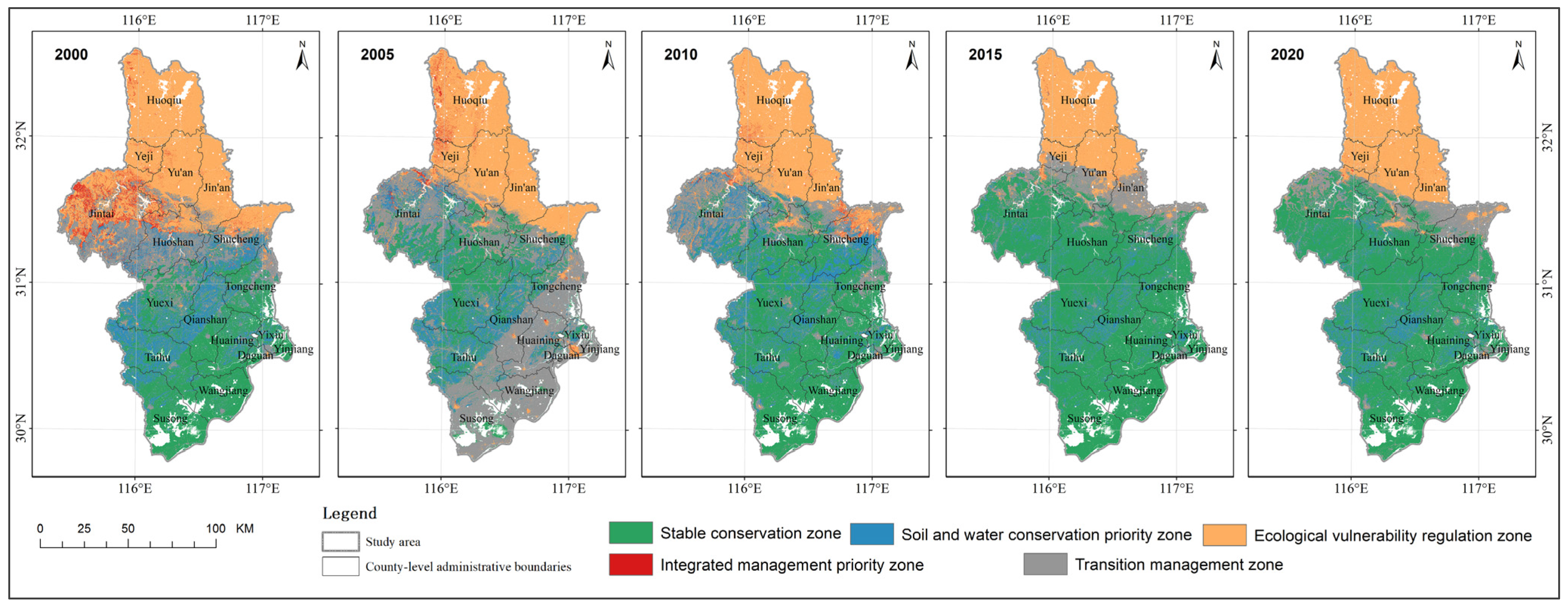
Annual EVI–RUSLE pressure zoning is mapped in Figure 7 and summarized in Table 5. Each of the years 2000, 2005, 2010, 2015, and 2020 were divided into stable conservation, soil and water conservation priority, ecological vulnerability regulation, integrated management priority, and transition management zones. Under the explicit matrix rules, integrated management priority zones accounted for 3.50%, 1.54%, 1.13%, 0.22%, and 0.33%, respectively. Soil and water conservation priority zones accounted for 14.64%, 12.65%, 14.68%, 7.73%, and 8.51%, respectively, whereas stable conservation zones increased from 27.89% in 2000 to 52.73% in 2020.

Figure 7. Annual EVI–RUSLE pressure management zoning from 2000 to 2020. The zones are derived from the explicit two-dimensional pressure matrix and the RUSLE-derived classes.

Table 5. Area statistics of annual EVI–RUSLE pressure management zones from 2000 to 2020.

Year	Stable Conservation Zone	Soil and Water Conservation Priority Zone	Ecological Vulnerability Regulation Zone	Integrated Management Priority Zone	Transition Management Zone
2000	7505.44 (27.89%)	3941.39 (14.64%)	9486.28 (35.25%)	942.30 (3.50%)	5038.16 (18.72%)
2005	4826.12 (17.93%)	3405.05 (12.65%)	7604.85 (28.26%)	414.71 (1.54%)	10,658.24 (39.61%)
2010	10,880.04 (40.45%)	3948.50 (14.68%)	6807.40 (25.31%)	302.77 (1.13%)	4957.04 (18.43%)
2015	15,866.24 (59.03%)	2079.05 (7.73%)	4863.90 (18.09%)	60.01 (0.22%)	4010.68 (14.92%)
2020	14,170.26 (52.73%)	2288.19 (8.51%)	6101.40 (22.70%)	89.57 (0.33%)	4223.47 (15.72%)

Note: Values are areas in km², with percentages of the valid study area in parentheses.

The annual maps also show a clear change in management composition. Stable conservation expanded as EVI and erosion pressures weakened in many pixels after 2010, whereas soil and water conservation priority remained concentrated in sloping and hilly areas. Ecological vulnerability regulation occupied areas where EVI remained relatively high but erosion was not simultaneously high. The integrated management priority zone was spatially localized in mountainous, hilly, and mountain–hill–plain transition areas and declined from 3.50% in 2000 to 0.33% in 2020, with a small rebound or fluctuation in years affected by higher pressure. These complementary annual zones provide the temporal evidence used to construct the five-period IMDI zoning.

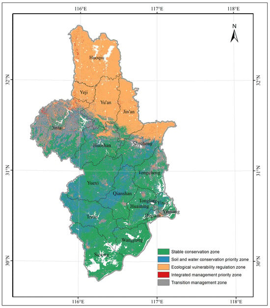
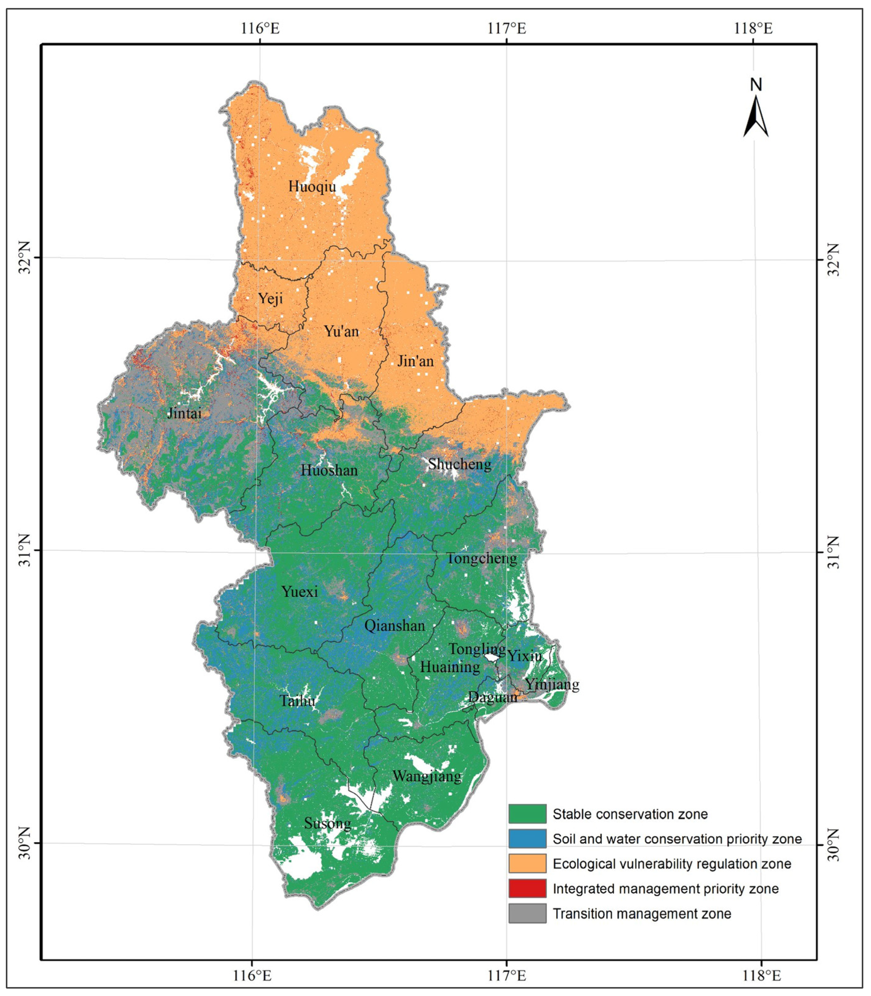
Comprehensive management zoning further integrated annual status, CPI persistence, and the current 2020 pattern through IMDI. Stable conservation zones accounted for 40.19%, mainly corresponding to areas with favorable current ecological status and high stability across the five periods. Soil and water conservation priority zones accounted for 13.73%, reflecting areas with prominent multi-year or current erosion pressure. Ecological vulnerability regulation zones accounted for 27.94%, mainly indicating areas with persistently high ecological vulnerability where erosion pressure was not the primary constraint.

Integrated management priority zones accounted for 1.48%. These areas belonged to the highest natural-break class of long-term IMDI and represented concentrated dual-pressure management demand; ecological conservation, soil and water conservation, and land-use control measures should therefore be coordinated. Transition management zones accounted for 16.66% and mostly included areas with variable annual status or moderate crossed combinations, where continuous monitoring and adaptive regulation are appropriate.

Spatially, integrated management priority zones were concentrated mainly along mountain–hill transition belts and on selected slopes, forming both patches and bands. After overlay with county-level administrative boundaries, this zone was not confined to a single administrative unit but appeared as fragmented concentrations within several mountainous and hilly counties, reflecting county-scale differences in ecological vulnerability and soil-erosion pressure.

Comprehensive management zoning uses valid 2020 pixels as the spatial base, considers the current spatial status of ecological vulnerability and soil-erosion pressure, and integrates five-period annual-zone frequencies, mean CPI, and long-term IMDI to identify areas with persistent management demand. This approach translates distinct management objectives—including stable conservation, soil and water conservation, ecological vulnerability regulation, and integrated management—into concrete spatial units, thereby providing a spatial basis for ecological conservation, soil and water conservation engineering, land-use control, and sustainable land management at county and watershed scales (Table 6).

Table 6. Comprehensive management zones based on IMDI and five-period data from 2000 to 2020.

Zone	Rule	Area/km2	Proportion
Stable conservation zone	2020 stable conservation and stable conservation appearing in at least three of five periods	10,801.03	40.19%
Soil and water conservation priority zone	soil-water priority appearing in at least two periods or in 2020, outside stable and integrated priority areas	3689.93	13.73%
Ecological vulnerability regulation zone	vulnerability regulation appearing in at least two periods or in 2020, outside stable, integrated, and soil-water priority areas	7507.66	27.94%
Integrated management priority zone	highest natural-break class of long-term IMDI outside stable conservation areas	396.60	1.48%
Transition management zone	remaining moderate or crossed combinations	4477.67	16.66%

Figure 8 shows the county-level administrative overlay, and Table 7 reports the corresponding county statistics. After the county-level overlay, IMDI-based integrated management priority zones showed localized county-level concentrations rather than broad continuous patches. Ranked by area, they were concentrated mainly in Jinzhai County (153.52 km², 4.12% of the county), Huoqiu County (64.27 km², 2.26%), Shucheng County (35.36 km², 1.76%), Huoshan County (35.00 km², 1.74%), and Yu’an District (34.72 km², 1.87%). Together, these county-level units accounted for 81.41% of the integrated management priority area in the study region.

Figure 8. County-level administrative overlay of IMDI-based comprehensive management zoning. The overlay uses the 30 m comprehensive-zoning raster and the county-level administrative units included in the study domain.

Table 7. Statistics of key management zones under county-level administrative overlay.

City	County-Level Unit	Valid Area/km2	Soil and Water Conservation Priority/%	Vulnerability Regulation/%	Integrated Management Priority/km2	Integrated Management Priority/%	Dominant Zone
Lu’an City	Jinzhai County	3730.31	15.85%	12.46%	153.52	4.12%	Transition management zone
Lu’an City	Huoqiu County	2848.49	0.00%	97.74%	64.27	2.26%	Ecological vulnerability regulation zone
Lu’an City	Shucheng County	2009.06	15.50%	34.00%	35.36	1.76%	Ecological vulnerability regulation zone
Lu’an City	Huoshan County	2014.53	17.82%	8.57%	35.00	1.74%	Stable conservation zone
Lu’an City	Yu’an District	1860.25	2.69%	81.37%	34.72	1.87%	Ecological vulnerability regulation zone
Lu’an City	Jin’an District	1582.87	1.06%	83.90%	19.18	1.21%	Ecological vulnerability regulation zone
Lu’an City	Yeji District	526.89	0.10%	95.15%	19.01	3.61%	Ecological vulnerability regulation zone
Anqing City	Yuexi County	2330.33	25.14%	0.50%	10.03	0.43%	Stable conservation zone
Anqing City	Tongcheng City	1418.02	11.45%	1.74%	7.42	0.52%	Stable conservation zone
Anqing City	Huaining County	1276.70	13.96%	0.30%	4.99	0.39%	Stable conservation zone
Anqing City	Qianshan City	1675.60	30.54%	0.15%	4.54	0.27%	Stable conservation zone
Anqing City	Yixiu District	346.03	21.60%	0.54%	2.43	0.70%	Stable conservation zone
Anqing City	Daguan District	145.33	14.99%	3.83%	1.92	1.32%	Stable conservation zone
Anqing City	Taihu County	1924.37	30.09%	0.03%	1.58	0.08%	Stable conservation zone
Anqing City	Susong County	1887.68	10.03%	0.20%	1.41	0.07%	Stable conservation zone
Anqing City	Yingjiang District	136.29	5.55%	3.71%	0.86	0.63%	Stable conservation zone
Anqing City	Wangjiang County	1158.41	4.31%	0.00%	0.35	0.03%	Stable conservation zone
Tongling City	Tongling Enclave	1.73	35.05%	0.00%	0.00	0.05%	Stable conservation zone

Note: Each proportion is the percentage of valid pixel area within the county-level unit; the integrated management priority area was calculated from 30 m pixels.

County-level management directions differed among zone types. Units with high within-county proportions of soil and water conservation priority zones included Qianshan City (30.54%), Taihu County (30.09%), Yuexi County (25.14%), Yixiu District (21.60%), and Huoshan County (17.82%). Units with high within-county proportions of ecological vulnerability regulation zones included Huoqiu County (97.74%), Yeji District (95.15%), Jin’an District (83.90%), Yu’an District (81.37%), and Shucheng County (34.00%). These differences show that pressure-matrix-based comprehensive zoning can represent the overall spatial pattern while also supporting county-level allocation of governance tasks.

The IMDI weight-sensitivity analysis showed that comprehensive zoning was stable at the whole-map scale, as summarized in Table 8. Across the 12 alternative scenarios, overall agreement with the baseline zoning ranged from 97.98% to 99.83%. Stable conservation remained unchanged at 40.19%, while the sensitivity ranges of soil and water conservation priority, ecological vulnerability regulation, and transition management zones were 1.62, 0.82, and 0.18 percentage points, respectively. The integrated management priority zone was the most sensitive class. When the persistence-frequency term was retained, its proportion ranged from 0.87% to 2.50%; it increased to 3.49% only in the diagnostic scenario that removed the persistence-frequency term, indicating that this term helps constrain temporary high-CPI pixels in long-term zoning.

Table 8. Sensitivity of IMDI-based comprehensive management zoning to alternative component weights.

Scenario	Weights Current/Mean/Frequency	Integrated Priority/%	Overall Agreement/%	Baseline Priority Retained/%	Jaccard/%
S0 Baseline	0.40/0.40/0.20	1.48	100.00	100.00	100.00
S1 Equal weights	0.33/0.33/0.34	1.36	99.79	88.87	86.20
S2 Current-emphasis	0.50/0.30/0.20	1.83	99.64	99.77	80.47
S3 Historical-mean-emphasis	0.30/0.50/0.20	2.09	99.38	99.57	70.26
S4 Persistence-emphasis	0.30/0.30/0.40	0.98	99.45	64.77	63.54
S5 Low-persistence	0.45/0.45/0.10	1.99	99.48	99.87	74.06
S6 Current + mean only	0.50/0.50/0.00	3.49	97.98	99.87	42.16
S7 High-current	0.60/0.30/0.10	1.90	99.50	97.56	74.31
S8 High-historical	0.30/0.60/0.10	2.50	98.94	98.73	57.86
S9 Current-persistence	0.50/0.20/0.30	0.87	99.37	58.27	57.77
S10 Historical-persistence	0.20/0.50/0.30	1.81	99.45	92.83	71.36
S11 Balanced-current	0.45/0.35/0.20	1.69	99.78	99.98	87.09
S12 Balanced-historical	0.35/0.45/0.20	1.62	99.83	99.15	89.43

Note: S0 is the baseline scenario used for the main comprehensive zoning. The three weights correspond to current CPI in 2020, five-period mean CPI, and the occurrence frequency of the annual integrated management priority zone. S6 is a diagnostic scenario in which the persistence-frequency term is removed. Jaccard is calculated for the integrated management priority zone relative to S0.

3.5. Validation and Plausibility Checks

The validation design distinguishes internal plausibility from external accuracy. For EVI, we checked the direction and role of all 14 indicators, the pooled class thresholds, the fixed combined weights, and the observed distributional changes across the five periods. For RUSLE, annual modulus statistics, slope gradients, and land-use cross-checks were used to test whether the spatial pattern was consistent with expected terrain-mediated erosion behavior. These checks support interpreting the outputs as relative regional prioritization; without field or watershed observations, they do not establish absolute accuracy.

The validation checks summarized in Table 9 supported the internal consistency of the results. In 2020, moderate-or-above erosion accounted for 1.60% of areas with slopes below 5°, compared with 24.85% in the 10–15° class, 28.38% in the 15–25° class, and 26.36% in areas at or above 25°. The higher values in the medium-to-steep slope classes confirm the expected topographic control, while the slight decline in the steepest class indicates the joint influence of vegetation cover, land use, and the P factor. The 2020 land-use cross-check gave moderate-or-above erosion proportions of 8.54% for cropland and 23.16% for forest, grassland, and shrubland, consistent with erosion pressure being concentrated on sloping terrain rather than reflecting a simple land-use-only effect.

Table 9. Internal validation and plausibility checks for EVI–RUSLE results and comprehensive zoning.

Check	Evidence	Interpretation
Terrain consistency	2020 moderate-or-above erosion: 1.60% (<5°), 24.85% (10–15°), 28.38% (15–25°), 26.36% (≥25°)	Higher erosion pressure in medium-to-steep slopes; residual variation reflects vegetation and land use.
Land-use consistency	2020 moderate-or-above erosion: 8.54% cropland; 23.16% forest/grass/shrub	Results are consistent with terrain-mediated erosion processes and cover differences.
Statistical association	Spearman’s rho = −0.158 to −0.253; Cramér’s V = 0.091 to 0.151 across five periods	EVI and RUSLE represent related but distinct ecological processes; the association is descriptive rather than causal.
Zoning robustness	Overall agreement with baseline = 97.98–99.83% across 12 alternative IMDI weight scenarios	The comprehensive zoning is robust at the whole-map scale; the small integrated-priority class is more sensitive.

Note: These are internal consistency and robustness checks. No field-plot or small-watershed sediment observations were available for independent RUSLE calibration. Because EVI is a weighted composite index rather than a regression equation, an external R-squared statistic is not applicable. Future work should use measured sediment yield, vegetation and land-use validation samples, and watershed monitoring for external accuracy assessment. The multi-resolution preprocessing and interpretation rules are summarized in Table 10.

Table 9. Internal validation and plausibility checks for EVI–RUSLE results and comprehensive zoning.

Check	Evidence	Interpretation
Terrain consistency	2020 moderate-or-above erosion: 1.60% (<5°), 24.85% (10–15°), 28.38% (15–25°), 26.36% (≥25°)	Higher erosion pressure in medium-to-steep slopes; residual variation reflects vegetation and land use.
Land-use consistency	2020 moderate-or-above erosion: 8.54% cropland; 23.16% forest/grass/shrub	Results are consistent with terrain-mediated erosion processes and cover differences.
Statistical association	Spearman’s rho = −0.158 to −0.253; Cramér’s V = 0.091 to 0.151 across five periods	EVI and RUSLE represent related but distinct ecological processes; the association is descriptive rather than causal.
Zoning robustness	Overall agreement with baseline = 97.98–99.83% across 12 alternative IMDI weight scenarios	The comprehensive zoning is robust at the whole-map scale; the small integrated-priority class is more sensitive.

Note: These are internal consistency and robustness checks. No field-plot or small-watershed sediment observations were available for independent RUSLE calibration. Because EVI is a weighted composite index rather than a regression equation, an external R-squared statistic is not applicable. Future work should use measured sediment yield, vegetation and land-use validation samples, and watershed monitoring for external accuracy assessment. The multi-resolution preprocessing and interpretation rules are summarized in Table 10.

Table 10. Multi-resolution preprocessing and interpretation rules.

Data type	Examples	Method	Interpretation
Continuous	Climate, DEM surfaces, K, NDVI, population, GDP, nighttime light	Bilinear interpolation	Smooth background field on the 30 m grid; no new fine-scale observations
Categorical	Soil, ecosystem, land use/land cover	Nearest neighbor	Original class codes preserved; no mixed categories
Derived/output	Flow accumulation, L/LS, EVI, RUSLE, CPI, IMDI	Common 30 m reference grid	Relative spatial pattern with residual source-scale uncertainty

Note: The 1 km inputs are used as background gradients after interpolation and are not interpreted as independent 30 m measurements.

Table 10. Multi-resolution preprocessing and interpretation rules.

Data type	Examples	Method	Interpretation
Continuous	Climate, DEM surfaces, K, NDVI, population, GDP, nighttime light	Bilinear interpolation	Smooth background field on the 30 m grid; no new fine-scale observations
Categorical	Soil, ecosystem, land use/land cover	Nearest neighbor	Original class codes preserved; no mixed categories
Derived/output	Flow accumulation, L/LS, EVI, RUSLE, CPI, IMDI	Common 30 m reference grid	Relative spatial pattern with residual source-scale uncertainty

Note: The 1 km inputs are used as background gradients after interpolation and are not interpreted as independent 30 m measurements.

3.6. Empirical Exceedance Probability and Recurrence Patterns

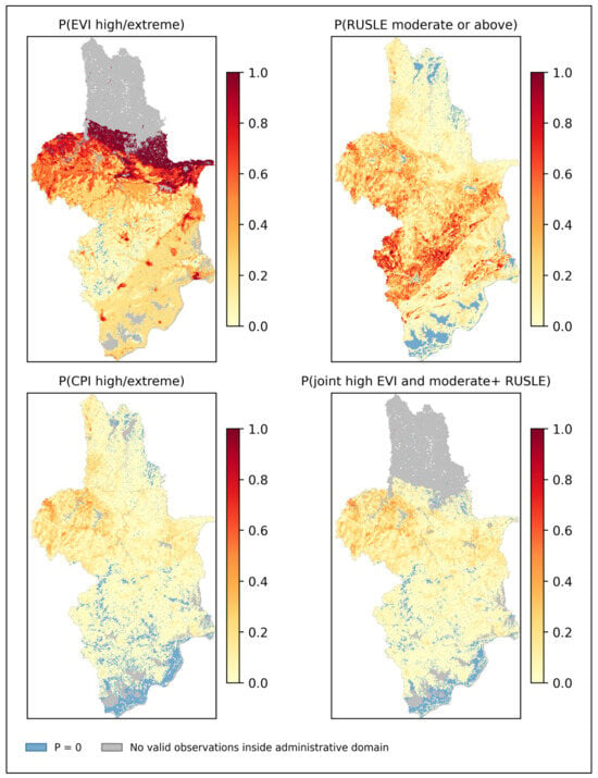
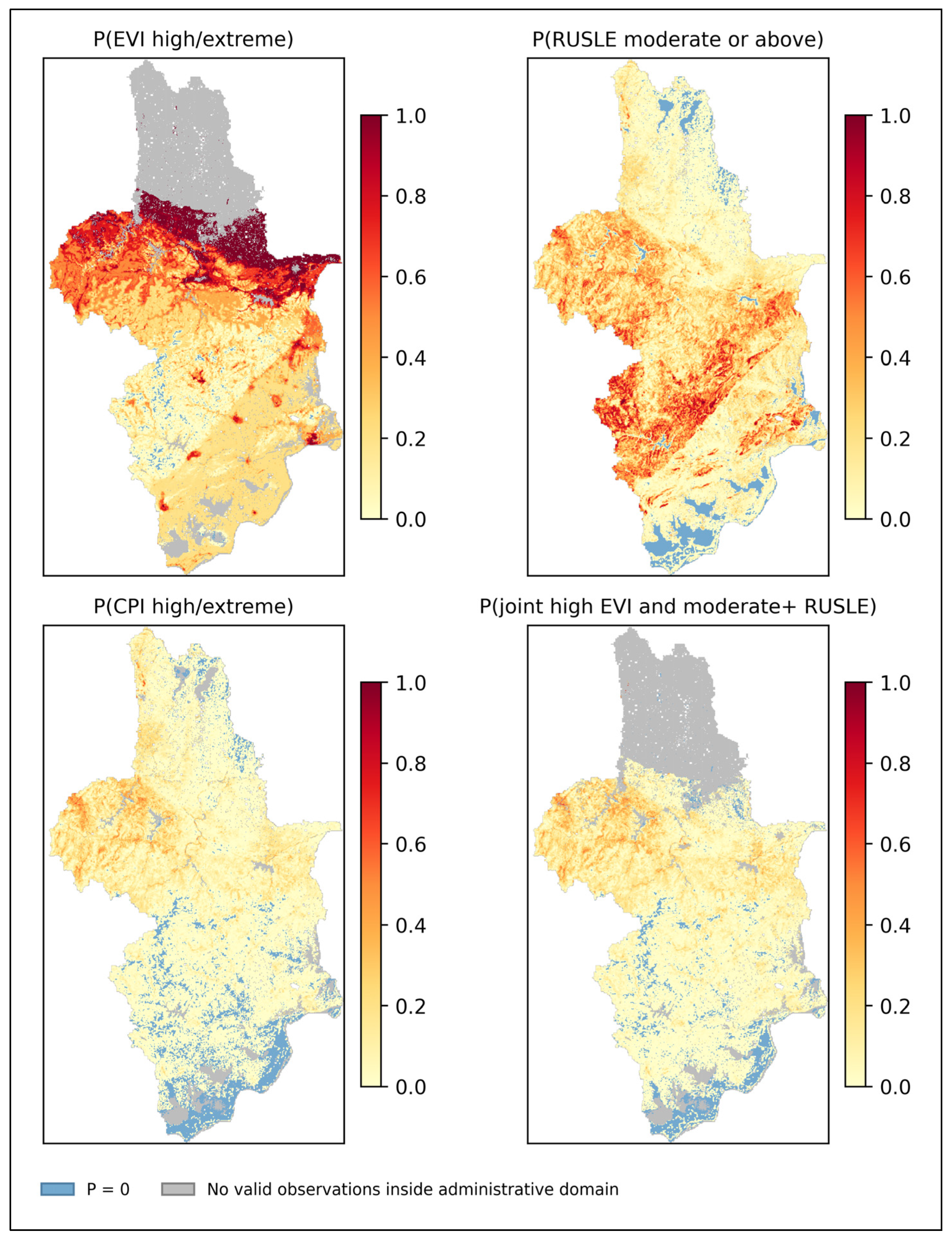
Figure 9 and Supplementary Figure S1 in the Supplementary Material File show the empirical recurrence patterns. Across the five periods, the mean empirical probability of high or extremely high EVI was 0.353; high-EVI conditions occurred at least once in 76.82% of the valid area and in all five periods in 0.20%. The corresponding mean probability for moderate-or-above RUSLE erosion was 0.187, with at least one exceedance in 39.73% of the area and recurrence in all five periods in 4.83%. High CPI occurred at least once in 18.27% of the area, whereas the joint high-EVI and moderate-or-above-RUSLE condition occurred at least once in 20.68% and in all five periods in only 0.01%. The joint exceedance pattern was therefore spatially selective, supporting the use of persistence information as a management-demand signal.

Figure 9. Empirical exceedance probabilities of EVI, RUSLE, CPI, and their joint high-pressure condition across the five selected periods. Values are recurrence frequencies over the observed periods, not long-term stochastic forecasts; areas outside the administrative domain remain white, blue indicates P = 0, and gray within the administrative domain indicates no valid observations.

4. Discussion

4.1. Management Meaning of EVI–Soil-Erosion Coupling

This study organized EVI calculation, annual EVI–RUSLE pressure zoning, and comprehensive management zoning as sequential steps. EVI derived from 14 indicators represents composite ecological vulnerability; soil-erosion intensity enters the overlay analysis as a soil and water conservation process; and CPI/IMDI describe whether the two pressures are jointly or persistently prominent within the same pixel. A global review of soil-erosion modeling shows that erosion assessment commonly relies on model-based representations, while regional process backgrounds and data conditions strongly affect interpretation [26].

The five-period results show that EVI and soil-erosion classes were moderately negatively associated, indicating that they represent different ecological processes and management dimensions. Some northern areas had high EVI but low erosion classes and may be more strongly affected by ecosystem structure, construction pressure, or climatic background. Some low-hill and sloping-farmland areas had lower EVI but higher erosion classes, making slope runoff, farming practices, and gully processes important management targets. USLE/RUSLE-type models are suitable for identifying relative erosion risk at regional scales, but their results still require interpretation alongside management scenarios and measured evidence [27].

4.2. Significance of Comprehensive Management Zoning for Sustainable Land Management

Comprehensive management zoning uses valid 2020 pixels as the spatial base and integrates five-period annual-zone frequencies, mean CPI, and long-term IMDI to identify areas with persistent management demand. Its purpose is not to assign a single intervention intensity to all areas, but to translate stable conservation, soil and water conservation, ecological vulnerability regulation, integrated management, and transition-management objectives into mappable and statistically measurable spatial units. Research on ecological-vulnerability transformation likewise emphasizes that assessment results should support the identification of regulatory pathways for spatial units [28].

Different zones correspond to different management pathways. Stable conservation zones emphasize maintaining existing ecological patterns, ecological source areas, and vegetation cover. Soil and water conservation priority zones emphasize slope-runoff regulation, sloping-farmland improvement, gully control, and small-watershed management. Ecological vulnerability regulation zones emphasize optimization of ecosystem structure, constraints on construction expansion, and ecological connectivity. Integrated management priority zones require coordinated ecological conservation, soil and water conservation, and land-use control. Transition management zones are suitable for continuous monitoring and adaptive adjustment. Research on ecological-vulnerability evolution under restoration initiatives in the Yellow River Basin indicates that zoning management should consider both long-term trends and stage-specific policy or environmental changes [29].

4.3. Spatial Governance Implications at the County Scale

The overlay with county-level administrative boundaries shows that integrated management priority zones are concentrated mainly in selected mountainous, hilly, and transition-zone counties, with Jinzhai County containing the largest area. These areas are generally characterized by pronounced terrain relief, active slope processes, and concurrent ecological vulnerability and erosion pressure, making them suitable for combined ecological restoration, soil and water conservation engineering, and land-use control. Ecological-vulnerability research in southwest mountain regions shows that mountain vulnerability can exhibit scale-dependent and nonlinear changes; county-scale decomposition therefore helps translate regional diagnosis into implementable tasks [30].

County-level management directions differ among zone types. Qianshan, Taihu, Yuexi, Yixiu, and Huoshan have stronger soil and water conservation tasks and should focus on slope-runoff regulation, sloping-farmland improvement, and gully control. Huoqiu, Yeji, Jin’an, Yu’an, and Shucheng have stronger ecological-vulnerability regulation demand and should strengthen ecosystem-structure optimization, ecological-connectivity maintenance, and constraints on construction expansion. Spatially explicit studies of mountain social–ecological systems exposed to multiple environmental hazards likewise show that integrated risk identification can be translated into differentiated management units [31]. Multi-objective ecological-restoration prioritization supports aligning regional restoration objectives with implementable spatial priorities [32]. Ecosystem-service assessment in the Dabie Mountain area further supports linking ecological management with residents’ well-being [33].

4.4. Uncertainty, Limitations, and Future Work

Several uncertainties remain and were addressed through explicit parameter documentation, internal consistency checks, and weight-sensitivity analysis. First, EVI uncertainty arises from indicator-grading direction, class thresholds, and the AHP–entropy weight structure. Unified natural breaks improve cross-period comparability but can produce unbalanced class areas and suppress year-specific extremes; the resulting classes are therefore relative ordinal groupings rather than universal ecological thresholds. The 14 indicator roles and weights are reported in Figure 3 and Appendix A, Table A5, while annual classified-input summaries and grading rules are provided in Tables S5 and S6. Following a sensitivity-analysis framework, the IMDI sensitivity analysis showed 97.98–99.83% whole-map agreement across 12 alternative-weight scenarios [34], although the small integrated management priority class was more sensitive. This class should therefore be interpreted as a concentrated management-demand signal rather than a definitive boundary for project implementation. The main residual uncertainty sources and their mitigation are summarized in Table 11.

Table 11. Main uncertainty sources, mitigation measures, and residual interpretation limits.

Uncertainty Source	Mitigation in This Study	Residual Interpretation Limit
EVI grading, weights, and natural breaks	Unified thresholds, reported 14-indicator weights, and 12 IMDI sensitivity scenarios	Priority classes remain dependent on classification and weighting choices
RUSLE L/LS, C, and P parameterization	D8 flow accumulation, capped effective slope length, FVC-based C factor, documented P mapping, and terrain/land-use checks	Relative erosion pressure is supported; absolute modulus needs field or watershed calibration
Multi-resolution alignment	Bilinear resampling for continuous variables and nearest neighbor for categorical variables on a common 30 m grid	1 km inputs provide background gradients, not independent 30 m detail
CPI/IMDI semantic and threshold choices	Explicit pressure matrix, normalized components, persistence term, and alternative-weight testing	CPI/IMDI indicate management demand based on joint pressure patterns, not causal effects
Five-period temporal sampling	Common periods and frequency-based IMDI integration	Short-lived extreme events and rapid land-use changes may be missed

Second, multi-resolution preprocessing introduces scale uncertainty. The rules summarized in Table 10 used bilinear interpolation for continuous variables and nearest-neighbor resampling for categorical variables. Bilinear interpolation preserves a smooth background gradient but cannot recover sub-grid variation in 1 km climate and socioeconomic inputs, whereas nearest-neighbor resampling preserves category identities but can retain step-like boundaries. The common 30 m grid is therefore the mapping and overlay unit, not the effective measurement resolution of every input. The results should be used for relative regional prioritization, and future work should test the zoning under multi-scale aggregation and finer-resolution observations.

Third, RUSLE uncertainty is introduced by model structure and factor parameterization. The L and LS factors were derived from DEM-based D8 flow accumulation and a capped effective slope length rather than field-measured hillslope length. The C factor used FVC-based NDVI endmembers and the reported vegetation-cover equation, whereas the P factor used land-use and conservation-practice classes; these choices may affect the absolute erosion magnitude and upper tail. RUSLE results were therefore evaluated primarily as relative regional erosion pressure, supported by slope and land-use consistency checks and by reporting both class proportions and modulus distributions. Independent sediment plots, small-watershed monitoring, engineering records, and higher-resolution terrain data are still required for external calibration. This interpretation is consistent with regional soil-erosion research emphasizing interactions between natural and human factors [35].

Fourth, CPI and IMDI were defined to identify simultaneous or persistent management demand. Their interpretation is tied to the explicit matrix rules, and the highest IMDI class remains a classification choice. The A3 alternative-weight scenarios and the A4 statistical and terrain checks provide robustness evidence, while future work should compare alternative thresholds, cost constraints, and observed management outcomes.

Fifth, the five-year interval captures long-term change but may miss short-term disturbances caused by extreme-rainfall years or rapid construction expansion. Annual remote-sensing data, land-use-change scenarios, and climate simulations could improve dynamic early-warning capacity. Finally, because no plot or watershed sediment observations were available, the present validation establishes plausibility and robustness rather than absolute accuracy. This limitation is explicit and defines a priority for subsequent field-based validation.

5. Conclusions

Using multi-source raster data for 2000, 2005, 2010, 2015, and 2020, this study integrated a sensitivity–resilience–pressure EVI based on 14 indicators with revised RUSLE soil-erosion intensity, CPI, and IMDI to establish pressure-based management zoning in the eastern Dabie Mountains.

Ecological vulnerability generally improved but remained spatially heterogeneous. The combined proportion of non-vulnerable and slightly vulnerable areas increased from 40.62% in 2000 to 64.27% in 2020, whereas highly and extremely vulnerable areas decreased from 38.98% to 23.29%. Soil-erosion pressure fluctuated among periods, with moderate-or-above erosion accounting for 13.56% in 2020. The negative EVI–RUSLE associations across all five periods indicate that composite ecological vulnerability and soil-erosion pressure represent distinct ecological processes and management demands.

The five-zone comprehensive management classification comprised stable conservation (40.19%), soil and water conservation priority (13.73%), ecological vulnerability regulation (27.94%), integrated management priority (1.48%), and transition management (16.66%). Overall agreement with the baseline zoning remained at least 97.98% across 12 alternative-weight scenarios, and Jinzhai County contained the largest integrated management priority area. The joint high-EVI and moderate-or-above erosion condition occurred at least once in 20.68% of the valid area but persisted across all five periods in only 0.01%, supporting the use of persistence information to differentiate management priorities.

The results provide a spatial basis for ecological conservation, soil and water conservation, land-use control, and county-level task allocation in mountain–hill–plain transition regions. Internal consistency checks support interpreting the maps as relative regional priorities; however, the model-based RUSLE parameterization, land-use proxy P factor, classification and weighting choices, coarse-input interpolation, and absence of independent field or sediment observations limit absolute accuracy. Field or watershed evidence should therefore be used for external validation before implementation.

References

- Turner, B.L.; Kasperson, R.E.; Matson, P.A.; McCarthy, J.J.; Corell, R.W.; Christensen, L.; Eckley, N.; Kasperson, J.X.; Luers, A.; Martello, M.L.; et al. A framework for vulnerability analysis in sustainability science. Proc. Natl. Acad. Sci. USA 2003, 100, 8074–8079. [Google Scholar] [CrossRef] [Scilit]
- Adger, W.N. Vulnerability. Glob. Environ. Change 2006, 16, 268–281. [Google Scholar] [CrossRef] [Scilit]
- Saaty, T.L. The Analytic Hierarchy Process: Planning, Priority Setting, Resource Allocation; McGraw-Hill: New York, NY, USA, 1980. [Google Scholar]
- Shannon, C.E. A mathematical theory of communication. Bell Syst. Tech. J. 1948, 27, 379–423. [Google Scholar] [CrossRef] [Scilit]
- Renard, K.G.; Foster, G.R.; Weesies, G.A.; McCool, D.K.; Yoder, D.C. Predicting Soil Erosion by Water: A Guide to Conservation Planning with the Revised Universal Soil Loss Equation (RUSLE); USDA Agriculture Handbook No. 703; United States Department of Agriculture: Washington, DC, USA, 1997.
- Borrelli, P.; Robinson, D.A.; Panagos, P.; Lugato, E.; Yang, J.E.; Alewell, C.; Wuepper, D.; Montanarella, L.; Ballabio, C. Land use and climate change impacts on global soil erosion by water (2015-2070). Proc. Natl. Acad. Sci. USA 2020, 117, 21994–22001. [Google Scholar] [CrossRef] [Scilit]
- Gong, J.; Jin, T.; Cao, E.; Wang, S.; Yan, L. Is ecological vulnerability assessment based on the VSD model and AHP-Entropy method useful for loessial forest landscape protection and adaptative management? A case study of Ziwuling Mountain Region, China. Ecol. Indic. 2022, 143, 109379. [Google Scholar] [CrossRef] [Scilit]
- Jiang, Y.; Shi, B.; Su, G.; Lu, Y.; Li, Q.; Meng, J.; Ding, Y.; Song, S.; Dai, L. Spatiotemporal analysis of ecological vulnerability in the Tibet Autonomous Region based on a pressure-state-response-management framework. Ecol. Indic. 2021, 130, 108054. [Google Scholar] [CrossRef] [Scilit]
- Wu, X.; Tang, S. Comprehensive evaluation of ecological vulnerability based on the AHP-CV method and SOM model: A case study of Badong County, China. Ecol. Indic. 2022, 137, 108758. [Google Scholar] [CrossRef] [Scilit]
- Jenks, G.F. The data model concept in statistical mapping. Int. Yearb. Cartogr. 1967, 7, 186–190. [Google Scholar]
- Wang, J.F.; Xu, C.D. Geodetector: Principle and prospective. Acta Geogr. Sin. 2017, 72, 116–134. [Google Scholar] [CrossRef]
- Ding, Y.; Chen, G. Assessment of ecological environment quality and analysis of its driving forces in the Dabie Mountain Area of Anhui Province based on the improved remote sensing ecological index. Sustainability 2025, 17, 6198. [Google Scholar] [CrossRef] [Scilit]
- Fu, B.; Liu, Y.; Meadows, M.E. Ecological restoration for sustainable development in China. Natl. Sci. Rev. 2023, 10, nwad033. [Google Scholar] [CrossRef] [Scilit]
- Wang, X.; Xu, S.; Huang, X.; Yang, C.; Li, Y. Optimization and construction of forestland ecological security pattern: A case study of the Huai River Source-Dabie Mountains in China. Forests 2025, 16, 426. [Google Scholar] [CrossRef] [Scilit]
- Tachikawa, T.; Kaku, M.; Iwasaki, A.; Gesch, D.B.; Oimoen, M.J.; Zhang, Z.; Danielson, J.J.; Krieger, T.; Curtis, B.; Haase, J.; et al. ASTER Global Digital Elevation Model Version 2: Summary of Validation Results; NASA/USGS: Sioux Falls, SD, USA, 2011.
- National Soil Survey Office. Chinese Soil, 2nd ed.; China Agriculture Press: Beijing, China, 1998. [Google Scholar]
- Yang, J.; Huang, X. The 30 m annual land cover dataset and its dynamics in China from 1990 to 2019. Earth Syst. Sci. Data 2021, 13, 3907–3925. [Google Scholar] [CrossRef] [Scilit]
- Peng, S.; Ding, Y.; Liu, W.; Li, Z. 1 km monthly temperature and precipitation dataset for China from 1901 to 2017. Earth Syst. Sci. Data 2019, 11, 1931–1946. [Google Scholar] [CrossRef] [Scilit]
- Gorelick, N.; Hancher, M.; Dixon, M.; Ilyushchenko, S.; Thau, D.; Moore, R. Google Earth Engine: Planetary-scale geospatial analysis for everyone. Remote Sens. Environ. 2017, 202, 18–27. [Google Scholar] [CrossRef] [Scilit]
- Roy, D.P.; Wulder, M.A.; Loveland, T.R.; Woodcock, C.E.; Allen, R.G.; Anderson, M.C.; Helder, D.; Irons, J.R.; Johnson, D.M.; Kennedy, R.; et al. Landsat-8: Science and product vision for terrestrial global change research. Remote Sens. Environ. 2014, 145, 154–172. [Google Scholar] [CrossRef] [Scilit]
- Ministry of Ecology and Environment of the People’s Republic of China. Technical Criterion for Ecosystem Status Evaluation (HJ 192-2015); China Environmental Science Press: Beijing, China, 2015. [Google Scholar]
- Tatem, A.J. WorldPop, open data for spatial demography. Sci. Data 2017, 4, 170004. [Google Scholar] [CrossRef] [Scilit]
- Xu, X. China’s GDP Spatial Distribution Kilometer Grid Dataset; Resource and Environment Science Data Registration and Publishing System: Beijing, China, 2017. [Google Scholar] [CrossRef]
- Li, X.; Zhou, Y.; Zhao, M.; Zhao, X. A harmonized global nighttime light dataset 1992-2018. Sci. Data 2020, 7, 168. [Google Scholar] [CrossRef] [Scilit]
- Ministry of Water Resources of the People’s Republic of China. Classification and Gradation Standard of Soil Erosion (SL 190-2007); China Water & Power Press: Beijing, China, 2008. [Google Scholar]
- Borrelli, P.; Alewell, C.; Alvarez, P.; Anache, J.A.A.; Baartman, J.; Ballabio, C.; Bezak, N.; Biddoccu, M.; Cerda, A.; Chalise, D.; et al. Soil erosion modelling: A global review and statistical analysis. Sci. Total Environ. 2021, 780, 146494. [Google Scholar] [CrossRef] [Scilit]
- Alewell, C.; Borrelli, P.; Meusburger, K.; Panagos, P. Using the USLE: Chances, challenges and limitations of soil erosion modelling. Int. Soil Water Conserv. Res. 2019, 7, 203–225. [Google Scholar] [CrossRef] [Scilit]
- Hou, K.; Tao, W.; He, D.; Li, X. A new perspective on ecological vulnerability and its transformation mechanisms. Ecosyst. Health Sustain. 2022, 8, 2115403. [Google Scholar] [CrossRef] [Scilit]
- Zhang, X.; Liu, K.; Wang, S.; Wu, T.; Li, X.; Wang, J.; Wang, D.; Zhu, H.; Tan, C.; Ji, Y. Spatiotemporal evolution of ecological vulnerability in the Yellow River Basin under ecological restoration initiatives. Ecol. Indic. 2022, 135, 108586. [Google Scholar] [CrossRef] [Scilit]
- He, S.; Nong, L.; Wang, J.; Zhong, X.; Ma, J. Revealing various change characteristics and drivers of ecological vulnerability in the mountains of southwest China. Ecol. Indic. 2024, 167, 112680. [Google Scholar] [CrossRef] [Scilit]
- Pirasteh, S.; Fang, Y.; Mafi-Gholami, D.; Abulibdeh, A.; Nouri-Kamari, A.; Khonsari, N. Enhancing vulnerability assessment through spatially explicit modeling of mountain social-ecological systems exposed to multiple environmental hazards. Sci. Total Environ. 2024, 930, 172744. [Google Scholar] [CrossRef] [Scilit]
- Zhao, Y.; Liu, S.; Liu, H.; Wang, F.; Dong, Y.; Wu, G.; Li, Y.; Wang, W.; Tran, L.-S.P.; Li, W. Multi-objective ecological restoration priority in China: Cost-benefit optimization in different ecological performance regimes based on planetary boundaries. J. Environ. Manag. 2024, 356, 120701. [Google Scholar] [CrossRef] [Scilit]
- Huang, M.; Zhang, G.; Wang, Q.; Yin, Q.; Wang, J.; Li, W.; Feng, S.; Ke, Q.; Guo, Q. Evaluation of typical ecosystem services in Dabie Mountain area and its application in improving residents’ well-being. Front. Plant Sci. 2023, 14, 1195644. [Google Scholar] [CrossRef] [Scilit]
- Pianosi, F.; Beven, K.; Freer, J.; Hall, J.W.; Rougier, J.; Stephenson, D.B.; Wagener, T. Sensitivity analysis of environmental models: A systematic review with practical workflow. Environ. Model. Softw. 2016, 79, 214–232. [Google Scholar] [CrossRef] [Scilit]
- Adetona, A.M.; Martin, W.K.; Warren, S.H.; Hanley, N.M.; Huang, D.; Yang, X.; Cai, H.; Xiao, Z.; Han, D. Identifying Human-Induced Spatial Differences of Soil Erosion Change in a Hilly Red Soil Region of Southern China. Sustainability 2019, 11, 3103. [Google Scholar] [CrossRef] [Scilit]
Disclaimer/Publisher’s Note: The statements, opinions and data contained in all publications are solely those of the individual author(s) and contributor(s) and not of MDPI and/or the editor(s). MDPI and/or the editor(s) disclaim responsibility for any injury to people or property resulting from any ideas, methods, instructions or products referred to in the content. |
© 2026 by the authors. Licensee MDPI, Basel, Switzerland. This article is an open access article distributed under the terms and conditions of the Creative Commons Attribution (CC BY) license.