


Abstract
Existing approaches for rebalancing shared autonomous vehicles (SAVs) typically employ a two-step procedure, in which the future travel demand is first predicted and then fed to rebalance decision-making process. As a result, prediction errors are accumulated and propagated to the second stage, leading to inferior rebalance performance. To tackle this problem, this work proposes a deep learning-based approach to map real-time system state to vehicle rebalance decision in one step to eliminate decoupling errors. The deep learning-based method is based on a cascaded long short-term memory (LSTM) and bidirectional gated recurrent unit (BiGRU) network. Training data set is generated by applying a mathematical rebalance model to a simulation model, which allows the emergence of congestion. Numerical experiments are performed with the taxi travel data from the Manhattan road network. Compared with the mathematical rebalance model, the proposed approach achieves better performance in terms of the average passenger waiting time, total vehicle miles traveled, total system operating cost, and congestion level. The independent LSTM model has a larger impact on congestion reduction (up to 42.4%) but leads to a large portion of unsatisfied demand, while the proposed integrated approach achieves a better trade-off between congestion alleviation and level of service. These findings provide practical management insights for SAV fleet operators devoted to formulating sustainable shared on-demand mobility systems.
1. Introduction
The advancement of autonomous driving technology has given rise to autonomous mobility-on-demand (AMoD) systems, for example, Waymo, Robotaxi, and Apollo Go. Users can book via mobile applications and enjoy autonomous rides within designated areas. As a result, shared autonomous vehicles (SAVs) are becoming a key component of urban transportation systems [1]. Recent research has shown that such services can improve urban travel efficiency at reduce costs, and they are already competitive with private vehicles and public transportation [2]. In the near future, the widespread use of shared autonomous vehicles will inevitably raise the rebalancing problem faced by traditional taxis. Specifically, AMoD service providers will have to redistribute SAVs within designated areas to adjust service availability, meet future travel demand, or optimize profits and operating costs [3,4].
However, real-time travel demand is inherently asymmetric in both time and space, and thus the spatial equilibrium of SAV fleets will be disrupted constantly, leading to severe imbalance between service supply and demand. To address this issue, the vehicle rebalance problem is formulated and solved in previous studies with a “predict-then-optimize” paradigm. Forecasting models are first used to predict future regional travel demand. The obtained travel demand is then fed to mathematical models to decide how many vehicles should be relocated between operation zones. The rebalance problem is generally formulated as mixed-integer linear programming (MILP) or fluid models [5]. However, this approach has two limitations in the dynamic urban environment. First, because the demand prediction model is trained independently to minimize statistical errors, it is blind to the following rebalance model. Consequently, prediction errors are passed and amplified at the rebalance decision-making stage, leading to suboptimal vehicle rebalance. Second, the execution of relocation decisions is also influenced by urban traffic, which is usually simplified by existing approaches because modeling the emergence of urban congestion effects mathematically is computationally highly intensive.
To fill these gaps, this paper proposes a deep learning-based rebalance model to map congestion-aware system states to rebalance decisions in real time. The neural network is built by integrating long short-term memory (LSTM) and a bidirectional gated recurrent unit (BiGRU) network. Training data is obtained by running a discrete event simulation (DES) of the AMoD system with relocation decisions calculated by solving a traditional mathematical rebalance model online. Since the DES simulation is capable of emerging congestion of the road network, the formulated deep learning network is trained with congestion-aware datasets. Once trained, the deep learning-based rebalance model can produce congestion-aware rebalance decisions, solving the error propagation problem of decoupled approaches.
The contributions of this study are as follows:
- (1)
- We propose an end-to-end surrogate paradigm that merges demand prediction and rebalance optimization into a single neural network forward pass, bypassing the problems stems from the decoupled predict-then-optimize approaches.
- (2)
- We build a congestion-aware DES model with embedded a traditional mathematical optimization model to generate offline training datasets.
- (3)
- We replace the traditional rebalance model in the DES with the trained deep learning-based method, demonstrating the performance of the proposed approach.
The remainder of the paper is organized as follows. Section 2 reviews related work. Section 3 formally states the congestion-aware SAV rebalancing problem. Section 4 presents the overall methodology, DES, and feature selection. Section 5 presents the experimental results. Section 6 discusses the operational trade-offs and practical implications obtained. Section 7 concludes this work with future directions.
2. Literature Review
This section reviews related works in the following research fields: the evolution of rebalancing methods and the role of simulation in evaluating rebalancing strategies.
2.1. Rebalancing Methods of Shared Autonomous Vehicles
Most existing AMoD systems employ reactive dispatch strategies, which can be categorized into steady-state and real-time optimization methods. Steady-state approaches assume that the transportation road network is always in equilibrium. For instance, Pavone et al. [5] used fluid models to balance vehicle distributions across zones, while Smith et al. [6] extended this model by incorporating routing and dispatcher constraints. Zhang and Pavone [7] utilized queuing theory to formulate the rebalancing problem as a linear programming to regulate vehicle queue length. For real-time operations, reactive strategies like the MILP-based heuristic proposed by Kek et al. [8] adapt dynamically to incoming requests but remain computationally demanding. While greedy algorithms (e.g., assigning the nearest idle vehicle to a travel request [9]) are computationally simple and short-sighted, they lead to inevitable spatial imbalances and empty vehicle accumulation under asymmetric demand.
To overcome these reactive limitations, proactive dispatch strategies pre-emptively relocate idle vehicles to anticipated high-demand zones. Early proactive methods rely on receding horizon control or model predictive control [10], which are theoretically sound but highly sensitive to prediction errors.
In recent years, the decoupled predict-then-decide framework has gained prominence. In this paradigm, forecasting and decision-making are executed sequentially. For instance, Iglesias et al. [11] utilized an LSTM network to first predict origin–destination demand matrices, and then solved a real-time model predictive control (MPC) problem to relocate vehicles. In recent years, deep reinforcement learning (DRL) and multi-agent reinforcement learning (MARL) have emerged as powerful paradigms to solve proactive fleet rebalancing. For instance, Wen et al. [12] applied deep Q-networks to optimize inter-zone vehicle relocation based on high-dimensional state representations. Furthermore, multi-agent reinforcement learning frameworks have been developed to coordinate fleet actions under dynamic environment states. Despite their progress, these model-free reinforcement learning approaches can be computationally intensive to train online and heavily depend on custom reward functions that are difficult to calibrate.
Despite their progress, these decoupled predict-then-optimize frameworks suffer from two limitations:
- (1)
- Propagation of travel demand prediction error: The travel demand prediction and rebalancing optimization problems are isolated, which leads to the propagation of forecasting noise and prediction errors from the first stage to the subsequent optimization stage, distorting the final rebalancing decisions.
- (2)
- Neglect of real-world congestion effects: Existing approaches typically assume simplified, static inter-zone travel times and fail to account for the random traffic congestion that emerges randomly in real-world urban road networks. In practical applications, ignoring such congestion dynamics can lead to delayed or unfeasible relocation plans.
These gaps highlight the need for a unified, congestion-aware framework that can bypass the decoupled sequence entirely.
2.2. Simulation Models in SAV Dispatch
Simulation platforms are used to evaluate and validate AMoD operational strategies under dynamic urban conditions. Early studies, such as those by Fagnant and Kockelman [13], utilized agent-based simulations to analyze the impact of fleet size on service levels [14,15]. To capture highly complex operational interactions in SAV networks, agent-based discrete event simulations (DES) have been increasingly deployed [16,17,18], providing a robust testing bed for fleet performance evaluation under congestion effects.
However, computational efficiency remains a major bottleneck in large-scale urban simulations. Time-driven simulation platforms, such as MATSim [19], require continuous, system-wide updates of all entities at fixed time steps, leading to prohibitive computational costs in metropolitan scenarios. In DES models, system state is updated only when discrete events occur, which leads to reduced computation budgets. Leveraging this advantage, Yang et al. [20] and Yang et al. [21] utilised DES to optimize electric fleet size and charging infrastructure sizing, while incorporating endogenous congestion and limited link space [21,22]. Furthermore, simulation-based design approaches have demonstrated significant success in parameters optimization (such as transit headways) under stochastic environments [23], establishing the validity of using simulations to guide transit system operation. To validate and verify these simulated processes, robust validation frameworks have been proposed [24].
Simulation models have also been applied to investigate various urban mobility scenarios. Bischoff and Maciejewski [25] simulated city-wide replacements of private cars with autonomous taxis in Berlin, showing that vehicle sharing rates correlate positively with urban density. Levin et al. [26] developed a bi-level optimization framework integrating dynamic network loading and real-time ride-sharing, although their reliance on static historical demand limits their method’s adaptability to unexpected network fluctuations. Additionally, dynamic planning has been applied to joint fleet sizing and charging facility layouts under restricted power grid capacities [27], though these models often assume simplified traffic flow dynamics.
3. Problem Statement
We consider a single AMoD system providing on-demand mobility service over a zoned urban road network. The operation area is partitioned into a set of discrete zones denoted by S, indexed by . The planning horizon is discretized into uniform decision time steps indexed by , where each time step has a predefined time span of minutes. At each decision interval t, the operator of the AMoD system is responsible for making rebalancing decisions to redistribute SAVs to meet future travel demands.
The state of each operation zone during any time step t is characterized by the following parameters:
- : The number of travel requests originating from zone i during the decision interval t.
- : The number of empty SAVs that can be relocated in zone i during decision interval t.
- : The number of SAVs currently traveling toward zone i (including passenger-carrying and already relocated vehicles) that will arrive in the next decision interval.
At each decision time point t, the task of the AMoD operator is to determine how many SAVs () should be relocated from zone to for all pairs. Conceptually, the rebalancing decision aims to minimize a system-level operational cost function , which represents a non-linear combination of passenger wait times, unsatisfied demand penalties, and empty vehicle vehicle kilometers traveled (VKT):
where is the average passenger wait time in zone i; is the number of unsatisfied passengers; is the predicted number of travel requests originating from zone i during the next decision interval; is the vehicle kilometers traveled during relocation; and are the cost coefficients.
In conventional proactive operations, solving the vehicle rebalancing problem typically relies on a decoupled, two-stage “predict-then-optimize” (or predict-then-decide) framework. In this decoupled setup, future passenger demand and system states are predicted independently in the first stage, and then treated as deterministic inputs for mathematical optimization in the second stage. However, this decoupled setup completely isolates prediction from decision-making. Because the forecasting model is trained under generic statistical metrics (e.g., mean squared error) without considering the downstream optimization objective, it neglects prediction uncertainty and accuracy during the decision-making phase. Consequently, the inevitable forecasting errors from the first stage propagate non-linearly and amplify during the subsequent optimization stage, resulting in highly sub-optimal or even practically infeasible rebalancing decisions.
To fundamentally eliminate this error propagation and bridge the gap between travel demand forecasting and rebalancing decision-making, we reformulate the rebalancing problem as an end-to-end surrogate mapping problem. Instead of executing prediction and optimization in isolated sequential stages, we learn a unified surrogate function F parameterized by neural network weights that directly maps the historical AMoD system states to the relocation decisions :
where is the historical multi-variate feature matrix spanning a sliding window of length w.
4. Methodology
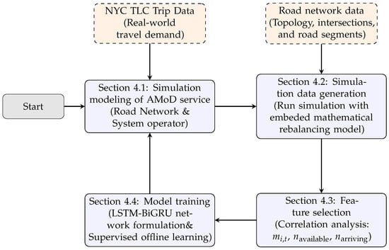
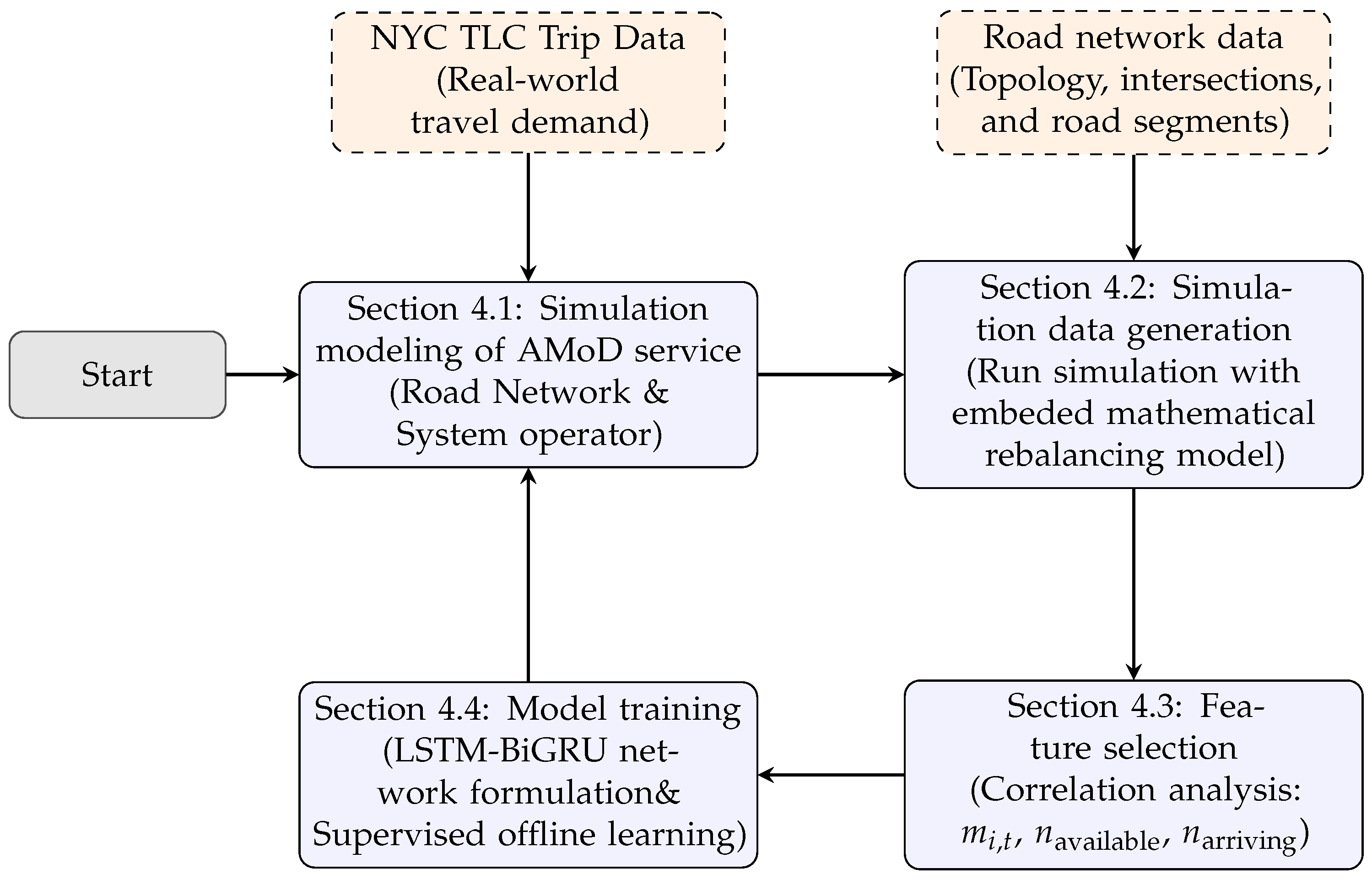
This section presents the proposed methodology to formulate and train the deep learning-based surrogate rebalancing model in four steps, as shown in Figure 1.
Figure 1.
Flowchart of the proposed deep learning-based surrogate framework.
- (1)
- Simulation modeling of AMoD service systems (Section 4.1): Based on discrete event simulation theory, we build a simulation model of AMoD service systems, which incorporates intersections, congestion-aware streets, SAVs, travel request generator, and the rebalancing module for SAV rebalancing (i.e., the operator).
- (2)
- Simulation data generation (Section 4.2): We select a traditional mathematical rebalancing model to generate SAV rebalancing decisions in the simulation model (representing the operator). With predefined supply-side parameters (e.g., fleet size) and the historical NYC TLC trip dataset [28], the simulation model is run multiple times to generate simulation datasets for feature selection.
- (3)
- Feature Selection (Section 4.3): Raw simulation data are aggregated over hexagonal zones. Spearman rank correlation analysis is performed to statistically validate the selected core state features: regional demand, available vehicles, and en-route vehicles.
- (4)
- LSTM-BiGRU network training (Section 4.4): The filtered features are scaled and processed via a sliding window. The cascaded LSTM-BiGRU network processes these temporal patterns to output the relocation decision matrix Y directly in a single forward pass.
4.1. Simulation Modeling of AMoD Service Systems
To generate training data and evaluate the performance of the proposed deep learning-based framework, we construct a congestion-aware DES model as the operational environment. In the simulation, the road network is discretized into directed streets and intersections. Travel requests are generated and picked up at any point of the directed streets. The complex vehicle traversal and rebalancing processes are modeled through discrete events. These events are classified into three primary categories to represent street congestion, passenger interactions with SAVs, and fleet management:
- Traffic and traversal events: These manage vehicle movements and queue transitions along the directed links, including Link Update, Speed Update, Entry, Completion, Exit, and Entry Update events, allowing congestion to emerge dynamically.
- Passenger interaction events: These govern demand generation and trip execution, including Passenger Arrival, Pickup, Drop-off, as well as Halfway Entry and Halfway Exit events.
- Fleet allocation events: These coordinate vehicle state transitions under operator commands, representing SAV rebalancing.
The underlying execution process of the DES model rests upon the interaction of three core architectural components:
- Object modules: These represent the fundamental entities of the AMoD network, including streets, intersections/nodes, passengers, SAVs, and the central operator. Each object encapsulates specific internal state variables and custom logic definitions to govern its response to operational events, enabling realistic representations of dynamic fleet interactions.
- Future event list (FEL): The FEL serves as the scheduler of the simulation, maintaining all generated events in a queue sorted chronologically by their execution timestamps. The simulation progresses by sequentially processing events from the head of the FEL, ensuring strict chronological and system consistency.
- Simulation clock: Rather than advancing in uniform, discrete intervals, the simulation clock tracks time asynchronously, hopping directly to the execution timestamp of the current event being processed.
At each rebalancing interval, the operator module of the DES engine collect system state data and make rebalancing decision according to predefined methods.
4.2. Simulation Data Generation
In this subsection, we incorporate the following mathematical model into the operator module of the simulation model in the last subsection to generate training data for the deep learning model . The selected rebalancing model is the feedforward fluidic optimal rebalancing policy (FF) proposed by Pavone et al. [5]:
Under this paradigm, the SAV movements on the road network are modeled as a continuous fluid system. The core ideal of this policy is to balance the vehicle flows across the operating zones to maintain a steady-state spatial equilibrium.
The mathematical model requires the following input parameters extracted from the simulation model.
- : The travel time required for an SAV to travel from zone i to zone j.
- : The average passenger arrival rate (demand intensity) originating from zone i.
- : The transition probability of passengers traveling from zone i to j, representing the spatial destination distribution of local demand.
- : The pre-defined rebalancing time step interval.
- : The decision variable representing the optimal steady-state rebalancing flow rate of empty vehicles rebalanced from zone i to zone j.
The feedforward fluidic rebalancing policy is formulated as a linear programming model as follows. The objective (3) is to minimize the total vehicle travel time of rebalancing flows across the directed graph. The mathematical optimization model is formulated as follows:
Equation (4) represents the flow balance constraint at each vertex . The left-hand side calculates the net rebalancing flow out of zone i, while the right-hand side represents the net loss of vehicles in that zone due to passenger trips (defined as the difference between the local passenger arrival rate and the incoming passengers arriving from all other zones ). Equation (5) is the non-negativity constraint restricting the rebalancing rates to be non-negative. By solving this linear program, the optimal rebalancing rates are obtained and integrated continuously over . When the integrated value exceeds one, a single SAV is dispatched to execute the relocation in the simulator.
4.3. Feature Selection
In this subsection, we select the features used in the deep learning network. In the SAV dispatch volume prediction scenario, numerous factors influence vehicle relocation, such as passenger demand, vehicle distribution, road congestion, and temporal characteristics. Through an in-depth qualitative screening of SAV operational dynamics, followed by a quantitative correlation analysis, we select three core features as inputs for the LSTM-BiGRU model: regional demand, en-route vehicles, and parked available vehicles. Below, we detail the definitions and logical relationships of these core features, and quantitatively validate their selection using Spearman’s rank correlation coefficient.
- Regional demand (): Represents the travel request volume originating within zone i during interval t, directly driving vehicle inflows and outflows under supply–demand imbalances.
- En-route vehicles (): The total number of incoming vehicles (including empty, pickup, and occupied trips), reflecting pre-allocated capacity and local real-time operational constraints.
- Parked vehicles (): The volume of idle, unassigned vehicles immediately available in zone i, serving as the direct resource pool for relocation decisions.
To evaluate the statistical significance and informational redundancy of these features, we perform a Spearman rank correlation analysis on the simulated dataset, using total dispatch volume as the dependent variable. The resulting correlation matrix is presented in Table 1.
Table 1.
Spearman rank correlation of candidate parameters.
The statistical results in Table 1 validate our feature selection. The total dispatch volume exhibits strong negative correlations with both regional demand () and en-route vehicles (), alongside a statistically significant weak positive correlation with parked vehicles (). Furthermore, the strong positive correlation between regional demand and en-route vehicles () reflects transit dynamics—rising passenger demand naturally triggers vehicle dispatches—representing a complementary spatiotemporal linkage rather than informational redundancy. Conversely, parked available vehicles show negligible correlation with both demand () and en-route vehicles (), proving that idle resources are linearly independent of demand-driven states and capture a distinct, non-redundant dimension of the fleet distribution.
By now, the surrogate model directly integrates demand forecasting and decision-making into a single forward pass.
4.4. LSTM-BiGRU Network Training and Deployment
To capture the nonlinear temporal dependencies and complex regional interactions of dispatch demands within simulated dynamics, we develop a deep learning-based method, which integrates LSTM and BiGRU networks. This section details the structure of the neural network and its training procedure.
4.4.1. Input Layer and Data Preprocessing
The input layer establishes multivariate historical time-series sequences derived from the discrete event simulation model. For each operating zone, three core spatiotemporal state features are extracted: regional demand (), en-route vehicles (), and parked available vehicles ().
Following the temporal data preprocessing steps outlined at the beginning of this section, the travel demand is aggregated at min intervals to construct standardized input sequences. To eliminate dimensional scaling discrepancies among demands and vehicle counts, thereby stabilizing gradient descent and accelerating convergence, a Min–Max normalization is applied to all input features before model training:
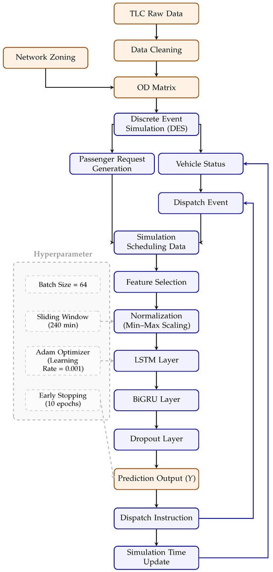
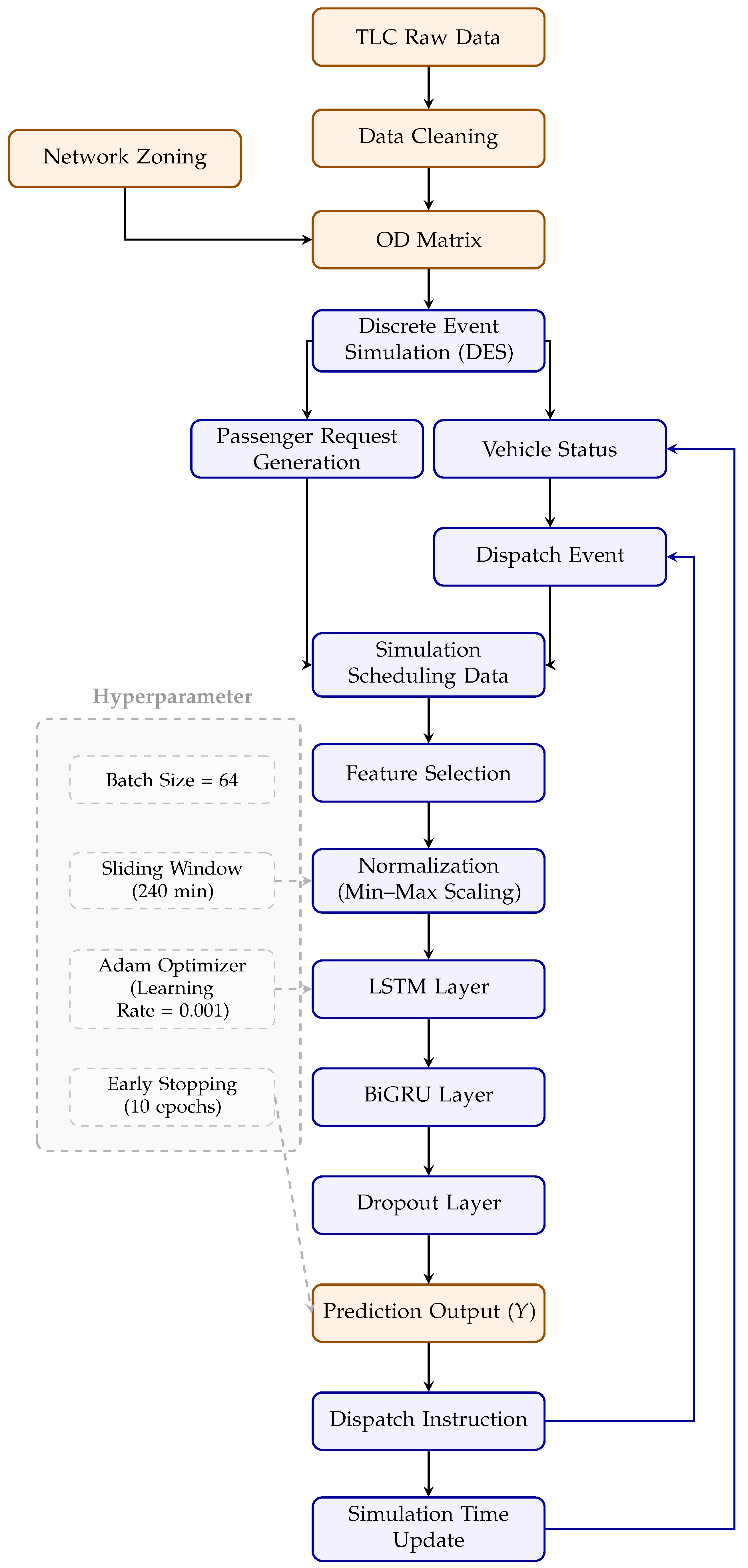
where x represents the raw feature value; and are the minimum and maximum values of the feature across the dataset; and is the normalized feature. The standardized spatiotemporal sequences are then structured as multivariate temporal tensors, as conceptually illustrated in Figure 2.
Figure 2.
Data flow and processing structure of the cascaded LSTM-BiGRU model.
4.4.2. Hybrid Cascade Hidden Layer
The hybrid hidden layer utilizes a two-stage cascaded architecture to perform deep spatial–temporal encoding on the input tensors.
- Stage 1:
- LSTM Layer
The first stage comprises multiple cascaded LSTM units. Through the cooperative control of the forget gate, input gate, output gate, and cell memory state, the LSTM cells successfully model the long-range temporal trends and feature dependencies in the dispatch data [29], effectively mitigating the gradient vanishing issues of standard recurrent neural networks. At each time step t, for an input vector , the LSTM update process is formulated as follows:
where , , and represent the forget, input, and output gate vectors, respectively; and are the cell state and candidate cell state vectors, respectively; , , and () denote the learnable weights and biases; is the Sigmoid activation function; and ⊙ represents the Hadamard product.
- Stage 2:
- BiGRU Layer
The second stage consists of a bidirectional gated recurrent unit (BiGRU) layer, which processes the output sequences of the LSTM layer bidirectionally. By integrating both forward and backward temporal contexts of the historical sequence, the BiGRU layer enhances the model’s situational awareness under rapid regional fluctuations, further extracting the underlying spatial–temporal interaction features of dispatch actions among different zones [30].
The forward GRU computes forward hidden states , while the backward GRU processes the sequence in reverse to obtain backward states . For the forward path, the update process is represented as:
The final hidden representation at step t concatenates both directional sequences to synthesize global temporal contexts:
4.4.3. Output Layer and Decision Mapping
The output layer maps the combined spatiotemporal features of the last time step to the vehicle dispatch decisions across regions. The output is formulated as:
where and are the weights and biases of the fully connected output layer. The ReLU activation function is applied to ensure that the predicted relocation volume from zone i to zone j remains non-negative. This output matrix provides real-time SAV rebalancing decisions.
Although the ReLU activation function ensures non-negativity of the predicted relocation commands, the end-to-end neural network surrogate cannot mathematically guarantee strict compliance with conservation constraints (e.g., the total predicted relocation volume out of zone i exceeding its actual available parked vehicles ). To ensure absolute consistency in the system, a proportional scaling rule is implemented inside the DES environment. Specifically, if the sum of predicted relocation outflows from zone i exceeds the actual local supply, i.e., , the executed relocation volume is dynamically scaled down and integer-truncated as follows:
This proportional truncation mechanism ensures that the fleet boundary constraints are strictly satisfied at every simulation time step without interrupting the continuous sub-second inference pipeline. Simulation analysis shows that this proportional scaling correction is activated in only 4.5% of the total decision intervals (approximately 3.37 intervals out of 75 steps per simulation day), with an average excess outflow of only 1.8 vehicles per zone and an average scaling factor of 0.87. This low activation frequency confirms that the trained network has already learned the supply boundary constraints, meaning this scaling mechanism functions primarily as an online safeguard rather than a dominant, active part of the relocation policy.
4.4.4. Supervised Sliding Window and Training Strategy
To extract the cyclical patterns, fluctuations, and short-term anomalies of traffic demand, a sliding window sampling strategy is adopted to generate supervised samples. The input sequence length is set to consecutive time steps (representing a historical horizon of 240 min), which is mapped to predict the optimal relocation matrix Y for the next 20 min (). This setup aligns with the 20 min rebalancing cycle of the SAV system. Under this setup, each 25 h simulation run (containing 75 temporal intervals) is segmented into 63 supervised samples. Across the eight independent simulation runs, the total dataset size comprises 504 samples. To prevent temporal data leakage, the dataset is split strictly by simulation runs rather than individual time steps; specifically, 75% of the dataset (six simulation runs, yielding 378 samples) is allocated for training, while the remaining 25% is divided equally: one simulation run (63 samples, or 12.5% of the total dataset) is designated as the validation set to monitor training loss and trigger early stopping, and the final simulation run (63 samples, or 12.5% of the total dataset) is held out entirely as the test set for offline performance evaluation. The sliding window moves step-by-step along the time axis, generating a high-density, full-coverage dataset that spans peak, off-peak, and low-demand conditions. To improve generalization and prevent overfitting, a Dropout layer with a dropout rate of 0.2 is introduced within the hybrid architecture, which randomly deactivates a fraction of neurons during training to mitigate co-adaptation. The network is optimized using the Adam optimizer with its self-adaptive learning rate capabilities. To ensure experimental reproducibility, the random seeds for both Python (Version 3.8) and NumPy (Version 1.26.4) are fixed to 1, and the simulation’s pseudo-random number generator is initialized with a constant seed of 0. The critical training hyperparameters are configured as follows: the number of hidden units in both the LSTM and BiGRU layers is set to 64, the initial learning rate is set to 0.001, and the batch size is set to 64, balancing training stability and computational efficiency.
Additionally, an early-stopping mechanism is implemented to prevent overtraining: the validation loss is monitored during training, and if it fails to improve for 10 consecutive epochs, training is terminated, and the optimal model weights are preserved. The finalized model is then reintegrated into the DES platform to execute real-time vehicle rebalancing and output key metrics such as passenger wait times, dispatch distances, empty mileage, and decision times for dispatch evaluation.
4.4.5. Deployment to Online Execution
Once trained, the parameter-optimized LSTM-BiGRU surrogate model is reintegrated into the DES model to execute in real time. During the online simulation phase, the mathematical optimization solver is bypassed entirely, and the relocation decisions are computed instantaneously via neural network forward passes. To clarify this dynamic system interaction, the step-by-step execution logic of the online rebalancing loop is formalized in Algorithm 1.
| Algorithm 1 Online SAV rebalancing via deep learning surrogate. |
|
5. Experiments and Result Analysis
In this section, we conduct experiments to investigate (1) the performance of the proposed method in comparison of the baseline (FF) method; (2) the impacts of incorporating congestion effects in the proposed method; and (3) the effects of key parameters on system performance.
5.1. Data Source
- (1)
- Road network.
We model the AMoD operational domain within the urban road network of Manhattan, specifically focusing on the area south of 60th Street. We assume a single AMoD service provider is operating in this part of the road network. The raw geospatial road topology is extracted from OpenStreetMap. To strictly bound the active operating area to Manhattan south of 60th Street, a linear geographic boundary is applied to filter the road nodes:
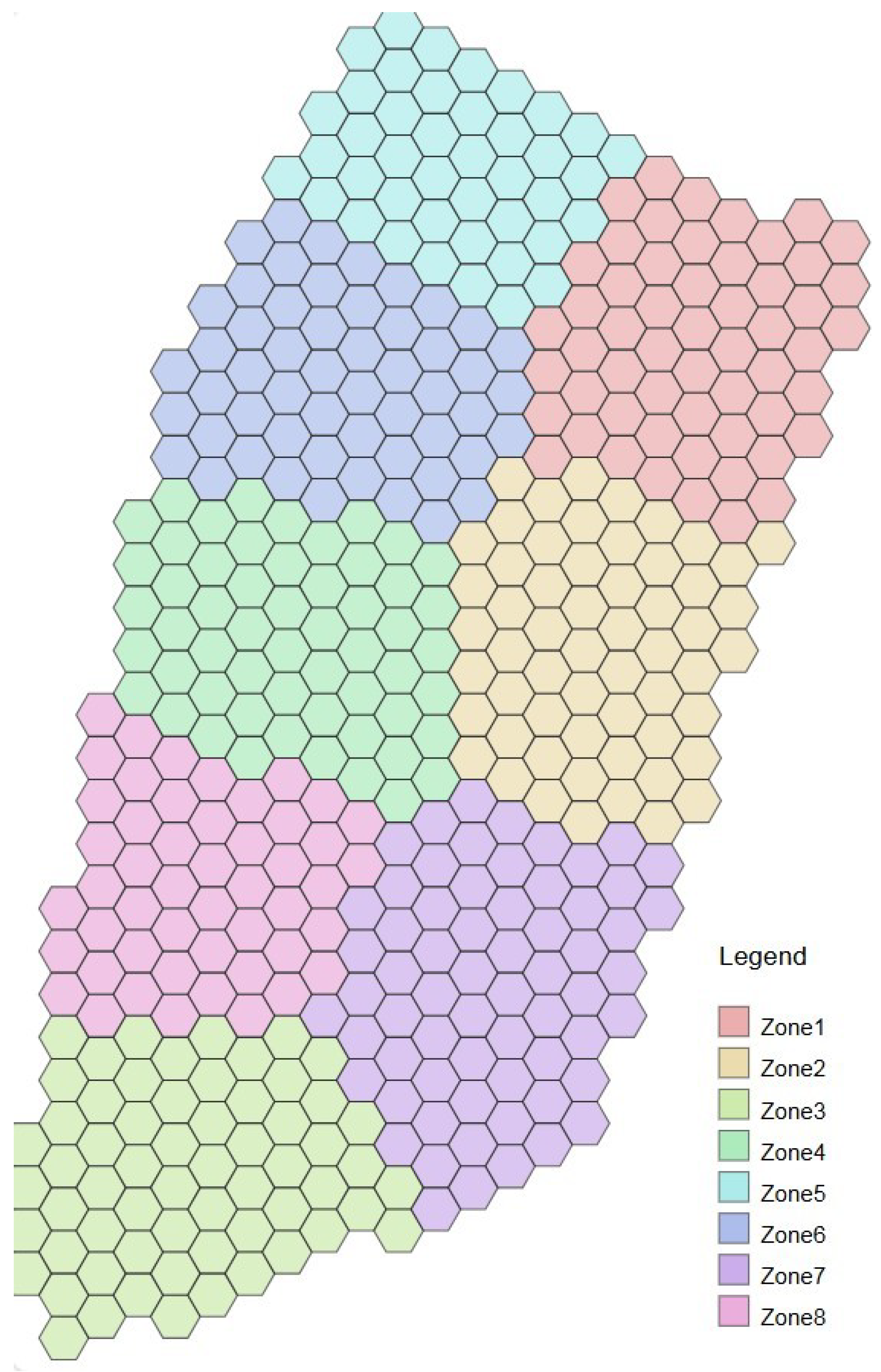
where , and is the linear intercept bounding the network scale (with and ). Any road segments falling outside this linear spatial cut-off are discarded. To maintain network connectivity, we manually pruned isolated nodes and disconnected streets. The operating area is partitioned into eight distinct zones [31], as illustrated in Figure 3.
Figure 3.
Network zoning map south of 60th Street in Manhattan.
To make the raw GPS coordinates compatible with distance calculation and spatial rendering, the geographic coordinates are transformed into a localized, positive-valued planar Cartesian coordinate system. Using a top-left benchmark point defined by base Latitude = 40.8 and base Longitude = −74, the planar coordinates x and y are calculated as:
where and are the minimum values among the filtered nodes, shifting the coordinate origin of the network to (0,0).
Nodes are generated at road intersections, and directed links are constructed to represent road segments. Since raw OpenStreetMap data lacks lane number information, lane numbers are systematically allocated based on road classification: motorways and motorway links are assigned three lanes, primary and primary links are assigned four lanes, and other road types default to one lane. The dynamic vehicle capacity of each link is calculated as a function of the lane count, segment length, vehicle length, and a safe following distance:
If the calculated capacity of an extremely short segment is zero, it is set to a default value of one. Bidirectional links are modeled by building a corresponding backward link with reversed start/end nodes and reversed coordinate vertex sequences, maintaining identical length and capacity as the forward link. This detailed topological network serves as the operational platform for evaluating the rebalancing strategies.
- (2)
- Travel demand.
The travel demand profiles used to drive our simulation are extracted from the real-world taxi trip records of the New York City Taxi and Limousine Commission (TLC) for January 2021 [28]. The raw dataset includes Yellow and Green taxi trip records, which capture detailed trip-level variables such as pickup and drop-off timestamps, travel distances, and taxi zone location identifiers for both passenger origins and destinations. To construct a consistent and clean travel demand profile for the Manhattan study area, we first exclude any trips with incomplete or missing data fields, and retain only those records whose pickup and drop-off location identifiers correspond to the active zones of our Manhattan road network. To synthesize a representative 24 h travel demand profile while preserving the daily cyclical transit patterns, the pickup timestamps of trips across a specified date range (from a defined start day to an end day in January) are aggregated, and their exact hours, minutes, and seconds are mapped onto a standardized single-day 24 h timeline. Additionally, travel distances are converted from miles to kilometers. Because the raw TLC taxi records only specify coarse taxi zone IDs rather than exact coordinates on the streets, we develop a spatial mapping mechanism to distribute this regional demand onto the micro-level road network links.
For each filtered trip, we identify all candidate origin and destination links situated within the respective pickup and drop-off taxi zones. To ensure operational feasibility for SAV routing and prevent vehicle congestion on narrow lanes, we restrict the candidate links to major roads with a capacity greater than or equal to a predefined threshold (set to 5). From these eligible candidates, a single origin link is selected randomly, with its selection probability weighted proportionally by the link lengths. The exact pickup coordinate along the selected origin link is then determined using a uniform distribution across its length. A symmetric mapping process is executed to determine the destination link and coordinate within the drop-off zone, ensuring that the origin and destination links are not identical. Through this hierarchical filtering and spatial mapping process, a continuous, micro-level demand dataset is constructed to evaluate fleet rebalancing.
- (3)
- Supply-side operational parameters.
Based on the minimum wage standards of New York State, passenger travel time is set to be USD 30 per hour for waiting and USD 15 per hour for travel time. A threshold of 10 min is established for passenger waiting; exceeding this duration classifies the customer as “unsatisfied,” triggering an operational penalty equivalent to ten times the expected in-vehicle transit cost. A fleet comprising 3000 SAVs is deployed in our simulation experiments. The fleet size is assumed to be 3000 SAVs and they are rebalanced by the operator every 20 min (i.e., min). This selected fleet size is determined through experimental testing to maintain high service quality and replicate realistic operational demands. Following the sensitivity findings of Loeb et al. [32], we assume that the AMoD service is not affected by vehicle battery capacity. We calibrate the daily SAV rental expense at a fixed rate of USD 50. By combining the economic analyses from Loeb and Kockelman [32,33] and Bauer et al. [34] with the 2022 Manhattan utility rates [35], we estimate the total operating cost—covering both maintenance and fleet management—to be USD 0.24 per kilometer.
The simulation model is implemented in C#, the deep learning model in Python (Version 3.8), and dispatch optimization is solved with Gurobi Version 10.0.1. All experiments are performed on a laptop with an Intel Core i5-8265U processor (1.80 GHz, 8 GB RAM). To account for system stochasticity, each scenario is executed across 10 independent simulation runs, and all reported performance metrics are presented as the mean ± standard deviation.
5.2. Basic Model Results
In this section, we use experiments to illustrate the performance of the proposed method with the FF rebalancing policy (baseline) and a standalone LSTM model.
5.2.1. Demand-Side Analysis
The trip of an AMoD service user typically progresses through four phases: submitting a travel request, receiving a dispatch assignment, pickup and in-vehicle travel, and finally arriving at the destination. To achieve a more granular evaluation of passenger wait times, we segment the pre-trip duration into two distinct, quantifiable metrics: assignment wait time, which spans from request submission to vehicle matching, and pickup wait time, which covers the interval from assignment to actual boarding.
The performance comparison from the demand side is detailed in Table 2. The hybrid LSTM-BiGRU model achieves high efficiency in several temporal dimensions, leading to a reduction of in assignment wait time (reaching 57.29 s) and in in-vehicle travel time (reaching 787.13 s) relative to the FF baseline. Conversely, the standalone LSTM model experiences a minor increase in assignment wait time () but yields the highest reduction in pickup wait time (reaching 160.30 s).
Table 2.
Passenger time costs and service quality under different rebalancing strategies.
However, analyzing the temporal metrics alone is insufficient, as aggressive fleet rebalancing can negatively affect service coverage. As shown in Table 2, both deep learning models result in an increase in the total number of unsatisfied passengers compared to the FF baseline, illustrating a key trade-off between localized supply–demand coordination and global service coverage. Specifically, the standalone LSTM model leads to a substantial surge in unsatisfied passengers (reaching 8817), whereas the proposed LSTM-BiGRU model limits this increase to only (reaching 7718, representing 444 additional unsatisfied passengers compared to FF). This indicates a systemic tendency of deep learning surrogates to prioritize areas with high demand density, occasionally bypassing peripheral low-demand zones. Nonetheless, by incorporating bidirectional gated recurrent units, the proposed LSTM-BiGRU framework captures broader context more effectively than the standalone LSTM, thereby achieving a significantly better operational balance between high temporal efficiency and robust service coverage.
5.2.2. Supply-Size Analysis
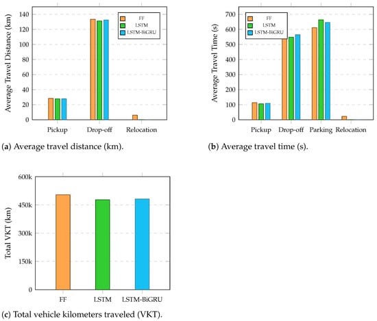
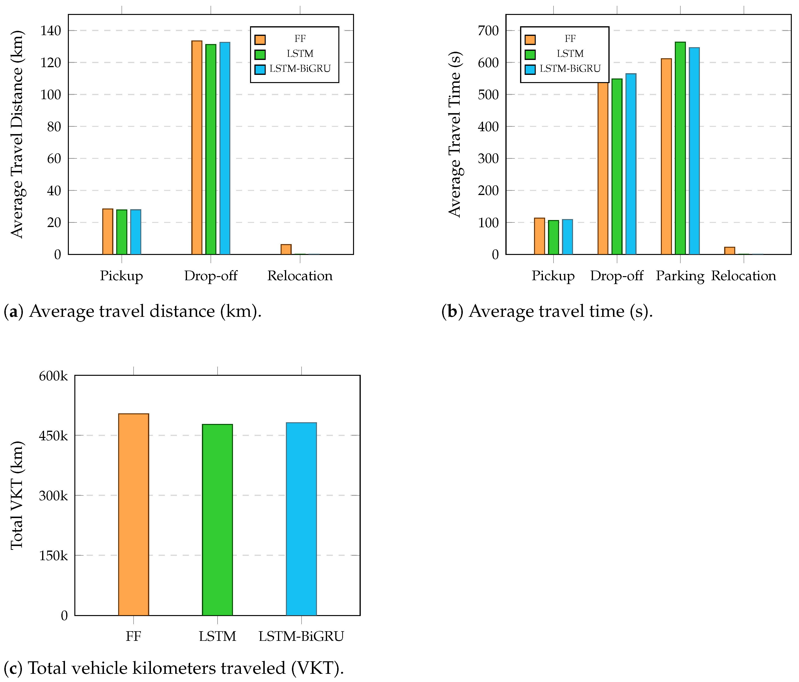
This subsection shows how rebalancing strategies affects the fleet performance. The average travel distance and duration of the SAV fleet, categorized by operational phases, are illustrated in Figure 4a,b. Both deep learning models achieve significant mileage and time optimizations during the active vehicle phases. Specifically, the LSTM-BiGRU framework reduces the average pickup duration from 113.2 s to 108.7 s (a −3.98% improvement) and saves 0.5 km in average pickup distance, reflecting superior positioning of vehicles prior to demand arrival. This optimization extends to empty vehicle relocations; both neural network models nearly eliminate the inefficient cross-zone deadheading, reducing average relocation distance from 6.1 km (FF) to just 0.1 km, and virtually wiping out vacant transit times. Concurrently, the reduction in unnecessary travel leads to an increase in vehicle parking times, with the LSTM-BiGRU model experiencing a +5.64% rise in average idling duration. This increase indicates that empty vehicles remain parked at designated stations in anticipated high-demand zones rather than continuously wandering or executing redundant cross-zone movements, thereby reducing street congestion and saving fleet energy.
Figure 4.
Average travel time, distance, and total VKT comparison for different strategies.
Figure 4c shows the total vehicle kilometers traveled (VKT) across the entire fleet under the three strategies. Compared to the FF baseline (503,907 km), the LSTM-BiGRU framework achieves a substantial reduction of −4.41% in total VKT, saving 22,247 km of travel. Although the standalone LSTM model achieves an even greater reduction in total mileage (−5.29%, reaching 477,202 km), it does so by relying on short-term local rebalancing, which results in a severe loss of passengers as previously analyzed.
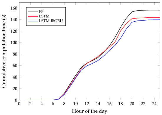
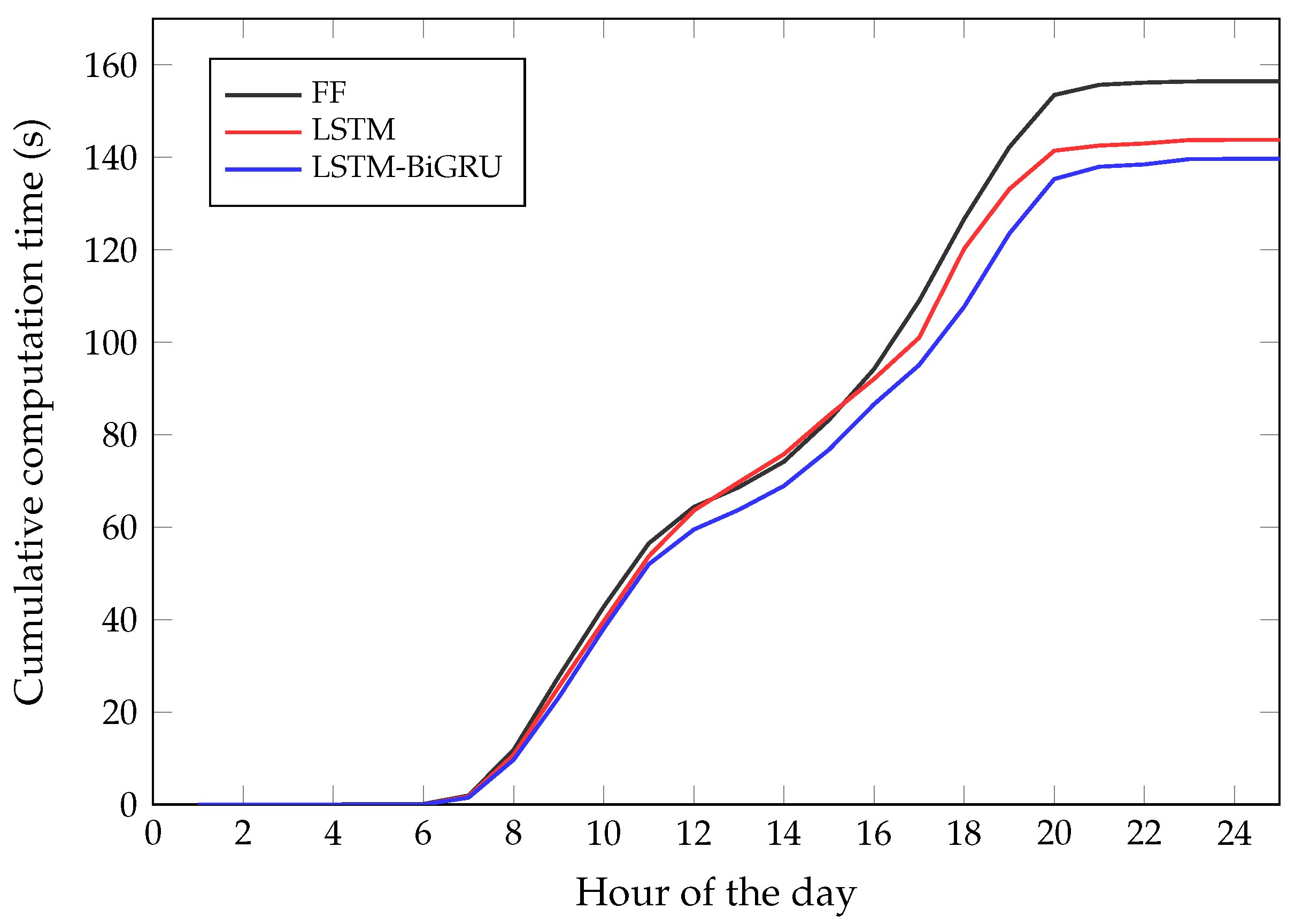
5.2.3. Computation Time
This subsection investigate the computation time of the strategies. Figure 5 depicts the cumulative computation time of a simulation day. During the initial off-peak operational phase (1:00–6:00), extremely low travel demand allows all three methods to generate rebalancing decisions almost instantaneously, resulting in negligible computational delays. However, as travel requests surge throughout the day, the computational advantage of the deep learning surrogate approach becomes prominent. At 10:00, the baseline FF strategy requires 42.78 s to compute dispatch commands, whereas the LSTM-BiGRU model completes the same task in 38.08 s, marking a 10.98% reduction in decision-making time. The most substantial performance divergence occurs during the evening peak at 18:00, where the LSTM-BiGRU framework reduces the computation time by 18.98 s (a 14.98% speed-up) compared to the mathematical FF model.
Figure 5.
Cumulative computation time across a simulation day.
It is worth noting that a clear distinction must be made among individual neural network inference latency, per-step simulation overhead, and cumulative system-level computational time. The online forward pass of our trained LSTM-BiGRU surrogate model takes only 15 milliseconds (0.015 s) on average to generate a single relocation matrix . In contrast, the decision times reported in Figure 5 represent the cumulative computational time over the entire 24 h simulation day (comprising 75 dispatch steps), which includes both the neural network inference time and the real-time state extraction and data aggregation overhead within the simulation engine. This results in an average system-level overhead of approximately 1.86 s per step. In comparison, the mathematical FF model solved via Gurobi experiences severe latency spikes during peak traffic hours, taking up to 126.67 s for a single decision step at 18:00, whereas the neural network’s inference latency remains strictly constant at 15 milliseconds, proving its real-time operational feasibility.
5.3. Benefits of Incorporating Congestion Effects During Rebalancing
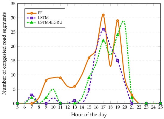
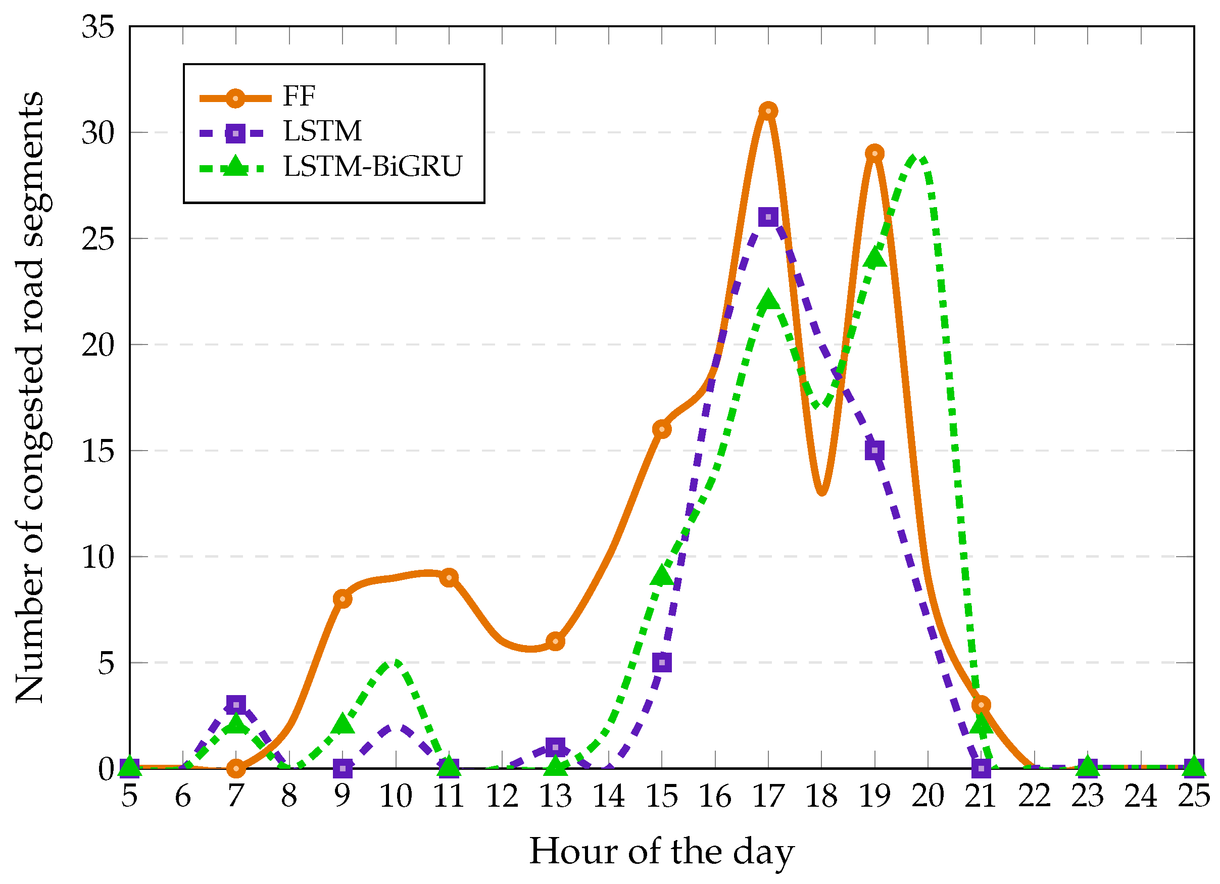
This subsection analyzes the hourly variations in traffic congestion under the strategies. Figure 6 illustrates the distribution of congested road segments throughout a 24 h simulation cycle.
Figure 6.
Number of congested road segments per hour.
The baseline FF strategy suffers from severe peak-hour performance degradation due to its static flow assumptions. As shown in Figure 6, FF generates the highest number of congested road links during peak periods, reaching a maximum of 31 congested segments at 17:00. This spike reflects its inability to adapt dynamically to high concurrent demand. During early off-peak hours (1:00–6:00), all three strategies perform identically with zero congested segments, indicating that the baseline model is only suitable for low-demand environments.
The standalone LSTM model offers the most substantial reduction in overall traffic congestion, cutting the total number of congested links by 42.35% compared to the FF baseline. This model maintains minimal congestion levels throughout the mid-day period. However, as detailed in our earlier service quality evaluation, this congestion mitigation comes at a significant cost to passenger satisfaction, resulting in 8817 unsatisfied customers. This highlights a critical operational trade-off where the LSTM model aggressively restricts vehicle rebalancing to preserve road network efficiency at the expense of passenger service coverage.
In comparison, the proposed LSTM-BiGRU framework represents a more balanced solution, achieving a 25.29% overall reduction in road congestion while maintaining a significantly higher level of service. During peak periods, the hybrid model performs robustly, experiencing only 22 congested links at 17:00 compared to FF’s 31. Although a minor congestion spike of 28 links is observed at 20:00, possibly due to the bidirectional architecture’s persistent focus on late-evening transit demand, the total unsatisfied passenger count is restricted to 7718 (only a minor 6.10% increase over FF). This confirms that the proposed deep learning-based framework successfully balances urban traffic efficiency with robust service coverage.
5.4. Effects of SAV Fleet Size
This subsection shows how the fleet size () affects the operational efficiency and service viability of an AMoD system. To evaluate the scalability and performance boundaries of the proposed model under different supply levels, we vary the fleet size from 2000 to 4000 SAVs in increments of 500 while keeping the dispatch interval fixed at min.
Table 3 compares the performance indicators. A clear operational trade-off emerges as the fleet size scales up. From the service quality perspective, a restricted fleet size of represents a severe undersupply scenario, where the system suffers from an average passenger wait time of 295.42 s and a large number of unsatisfied passengers (15,240), indicating that the available vehicle supply cannot cover spatial demand even under the optimized rebalancing policy. Increasing the fleet size to dramatically improves AMoD system performance, reducing wait times to 185.12 s and cutting unsatisfied passengers to 3115. Conversely, scaling up the fleet inevitably generates resource redundancy and increases idle capacity. The average vehicle parking time surges by 188% (rising from 342.1 s at to 985.6 s at ), while the total operational cost increases linearly from USD 176,578 to USD 358,420 due to the accumulation of daily rental expenses and empty VKT. These competing trends indicate that a fleet size of represents a pragmatic socio-economic equilibrium for Manhattan operations, balancing passenger wait times and operational deficits.
Table 3.
System performance under different fleet sizes ().
5.5. Effects of the Rebanlancing Interval
To systematically evaluate the robustness of the proposed LSTM-BiGRU model, we examine the system performance fluctuations under different rebalancing intervals. We vary the rebalancing interval min while maintaining the fleet size at SAVs.
Table 4 presents the operational results. A shorter dispatch interval of min increases the decision granularity, allowing the LSTM-BiGRU surrogate model to execute rebalancing decisions more frequently. This leads to the lowest average passenger wait time (206.15 s) and the minimum unsatisfied passenger count (6115). However, such high frequency triggers a substantial number of micro-relocations, causing the total empty mileage to rise to 128,940 km and increasing the cumulative peak-hour decision-making time to 168.32 s. Conversely, a longer dispatch interval of min leads to delayed system responsiveness. The lag in empty vehicle redistribution causes passenger wait times to rise to 245.85 s and unsatisfied passengers to surge to 9980, although it yields the lowest empty VKT (94,150 km) and total operational cost (USD 255,120). These competing trends prove that our selection of min successfully balances computational demand, empty mileage, and passenger satisfaction, serving as a highly effective operational parameter for the system.
Table 4.
System performance under different dispatch intervals ().
6. Discussion
The experimental evaluations show that the proposed LSTM-BiGRU framework provides operational improvements in travel times, decision-making latency, and fleet-wide mileage compared to the mathematical rebalancing model. However, the underlying system interactions and trade-offs within the simulated AMoD environment warrant deeper discussion.
6.1. Trade-Off Between System Efficiency and Social Equity
Although the LSTM-BiGRU model reduces total travel times and vehicle miles, it simultaneously results in a 6.10% increase in unsatisfied passengers (corresponding to 444 additional travelers). This phenomenon reveals an inherent trade-off between global fleet optimization and spatial service equity.
When the deep learning model replaces the mathematical optimization baseline, it implicitly learns to prioritize high-density travel corridors, such as the core commercial zones of Manhattan, to maximize vehicle turnover rates and minimize vacant relocation mileage. Consequently, idle vehicles are concentrated in high-demand zones, leaving peripheral or lower-demand zones underserved. This spatial bias explains the localized congestion spike observed at 20:00, where vehicles over-concentrated during the evening peak transition. In real-world commercial SAV deployment, such spatial inequity could lead to user dissatisfaction in peripheral neighborhoods. This indicates that future model objectives or loss functions should incorporate spatial fairness constraints alongside operational efficiency.
To support this spatial equity analysis, we extracted zone-level operational metrics from our simulation runs. The core commercial areas (Zones 1–3) account for approximately 65% of the total Manhattan travel demand, and under our deep learning framework, they receive highly concentrated vehicle relocation inflows, resulting in a low average passenger wait time of approximately 145 s. In contrast, the peripheral low-demand areas (Zones 7 and 8) account for less than 8% of the total demand, and because the neural surrogate prioritizes high-demand corridors to maximize fleet-wide efficiency, empty vehicles are rarely relocated to these areas. Consequently, average passenger wait times in these peripheral zones rise to approximately 320 s, and the 444 additional unsatisfied passengers are heavily clustered in Zones 7 and 8.
6.2. Modeling in Complex Systems Engineering
In systems engineering, computational feasibility is as critical as optimality, while mathematical optimization models, such as the FF strategy solved via Gurobi, yield optimal solutions under static assumptions, their execution time scales heavily with fleet size V and spatial partitions, presenting challenges for real-time online deployment.
By training the LSTM-BiGRU network on simulation-generated dispatch data, the framework acts as an efficient surrogate model. It shifts the computational burden of optimization to offline training. During online deployment, the vehicle rebalancing decision is reduced to a near-instantaneous neural network forward pass, yielding a 10.73% reduction in cumulative decision-making time even during peak concurrent request periods. This demonstrates that hybrid deep learning–simulation paradigms offer a pragmatic path toward scalable and responsive AMoD control systems. Consequently, the novelty of our neural surrogate lies not in altering the mathematical optimality of the offline baseline, but in enabling its near-instantaneous online execution and robust generalization under dynamic system states.
Additionally, the selection of an eight-zone spatial partition represents a mathematically optimal scale for Southern Manhattan. Partitioning this compact region into 100+ zones would lead to severe zero-inflation in travel demand and vehicle idle counts per interval. Such high-dimensional sparsity would introduce significant statistical noise into the optimization, causing fleet relocation actions to oscillate and become operationally meaningless, while simultaneously increasing the neural network’s output dimension to an intractable 10,000-dimensional space.
7. Conclusions
This paper proposes a deep learning-based approach for SAV rebalancing problem by integrating a cascaded LSTM-BiGRU deep learning network with a congestion-aware discrete event simulation model. By offline-training the neural network to imitate the relocation rules of a traditional mathematical optimization model, the proposed framework successfully shifts the massive computational burden of real-time mathematical programming to offline learning, enabling sub-second decision responsiveness online.
Based on the system-level simulation experiments conducted on the Manhattan road network, we obtain the following findings. Compared to the traditional decoupled predict-then-optimize baseline (FF solved via Gurobi), the proposed deep learning-based framework achieves notable gains in execution speed. During peak-demand periods, the surrogate model reduces dispatch decision latency by 13.86 to 18.98 s. Under sustained high loads, it maintains a robust average decision time of 139.67 s (representing a 10.73% and 2.63% reduction compared to the FF baseline and standalone LSTM model, respectively), demonstrating its computational viability for real-time, large-scale urban AMoD operations. The surrogate framework achieves significant resource savings, reducing total fleet vehicle mileage by 22,247 km (−4.41%) and lowering overall vehicle operational costs by USD 5339 (−1.97%). However, the evaluation reveals a critical systemic trade-off. That is, the global optimization bias of the surrogate network leads to a 6.10% increase in unsatisfied passengers (+444) and localized congestion spikes around 20:00, highlighting the inherent tension between global operational efficiency and spatial service equity. Sensitivity analysis confirms that the proposed approach remains robust and scalable across varying system states. A fleet size of SAVs paired with a dispatch interval of min represents a pragmatically optimized socio-economic equilibrium for Manhattan’s urban mobility network, successfully balancing computational overhead, vehicle empty VKT, and passenger wait times.
The findings of this study have profound implications for urban environmental and socio-economic sustainability. By enabling real-time, highly responsive SAV rebalancing, the proposed deep learning-based surrogate framework directly mitigates the dynamic traffic congestion that plagues modern metropolitan areas. Specifically, the demonstrated 25.29% reduction in road congestion and the 22,247 km decrease in empty vehicle travel (VKT) translate directly into lower fuel consumption, reduced greenhouse gas emissions, and a smaller carbon footprint for the shared mobility fleet. From an economic perspective, reducing unnecessary relocation travel saves operational costs while improving passenger wait times, thereby promoting public acceptance of shared, on-demand automated transit as a resource-efficient alternative to private vehicle ownership. This work provides valuable decision-making support for city planners and SAV fleet operators striving to transition toward green, low-carbon, and highly responsive smart city transportation networks.
Despite these promising findings, several avenues remain for future research. First, to mitigate the observed spatial service gaps and equity issues, future work will focus on integrating attention mechanisms and spatial fairness constraints directly into the neural network’s loss function. Second, implementing dynamic, demand-elastic fleet sizing policies, incorporating V2X communication latency constraints, and integrating graph neural networks (GNNs) for high-resolution spatial partitioning will further enhance the model’s robustness and scalability in real-world deployments.
Author Contributions
Conceptualization, J.Y.; methodology, J.Y.; validation, J.Y.; formal analysis, J.Y.; investigation, J.Y. and J.L.; resources, J.Y. and Y.D.; data curation, J.Y.; writing—original draft preparation, J.Y.; writing—J.Y.; visualization, J.Y.; supervision, J.Y.; project administration, J.Y.; funding acquisition, J.Y. All authors have read and agreed to the published version of the manuscript.
Funding
This work was partially supported by the Humanities and Social Sciences Cultivation Project of Kunming University of Science and Technology (Grant No. SKPYYB202407), the National Natural Science Foundation of China (Grand No. 72471200, 52562049), the Scientific Research Fund for Yunnan Provincial Department of Education [Grant No. 2025J0110], and the Fundamental Research Program in Yunnan Province [Grant No. 202501AU070100].
Institutional Review Board Statement
Not applicable.
Informed Consent Statement
Not applicable.
Data Availability Statement
The data supporting the findings of this study are available from the corresponding author upon reasonable request.
Acknowledgments
The authors would like to thank the anonymous reviewers for their comments and suggestions that helped to improve the quality of this manuscript.
Conflicts of Interest
The authors declare no conflicts of interest.
Abbreviations
The following abbreviations are used in this manuscript:
| SAV | Shared Autonomous Vehicle |
| AMoD | Automated Mobility-on-Demand |
| DES | Discrete Event Simulation |
| LSTM | Long Short-Term Memory |
| BiGRU | Bidirectional Gated Recurrent Unit |
| MILP | Mixed-Integer Linear Programming |
| MPC | Model Predictive Control |
| DQN | Deep Q-Network |
| TLC | Taxi and Limousine Commission |
References
- Bösch, P.M.; Becker, F.; Becker, H.; Axhausen, K.W. Cost-based analysis of autonomous mobility services. Transp. Policy 2018, 64, 76–91. [Google Scholar] [CrossRef] [Scilit]
- Lin, Y.; Zhang, K.; Kondor, D.; Zhao, Z.; Ratti, C.; Xu, Y. Exploring influential factors of fleet and parking management in shared autonomous vehicle systems: An agent-based simulation framework. Transp. Res. Part A Policy Pract. 2025, 203, 104762. [Google Scholar] [CrossRef] [Scilit]
- Anderson, J.M.; Nidhi; Stanley, K.D.; Sorensen, P.; Samaras, C.; Oluwatola, O.A. Autonomous Vehicle Technology: A Guide for Policymakers. Rand Corporation Technical Report. 2014. Available online: https://www.rand.org/pubs/research_reports/RR443-2.html (accessed on 12 June 2026).
- Tirachini, A.; Gomez-Lobo, A. Does ride-hailing increase or decrease vehicle kilometers traveled (VKT)? A simulation approach for Santiago de Chile. Int. J. Sustain. Transp. 2020, 14, 187–204. [Google Scholar] [CrossRef] [Scilit]
- Pavone, M.; Smith, S.L.; Frazzoli, E.; Rus, D. Load Balancing for Mobility-on-Demand Systems. Int. J. Robot. Res. 2012, 31, 839–854. [Google Scholar] [CrossRef] [Scilit]
- Smith, S.L.; Pavone, M.; Schwager, M.; Frazzoli, E.; Rus, D. Rebalancing the Rebalancers: Optimally Routing Vehicles and Drivers in Mobility-on-Demand Systems. In Proceedings of the 2013 American Control Conference, Washington, DC, USA, 17–19 June 2013; pp. 2362–2367. [Google Scholar]
- Zhang, R.; Pavone, M. Control of Robotic Mobility-On-Demand Systems: A Queueing-Theoretical Perspective. Int. J. Robot. Res. 2014, 35, 186–203. [Google Scholar] [CrossRef] [Scilit]
- Kek, A.G.H.; Cheu, R.L.; Meng, Q.; Fung, C.H. A decision support system for vehicle relocation operations in carsharing systems. Transp. Res. Part E Logist. Transp. Rev. 2009, 45, 149–158. [Google Scholar] [CrossRef] [Scilit]
- Qian, X.; Zhan, X.; Ukkusuri, S.V. Characterizing Urban Dynamics Using Large Scale Taxicab Data; Springer International Publishing: Berlin/Heidelberg, Germany, 2015. [Google Scholar]
- Miao, F.; Lin, S.; Munir, S.; Stankovic, J.A.; Pappas, G.J. Taxi Dispatch with Real-Time Sensing Data in Metropolitan Areas—A Receding Horizon Control Approach. In Proceedings of the ACM/IEEE Sixth International Conference on Cyber-Physical Systems, Seattle, WA, USA, 13–15 April 2015; pp. 1–10. [Google Scholar]
- Iglesias, R.; Rossi, F.; Wang, K.; Hallac, D.; Leskovec, J.; Pavone, M. Data-driven model predictive control of autonomous mobility-on-demand systems. In Proceedings of the 2017 IEEE International Conference on Robotics and Automation (ICRA), Singapore, 29 May–3 June 2017; pp. 3005–3012. [Google Scholar]
- Wen, J.; Zhao, J.; Jaillet, P. Rebalancing shared mobility-on-demand systems: A reinforcement learning approach. In Proceedings of the 2017 IEEE 20th International Conference on Intelligent Transportation Systems (ITSC), Yokohama, Japan, 16–19 October 2017; pp. 220–225. [Google Scholar]
- Fagnant, D.J.; Kockelman, K.M. The travel and environmental implications of shared autonomous vehicles, using agent-based model scenarios. Transp. Res. Part C Emerg. Technol. 2014, 40, 1–13. [Google Scholar] [CrossRef] [Scilit]
- Zhang, Z.; Liu, J.; Nie, Q.; Jones, S. Shared low-speed autonomous vehicles for short-distance trips: Agent-based modeling with mode choice analysis. Transp. Plan. Technol. 2025, 48, 313–341. [Google Scholar] [CrossRef] [Scilit]
- Karolemeas, C.; Tsigdinos, S.; Moschou, E.; Kepaptsoglou, K. Shared autonomous vehicles and agent based models: A review of methods and impacts. Eur. Transp. Res. Rev. 2024, 16, 25. [Google Scholar] [CrossRef] [Scilit]
- Yang, J.; Zeng, R.; Du, Y. Evaluating shared autonomous vehicles through agent-based discrete event simulation. J. Simul. 2026, 1–21. [Google Scholar] [CrossRef] [Scilit]
- Gumahad, B.; Collins, A.J. Comparing Simulated Autonomous Swarm Systems using Agent-Based Modeling. In Proceedings of the 2024 Annual Modeling and Simulation Conference (ANNSIM), Washington, DC, USA, 20–23 May 2024; pp. 1–12. [Google Scholar]
- Pizarro, V.; Leger, P.; Hidalgo-Alcázar, C.; Figueroa, I. ABM RoutePlanner: An agent-based model simulation for suggesting preference-based routes in Spain. J. Simul. 2023, 17, 444–461. [Google Scholar] [CrossRef] [Scilit]
- Hörl, S.; Ruch, C.; Becker, F.; Frazzoli, E.; Axhausen, K.W. Fleet operational policies for automated mobility: A simulation assessment for Zurich. Transp. Res. Part C Emerg. Technol. 2019, 102, 20–31. [Google Scholar] [CrossRef] [Scilit]
- Yang, Y.; Fu, X.; Zhang, L. Electric autonomous vehicle fleet scheduling and charging station placement optimization. Transp. Sci. 2020, 54, 892–907. [Google Scholar]
- Yang, J.; Levin, M.W.; Hu, L.; Li, H.; Jiang, Y. Fleet sizing and charging infrastructure design for electric autonomous mobility-on-demand systems with endogenous congestion and limited link space. Transp. Res. Part C Emerg. Technol. 2023, 152, 104172. [Google Scholar] [CrossRef] [Scilit]
- Hassannayebi, E.; Memarpour, M.; Mardani, S.; Shakibayifar, M.; Bakhshayeshi, I.; Espahbod, S. A hybrid simulation model of passenger emergency evacuation under disruption scenarios: A case study of a large transfer railway station. J. Simul. 2020, 14, 204–228. [Google Scholar] [CrossRef] [Scilit]
- Yang, J.; Hu, L.; Jiang, Y.; Yang, T. Simulation-based design of multi-period bus headways under the influence of electronic bus station boards. J. Simul. 2022, 16, 339–354. [Google Scholar] [CrossRef] [Scilit]
- He, Z.; Song, Q.; Lian, J.; Liu, Y. Towards Standardizing Validation Practices in Agent-Based Modeling: A Hierarchical ABM Validation Framework. ACM Trans. Model. Comput. Simul. 2025, 36, 1–25. [Google Scholar] [CrossRef] [Scilit]
- Bischoff, J.; Maciejewski, M. Simulation of City-wide Replacement of Private Cars with Autonomous Taxis in Berlin. Procedia Comput. Sci. 2016, 83, 237–244. [Google Scholar] [CrossRef] [Scilit]
- Li, T.; Levin, M.W.; Boyles, S.D.; Kockelman, K. A general framework for modeling shared autonomous vehicles with dynamic network-loading and dynamic ride-sharing application. Comput. Environ. Urban Syst. 2017, 64, 373–383. [Google Scholar] [CrossRef] [Scilit]
- Zhang, H.; Sheppard, C.J.R.; Lipman, T.E.; Moura, S.J. Joint Fleet Sizing and Charging System Planning for Autonomous Electric Vehicles. IEEE Trans. Intell. Transp. Syst. 2020, 21, 4711–4721. [Google Scholar] [CrossRef] [Scilit]
- New York City Taxi and Limousine Commission. TLC Trip Record Data. Available online: https://www.nyc.gov/site/tlc/about/tlc-trip-record-data.page (accessed on 17 July 2021).
- Beck, M.; Pöppel, K.; Spanring, M.; Auer, A.; Prudnikova, O.; Kopp, M.; Klambauer, G.; Brandstetter, J.; Hochreiter, S. xLSTM: Extended long short-term memory. Adv. Neural Inf. Process. Syst. 2024, 37, 107547–107603. [Google Scholar] [CrossRef] [Scilit]
- Fu, R.; Zhang, Z.; Li, L. Using LSTM and GRU neural network methods for traffic flow prediction. In Proceedings of the 2016 19th International Conference on Information Fusion (FUSION), Heidelberg, Germany, 5–8 July 2016; pp. 321–328. [Google Scholar]
- Apte, M.; Agarwadkar, Y.Y.Y.; Azmi, S.; Inamdar, A.B. Understanding Grids and Effectiveness of Hexagonal Grid in Spatial Domain. In Proceedings of the Second International Conference on Recent Trends in Information Technology and Computer Science (ICRTITCS-2012), Mumbai, India, 7 February 2013. [Google Scholar]
- Loeb, B.; Kockelman, K.M.; Liu, J. Shared autonomous electric vehicle (SAEV) operations across the Austin, Texas network with charging infrastructure decisions. Transp. Res. Part C Emerg. Technol. 2018, 89, 222–233. [Google Scholar] [CrossRef] [Scilit]
- Loeb, B.; Kockelman, K.M. Fleet performance and cost evaluation of a shared autonomous electric vehicle (SAEV) fleet: A case study for Austin, Texas. Transp. Res. Part A Policy Pract. 2019, 121, 374–385. [Google Scholar] [CrossRef] [Scilit]
- Bauer, G.S.; Greenblatt, J.B.; Gerke, B.F. Cost, Energy, and Environmental Impact of Automated Electric Taxi Fleets in Manhattan. Environ. Sci. Technol. 2018, 52, 4920–4928. [Google Scholar] [CrossRef] [Scilit]
- New York State Energy Research and Development Authority. Charging Station Programs. Available online: https://www.nyserda.ny.gov/All-Programs/ChargeNY/ChargeElectric/Charging-Station-Programs/Charge-Ready-NY/ (accessed on 12 August 2022).

Disclaimer/Publisher’s Note: The statements, opinions and data contained in all publications are solely those of the individual author(s) and contributor(s) and not of MDPI and/or the editor(s). MDPI and/or the editor(s) disclaim responsibility for any injury to people or property resulting from any ideas, methods, instructions or products referred to in the content. |
© 2026 by the authors. Licensee MDPI, Basel, Switzerland. This article is an open access article distributed under the terms and conditions of the Creative Commons Attribution (CC BY) license.