


Abstract
Urban-scale road traffic noise mapping is frequently constrained by limited access to spatially continuous traffic observations, particularly in data-scarce cities. This study developed an integrated framework for reconstructing road-segment traffic activity from high-resolution satellite imagery and applying it to physical noise modeling in central Changshu, China. Vehicles were detected using YOLOv7, converted to centroid points, and assigned to road segments through class-specific spatial buffers. Snapshot vehicle density was combined with road-class-specific characteristic speeds to estimate flow-equivalent traffic activity, which was incorporated with road-network and building data into OpeNoise Map. Model outputs were evaluated against measured equivalent sound levels at 88 monitoring sites. Road-class statistics were calculated for both all eligible segments, including zero detections, and positive-detection segments only. Arterial roads exhibited the highest mean activity under both definitions, followed by expressways, while including zero-detection segments substantially reduced mean and median estimates, particularly for secondary roads. Predicted noise showed a pronounced road-dependent pattern, with high levels concentrated along expressways, arterial roads, and major intersections and decreasing toward interior urban blocks. Validation produced a mean bias of 1.29 dB, mean absolute error of 5.46 dB, root-mean-square error of 7.81 dB, Pearson correlation coefficient of 0.497, and R2 of 0.247. The small bias indicates limited overall systematic deviation, whereas the modest correlation and R2 demonstrate limited reproduction of site-level variability. The framework is therefore more suitable for reconstructing broad urban noise patterns, identifying potential high-noise corridors, and supporting preliminary spatial screening than for precise site-level prediction. It represents image–time conditions and should complement continuous traffic monitoring and statutory acoustic assessment, with calibration using multi-temporal imagery and synchronized ground observations.
1. Introduction
Rapid urbanization and increasing motorized mobility have intensified environmental pressures in cities, among which road traffic noise represents one of the most widespread and persistent sources of human exposure [1,2,3]. Unlike episodic industrial or construction noise, road traffic noise is closely coupled with the spatial organization of urban road networks and continuously affects residential, educational, commercial, and public spaces [4,5,6]. Accumulating epidemiological evidence has associated long-term environmental noise exposure with annoyance, sleep disturbance, cardiovascular and metabolic effects, psychological stress, and impaired cognitive development in children [7,8,9,10,11]. These impacts have shifted road traffic noise from a conventional environmental nuisance to an important public-health and spatial-planning concern. Reliable characterization of its spatial distribution is therefore essential not only for identifying high-exposure corridors, but also for supporting noise mitigation, land-use planning, transport management, and health-oriented urban design [12].
Urban traffic noise is inherently spatially heterogeneous because the sound level observed at a given location reflects the combined effects of source emission and propagation conditions [13,14]. At the source level, traffic volume, vehicle composition, speed, acceleration, pavement characteristics, road gradient, and intersection operations influence acoustic emission [15]. During propagation, source–receiver distance, building obstruction, façade reflection, diffraction, ground effects, and urban morphology further modify received sound levels [13,15,16]. Consequently, locations with similar traffic volumes may exhibit substantially different acoustic conditions because of variations in road configuration and the surrounding built environment [14,17,18]. This source–propagation interaction makes spatially explicit noise mapping particularly important in dense urban areas, where high-traffic roads, complex intersections, enclosed street spaces, and heterogeneous building configurations coexist over relatively short distances [17,18].
Existing approaches to characterizing urban noise can be broadly divided into field monitoring, sensor-network observation, statistical estimation, and physical acoustic modeling. Field measurements provide direct observations but are costly and labor-intensive at urban scales, and their temporal and spatial representativeness is limited [19,20]. Wireless acoustic sensor networks improve temporal continuity but depend on calibration, maintenance, and long-term operational stability [21]. Statistical approaches, including land-use regression and machine-learning models, estimate noise distributions from road, land-use, and other spatial variables [22,23], but their reliability depends on the quantity and transferability of monitoring samples, and they provide only an indirect representation of emission and propagation mechanisms [23,24]. Critically, none of these approaches directly supplies the road-segment traffic-activity inputs that high-spatial-resolution noise modeling requires.
Physical acoustic models offer a complementary capability by explicitly representing road-source emissions and propagation processes, including geometrical divergence, atmospheric absorption, ground interaction, building shielding, reflection, and diffraction [25]. Methods such as CNOSSOS-EU have been standardized and extensively validated, so the core bottleneck in urban noise assessment is no longer the acoustic model itself. The binding constraint is the source term: vehicle activity is the key input driving road-source emission, yet spatially continuous, low-cost, updatable, and comparable traffic-activity data across an entire road network remain largely unavailable [26,27,28]. While road geometry, building footprints, and heights can be obtained from open geographic platforms [28,29], dynamic traffic attributes—volume, speed, composition, and operating state—are substantially harder to acquire consistently at the city scale [30].
Traffic activity is commonly characterized using fixed counters, roadside cameras, floating-car or probe-vehicle data, mobile-phone mobility records, manual surveys, or calibrated transport-model outputs [31]. Recent deep-learning studies have advanced spatial–temporal traffic forecasting through joint pre-training, as exemplified by JointSTNet [32]; however, such methods rely on continuous historical traffic observations rather than snapshot data. All of these sources face practical constraints for high-resolution noise modeling: fixed sensors cover only selected road sections, manual surveys are difficult to scale, trajectory and traffic-management data may be proprietary, and network-wide models require extensive calibration [15,30,33,34]. Consequently, conventional traffic surveys rarely support segment-level noise modeling across a full urban network, a limitation that is particularly pronounced in data-scarce cities [5,35].
Earth observation provides a potential new data source for addressing this gap [36,37]. Satellite imagery offers synoptic coverage and a standardized observation geometry that is not restricted to preselected ground-monitoring locations. Medium-resolution data have been used to detect moving trucks and characterize broad freight patterns [36], while high-resolution satellite and aerial imagery has supported individual vehicle detection, truck-activity estimation, and spatially extensive traffic information extraction [38,39]. These developments indicate that Earth observation can complement ground-based monitoring by improving spatial coverage, particularly where network-wide observations are unavailable.
Advances in deep-learning-based object detection, including the YOLO family and dedicated aerial-vehicle datasets, have further enabled the automated extraction of small vehicles from high-resolution imagery [40,41]. City-scale applications have demonstrated road-level vehicle detection from satellite imagery, while also revealing persistent difficulties associated with narrow streets, building shadows, vegetation occlusion, and image quality [42]. Nevertheless, these studies still face limitations related to image acquisition frequency and the need for validation against ground-based observations [36,42].
More fundamentally, detecting vehicles in a satellite image does not directly produce the traffic parameters required by an acoustic model [13]. A satellite image records the instantaneous spatial occupancy of vehicles, whereas traffic flow is a temporal rate describing the number of vehicles passing a road section during a defined interval [43]. Converting the former into the latter requires at least three additional operations: assigning each detected vehicle to the correct road segment, deriving road-segment vehicle density, and linking density to flow through an assumed or independently estimated speed [39]. Each of these operations introduces uncertainty—through assignment ambiguity, zero-detection segments, and class-level speed assumptions—yet the cumulative effect of this conversion chain on the accuracy of the resulting noise predictions has rarely been quantified against field measurements [44]. Consequently, remote-sensing-derived traffic parameters should be regarded as snapshot-based estimates or proxies unless they are calibrated and validated using ground observations.
Although previous research has separately advanced satellite vehicle detection [42,45], traffic characterization [15], and urban noise modeling [29,46], the operational linkage among these components remains insufficiently developed. Most remote-sensing vehicle studies terminate at the detection, counting, or speed-estimation stage, without translating their outputs into spatially explicit acoustic source inputs [36,39,42]. Conversely, many physical noise-mapping studies assume that traffic volumes and speeds are already available from surveys, fixed monitoring systems, or transport models [26,28]. Therefore, the unresolved research gap is not simply the detection of vehicles or the application of an acoustic model. It is the lack of a transparent and reproducible workflow that converts spatially extensive but temporally discrete vehicle observations into road-segment traffic-activity parameters, links these parameters to physical acoustic source inputs, and evaluates the resulting noise predictions against field observations [47]. Addressing this gap is necessary to determine both the practical value and the limitations of satellite imagery for traffic-noise mapping in cities with incomplete traffic data.
To address this problem, this study develops an integrated framework for urban road traffic noise mapping using high-resolution satellite imagery, road network data, building information, and field noise observations. The central urban area of Changshu, China, is selected as the study area. Vehicles are first detected from road-region imagery using an established deep-learning model. Their geometric centroids are then extracted and assigned to individual road segments using road-class-specific spatial constraints. Snapshot vehicle density is calculated for each road segment and combined with characteristic speeds assigned by road class to reconstruct road-segment traffic activity. The resulting traffic parameters are used as acoustic source inputs in a physical noise model, while building footprints and heights are incorporated to represent the urban propagation environment. Finally, predicted sound levels are evaluated against equivalent sound levels measured at 88 monitoring sites, using both aggregate performance indicators and spatially explicit error analysis.
The central research question is as follows: Can vehicle observations extracted from high-resolution imagery be transformed into road-segment traffic-activity inputs that support urban-scale physical traffic-noise mapping when continuous traffic-monitoring data are unavailable, and what level of spatial validity can the resulting framework provide? This question is examined through three related objectives: (1) to determine how detected vehicle locations can be assigned to road segments and converted into snapshot vehicle density and flow-equivalent traffic activity using road-class-specific speeds; (2) to identify the spatial patterns of reconstructed traffic activity and modeled traffic noise after incorporating road-network structure and building morphology; and (3) to evaluate the extent to which the resulting predictions reproduce measured sound levels and to determine whether the framework is more suitable for broad spatial-pattern reconstruction than for precise site-level prediction.
The contribution of this study is therefore threefold. First, it establishes a complete and reproducible chain—from satellite vehicle detection through road-segment traffic-activity estimation and CNOSSOS-EU acoustic modeling to field validation—including fully disclosed model parameters, which distinguishes it from remote-sensing studies that terminate at the detection or counting stage. Second, it demonstrates that road-segment traffic activity for an entire urban network (2407 segments reconstructed from 20,272 detected vehicles) can be estimated without any ground-based traffic observations, offering a low-cost and updatable data pathway for cities lacking continuous monitoring. Third, it evaluates the resulting predictions not only through aggregate metrics but through stratified validation against 88 official monitoring sites by road class, distance band, and functional-zone class, thereby identifying where the framework performs reliably and where further calibration is necessary. The methodological contribution lies in integrating and evaluating these existing tools rather than developing a new detection, forecasting, or propagation algorithm. Accordingly, the framework is intended as a supplementary approach for urban-scale noise screening, high-noise corridor identification, and monitoring-site prioritization, rather than as a replacement for continuous traffic monitoring, field-based acoustic diagnosis, or statutory acoustic assessment. Beyond its methodological contribution, the framework is relevant to sustainable urban development because it links transport activity, environmental quality, and spatial planning within a common geospatial workflow, supporting healthier urban environments, more targeted monitoring, and better-informed planning decisions, particularly in cities where continuous traffic data are limited.
2. Data and Methods
2.1. Study Area
The study was conducted in the central urban area of Changshu, a county-level city administered by Suzhou in southern Jiangsu Province, eastern China. Changshu is located within the highly urbanized Yangtze River Delta and has experienced sustained expansion of its built-up area and transport infrastructure. The study boundary was defined primarily by the urban area enclosed by the Third Ring Road, covering approximately 165.76 km2 (Figure 1). This boundary encompasses the principal continuously developed area of the city and contains a mixture of residential neighborhoods, commercial districts, public-service facilities, industrial land, and major transport corridors.
Figure 1.
Location and spatial context of the study area: (a) location of Jiangsu Province in China; (b) location of Changshu within Jiangsu Province; and (c) study-area boundary, terrain, water bodies, and hierarchical road network in central Changshu.
The study area has a hierarchical road network consisting of expressways, arterial roads, secondary roads, and local roads. Major transport corridors and intersections are distributed throughout the central urban area, while secondary and local roads form relatively dense networks within urban blocks. These differences in road hierarchy and network configuration provide contrasting spatial conditions for reconstructing road-segment traffic activity and modeling traffic-noise distribution. The terrain is predominantly flat, except for the localized Yushan area in the west, thereby limiting the influence of large-scale topographic variation on sound propagation. Meanwhile, variations in building density, block configuration, and distance from major roads create heterogeneous source and propagation environments suitable for evaluating the proposed urban traffic-noise mapping framework.
2.2. Data Sources
The study integrated four principal datasets: high-resolution satellite imagery, road-network data, building footprint and height data, and field noise observations. All spatial datasets were clipped to the study boundary and transformed into a common projected coordinate reference system to support spatial overlay, distance calculation, road-segment analysis, and acoustic modeling.
2.2.1. High-Resolution Satellite Imagery
High-resolution optical imagery covering the study area was accessed through Google Earth and used as the primary input for vehicle detection. The imagery comprises two scenes acquired on 8 June 2023 and 24 May 2024, each covering a distinct spatial portion of the study area (Figure A1), and was exported at a pixel spacing of 0.10 m as georeferenced tiles covering the principal road network. Rather than a synchronous acquisition, the two scenes form a multi-date mosaic in which each scene records an instantaneous observation of vehicle conditions within its footprint. Both scenes were acquired within the same seasonal window (late spring to early summer), on regular weekdays (Thursday, 8 June 2023 and Friday, 24 May 2024) with no public holidays, and are free of cloud cover, which limits acquisition-related discrepancies between the two footprints. The imagery was additionally used as a visual reference for verifying road alignment, road classification, and building footprints. Prior to vehicle detection, all tiles were spatially co-registered with the road network under a common coordinate reference system; the extraction of road-related image regions is described in Section 2.4.
2.2.2. Road Network Data
Road-network data were obtained from OpenStreetMap (OSM). The original vector dataset was clipped to the study boundary, and its attribute and geometric consistency were examined before analysis. Road segments with anomalous locations, endpoints in water bodies, duplicated geometries, or apparent inconsistencies with the satellite imagery were corrected or removed. Elevated roads, tunnels, and geometrically complex intersections were additionally inspected using the high-resolution imagery. Roads were classified using the OSM highway attribute and aggregated into four functional categories: expressways, arterial roads, secondary roads, and local roads. The processed network provided the spatial units for image extraction, vehicle–road assignment, road-segment length calculation, characteristic-speed assignment, traffic activity reconstruction, and acoustic source representation.
2.2.3. Building Footprint and Height Data
Building footprint and height data were obtained from the Changshu Tianditu platform. Building polygons were overlaid with the satellite imagery to examine their spatial alignment and attribute completeness. Features with substantial positional offsets, duplicated polygons, missing footprints, or implausible height values were manually checked and corrected where reliable image evidence was available. The resulting dataset was used to represent the principal built-environment obstacles affecting sound propagation, particularly building shielding and diffraction.
2.2.4. Noise Monitoring Data
Field acoustic data were obtained from the official acoustic-environment monitoring program administered by the local ecology and environment authority in Changshu. The monitoring campaign was conducted from 17 April to 22 April 2025, during the daytime period from 10:00 to 18:00. The value used for each monitoring site represents the average equivalent continuous A-weighted sound level () obtained during the corresponding monitoring period. A total of 88 sites with valid geographic coordinates and observations were retained for model evaluation.
The official monitoring program provided fixed-site ambient acoustic measurements rather than source-separated road-traffic-only measurements. Although specialized source-identification and source-separation techniques can be used in specific measurement designs, such source-separated information was not available for the monitoring records used in this study. Road traffic is widely recognized as one of the major contributors to urban environmental noise, particularly in densely developed areas [7,10]. Nevertheless, the measured values may also include contributions from construction activities, commercial operations, human activities, horns, industrial sources, and other intermittent sounds.
The monitoring observations were used exclusively as independent reference observations and were not involved in vehicle-derived traffic activity estimation or acoustic-model parameterization. The comparison with the modeled levels should therefore be interpreted as an evaluation of the consistency between the road-traffic-based model and the available ambient acoustic conditions, rather than as a source-isolated validation of road traffic noise alone. The monitoring period, functional-zone class, nearest-road class, source–receiver distance, measured , and relevant surrounding-environment information are provided in Table A1.
2.3. Overall Analytical Framework
The analytical framework comprises three operational stages and a set of potential downstream applications (Figure 2). The first stage integrates the multi-source input data required for traffic-activity reconstruction and acoustic modeling. High-resolution satellite imagery provides spatial observations of road vehicles, while the road network defines the analytical units for vehicle assignment and traffic-source representation. Building footprints and heights characterize the principal physical obstacles affecting sound propagation. All datasets are spatially harmonized before subsequent analysis.
Figure 2.
Overall framework for satellite-based traffic activity reconstruction and urban road traffic noise mapping.
The second stage transforms vehicle detections into road-segment traffic activity parameters. Vehicles are detected from road-region imagery using YOLOv7, after which the bounding boxes are converted into centroid points. The centroids are assigned to individual road segments using road-class-specific spatial constraints. For each segment, snapshot vehicle density is calculated from the number of assigned vehicles and segment length. This density is then combined with a characteristic speed assigned according to road class to estimate road-segment traffic activity. Because the imagery comprises scenes acquired at different times, each providing an instantaneous observation of its covered area, these estimates are interpreted as snapshot-based traffic activity proxies rather than continuously observed traffic flows. Accordingly, the reconstructed traffic activity should be interpreted as a snapshot of the traffic conditions captured at the corresponding image acquisition times, rather than as representative weekday, weekend, peak-hour, off-peak, or daily-average traffic conditions.
In the third stage, the reconstructed traffic activity, road hierarchy, and building morphology are incorporated into OpeNoise Map. Road-segment traffic parameters are converted into acoustic source inputs using the CNOSSOS-EU road-emission model, while building data are used to represent obstruction and diffraction within the propagation environment. The model calculates sound levels at configured receiver points, which are subsequently used to produce the urban road traffic noise map. Predicted values at the 88 monitoring locations are then paired with the official measurements for model validation, as described in Section 2.7.
The resulting spatial outputs can support potential applications such as noise-exposure assessment, high-noise corridor identification, and the evaluation of traffic-management or land-use planning priorities. These applications represent possible extensions of the framework rather than independent analyses undertaken in the present study.
2.4. Vehicle Detection and Road Assignment
2.4.1. Road-Region Image Extraction
Vehicle detection was restricted to road-related image regions to reduce interference from vehicles located in parking areas and other non-road surfaces. The processed OSM road centerlines were spatially overlaid with the high-resolution satellite imagery, and road buffers were generated according to road functional class. Image regions covering the roads and their immediate surroundings were then extracted while retaining their georeferencing information. These road-region images were used as inputs for vehicle detection. This spatial constraint reduced the image area requiring inference and increased the likelihood that the detected vehicles were associated with the road network. An example of the original satellite imagery is shown in Figure 3a.
Figure 3.
Vehicle extraction and road assignment from high-resolution satellite imagery: (a) original satellite imagery; (b) YOLOv7-based vehicle detection; (c) vehicle centroid extraction; and (d) road-segment assignment using road-class-specific buffers.
2.4.2. Vehicle Detection
Vehicle detection was implemented in QGIS using the Deepness 0.6.5 plugin [48] and its pretrained YOLOv7-based aerial vehicle-detection model, identified in this study by the model filename car-aerial-detection-yolo7-ITCVD-deepness.onnx. The model was developed for vehicle detection in aerial imagery using the ITCVD dataset and was applied to the extracted road-region imagery [41,49]. The detection confidence threshold was set to 0.50, and predictions with lower confidence scores were excluded. The intersection-over-union threshold used for non-maximum suppression was also set to 0.50 to remove overlapping bounding boxes representing the same vehicle.
The model was used as an established vehicle-extraction tool and was not retrained using the imagery in this study. The Deepness plugin provides detection outputs but does not automatically calculate study-specific precision, recall, or F1-score values. The automatic detection results were therefore manually checked against the original imagery, and apparent missed detections and obvious false detections were supplemented or removed where they could be reliably identified. These corrections corresponded to a net addition of 2.69% relative to the raw detections, i.e., approximately 530 vehicles added to the raw count of about 19,740. Given the approximately logarithmic relationship between traffic flow and predicted sound level, corrections of this magnitude have a negligible influence on the reconstructed traffic activity—about 0.1 dB at the network level, and about 1 dB even on the most heavily corrected low-count segments. This procedure was used as a quality-control step to improve the completeness of the vehicle inventory, but it was not a formal accuracy assessment based on an independently annotated test sample; consequently, study-specific precision, recall, and F1-score were not calculated.
The detector produced generic vehicle detections and did not provide a validated classification of light and heavy vehicles. Therefore, vehicle type was not inferred from the detection output, and all detected vehicles were treated as light vehicles in the subsequent acoustic modeling. The detector was used to provide spatial vehicle observations for centroid extraction, road assignment, and road-segment traffic-activity estimation. Its methodological basis is consistent with previous research on vehicle detection in aerial imagery [40].
2.4.3. Vehicle Centroid Extraction and Road Assignment
Because vehicle bounding boxes cannot be directly aggregated by road segment, each box was converted into a point feature representing its geometric centroid (Figure 3c), so that every detection corresponded to exactly one location in space. Road buffers were then constructed around the OSM centerlines using class-specific distances—7 m for expressways and arterial roads, 5 m for secondary roads, and 3.5 m for local roads—selected according to the approximate widths of each road class to cover the principal vehicle-travel areas while limiting the inclusion of vehicles on adjacent non-road surfaces. The buffers were constructed with flat end caps and were verified to be non-overlapping; consequently, each centroid could fall within at most one road buffer, and no detection could be assigned to two road segments simultaneously, including at intersections and along closely spaced parallel roads.
The vehicle centroids were spatially overlaid with the road buffers. Centroids falling within a valid buffer were assigned to the associated road segment, whereas those outside the buffer coverage were excluded from subsequent estimation. The matched vehicles were aggregated by road segment to obtain segment-level vehicle counts (Figure 3d), thereby linking the remotely detected vehicles to the road-network units required for traffic activity estimation. The resulting counts were used to calculate snapshot vehicle density, as described in Section 2.5.
2.5. Road-Segment Traffic Activity Estimation
2.5.1. Vehicle Density Estimation
Following vehicle–road assignment, the road segment was used as the basic unit for traffic activity estimation. For each segment , the number of matched vehicle centroids was counted as , and the segment length was calculated from the processed road-network geometry in the projected coordinate system. The snapshot vehicle density was calculated as:
where is the vehicle density on road segment , expressed in vehicles/km; is the number of vehicles assigned to that segment; and is the road-segment length in kilometers. For segments without matched vehicle detections, and the corresponding snapshot density were assigned values of zero. These zero-detection segments were retained in the spatial dataset and included in the network-wide descriptive statistics.
To distinguish network-wide activity from activity conditional on vehicle detection, two sets of descriptive statistics were calculated for each road class. The first included all eligible road segments, including zero-detection segments. The second included only positive-detection segments with at least one matched vehicle. Four segments classified as other road types were excluded from the road-class comparison but retained in the total processed-network count.
2.5.2. Characteristic Speed Assignment
A single satellite image records the instantaneous spatial distribution of vehicles but does not directly provide their operating speeds. Characteristic speeds were therefore assigned according to road functional class. Based on the representative operating and speed-limit conditions of the study-area road network, speeds of 80, 60, 40, and 25 km/h were assigned to expressways, arterial roads, secondary roads, and local roads, respectively. These values represent class-level assumptions rather than vehicle-level or segment-specific observations and do not capture localized variations associated with congestion, traffic signals, acceleration, deceleration, or peak and off-peak differences. Alternative speed-assignment schemes, including non-linear speed–density relationships, were not evaluated, as this study focuses on establishing the remote-sensing-based reconstruction framework rather than on calibrating traffic-flow models. The fixed class-level speeds instead provide a consistent and reproducible parameterization for converting satellite-derived vehicle density into traffic activity inputs suitable for urban-scale acoustic modeling; their potential influence on high-occupancy segments is addressed in Section 4.4.
The assigned speeds represent class-level assumptions rather than vehicle-level or segment-specific observations. They do not explicitly capture localized variations associated with congestion, traffic signals, acceleration, deceleration, queuing, or differences between peak and off-peak periods. Their purpose was to provide a consistent parameterization for converting satellite-derived vehicle density into traffic activity inputs suitable for urban-scale acoustic modeling.
2.5.3. Traffic Activity Parameter Reconstruction
Under the assumption that traffic conditions remained approximately stationary during image acquisition, the fundamental relationship among traffic flow, vehicle density, and speed was used to estimate the flow-equivalent traffic activity of each road segment [43]:
where is the estimated traffic activity of road segment , expressed in vehicles/h; is the snapshot vehicle density in vehicles/km; and is the characteristic speed assigned to the corresponding road class in km/h. The resulting values were linked to the road-network attributes and subsequently used to parameterize the road traffic noise sources.
Although is expressed in vehicles/h, it should be interpreted as a flow-equivalent estimate derived from instantaneous vehicle occupancy and assumed characteristic speed, rather than as a directly observed hourly traffic count. Moreover, because the satellite imagery comprised scenes acquired on different dates, the reconstructed values represent the traffic conditions captured by the corresponding image scenes and do not constitute a simultaneous citywide traffic state. The estimates are therefore used primarily to characterize relative spatial variations in road-segment traffic activity and to construct spatially distributed inputs for the acoustic model.
2.6. Road Traffic Noise Modeling and Spatial Mapping
2.6.1. Road Noise Source Parameterization
Road traffic noise was modeled using OpeNoise Map version 2.2 [50], with the CNOSSOS-EU road-emission method applied to convert road-segment traffic parameters into acoustic source emissions [13]. The processed road network was used as the spatial carrier of line sources. For each road segment, the reconstructed snapshot-based activity, characteristic speed, and road hierarchy derived in Section 2.5 were linked to the corresponding source geometry.
Because detailed vehicle-composition data were unavailable, vehicle composition was simplified in the CNOSSOS-EU parameterization. Heavy-vehicle access is restricted on many urban roads in central Changshu. Considering this local traffic-management context and the focus of this study on the central urban road network, all traffic activity was modeled as light-vehicle traffic. Specifically, the assumed light/heavy vehicle split was 100%/0% for expressways, arterial roads, secondary roads, and local roads. Thus, the total estimated traffic activity of each road segment was assigned to the light-vehicle category, and no separate heavy-vehicle emission source was included. This represents a modeling assumption rather than an observed vehicle-composition ratio.
Traffic operating conditions were simplified according to road hierarchy. Expressways, arterial roads, and secondary roads with relatively stable operating conditions were represented using a continuous-flow setting, whereas local roads with more frequent acceleration and deceleration were represented using a pulsed-flow setting. Because most of the study area is located on low-relief plain terrain, road gradients were uniformly set to zero. Road surfaces were represented as porous road surfaces. These assumptions provided a consistent citywide parameterization but did not explicitly represent local variations in pavement type, road gradient, congestion, or vehicle operating state. The complete parameter configuration is summarized in Table A2.
2.6.2. Building and Propagation Environment Configuration
The processed building footprints and height attributes were incorporated to represent the principal built-environment obstacles affecting sound propagation. The adopted model configuration considered geometrical divergence, atmospheric absorption, building-related obstruction, and diffraction. Detailed multi-order façade reflections and local micro-topographic variations were not explicitly modeled. The simplification of terrain effects was considered acceptable for most of the study area because of its predominantly flat topography, although localized terrain near Yushan may introduce additional uncertainty.
Receiver points were configured using a combination of regular grid sampling and road-corridor densification. The study area was first divided into 100 m × 100 m grid cells, with the center of each cell serving as a basic receiver location, and receivers falling inside building footprints were removed to avoid calculating sound levels at physically unrealistic outdoor positions. To capture the steeper sound-level gradients near major roads, additional receivers were placed along the centerlines of expressways, arterial roads, and secondary roads at 50 m intervals. The 100 m spacing was chosen as a screening-level compromise between spatial sampling density and city-scale computational cost. It should be emphasized that receiver spacing determines only how densely the sound field is sampled: the diffraction and building-shielding calculations at each receiver point are performed by the physical propagation model using the building dataset and are therefore not affected by the grid spacing. The implications of this sampling density for resolving within-block acoustic detail are discussed in Section 4.4.
Different source-search radii were applied to the two receiver groups. For the regular grid receivers, road sources within 250 m were included in the acoustic calculation. For the road-corridor receivers, the source-search radius was set to 50 m to provide a more localized representation of sound levels adjacent to major roads. OpeNoise Map calculated the A-weighted equivalent sound level at each valid receiver point, producing a spatially distributed set of discrete noise predictions.
2.6.3. Receiver-Point Configuration and Noise Mapping
Receiver-point predictions were first calculated using OpeNoise Map at the configured receiver locations. These discrete modeled sound levels were then converted into a continuous spatial surface using inverse-distance weighting (IDW) interpolation. The IDW procedure was applied as a post-processing step to spatialize the receiver-level model outputs and to support map visualization [51]. It did not modify the underlying CNOSSOS-EU emission calculations or the acoustic propagation calculations.
For model validation, the predicted value at each monitoring-site location was extracted from the IDW-interpolated surface using the geographic coordinates of the corresponding monitoring site. Therefore, the predicted values used in the validation were IDW-derived estimates based on the surrounding modeled receiver points, rather than independent acoustic measurements or independent observational evidence. The measured sound levels at the 88 monitoring sites were retained as the independent reference observations. The resulting continuous surface was used for spatial interpretation and for extracting location-matched modeled estimates at the monitoring sites.
2.7. Model Validation and Evaluation Metrics
Model performance was evaluated using official equivalent sound-level observations from 88 monitoring sites. For each site, the predicted A-weighted equivalent sound level was extracted from the IDW-interpolated modeled surface according to the geographic coordinates of the corresponding monitoring site and paired with the measured value. The measured observations were not used to calibrate the reconstructed traffic activity or acoustic-model parameters. The measured values therefore served as independent field observations, whereas the predicted values represented spatially interpolated estimates derived from the OpeNoise Map receiver-point calculations. The IDW procedure was used only as a post-processing step for spatializing the modeled receiver-point outputs and extracting location-matched predicted values; it did not modify the underlying emission or propagation calculations.
Let and denote the predicted and measured sound levels, respectively, at monitoring site . The signed prediction error was calculated as:
where a positive value indicates model overestimation and a negative value indicates underestimation. The absolute error was calculated as . Overall systematic deviation was assessed using the mean bias:
where = 88 is the number of monitoring sites. Prediction-error magnitude was evaluated using the mean absolute error:
and the root-mean-square error:
The assigns greater weight to large deviations than the and was therefore used to assess the influence of monitoring sites with relatively large prediction errors. Median signed error and median absolute error were also calculated to provide statistics less sensitive to extreme values.
The linear association between measured and predicted sound levels was evaluated using the Pearson correlation coefficient:
where and are the mean measured and predicted sound levels. The coefficient of determination was defined as:
Accordingly, represents the proportion of variance associated with the linear relationship between measured and predicted values and should not be interpreted as a measure of agreement with the 1:1 line. A measured–predicted scatter plot was produced with a 1:1 reference line and an ordinary least-squares regression line to visualize both agreement and linear association.
To characterize the spatial variation in model performance, signed and absolute prediction errors were mapped at the 88 monitoring sites. Signed errors were classified using seven fixed intervals centered on zero: ≤−15, −15 to −10, −10 to −5, −5 to 5, 5 to 10, 10 to 15, and ≥15 dB. Negative and positive values indicate model underestimation and overestimation, respectively. Absolute errors were classified into five intervals: 0–3, 3–5, 5–10, 10–15, and ≥15 dB. Fixed thresholds were used instead of data-driven breaks to preserve the physical meaning of zero error and facilitate comparison among monitoring sites.
3. Results
3.1. Reconstructed Road-Segment Traffic Activity
The vehicle-detection and quality-control procedure yielded a final inventory of 20,272 vehicle targets within the road-related satellite imagery. Following centroid extraction and vehicle–road assignment, flow-equivalent traffic activity estimates were retained for 2407 road-segment records, including segments with zero matched vehicles. Among the four road classes reported in Table 1, 2403 segments were included, of which 1405 contained at least one matched vehicle and 998 had zero reconstructed traffic activity. Four records classified as other road types were excluded from the road-class comparison. The reconstructed results were represented using two related indicators: snapshot vehicle density, which describes the number of detected vehicles per unit road length, and flow-equivalent traffic activity, which incorporates the characteristic speed assigned to each road class (Figure 4).
Table 1.
Descriptive statistics of reconstructed traffic activity for all eligible and positive-detection road segments by road class.
Figure 4.
Spatial distribution of reconstructed road-segment traffic activity: (a) snapshot vehicle density derived from satellite imagery and (b) flow-equivalent traffic activity estimated using road-class-specific characteristic speeds.
The spatial distribution of vehicle density exhibited considerable variation across the road network (Figure 4a). Relatively high-density segments were concentrated in the central urban road network and along several major transport corridors, whereas lower densities were more widely distributed across peripheral and local roads. High vehicle density was not restricted to the highest road classes; localized secondary and local road segments also displayed elevated values. This pattern reflects the instantaneous number of vehicles visible in the satellite imagery normalized by segment length and therefore differs from a distribution determined solely by road hierarchy.
After incorporating the characteristic speeds, the reconstructed flow-equivalent traffic activity exhibited a clearer relationship with road class (Figure 4b). To avoid excluding low-activity or zero-detection segments, Table 1 reports descriptive statistics for both all eligible segments and positive-detection segments only. For all eligible segments, arterial roads exhibited the highest mean and median traffic activity, at 1202.94 and 654.50 vehicles/h, respectively. Expressways ranked second in terms of both mean and median, with values of 694.71 and 481 vehicles/h. Secondary roads had a mean activity of 344.00 vehicles/h and a median of 67 vehicles/h, whereas local roads had a mean of 280.78 vehicles/h and a median of 116.50 vehicles/h.
The positive-detection statistics were higher for every road class because segments without matched vehicles were excluded. Among positive-detection segments, arterial roads had a mean activity of 1579.77 vehicles/h and a median of 1017.50 vehicles/h, followed by expressways with corresponding values of 986.90 and 762 vehicles/h. Secondary roads recorded a mean of 651.96 vehicles/h and a median of 353 vehicles/h, while local roads recorded a mean of 452.28 vehicles/h and a median of 314 vehicles/h. The difference between the two statistical populations was particularly substantial for secondary roads, for which 735 of 1556 eligible segments, or 47.20%, had zero reconstructed traffic activity.
For both statistical populations, the mean exceeded the median for every road class, indicating right-skewed distributions influenced by a relatively small number of high-activity segments. Arterial roads exhibited the greatest variability, with a standard deviation of 1926.76 vehicles/h and a maximum value of 15,276 vehicles/h when all eligible segments were considered. The corresponding maximum values for secondary roads, expressways, and local roads were 12,261, 8131, and 4032 vehicles/h, respectively. The relatively high proportion of zero-detection segments also affected the median-based comparison. For example, although secondary roads had a higher mean than local roads when all eligible segments were included, their median was lower because nearly half of the secondary-road segments had zero reconstructed activity.
These results demonstrate that road hierarchy was associated with the broad spatial organization of reconstructed traffic activity, but it did not fully determine the activity level of individual segments. Considerable within-class heterogeneity remained, reflecting differences in image–time vehicle occupancy, road-segment length, traffic conditions, and local road configuration. The all-segment statistics provide a more appropriate description of network-wide road-class activity, whereas the positive-detection statistics characterize activity only among road segments where vehicles were observed. The resulting segment-level estimates provided spatially differentiated road-source inputs for the subsequent traffic-noise modeling.
3.2. Spatial Distribution of Predicted Road Traffic Noise
The resulting noise map represents the modeled acoustic conditions corresponding to the snapshot traffic activity reconstructed from the satellite imagery. Figure 5 presents the spatial distribution of the predicted A-weighted equivalent sound pressure level () across the study area. The predicted values were classified into eight intervals ranging from below 45 dB(A) to above 75 dB(A). Overall, the IDW-interpolated noise map exhibited a distinct road-dependent structure, with elevated levels forming continuous linear bands along the major transportation corridors.
Figure 5.
Spatial distribution of predicted road traffic noise levels in the study area.
Areas with predicted noise levels above 65 dB(A) were concentrated along the principal road network, particularly the east–west corridor in the northern part of the study area, the major north–south routes along the eastern boundary, and the circumferential roads in the south. Several sections of these corridors reached 70–75 dB(A), while localized values above 75 dB(A) occurred near major intersections and along heavily trafficked road sections. These high-noise corridors were spatially continuous, indicating that elevated road traffic noise was not confined to individual hotspots but extended along substantial portions of the major road network.
Within the central built-up area, the spatial pattern was more heterogeneous because of the dense and interconnected road network. Predicted levels of 60–70 dB(A) were widely distributed along arterial and secondary roads, producing a finer network of linear noise zones. Higher values were also observed around intersections where multiple road segments converged. By contrast, local roads generally corresponded to narrower and less continuous noise bands. Noise levels decreased progressively with distance from the road network, resulting in clear transitions from the high-value corridors to the surrounding urban blocks.
Predicted levels below 55 dB(A) occurred predominantly within blocks located away from major roads, as well as in areas with relatively sparse road coverage, large open spaces, and water bodies. Lower values were also observed in some block interiors immediately behind road-fronting development, although the individual effects of buildings, distance, and local spatial configuration were not separately quantified in this study.
The resulting map therefore reveals a hierarchical spatial pattern in which expressways and arterial roads constitute the principal high-noise corridors, major intersections form localized hotspots, and inner-block areas generally maintain lower predicted levels. This modeled spatial distribution provides the basis for the subsequent assessment of prediction accuracy and spatial error patterns.
3.3. Model Validation and Spatial Error Patterns
The modeled noise levels were evaluated against measurements from 88 monitoring sites (Figure 6). The mean signed prediction error was 1.29 dB, and the median signed error was 1.05 dB, indicating a slight overall tendency toward overestimation. The mean absolute error (MAE) and median absolute error were 5.46 and 3.66 dB, respectively, while the root-mean-squared error (RMSE) was 7.81 dB. The higher RMSE relative to the MAE indicates that the overall error magnitude was influenced by a limited number of sites with relatively large deviations. Signed errors ranged from −25.06 to 25.25 dB, whereas absolute errors ranged from 0.02 to 25.25 dB. To examine how prediction performance varied across monitoring contexts, bias, MAE, and RMSE were further calculated for subgroups defined by the nearest major-road class, by the distance from each monitoring site to the nearest major-road centerline, and by the GB 3096 [52] functional-zone class of each site (Table 2). The per-site attributes underlying this stratification are reported in Table A1.
Figure 6.
Model validation and spatial error patterns: (a) measured versus predicted noise levels at 88 monitoring sites; (b) signed prediction errors; and (c) absolute prediction errors.
Table 2.
Validation metrics stratified by nearest major-road class, distance to the nearest major-road centerline, and functional-zone class.
The measured–predicted comparison showed a positive but moderate correspondence, with R2 = 0.247 and Pearson r = 0.497 (Figure 6a). Most observations were concentrated between approximately 60 and 75 dB(A), although their dispersion around the 1:1 reference line remained evident. The fitted regression line was flatter than the 1:1 line, revealing a compression of the predicted range. Lower measured levels tended to be overestimated, whereas some sites with higher measured levels were underestimated. Several observations also departed substantially from both the fitted and 1:1 lines. Consequently, the relatively small mean bias should not be interpreted as uniformly close site-level agreement, because positive and negative errors partially offset one another.
The signed-error map further demonstrated considerable spatial heterogeneity (Figure 6b). Monitoring sites within the −5 to 5 dB interval were distributed throughout the study area, while underestimated and overestimated sites were interspersed rather than separated into two clearly defined regions. Relatively large positive errors occurred at several sites along the western margin of the central built-up area and in parts of the southern and southeastern study area. Pronounced negative errors were less frequent and occurred at isolated sites in the northern, eastern, and southwestern areas. No continuous city-wide gradient in error direction was evident, and errors of different signs occurred along multiple road classes.
Most monitoring sites exhibited absolute errors below 10 dB, with the lowest-error classes distributed across both central and peripheral locations (Figure 6c). Sites with absolute errors exceeding 10 dB were comparatively localized. The largest errors, above 15 dB, occurred at a small number of locations near the western side of the central area and in the southeastern periphery rather than forming extensive spatial clusters.
Overall, the validation results indicate a small aggregate positive bias but substantial variation in accuracy among individual monitoring sites. The absence of a uniform spatial bias suggests that the remaining discrepancies were predominantly localized, while the moderate measured–predicted relationship highlights the uncertainty associated with site-level predictions. The stratified results further showed that errors were smallest at expressway-adjacent sites and largest at local-road sites, and that the positive bias was concentrated mainly at sites close to arterial roads, consistent with the localized nature of the remaining discrepancies.
4. Discussion
4.1. Methodological Contribution and Practical Applicability
Conventional urban noise mapping generally requires extensive traffic surveys, acoustic monitoring, or long-term observations, which can be resource-intensive when applied across large urban areas. The principal methodological contribution of this study lies in connecting remotely sensed vehicle observations with the traffic-source inputs required by a physical noise model. Urban noise mapping is frequently constrained not by the availability of acoustic propagation models, but by the difficulty of obtaining spatially continuous and road-segment-specific traffic data [28,29,30,37]. Conventional traffic counts and sensor networks can provide temporally detailed observations, but their coverage is generally limited to selected roads or intersections [34,35,36]. Consequently, substantial portions of an urban road network may lack the traffic parameters required for city-scale noise reconstruction. The proposed framework addresses this data gap by integrating high-resolution satellite imagery, road-network data, building morphology, and acoustic modeling into a spatially explicit workflow.
Previous remote-sensing studies have primarily used medium-resolution imagery to characterize relative traffic abundance or high-resolution imagery and object-detection algorithms to identify individual vehicles [38,39,40,41,42,43,45,53]. Vehicle detections alone, however, remain discrete observations associated with a particular image acquisition time and cannot be used directly as acoustic emission parameters [14,28,46,47]. This study extends the vehicle-detection stage through road-constrained image preprocessing, vehicle-centroid extraction, road-segment assignment, and road-segment traffic activity estimation [41,47,54]. The resulting workflow transforms detected vehicle locations into spatially organized traffic activity proxies that can be linked to individual road segments. Its methodological novelty therefore does not arise from developing a new object-detection algorithm or acoustic propagation model, but from establishing an operational connection between Earth-observation data and physical road traffic noise modeling.
The reconstructed traffic activity exhibited a clear road-hierarchy-dependent pattern, and the IDW-interpolated noise map subsequently displayed continuous high-level corridors along expressways and arterial roads, together with localized hotspots near major intersections. Because the study area was covered by satellite scenes acquired on 24 May 2024 and 8 June 2023 over different spatial portions, the resulting map represents modeled acoustic conditions associated with the snapshot traffic activity reconstructed from the corresponding imagery. It should not be interpreted as a synchronized city-wide representation of typical weekday, weekend, peak-hour, off-peak, or daily-average traffic-noise conditions. Validation against 88 official monitoring sites provided partial empirical support for the applicability of the complete workflow. The mean bias was 1.29 dB, indicating only a small aggregate systematic offset, whereas the MAE and RMSE were 5.46 and 7.81 dB, respectively. The moderate measured–predicted relationship (R2 = 0.247) and the presence of localized large errors nevertheless demonstrate that the method is more reliable for reconstructing broad urban spatial patterns than for reproducing the sound level at every individual location.
From an operational perspective, the framework reduces dependence on spatially comprehensive traffic-monitoring infrastructure. Its principal inputs—high-resolution imagery, classified road networks, building footprints and heights, and road-hierarchy information—are increasingly available for many cities and can be processed within a reproducible geospatial workflow [30,31,36,45]. The workflow can also be repeated for imagery acquired at different times or under different traffic conditions, thereby providing a potentially rapid and scalable means of generating time-specific urban traffic-noise maps. Such an extension could support comparisons between different temporal traffic states, including weekday and weekend conditions or peak and off-peak periods. However, these represent potential applications of the framework rather than temporal conditions directly demonstrated by the present dataset. Its modular structure also permits the replacement of individual components: more recent vehicle detectors, locally calibrated speed parameters, additional traffic observations, or alternative acoustic models can be incorporated without redesigning the entire workflow. Although the analytical structure is transferable, its parameter settings should be calibrated to local road classifications, imagery characteristics, traffic conditions, and building data quality.
The spatial results provide several practical uses at the preliminary planning stage. The continuous high-noise bands identified along expressways, arterial roads, and major intersections can be used to screen potential priority corridors for field monitoring and further acoustic diagnosis. The observed contrast between major road corridors and interior urban blocks can also support the preliminary prioritization of traffic-management measures, land-use planning attention, and noise-sensitive receptors [6,7,13,30]. In cities where continuous traffic monitoring is unavailable, the framework can therefore provide a spatially consistent first-stage noise layer for identifying where more detailed observations and mitigation analyses should be concentrated. From a sustainability perspective, the framework can help cities allocate monitoring and mitigation resources toward corridors and urban areas with potentially higher noise burdens. Its low dependence on continuous roadside infrastructure also makes it potentially useful for preliminary environmental assessment in data-scarce cities. However, the resulting map should be used as a planning-support layer rather than as a substitute for synchronized monitoring or statutory acoustic assessment.
These applications should be interpreted in relation to the validation results. The mean bias was relatively small at 1.29 dB, but the MAE of 5.46 dB, RMSE of 7.81 dB, and R2 of 0.247 indicate that the framework does not reproduce site-level sound levels with sufficient precision for regulatory compliance assessment or detailed engineering design. In addition, the traffic inputs represent image–time conditions and the monitoring sites include mixed acoustic sources. The resulting maps are therefore more appropriate for broad spatial screening, relative corridor comparison, and monitoring-site prioritization than for determining statutory exceedances, estimating period-average exposure, or selecting final mitigation measures. Such decisions should continue to rely on synchronized field measurements, continuous traffic observations, and statutory acoustic assessment [13,20,21,22,30].
4.2. Interpretation of Traffic Activity and Noise Distribution
The reconstructed traffic activity displayed a road-hierarchy-dependent spatial pattern, but its quantitative interpretation depended on the statistical population considered. Statistics based on all eligible segments provide a more representative description of network-wide activity, whereas positive-detection statistics characterize activity conditional on observed vehicle presence and consequently yield higher means and medians; the proportion of zero-detection segments varied from 23.9% for arterial roads to 47.2% for secondary roads (Table 1). It should be emphasized that assigning zero flow to these segments is a faithful representation of the image–time observation rather than an imputation: because no vehicles were observed on them at the acquisition instant, no traffic activity was assumed and no fabricated values were introduced. This treatment follows directly from the snapshot nature of the framework—if a segment was genuinely vehicle-free at the acquisition time, it legitimately contributes no traffic-noise emission at that time, and the resulting map represents an instantaneous rather than a period-average acoustic condition. A zero-flow segment therefore simply does not emit, while the diffraction and shielding calculations, being governed by the building geometry, are unaffected by whether a segment carries flow. The consequence for adjacent receiver cells is thus limited to the omission of that segment’s image–time emission and is further bounded by the 250 m source-search radius, through which contributions from nearby corridors remain represented. Where period-average noise maps are required, the same workflow can be applied repeatedly to imagery acquired at multiple times, as discussed in Section 4.4.
The predicted noise distribution closely followed the spatial organization of the reconstructed traffic sources. Continuous zones above 65 dB(A) occurred along the northern east–west transportation corridor, the eastern peripheral routes, the southern circumferential roads, and major roads within the central built-up area. These patterns are consistent with the general finding that roads carrying greater traffic volumes and supporting higher operating speeds tend to generate stronger and more spatially extensive noise emissions [14,16,28]. In contrast to isolated point sources, traffic noise is emitted continuously along road segments [14,15]. Major roads can therefore form elongated high-noise zones, while closely spaced roads in dense urban networks may produce overlapping noise fields and more spatially complex patterns.
Localized high predicted levels around major intersections can be interpreted as the combined contribution of multiple converging road sources. The concentration of several road segments within a limited area increases the modeled source intensity surrounding nearby receiver points. In actual traffic environments, vehicle queuing, idling, acceleration, deceleration, and horn use may further influence sound levels at intersections [16,33]. However, these microscopic operating processes were not represented explicitly in the present model. The predicted intersection hotspots should therefore be attributed primarily to the modeled convergence of road sources rather than interpreted as direct evidence of acceleration- or congestion-related noise.
The progressive reduction in predicted sound levels from major roads toward surrounding urban blocks is consistent with the distance attenuation of road traffic noise reported in previous studies [14,17]. Nevertheless, source–receiver distance alone does not explain all of the observed spatial variation. Some blocks immediately behind road-fronting buildings showed lower predicted values than adjacent road corridors, while open areas permitted noise to extend farther from the source. These differences may be associated with variations in building position, height, density, street enclosure, and spatial openness. Urban morphology can modify sound propagation through screening, reflection, and the formation of relatively protected spaces within blocks, and previous research has demonstrated that road coverage and block configuration are associated with urban noise distributions [15,17,18,19,27]. Because the effects of individual morphological variables were not isolated in this study, the lower values within particular blocks should be interpreted as the combined outcome of modeled propagation conditions rather than as evidence of a specific building-shielding mechanism.
An important interpretive distinction is that the spatial correspondence between reconstructed traffic activity and predicted noise does not constitute independent model validation. Traffic activity was used directly to define road-source emissions; a road-dependent noise pattern is therefore an expected outcome of the modeling structure. The contribution of the results lies instead in demonstrating how heterogeneous road-segment inputs, combined with building morphology and physical sound propagation, produce differentiated noise conditions beyond the road centerlines. Independent support for model performance is provided by the comparison with the 88 monitoring sites, rather than by the visual similarity between the traffic activity and noise maps.
From an application perspective, the spatial correspondence between reconstructed traffic activity and predicted noise is most useful for identifying relative patterns rather than exact exposure levels. For example, the concentration of predicted levels above 65 dB(A) along major corridors provides evidence for prioritizing these areas for subsequent monitoring and traffic-management evaluation. However, the modeled values should not be interpreted as direct measurements of regulatory noise levels because they represent image–time traffic conditions and are affected by assumptions regarding speed, vehicle composition, receiver configuration, and sound propagation. The practical implication is that the framework can support the allocation of monitoring and planning resources, while detailed compliance decisions and mitigation design require site-specific and temporally synchronized acoustic assessments.
Overall, the findings indicate that urban road traffic noise is organized through the interaction of source intensity, road-network hierarchy, source convergence, propagation distance, and surrounding urban form. Major transportation corridors determine the broad high-noise structure, while local road configuration and building morphology contribute to finer-scale variation. This distinction is important for planning applications because corridor-scale traffic management and block-scale spatial mitigation address different components of the modeled noise environment.
4.3. Model Performance and Sources of Prediction Error
Validation against the 88 monitoring sites revealed two complementary aspects of model performance. First, the mean and median signed errors were 1.29 and 1.05 dB, respectively, indicating only a small aggregate tendency toward overestimation. Second, the MAE of 5.46 dB and RMSE of 7.81 dB demonstrate that prediction accuracy varied substantially among individual sites. The median absolute error of 3.66 dB was lower than the MAE, while the RMSE was considerably higher, indicating that most sites had relatively moderate errors but that a limited number of large deviations exerted a strong influence on the overall performance statistics. Consequently, the small mean bias should not be interpreted as uniformly high accuracy because positive and negative errors partially cancelled one another.
The measured and predicted values exhibited a positive but moderate relationship, with R2 = 0.247. The model therefore reproduced only part of the site-to-site variation in the measured sound levels. Moreover, the fitted relationship was flatter than the 1:1 reference line: relatively low measured levels tended to be overestimated, whereas some high measured levels were underestimated. This compression of the predicted range suggests that the standardized traffic and acoustic parameters captured broad differences among road environments but were less capable of representing extreme local conditions. The signed-error map supports this interpretation. Positive and negative errors were spatially interspersed, and no continuous city-wide pattern of underestimation or overestimation was evident. The largest absolute errors were concentrated at a limited number of locations, suggesting that residual uncertainty was predominantly site-specific rather than the result of a uniform calibration offset.
A principal source of uncertainty is the temporal representation of traffic activity. Satellite images record vehicles at particular acquisition times, whereas measured equivalent sound levels represent acoustic conditions over defined monitoring periods. Because the imagery and acoustic measurements were not temporally synchronized for every road segment, differences between peak and off-peak periods, weekdays and weekends, and short-term traffic fluctuations could not be fully represented [21,38,41,47]. In addition, the satellite imagery covering the study area was acquired on different dates. The reconstructed traffic activity should therefore be understood as a spatially assembled representation rather than a simultaneous observation of the entire urban road network [38,41,45,47].
Vehicle-detection and road-assignment processes introduce additional uncertainty. The detector was transferred from an aerial-image dataset to the satellite imagery used in this study, and no independently annotated test sample stratified by road class and image acquisition date was available for calculating study-specific precision, recall, or F1-score. Although the detection results were manually checked and supplemented where possible, residual errors associated with building shadows, vegetation occlusion, narrow streets, image-quality variation, and small vehicle size cannot be quantified separately [39,40,41,42,45]. Vehicles near road boundaries, service roads, parallel carriageways, or complex intersections may also be assigned to incorrect road segments [41,47,54]. In addition, the detector did not provide a validated distinction between light and heavy vehicles [46,47]. These uncertainties may propagate from vehicle detection and vehicle classification into road-segment traffic estimates and subsequently into modeled source emissions.
The parameterization of vehicle operations represents another important source of uncertainty. Characteristic speeds were assigned according to road class rather than derived from simultaneous observations, and all road traffic was represented using a 100% light-vehicle and 0% heavy-vehicle split because reliable vehicle-composition data were unavailable. Although this assumption is consistent with the relatively limited presence of heavy vehicles in the central urban area of Changshu, it may underestimate noise emissions on road segments where heavy vehicles are present, as heavy vehicles generally produce higher propulsion and rolling noise. The magnitude of this potential bias was not quantified in the present study. Actual speeds may also vary considerably within the same road category because of congestion, traffic signals, intersection geometry, and local traffic-management conditions. Acceleration, deceleration, queuing, and idling can further alter traffic-noise emissions, particularly around major intersections [14,16,28]. Among these factors, the spatial density of signalized intersections is a plausible explanatory covariate for the elevated errors observed on lower-order road classes (Table 2): signal control induces stop-and-go operations, acceleration noise, and horn use that are not represented by the class-level characteristic speeds and flow settings, and signalized intersections are typically more closely spaced in lower-order road networks. A formal evaluation of this and similar network-level covariates would require a denser monitoring design with balanced strata and a verified signal-infrastructure inventory, neither of which is available in the present dataset; it is therefore identified as a specific direction for future work.
Uncertainty also arises from the procedure used to obtain modeled values at the monitoring sites. OpeNoise Map first calculated sound levels at the configured receiver points, and these discrete receiver-point outputs were subsequently interpolated using IDW. The predicted value paired with each monitoring-site measurement was extracted from this IDW-interpolated surface. IDW did not modify the underlying CNOSSOS-EU emission or acoustic-propagation calculations, but it may smooth local variations between neighboring receiver points and introduce additional spatial interpolation uncertainty. The validation results therefore reflect both the acoustic-model outputs and the post-processing used to derive location-matched modeled estimates.
Differences between the modeled and measured acoustic environments provide an additional source of uncertainty. The simulation represented road traffic as the principal noise source, whereas the monitored levels may include construction activities, horns, commercial and human activities, and other intermittent sounds, whose occurrence is spatially heterogeneous and tends to increase the dispersion of site-specific errors. The stratified results in Table 2 are consistent with this mixed-source interpretation. Errors were smallest at Class 4a traffic-corridor sites (MAE 5.17 dB, n = 64), where road traffic is expected to dominate the measured levels, and largest at Class 1 residential and quiet-area sites (MAE 6.45 dB, n = 9). Notably, errors at Class 1 sites were predominantly positive rather than negative and showed no monotonic relationship with source–receiver distance (2–18 m), indicating that in quiet functional zones the modeled road-traffic contribution frequently exceeded the measured ambient level—plausibly because building shielding and local geometry attenuate road noise more strongly than represented, or because the measured levels were dominated by quieter local sources. Consequently, no threshold distance at which non-traffic sources begin to dominate the residuals could be identified from the nine Class 1 sites; resolving such a threshold would require transect-based monitoring with dense distance sampling. Simplifications in building geometry, façade characteristics, ground properties, and local meteorological conditions may further affect modeled propagation [14,17,27,28,29]. Errors at individual sites therefore reflect the combined influence of traffic reconstruction, vehicle detection, acoustic parameterization, IDW interpolation, temporal mismatch, and non-traffic sound sources rather than the performance of any single component.
Taken together, the validation results support the use of the framework for urban-scale screening and identification of broad spatial noise patterns, but they also indicate limited reliability for precise site-level prediction. The modeled values should therefore be interpreted as spatially interpolated estimates associated with the traffic conditions represented by the imagery. The framework should complement field monitoring, especially at intersections, congested corridors, and locations affected by complex built environments or mixed sound sources [20,30].
4.4. Limitations and Future Research
Several limitations should be considered when interpreting the findings. First, the framework was evaluated in the central urban area of a single medium-sized Chinese city with predominantly flat terrain. The general workflow is transferable, but the present parameter settings and validation results cannot be assumed to apply directly to other urban contexts [24,30,45]. Specific structural constraints further apply to the fixed-buffer assignment in high-relief or multi-level transport networks: because assignment is performed in the plan view, vehicles on stacked facilities such as elevated expressways or multi-level interchanges cannot be attributed to the correct level from centroids alone; tunnels and underground roads conceal vehicles entirely and would be systematically assigned zero flow, thus representing only visible traffic; and relief displacement in steep terrain may shift centroid positions beyond buffer distances calibrated for flat conditions. Overcoming these constraints would require level-aware network attributes (e.g., layer, bridge, and tunnel tags), DEM-supported orthorectification, and three-dimensional road representations. Multi-city applications covering different development densities, terrain conditions, and road-network configurations are therefore required to evaluate geographic transferability.
Second, a key limitation concerns the temporal heterogeneity of the satellite imagery. The study area was covered by image scenes acquired on 24 May 2024, and 8 June 2023, with the two acquisition dates corresponding to different spatial portions of the study area (Figure A1). Although each scene provides spatially explicit observations of vehicle conditions, it represents only an instantaneous traffic state within its coverage at the time of image acquisition. Mosaicking these scenes therefore does not produce a temporally synchronized city-wide traffic state. Accordingly, the reconstructed flow-equivalent traffic activity and the resulting noise map should be interpreted as a composite, snapshot-based modeled representation associated with the traffic conditions captured by the corresponding image scenes, rather than as a continuous, daily-average, or temporally representative city-wide noise map. In particular, the results do not characterize typical weekday, weekend, peak-hour, or off-peak conditions and cannot capture hourly, daily, or seasonal variations in traffic and noise. Although the two scenes were acquired within the same seasonal window and on regular weekdays, residual differences arising from the different acquisition years, days of the week, and unrecorded intraday conditions cannot be fully excluded. Comparisons of absolute density levels across the two footprints should therefore be interpreted with caution. The spatial conclusions of this study rely on length-normalized density and road-hierarchy structure, which are relatively robust to such acquisition-level disturbances. Future studies should use systematically selected multi-temporal imagery and, where possible, synchronize image acquisition with field-based traffic counts and acoustic measurements [41,45,47]. Such integration would enable temporal calibration of remotely sensed vehicle observations and support the construction of period-specific or time-varying urban traffic-noise maps.
Third, the vehicle-detection stage introduced unquantified uncertainty at two levels. Detection accuracy was not assessed against an independently annotated sample stratified by road class and image date: the Deepness plugin does not report precision, recall, or F1-score, and the manual inspection and supplementation applied as quality control cannot substitute for a formal accuracy assessment. In addition, the detector produced generic vehicle detections without a validated light/heavy classification, so all reconstructed traffic activity was parameterized as light-vehicle traffic. This simplification introduces a bounded underestimation on corridors where heavy vehicles are present: sound power emission in CNOSSOS-EU is category-dependent, with heavy vehicles emitting substantially more sound power than light vehicles at the same speed [26], and traffic composition is recognized as a sensitive model input [27]. For plausible heavy-vehicle shares of 5–15% on urban freight corridors, the all-light assumption would underestimate road-source levels by approximately 1–3 dB, with values toward the lower end expected in central Changshu because of heavy-vehicle access restrictions. Consistent with this bounded effect, no systematic underestimation was observed at expressway- or arterial-adjacent sites, where mean signed errors were instead positive (+2.20 and +3.05 dB; Table 2). Future work should establish annotated test samples covering different road classes, image dates, shadow conditions, street widths, and vehicle sizes, report precision, recall, and F1-score under clearly defined criteria, and incorporate vehicle-type classification to quantify the separate contributions of light and heavy vehicles to reconstructed traffic activity and predicted noise levels.
Fourth, the representation of the propagation environment and its spatial sampling remained simplified. Although building footprints and heights were incorporated, detailed information on façade absorption, noise barriers, ground impedance, vegetation structure, localized terrain, and time-varying meteorological conditions was not comprehensively represented. These factors are particularly important within dense urban blocks, where reflection, shielding, and channeling processes are complex. In addition, the 100 m receiver grid, densified to 50 m only along major corridors, does not resolve facade-level shielding or diffraction gradients within high-density street canyons, where sound levels can vary substantially over tens of metres. The mapped values inside urban blocks should therefore be interpreted as block-scale screening estimates rather than facade-level assessments. Future applications could integrate three-dimensional building models, ground-surface classifications, barrier inventories, and meteorological observations [14,17,29,31], together with denser receiver grids (e.g., the 10 m spacing used in statutory strategic noise mapping) or dedicated facade receivers. Controlled comparisons among alternative parameter settings, receiver densities, and acoustic models would also help determine whether increasing environmental and sampling detail produces a meaningful improvement in predictive performance.
The validation design also requires further strengthening. The 88 monitoring sites provided an essential independent assessment, but their spatial distribution was inherited from the official monitoring program rather than designed for this study: sites were concentrated along major corridors (64 of 88 in Class 4a traffic-corridor zones), and the extreme low- and high-activity segments identified in the positive-detection distribution (Section 3.1) were not deliberately sampled. The stratified metrics reported in Table 2 are therefore post hoc summaries with uneven subgroup sizes, and the validation characterizes typical corridor conditions more reliably than the tails of the traffic-activity distribution. The modeled traffic conditions were also not synchronized with the official acoustic measurements, and no acoustic observation corresponding to the satellite acquisition instants could be obtained. The measured values represent energetic averages over the 10:00–18:00 daytime window, whereas the modeled levels correspond to the traffic state at the image acquisition instant. Two factors nevertheless limit the severity of this temporal-scale mismatch: the predicted level represents the steady-state equivalent of the snapshot traffic condition rather than a single-second acoustic sample, and the monitoring window excludes the morning peak and most of the evening peak, so the daytime average is dominated by relatively stable traffic conditions rather than concealing large peak-related fluctuations. The residual mismatch is expected to contribute primarily to the dispersion of site-specific errors rather than to a systematic bias, consistent with the small aggregate bias but substantial site-level variability reported in Section 3.3. In addition, the measured values may contain contributions from non-traffic sources. Future validation should employ monitoring designs stratified by road class, distance, functional zone, and traffic-activity level—including the extremes of the activity distribution—use simultaneous traffic and sound measurements, and incorporate source-specific measurements to distinguish errors arising from traffic reconstruction from those caused by mixed urban sound environments.
Fifth, the fixed characteristic speeds may overestimate flow-equivalent traffic activity on segments where actual operating speeds were lower than the assigned class-level values, particularly on high-occupancy segments. The positive mean signed error observed at arterial-adjacent sites (+3.05 dB; Table 2) is directionally consistent with this tendency, although its magnitude cannot be isolated from other error sources. A systematic comparison of fixed and speed-dependent flow models requires segment-level traffic parameters and temporally resolved observations that are unavailable in the present dataset and is therefore identified as future work rather than as a component of this framework-oriented study.
Finally, the practical application of the framework should be interpreted according to its validation performance and input-data limitations. The modeled results are more reliable for identifying broad spatial patterns and relative differences among road environments than for predicting exact sound levels at individual sites. They should therefore be used for preliminary screening, spatial prioritization, and hypothesis generation rather than for regulatory compliance decisions, detailed mitigation design, or the replacement of continuous traffic monitoring. Future work should combine multi-temporal imagery, synchronized traffic observations, source-specific acoustic measurements, and improved propagation parameters to evaluate whether the framework can achieve greater temporal representativeness and site-level accuracy.
5. Conclusions
Urban-scale road traffic noise mapping is frequently constrained by the limited spatial coverage of continuous traffic monitoring data. To address this problem, this study developed an integrated framework combining high-resolution satellite vehicle detection, vehicle–road assignment, road-segment traffic activity estimation, building morphology, and CNOSSOS-EU-based acoustic modeling. The framework was applied to central Changshu and evaluated using official measurements from 88 monitoring sites. The main conclusions can be drawn as follows:
- (1)
- A total of 20,272 vehicle targets were identified through automatic detection and manual quality control. Flow-equivalent traffic activity estimates, including zero values, were retained for 2407 road segments, of which 1406 contained at least one matched vehicle. Separate statistics for all eligible segments and positive-detection segments showed that excluding zero-detection segments increased the estimated means and medians for every road class. Network-wide statistics should therefore be used to characterize typical road-class activity, whereas positive-detection statistics describe activity conditional on observed vehicle presence.
- (2)
- The reconstructed traffic activity exhibited a distinct road-hierarchy-dependent pattern. The IDW-interpolated noise map showed that predicted noise levels above 65 dB(A) were concentrated along expressways, arterial roads, major intersections, and densely connected roads in the urban core, whereas lower levels occurred primarily within blocks away from major traffic corridors. These spatial contrasts reflected the combined influences of reconstructed source intensity, road-network configuration, propagation distance, and urban morphology.
- (3)
- Validation yielded a mean bias of 1.29 dB, an MAE of 5.46 dB, an RMSE of 7.81 dB, and R2 = 0.247. The small aggregate bias indicates no pronounced systematic offset; however, the limited measured–predicted relationship, the relatively large MAE and RMSE, and the localized large errors show that the framework is more reliable for reconstructing broad urban noise patterns than for precise site-level prediction.
- (4)
- The framework offers a supplementary approach for preliminary noise screening, high-noise corridor identification, monitoring-site prioritization, and spatial planning support in cities with incomplete road-segment traffic data. The resulting map represents modeled acoustic conditions associated with the traffic state captured by the imagery rather than a continuous or period-average noise condition. Accordingly, the framework should complement, rather than replace, continuous traffic monitoring, field-based diagnosis, regulatory acoustic assessment, and site-specific engineering analysis.
Overall, this study demonstrates the feasibility of converting spatially extensive but temporally discrete satellite observations into traffic inputs for urban physical noise modeling. Future research should integrate multi-temporal imagery with synchronized ground-based traffic and acoustic observations, refine vehicle composition and operating parameters, incorporate more detailed three-dimensional propagation environments, and undertake temporally synchronized validation across multiple cities. These developments are necessary to improve temporal representativeness, local accuracy, and geographic transferability.
Author Contributions
Conceptualization, D.J. and H.X.; methodology, D.J., C.Y. and H.P.; software, D.J. and C.Y.; validation, C.Y. and H.P.; formal analysis, D.J.; investigation, D.J. and C.Y.; resources, H.P. and H.X.; data curation, D.J. and C.Y.; writing—original draft preparation, D.J.; writing—review and editing, C.Y., H.P. and H.X.; visualization, D.J.; supervision, H.P. and H.X.; project administration, H.X.; funding acquisition, H.X. All authors have read and agreed to the published version of the manuscript.
Funding
This research was funded by the National Key Research and Development Program of China, grant number 2023YFC3805303.
Institutional Review Board Statement
Not applicable.
Informed Consent Statement
Not applicable.
Data Availability Statement
The road network data used in this study were retrieved from OpenStreetMap (https://www.openstreetmap.org) on 29 August 2026 and are publicly available at the same website. The building footprint and height data were obtained from the Changshu Tianditu platform (https://jiangsu.tianditu.gov.cn/changshu/, accessed on 29 August 2026). The vehicle detection model weights, flow-equivalent traffic activity estimates, and simulated noise grid datasets generated during the current study are available from the corresponding author upon reasonable request.
Acknowledgments
The authors would like to express their sincere gratitude to the administrative and technical staff at the School of Architecture and Urban Planning at Chongqing University, China Urban Planning and Design Institute Western Branch, and Chongqing Technology and Business University for their logistical and institutional support during this study. Finally, we extend our heartfelt appreciation to the academic editors and anonymous reviewers for their insightful feedback and constructive suggestions, which greatly improved the quality of this manuscript.
Conflicts of Interest
The authors declare no conflicts of interest.
Abbreviations
The following abbreviations are used in this manuscript:
| CNOSSOS-EU | Common Noise Assessment Methods in Europe |
| dB(A) | A-weighted decibel |
| A-weighted equivalent continuous sound pressure level | |
| OSM | OpenStreetMap |
| YOLOv7 | You Only Look Once, version 7 |
| IDW | Inverse-Distance Weighting |
Appendix A
Figure A1.
Spatial coverage and acquisition dates of the satellite imagery used in this study.
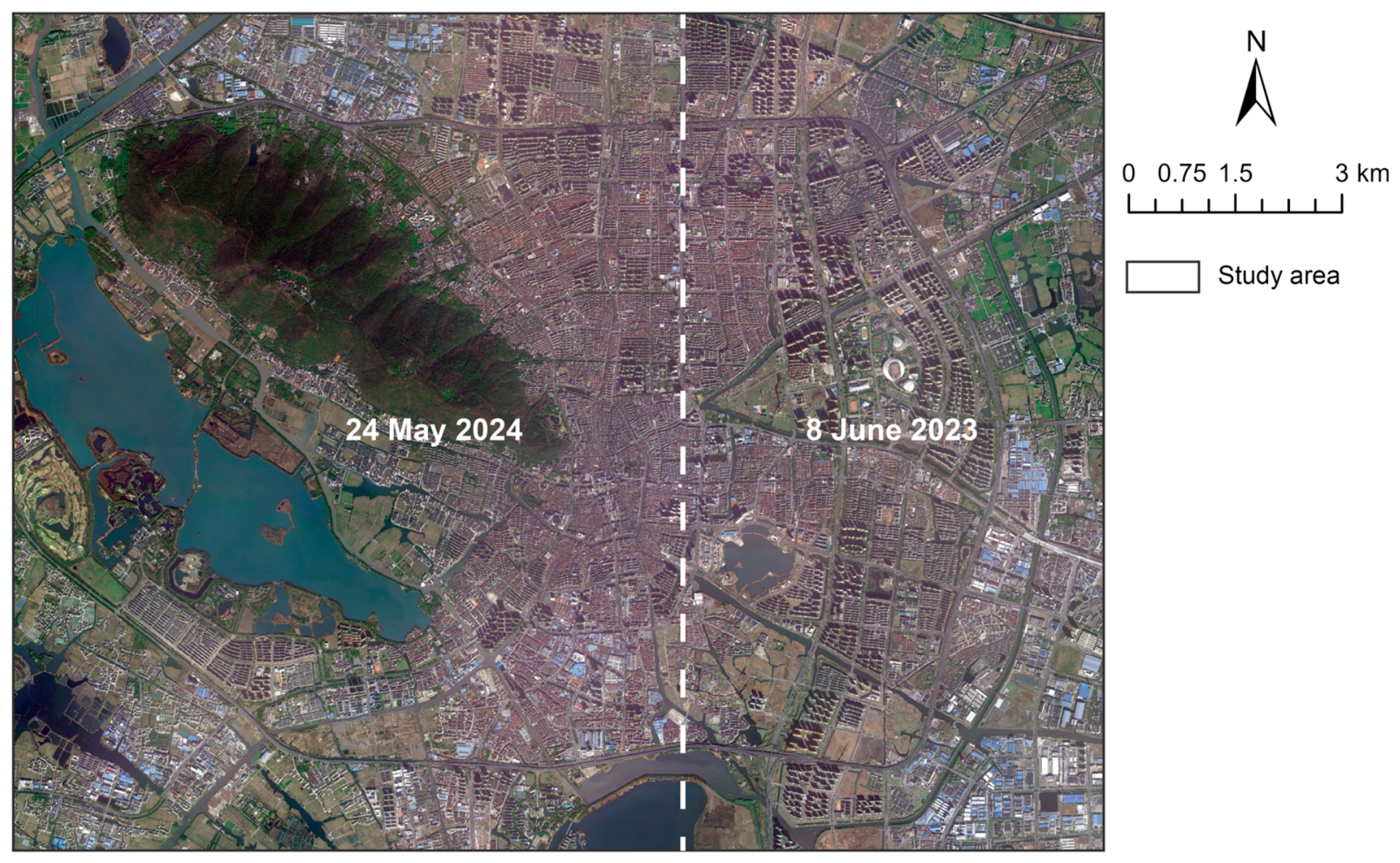
Table A1.
Characteristics of the acoustic monitoring sites used for model validation.
Table A2.
CNOSSOS-EU and OpeNoise Map simulation parameters.
References
- Yang, L.; Gutierrez, D.E.; Guthrie, O.W. Systemic Health Effects of Noise Exposure. J. Toxicol. Environ. Health Part B 2024, 27, 21–54. [Google Scholar] [CrossRef] [Scilit] [PubMed]
- O’Reilly, D.; White, M.; Langenheim, N.; Alambeigi, P. The Governance of Traffic Noise Impacting Pedestrian Amenities in Melbourne Australia: A Critical Policy Review. Int. J. Environ. Res. Public Health 2024, 21, 1080. [Google Scholar] [CrossRef] [Scilit] [PubMed]
- Van Renterghem, T.; Botteldooren, D. View on Outdoor Vegetation Reduces Noise Annoyance for Dwellers near Busy Roads. Landsc. Urban Plan. 2016, 148, 203–215. [Google Scholar] [CrossRef] [Scilit]
- Dzhambov, A.M.; Lercher, P. Road Traffic Noise Exposure and Depression/Anxiety: An Updated Systematic Review and Meta-Analysis. Int. J. Environ. Res. Public Health 2019, 16, 4134. [Google Scholar] [CrossRef] [Scilit] [PubMed]
- Gulliver, J.; Morley, D.; Vienneau, D.; Fabbri, F.; Bell, M.; Goodman, P.; Beevers, S.; Dajnak, D.; J Kelly, F.; Fecht, D. Development of an Open-Source Road Traffic Noise Model for Exposure Assessment. Environ. Model. Softw. 2015, 74, 183–193. [Google Scholar] [CrossRef] [Scilit]
- Cai, M.; Lan, Z.; Zhang, Z.; Wang, H. Evaluation of Road Traffic Noise Exposure Based on High-Resolution Population Distribution and Grid-Level Noise Data. Build. Environ. 2019, 147, 211–220. [Google Scholar] [CrossRef] [Scilit]
- Guski, R.; Schreckenberg, D.; Schuemer, R. WHO Environmental Noise Guidelines for the European Region: A Systematic Review on Environmental Noise and Annoyance. Int. J. Environ. Res. Public Health 2017, 14, 1539. [Google Scholar] [CrossRef] [Scilit] [PubMed]
- Evans, G.W.; Hygge, S.; Bullinger, M. Chronic Noise and Psychological Stress. Psychol. Sci. 1995, 6, 333–338. [Google Scholar] [CrossRef] [Scilit]
- Basner, M.; Babisch, W.; Davis, A.; Brink, M.; Clark, C.; Janssen, S.; Stansfeld, S. Auditory and Non-Auditory Effects of Noise on Health. Lancet 2014, 383, 1325–1332. [Google Scholar] [CrossRef] [Scilit] [PubMed]
- Van Kempen, E.; Casas, M.; Pershagen, G.; Foraster, M. WHO Environmental Noise Guidelines for the European Region: A Systematic Review on Environmental Noise and Cardiovascular and Metabolic Effects: A Summary. Int. J. Environ. Res. Public Health 2018, 15, 379. [Google Scholar] [CrossRef] [Scilit] [PubMed]
- Hahad, O.; Kuntic, M.; Al-Kindi, S.; Kuntic, I.; Gilan, D.; Petrowski, K.; Daiber, A.; Münzel, T. Noise and Mental Health: Evidence, Mechanisms, and Consequences. J. Expo. Sci. Environ. Epidemiol. 2025, 35, 16–23. [Google Scholar] [CrossRef] [Scilit] [PubMed]
- Murphy, E.; King, E.A. Strategic Environmental Noise Mapping: Methodological Issues Concerning the Implementation of the EU Environmental Noise Directive and Their Policy Implications. Environ. Int. 2010, 36, 290–298. [Google Scholar] [CrossRef] [Scilit] [PubMed]
- Kephalopoulos, S.; Paviotti, M.; Anfosso-Lédée, F. Common Noise Assessment Methods in Europe (CNOSSOS-EU); Publications Office of the European Union: Luxembourg, 2012. [Google Scholar]
- Salomons, E.M.; Berghauser Pont, M. Urban Traffic Noise and the Relation to Urban Density, Form, and Traffic Elasticity. Landsc. Urban Plan. 2012, 108, 2–16. [Google Scholar] [CrossRef] [Scilit]
- Can, A.; Aumond, P. Estimation of Road Traffic Noise Emissions: The Influence of Speed and Acceleration. Transp. Res. Part D Transp. Environ. 2018, 58, 155–171. [Google Scholar] [CrossRef] [Scilit]
- Kang, J. Sound Propagation in Street Canyons: Comparison between Diffusely and Geometrically Reflecting Boundaries. J. Acoust. Soc. Am. 2000, 107, 1394–1404. [Google Scholar] [CrossRef] [Scilit] [PubMed]
- Wang, B.; Kang, J. Effects of Urban Morphology on the Traffic Noise Distribution through Noise Mapping: A Comparative Study between UK and China. Appl. Acoust. 2011, 72, 556–568. [Google Scholar] [CrossRef] [Scilit]
- Echevarria Sanchez, G.M.; Van Renterghem, T.; Thomas, P.; Botteldooren, D. The Effect of Street Canyon Design on Traffic Noise Exposure along Roads. Build. Environ. 2016, 97, 96–110. [Google Scholar] [CrossRef] [Scilit]
- Mydlarz, C.; Salamon, J.; Bello, J.P. The Implementation of Low-Cost Urban Acoustic Monitoring Devices. Appl. Acoust. 2017, 117, 207–218. [Google Scholar] [CrossRef] [Scilit]
- Zuo, F.; Li, Y.; Johnson, S.; Johnson, J.; Varughese, S.; Copes, R.; Liu, F.; Wu, H.J.; Hou, R.; Chen, H. Temporal and Spatial Variability of Traffic-Related Noise in the City of Toronto, Canada. Sci. Total Environ. 2014, 472, 1100–1107. [Google Scholar] [CrossRef] [Scilit] [PubMed]
- Peckens, C.; Porter, C.; Rink, T. Wireless Sensor Networks for Long-Term Monitoring of Urban Noise. Sensors 2018, 18, 3161. [Google Scholar] [CrossRef] [Scilit] [PubMed]
- Carrasco, V.; Arenas, J.P.; Huijse, P.; Espejo, D.; Vargas, V.; Viveros-Muñoz, R.; Poblete, V.; Vernier, M.; Suárez, E. Application of Deep Learning to Enforce Environmental Noise Regulation in an Urban Setting. Sustainability 2023, 15, 3528. [Google Scholar] [CrossRef] [Scilit]
- Liu, Y.; Goudreau, S.; Oiamo, T.; Rainham, D.; Hatzopoulou, M.; Chen, H.; Davies, H.; Tremblay, M.; Johnson, J.; Bockstael, A.; et al. Comparison of Land Use Regression and Random Forests Models on Estimating Noise Levels in Five Canadian Cities. Environ. Pollut. 2020, 256, 113367. [Google Scholar] [CrossRef] [Scilit] [PubMed]
- Staab, J.; Schady, A.; Weigand, M.; Lakes, T.; Taubenböck, H. Predicting Traffic Noise Using Land-Use Regression—A Scalable Approach. J. Expo. Sci. Environ. Epidemiol. 2022, 32, 232–243. [Google Scholar] [CrossRef] [Scilit] [PubMed]
- Torija, A.J.; Genaro, N.; Ruiz, D.P.; Ramos-Ridao, A.; Zamorano, M.; Requena, I. Priorization of Acoustic Variables: Environmental Decision Support for the Physical Characterization of Urban Sound Environments. Build. Environ. 2010, 45, 1477–1489. [Google Scholar] [CrossRef] [Scilit]
- Kephalopoulos, S.; Paviotti, M.; Anfosso-Lédée, F.; Van Maercke, D.; Shilton, S.; Jones, N. Advances in the Development of Common Noise Assessment Methods in Europe: The CNOSSOS-EU Framework for Strategic Environmental Noise Mapping. Sci. Total Environ. 2014, 482–483, 400–410. [Google Scholar] [CrossRef] [Scilit] [PubMed]
- Aumond, P.; Can, A.; Mallet, V.; Gauvreau, B.; Guillaume, G. Global Sensitivity Analysis for Road Traffic Noise Modelling. Appl. Acoust. 2021, 176, 107899. [Google Scholar] [CrossRef] [Scilit]
- Morley, D.W.; de Hoogh, K.; Fecht, D.; Fabbri, F.; Bell, M.; Goodman, P.S.; Elliott, P.; Hodgson, S.; Hansell, A.L.; Gulliver, J. International Scale Implementation of the CNOSSOS-EU Road Traffic Noise Prediction Model for Epidemiological Studies. Environ. Pollut. 2015, 206, 332–341. [Google Scholar] [CrossRef] [Scilit] [PubMed]
- Bocher, E.; Guillaume, G.; Picaut, J.; Petit, G.; Fortin, N. NoiseModelling: An Open Source GIS Based Tool to Produce Environmental Noise Maps. ISPRS Int. J. Geo-Inf. 2019, 8, 130. [Google Scholar] [CrossRef] [Scilit]
- Baclet, S.; Khoshkhah, K.; Pourmoradnasseri, M.; Rumpler, R.; Hadachi, A. Near-Real-Time Dynamic Noise Mapping and Exposure Assessment Using Calibrated Microscopic Traffic Simulations. Transp. Res. Part D Transp. Environ. 2023, 124, 103922. [Google Scholar] [CrossRef] [Scilit]
- Antoniou, C.; Balakrishna, R.; Koutsopoulos, H.N. A Synthesis of Emerging Data Collection Technologies and Their Impact on Traffic Management Applications. Eur. Transp. Res. Rev. 2011, 3, 139–148. [Google Scholar] [CrossRef] [Scilit]
- Cai, D.; Chen, K.; Lin, Z.; Li, D.; Zhou, T.; Leung, M.-F. JointSTNet: Joint Pre-Training for Spatial-Temporal Traffic Forecasting. IEEE Trans. Consum. Electron. 2025, 71, 6239–6252. [Google Scholar] [CrossRef] [Scilit]
- Toole, J.L.; Colak, S.; Sturt, B.; Alexander, L.P.; Evsukoff, A.; González, M.C. The Path Most Traveled: Travel Demand Estimation Using Big Data Resources. Transp. Res. Part C Emerg. Technol. 2015, 58, 162–177. [Google Scholar] [CrossRef] [Scilit]
- Mahajan, V.; Kuehnel, N.; Intzevidou, A.; Cantelmo, G.; Moeckel, R.; Antoniou, C. Data to the People: A Review of Public and Proprietary Data for Transport Models. Transp. Rev. 2022, 42, 415–440. [Google Scholar] [CrossRef] [Scilit]
- Morley, D.W.; Gulliver, J. Methods to Improve Traffic Flow and Noise Exposure Estimation on Minor Roads. Environ. Pollut. 2016, 216, 746–754. [Google Scholar] [CrossRef] [Scilit] [PubMed]
- Fisser, H.; Khorsandi, E.; Wegmann, M.; Baier, F. Detecting Moving Trucks on Roads Using Sentinel-2 Data. Remote Sens. 2022, 14, 1595. [Google Scholar] [CrossRef] [Scilit]
- Eikvil, L.; Aurdal, L.; Koren, H. Classification-Based Vehicle Detection in High-Resolution Satellite Images. ISPRS J. Photogramm. Remote Sens. 2009, 64, 65–72. [Google Scholar] [CrossRef] [Scilit]
- Kaack, L.H.; Chen, G.H.; Morgan, M.G. Truck Traffic Monitoring with Satellite Images. In Proceedings of the 2nd ACM SIGCAS Conference on Computing and Sustainable Societies; Association for Computing Machinery: New York, NY, USA, 2019; pp. 155–164. [Google Scholar]
- Reksten, J.H.; Salberg, A.-B. Estimating Traffic in Urban Areas from Very-High Resolution Aerial Images. Int. J. Remote Sens. 2021, 42, 865–883. [Google Scholar] [CrossRef] [Scilit]
- Razakarivony, S.; Jurie, F. Vehicle Detection in Aerial Imagery: A Small Target Detection Benchmark. J. Vis. Commun. Image Represent. 2016, 34, 187–203. [Google Scholar] [CrossRef] [Scilit]
- Wang, C.-Y.; Bochkovskiy, A.; Liao, H.-Y.M. YOLOv7: Trainable Bag-of-Freebies Sets New State-of-the-Art for Real-Time Object Detectors. In Proceedings of the 2023 IEEE/CVF Conference on Computer Vision and Pattern Recognition (CVPR), Vancouver, BC, Canada, 18–22 June 2023; pp. 7464–7475. [Google Scholar]
- Sheehan, A.; Beddows, A.; Green, D.C.; Beevers, S. City Scale Traffic Monitoring Using WorldView Satellite Imagery and Deep Learning: A Case Study of Barcelona. Remote Sens. 2023, 15, 5709. [Google Scholar] [CrossRef] [Scilit]
- Cassidy, M.J.; Coifman, B. Relation Among Average Speed, Flow, and Density and Analogous Relation Between Density and Occupancy. Transp. Res. Rec. 1997, 1591, 1–6. [Google Scholar] [CrossRef] [Scilit]
- Ganji, A.; Zhang, M.; Hatzopoulou, M. Traffic Volume Prediction Using Aerial Imagery and Sparse Data from Road Counts. Transp. Res. Part C Emerg. Technol. 2022, 141, 103739. [Google Scholar] [CrossRef] [Scilit]
- Gao, F.; Li, B.; Xu, Q.; Zhong, C. Moving Vehicle Information Extraction from Single-Pass WorldView-2 Imagery Based on ERGAS-SNS Analysis. Remote Sens. 2014, 6, 6500–6523. [Google Scholar] [CrossRef] [Scilit]
- Xu, X.; Ge, Y.; Wang, W.; Lei, X.; Kan, H.; Cai, J. Application of Land Use Regression to Map Environmental Noise in Shanghai, China. Environ. Int. 2022, 161, 107111. [Google Scholar] [CrossRef] [Scilit] [PubMed]
- Espadaler-Clapés, J.; Barmpounakis, E.; Geroliminis, N. Traffic Congestion and Noise Emissions with Detailed Vehicle Trajectories from UAVs. Transp. Res. Part D Transp. Environ. 2023, 121, 103822. [Google Scholar] [CrossRef] [Scilit]
- Aszkowski, P.; Ptak, B.; Kraft, M.; Pieczyński, D.; Drapikowski, P. Deepness: Deep Neural Remote Sensing Plugin for QGIS. SoftwareX 2023, 23, 101495. [Google Scholar] [CrossRef] [Scilit]
- Yang, M.Y.; Liao, W.; Li, X.; Cao, Y.; Rosenhahn, B. Vehicle Detection in Aerial Images. Photogramm. Eng. Remote Sens. 2019, 85, 297–304. [Google Scholar] [CrossRef] [Scilit]
- Fogola, J.; Grasso, D.; Masera, S.; Scordino, P. OpeNoise: A Free and Open Source Project for Environmental Noise Assessment. In Proceedings of the 10th Convention of the European Acoustics Association Forum Acusticum 2023; European Acoustics Association: Turin, Italy, 2024; pp. 67–73. [Google Scholar]
- Shepard, D. A Two-Dimensional Interpolation Function for Irregularly-Spaced Data. In Proceedings of the 1968 23rd ACM National Conference; Association for Computing Machinery: New York, NY, USA, 1968; pp. 517–524. [Google Scholar]
- GB 3096-2008; Environmental Quality Standard for Noise. Standards Press of China: Beijing, China, 2008.
- Salehi, B.; Zhang, Y.; Zhong, M. Automatic Moving Vehicles Information Extraction From Single-Pass WorldView-2 Imagery. IEEE J. Sel. Top. Appl. Earth Obs. Remote Sens. 2012, 5, 135–145. [Google Scholar] [CrossRef] [Scilit]
- Leitloff, J.; Rosenbaum, D.; Kurz, F.; Meynberg, O.; Reinartz, P. An Operational System for Estimating Road Traffic Information from Aerial Images. Remote Sens. 2014, 6, 11315–11341. [Google Scholar] [CrossRef] [Scilit]
- ISO 9613-1:1993; Acoustics—Attenuation of Sound During Propagation Outdoors—Part 1: Calculation of the Absorption of Sound by the Atmosphere. International Organization for Standardization: Geneva, Switzerland, 1993.
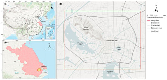
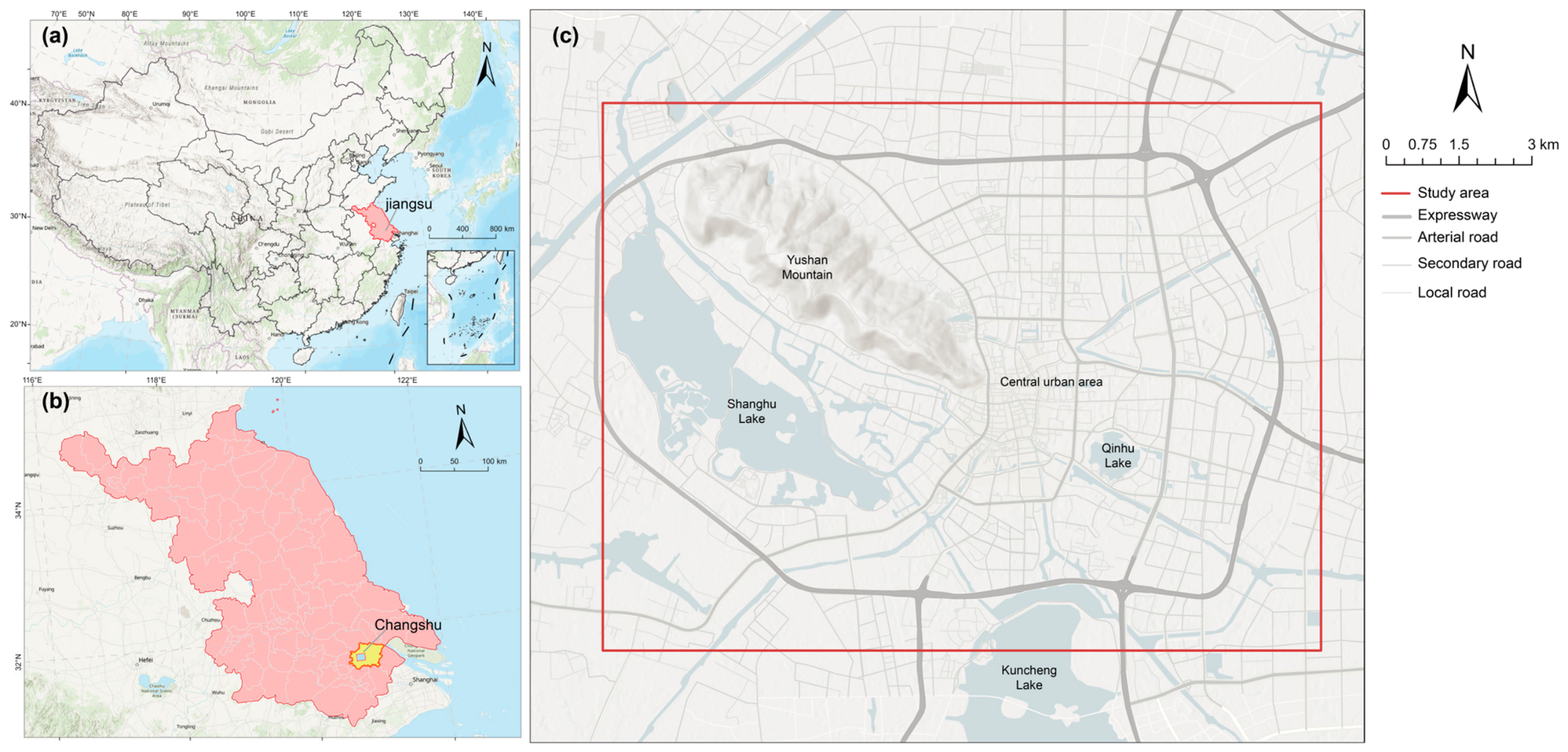
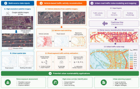
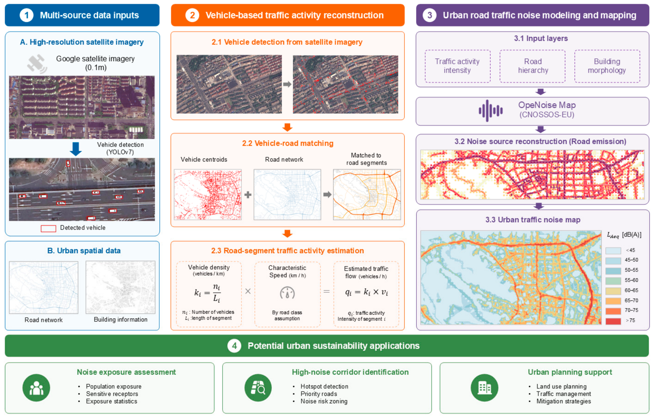
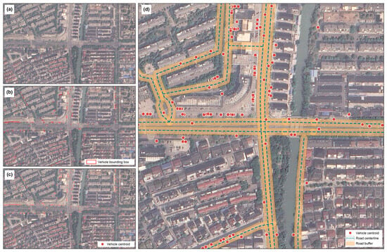
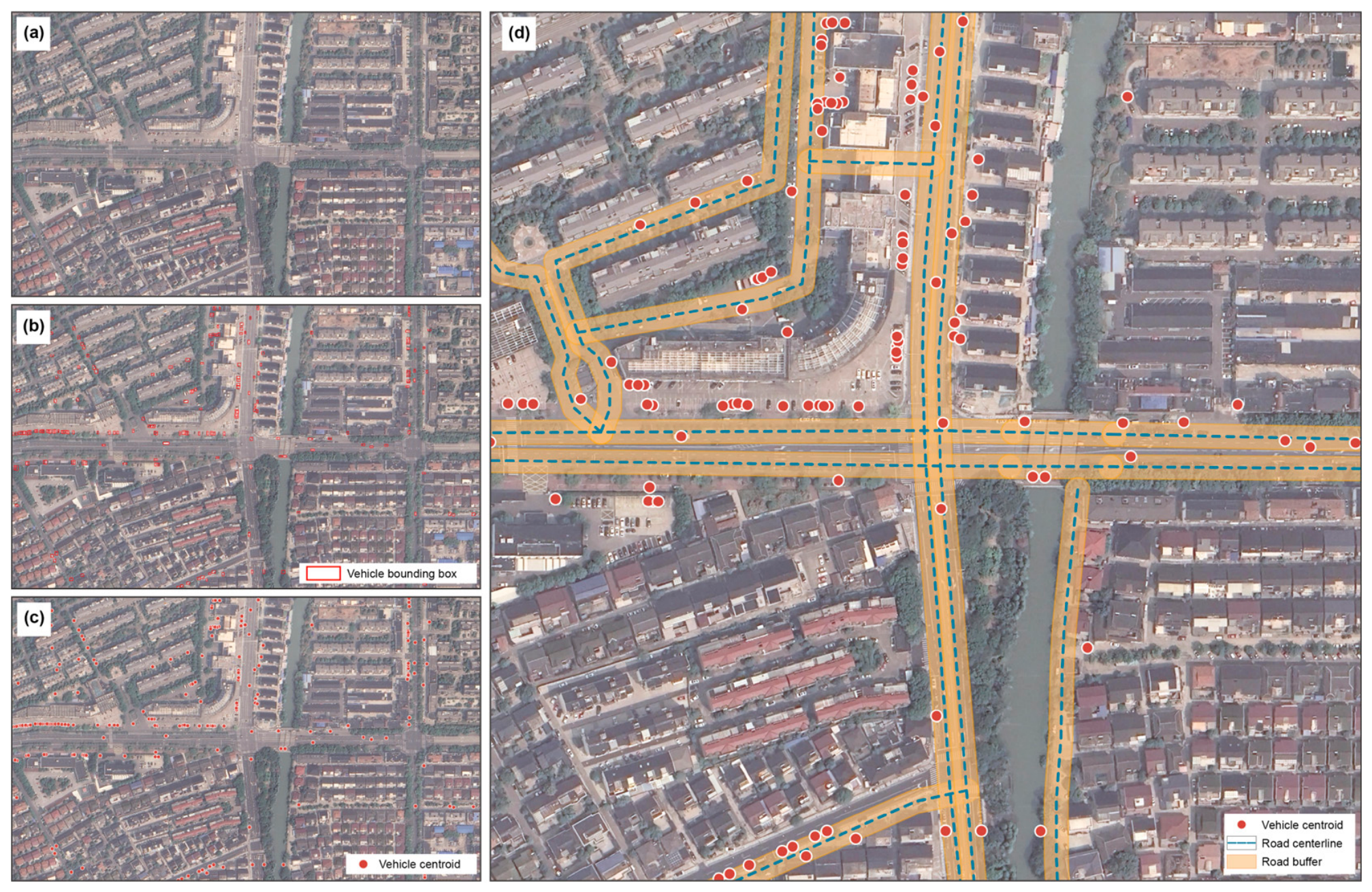
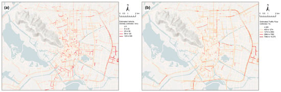
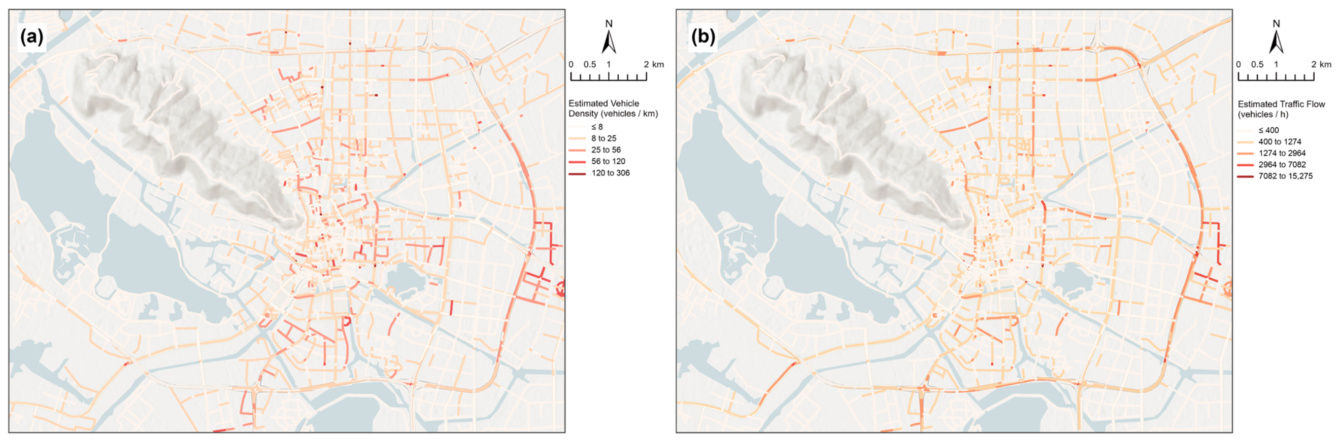
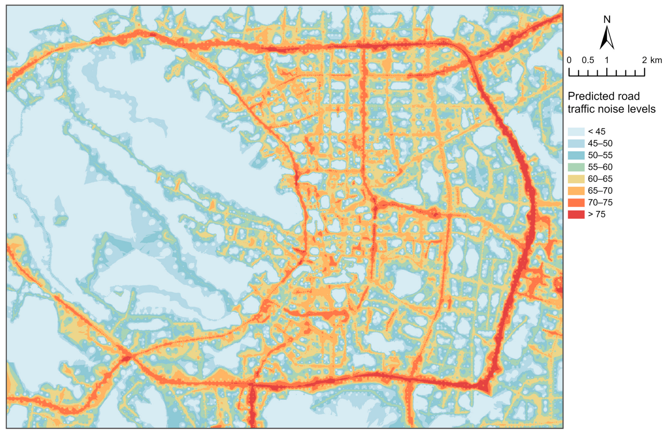
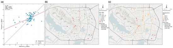
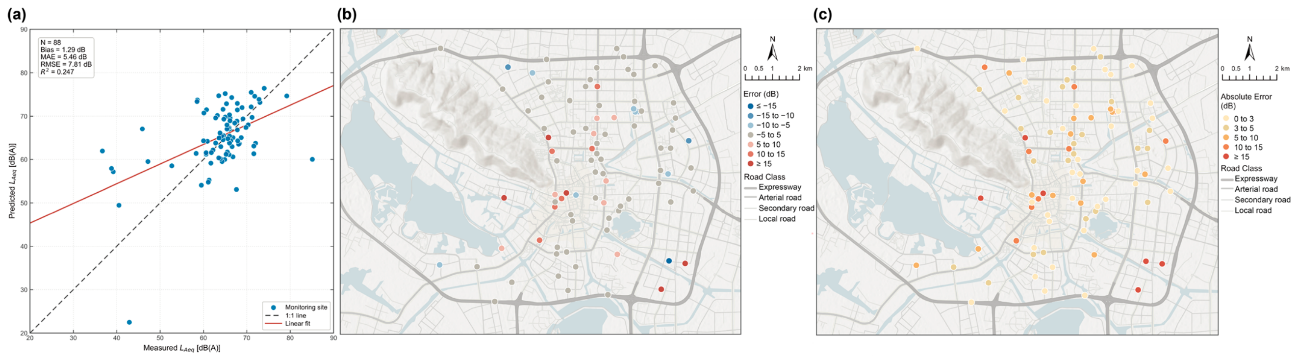

Disclaimer/Publisher’s Note: The statements, opinions and data contained in all publications are solely those of the individual author(s) and contributor(s) and not of MDPI and/or the editor(s). MDPI and/or the editor(s) disclaim responsibility for any injury to people or property resulting from any ideas, methods, instructions or products referred to in the content. |
© 2026 by the authors. Licensee MDPI, Basel, Switzerland. This article is an open access article distributed under the terms and conditions of the Creative Commons Attribution (CC BY) license.