


Abstract
Peripheral-station and representative-year weather files can misrepresent urban thermal conditions. This study quantifies how reference, weather construction, and temporal definition condition urban heat-island (UHI) effects on residential performance in Turin to support proper sustainable climate design studies. Seven-station observations (2014–2023) underpin processed actual meteorological years (AMYs), calendar-hour-average years (AvMYs), and regenerated typical meteorological years (TMYs). We introduce a new method, the Controlled Urban Weather Forcing (CUWF), which substitutes declared psychrometric variables within a common Caselle background; full-field and al, it is correct. Since polito is also the affiliation of mine (Chiesa), do we also need my email here, or is it ternative-reference cases test the boundaries. A DOE–TABULA apartment archetype, with two envelope states and three operating modes, was evaluated through 452 annual EnergyPlus simulations. Across ten matched AMYs, urban forcing increased useful sensible cooling by 2.8–12.3% and reduced heating by 5.3–25.8%. Original-envelope full-field Consolata relative to Caselle changed heating by −13.7% and cooling by +17.8%. TMY needs remained near AvMY values, but original-envelope cooling peaks increased by 38.7% at Caselle and 57.5% at Consolata. The AMYs contained 26 Caselle-defined persistent hot events, whereas the AvMY contained none under the same threshold. Rank-based, leave-one-year-out, daily aggregation, and lag analyses retained response directions but confirmed that degree-hours, dynamic loads, and overheating exposure are not interchangeable. Climate-resilient design should therefore specify the reference, weather representation, envelope, and control mechanism rather than treat UHI as a uniform offset, thereby properly supporting building and urban sustainable design and policy-correlated aspects.
1. Introduction
An urban heat island (UHI) is spatially and temporally variable, and its inferred magnitude depends on the reference, local surface and morphology, station exposure, weather conditions, season, and hour [1,2,3]. Urban–reference humidity contrasts require comparable care, because relative humidity responds directly to temperature. An urban dry island (UDI) is more physically interpretable when expressed in terms of a temperature-independent moisture metric, such as the humidity ratio or vapour pressure [4]. UHI is therefore not a unique city constant. This matters for buildings because warmer urban air can reduce winter heating needs, increase summer cooling needs, and alter the outdoor heat sink available to passive or hybrid cooling [5,6]. In a mixed station network, the measured contrast should be interpreted as an exposure-inclusive station-air difference rather than as a pure canopy-layer or morphology effect unless source areas and measurement heights are demonstrably comparable [7,8].
Several methods introduce urban climate into building-performance simulation, including direct observations, fixed-offset or empirical morphing, simplified urban-canopy weather generators, mesoscale or microscale coupling, and spatial or statistical localisation [9,10]. Direct measurements preserve site-specific temporal behaviour, but their use is limited by station siting, missing variables, data processing, and the frequent need to combine urban psychrometric observations with radiation, wind, and pressure data from other sources. Urban meteorological generators and localised station assignments can represent more weather fields or spatial contexts, while comparisons with climate-station and conventional EPW data show that the selected weather source can materially affect simulated building outcomes [11,12,13]. Synthetic and localised methods can therefore support morphology or intervention studies, but their conclusions depend on calibration, representative inputs, and explicit field provenance. The weather intervention and its uncertainty must be stated.
Observational and simulation studies have established that urban overheating can reduce heating requirements while increasing cooling needs, peak demand, and thermal exposure. Large-scale empirical building data show simultaneous increases in cooling and reductions in heating associated with urban overheating [14], while Mediterranean and Italian residential studies using urban and non-urban weather have demonstrated that reference weather and absolute-moisture conditions can materially affect sensible and latent loads [15,16]. Long records and multi-station networks have also been combined with dynamic simulation in Beijing, Nanjing, San Francisco, Rome, and other cities [17,18,19,20,21,22]. Recent studies have examined seasonal and diurnal effects in residential buildings, interactions between UHI and building or operational parameters, and nighttime cooling during heat waves [23,24,25]. A Turin station dataset and its EPW/TMY-generation (Typical Meteorological Year) procedure were published previously [26]. Turin UHI and UDI, including sensitivity to northern and southern reference contexts, have also been characterised [27], and representative Turin urban and non-urban sites have been investigated using temperature-difference matrices and principal-component analysis [28]. The present study does not claim novelty for those source-data or TMY procedures. Its contribution is to construct and evaluate calendar-hour AvMYs (average Meteorological Year), define a controlled urban weather forcing method, propagate alternative-reference and full-field weather choices through a common residential archetype, and align climate indicators with dynamic building-response mechanisms across AMY (Actual Meteorological Year), AvMY, and TMY representations.
This temporal correspondence is central to the present study. Urban heat can persist beyond daytime forcing due to heat storage in urban materials, whereas observed indoor temperatures respond more slowly than outdoor air temperatures and can retain heat for multiple days [29,30]. Mechanically cooled buildings respond to heat gains accumulated throughout the cooling season, whereas night ventilation depends directly on the availability of cooler outdoor air during the ventilation period. Previous research has demonstrated the importance of UHI, neighbourhood climate, wind shielding, and urban mitigation for ventilative cooling [31,32,33,34,35,36]. Building on this evidence, the present analysis examines whether UHI summaries defined over different time intervals yield different interpretations when urban sites, source years, reference stations, envelope states, operating modes, temporal aggregation, and response lag are evaluated within a common controlled-weather framework.
Weather-year construction introduces an additional methodological time dimension, consistent with the need to treat climate inputs as time-dependent design information rather than immutable site constants [37]. A standard TMY is assembled from representative source months selected from a multiyear record, whereas an AMY preserves a source-year sequence [38]. The AvMY considered here differs from both in that the corresponding calendar hours are averaged across source years, thereby smoothing the chronology and joint extremes. The length and recency of the source record affect representative-weather construction [39], and comparisons using DOE reference buildings show that typical-year simulations may approximate central annual outcomes without reproducing the range of historical years [40]. Typical or average-pattern weather files may therefore approximate central annual loads while underrepresenting interannual variability, peaks, persistence, and threshold events [41]. Accordingly, AvMY is evaluated as a mean-pattern representation; regenerated station-specific TMYs are evaluated as selected-month design representations; and matched AMYs provide evidence of variability and sign persistence.
1.1. Research Questions
The study addresses one primary research question and three supporting questions:
- Primary question: To what extent, and through which response-relevant time scales, do measured urban station-air conditions translate into useful thermal needs, overheating exposure, and night-ventilation performance in a controlled residential archetype?
- Supporting question 1: How do the magnitude and temporal signature of station-air UHI and humidity-ratio UDI vary among the four Turin urban stations, and how sensitive are the inferred climate and building effects to the non-urban reference?
- Supporting question 2: What characteristics are preserved or suppressed when the 2014–2023 station record is represented as chronological AMYs, calendar-hour AvMYs, or selected-month TMYs, and how do those representations affect annual, peak, and persistent-heat indicators?
- Supporting question 3: How do reference choice, controlled versus processed full-field weather, envelope state, operating mode, temporal aggregation, and lag affect the relationship between UHI, outdoor degree-hours, and dynamic building responses?
To answer these questions, this paper introduces a new approach for defining and computing the controlled urban weather forcing (CUWF) at a given location.
1.2. Study Objectives and Contribution
The general objective is to quantify and interpret how measured urban station-air conditions, represented through traceable weather products and the newly defined CUWF method, alter the thermal performance of a controlled residential archetype in Turin.
The specific objectives are to (i) characterise station-specific UHI, humidity-ratio UDI, and outdoor degree-hour signatures on matched temporal support; (ii) determine how reference selection and weather-field provenance affect the inferred urban building response; (iii) compare the roles of chronological AMY, mean-pattern AvMY, and selected-month TMY representations; (iv) evaluate whether envelope state and conditioned, sealed free-running, or night-ventilated operation change the magnitude or temporal alignment of the response; and (v) test the robustness of the principal annual relationships through rank-based, leave-one-year-out, aggregated, and exploratory lag analyses.
The principal contribution is not the previously published Turin station archive or its EPW/TMY-generation workflow [26], but the response-relevant experiment built upon it: a named CUWF method with declared retained fields, matched AMY and AvMY building comparisons, complementary alternative-reference and processed full-field sensitivities, a regenerated TMY benchmark, and an explicit distinction between mathematically coupled climate indicators and dynamic building responses. This combination provides a reproducible basis for weather-informed retrofit, conditioning, and passive-cooling decisions without treating UHI as a uniform offset.
The analysis is limited to useful thermal energy needs, Ideal Loads peaks, and modelled thermal exposure; delivered energy, utility consumption, costs, carbon emissions, health outcomes, and energy-performance certification are not evaluated. Heating reductions and cooling increases are therefore reported as separate seasonal design consequences rather than combined as a net annual benefit.
2. Materials and Methods
2.1. Study Design
The analysis comprised five connected stages. First, the seven-station 2014–2023 record was screened for station suitability, quality, common temporal support, and urban/reference roles. Second, the processed station observations were organised as chronological AMYs, calendar-hour AvMYs, and regenerated selected-month TMYs with explicit field lineage. Third, CUWF files were constructed by substituting declared psychrometric variables within a common Caselle background, while alternative-reference and processed full-field cases were prepared as separate sensitivities. Fourth, the identical DOE–TABULA building cases were simulated under the declared weather, envelope, and operating-mode combinations. Fifth, urban-minus-reference climate and building responses were compared at hourly, aggregated, annual, and decadal-summary scales, including persistence, robustness, and lag checks. These stages distinguish measured station contrasts, weather-year representation, controlled attribution, building response, and mechanism-specific interpretation.
Figure 1 summarises the station context and analytical design.
Figure 1.
Station context and analytical workflow: (a) station positions from the dated ARPA configuration records, with a star denoting the primary peripheral reference proxy, plus symbols denoting alternative non-urban references, and circles denoting the four urban cases; and (b) the five-stage sequence from station-role and quality assessment, through AMY/AvMY/TMY weather construction and the controlled urban weather forcing method, to EnergyPlus simulation and response-specific comparison. The processed full-field sensitivity is shown outside the CUWF boundary. Symbols indicate analytical roles rather than LCZ assignments.
2.2. Source Weather Records and Station Roles
The source archive comprised 70 processed, measurement-derived EPWs representing seven stations and ten source-weather years from 2014 to 2023. These files preserve the processed station-year sequences used to construct the AMY, AvMY, TMY, and controlled products described in Section 2.3 and Section 2.4; they are not assumed to contain only direct measurements or to satisfy every executable-field gate without the declared downstream preparation.
Station suitability was assessed from (i) availability within the common 2014–2023 study period; (ii) availability and usable support for dry-bulb temperature and relative humidity; (iii) the geographical role required for an urban or plausible peripheral/background comparison; (iv) a dated ARPA station configuration and coordinates; and (v) sufficient matched records for the intended analysis. Temperature deployment, elevation, land-cover context, detected invalid values, and known lineage limitations were treated as interpretation qualifications rather than as retrospective homogenisation variables (Table 1 and Table A7).
Table 1.
Station metadata, temperature-sensor deployment, and analytical role.
Four stations were selected as urban cases: Via della Consolata, Giardini Reali, Alenia, and Reiss Romoli. Caselle was used as the primary peripheral/background proxy because it provides the complete common non-psychrometric control required by CUWF; at 285 m elevation, it is a peripheral airport setting rather than undisturbed rural land. Bauducchi, at 226 m and within a predominantly agricultural 500 m context, was used both as an alternative climate reference and as a controlled thermohygrometric building baseline. Venaria La Mandria was retained as an additional climate-reference sensitivity, but its 2019 record was excluded because the temperature/humidity lineage and header are corrupted. Multiple plausible reference definitions, including airport references, can produce materially different UHI estimates [42].
Meteoidro API records [43]. Surrounding land-cover context was quantified at radii of 100 and 500 m using Regione Piemonte Land Cover Piemonte 2021 [44]. These fractions provide contextual information and were not used to assign LCZ classes or to correct measurements for height. Table 1 summarises the station metadata and analytical roles; detailed land-cover fractions are reported in Table A6, and the post-generation quality and completeness audit is reported in Table A7.
2.3. Controlled Urban Weather Forcing and Complementary Weather Sensitivities
The station records described in Section 2.2 were checked for structural coverage, ordered timestamps, duplicate calendar keys, physically invalid values, and completeness before their assembly as executable weather products. The audit confirmed 8760 ordered records in each of the 70 processed AMYs. Three invalid urban dry-bulb records (0.000856% of 350,400 urban records) were linearly interpolated between the nearest valid same-station hours for executable matched-year forcing; 70 zero or invalid urban relative-humidity records (0.01998%) were replaced by matched-hour Caselle relative humidity; and 185 Caselle pressure records reported as 600 hPa (0.21119% of Caselle records) were interpolated before conversion to pascals. Table A7 distinguishes these downstream executable corrections from upstream processing whose per-record measured, filled, or recomputed status cannot be reconstructed. Controlled AvMY forcings and retained-field rules are recorded in UHI_FORCING_EPW_MANIFEST.json; matched-year AMY forcings and executable corrections are recorded in AMY_YEARLY_FORCING_MANIFEST.json; and complementary full-field, TMY, and alternative-reference inputs are recorded in REVISION_WEATHER_MANIFEST.json. The three machine-readable manifests are publicly available at Zenodo at https://doi.org/10.5281/zenodo.22249269 (accessed on 13 September 2026), and Table A8 provides their human-readable field-provenance summary.
The controlled urban weather forcing (CUWF) method is defined here as a paired EPW construction in which predeclared urban psychrometric fields replace the corresponding reference fields, dependent psychrometric variables are recomputed, and the reference location, calendar, radiation, long-wave radiation, wind, pressure, and all remaining EPW fields are held fixed. Two CUWF AvMY variants were constructed:
- TEMP_ONLY: urban dry-bulb temperature replaces Caselle dry-bulb temperature while Caselle dew point is retained as a fixed absolute-moisture proxy; relative humidity is recomputed psychrometrically.
- TEMP_RH: urban dry-bulb temperature and relative humidity replace the Caselle values; dew point is recomputed psychrometrically.
Both AvMY variants retain the declared Caselle control fields. For each source-year AMY, only the joint temperature–relative-humidity (TEMP_RH) substitution was applied; TEMP_ONLY was evaluated only in the AvMY sensitivity analysis. The 50 matched-year forcings comprise ten source years, each represented by one Caselle control and four urban TEMP_RH files, and therefore evaluate chronological thermohygrometric forcing. Paired TEMP_ONLY and TEMP_RH AvMY cases distinguish moisture-field specification. A controlled Bauducchi AvMY baseline was additionally generated by inserting Bauducchi dry-bulb temperature and relative humidity into the same Caselle non-psychrometric context, permitting reference propagation without confounding the comparison by full-field differences.
A processed full-field Consolata AvMY was simulated as a complementary sensitivity outside CUWF. It uses the same Consolata dry-bulb temperature, relative humidity, and recomputed dew point as the controlled Consolata TEMP_RH case, but releases the common-background constraint by retaining the processed Consolata location and available station-specific or derived radiation, wind, pressure, long-wave, and remaining fields. This comparison tests the collective consequence of releasing the Caselle non-psychrometric background; it does not decompose individual fields or represent a wholly measured urban microclimate. The mutually coupled nature of urban temperature, humidity, radiation, wind, and other meteorological fields is therefore treated as a claim boundary rather than ignored [11,45].
All simulations use a standardised non-leap 2017 schedule calendar, UTC+1 standard time, no daylight-saving time, and no holidays or special days. A filename year identifies the source thermohygrometric sequence, not a reconstructed historical weekday calendar. AMY, AvMY, and regenerated TMY construction are used; Section 2.8 defines the corresponding simulation families.
2.4. Measurement-Derived EPW Generation
The production of the 70 processed, measurement-derived station-year EPWs followed the previously published Turin data workflow [26]. For each station and year, the ARPA Piemonte variable-specific CSV records were acquired, timestamps and units were standardised, and air temperature, relative humidity, wind speed and direction, atmospheric pressure, and global solar irradiation were merged on a common hourly index. Missing or invalid observations were treated using the variable-dependent procedures reported with the source dataset: short gaps were interpolated, while wind and solar gaps could use information from correlated stations. EPW-required variables that were not directly observed were then derived. In particular, global horizontal irradiation was partitioned into diffuse horizontal and direct normal components using the PREDYCE implementation of the Boland approach, and horizontal infrared radiation and psychrometric fields were calculated as required by the compiler. Station metadata and the completed hourly records were written using custom Python (v3.13.6) routines to the EPW structure used by EnergyPlus (v26.1.0). These published source-data and EPW-generation procedures are inputs to, rather than the novelty claimed for, the present CUWF and building-response analysis. The additional corrections required for the present executable forcing set are reported separately in Section 2.3 and Table A7 and Table A8.
Each processed station-year sequence is termed an AMY in this study and preserves the temporal ordering of its source year after the declared processing. A station AvMY was generated by independently averaging corresponding non-leap calendar hours across the ten AMYs to obtain an 8760-record mean-pattern year. The AvMY is therefore neither a chronological observed year nor a TMY and can attenuate persistence, covariance, and extremes. For the representative-year benchmark, Caselle and Consolata TMYs were regenerated from all ten 2014–2023 AMYs using a declared implementation of ISO 15927-4. For each calendar month, daily mean dry-bulb temperature, global horizontal irradiation, and relative humidity were ranked independently by their Finkelstein–Schafer statistics; the three lowest equal-weight rank sums were retained, and the candidate whose monthly mean wind speed was nearest the ten-year monthly mean was selected. Ties at the three-candidate cutoff were resolved by the lower summed unrounded Finkelstein–Schafer statistic and then the earlier year. Selected months were joined using an additive cubic-Hermite correction over the last eight and first eight records at each of the 12 seams, after which dew point was recomputed; pressure repairs and all selected month/year lineages are reported in the complementary weather-input manifest (REVISION_WEATHER_MANIFEST.json; Table A8). The previously published TMY candidates were audited but not simulated because their traceable source-month lineage covered only 2014–2016; they were retained as provenance comparators. The regenerated TMYs are compared with AvMYs only through annual, seasonal, and peak KPIs, not hour by hour [38].
2.5. Climate Indicators and Temporal Definitions
The station-air UHI intensity was calculated at each matched reported hour as
where T_u and T_r are the urban and selected reference dry-bulb temperatures. Positive values indicate warmer urban-station air. No interpolation was performed solely to increase matched coverage.
I_UHI(t) = T_u(t) − T_r(t),
Because relative humidity depends on air temperature, UDI was evaluated using the humidity ratio w, expressed as grams of water vapour per kilogram of dry air. Vapour pressure e and humidity ratio were obtained from the reported dry-bulb temperature, relative humidity, and pressure using
where φ is relative humidity (%), p_ws is saturation vapour pressure, and p is atmospheric pressure. The signed humidity-ratio UDI intensity was then defined as
where positive values indicate lower urban moisture content and hence a dry-island episode; negative values indicate an urban moisture-island episode. This sign convention permits the term UDI to be retained without interpreting a relative-humidity deficit caused by warming as an independent reduction in atmospheric water content [4].
e(t) = [φ(t)/100] p_ws[T(t)]; w(t) = 1000 × 0.621945 e(t)/[p(t) − e(t)],
I_UDI,w(t) = w_r(t) − w_u(t),
For the AvMY UDI diagnostic, the humidity ratio was calculated in each matched AMY before the ten corresponding calendar-hour values were averaged. The urban and reference members used their respective dry-bulb and relative-humidity sequences with the common matched Caselle pressure retained by the controlled-weather design. This derive-first, average-second sequence avoids the psychrometric inconsistency that can arise when independently averaged AvMY dry-bulb, relative-humidity, and dew-point fields are recombined through a nonlinear relation. The averaged AvMY dew-point field was therefore not used to determine UDI.
Outdoor cooling and heating degree-hours were used as weather-derived screening indicators for comparing station contrasts with building simulations. For an hourly interval Δt = 1 h,
where T_o is the outdoor dry-bulb temperature. The bases of 24 °C for CDH and 18 °C for HDH follow the climate-indicator definition adopted in the earlier methodological framework and are distinct from the 26 °C cooling and 20 °C heating setpoints used in the EnergyPlus model. Annual urban effects are expressed as ΔCDH_24 = CDH_24,u − CDH_24,r and ΔHDH_18 = HDH_18,u − HDH_18,r. Thus, urban warming generally produces a positive cooling-degree-hour difference and a negative heating-degree-hour difference; neither quantity is a building energy need.
CDH_24 = Σ_t max[T_o(t) − 24, 0] Δt,
HDH_18 = Σ_t max [18 − T_o(t), 0] Δt,
Because UHI, CDH, and HDH are all calculated from the same urban–reference outdoor-temperature pair, their annual correlations are mathematically coupled weather-indicator consistency checks rather than independent validation. The more consequential test is whether the imposed meteorological contrast translates into a dynamic building response conditioned by storage, gains, ventilation, schedules, and control.
The cooling season was defined as 16 April–14 October, consistent with the complement of Turin’s prescribed heating period of 15 October–15 April, as set out in D.P.R. 412/1993 and subsequent modifications. The nighttime interval was 19:00–07:00 local standard time; under EPW hour-ending labels, this corresponds to hours 20–24 and 1–7 [46]. Cooling-season UHI was paired with CDH and mechanically cooled response, heating-season UHI with HDH and heating response, and cooling-night UHI with the night-ventilation response. Source-year means were equally weighted. Ninety-five per cent intervals were calculated using a fixed-seed whole-year bootstrap with 10,000 resamples. Reference sensitivity used identical common-year and matched-hour support.
Heat-event persistence was evaluated using Caselle cooling-season daily maximum temperatures across the ten AMYs. The fixed threshold was the pooled AMY 90th percentile (31.8 °C), and an event required at least three consecutive days above that threshold. The identical threshold and the duration rule were then applied to the Caselle AvMY. For each AMY event, the following-night interval comprised EPW hour-ending records 20–24 on each hot day and 1–7 on the next day; station-specific UHI means were first calculated by source year and then equally weighted across the ten years. This is a study-defined weather-persistence indicator, not a health, regulatory, or event-level building-performance threshold [29].
2.6. Building Archetype and Envelope States
The building was represented by a generic comparative DOE–TABULA hybrid archetype. Its four-storey geometry, zoning, multipliers, and approximately 15% window-to-wall ratio derive from the official DOE New2004 Midrise Apartment Version 1.4/EnergyPlus 7.2 prototype [47]. The model was converted through the official version-transition sequence and simulated with EnergyPlus 26.1.0 [48]. The former office-zone geometry was retained, while schedules, loads, infiltration, outdoor-air sizing, and the domestic-hot-water connection were converted to a residential programme aligned with EN 16798-1:2019. The model contains 24 representative occupied apartment zones and three corridors, representing 32 apartments after the retained DOE middle-floor multipliers. The conditioned floor area is 3134.59 m2, and the occupied residential area used for threshold KPIs is 2823.9579 m2. This controlled geometry is suitable for comparative sensitivity analysis, not for calibrated prediction of the Turin residential stock; Table A9 records the source, implementation, and claim boundary for each model element [49].
Envelope targets follow the Italian AB.05 apartment-block typology in the European TABULA building-typology framework for 1961–1975 and its advanced refurbishment [50,51]. The same DOE geometry, window arrangement, schedules, and represented apartment count are used in both states; TABULA supplies comparative envelope-performance targets rather than the building geometry. Massive layers are reconstructed [52,53].
The original-to-advanced component targets are 1.10 to 0.25 W m−2 K−1 for exterior walls, 1.65 to 0.23 W m−2 K−1 for the direct-roof/upper-slab proxy, 1.30 to 0.23 W m−2 K−1 for the lower-floor/cellar proxy, 4.90 to 1.70 W m−2 K−1 for windows, and 0.85 to 0.50 for the whole-window SHGC proxy.
The baseline residential programme uses 2.5 persons per representative apartment, 3.88 W m−2 lighting, and 5.38 W m−2 plug equipment. Twenty-seven ZoneInfiltration:DesignFlowRate objects use Flow/ExteriorArea at 0.000302 m3 s−1 m−2, approximately 0.284–0.296 h−1 cooling-season occupied-area-weighted mean infiltration in baseline runs. Schedules and gains are common to both envelopes. The envelope states change bundled U-value, glazing, SHGC, and reconstructed-material assumptions; their difference cannot be attributed to insulation alone. Table A5 provides the compact input register, and Table A9 distinguishes DOE, TABULA, standard, and study-defined inputs.
2.7. Operating Modes and Seasonal Controls
Space conditioning uses ZoneHVAC:IdealLoadsAirSystem; outputs are useful thermal energy needs rather than final energy or primary energy. Three cases are simulated, varying the summer season ventilation approach:
- SYS_ON: heating is available from 15 October to 15 April at a 20 °C setpoint; cooling is available from 16 April to 14 October at a 26 °C setpoint; windows remain closed.
- FREE: the same winter heating is available, summer mechanical cooling is unavailable, and windows remain closed.
- FREE_NV: the same winter heating is available, and summer mechanical cooling is unavailable, with conditional wind-and-stack window opening during the cooling season.
FREE therefore means cooling-season free-running, not a fully unconditioned year.
The FREE_NV case uses 36 ZoneVentilation:WindandStackOpenArea objects. Each apartment window is modelled as 50% operable; a 20% opening schedule, when eligible, gives a 10% effective opening relative to the total glazing. Eligibility is 19:00–07:00 in the cooling season, with heating off, indoor air temperature at least 18 °C, and T_in − T_out ≥ 3 K. Opening effectiveness and discharge coefficient are Autocalculate; façade angle follows each window, and the opening height difference is 0.60955 m. The controller represents one simplified implementation within the broader family of ventilative-cooling principles and controls [46].
The primary maximum-wind field is 40 m s−1. A 10 m s−1 closure check and a second threshold of 2.5 m s−1 were also tested. The latter was specified a priori by rounding the Caselle cooling-night site-wind 90th percentile, 2.483 m s−1, to 2.5 m s−1. The building terrain category is City; consequently, EnergyPlus applies height- and terrain-adjusted local wind velocities at each zone rather than the EPW site wind value directly.
2.8. Simulation Design and Sensitivity Analyses
The simulation matrix comprises 452 annual EnergyPlus cases: 54 AvMY cases (nine weather forcings × six building cases), 300 matched-year cases (ten years × five weather variants × six building cases), 74 deterministic physical and operational sensitivity cases, and 24 complementary cases. The latter comprise six processed full-field Consolata AvMY cases, six controlled Bauducchi-reference AvMY cases, and 12 regenerated station-specific TMY cases (Caselle and Consolata × six building cases).
The three complementary simulation families address distinct methodological questions. Controlled Consolata relative to controlled Caselle or controlled Bauducchi tests reference propagation within the common Caselle non-psychrometric context. Full-field Consolata relative to controlled Consolata tests the collective sensitivity to releasing that common background, while full-field Consolata relative to the Caselle AvMY control provides an exposure-inclusive practical contrast. Regenerated Caselle and Consolata TMYs are compared with their corresponding AvMYs only through aggregate annual, seasonal, and peak KPIs. The location-dependent full-field and TMY simulations use model copies aligned with the respective Caselle or Consolata weather location; the building physics, envelopes, schedules, and operating modes remain otherwise identical.
The opening-area, SHGC (solar heat gain coefficient), wind, gain, infiltration, and lower-floor analyses were restricted to the CONTROL_CASELLE and TEMP_ONLY_CONSOLATA AvMY forcings; they did not include TEMP_RH, the other three urban stations, the full-field case, alternative-reference case, or TMYs. The opening area was evaluated in 12 additional cases using 5%, 10%, and 20% effective opening across Caselle, Consolata, and both envelope states. The SHGC analysis combined 18 additional simulations with 18 corresponding core cases, yielding 36 comparison cells. Eight additional simulations and four corresponding core cases formed the 12-cell wind-threshold analysis. Finally, 36 one-factor simulations and 12 corresponding baselines formed a 48-cell analysis of internal gains, infiltration, and lower-floor boundary conditions. The SHGC scenarios comprised each envelope’s primary value (0.85 for the original and 0.50 for the advanced envelope), a common value of 0.50, and a fixed lower bound of 0.25. Residential gains were varied uniformly by −25% and +25%, while infiltration flow per exterior area was halved and doubled. The heating-only lower-floor analysis compared the baseline direct-ground treatment with a non-calibrated adjacent-cellar temperature-reduction proxy, T_other = 0.5T_out + 0.5T_zone, without adding cellar geometry or mass. These one-factor cases are deterministic bounds, not a factorial or probabilistic uncertainty analysis [54].
2.9. Building-Performance Metrics
SYS_ON results are normalised by 3134.59 m2 conditioned floor area. Primary outcomes are useful sensible heating and useful sensible cooling in kWh m−2. For the TMY–AvMY benchmark, coincident Ideal Loads heating and operational cooling peaks are reported in W m−2. Total supply-air cooling and the inferred latent residual (total supply-air cooling minus useful sensible cooling) remain secondary moisture diagnostics. Neither annual needs nor peaks represent delivered HVAC energy or measured consumption.
For the Consolata–Caselle temporal comparison, hourly useful sensible needs were retained from the original-envelope SYS_ON simulations. Area-normalised hourly differences are denoted as δq_c(t) and δq_h(t), expressed in Wh m−2 per hourly record; seasonal sums are reported as ΔQ_c and ΔQ_h in kWh m−2. In FREE and FREE_NV, δdh_26(t) denotes the urban-minus-reference difference in the occupied-area-weighted hourly contribution to DH_26. It is expressed in K·h for a one-hour record and is evaluated only as a cooling-season overheating indicator.
For occupied apartment zones z, cooling-season operative degree-hours above 26 °C are calculated zone-by-zone and then floor-area and multiplier weighted:
where Az is the representative zone area, mz is the EnergyPlus multiplier, Iocc,z,t is the scheduled-occupancy indicator, and Aocc = ∑zAzmz = 2823.9579 m2. Hours above 28 and 30 °C are reported as analogous area-equivalent hours; the 95th percentile is an area-weighted percentile of scheduled-occupied zone-hours. These are threshold-exposure indicators, not adaptive-comfort or regulatory-compliance assessments.
DH26 = (1/Aocc) ∑z Az mz ∑t Iocc,z,t max(Top,z,t − 26, 0) Δt,
Night-ventilation effectiveness is
paired by weather, envelope, and source year. Active-equivalent building hours, area-weighted mean ACH (air changes per hour) when active, and maximum zone-hour ACH are controller diagnostics. Every urban result is contrasted with matched Caselle; percentage change is shown only beside its absolute value and a non-zero baseline.
ηNV = 1 − DH26,FREE_NV/DH26,FREE,
2.10. Statistical Analysis
For each station, envelope, mode, and metric, the ten urban-minus-same-year-Caselle differences were summarised by their mean, range, sign count, and a 95% fixed-seed whole-year bootstrap interval based on 10,000 resamples. The time-interval analysis was defined a priori from the physical mechanism: all-hour cooling-season UHI was compared with the useful sensible-cooling response, and cooling-night UHI with residual FREE_NV degree-hours. Mechanism-aligned and alternative time intervals were reported. An all-hour annual UHI comparison is included in Table A3 as an exploratory context and is not used to support response-alignment conclusions. Pooled and station-centred Pearson correlations were calculated over 40 station-years per envelope and interpreted descriptively rather than as causal estimates or citywide prediction models. The Giardini Reali–Alenia ordering contrast was specified as an exposure-inclusive station comparison rather than a controlled morphology experiment.
A focused climate-to-building analysis was additionally performed for Consolata relative to Caselle using the original envelope. The ten matched AMYs were the primary independent analysis units for comparing seasonal UHI with ΔCDH_24, ΔHDH_18, ΔQ_c, ΔQ_h, and annual ΔDH_26. Pearson r, Spearman’s ρ, Kendall’s τ_b, and the complete range obtained by omitting each source year in turn were calculated. Coefficients describe the ten fixed source years; no p-value, population confidence interval, causal effect, or universal conversion factor is inferred. The UHI–ΔCDH_24 and UHI–ΔHDH_18 pairs are treated as mathematically coupled consistency checks, whereas the dynamic UHI–ΔQ and UHI–ΔDH_26 relationships provide the principal building-response evidence. Time-aligned AvMY pairs were retained only for within-year visualisation and complementary temporal analyses.
Complementary aggregation used the retained temperature-only controlled Consolata and Caselle AvMY outputs. SYS_ON cooling, SYS_ON heating, and sealed FREE responses were aggregated by complete calendar day; FREE_NV used complete 19:00–19:00 response days so the ventilation night and subsequent daytime response remained together. Non-overlapping complete seven-day blocks formed a weekly sensitivity. Pearson, Spearman, Kendall, and month-centred coefficients were calculated without naive significance tests because the single AvMY is synthetic and the daily responses remain serially autocorrelated. These aggregation analyses test scale dependence; they do not create additional independent source years.
Exploratory 0–24 h lag curves were calculated from the controlled AvMY. At positive lag L, the response at time t was paired with UHI at t − L, so a positive lag means that the outdoor contrast leads the modelled response. Outcomes were Consolata-minus-Caselle differences in useful sensible cooling, occupied-area-weighted sealed FREE operative temperature, occupied-area-weighted FREE_NV operative temperature, and the FREE-to-FREE_NV operative-temperature benefit, for both envelopes. Raw Pearson, Spearman, and Pearson correlations after centring each series by month and hour of day were retained. The centred curve reduces shared seasonal and diurnal structure but does not remove serial dependence; a maximum is therefore not interpreted as a causal delay or calibrated building time constant.
AvMY contrasts are evaluated against the mean and minimum–maximum range of ten like-for-like thermohygrometric AMY contrasts. Regenerated TMYs are compared separately with corresponding station AvMYs using aggregate annual, seasonal, and peak outcomes. Neither comparison validates hour-by-hour chronology, persistence, or extremes.
2.11. Simulation Verification
All 452 simulations were performed using EnergyPlus 26.1.0 (build 6f2e40d102). The executable identity, SHA-256 checksum, and verification records are reported in Table A8 and the reproducibility repository. Before analysis, each case was required to contain 8760 hourly records, no severe errors, finite values for every required output, the specified executable, model, and weather hashes, and the intended seasonal availability schedules. Additional checks confirmed the absence of mechanical cooling in FREE and FREE_NV, the absence of daylight-saving and holiday hours, weather-field equivalence within CUWF, the permitted scope of model variations, KPI arithmetic, pair matching, uncertainty calculations, monotonicity, and warning provenance. All 24 complementary simulations passed 20 independently implemented validation checks. Non-fatal psychrometric solver warnings were retained in the reproducibility records and considered in the interpretation; complete outputs and zero severe errors were not treated as evidence that these warnings were numerically immaterial.
3. Results
3.1. Station-Specific UHI, UDI, and Outdoor Degree-Hours
The four urban sites exhibit distinct station-air signatures relative to Caselle. Consolata has the largest cooling-season and cooling-night temperature contrast. Reiss Romoli and Alenia retain positive cooling-night warming in all ten source years. Giardini Reali is warmer than Alenia throughout the cooling season, but shows almost no decadal-mean cooling-night contrast. Because deployment is mixed, particularly between near-ground Giardini Reali and rooftop Alenia, this ordering cannot be attributed solely to urban morphology.
The Consolata–Caselle moisture comparison depends on the selected humidity variable. Caselle relative humidity exceeds Consolata by 6.69 percentage points in the stored AvMY fields. When the humidity ratio is instead calculated within each matched AMY and the corresponding calendar hours are subsequently averaged, mean I_UDI,w is +0.163 g kg−1. Figure 2a contains both dry-island and moisture-island calendar-hour states, but its positive mean indicates a modest humidity-ratio UDI at Consolata relative to Caselle. Deriving the humidity ratio before averaging is essential because the independently averaged AvMY dry-bulb, relative-humidity, and dew-point fields are not exactly psychrometrically interchangeable.
Figure 2.
Consolata–Caselle climate-indicator relationships. (a) Joint distribution of hourly mean-pattern station-air UHI intensity, I_UHI = T_Consolata − T_Caselle, and signed humidity-ratio UDI intensity, I_UDI,w = w_Caselle − w_Consolata, with marginal histograms. Humidity ratio was derived within each matched AMY before corresponding calendar hours were averaged. Positive UHI denotes warmer Consolata air, and positive UDI denotes lower absolute moisture at Consolata; mean UDI is +0.163 g kg−1. (b) Matched-year consistency checks for 2014–2023: cooling-season mean UHI against ΔCDH_24, and heating-season mean UHI against ΔHDH_18. Each point is one source year; annotations report Pearson r, Kendall’s τ_b, and the complete leave-one-year-out Pearson range. Both axes derive from the paired outdoor-temperature records, so the relationships are mathematically coupled checks rather than independent building-response evidence.
The outdoor degree-hour indicators provide a threshold-based climate comparison before a building model is introduced. For the five primary AvMYs, CDH_24 ranges from ·h at Caselle to 4384 K·h at Giardini Reali, while HDH_18 ranges from 43,579 K·h at Consolata to 53,015 K·h at Caselle (Figure 3). Consolata records 3925 K·h of CDH and 43,579 K·h of HDH. These rankings differ from the cooling-night UHI ranking because CDH and HDH integrate threshold exceedances or deficits over the full year. Across the ten matched Consolata–Caselle AMYs, ΔCDH_24 is positive, and ΔHDH_18 is negative in every year. Cooling-season UHI versus ΔCDH_24 gives r = 0.613, τ_b = 0.378, and a leave-one-year-out r range of 0.538–0.734; heating-season UHI versus ΔHDH_18 gives r = −0.939, τ_b = −0.644, and a leave-one-year-out range of −0.967 to −0.840. In both relationships, omitting any individual year changes the magnitude of the coefficient but not its sign.
Figure 3.
Outdoor degree-hours calculated from the five primary-station AvMYs: (a) heating degree-hours below 18 °C, HDH_18, and (b) cooling degree-hours above 24 °C, CDH_24. Values are weather-derived screening indicators in K·h and do not represent simulated building heating or cooling needs. The five files are Caselle, Consolata, Giardini Reali, Alenia, and Reiss Romoli.
Table 2 reports the decadal Caselle-referenced UHI means, and Figure 4 shows their year-to-year structure and uncertainty. The year-cluster 95% interval for cooling-night UHI is 1.84–2.06 K at Consolata and −0.21–0.26 K at Giardini Reali. The latter is a weak and year-dependent nighttime contrast rather than a persistent nocturnal UHI.
Table 2.
Caselle-referenced cooling-season and cooling-night UHI.
Figure 4.
Caselle-referenced cooling-night UHI (K): (a) matched annual means for 2014–2023, with lines identifying the four fixed urban stations; and (b) equal-weight ten-year means, with whiskers showing the 2.5th–97.5th percentiles of 10,000 fixed-seed whole-year bootstrap resamples. Positive values indicate warmer urban-station air.
3.2. Dependence on the Background Reference
Reference choice changes the assigned UHI at every urban station. On identical nine-year support, replacing Caselle with Bauducchi raises the cooling-night urban contrast by approximately 0.72 K, while replacing Caselle with La Mandria raises it by approximately 1.80 K. The common shift arises from differences in the reference series rather than an urban-station-specific transformation. Weak-signal interpretations can therefore change qualitatively with the reference.
Figure 5 compares the three reference choices on identical matched-hour support.
Figure 5.
Mean cooling-night urban-minus-reference dry-bulb contrast (K) for the four urban stations under Caselle, Bauducchi, and La Mandria references. Points are equal-weight means on identical nine-year matched-hour support (2019 excluded); whiskers show 2.5th–97.5th percentiles from 10,000 fixed-seed whole-year bootstrap resamples. Caselle is used as the primary peripheral reference for the controlled comparisons.
Reference dependence also propagates to the building response. For the original envelope in the controlled AvMY comparison, Consolata relative to Caselle changes useful heating by −12.7% and cooling by +12.6%; relative to the controlled Bauducchi baseline, the same Consolata forcing changes heating by −16.8% and cooling by +13.7%. The advanced-envelope effects are −27.2% and +8.1% relative to Caselle, compared with −34.7% and +9.0% relative to Bauducchi. These are two named, controlled baselines, not alternative estimates of one reference-free urban penalty.
3.3. Useful Heating and Cooling Response
Across the 16 station–envelope–load combinations, thermohygrometric urban forcing increases useful sensible cooling and reduces useful sensible heating in every source year. Mean cooling increases are 0.78–3.49 kWh m−2 (2.8–12.3%); mean heating reductions are 0.63–5.23 kWh m−2 (5.3–25.8%). The advanced envelope has a small Caselle heating baseline, so percentage reductions appear large despite smaller absolute changes.
Table 3 reports the matched levels and paired mean changes, while Figure 6 emphasises their direction and uncertainty.
Table 3.
Matched-year useful-load baselines and urban responses.
Figure 6.
Mean urban-minus-matched-Caselle useful sensible load changes (kWh m−2) across ten source-weather years for (a) the original and (b) the advanced envelope. Circles denote heating, squares denote cooling, and whiskers show 95% bootstrap intervals of the mean paired change. Negative heating and positive cooling values indicate the urban shift. Values are Ideal Loads useful needs, not delivered energy.
The processed full-field Consolata AvMY produces a larger original-envelope urban contrast than the CUWF thermohygrometric case. Relative to the Caselle AvMY, full-field Consolata changes useful heating by −13.7% and cooling by +17.8% for the original envelope, and by −25.4% and +7.3% for the advanced envelope. Relative to controlled Consolata itself, releasing the common Caselle non-psychrometric fields changes original-envelope heating by −1.1%, cooling by +4.6%, sealed FREE DH_26 by +5.8%, and FREE_NV DH_26 by +11.0%. The corresponding advanced-envelope changes are +2.5%, −0.8%, −0.1%, and +7.3%. Because radiation, wind, pressure, long-wave radiation, remaining fields, and location are released together, these increments are a collective processed-field sensitivity rather than a field-by-field attribution.
Table 4 consolidates the principal reference-propagation, processed full-field, and TMY–AvMY comparisons; the TMY results are interpreted in Section 3.7 because those cases test weather-year representation rather than urban forcing.
Table 4.
Building-response sensitivity obtained from the 24 complementary EnergyPlus simulations. Panel (a) reports changes in annual or seasonal KPIs, and panel (b) reports changes in operational coincident peaks for the regenerated TMY cases.
3.4. Moisture-Field Intervention
For the controlled AvMY cases, changing from the primary fixed-Caselle-dew-point intervention to urban relative humidity has little effect on sensible or threshold outcomes. The TEMP_RH minus TEMP_ONLY increment ranges from −0.105 to +0.023 kWh m−2 (−0.37 to +0.08%) for useful sensible cooling, −76.0 to +17.7 K·h (−0.33 to +0.07%) for sealed FREE degree-hours, and −30.9 to +4.2 K·h (−0.42 to +0.06%) for FREE_NV. Moisture-sensitive diagnostics vary more and with station-specific signs: total supply-air cooling changes by −0.892 to +0.308 kWh m−2 (−2.36 to +0.76%), and the inferred latent residual by −0.849 to +0.302 kWh m−2 (−8.15 to +2.75%). Thus, the primary sensible-load and threshold responses are dominated by dry-bulb substitution in this model, while humidity remains relevant for interpreting latent effects (Table A2).
3.5. Sealed Free-Running Overheating and Night Ventilation
In sealed FREE mode, urban thermohygrometric forcing increases degree-hours above 26 °C in all eight station–envelope combinations and in every source year. Mean increases range from approximately 876 to 3727 K·h, or 2.6–11.7% relative to matched Caselle.
The modelled night-opening controller reduces degree-hours in every station, source year, and envelope at the primary 10% effective opening. Table A1 reports the absolute FREE and FREE_NV levels, urban-minus-Caselle changes, bootstrap intervals, and positive-year counts. Mean effectiveness falls from 69.9% at Caselle to 61.3% at Consolata for the original envelope and from 85.8% to 79.2% for the advanced envelope. Across the four controlled Caselle and temperature-only Consolata AvMY diagnostic cells, active-equivalent time is 2078–2184 h, mean ACH when active is 2.361–2.498 h−1, and maximum zone-hour ACH is 6.325–6.971 h−1 (Table A4).
Mean FREE_NV urban-minus-Caselle degree-hour changes for the original envelope are approximately 1180 K·h at Alenia, 3038 K·h at Consolata, 480 K·h at Giardini Reali, and 1571 K·h at Reiss Romoli. Corresponding advanced-envelope values are 1588, 3982, 423, and 2079 K·h. At Giardini Reali, the residual is positive in only six of ten years, and its advanced-envelope interval crosses zero. Nevertheless, night ventilation reduces exposure relative to sealed operation in every matched case. Figure 7 displays both the residual exposure increments and paired night-ventilation effectiveness.
Figure 7.
Matched-year overheating response and modelled night-ventilation effectiveness. Panels (a,c) show mean urban-minus-Caselle degree-hours above 26 °C (K·h) for sealed FREE and FREE_NV modes under the original and advanced envelopes, respectively; whiskers are 95% bootstrap intervals of the mean paired change. Panels (b,d) show original- and advanced-envelope reductions relative to each paired sealed FREE case (%); diamonds are ten-year means and whiskers span the annual minimum–maximum. Results represent modelled technical potential, not observed window operation or adaptive comfort.
3.6. Response-Relevant UHI Time Intervals
The exposure-inclusive Giardini Reali–Alenia contrast illustrates why temporal definition matters. Giardini Reali is warmer throughout the cooling season and produces the largest original-envelope useful-cooling increase, whereas rooftop Alenia is much warmer during the summer night window-opening operation and produces the largest, most persistent FREE_NV residual.
For useful sensible cooling, pooled correlations with cooling-season UHI are 0.990 and 0.998 for the original and advanced envelopes, versus 0.738 and 0.784 with the alternative cooling-night metric. Corresponding station-centred values are 0.974 and 0.993 for cooling-season UHI and 0.718 and 0.775 for cooling-night UHI. For FREE_NV degree-hours, pooled cooling-night correlations are 0.939 and 0.958, versus 0.895 and 0.865 for cooling-season UHI. However, after station centring, original-envelope FREE_NV correlations are effectively equal for cooling night and cooling season (0.797 versus 0.798), while the advanced-envelope comparison is 0.815 versus 0.754. These results indicate stronger evidence for response alignment at the pooled cross-site level than for universal superiority of the cooling-night metric within individual stations (Table A3). Figure 8 presents the two a priori response-window associations.
Figure 8.
Response-aligned station-year associations (40 points per panel). Panels (a,b) relate all-hour cooling-season UHI (K) to useful sensible-cooling change (kWh m−2) for the original and advanced envelopes; panels (c,d) relate cooling-night UHI (K) to residual FREE_NV degree-hours above 26 °C (K·h). Point colour and shape identify the four urban stations; dashed lines are pooled least-squares fits. Pooled and station-centred Pearson coefficients are descriptive, not causal or citywide predictive estimates.
The focused Consolata–Caselle relationships retain their directions under rank-based and complete leave-one-year-out checks (Figure A2). For the original envelope, cooling-season UHI versus ΔQ_c gives r = 0.899, τ_b = 0.689, and leave-one-year-out r = 0.865–0.926; heating-season UHI versus ΔQ_h gives r = −0.952, τ_b = −0.867, and leave-one-year-out r = −0.962 to −0.945. Cooling-season UHI versus sealed FREE ΔDH_26 gives r = 0.944, τ_b = 0.778, and leave-one-year-out r = 0.920–0.962. The cooling-night UHI–FREE_NV relationship is less linear (r = 0.579) than monotonic (Spearman’s ρ = 0.818; τ_b = 0.644), with leave-one-year-out r = 0.492–0.659. Every single-year omission preserves the sign of all eight principal annual relationships.
The 0–24 h analysis does not reveal a stable positive response lag after shared month, and hour-of-day structure is removed. For the original envelope, the month-by-hour-adjusted lag-zero Pearson coefficients are 0.367 for cooling need, 0.408 for sealed FREE operative temperature, 0.596 for FREE_NV operative temperature, and −0.511 for the urban change in ventilation temperature benefit; the largest absolute adjusted coefficient occurs at lag 0 for every outcome and both envelopes. Raw curves peak at lag 1 h for several operative-temperature responses and at lag 24 h for advanced-envelope cooling, but these maxima disappear after adjustment and are consistent with diurnal persistence rather than evidence of a causal time constant. Section 4.6 and Figure 9 and Figure A4 compare the adjusted and raw curves.
Figure 9.
Exploratory 0–24 h month-by-hour-adjusted Pearson associations between Consolata–Caselle UHI and Consolata-minus-Caselle modelled AvMY response differences under TEMP_ONLY CUWF. Positive lag L pairs respond at t with UHI at t − L. Panels show useful sensible cooling, sealed FREE operative temperature, FREE_NV operative temperature, and the urban change in the FREE-to-FREE_NV operative-temperature benefit for the original and advanced envelopes. For every series, the largest absolute adjusted coefficient occurs at lag 0. Curves are descriptive and do not estimate a causal delay or calibrated building time constant; raw Pearson and Spearman curves are provided in Figure A4.
3.7. AMY, AvMY, and TMY Weather-Year Representations
For all 16 conditioned thermohygrometric heating/cooling comparisons, the AvMY response falls within the minimum–maximum range of the 10 matched annual responses. The largest difference between an AvMY delta and its corresponding ten-year mean delta is approximately 0.13 kWh m−2. AvMY reproduces the central useful-load response closely for this controlled experiment, but cannot represent interannual spread, event persistence, or threshold risk.
Figure 10 compares every AvMY load contrast with its like-for-like annual distribution.
Figure 10.
Urban-minus-matched-Caselle useful-load changes (kWh m−2) for (a) sensible heating and (b) sensible cooling. Horizontal lines span the minimum–maximum of the ten 2014–2023 thermohygrometric annual effects, diamonds show their means, and open circles show the corresponding AvMY effects. In-range agreement does not validate chronology, persistence, or extremes.
The regenerated TMYs differ modestly from the corresponding AvMYs in original-envelope annual useful needs: Caselle TMY changes heating by +1.7% and cooling by +7.4%, whereas Consolata TMY changes heating by +1.1% and cooling by −1.8% (Table 4). Peak responses are more sensitive to weather-year construction. Original-envelope cooling peaks are 38.7% higher under Caselle TMY than Caselle AvMY and 57.5% higher under Consolata TMY than the full-field Consolata AvMY; the corresponding heating-peak increases are 15.7% and 21.0%. The selected-month TMY is therefore not “more accurate” than the mean-pattern AvMY in a general sense: it answers a different design question and can preserve sharper conditions relevant to sizing.
The AMY persistence test further demonstrates the limit of the AvMY mean pattern (Figure 11). Across 2014–2023, 177 Caselle cooling-season days exceeded the fixed 31.8 °C threshold; 134 of these belonged to 26 qualifying events, with a median duration of 4 days and a maximum of 15 days. The Caselle AvMY reaches a maximum daily temperature of 31.1 °C and contains no event under the identical threshold and duration rule. Mean UHI on nights following hot-event days is 2.366 K at Consolata, 1.332 K at Reiss Romoli, 1.100 K at Alenia, and 0.022 K at Giardini Reali, with positive source-year means in 10/10, 10/10, 10/10, and 7/10 years, respectively. These are weather-only station-air results; no event-level building or health inference is made.
Figure 11.
Persistence and following-event-night station-air UHI relative to Caselle. (a) Caselle-defined events in the ten AMYs, where daily maximum temperature exceeds the pooled AMY cooling-season 90th percentile (31.8 °C) for at least three consecutive days; the Caselle AvMY is shown under the identical fixed rule. (b) Urban-minus-Caselle mean UHI during nights following hot-event days. Open circles are source-year means, filled circles are equal-weight ten-year means, and whiskers are 95% fixed-seed whole-year bootstrap intervals. The definition is a study-specific weather indicator, not a health or regulatory threshold.
3.8. Sensitivity to Physical and Operational Assumptions
A monotonic response is observed across the 5%, 10%, and 20% effective-opening cases: larger openings reduce absolute overheating in both Caselle and Consolata. The Consolata residual remains positive for both envelopes at every opening, ranging from approximately 2788 to 4584 K·h. Reducing each envelope’s primary whole-window SHGC to 0.25 lowers absolute degree-hours by 23.6–51.4% and the modelled 95th percentile operative temperature by 1.29–4.68 K, but does not reverse the controlled heating, cooling, or overheating directions.
One-factor gain and infiltration tests confirm magnitude sensitivity. Relative to baseline degree-hours, −25% gains change exposure by −24.8 to −12.9%, +25% gains by +12.7 to +26.4%, half infiltration by +6.4 to +36.3%, and double infiltration by −37.6 to −10.6%. Nevertheless, Consolata-minus-Caselle degree-hours remain positive in all 20 gain/infiltration · h, and FREE_NV remains beneficial relative to FREE in all 20 paired cells, reducing exposure by 58.2–88.9%. A non-calibrated cellar-adjacent boundary changes absolute heating but preserves the negative urban heating delta: −5.36 versus −6.13 kWh m−2 for the original envelope and −1.47 versus −1.31 kWh m−2 for the advanced envelope under direct-ground versus cellar-proxy treatment.
The wind-threshold analysis does not provide evidence of behavioural wind closure. EPW site wind exceeds 2.5 m s−1 during 201 of 2184 cooling-night hours (9.20%), but EnergyPlus evaluates the threshold after terrain and zone-height adjustment. With City terrain, the maximum local cooling-night wind at the highest occupied centroid is only 1.657 m s−1. No active zone-hour reaches 2.5 m s−1; consequently, the 40, 10, and 2.5 m s−1 thresholds produce exactly identical KPIs. The maximum-wind field is therefore inactive under the modelled conditions, and sensitivity to high-wind closure cannot be quantified. No lower wind threshold was introduced post hoc. Figure A1 summarises the six sensitivity families and the tested units and bounds for each.
4. Discussion and Limitations
4.1. UHI as a Response-Specific Boundary Condition
The consistent shift from winter heating toward summer cooling agrees with the direction reported in previous measured-weather and building-simulation studies [17,18,19,20,21,22,23,24,25]. The present results further show that a single mean UHI cannot explain all building consequences because different responses integrate outdoor conditions over different periods. Useful mechanical cooling reflects heat gains accumulated throughout the cooling season, whereas night ventilation depends directly on the indoor–outdoor temperature difference during the controller interval; persistent heat additionally reveals information that a calendar-hour mean pattern suppresses. Combining seasonal and event-sensitive building indicators is likewise important when thermal mass and passive cooling are assessed [55]. Cooling-season UHI is therefore the clearer descriptor of useful-cooling response in both the pooled and station-centred analyses. Cooling-night UHI is more closely associated with pooled residual night-ventilated exposure, but its station-centred advantage is envelope-dependent and is essentially absent for the original envelope. These findings support defining the UHI averaging interval a priori according to the building-response mechanism, reporting alternative intervals as sensitivity comparisons, and retaining chronological AMYs when persistence is material.
The Giardini Reali–Alenia comparison illustrates this temporal dependence but does not isolate a morphological mechanism. Giardini Reali is measured near ground level, whereas Alenia is a rooftop station; accordingly, their contrast is interpreted as an exposure-inclusive station result rather than as a pure canopy-layer or park-versus-industrial comparison.
4.2. Influence of Envelope Characteristics
The influence of envelope and operational parameters on the building response to UHI has also been identified in recent residential studies [23,24]. In the present analysis, the advanced envelope reduces heating needs and alters relative sensitivities, but a large percentage reduction in heating under urban forcing does not imply a large absolute saving when the advanced Caselle baseline is small. Conversely, lower transmittance does not guarantee low sealed summer temperature when internal and solar gains cannot be rejected. Empirical stock evidence similarly indicates that the effect of energy-efficiency measures on overheating depends on the measure and built form rather than following one universal direction [56]. Reporting the absolute baseline, absolute difference, percentage difference, and between-year interval together is therefore necessary to avoid overstating relative changes or treating winter heating reductions as compensation for summer cooling and overheating penalties.
The two TABULA states are bundled typological scenarios. Differences cannot be attributed solely to insulation, because glazing, SHGC, and reconstructed material properties also change. The solar-gain, internal-gain, infiltration, and lower-floor analyses show that the absolute magnitudes depend strongly on the physical assumptions, while the tested urban-minus-Caselle directions remain within the evaluated bounds.
4.3. Night Ventilation as Modelled Technical Potential
The deterministic controller represents modelled technical potential rather than observed household behaviour. Noise, security, pollution, rain, occupant presence, and window-use preference are not represented, and the active-flow diagnostics indicate high modelled ACH. Previous studies have demonstrated the importance of urban wind and neighbourhood climate for night ventilation [25,31,32,33,34,35]. In the present simulations, the terrain-adjusted local wind does not reach the a priori specified 2.5 m s−1 threshold. Because none of the tested wind thresholds is activated, sensitivity to wind-induced window closure cannot be evaluated under the modelled conditions.
Within that boundary, the controlled experiment isolates a thermal mechanism: persistent warm urban nights reduce the indoor–outdoor driving temperature difference while Caselle wind and radiation remain fixed. A complete urban microclimate, including sheltering and altered long-wave exchange, could further alter realised ventilation.
4.4. Applicability of AMY, AvMY, and TMY Representations
The close agreement between AvMY and the central annual useful-load effects is consistent with evidence that typical or averaged weather representations can approximate central energy outcomes while understating variability and extremes [40,41]. In this experiment, AvMY preserves the mean calendar-hour thermohygrometric pattern and closely reproduces the central controlled useful-load response, but it removes all 26 events identified in the AMYs under the same fixed persistence rule. The regenerated TMYs retain selected source-month sequences and yield annual useful needs close to their corresponding AvMYs, yet produce substantially higher original-envelope cooling peaks. Neither result constitutes a general validation of hour-wise averaging or selected-month construction. AvMY is useful for a central mean-pattern experiment; TMY is useful for a transparent representative-year benchmark; matched AMYs remain necessary for interannual spread, sign persistence, event duration, and threshold risk. Source-record length and selection procedure must remain explicit because representative files inherit the limits of the archive from which they are built [38,39].
4.5. Reference, Field-Provenance, and Transferability
The dependence of UHI estimates on station context and reference selection is well established [1,2,3,28] and remains consequential when propagated through the building model. Alternative climate references shift cooling-night UHI sufficiently to change the interpretation of a weak signal, while controlled Consolata produces larger heating reductions and cooling increases when Bauducchi rather than Caselle is the named comparator. Caselle is retained because it supplies the complete common CUWF background and represents a peripheral airport setting; its 500 m context is 99.032% airport, and it is not interpreted as pristine rural land. Recent reference-method research likewise shows that airport and other rural definitions can contain distinct surface and advection influences [42]. Every urban effect must therefore be reported relative to an explicit reference and common matched support.
The processed full-field Consolata comparison addresses a different uncertainty. Releasing the Caselle non-psychrometric background increases original-envelope cooling and overheating but has a smaller or opposite effect for several advanced-envelope outcomes. This confirms that local radiation, wind, pressure, long-wave, location, and their processing can matter collectively, as found in comparisons of local monitoring and standard weather sources [12,13]. It does not identify which released field causes the change, because the fields are mutually coupled and some EPW quantities are derived. CUWF therefore remains the principal attribution experiment, and the full-field case is reported as a practical sensitivity rather than a complete urban-microclimate replacement.
The four urban sites are fixed case studies, not a probability sample. Their results show within-network heterogeneity and response alignment; they do not estimate a Turin-wide mean or support interpolation to unsampled neighbourhoods. Transferability is therefore a methodological hypothesis rather than validation outside Turin. Application elsewhere requires a common-period station network, exposure and source-area documentation, one or more justified reference candidates, field-level weather provenance, locally defensible building and control definitions, and repeated testing across climate and building contexts.
For climate-resilient residential design, the practical implication is to compare the conventional peripheral or airport weather file with at least one urban alternative before fixing envelope, cooling-capacity, or passive-cooling decisions. Annual useful loads alone may conceal peak or persistent-heat sensitivity, and a retrofit that reduces winter transmission does not by itself ensure acceptable summer heat rejection. Municipal or regional data providers can support this process by publishing stable station metadata, versioned AMY/AvMY/TMY products, field-level manifests, and reusable preparation scripts. These inputs enable weather-informed screening while retaining dynamic simulation for decisions affected by thermal storage, ventilation, and control.
4.6. From Climate Indicators to Building-Response Indicators
CDH and HDH provide a useful intermediate layer between an urban–reference temperature contrast and a dynamic building model because they integrate threshold exceedance or deficit while remaining independent of geometry, fabric, gains, and control. Their correlations with UHI are nevertheless mathematically coupled because both indicators are derived from the same paired outdoor temperatures; they should be read as climate-consistency checks, not independent validation. Useful sensible cooling and heating additionally depend on solar and internal gains. Agreement in response direction, therefore, does not require proportional agreement in magnitude.
The matched Consolata–Caselle results support this distinction. Across all ten AMYs, urban forcing produces positive ΔCDH_24 and ΔQ_c, together with negative ΔHDH_18 and ΔQ_h, for the original envelope. The coupled weather checks are directionally stable under Kendall and leave-one-year-out analysis, but the more relevant evidence is the dynamic translation: cooling-season UHI is associated with ΔQ_c (r = 0.899; τ_b = 0.689) and heating-season UHI with ΔQ_h (r = −0.952; τ_b = −0.867), with every omission preserving the signs. The direct annual associations between climate and building increments are also positive in magnitude (r = 0.825 for ΔCDH_24 versus ΔQ_c and r = 0.888 for ΔHDH_18 versus ΔQ_h). These coefficients describe ten fixed source years. They support sign and broad ordering, not a universal conversion from degree-hours to useful thermal need.
The AvMY hourly comparison in Figure 12 complements the annual evidence by showing when the response occurs. Under the temperature-only CUWF case, same-hour UHI is positively associated with δq_c (r_h = 0.429) and negatively associated with δq_h (r_h = −0.704). These joint distributions are mechanism views, not independent annual replications: many records have zero load, adjacent hours are serially correlated, and building response can lag outdoor forcing because of thermal storage. The panels are therefore interpreted together with the aggregated and 0–24 h analyses, not as instantaneous causal conversions.
Figure 12.
Same-hour AvMY climate-to-building response contrasts for the original envelope under TEMP_ONLY Consolata CUWF relative to the Caselle control. Panels relate UHI to (a) hourly useful sensible-cooling difference during the cooling season; (b) hourly useful sensible-heating difference during the heating season; (c) the occupied-area-weighted hourly DH_26 contribution difference in sealed FREE during cooling-season night hours; and (d) the corresponding difference in FREE_NV. Text boxes report paired-hour count, same-hour descriptive Pearson r_h, AvMY aggregate difference, and matched-year sign persistence. Useful-load axes show Ideal Loads needs in Wh m−2 per hourly record, not delivered energy or consumption; DH_26 axes show temperature-time exposure in K·h, not energy. Same-hour densities are descriptive because serial dependence and thermal lag preclude treating records as independent or causal.
The degree-hour analysis is restricted to cooling-season free-running exposure. Consolata-minus-Caselle DH_26 is positive in every matched year in both FREE and FREE_NV for the original envelope. Sealed FREE exposure is closely associated with cooling-season UHI at the matched-year scale (r = 0.944), whereas residual FREE_NV exposure has a moderate linear but stronger monotonic association with cooling-night UHI (r = 0.579; ρ = 0.818). Aggregating the retained temperature-only AvMY preserves the response directions: original-envelope daily Pearson coefficients are 0.399 for cooling, −0.811 for heating, 0.348 for sealed FREE, and 0.302 for FREE_NV; the corresponding non-overlapping weekly coefficients are 0.516, −0.957, 0.522, and 0.455 (Figure A3 and Table A11). Daily response lag-one autocorrelation ranges from 0.668 to 0.996 across the eight series, so aggregation reduces visual pseudoreplication but does not create independent observations. Night ventilation does not reverse the urban penalty; it changes the timing and proportional translation from outdoor warming to indoor exposure.
Figure 9 presents the month-by-hour-adjusted lag curves. Every adjusted relationship has its largest absolute coefficient at lag 0, including the advanced-envelope cooling series whose raw curve peaks at 24 h. The raw 1 h peaks for several operative-temperature outcomes are physically compatible with short-term storage, but they are not stable to removal of the shared diurnal structure. The analysis therefore shows that same-hour association is incomplete, while providing no defensible evidence for a unique positive delay. This caution is consistent with observed indoor thermal inertia and persistence, although an empirical residential lag cannot be transferred directly to the present archetype [30]. Raw Pearson and Spearman curves are reported in Figure A4.
Taken together, Figure 2b, Figure 8, Figure 9 and Figure 12 answer the linking question posed in the Introduction. Coupled degree-hour relations verify weather-indicator consistency; annual dynamic relationships provide stronger evidence that the meteorological perturbation reaches the building response; and daily and lag analyses reveal the temporal-aggregation and autocorrelation boundaries. Weather-only indicators can screen direction and relative importance before a detailed building model is available. Dynamic simulation remains necessary when envelope state, thermal mass, gains, HVAC control, or ventilative cooling can change the slope, lag, peak, or threshold response.
4.7. Limitations
This study is a controlled, archetype-based assessment rather than a calibrated prediction of occupied buildings across Turin. The reported UHI is reference-dependent and exposure-inclusive, while CUWF modifies only declared psychrometric variables, and the full-field Consolata case releases several processed fields together; neither represents a complete causal decomposition of urban microclimate. The generic DOE–TABULA hybrid and Ideal Loads outputs support comparative useful-need and thermal-exposure analysis, not delivered energy or stock-wide performance, and absolute free-running results remain sensitive to solar and internal gains, infiltration, boundary conditions, and occupant-controlled ventilation. Uncertainty is therefore treated through four evidence classes: interannual and reference effects are quantified within the fixed record; selected physical inputs are deterministically bounded; behavioural wind closure remains tested but unresolved; and sensor, upstream infilling, occupant, and full covariance uncertainties remain unquantified. This is not formal probabilistic propagation [54]. Finally, annual, daily, and lag correlations are descriptive under substantial temporal autocorrelation and cannot establish causality, a universal time constant, adaptive-comfort compliance, or citywide prediction. The compact uncertainty register is provided in Table A12.
5. Conclusions
The analysis demonstrates that UHI cannot be represented by one interchangeable temperature offset in building-performance studies. The four Turin urban stations exhibit distinct seasonal and nocturnal station-air signatures, and the selected background reference materially affects both the reported intensity and the simulated building consequence. UHI characterisation should therefore identify the reference station, weather-field provenance, and temporal interval relevant to the response mechanism. The CUWF method provides one reproducible means of isolating declared psychrometric forcing while keeping that boundary explicit.
Across the ten matched AMYs, urban thermohygrometric forcing consistently shifts useful thermal need from winter heating toward summer cooling and increases sealed free-running overheating exposure. Modelled night ventilation reduces exposure across every weather–envelope pairing, although warmer urban nights result in greater residual overheating. The magnitude is not reference-free: controlled Consolata effects increase when Bauducchi rather than Caselle is the comparator. Releasing the common Caselle background in the processed full-field Consolata AvMY further changes original-envelope cooling and overheating, confirming that a temperature-only or thermohygrometric intervention should not be presented as a complete urban weather file. Heating and cooling remain separate seasonal design outcomes because delivered energy, system efficiency, cost, and carbon were not modelled.
Climate degree-hours and simulated responses agree in the direction of the Consolata–Caselle effect, but are not interchangeable. Kendall and complete leave-one-year-out checks preserve the principal annual signs, while daily aggregation retains the directions under substantial autocorrelation. The adjusted 0–24 h analysis is strongest at lag 0 for every tested response; raw 1 h and 24 h peaks are not stable after shared month, and hour-of-day structure is removed. The results therefore support response-specific temporal indicators but not an instantaneous conversion, causal delay, or universal building time constant.
AvMY reproduces the central useful-load response of the controlled experiment but does not replace matched AMYs for variability, persistence, and threshold events: the ten source years contain 26 Caselle-defined events, whereas the AvMY contains none under the same rule. Regenerated TMY annual useful needs remain relatively close to AvMY values, but cooling peaks differ substantially, demonstrating that weather representation must match the design question. Deterministic sensitivities preserve the tested urban-minus-reference directions while confirming that absolute magnitudes depend on the envelope, gains, infiltration, boundary conditions, and control assumptions; behavioural wind closure remains unresolved because none of the tested thresholds are activated.
Application in another city should be treated as a new test of the method, not as a validation transferred from Turin. The minimum protocol is to assemble a sufficiently long common-period station record; document station exposure and field-level quality; justify and test alternative references; distinguish chronological AMY, mean-pattern AvMY, and representative TMY roles; declare every retained and substituted weather field; and simulate locally relevant archetypes, envelope states, and controls. For practical climate-resilient design, municipalities and data providers can lower implementation barriers by publishing stable metadata, versioned weather products, transformation manifests, and reusable scripts. Sustainable designers can then compare conventional peripheral weather with urban alternatives before sizing cooling, selecting retrofit packages, or relying on night ventilation, while retaining matched AMYs whenever persistence or threshold risk is material.
Author Contributions
Conceptualisation, A.J., M.M. and G.C.; methodology, A.J., M.M. and G.C.; software, A.J.; data curation, A.J.; writing—original draft preparation, A.J.; writing—review and editing, M.M. and G.C.; supervision, G.C.; funding acquisition, G.C. All authors have read and agreed to the published version of the manuscript.
Funding
This research was funded by the European Union—NextGenerationEU through the Italian Ministry of University and Research (MUR), PRIN PNRR 2022 programme, project ‘P2022AEN9Y URBAN GENERATION—A Design Approach for Climate Change Adaptation and Mitigation’ (CUP D53D23020090001; D.D. No. 1409, 14 September 2022).
Institutional Review Board Statement
Not applicable.
Informed Consent Statement
Not applicable.
Data Availability Statement
The published Turin urban weather dataset and source TMY EPWs are available at Zenodo (https://doi.org/10.5281/zenodo.14905721 (accessed on 24 July 2026)). The CUWF manifest (UHI_FORCING_EPW_MANIFEST.json), the matched-year AMY manifest (AMY_YEARLY_FORCING_MANIFEST.json), the complementary weather-input manifest (REVISION_WEATHER_MANIFEST.json), and the associated reproducibility package are deposited at Zenodo: https://doi.org/10.5281/zenodo.22249269 (accessed on 13 September 2026). A human-readable field-provenance and forcing-manifest table is provided as Table A8. Controlled forcing files and model variants not contained in the public deposit are available from the corresponding author upon reasonable request.
Acknowledgments
The authors thank the Regional Agency for the Protection of the Environment of Piedmont Region (ARPA Piemonte) for the weather station data used in this paper.
Conflicts of Interest
The authors declare no conflicts of interest.
Abbreviations
The following abbreviations are used in this manuscript:
| ACH | Air changes per hour |
| AGL | Above ground level |
| AMY | Processed measurement-derived annual record associated with one source-weather year—Actual Meteorological Year |
| AvMY | Independently averaged 8760 h mean-pattern year; not a TMY or chronological year—Average Meteorological Year |
| CUWF | Controlled urban weather forcing; paired EPW attribution method with declared substituted and retained fields |
| DOE | U.S. Department of Energy |
| EPW | EnergyPlus Weather file |
| FREE | Winter heating available; summer cooling unavailable; windows closed |
| FREE_NV | FREE mode plus controlled physical night-window opening |
| KPI | Key performance indicator |
| LCZ | Local Climate Zone |
| RH | Relative humidity |
| SHGC | Whole-window solar heat-gain coefficient |
| SYS_ON | Ideal heating and cooling available in their declared seasons |
| TABULA | European Typology Approach for Building Stock Energy Assessment framework |
| CDH | Cooling degree-hours above a 24 °C outdoor base temperature |
| HDH | Heating degree-hours below an 18 °C outdoor base temperature |
| TMY | Typical meteorological year assembled from representative source months; regenerated for Caselle and Consolata from 2014 to 2023 AMYs |
| UDI | Signed humidity-ratio urban dry-island intensity, |
| UHI | Urban-minus-reference station-air temperature difference—urban heat island |
Appendix A. Supporting Analyses, Provenance, Model Inputs, and Robustness
Appendix A contains the physical-assumption bounds (Figure A1), annual-correlation robustness (Figure A2), daily aggregation (Figure A3), raw lag curves (Figure A4), matched-year free-running responses (Table A1), moisture-field sensitivity (Table A2), response-interval correlations (Table A3), night-ventilation diagnostics (Table A4), model inputs (Table A5), station land-cover context (Table A6), station and weather-data quality checks (Table A7), weather-field provenance and the human-readable forcing manifest (Table A8), DOE–TABULA model provenance (Table A9), annual rank and leave-one-year-out robustness (Table A10), daily and weekly aggregation coefficients (Table A11), and the compact uncertainty register (Table A12). Detailed TMY source-month lineage and machine-readable model, weather, and verification evidence are retained in the accompanying reproducibility package.
Table A1.
Matched-year free-running operative-temperature exposure under Caselle and urban thermohygrometric forcing, 2014–2023.
Figure A1.
Deterministic physical-assumption checks using TEMP_ONLY Consolata CUWF relative to the Caselle control. Consolata-minus-Caselle operative-temperature degree-hours above 26 °C are shown for (a) effective opening area in FREE_NV, (b) whole-window SHGC in sealed FREE, (c) the FREE_NV maximum-wind field, (d) residential internal gains, and (e) infiltration design flow; (f) shows the useful-heating difference for direct-ground and b = 0.5 cellar-proxy lower-floor boundaries. In (d,e), diamonds are means and horizontal ranges are minima–maxima across both envelopes and FREE/FREE_NV; other panels show both envelopes separately. Bounds are deterministic parametric cases, not calibrated probability distributions. The 2.5, 10, and 40 m s−1 wind settings are identical because terrain-adjusted local wind never reaches 2.5 m s−1 during active hours; wind-closure behaviour therefore remains unresolved.
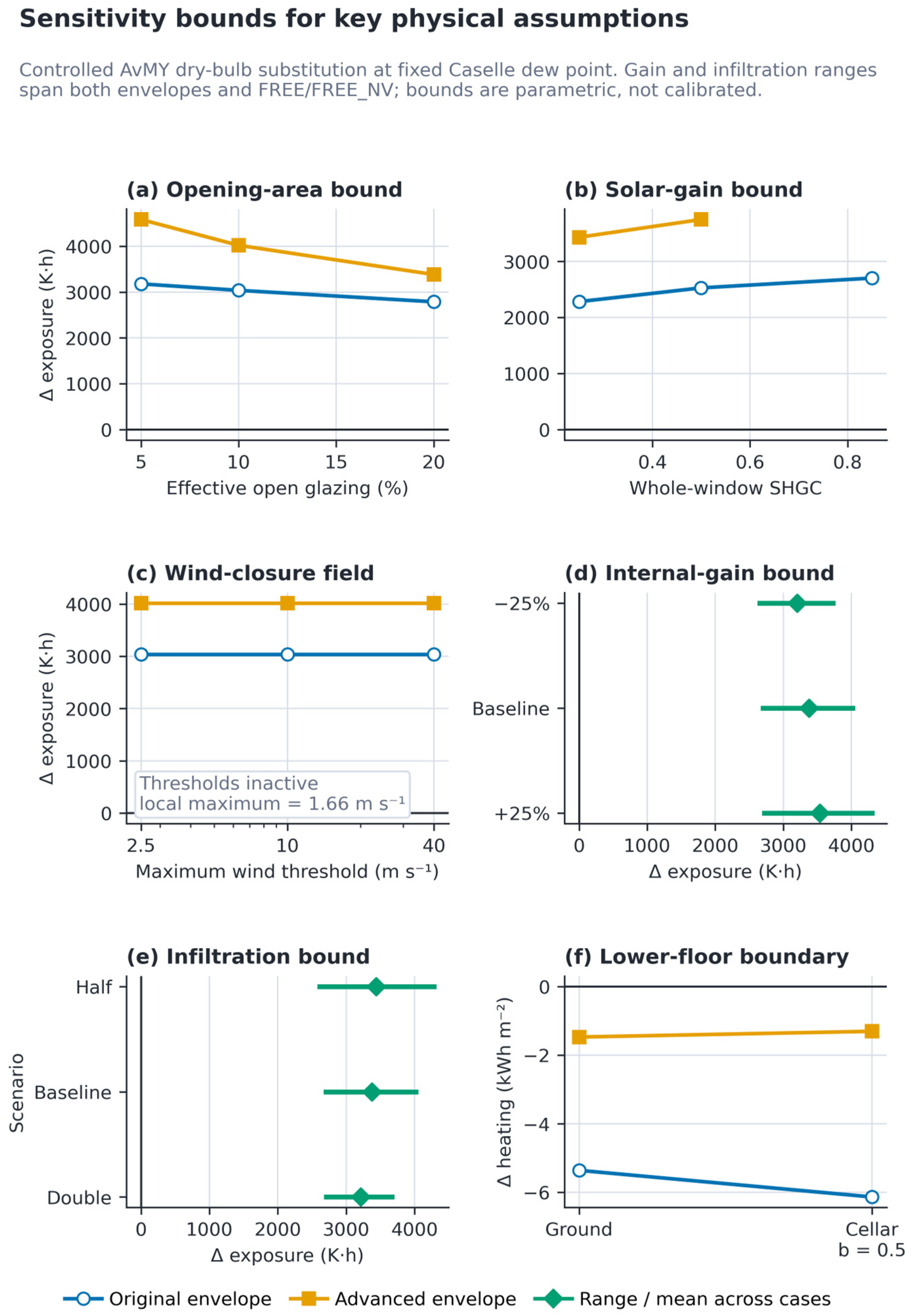
Figure A2.
Robustness of the eight principal ten-year Consolata-minus-Caselle relationships. Filled circles show full-data Pearson r, horizontal lines show the complete leave-one-year-out Pearson range, and open squares show Kendall’s τ_b. All coefficient signs remain stable after omitting any source year. The two UHI–degree-hour rows are mathematically coupled climate-consistency checks; the remaining rows relate climate indicators to dynamic building responses. Coefficients are descriptive for the fixed 2014–2023 source period.
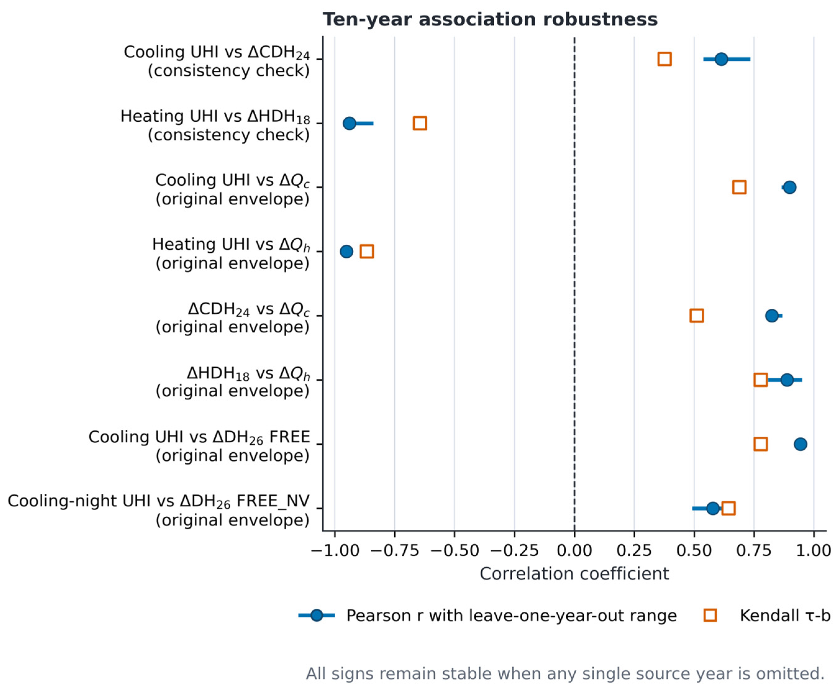
Figure A3.
Daily controlled Consolata-minus-Caselle AvMY relationships under TEMP_ONLY CUWF for the original and advanced envelopes: (a) SYS_ON useful sensible cooling; (b) SYS_ON useful sensible heating; (c) sealed FREE degree-hours above 26 °C; and (d) FREE_NV response-day degree-hours above 26 °C. Panels (a–c) use complete calendar days; panel (d) uses complete 19:00–19:00 response days. Lines are descriptive least-squares fits, and annotations report Pearson r, Kendall’s τ_b, and sample size. Aggregation reduces hourly density but not serial dependence and does not enlarge the ten-year AMY support.
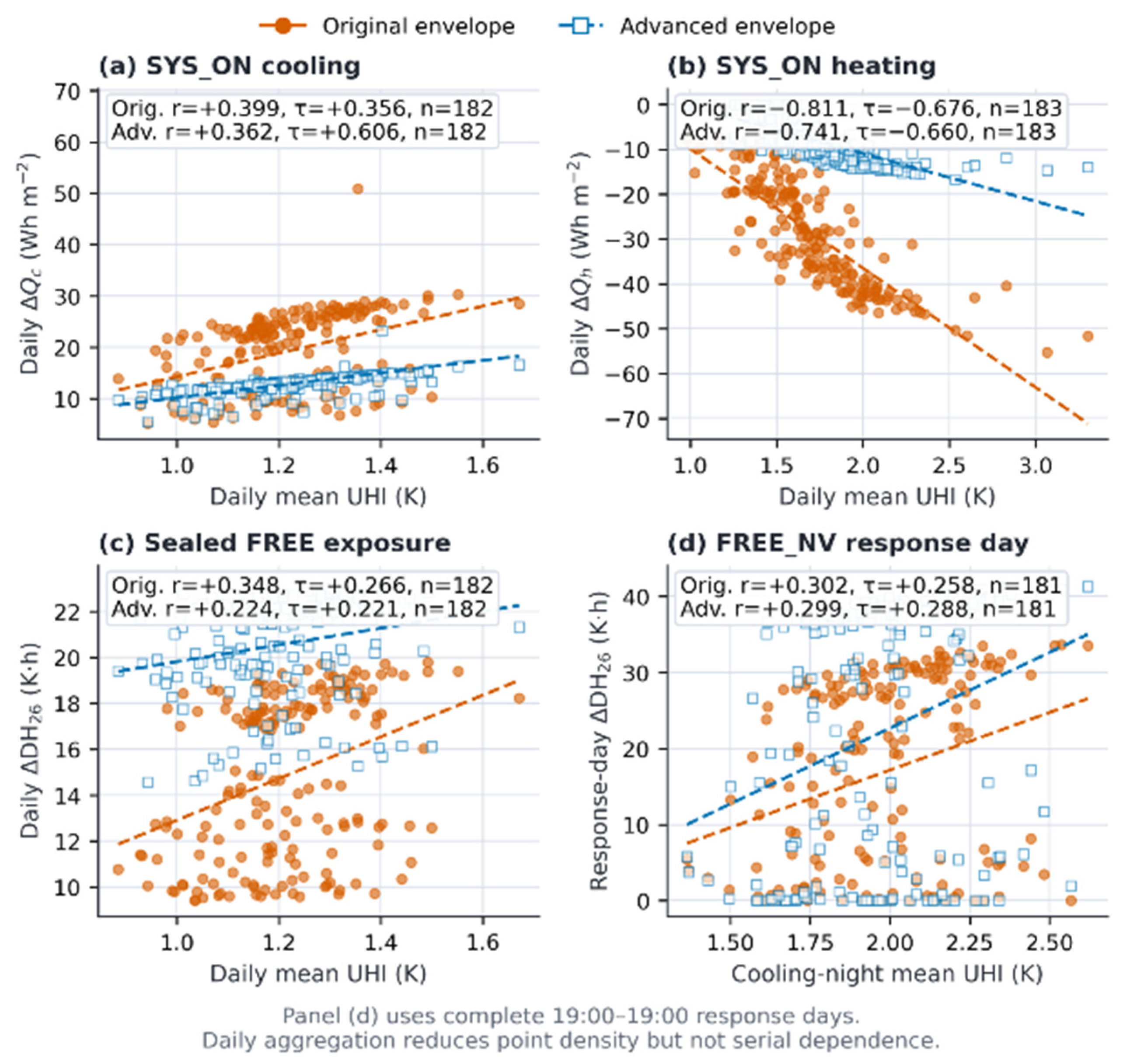
Figure A4.
Exploratory raw 0–24 h Pearson lag curves between Consolata–Caselle UHI and Consolata-minus-Caselle modelled response differences under TEMP_ONLY CUWF: (a) useful sensible cooling; (b) sealed FREE operative temperature; (c) FREE_NV operative temperature; and (d) the urban change in the FREE-to-FREE_NV operative-temperature benefit. Positive lag means UHI leads response. Original and advanced envelopes are shown separately. Raw peaks include shared seasonal, diurnal, and serial structure and must not be interpreted as causal delays; Figure 9 reports the month-by-hour-adjusted curves.
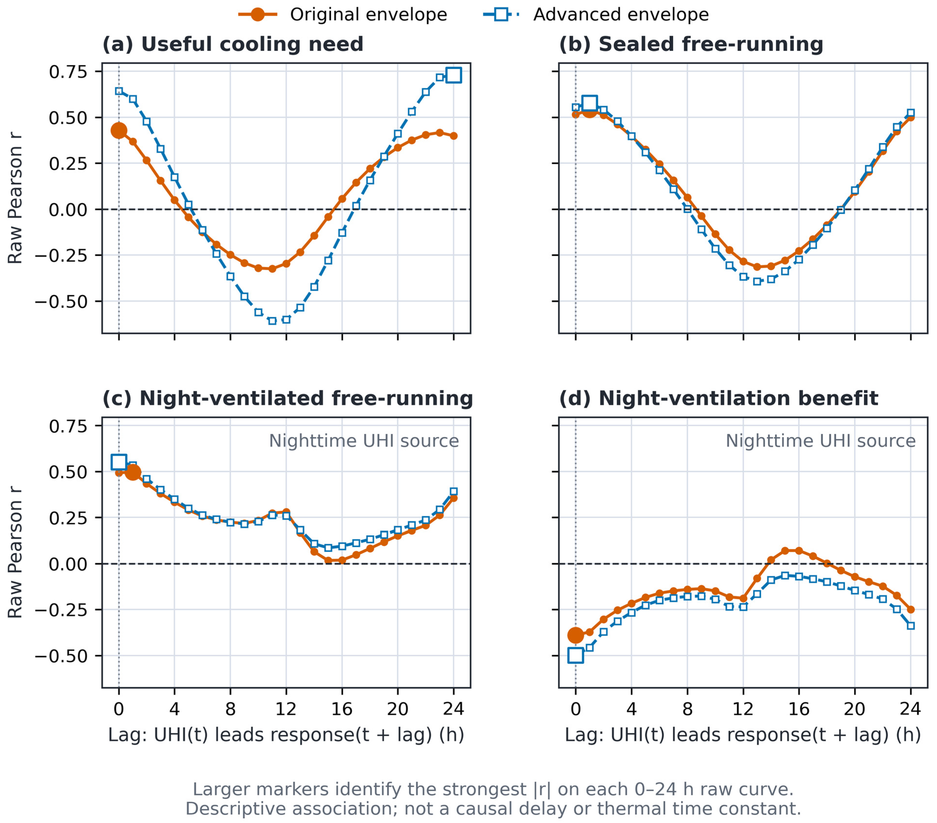
Table A2.
Incremental effect of substituting urban relative humidity, in addition to urban dry-bulb temperature, in the controlled AvMY simulations.
Table A3.
Descriptive correlations between declared UHI time intervals and matched-year building-response differences.
Table A4.
Night-ventilation activity and airflow diagnostics for the primary controlled AvMY cases.
Table A5.
Fixed geometry, internal-gain, infiltration, conditioning, and night-ventilation inputs for the DOE-derived/TABULA-envelope archetype.
Table A6.
Land-cover context around the seven meteorological stations at 100 and 500 m radii.
Table A7.
Station role, exposure, land-cover context, and quality-assurance qualification.
Table A8.
Weather-field provenance and forcing-manifest metadata. (a) Weather-family field provenance and interpretation boundary. (b) Machine-readable forcing and validation records.
Table A9.
Provenance and interpretation boundaries of the DOE–TABULA residential archetype.
Table A10.
Annual correlation coefficients and complete leave-one-year-out robustness checks. (a) Full ten-year coefficients. (b) Ranges across the ten nine-year leave-one-year-out subsets.
Table A11.
Daily aggregation and non-overlapping weekly sensitivity of the retained AvMY climate-to-building relationships. (a) Daily aggregation. (b) Non-overlapping weekly sensitivity.
Table A12.
Compact evidence-based uncertainty matrix.
References
- Oke, T.R. The energetic basis of the urban heat island. Q. J. R. Meteorol. Soc. 1982, 108, 1–24. [Google Scholar] [CrossRef] [Scilit]
- Stewart, I.D.; Oke, T.R. Local Climate Zones for urban temperature studies. Bull. Am. Meteorol. Soc. 2012, 93, 1879–1900. [Google Scholar] [CrossRef] [Scilit]
- World Meteorological Organization. Guidance on Measuring, Modelling and Monitoring the Urban Heat Island; WMO-No. 1292; WMO: Geneva, Switzerland, 2023. [Google Scholar]
- Huang, X.; Song, J. Urban moisture and dry islands: Spatiotemporal variation patterns and mechanisms of urban air humidity changes across the globe. Environ. Res. Lett. 2023, 18, 103003. [Google Scholar] [CrossRef] [Scilit]
- Santamouris, M.; Cartalis, C.; Synnefa, A.; Kolokotsa, D. On the impact of urban heat island and global warming on the power demand and electricity consumption of buildings—A review. Energy Build. 2015, 98, 119–124. [Google Scholar] [CrossRef] [Scilit]
- Li, X.; Zhou, Y.; Yu, S.; Jia, G.; Li, H.; Li, W. Urban heat island impacts on building energy consumption: A review of approaches and findings. Energy 2019, 174, 407–419. [Google Scholar] [CrossRef] [Scilit]
- Núñez Peiró, M.; Sánchez-Guevara Sánchez, C.; Neila González, F.J. Source area definition for local climate zones studies. A systematic review. Build. Environ. 2019, 148, 258–285. [Google Scholar] [CrossRef] [Scilit]
- Marinelli, L.; Cecilia, A.; Casasanta, G.; Conidi, A.; Petenko, I.; Argentini, S. Temperature Differences Between Rooftop and Urban Canyon Sensors: Diurnal Dynamics, Drivers, and Implications. Sensors 2025, 25, 4121. [Google Scholar] [CrossRef] [Scilit] [PubMed]
- Chan, A.L.S. Developing a modified typical meteorological year weather file for Hong Kong taking into account the urban heat island effect. Build. Environ. 2011, 46, 2434–2441. [Google Scholar] [CrossRef] [Scilit]
- Bueno, B.; Norford, L.; Hidalgo, J.; Pigeon, G. The urban weather generator. J. Build. Perform. Simul. 2013, 6, 269–281. [Google Scholar] [CrossRef] [Scilit]
- Tang, Y.; Sun, T.; Luo, Z.; Omidvar, H.; Theeuwes, N.; Xie, X.; Xiong, J.; Yao, R.; Grimmond, S. Urban meteorological forcing data for building energy simulations. Build. Environ. 2021, 204, 108088. [Google Scholar] [CrossRef] [Scilit]
- Wang, W.; Li, S.; Guo, S.; Ma, M.; Feng, S.; Bao, L. Benchmarking urban local weather with long-term monitoring compared with weather datasets from climate station and EnergyPlus weather (EPW) data. Energy Rep. 2021, 7, 6501–6514. [Google Scholar] [CrossRef] [Scilit]
- Chen, X.; Wang, T.; Wong, N.H.; Ang, Y.Q. Incorporating localized weather station data for microclimate-integrated urban building energy modeling: A campus-scale decarbonization study. Build. Environ. 2026, 290, 114150. [Google Scholar] [CrossRef] [Scilit]
- Su, M.A.; Ngarambe, J.; Santamouris, M.; Yun, G.Y. Empirical evidence on the impact of urban overheating on building cooling and heating energy consumption. iScience 2021, 24, 102495. [Google Scholar] [CrossRef] [Scilit] [PubMed]
- Salvati, A.; Coch Roura, H.; Cecere, C. Assessing the urban heat island and its energy impact on residential buildings in Mediterranean climate: Barcelona case study. Energy Build. 2017, 146, 38–54. [Google Scholar] [CrossRef] [Scilit]
- Paolini, R.; Zani, A.; MeshkinKiya, M.; Castaldo, V.L.; Pisello, A.L.; Antretter, F.; Poli, T.; Cotana, F. The hygrothermal performance of residential buildings at urban and rural sites: Sensible and latent energy loads and indoor environmental conditions. Energy Build. 2017, 152, 792–803. [Google Scholar] [CrossRef] [Scilit]
- Cui, Y.; Yan, D.; Hong, T.; Ma, J. Temporal and spatial characteristics of the urban heat island in Beijing and the impact on building design and energy performance. Energy 2017, 130, 286–297. [Google Scholar] [CrossRef] [Scilit]
- Yang, X.; Peng, L.L.H.; Jiang, Z.; Chen, Y.; Yao, L.; He, Y.; Xu, T. Impact of urban heat island on energy demand in buildings: Local climate zones and multi-site observations. Appl. Energy 2020, 260, 114279. [Google Scholar] [CrossRef] [Scilit]
- Hong, T.; Xu, Y.; Sun, K.; Zhang, W.; Luo, X.; Hooper, B. Urban microclimate and its impact on building performance: A case study of San Francisco. Urban Clim. 2021, 38, 100871. [Google Scholar] [CrossRef] [Scilit]
- Zinzi, M.; Carnielo, E.; Mattoni, B. On the relation between urban climate and energy performance of buildings. A three-years experience in Rome, Italy. Appl. Energy 2018, 221, 148–160. [Google Scholar] [CrossRef] [Scilit]
- Battista, G.; Evangelisti, L.; Guattari, C.; Roncone, M.; Balaras, C.A. Space-time estimation of the urban heat island in Rome (Italy): Overall assessment and effects on the energy performance of buildings. Build. Environ. 2023, 228, 109878. [Google Scholar] [CrossRef] [Scilit]
- Guattari, C.; Evangelisti, L.; Balaras, C.A. On the assessment of urban heat island phenomenon and its effects on building energy performance: A case study of Rome (Italy). Energy Build. 2018, 158, 605–615. [Google Scholar] [CrossRef] [Scilit]
- Ma, Y.X.; Yu, A.C. Impact of urban heat island on high-rise residential building cooling energy demand in Hong Kong. Energy Build. 2024, 311, 114127. [Google Scholar] [CrossRef] [Scilit]
- Sharston, R.; Singh, M. The role of passive, active, and operational parameters in the relationship between urban heat island effect and building energy consumption. Energy Build. 2024, 323, 114720. [Google Scholar] [CrossRef] [Scilit]
- Zou, Y.; Wu, Z.; Li, B.; Jia, Y. Cooling energy challenges in residential buildings during heat waves: Urban heat island impacts in a hot-humid city. Buildings 2024, 14, 4030. [Google Scholar] [CrossRef] [Scilit]
- JahaniRahaei, A.; Milelli, M.; Chiesa, G. Urban weather dataset for building energy simulations: Data collection and EPW file generation for Torino, Italy (2014–2023). Data Brief 2025, 61, 111708. [Google Scholar] [CrossRef] [Scilit] [PubMed]
- Milelli, M.; Bassani, F.; Garbero, V.; Poggi, D.; von Hardenberg, J.; Ridolfi, L. Characterization of the Urban Heat and Dry Island effects in the Turin metropolitan area. Urban Clim. 2023, 47, 101397. [Google Scholar] [CrossRef] [Scilit]
- Bassani, F.; Garbero, V.; Poggi, D.; Ridolfi, L.; von Hardenberg, J.; Milelli, M. An innovative approach to select urban-rural sites for Urban Heat Island analysis: The case of Turin (Italy). Urban Clim. 2022, 42, 101099. [Google Scholar] [CrossRef] [Scilit]
- Li, D.; Wang, L.; Liao, W.; Sun, T.; Katul, G.; Bou-Zeid, E.; Maronga, B. Persistent urban heat. Sci. Adv. 2024, 10, eadj7398. [Google Scholar] [CrossRef] [Scilit] [PubMed]
- Peerlings, E.E.M.; Steeneveld, G.J. Unravelling indoor temperature response to summer heat through long-term crowdsourced observations in Dutch residences. Q. J. R. Meteorol. Soc. 2026, 152, e70053. [Google Scholar] [CrossRef] [Scilit]
- Kolokotroni, M.; Giannitsaris, I.; Watkins, R. The effect of the London urban heat island on building summer cooling demand and night ventilation strategies. Sol. Energy 2006, 80, 383–392. [Google Scholar] [CrossRef] [Scilit]
- Artmann, N.; Manz, H.; Heiselberg, P. Climatic potential for passive cooling of buildings by night-time ventilation in Europe. Appl. Energy 2007, 84, 187–201. [Google Scholar] [CrossRef] [Scilit]
- Chiesa, G.; Li, Y. Including Urban Heat Island in Bioclimatic Early-Design Phases: A Simplified Methodology and Sample Applications. Sustainability 2021, 13, 5918. [Google Scholar] [CrossRef] [Scilit]
- Ramponi, R.; Gaetani, I.; Angelotti, A. Influence of the urban environment on the effectiveness of natural night-ventilation of an office building. Energy Build. 2014, 78, 25–34. [Google Scholar] [CrossRef] [Scilit]
- Xie, X.; Sahin, O.; Luo, Z.; Yao, R. Impact of neighbourhood-scale climate characteristics on building heating demand and night ventilation cooling potential. Renew. Energy 2020, 150, 943–956. [Google Scholar] [CrossRef] [Scilit]
- Zinzi, M.; Agnoli, S.; Romano, S.; Siani, A.M.; Falasca, S. On the impact urban modified albedo: Comparing the thermal conditions and the night ventilation potential in urban and rural dwellings in Rome, Italy. Int. J. Vent. 2026, 25, 44–59. [Google Scholar] [CrossRef] [Scilit]
- Chiesa, G.; von Hardenberg, J. Including climate change time-dimensions in bioclimatic design. TECHNE J. Technol. Archit. Environ. 2020, 20, 204–212. [Google Scholar] [CrossRef] [Scilit]
- Wilcox, S.; Marion, W. Users Manual for TMY3 Data Sets (Revised); NREL/TP-581-43156; National Renewable Energy Laboratory: Golden, CO, USA, 2008. [Google Scholar] [CrossRef] [Scilit]
- Libralato, M.; Murano, G.; De Angelis, A.; Saro, O.; Corrado, V. Influence of the Meteorological Record Length on the Generation of Representative Weather Files. Energies 2020, 13, 2103. [Google Scholar] [CrossRef] [Scilit]
- Siu, C.Y.; Liao, Z. Is building energy simulation based on TMY representative: A comparative simulation study on DOE reference buildings in Toronto with typical year and historical year type weather files. Energy Build. 2020, 211, 109760. [Google Scholar] [CrossRef] [Scilit]
- Evola, G.; Costanzo, V.; Infantone, M.; Marletta, L. Typical-year and multi-year building energy simulation approaches: A critical comparison. Energy 2021, 219, 119591. [Google Scholar] [CrossRef] [Scilit]
- Kittner, J.; Fenner, D.; Demuzere, M.; Bechtel, B. Finding the sea level—Investigation of rural references for estimation of the urban heat island. PLoS Clim. 2026, 5, e0000955. [Google Scholar] [CrossRef] [Scilit]
- ARPA Piemonte. Meteoidro API: Stazione_Meteorologica Catalogue and OpenAPI Schema. Available online: https://utility.arpa.piemonte.it/meteoidro/stazione_meteorologica/ (accessed on 24 July 2026).
- Regione Piemonte. Land Cover Piemonte: Classificazione di Uso e Copertura del Suolo, 2021 ed.; Regione Piemonte: Torino, Italy; Available online: https://www.geoportale.piemonte.it/geonetwork/serv/api/records/r_piemon%3A35df8a16-5d89-461f-a0f2-abc2180713d2 (accessed on 24 July 2026).
- Zhang, S.; Liu, N.; Wu, X.; Han, Y.; Li, W.; Guo, F.; Song, X.; Yuan, C. An empirical study on the compound effects of extreme weather and UHI on building energy consumption under urban local climate. Build. Environ. 2026, 287, 113824. [Google Scholar] [CrossRef] [Scilit]
- Chiesa, G.; Kolokotroni, M.; Heiselberg, P. (Eds.) Innovations in Ventilative Cooling; Springer: Cham, Switzerland, 2021. [Google Scholar] [CrossRef] [Scilit]
- Deru, M.; Field, K.; Studer, D.; Benne, K.; Griffith, B.; Torcellini, P.; Liu, B.; Halverson, M.; Winiarski, D.; Rosenberg, M.; et al. U.S. Department of Energy Commercial Reference Building Models of the National Building Stock; NREL/TP-5500-46861; National Renewable Energy Laboratory: Golden, CO, USA, 2011. [Google Scholar] [CrossRef] [Scilit] [PubMed]
- U.S. Department of Energy. EnergyPlus™ (SWR-17-23), Version 26.1.0; National Laboratory of the Rockies: Golden, Colorado, 2017. [CrossRef]
- Shen, P.; Wang, H. Archetype building energy modeling approaches and applications: A review. Renew. Sustain. Energy Rev. 2024, 199, 114478. [Google Scholar] [CrossRef] [Scilit]
- Ballarini, I.; Corgnati, S.P.; Corrado, V. Use of reference buildings to assess the energy saving potentials of the residential building stock: The experience of TABULA project. Energy Policy 2014, 68, 273–284. [Google Scholar] [CrossRef] [Scilit]
- Corrado, V.; Ballarini, I.; Corgnati, S.P. Building Typology Brochure—Italy. Fascicolo Sulla Tipologia Edilizia Italiana. Nuova Edizione; Politecnico di Torino: Turin, Italy, 2014; pp. 115–116. [Google Scholar]
- Stermieri, L.; Delmastro, C.; Becchio, C.; Corgnati, S.P. Linking dynamic building simulation with long-term energy system planning to improve buildings urban energy planning strategies. Smart Cities 2020, 3, 1242–1265. [Google Scholar] [CrossRef] [Scilit]
- Ballarini, I.; Costantino, A.; Fabrizio, E.; Corrado, V. A methodology to investigate the deviations between simple and detailed dynamic methods for the building energy performance assessment. Energies 2020, 13, 6217. [Google Scholar] [CrossRef] [Scilit]
- Prataviera, E.; Vivian, J.; Lombardo, G.; Zarrella, A. Evaluation of the impact of input uncertainty on urban building energy simulations using uncertainty and sensitivity analysis. Appl. Energy 2022, 311, 118691. [Google Scholar] [CrossRef] [Scilit]
- Mugnini, A.; Ramallo-González, A.P.; Molina García, Á.; Arteconi, A. An integrated approach to assess thermal mass and passive cooling: Mapping cooling need and overheating risk under climate change scenarios. Build. Environ. 2026, 287, 113843. [Google Scholar] [CrossRef] [Scilit]
- Lomas, K.J.; Li, M.; Drury, P. How do energy efficiency measures affect the risk of summertime overheating and cold discomfort? Evidence from English homes. Energy Policy 2024, 188, 114108. [Google Scholar] [CrossRef] [Scilit]
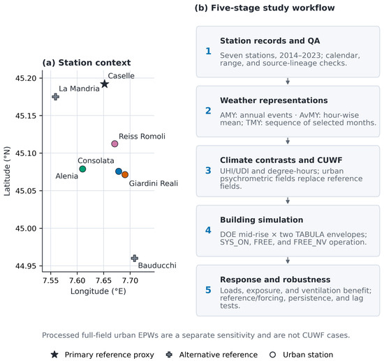
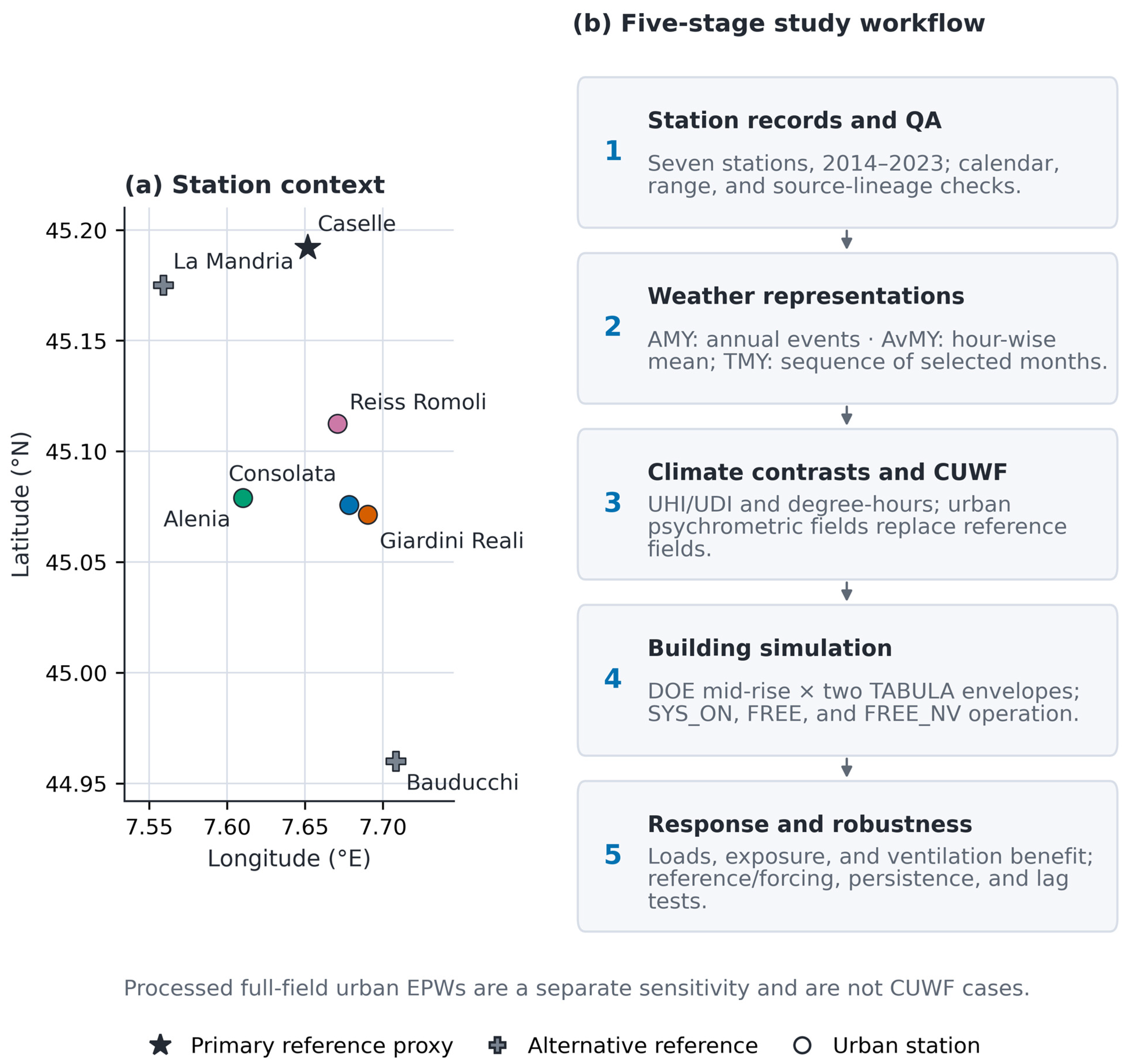
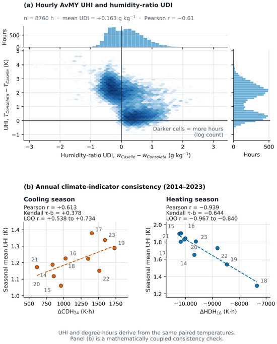
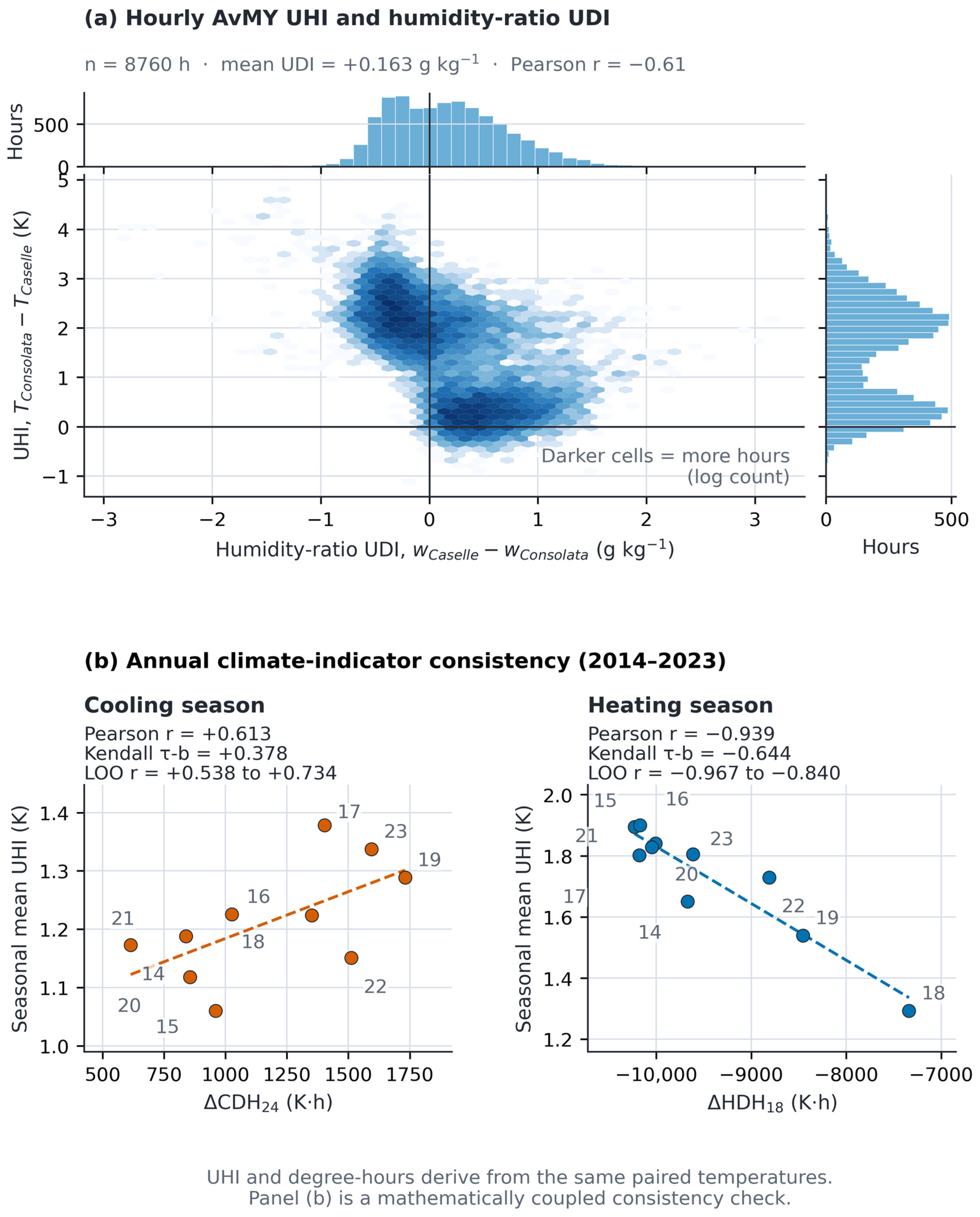
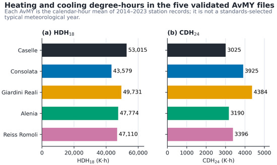
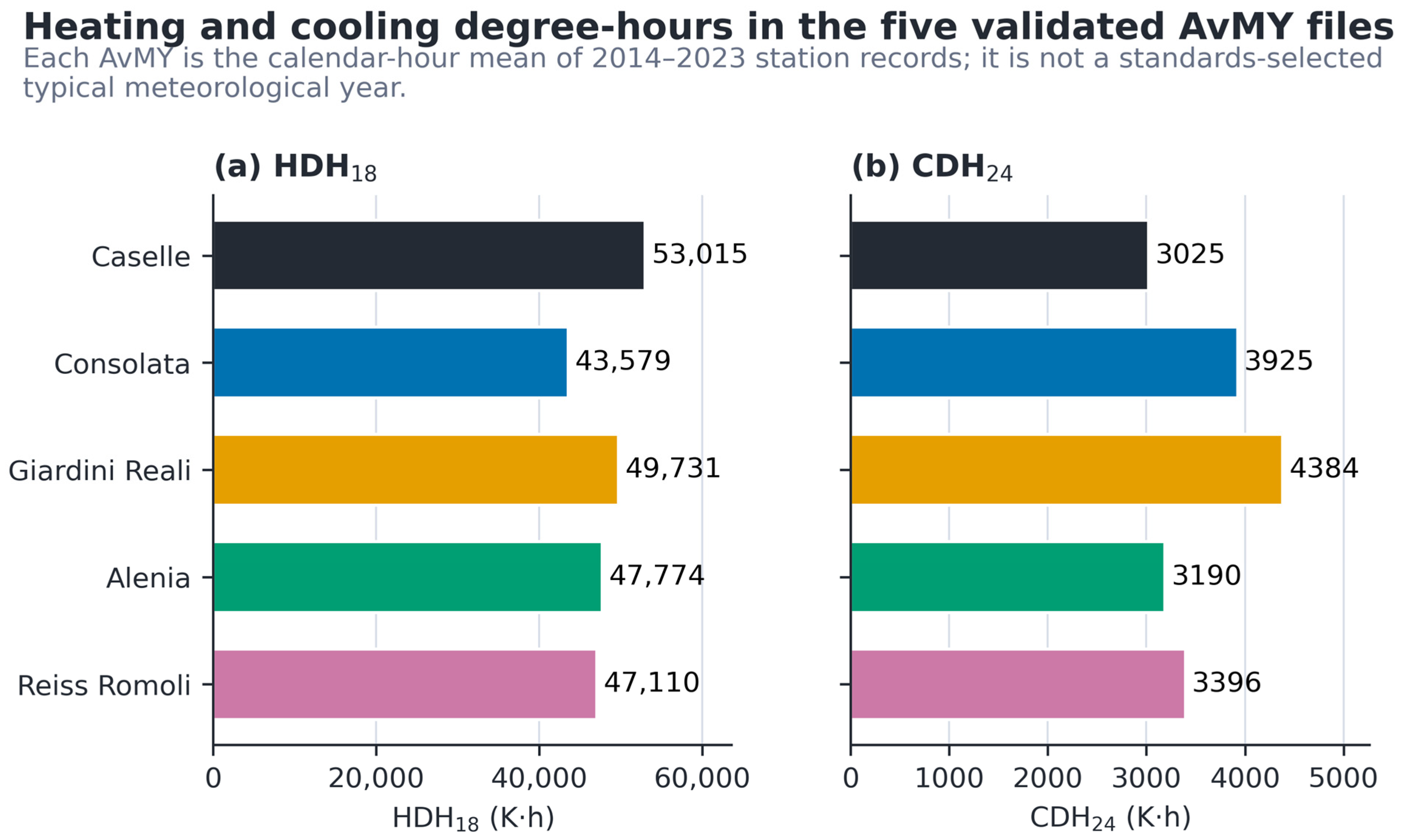
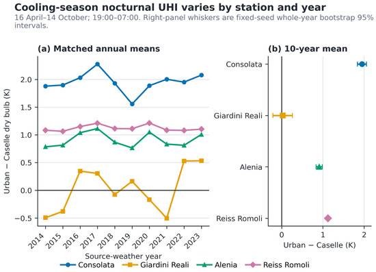
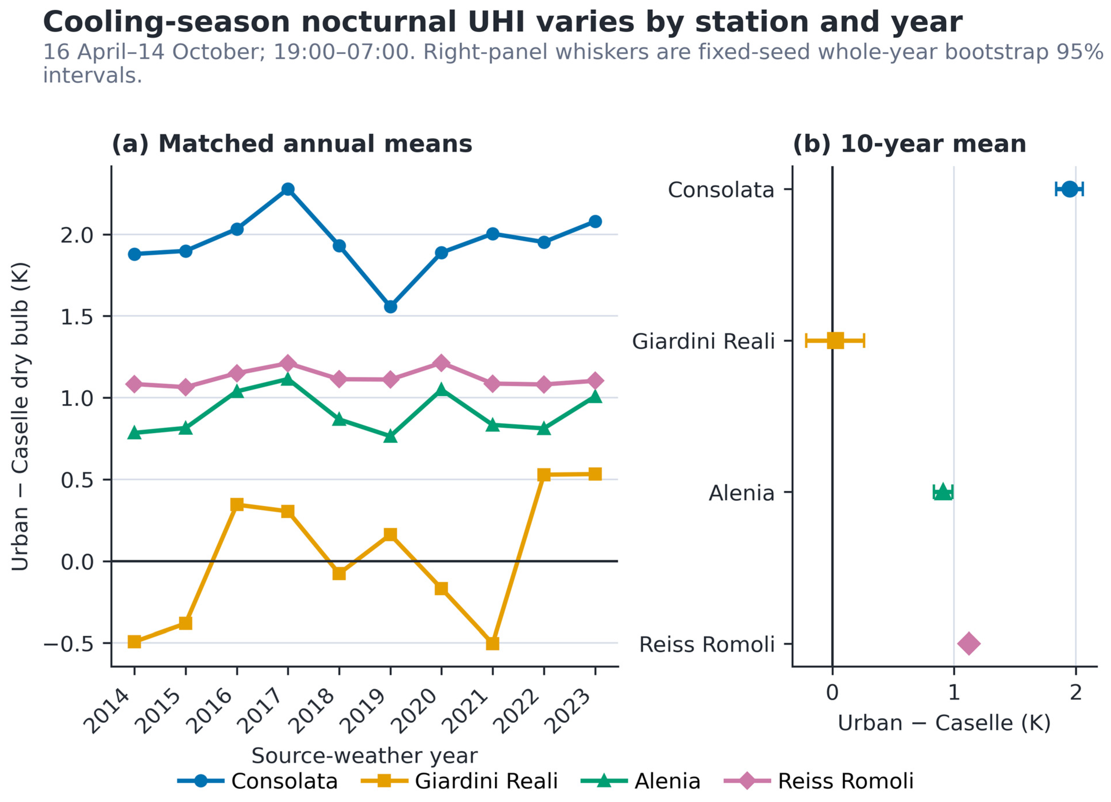
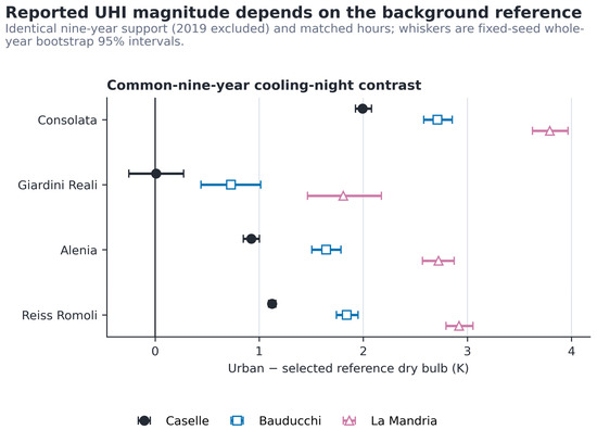
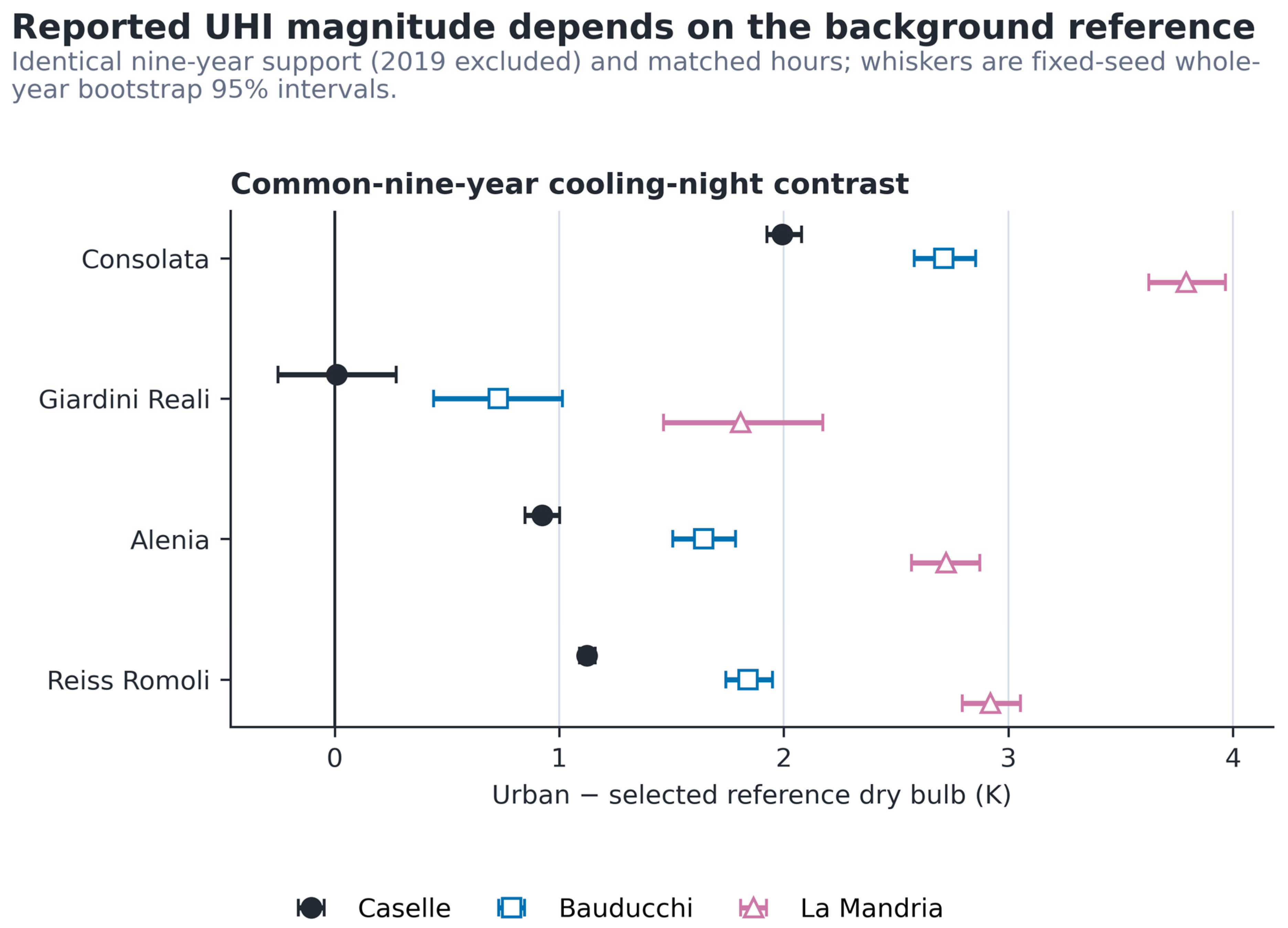
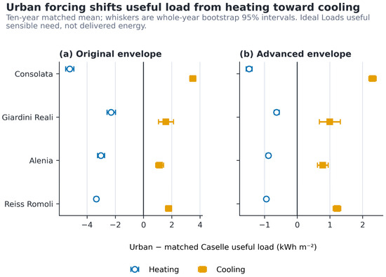
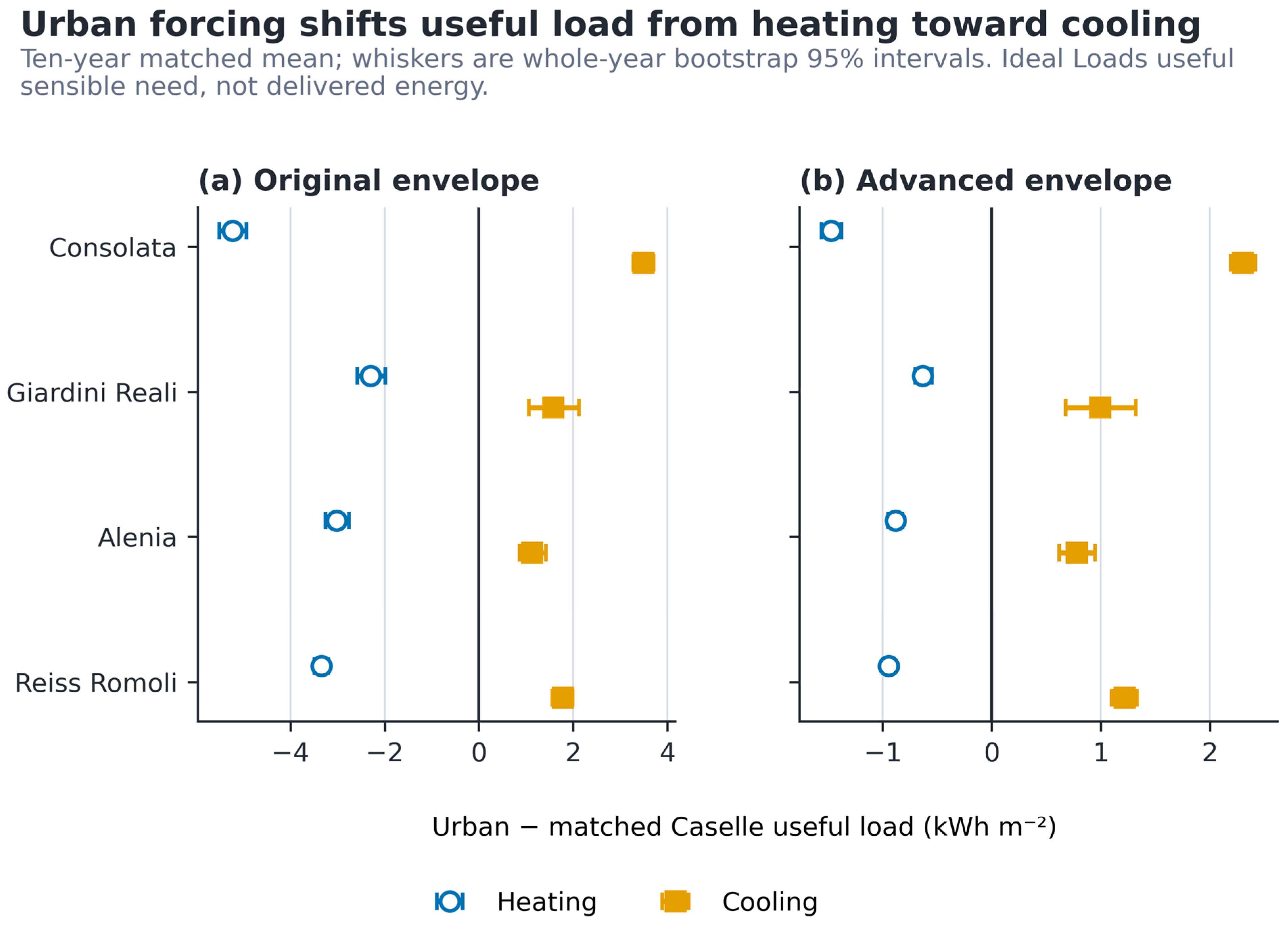
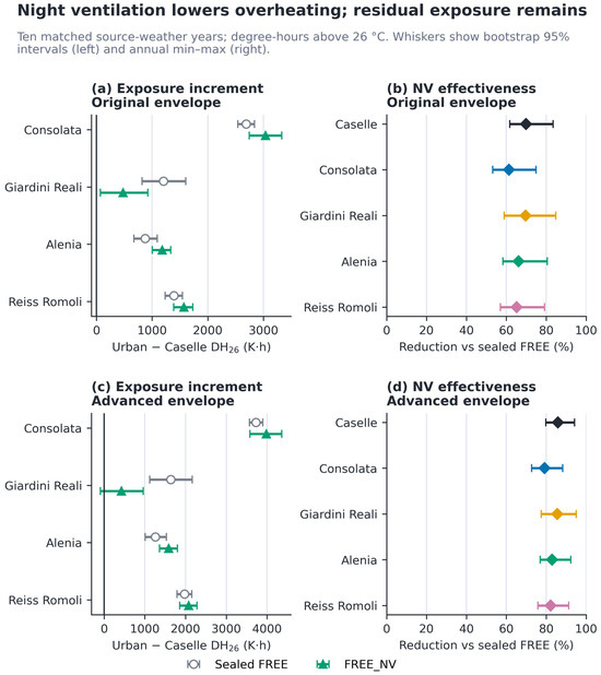
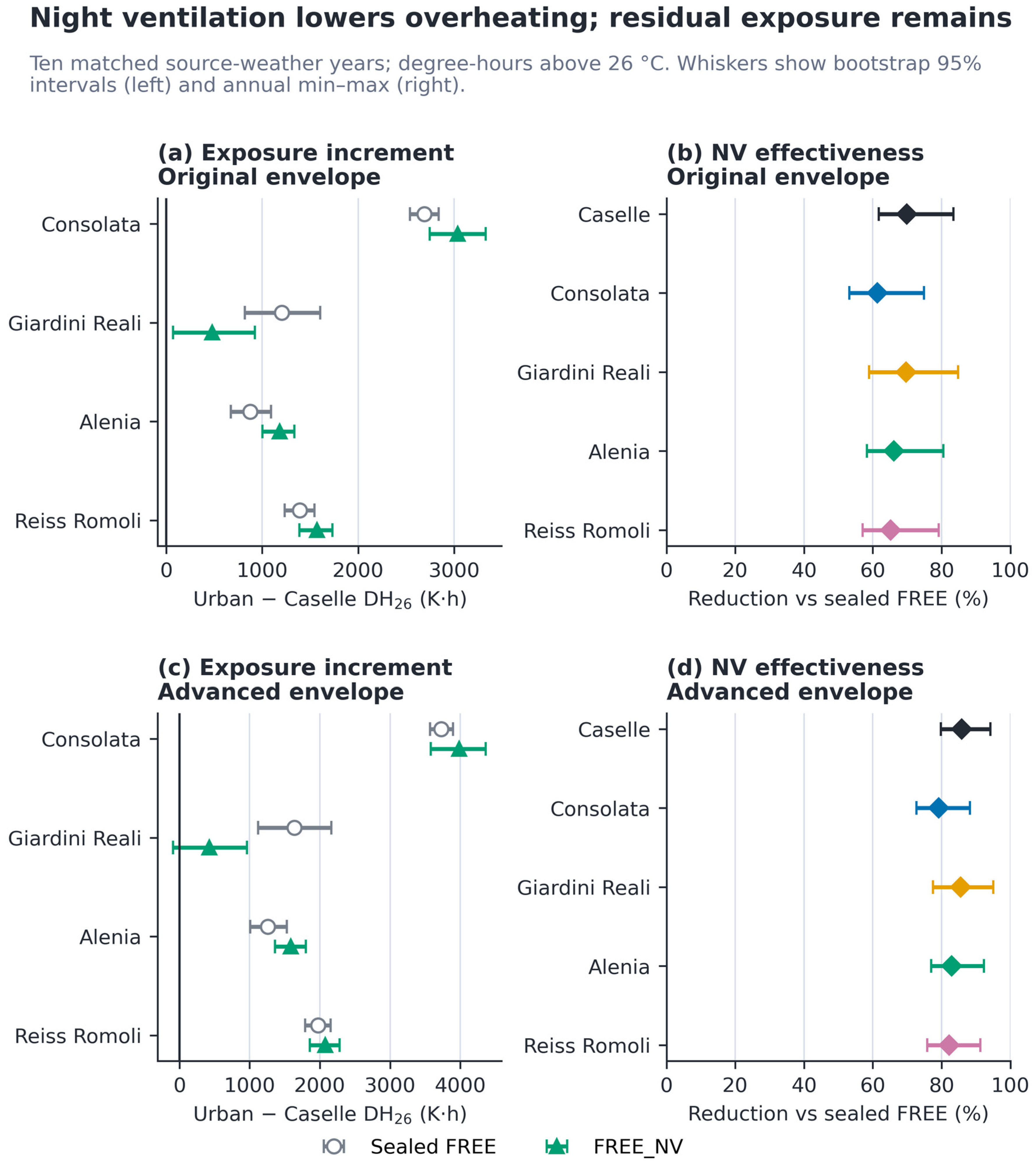
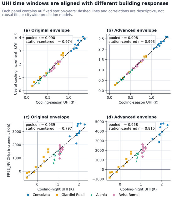
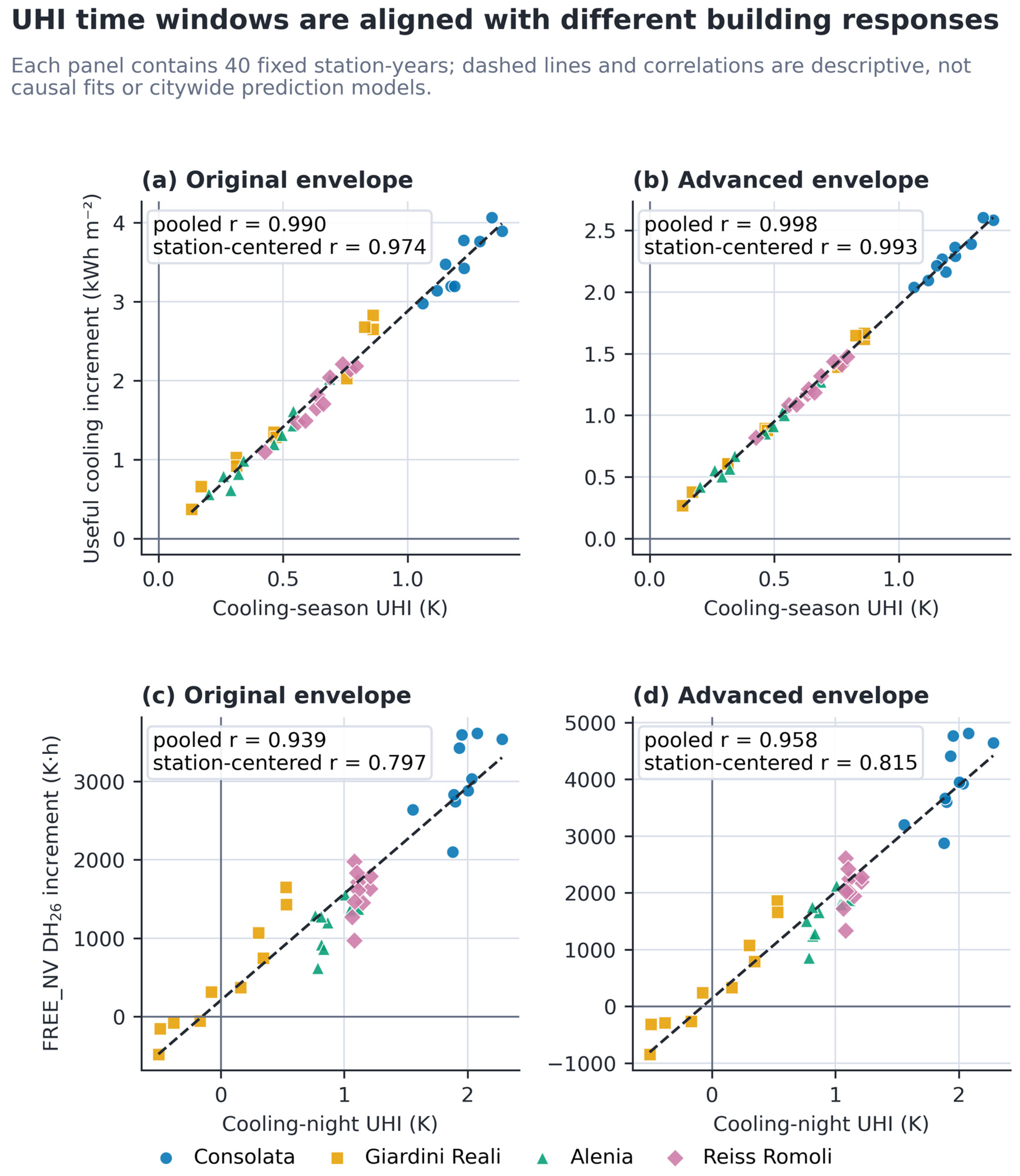
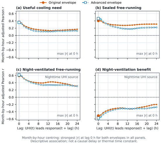
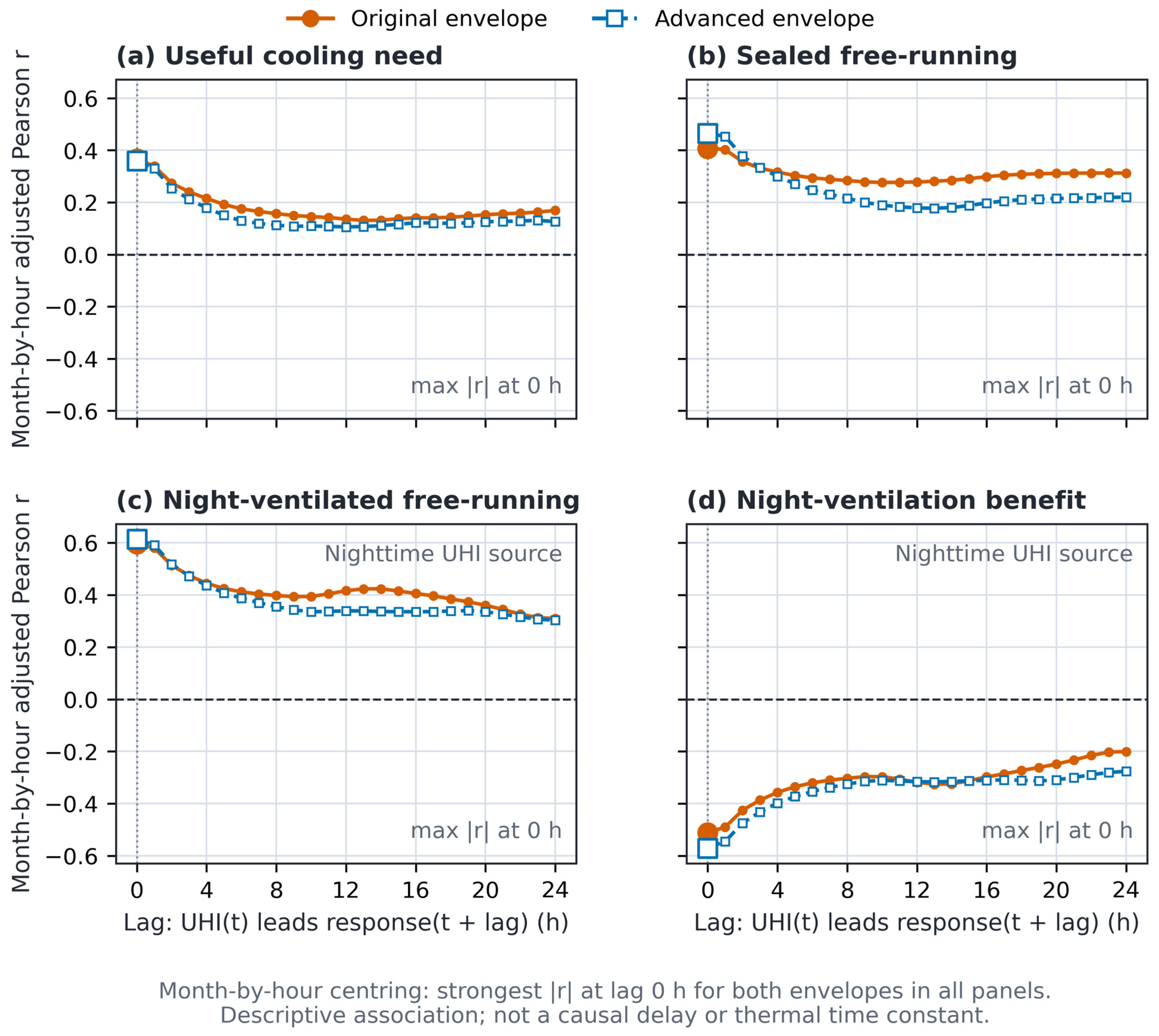
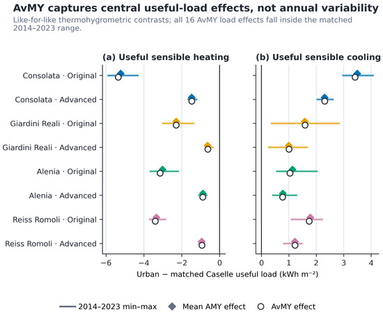
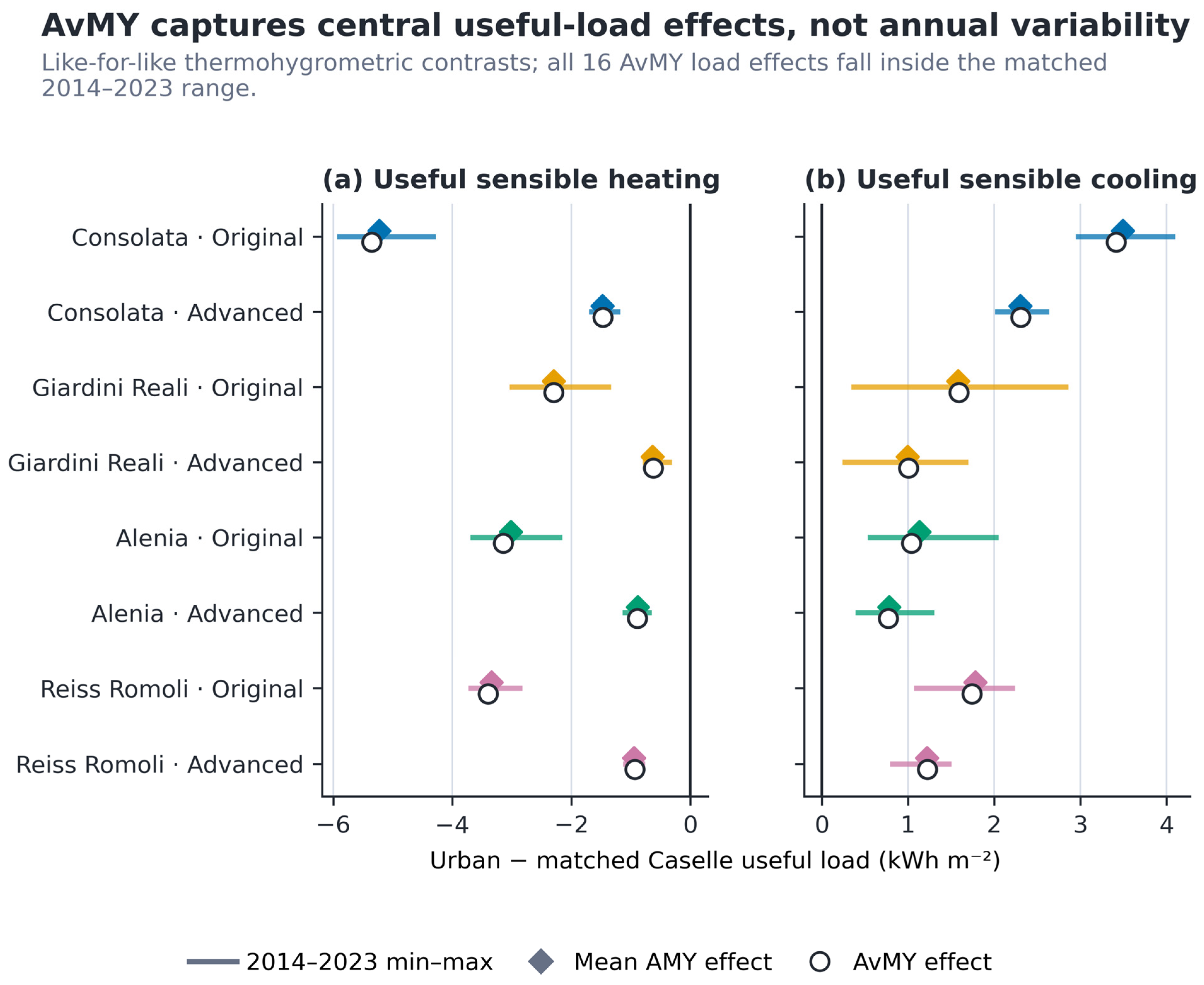
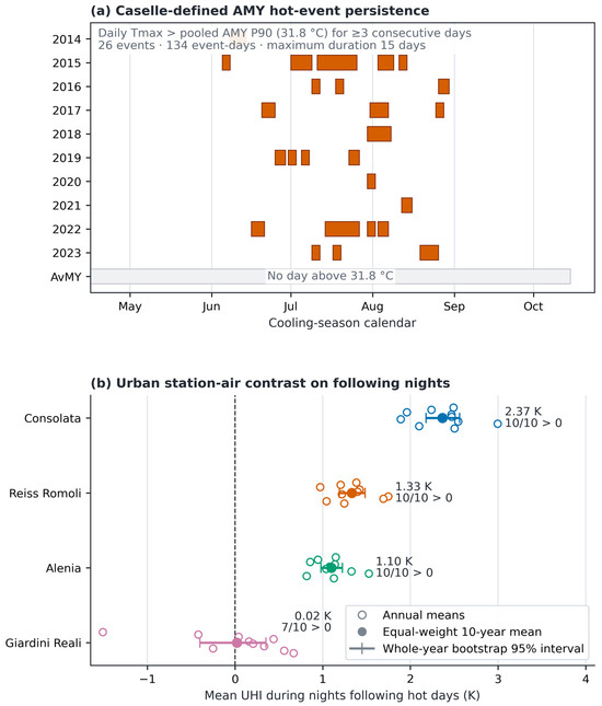
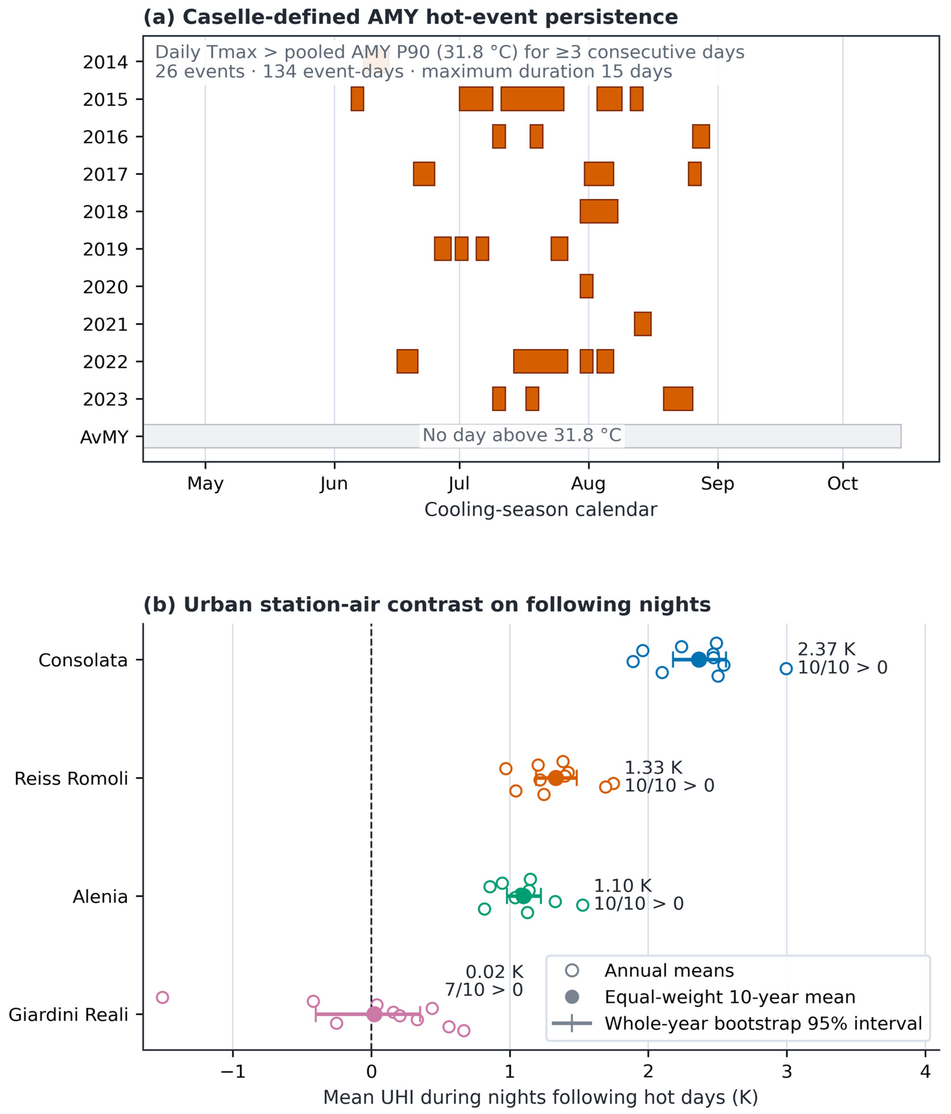
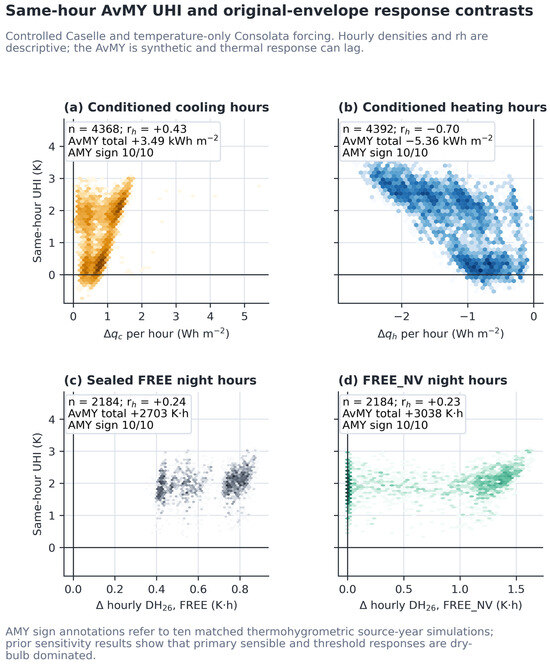
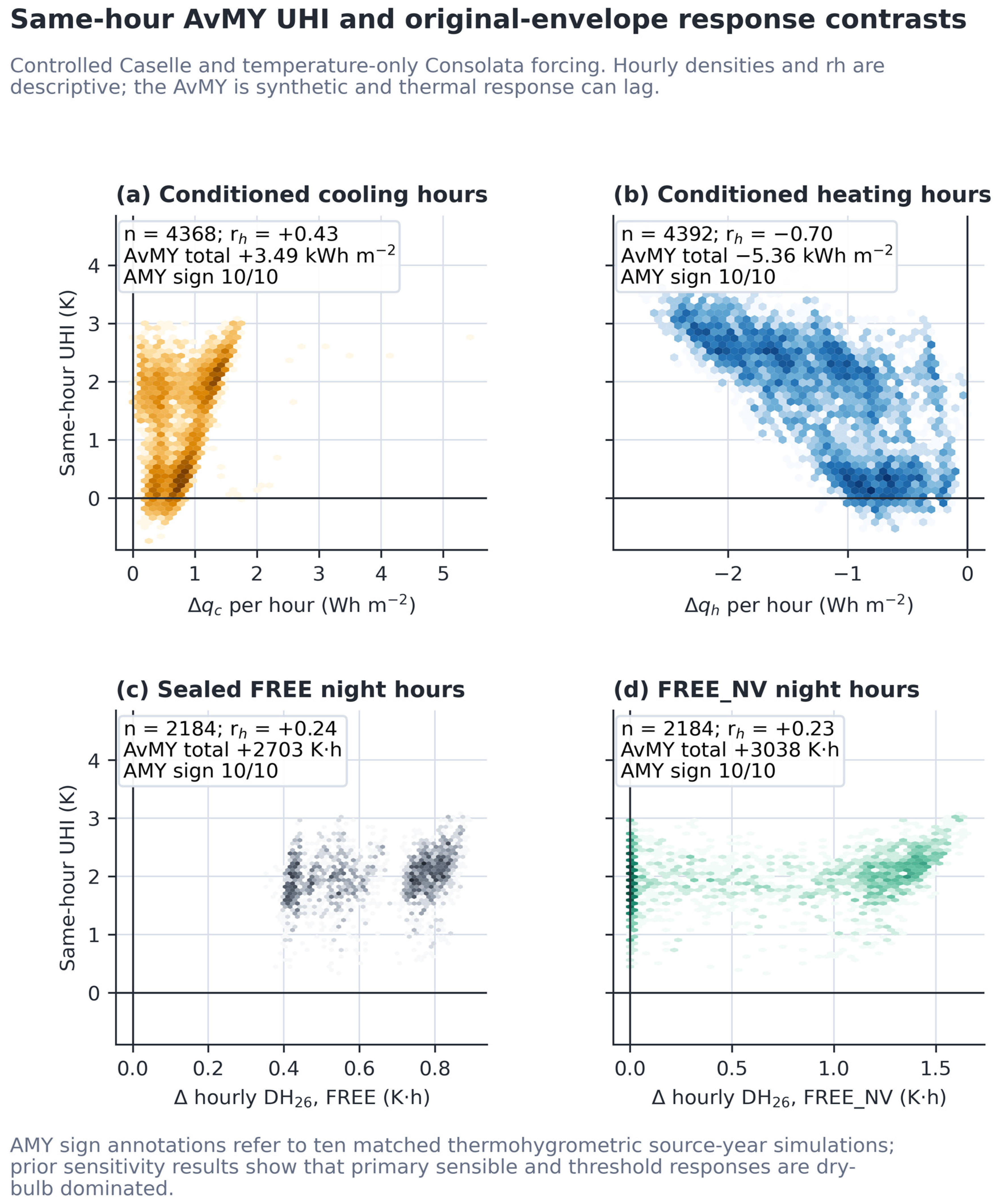

Disclaimer/Publisher’s Note: The statements, opinions and data contained in all publications are solely those of the individual author(s) and contributor(s) and not of MDPI and/or the editor(s). MDPI and/or the editor(s) disclaim responsibility for any injury to people or property resulting from any ideas, methods, instructions or products referred to in the content. |
© 2026 by the authors. Licensee MDPI, Basel, Switzerland. This article is an open access article distributed under the terms and conditions of the Creative Commons Attribution (CC BY) license.