


Abstract
Evaluating spatiotemporal dynamics is essential to measure and monitor environmental sustainability in coastal zones under rapid urban expansion. Future scenarios of the earth’s surface can be estimated from identified changes in remote sensing. The objectives of this study were to evaluate changes in the land surface temperature (LST), estimated with Landsat 8 images of the Brazilian coastal municipality of Arraial do Cabo on two summer dates—2014 and 2017—and to project a scenario for 2030. Data processing was performed in the open GIS QGIS version 3.2.0, while the comparison and the future projection were performed with Land Change Modeler tools in the commercial GIS IDRISI Selva version 17.0. Spatial analysis revealed a unilateral expansion of the ‘heat’ class and a simultaneous contraction of the ‘coolness’ class, revealing a severe loss of local microclimatic sustainability. The prediction of the Markov matrix for 2030 indicated a 98.9% probability of transition from the medium to the heat class and a 96.9% probability of transition from the coolness to the heat class, highlighting the critical vulnerability of coastal environmental indicators. It also showed more urban areas replacing green areas, salt ponds and exposed soil. These trends warn of negative environmental impacts on the native ecosystem, the local state park, and Araruama Lagoon, which may influence LST. Effective environmental conservation policies are essential to guarantee ecological sustainability, mitigating the loss of vegetated areas and regulating local surface temperatures for long-term climate resilience. Projections related to different environmental issues should include other factors to be applied to environmental planning. This study is presented as a preliminary exploratory analysis. The 2030 projection represents a conditional scenario demonstrating the potential impacts if the extreme short-term transitions observed between 2014 and 2017 were to continue. These baseline findings highlight the sensitivity of the coastal environment and underscore the need for future robust time-series modeling.
1. Introduction
Studies and techniques related to urban climates have advanced significantly over the last decades, considering factors like local winds, radiation, energy balance, water balance, humidity and condensation [1,2,3]. The urban surface heat accumulation is the main phenomenon in this scale of analysis, one of the key topics of Urban Climatology studies [4]. According to Ren et al. [5], the introduction of studies of the urban climate map was proposed to support the implementation of mitigation guidelines and measures focused on local planning.
Initial investigations into the urban climate of Rio de Janeiro were conducted by Gallego [6] and Brandão [7,8], paving the way for subsequent applied academic research [9,10,11]. Marques Filho et al. [12] analyzed the thermodynamics and its time evolution in the Metropolitan Area of Rio de Janeiro, while Karam et al. [13] simulated the diurnal surface heat accumulation in this region using an urban meteorological model and observed data. In this context, integrating urban climatology with sustainable development goals is crucial for coastal cities. Monitoring land surface temperature (LST) and land cover (LC) dynamics represents a vital sustainability tool for defining local ecological limits and guiding territorial policies that mitigate microclimatic degradation.
Cui and Shi [14] presented ecological and climatic factors correlated to urbanization using remote sensing data for land use, LC, and LST; meteorological station data; and social statistical data in Shanghai, China. Pacifici et al. [15] indicated higher microclimatic influence by high-rise building exposure in the Metropolitan Area of Sao Paulo, while Ferreira and Duarte [16] explored the relationship between daytime and nighttime LST and the urban morphology, showing a strong negative correlation between LST and vegetation indexes, as well as a positive correlation of nighttime LST and building surface fraction and impervious surface, consequences of urbanization.
Urban climate modeling gathers climate information, land use data and land surface data, creating more comprehensive analyses and climate assessments, which can be considered in urban planning [5]. In Brazil, Katzschner et al. [17] studied LST in the urban planning of Salvador, while Tarifa and Armani [18] investigated the city of São Paulo. To analyze the spatial distribution and patterns of LST, Sousa and Ferreira [19] compared thermal anomaly images for the Brazilian municipality of Goiania. Moreover, studies of surface heat evolved with better spatial resolution of thermal remote sensing and automatic correction of the images.
Land cover changes were reported in the Lake Region of the state of Rio de Janeiro, where the municipality of Arraial do Cabo is located [20,21]. Arraial do Cabo presented a population growth from 27,715 inhabitants in 2010 to 30,593 estimated for 2020 [22], as well as more plots of land mainly between the Atlantic Ocean and Araruama Lagoon [23,24]. However, there are no land use and land cover (LULC) or land cover (LC) scenarios nor other parameters estimated for the region.
A possible increase of the global mean temperature may affect cities that were not planned and that are in coastal areas. The years 2016, 2015 and 2017, in descending order, were considered the hottest years recorded since the Industrial Revolution until 2018 [25]. The Paris Agreement was signed in 2015 and came into force in 2016, aiming at promoting global strategies to respond to climate change until 2030 [26]. New research has since been developed with multitemporal analysis and mathematical projection.
In the projection proposed herein, future trends are generated by extrapolating the physical changes observed between two discrete temporal periods to generate a third instant, while the prediction requires a set of alternative scenarios with conditioning variables [27,28]. The scenarios from remote sensing data in geoprocessing can address different themes and have many applications. LULC or LC scenarios are more common than LST projections.
The Land Change Modeler (LCM) tool in the IDRISI GIS has been recommended for complex land cover changes analysis since it enables a combination of neural networks called Multi-Layer Perceptron and the Markov chain. Raster images from the first and second moments are necessary as inputs, and they can be obtained from other sources or generated by classifying images. In the LCM, it is possible to define weights to layers and then to projections and constraint areas. When the scenario is generated with only classified images, with no guiding factors, it is called a quantitative trend scenario.
The transition probabilities resulting from changes between scenes can be used to predict future scenarios [28,29,30,31,32,33,34,35,36]. Beser de Deus [28] assessed the green cover changes of the Acre River Basin, which spans over Brazil, Bolivia and Peru. The author considered conflicts and generated a LULC class prognostic with qualitative and quantitative data using traditional knowledge to elaborate scenarios of historical thematic cartography from 1904 up until the 1970s. Then, classified scenes from 1970 and 2010 were imported into IDRISI Selva version 17.0 to assess changes and generate scenarios in the LCM.
Tian et al. [37] evaluated the land use changes in India with remote sensing data and indicated that future projections of LULC may be generated considering socioeconomical, biophysical and biochemical aspects. Several other researchers analyzed the changes in the composition of the surface [38,39,40,41].
Neves et al. [42] related LULC changes in the Duque de Caxias city, Rio de Janeiro State, Brazil, often affected by flood events between 2007 and 2016, with the susceptible areas to the flood carried out by the Brazilian Mineral Resources Research Company. Changes were inferred through the LCM model and corresponded to the LULC supervised maps with the CART algorithm in the Google Earth Engine platform using Landsat 5 TM and Landsat 8 OLI images. Then, the Markov transition matrix was used to analyze the transition between LULC classes through 2026 and if they tend to occur in areas classified as having high susceptibility to floods.
Pereira et al. [43] indicated a natural vegetation loss and increase of popular residences in conservation units located in a Rio de Janeiro district that has an urbanization plan. This plan’s area resulted in greater loss of natural vegetation and an increase of high-standard residences. They also created a future scenario for 2026 through the LCM tool from the IDRISI Selva version 17.0 software.
LCM tools were also applied to analyze LULC changes in a hydrographic basin located in the Rio de Janeiro Municipality during the period of megaevents like the Pan American Games and Olympics, especially between the years 2004 and 2016 [44]. They used geotechnologies, thematic maps, orthoimagery and specific programs to create scenarios and comparative change analysis, then indicated the urban expansion of almost 1000 ha, with the fastest growth occurring in residential areas and modifications in LULC classes.
Another LULC change modeling platform used to analyze LULC processes in a bay watershed in Rio de Janeiro State was the Dinamica EGO, which applies Bayesian weights of evidence method for parameterization and relies on the cellular automata paradigm [45]. They applied spatial dynamic modeling with a focus on the role of native communities and conservation units from 2013 to 2018 and indicated this methodology for the formulation of guidelines for land and environmental planning.
Surface temperature may influence air temperature and can be influenced by it. The accumulation of heat next to the surface is related to land use and land cover, surface reflectance, landscape structure and meteorological elements [46].
Rather than simple visual interpretation, the spatial distribution and temporal changes of LST are predominantly analyzed using thermal remote sensing and geoinformation techniques [47,48,49]. Zaki et al. [50] indicated that the surface temperature was strongly affected by the LULC changes for a new urbanized zone in Egypt. Mustafa [51] indicated a higher air and land surface temperature for the capital of Sierra Leone’s urban area.
This study aims to conduct an exploratory sensitivity analysis of LST and land cover changes in a coastal Brazilian municipality. Rather than a definitive prediction, the objective is to generate a mathematical conditional scenario for 2030 to demonstrate what would happen if the extreme transition trends of the 2014–2017 interval continued. This preliminary framework is designed to establish a baseline for future complex modeling.
2. Materials and Methods
The methodology of this study was divided into several parts: planning; material and data; generation of LST scenes; LST transition and projection; and LC transition and projection.
This study presents an exploratory assessment on the construction of surface temperature projection scenarios since only two-instant images were used.
2.1. Planning
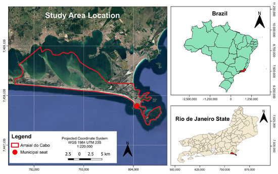
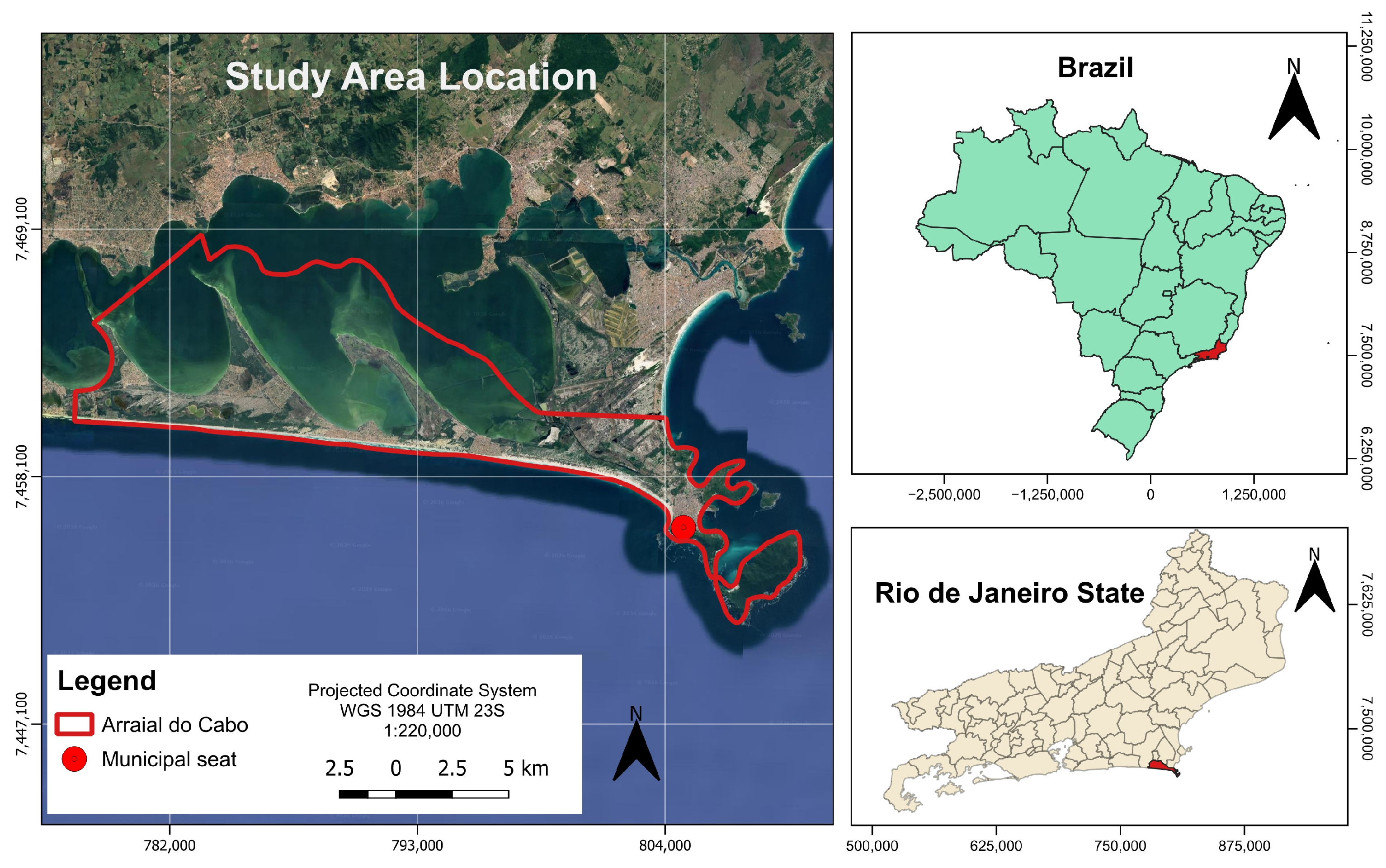
The theme of this study was the LST and LC changes in the municipality of Arraial do Cabo (Figure 1) in the Rio de Janeiro State’s Lake Region due to urban expansion and the degradation of native sandbanks [20,21,23,24]. Arraial do Cabo has a total area of 152.106 km2 [22].
Figure 1.
Location of the study area.
2.2. Material and Data
The four software programs used for Digital Image Processing were QGIS version 3.2.0 Bonn with the Semi-Automatic Classification Plugin (SCP) version 6.2.2, Google Earth Pro 7.1.8.3036 (free software), ArcGIS version 10.3 and IDRISI Selva version 17.0 (licensed for LABGEO/IGEOG/UERJ).
The vector file of the municipal limits was obtained from the 2010 Population Census [52]. The Landsat 8 satellite data for the summers of 2014 and 2017, with a 10% limit for clouds, were downloaded from Earth Explorer [53] (Table 1). Those are free data.
Table 1.
Images used.
The level-2 images (bands 2 to 7) for t1 and t2 were delivered by e-mail containing surface reflectance (SR) data per pixel. The level-1 images (band 10) were converted to reflectance with atmospheric correction using the dark object subtraction method (DOS1) in SCP version 6.2.2 for QGIS version 3.2.0. Band 10 was converted into satellite brightness temperature in Celsius [54].
The images were obtained by the satellite at 12:46:56 for t1 and at 12:45:38 for t2 (Brasília time: UTC-2 h during daylight savings time); this difference was not considered.
2.3. LST Scenes Generation
The remote sensing images were downloaded for the summer period with little cloud cover between 2011—when Costa do Sol State Park (PECS) was created—and 2018. The park is a full-protection conservation unit under urban expansion pressure.
To generate the LST maps, the methodology presented by Congedo [55] and used by Pastore [24] was applied.
All vector and raster datasets were reprojected to the WGS 84/UTM zone 23S coordinate reference system. Then, Landsat 8 OLI images of bands 2 to 7, t1 and t2, were stacked into GeoTIFF multiband images. For rendering, images were generated with maximum and minimum values, with cutoffs set at 2% and 98%, extended by zooming into a scale of 1:15,000 over the municipality. Band sets were made with automatic settings in SCP version 6.2.2 for Landsat 8 OLI data.
Training areas of LC were created in the SCP version 6.2.2 using the color composition of t1 by delimiting polygons with 15 samples per class, based on prior knowledge of the study area and historical imagery from Google Earth Pro. Class names were defined according to the Technical Manual for Land Use [56] and categorized as follows: exposed soil, salt ponds, sand, urban areas, vegetation, and water. To ensure a robust accuracy assessment, the validation samples were selected entirely independent of the training dataset. For the classification procedure, the Minimum Distance algorithm was applied. This classifier was ultimately chosen after preliminary visual inspections comparing it against other methods, such as Maximum Likelihood. The Minimum Distance approach yielded more consistent spatial delineation and fewer visual artifacts for this highly specific and heterogeneous coastal landscape.
The images from band 10 were converted to satellite brightness temperature in Celsius, and the LST was calculated [54]. Initially, natural thermal breaks were automatically calculated by the SCP version 6.2.2 for t1 (17.0–21.7; 21.7–26.3; 26.3–31.0 °C) and t2 (19.0–24.0; 24.0–29.0; 29.0–34.0 °C). However, to enable an absolute temporal comparison between t1, t2, and the 2030 projection, dynamic scene-specific intervals could not be used, as they would only represent relative temperature distributions within each specific date. Therefore, fixed thresholds were established to reclassify the images into three standardized classes: ‘coolness’ (≤22.0 °C), ‘medium’ (22.1 °C to 28.0 °C), and ‘heat’ (>28.0 °C). These fixed thresholds were derived from the automated intervals to serve as a constant thermal baseline: 22.0 °C encompasses the lower boundary of the initial medium classes, while 28.0 °C serves as an intermediate benchmark between the upper bounds of t1 and t2. Using these standardized thresholds guarantees that spatial shifts in the ‘heat’ or ‘coolness’ classes represent actual absolute temperature changes on the land surface over time, establishing a consistent basis for the 2030 projection. While the use of absolute temperature thresholds across different dates does not normalize background atmospheric bias—a known limitation in single-day snapshot comparisons—these fixed values were deliberately maintained to perform a sensitivity test of the Markov model against unnormalized, extreme observational states. This approach highlights the model’s response to high-amplitude thermal variations, serving as a preliminary step before the implementation of relative normalization techniques (such as Z-scores) in future long-term studies.
Although the standard thermal remote sensing literature generally refers to these intervals as low, moderate, and high LST, this study retains the operational GIS labels (‘coolness’, ‘medium’, and ‘heat’) throughout the text and spatial modeling outputs for methodological consistency.
To retrieve the LST, the thermal data (band 10) was first converted from Digital Numbers to Top of Atmosphere spectral radiance, and subsequently to At-Satellite Brightness Temperature, using the standard algorithms embedded in the SCP version 6.2.2 plugin based on the thermal constants provided in the image metadata. The final LST was calculated using the following Equation (1):
where
- λ is the wavelength of emitted radiance (10.8 µm for Landsat 8 band 10);
- ρ = 1.438 × 10⁻² m K;
- ε is the land surface emissivity.
The emissivity values were estimated for each land cover class. According to Ref. [24], an emissivity value of 0.90 was attributed to the sand class; 0.94 to the urban area, salt ponds, and exposed soil classes; and 0.98 to the vegetation and water classes.
LST rasters were reclassified considering the class intervals. Then, reclassified rasters were converted into shapefiles and a text column was included in the attribute table of each scene vector to add LST class names. The lowest interval was called coolness, the mean was called medium, and the highest was called heat. The images of the surface temperatures were clipped with the Arraial do Cabo boundaries. The scene shapefiles were dissolved for the LST class name in ArcGIS 10.3.
2.4. LST Transition and Projection
To evaluate changes and generate scenarios, we applied a methodology proposed by Ref. [27] and improved by Ref. [28] in IDRISI Selva version 17.0.
The Arraial do Cabo’s vectors of LST maps were converted to raster images using the RasterVector tool. This process required the input of the total number of rows and columns, which were calculated using Equation (2):
where
(Xmax − Xmin)/resolution
- Xmax is the maximum coordinate value of the bounding box;
- Xmin is the minimum coordinate value of the bounding box;
- Resolution is the spatial resolution used for the grid (100 m, according to the thermal band characteristics of the Landsat 8 satellite).
Finally, the values added to the rows and columns were rounded up to whole numbers, ensuring no decimal places in any of the scenes.
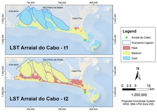
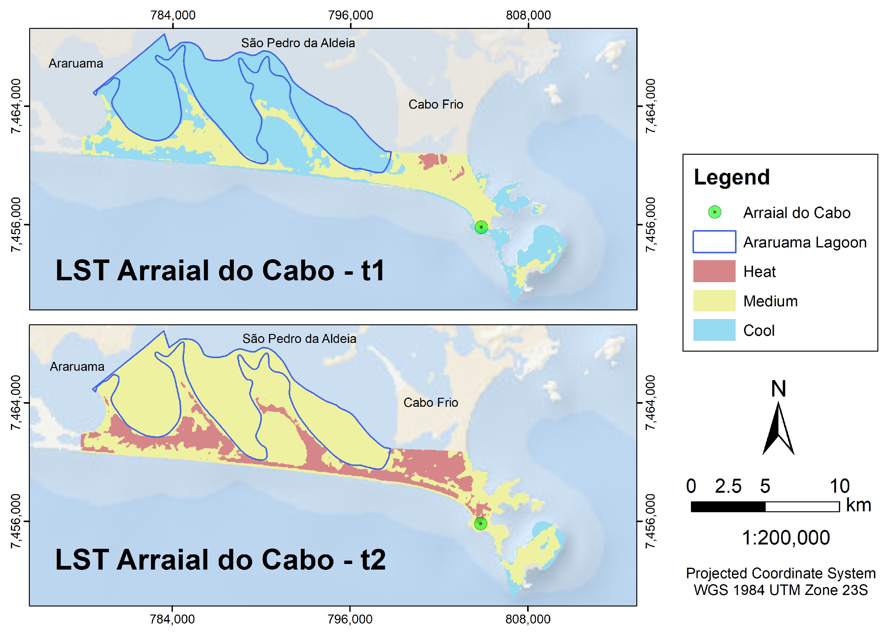
The LST maps were verified in IDRISI Selva version 17.0 to confirm if LST classes from 2014 and 2017 were represented by the same number. In this study, the FID sequences were equal, with 1 representing heat; 2, coolness; and 3, medium (Figure 2).
Figure 2.
LST maps for 2014 (higher) and 2017 (lower).
The area of each class was calculated with the Area tool in IDRISI Selva version 17.0. The transition and prediction were estimated with the Change Analysis tab, Change Demand Modeling and Markov chain functions in LCM. It is important to point out that the estimated prediction for 2030 assumed that the pattern of LST class transitions observed between 2014 and 2017 would remain unchanged, and it does not represent a solid long-term forecast.
To assess the changes in LC classes, their respective percentages were calculated in Excel for 2014 and 2017. The methodology to estimate the transition of classes was reapplied.
The changes in the percentages of LC classes with the highest and lowest emissivity were analyzed, and this factor was used to calculate surface temperature.
3. Results and Discussion
3.1. Spatiotemporal Distribution and Dynamics of Land Surface Temperature (LST)
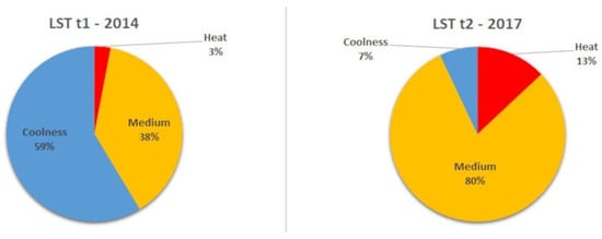
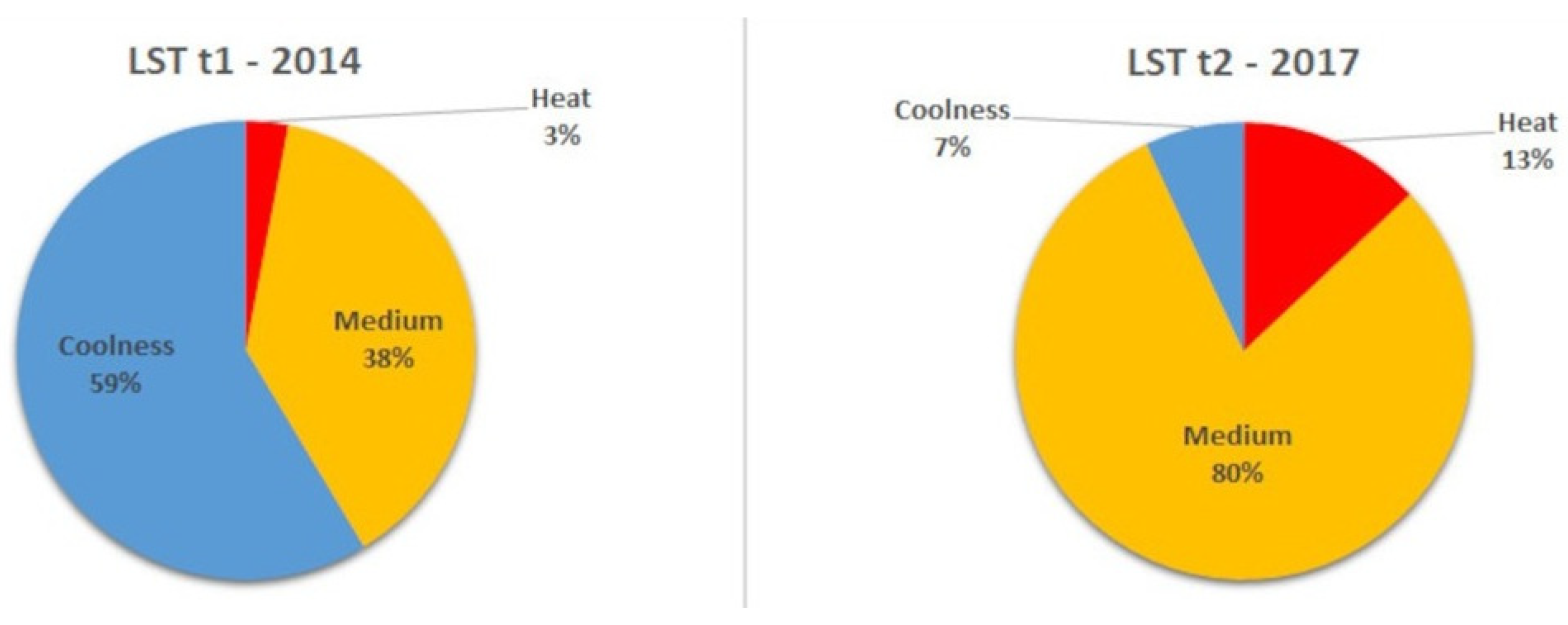
The percentages of each LST class for 2014 and 2017 are shown in Figure 3. While the heat class increased from 3.0% in 2014 to 13.0% in 2017, the coolness class, which was the most frequent class in the 2014 scene with 58.6%, decreased to 7.0% in 2017. The medium class changed from 38.4% in 2014 to 80.0% in 2017.
Figure 3.
Representativeness of the LST classes in 2014 and 2017.
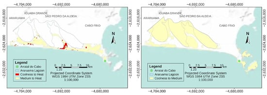
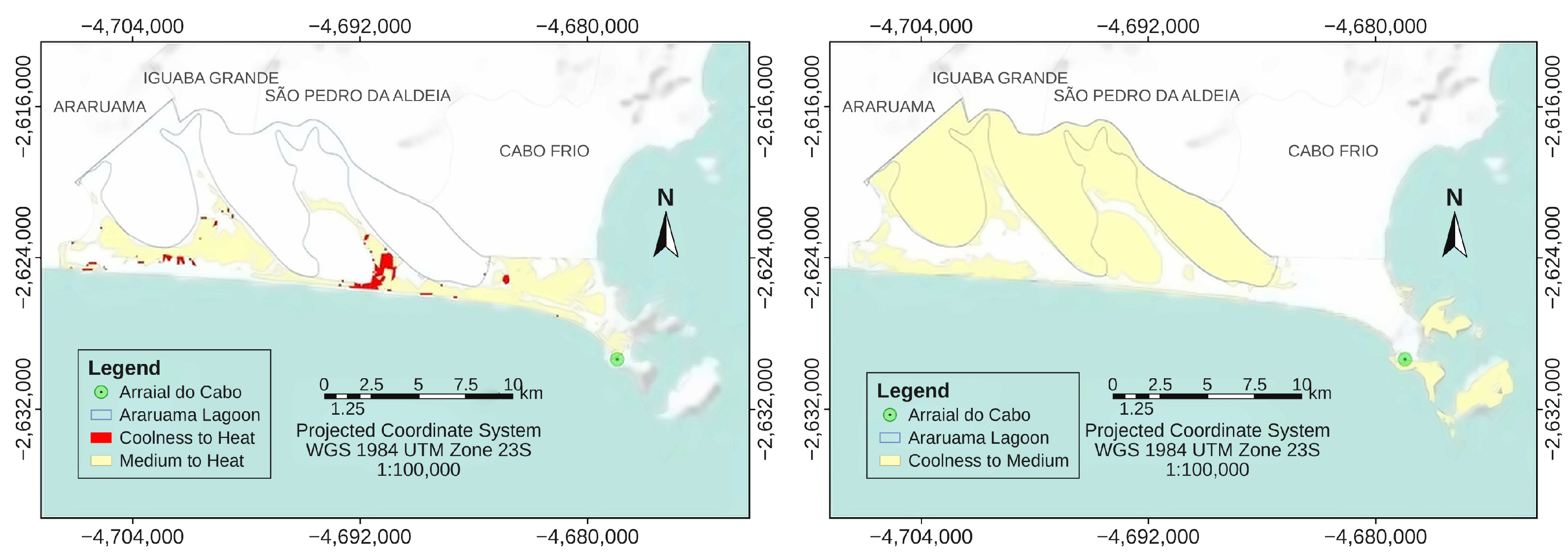
The graphic in Figure 4 shows each class’s losses and gains. While the heat class exclusively expanded, the coolness class exclusively contracted. Medium class gains were three times greater than the losses. Figure 5 shows increases in the areas of the heat and medium classes.
Figure 4.
Graphic of the LST gains and losses in km2.
Figure 5.
Transitions from coolness and medium to heat (left) and from coolness to medium (right).
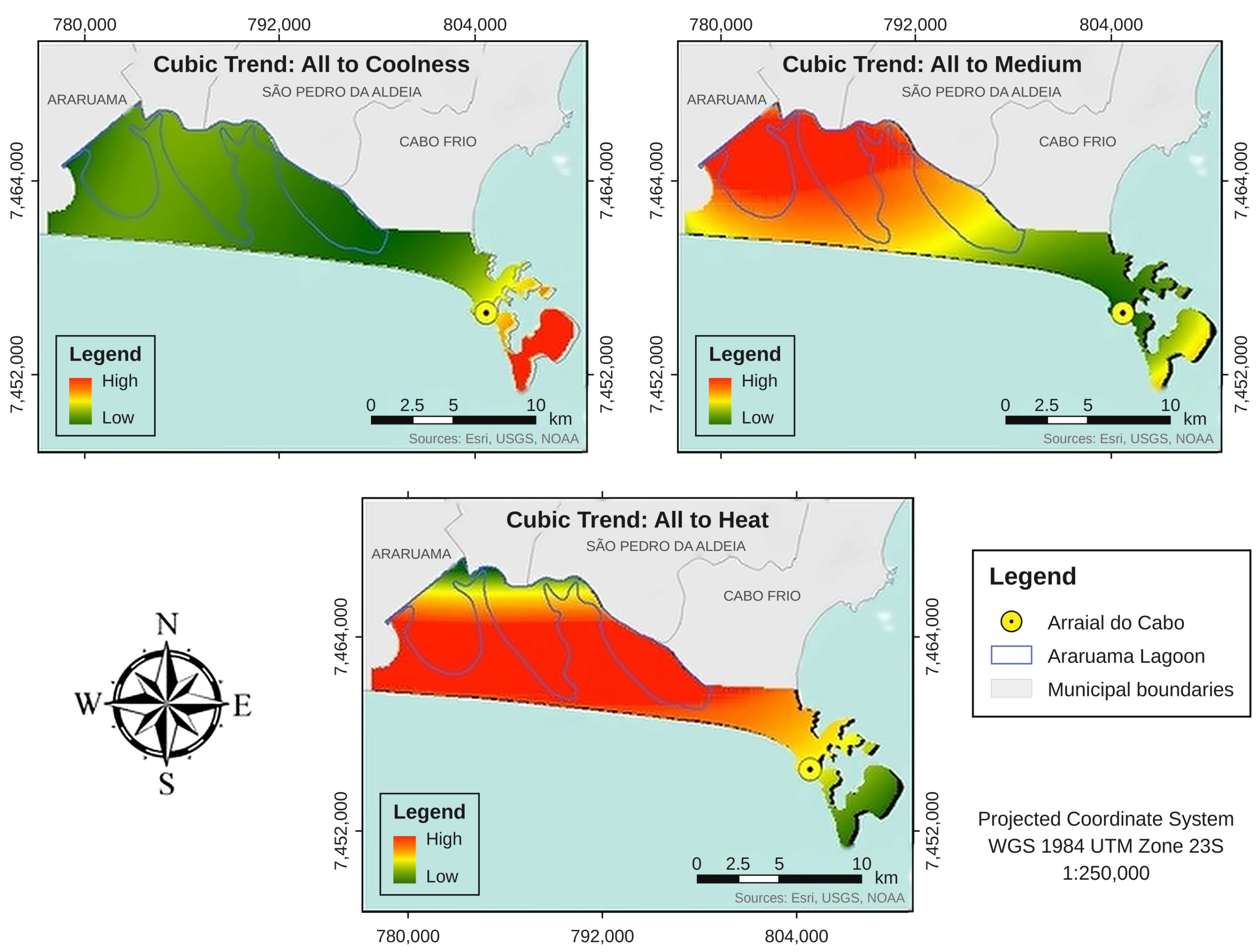
The cubic trend maps for the LST classes are presented in Figure 6. For the largest class of surface temperature (heat), there was an expansion trend for the entire territory of Arraial do Cabo, especially in the area between the lagoon and the ocean, where urban expansion had already been observed [23,24]. The medium class had the highest increase in Araruama Lagoon’s water surface.
Figure 6.
Classes’ cubic trends.
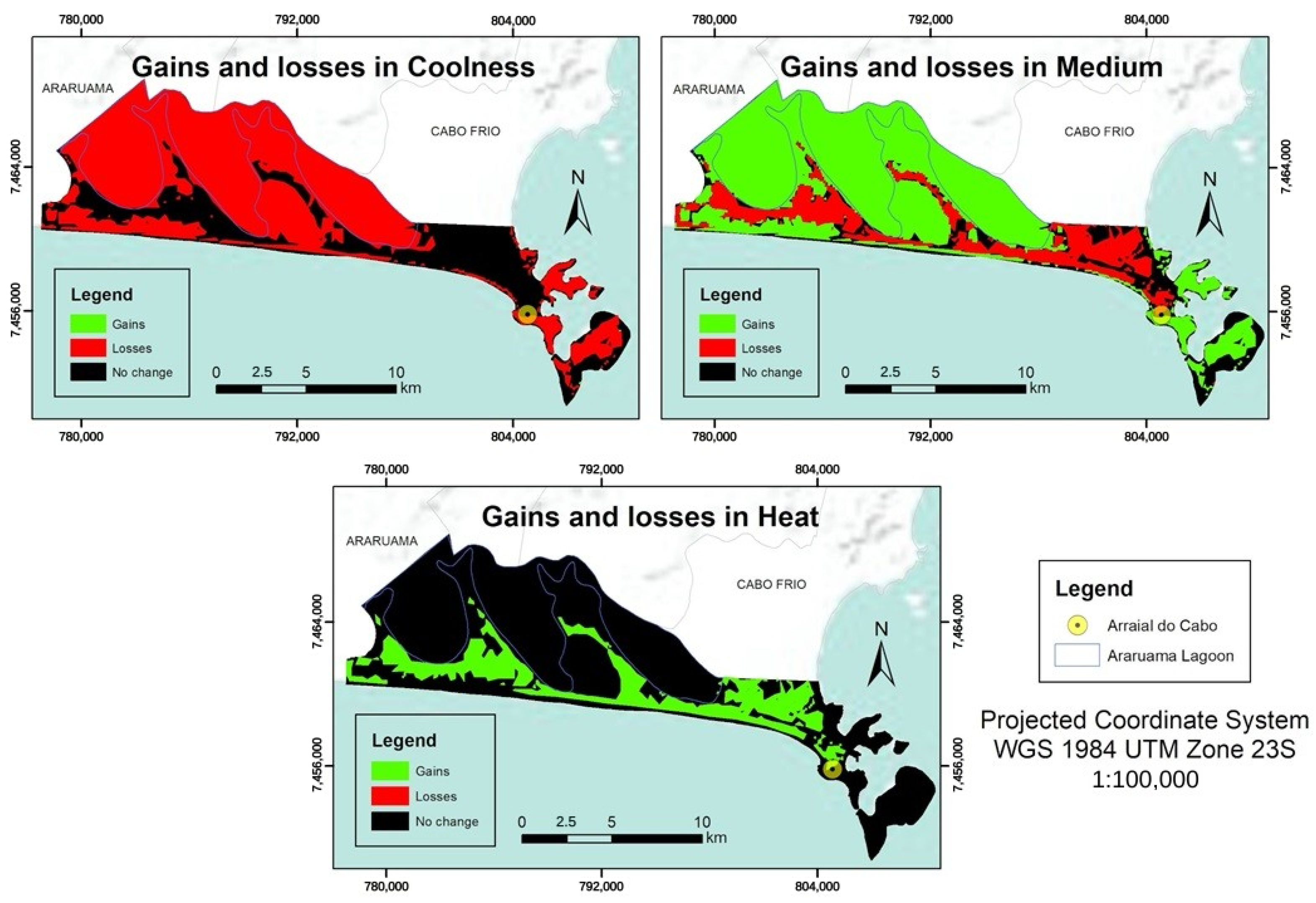
Figure 7 shows the losses and gains of each class of LST.
Figure 7.
LST’s losses and gains.
3.2. Quantitative LST Transition Scenarios for 2030 and Meteorological Context
The quantitative scenario of the LST trend was estimated in IDRISI’s LCM by generating the Markov matrix for the year 2030 (Table 2).
Table 2.
Markov matrix of the quantitative trends of the LST for 2030.
Considering the Markov matrix for 2030, the quantitative trends that most express the probability of a transition occurring between classes are 96.9% (coolness to heat) and 98.9% (medium to heat). The matrix also indicated a 3.1% probability of transition from coolness to medium and a 1.1% probability of the medium class not changing.
The surface temperature trend estimated for 2030 indicated an expansion of the heat class, which would represent more than 90% of Arraial do Cabo. It is worth highlighting that this study used only two images to estimate surface heat, not considering other variables that are essential to elaborate scenarios that are closer to reality. Moreover, 2017 was one of the three warmest years of the planet since 1880 [25], with differences of up to 1.2 °C between the measures obtained at 12:00 and 13:00 in the days of the images (Table 3), according to meteorological data from the automatic station of Arraial do Cabo [57], which can influence surface temperature.
Table 3.
Air temperature differences between t2 and t1.
The mean daily values of the air temperature of the environmental scenes were estimated with the equation proposed by Brazil’s National Meteorology Institute [58] (Table 4).
Table 4.
Values used to calculate the mean air temperature.
Despite the 2.1 °C decrease of the mean daily temperature between t1 and t2, the mean annual temperature using the instantaneous values was 23.0 °C in both cases.
3.3. Land Cover (LC) Classification and Spectral Accuracy Assessment
The LC classifications were validated by estimating their Kappa index [59,60]. The overall accuracy of the classification was estimated by dividing the total number of correctly classified pixels (the sum of the diagonal elements of the confusion matrix) by the total number of reference validation pixels. The values obtained were 94.7% for t1 (Table 5) and 89.4% for 2017 (Table 6), indicating an almost perfect agreement.
Table 5.
Confusion matrix and accuracy assessment for land cover classification in 2014 (t1).
Table 6.
Confusion matrix and accuracy assessment for land cover classification in 2017 (t2).
Despite the overall high agreement in the LC classifications, a closer examination of the confusion matrices reveals specific limitations regarding producer accuracy for certain classes. This lower accuracy is primarily driven by the complex spectral confusion inherent to the physical characteristics of this coastal environment. For instance, dry sand is frequently confused with exposed soil and bright impervious urban surfaces, whereas the spectral signature of salt ponds fluctuates significantly depending on the water level and salt concentration at the exact time of image acquisition. Furthermore, the urban area class showed errors of omission and commission due to the stacking of commercial and residential areas with other land covers. We acknowledge that these spectral overlaps introduce a degree of uncertainty into the transition probabilities calculated by the LCM. Consequently, these inherent classification constraints must be carefully considered when interpreting the 2030 future projection scenarios.
The Kappa hat classification index had a substantial agreement for t1 (0.7) and a moderate agreement for t2 (0.5), according to Bogoliubova and Tymków [61]. These values were influenced by the samples generated as polygons that encompassed different covers and were characterized as the same class. The land cover vectors had a value of 0 for the space between the classified area and the respective rectangle around it. To remove the area outside of the city, the vectors were edited to exclude rows with a value of 0, and as a result, we obtained classifications for the city limits.
3.4. Land Cover Transition Dynamics and Markov Projections
LC changes occurred in 21.5 km2 (13.7% of Arraial do Cabo). An increase occurred in the urban area (which exhibits the lowest emissivity captured by the sensor) as well as in green and sand areas (which exhibit the highest emissivity), potentially influencing LST. Moreover, exposed soil and water (both low-emissivity classes) decreased, but there were no decreases in high-emissivity areas.
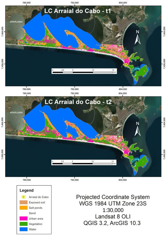
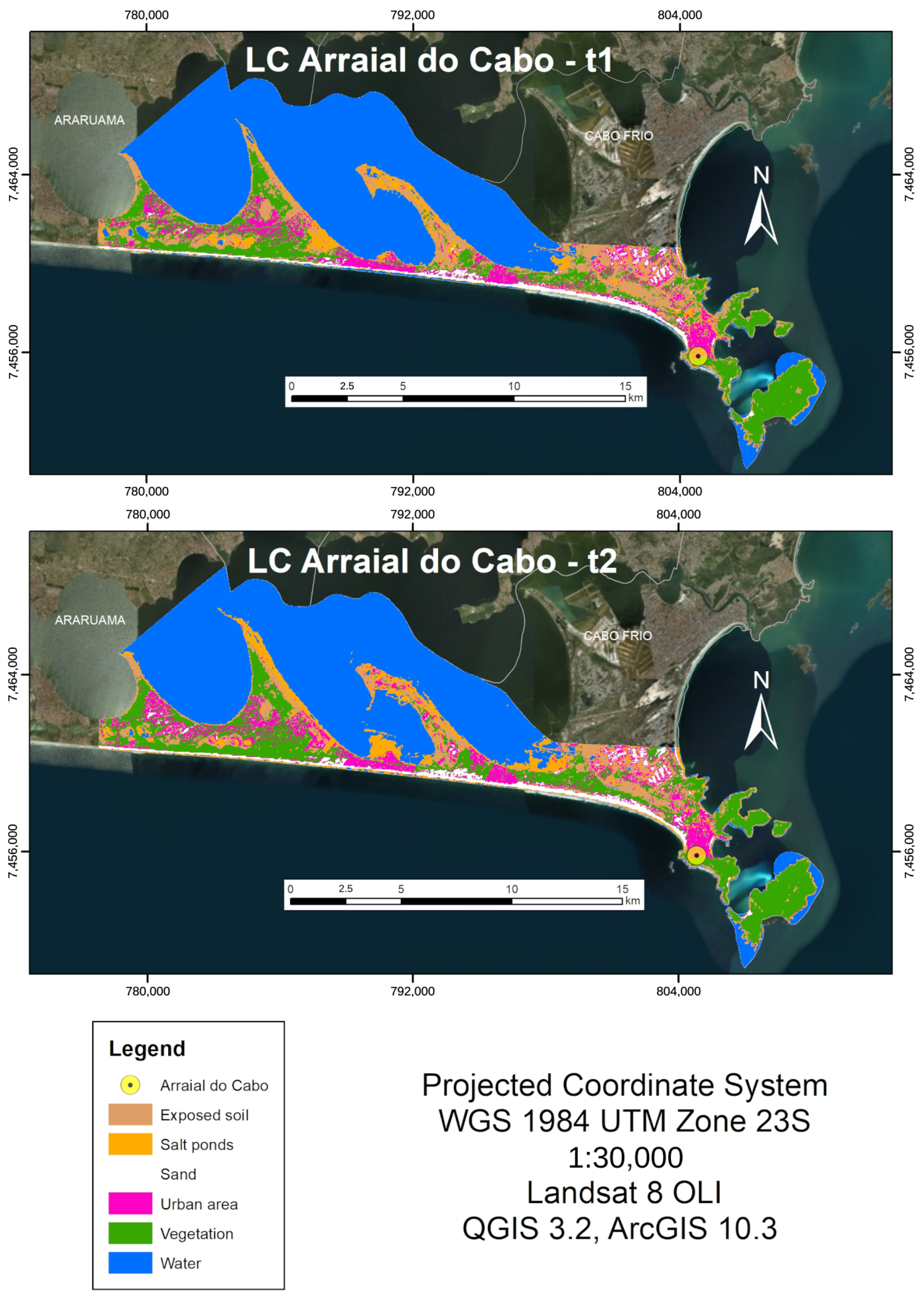
The distribution of land cover classes in t1 and t2 is shown in Figure 8.
Figure 8.
Arraial do Cabo’s LC at t1 and t2.
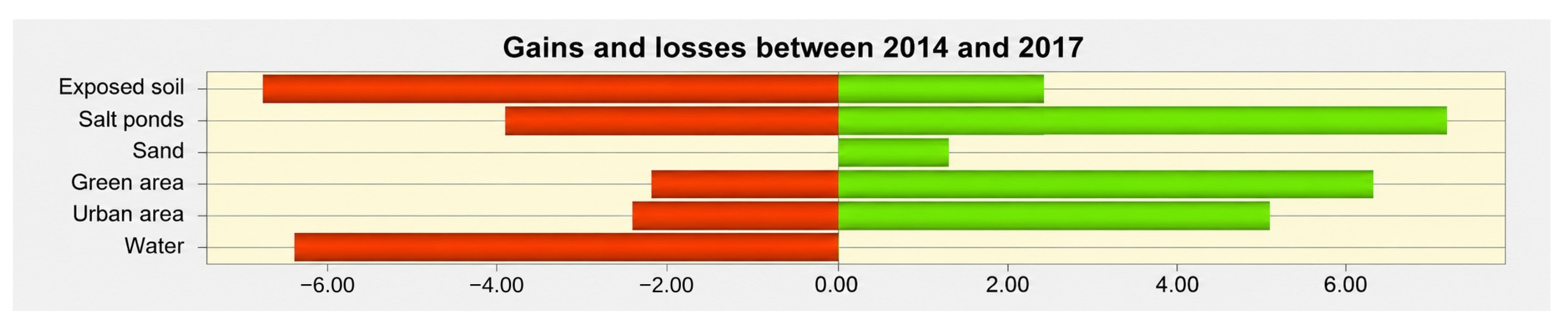
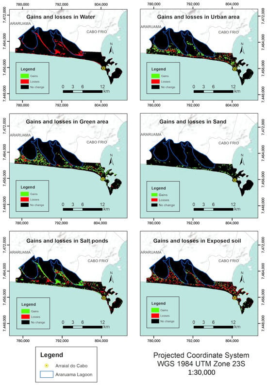
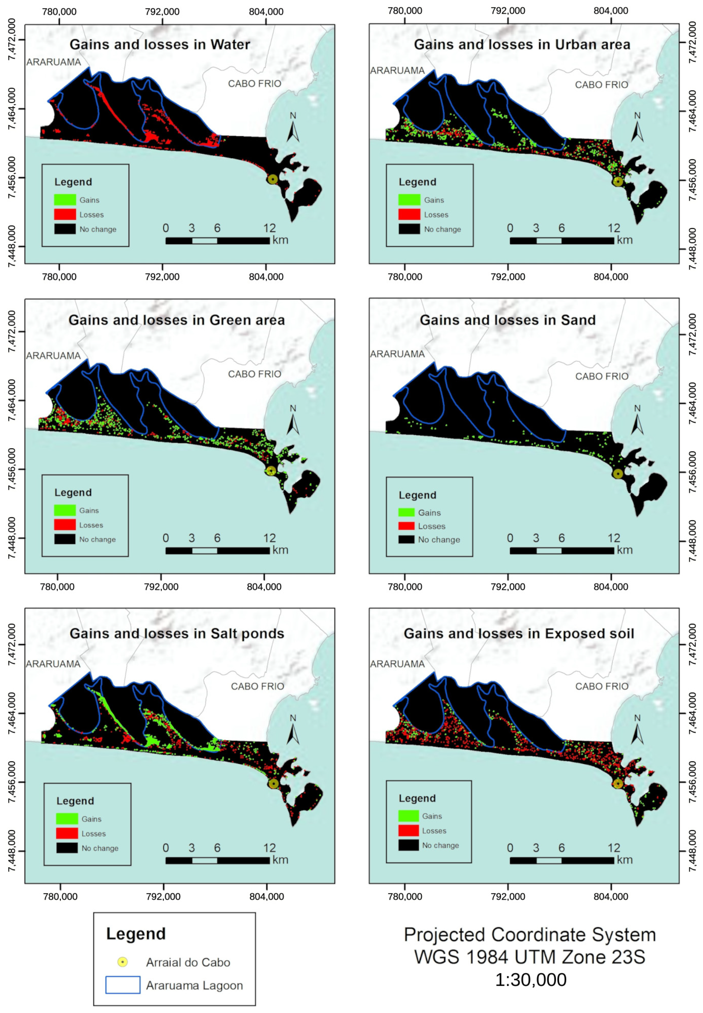
The estimated land cover changes of Arraial do Cabo between 2014 and 2017 were as follows: increase of urban area from 7.4% to 8.9% of the total area of the municipality; green area increasing from 16.2% to 18.7%; sand increase from 2.9% to 3.7%; salt pond increase from 5.8% to 7.6%. Moreover, two classes lost areas: water (56.0% to 52.1%) and exposed soil (11.7% to 9.0%). Some classes showed both gains and losses of areas, while others had only a decrease or increase (Figure 9).
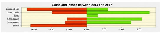
Figure 9.
Graphic of LC’s gains and losses in km2.
Urban area, green area, salt ponds and exposed soil had both gains and losses at t2, and the increase in salt ponds stands out. Exposed soil and water were the classes with the greatest area reduction. The water class showed only decreases, which could be related to the urban expansion close to the lagoon, which has replaced the swamps of the lagoon complex with impervious surfaces, constructions, and exposed soil [20,21,23,24,43]. Figure 10 shows estimated changes for each class.
Figure 10.
LC’s gains and losses.
The urban area grew more than it decreased, expansion occurred more in the western and central areas. The green area had both gains and losses, especially in the east and west of the municipality, and some of its changes were the opposite from those in urban areas.
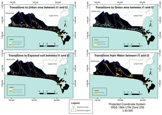
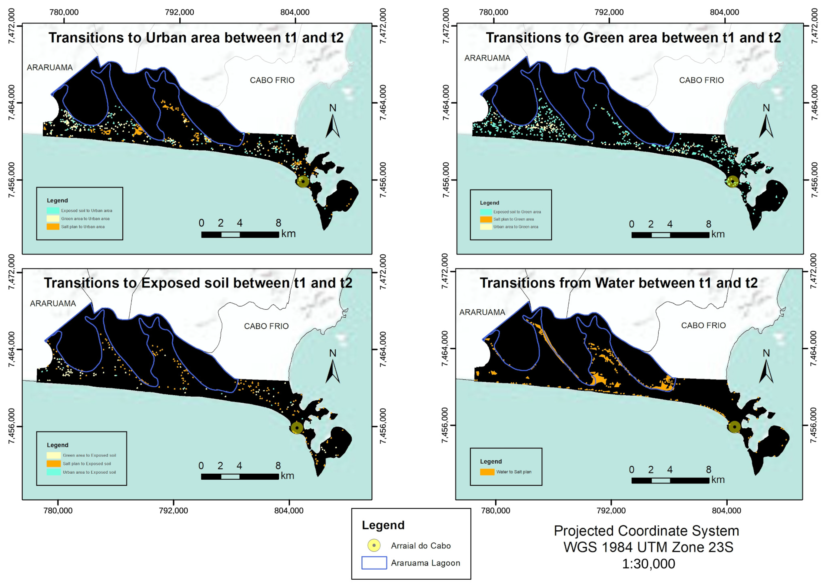
As Figure 11 shows, the area of the sand class only increased, especially close to the sea. The area of the salt ponds showed more gains than losses close to the lagoon. Lastly, the area of exposed soil increased in some locations, but it decreased when the entire area of study is considered. Figure 12 shows the transitions of the LC classes.
Figure 11.
Transitions of the LC classes.
Figure 12.
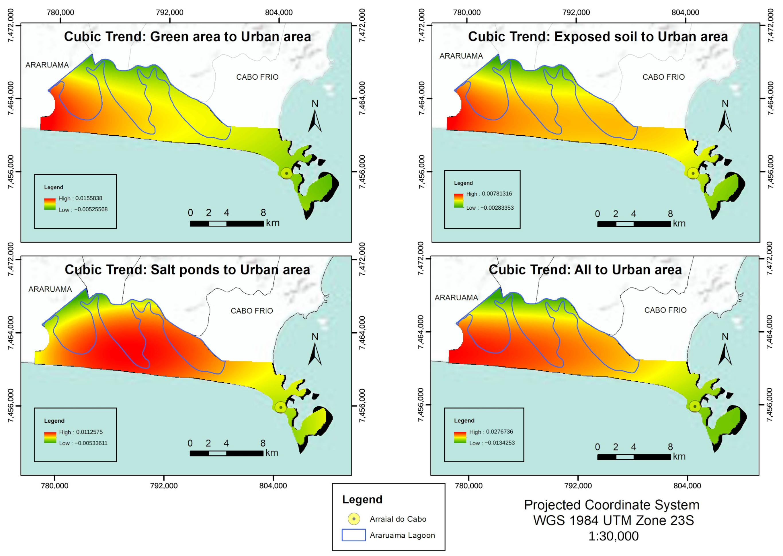
Cubic trend maps of LC classes and all urban areas.
The expansion of the estimated urban area happened mostly in salt ponds and green areas between t1 and t2. The change of green covers to constructed surfaces may increase the LST, and the surface temperature values of the salt ponds were close to urban areas.
The green area class increased mostly where exposed soil decreased, possibly in abandoned construction sites. The water class only decreased where salt ponds increased, which could be related to local climate—in warmer years and days, it could have stimulated evaporation. Moreover, the urban area expanded into salt ponds, causing a different geomorphological process that should be considered in future studies. Figure 12 shows the urban area expansion trend.
3.5. Socioecological Implications for Coastal Sustainability
Urban expansion predominantly occurred in zones that subsequently exhibited gains in moderate and high LST. This correlation suggests that the substitution of natural surfaces increases susceptibility to surface heat accumulation, compounded by anthropogenic activities. As a result, there are concerns about the degradation of the Massambaba sandbank, which is the native ecosystem [21], and the Araruama Lagoon, which is considered the largest permanent hypersaline lagoon worldwide [62].
Furthermore, land-use changes significantly affect adjacent aquatic environments. The replacement of vegetated surfaces with impervious urban areas alters surface runoff, carrying heat and pollutants directly into water bodies. This process can elevate water temperatures and disrupt local hydrological processes, compounding the environmental stress on coastal ecosystems [63].
The quantitative trends of the land cover scenarios for Arraial do Cabo in 2030 are shown in the Markov matrix at Table 7.
Table 7.
Markov matrix of the LC trends for 2030.
The Markov matrix indicated that only the sand class should remain unchanged until 2030. The water surfaces showed a 72.9% probability of remaining unchanged, with a 12.8% chance to change into salt ponds.
The urban area showed probabilities of changing to the sand class (28.8%) and green area (28.7%). The green area had a 73.6% probability of not changing until 2030, and 17.0% of changing into urban area.
The salt pond class showed the most changes. The exposed soil had a 56.2% probability of becoming green area and 18.7% probability of becoming urban area.
Despite the increasing trend for green areas, urban expansion has been observed in the municipality, and it should replace high emissivity surfaces, possibly influencing the LST.
The unilateral expansion of urban areas over salt ponds and native resting vegetation not only triggers local warming but directly threatens the environmental sustainability of the Massambaba sandbank and the Araruama Lagoon complex. These coastal ecosystems provide vital regulating services (such as microclimate stabilization and runoff control), making their preservation a core requirement for local socioecological sustainability.
While spatial overlap is observed between urban expansion and higher LST classes, land cover transformation acts as a contributing factor alongside background daily meteorological variations, such as differences in ambient air temperature between satellite acquisition dates. Therefore, thermal shifts reflect a combination of surface changes and atmospheric conditions rather than a single deterministic driver.
3.6. Limitations and Future Directions
The results presented in this study should be interpreted as a preliminary conditional scenario rather than a robust long-term prediction. The 2030 projection is heavily dependent on the transition matrix derived from a single, high-contrast temporal interval (2014–2017), which included one of the hottest years on record. Consequently, the projected dominance of the ‘heat’ class overestimates long-term reality by propagating a short-term extreme anomaly.
This preliminary assessment establishes the foundational need for more complex methodologies. Future research should enhance this model by:
- Incorporating multi-year time-series data using cloud-computing platforms like Google Earth Engine (GEE) to calculate average summer LST over wider periods (e.g., 2015–2020 and 2020–2025), thereby mitigating the impact of daily meteorological anomalies;
- Integrating actual LST data from 2020 onwards to empirically validate the accuracy of the Markov predictions;
- Applying relative thermal thresholds (e.g., standard deviations or Z-scores) to normalize LST anomalies against background atmospheric temperatures;
- Conducting transition-based quantitative analyses (e.g., specific thermal impacts of vegetation-to-urban transitions) to definitively isolate the effect of land-cover change from meteorological variance.
- Comparing projected LST trends against the Shared Socioeconomic Pathways (SSPs) provided by the CMIP6 framework to verify if the local conditional scenarios align with broader global climate models.
4. Conclusions
The most frequent transitions between t1 and t2 were those from a lower LST to a higher LST, indicating possible locations of high air temperature close to the surface. As for the probability of surface heat accumulation areas being formed, it is important to highlight that the area of study is a coastal valley in which winds disperse surface heat.
In addition to surface temperature, other factors influence air temperature and bioclimatic phenomena, which can vary between t1 and t2. In addition, the replacement of water areas by salt ponds between t1 and t2 indicates that new studies should be performed considering climate monitoring on a local and regional level.
The projection of the surface temperature for 2030 enabled us to estimate the evolution of the heat accumulation on the surface, which was analyzed together with the changes in LC. The increasing trend of the classes with a higher LST and of urban areas serve as a warning about the negative environmental impacts on the native ecosystem, the local state park, Araruama Lagoon, and the land surface of the studied municipality.
The data suggest that the increase of urban surfaces is a contributing factor to localized thermal changes. However, further transition-specific quantitative analyses are required to definitively establish urbanization as the dominant driver over meteorological variance. If there is a proper conservation of the state park, its surroundings, and Araruama Lagoon, it is possible for the green areas to expand or not be altered until 2030.
The level-2 Landsat 8 images show differences that shorten the pre-processing of the images, such as the conversion to surface reflectance. In this study, level-1 and level-2 images were not compared.
It is worth highlighting that the results were generated based on estimates about satellite images from two instants in different years, with different meteorological conditions. The application of this methodology may consider temporal series data and other periods and combine with other environmental scenes to indicate trends and alternative scenarios, and the results may be applied in environmental and territorial planning to increase sustainability in coastal areas.
In summary, this study demonstrates that integrating spatiotemporal monitoring of land surface temperature and land cover is not merely a technical exercise but a fundamental sustainability tool for vulnerable coastal territories. By bridging microclimatic dynamics with predictive Markov modeling, our exploratory analysis underscores that maintaining the ecological sustainability of coastal environments—such as the restinga vegetation of Massambaba and the hypersaline Araruama Lagoon—is intrinsically linked to managing local thermal resilience. Ultimately, these preliminary scenarios provide actionable, diagnostic baselines that can guide decision-makers in formulating integrative territorial planning policies. It is through such proactive, science-grounded spatial governance that coastal municipalities can mitigate microclimatic degradation, foster urban thermal resilience, and translate global sustainable development goals into localized, long-term environmental sustainability.
Author Contributions
Conceptualization, V.O.P. and L.A.B.d.D.; Methodology, V.O.P., L.A.B.d.D. and A.C.d.S.O.J.; Formal analysis, V.O.P., L.A.B.d.D., V.C.d.C., A.C.d.S.O.J., M.A.V.d.F. and N.F.d.S.; Investigation, V.O.P. and L.A.B.d.D.; Resources, M.A.V.d.F. and N.F.d.S.; Writing—original draft, V.O.P., L.A.B.d.D. and A.C.d.S.O.J.; Writing—review and editing, V.C.d.C., M.A.V.d.F. and N.F.d.S.; Supervision, L.A.B.d.D., V.C.d.C., M.A.V.d.F. and N.F.d.S. All authors have read and agreed to the published version of the manuscript.
Funding
This research received no external funding.
Institutional Review Board Statement
Not applicable.
Informed Consent Statement
Not applicable.
Data Availability Statement
The original contributions presented in this study are included in the article. Further inquiries can be directed to the corresponding authors.
Conflicts of Interest
The authors declare no conflicts of interest.
References
- Grimmond, C.S.B. Progress in measuring and observing the urban atmosphere. Theor. Appl. Climatol. 2006, 84, 3–22. [Google Scholar] [CrossRef] [Scilit]
- Kanda, M. Progress in urban meteorology: A review. J. Meteorol. Soc. Jpn. 2007, 85B, 363–383. [Google Scholar] [CrossRef] [Scilit]
- Voogt, J.A.; Oke, T.R. Thermal remote sensing of urban climates. Remote Sens. Environ. 2003, 86, 370–384. [Google Scholar] [CrossRef] [Scilit]
- Arnfield, A.J. Two decades of urban climate research: A review of turbulence, exchanges of energy and water, and the urban heat island. Int. J. Climatol. 2003, 23, 1–26. [Google Scholar] [CrossRef] [Scilit]
- Ren, C.; Ng, E.Y.; Katzschner, L. Urban climatic map studies: A review. Int. J. Climatol. 2001, 31, 2213–2233. [Google Scholar] [CrossRef] [Scilit]
- Gallego, L.P. Tipos de Tempo e Poluição Atmosférica no Rio de Janeiro: Um Ensaio em Climatologia Urbana. Ph.D. Thesis, Universidade de São Paulo, São Paulo, Brazil, 1972. [Google Scholar]
- Brandão, A.M.P.M. Tendências e Oscilações Climáticas na Área Metropolitana do Rio de Janeiro. Master’s Thesis, Universidade de São Paulo, São Paulo, Brazil, 1987. [Google Scholar]
- Brandão, A.M.P.M. Clima Urbano da Cidade do Rio de Janeiro. Ph.D. Thesis, Universidade de São Paulo, São Paulo, Brazil, 1996. [Google Scholar]
- Brandão, A.M.P.M. Clima urbano e as enchentes na cidade do Rio de Janeiro. In Impactos Ambientais Urbanos, 1st ed.; Guerra, A.J.T., Cunha, S.B., Eds.; Bertrand Brasil: Rio de Janeiro, Brazil, 2001; Volume 1, pp. 47–109. [Google Scholar]
- Fialho, E.S. Análise Temporoespacial do Campo Térmico na Ilha do Governador/RJ em Episódios de Verão e Inverno. Master’s Thesis, Universidade Federal do Rio de Janeiro, Rio de Janeiro, Brazil, 2002. [Google Scholar]
- Lucena, A.J. O Clima de Bangu no Contexto do Clima Urbano da Cidade do Rio de Janeiro. Bachelor’s Thesis, Universidade Federal do Rio de Janeiro, Rio de Janeiro, Brazil, 2002. [Google Scholar]
- Marques Filho, E.P.; Karam, H.A.; Miranda, A.G.; França, J.R.A. Rio de Janeiro’s tropical urban climate. Q. Newsl. Int. Assoc. Urban Clim. 2009, 32, 5–9. [Google Scholar]
- Karam, H.A.; Pereira Filho, A.J.; Masson, V.; Noilhan, J.; Marques Filho, E.P. Formulation of a tropical town energy budget (t-TEB) scheme. Theor. Appl. Climatol. 2010, 101, 109–120. [Google Scholar] [CrossRef] [Scilit]
- Cui, L.; Shi, J. Urbanization and its environmental effects in Shanghai, China. Urban Clim. 2012, 2, 1–15. [Google Scholar] [CrossRef] [Scilit]
- Pacifici, M.; Rama, F.; Marins, K.R.C. Analysis of temperature variability within outdoor urban spaces at multiple scales. Urban Clim. 2019, 27, 90–104. [Google Scholar] [CrossRef] [Scilit]
- Ferreira, L.S.; Duarte, D.H.S. Exploring the relationship between urban form, land surface temperature and vegetation indices in a subtropical megacity. Urban Clim. 2019, 27, 105–123. [Google Scholar] [CrossRef] [Scilit]
- Katzschner, L.; Freire, T.M.M.; Andrade, T.C.Q.; Carvalho, M.L.; Nery, J.F.G. Urban climate study of Salvador: Thermal comfort pattern. In Proceedings of the ENCAC 1999, Salvador, Brazil, 22–26 November 1999. [Google Scholar]
- Tarifa, J.R.; Armani, G. Unidades Climáticas Urbanas na cidade de São Paulo, 1a aproximação. In Relatório Preliminar do Projeto Atlas Ambiental do Município de São Paulo; Relatório Interno; PMSP/SVMA: São Paulo, Brazil, 2000. [Google Scholar]
- Sousa, S.B.; Ferreira, L.G. Análise da temperatura de superfície em ambientes urbanos: Um estudo por meio de sensoriamento remoto no município de Goiânia, Goiás (2002–2011). Confins 2012, 15, 2012. [Google Scholar] [CrossRef] [Scilit]
- Azevedo, R.L. Diagnóstico Geossocioambiental e Dinâmicas Territoriais da Região dos Lagos Fluminenses (RJ): Subsídios ao Plano de Manejo do Parque Estadual da Costa do Sol—PECS. Ph.D. Thesis, Universidade do Estado do Rio de Janeiro, Rio de Janeiro, Brazil, 2016. [Google Scholar]
- Bidegain, P.; Pereira, L.F.M. Plano das Bacias Hidrográficas da Região dos Lagos e do Rio São João, 1st ed.; Consórcio Intermunicipal para Gestão das Bacias Hidrográficas da Região dos Lagos, Rio São João e Zona Costeira: Rio de Janeiro, Brazil, 2005. [Google Scholar]
- IBGE Cidades: Brasil—Rio de Janeiro—Arraial do Cabo. Available online: https://cidades.ibge.gov.br/brasil/rj/arraial-do-cabo/panorama (accessed on 31 May 2021).
- Deslandes, R.S. Entre a Lagoa e o Mar: Ordenamento Territorial e Impactos Ambientais na Restinga de Massambaba, Região dos Lagos (RJ). Master’s Thesis, Universidade do Estado do Rio de Janeiro, Rio de Janeiro, Brazil, 2013. [Google Scholar]
- Pastore, V.O. Balanço Hídrico Como Subsídio a Tetos Verdes Para a Conservação da Restinga de Massambaba (Arraial do Cabo), RJ, Brasil. Master’s Thesis, Universidade do Estado do Rio de Janeiro, Rio de Janeiro, Brazil, 2016. [Google Scholar]
- NOAA: 2017 Was 3rd Warmest Year on Record for the Globe. Available online: https://www.noaa.gov/news/noaa-2017-was-3rd-warmest-year-on-record-for-globe (accessed on 15 July 2018).
- UN. Transforming Our World: The 2030 Agenda for Sustainable Development. Available online: https://sustainabledevelopment.un.org/post2015/transformingourworld (accessed on 28 July 2018).
- Eastman, J.R. Idrisi Kilimanjaro, 1st ed.; Clark University: Worcester, MA, USA, 2003. [Google Scholar]
- Beser de Deus, L.A. Espaço e Tempo Como Subsídios à Construção de Cenários de Uso e Cobertura da Terra para o Planejamento Ambiental na Amazônia: O Caso da Bacia do Rio Acre. Ph.D. Thesis, Universidade Federal do Rio de Janeiro, Rio de Janeiro, Brazil, 2013. [Google Scholar]
- Briassoulis, H. Analysis of Land Use Change: Theoretical and Modeling Approaches; Web Book of Regional Science: Morgantown, WV, USA, 2019. [Google Scholar]
- Harvey, D. Models of spatial patterns evolution in Human Geography. In Models in Geography, 1st ed.; Chorley, R.J., Hagget, P., Eds.; EDUSP: São Paulo, Brazil, 1974; Volume 1. [Google Scholar]
- Haykin, S. Neural Networks: Princípios e Prática, 1st ed.; Bookman: Porto Alegre, Brazil, 2001. [Google Scholar]
- Mansilla Baca, J.F. Dinâmica da Paisagem: Métodos Analíticos e Modelos de Classificação e Simulação Prognóstica, Sob a Ótica Geoecológica. Ph.D. Thesis, Universidade Federal do Rio de Janeiro, Rio de Janeiro, Brazil, 2002. [Google Scholar]
- Mansilla Baca, J.F.; Coelho Netto, A.L.; Menezes, P.M.L. Modelagem da Dinâmica da Paisagem com Processos de Markov. In Geomática: Modelos e Aplicações Ambientais, 1st ed.; Meirelles, M.S.P., Camara, G., Almeida, C.C.M., Eds.; Embrapa Informação Tecnológica: Brasília, Brazil, 2007. [Google Scholar]
- Markov, A.A. Extension of the limit theorems of probability theory to a sum of variables connected in a chain. In Dynamic Probabilistic Systems, 1st ed.; Howard, R.A., Ed.; John Wiley and Sons: New York, NY, USA, 1971; Volume 1. [Google Scholar]
- Ruhoff, A.; Fantin-Cruz, I.; Collischonn, W. Modelos de simulação dinâmica do desmatamento na Amazônia. Caminhos Geogr. 2010, 11, 258–268. [Google Scholar] [CrossRef] [Scilit]
- Soares Filho, B. Modelagem da Dinâmica de Paisagem de Uma Região de Fronteira de Colonização Amazônica. Ph.D. Thesis, Universidade de São Paulo, São Paulo, Brazil, 1998. [Google Scholar]
- Tian, H.; Banger, K.; Bo, T.; Dadhwal, V.K. History of land use in India during 1880–2010: Large-scale land transformations reconstructed from satellite data and historical archives. Glob. Planet. Change 2014, 121, 78–88. [Google Scholar] [CrossRef] [Scilit]
- Friehat, T.; Mulugeta, G.; Gala, T.S. Modeling urban sprawls in northeastern Illinois. J. Geosci. Geomat. 2015, 3, 133–141. [Google Scholar]
- Mishra, V.N.; Rai, P.K.; Mohan, K. Prediction of land use changes based on Land Change Modeler (LCM) using remote sensing: A case study of Muzaffarpur (Bihar), India. J. Geogr. Inst. Cvijic 2014, 64, 111–127. [Google Scholar] [CrossRef] [Scilit]
- Mohamed, A.; Worku, H. Simulating urban land use and cover dynamics using cellular automata and Markov chain approach in Addis Ababa and the surrounding. Urban Clim. 2020, 31, 100545. [Google Scholar] [CrossRef] [Scilit]
- Pechanec, V.; Mráz, A.; Benc, A.; Macků, K.; Cudlín, P. Prediction of Land-Use Development Under Influence of Climate Change. In Dynamics in GIscience. GIS OSTRAVA 2017, 1st ed.; Ivan, I., Horák, J., Inspektor, T., Eds.; Lecture Notes in Geoinformation and Cartography; Springer: Cham, Switzerland, 2018; Volume 1. [Google Scholar] [CrossRef] [Scilit]
- Neves, L.V.; Beser de Deus, L.A.; Oscar Júnior, A.C.S.; Fernandes, M.C. Mudanças de uso e cobertura da terra e áreas suscetíveis à inundação—Estudo de caso do município de Duque de Caxias/RJ. Rev. Dep. Geogr. 2019, 37, 30–43. [Google Scholar] [CrossRef] [Scilit]
- Pereira, E.S.; Beser de Deus, L.A.; Ribeiro, M.F.; Costa, V.C. Dinâmica de valorização do solo urbano próximo de unidades de conservação—Estudo de caso do bairro de Campo Grande, município do Rio de Janeiro. Rev. Dep. Geogr. 2021, 41, e169722. [Google Scholar] [CrossRef] [Scilit]
- Baptista, J.V.; Beser de Deus, L.A. Análise espaço-temporal do uso e ocupação do solo no período dos mega eventos esportivos na Bacia Hidrográfica de Jacarepaguá, município do Rio de Janeiro. Humboldt 2021, 1, 3. [Google Scholar]
- Branco, T.L.; Almeida, C.M.; Francisco, C.N. Modelagem dinâmica espacial das mudanças de uso e cobertura da terra na Região Hidrográfica da Baía da Ilha Grande-RJ: Um enfoque sobre comunidades tradicionais e Unidades de Conservação. Rev. Bras. Cartogr. 2022, 74, 137–158. [Google Scholar] [CrossRef] [Scilit]
- Zhou, D.; Xiao, J.; Bonafoni, S.; Berger, C.; Deilami, K.; Zhou, Y.; Frolking, S.; Yao, R.; Qiao, Z.; Sobrino, J.A. Satellite Remote Sensing of surface urban heat islands: Progress, challenges, and perspectives. Remote Sens. 2019, 11, 48. [Google Scholar] [CrossRef] [Scilit]
- Agbor, C.F.; Makinde, E.O. Land surface temperature mapping using geoinformation techniques. Geoinformatics FCE CTU 2018, 17, 17–32. [Google Scholar] [CrossRef] [Scilit]
- Ashraf, M. A study of temporal change in land surface temperature and urban heat island effect in Patna Municipal Corporation over a period of 25 years (1989–2014) using remote sensing and GIS technique. Int. J. Remote Sens. Geosci. 2015, 4, 71–77. [Google Scholar]
- Kumar, K.S.; Bontha, A.D.; Arneepalli, C.K.; Chandrala, M.; Tekumudi, V.P. Study of urban surface temperature changes of Vijayawada City using Remote Sensing and GIS. Int. J. Innov. Res. Adv. Eng. 2015, 2, 98–102. [Google Scholar]
- Zaki, R.; Zaki, A.; Ahmed, S. Land use and land cover changes in arid region: The case new urbanized zone, Northeast Cairo, Egypt. J. Geogr. Inf. Syst. 2011, 3, 173–194. [Google Scholar] [CrossRef]
- Mustafa, E.K. Predicting of Land surface temperature distribution in Freetown City, Sierra Leone by using polynomial curve fitting model. J. Geogr. Inf. Syst. 2020, 12, 531–544. [Google Scholar] [CrossRef]
- IBGE. Geociências. Available online: https://downloads.ibge.gov.br/downloads_geociencias.htm (accessed on 25 July 2018).
- USGS. EarthExplorer. Available online: https://earthexplorer.usgs.gov (accessed on 22 June 2018).
- Congedo, L. Landsat 8 Surface Reflectance: A Comparison of DOS1 Correction and USGS High Level Data Products. Available online: https://fromgistors.blogspot.com/2015/01/landsat-8-surface-reflectance.html (accessed on 5 January 2019).
- Congedo, L. Estimation of Land Surface Temperature with Landsat Thermal Infrared Band: A Tutorial Using the Semi-Automatic Classification Plugin for QGIS. Available online: https://fromgistors.blogspot.com/2014/01/estimation-of-land-surface-temperature.html (accessed on 30 June 2018).
- IBGE. Manual Técnico de Uso da Terra, 3rd ed.; IBGE: Rio de Janeiro, Brazil, 2013. [Google Scholar]
- NAPROA. Dados Meteorológicos da Estação Automática de Arraial do Cabo—INMET A606; Núcleo Aplicado ao Estudo e Processos Oceânicos e Atmosféricos (UERJ): Rio de Janeiro, Brazil, 2019. [Google Scholar]
- INMET. Normais Climatológicas do Brasil: 1961–1990; Instituto Nacional de Meteorologia (INPE): Brasília, Brazil, 2019. [Google Scholar]
- QGISBrasil. Classificação Supervisionada de Imagens Orbitais com o Semi-Automatic Classification Plugin. Available online: https://qgisbrasil.org/2015/08/18/qgis-classificacao-supervisionada-de-imagens-orbitais-com-o-semi-automatic-classification-plugin (accessed on 25 July 2018).
- Vieira, G. Avaliação do Erro de Classificação Uma Imagem de Satélite Usando o QGIS e o SCP. 2016. Available online: https://www.youtube.com/watch?v=k1yjcJPb1WI (accessed on 10 January 2019).
- Bogoliubova, A.; Tymków, P. Accuracy assessment of automatic image processing for land cover classification of St. Petersburg Protected Area. Geod. Descr. Terr. 2014, 13, 5. [Google Scholar]
- Primo, P.B.S.; Bizerril, C.R.S.F. Perfil Ambiental do Maior Ecossistema Lagunar Hipersalino do Mundo, 1st ed.; Secretaria de Estado de Meio Ambiente e Desenvolvimento Sustentável: Rio de Janeiro, Brazil, 2002. [Google Scholar]
- Biedunkova, O.; Kuznietsov, P.; Tsos, O.; Karaim, O. Hydrochemical Typology of Natural Lakes in the Polissia Region Based on Self-Organizing Maps: Implications for Sustainable Water Resources Management. Water 2026, 18, 926. [Google Scholar] [CrossRef] [Scilit]



Disclaimer/Publisher’s Note: The statements, opinions and data contained in all publications are solely those of the individual author(s) and contributor(s) and not of MDPI and/or the editor(s). MDPI and/or the editor(s) disclaim responsibility for any injury to people or property resulting from any ideas, methods, instructions or products referred to in the content. |
© 2026 by the authors. Licensee MDPI, Basel, Switzerland. This article is an open access article distributed under the terms and conditions of the Creative Commons Attribution (CC BY) license.