


Abstract
Lending to small and medium-sized enterprises (SMEs) on the basis of their environmental, social, and governance (ESG) performance is difficult for commercial banks. The data needed for a proper assessment are rarely at hand, and existing tools cannot capture experts’ fuzziness, complex hesitation, and preference characteristics at the same time. This paper introduces the probabilistic picture hesitant fuzzy set (PPHFS) into SME ESG evaluation and develops a multi-attribute group decision-making (MAGDM) method that rests on the correlation coefficient of PPHFSs. The method has three components. It first defines the information energy of PPHFSs, builds a correlation measure on that foundation, and then derives several correlation coefficients together with their weighted forms. A separate procedure converts the multi-dimensional voting information that evaluators provide through questionnaires and balloting into probabilistic picture hesitant fuzzy information, which keeps the approach close to practice. These components are assembled into a complete MAGDM framework for banks and illustrated on a numerical case of five SME loan applicants. Sensitivity analysis and comparative experiments corroborate the feasibility and effectiveness of the method. By aligning bank credit decisions with ESG screening, the framework supports the extension of green credit to SMEs and contributes to sustainable finance and the Sustainable Development Goals (SDGs).
1. Introduction
1.1. Background and Motivation
SMEs form the backbone of China’s economy. They contribute more than 60% of GDP and account for roughly 80% of urban employment, yet chronic financing difficulties continue to slow their growth and innovation. As the country pursues its dual carbon goals and moves toward a greener economy, regulators now expect commercial banks to factor environmental, social, and governance (ESG) considerations into credit decisions. Two aims underlie this expectation: steering capital toward sustainable firms, and containing the credit risk that environmental and social liabilities can create. This lending objective is directly linked to sustainable development: steering credit toward SMEs with sound ESG performance advances inclusive economic growth, responsible industry and innovation, and climate action, in line with the Sustainable Development Goals (SDGs 8, 9, and 13).
In practice, however, the green lending market remains uneven. Large listed companies and state-owned enterprises have standardized disclosure systems and third-party ratings behind them, so green financing is comparatively accessible; SMEs, by contrast, are constrained by expensive disclosure, thin managerial resources, and scarce data, and are often effectively excluded from green credit altogether. When data are missing, banks have no choice but to assess the ESG profile of SME applicants themselves, drawing mainly on expert opinion and qualitative judgment, or what is often called soft information. The problem then becomes a fuzzy multi-attribute decision-making (MADM) task full of uncertainty, hesitation, and divergent expert preferences. We tackle it with the PPHFS and a correlation coefficient-based multi-attribute group decision-making (MAGDM) method designed for SME green lending.
This regulatory context is relevant to SME green lending. In 2012, the Green Credit Guidelines issued by the China Banking and Insurance Regulatory Commission gave banks a first framework for screening environmental and social risk. Eight years later, the Guiding Opinions on Promoting High-Quality Development of Green Finance went a step further and asked that ESG principles run through the entire lending process [1]. Reality, however, has not matched the policy design. Large listed companies and state-owned enterprises, armed with standardized disclosures and third-party rating endorsements, obtain green financing with little difficulty; SMEs, weighed down by disclosure costs and scarce data, remain largely shut out [2].
Regulators have tried to correct this imbalance by pressing banks to lend more to SMEs and by making such lending part of mandatory performance evaluation. Banks therefore have to perform ESG assessments of SME borrowers on their own. In practice these assessments lean heavily on the subjective expertise of risk-control reviewers and relationship managers, and they struggle with the uncertainty inherent in the assessment subjects [3]. Differences among experts in professional background, work experience, and cognitive style add further hesitation and vagueness [3]. To address these challenges, the framework developed below does not eliminate this subjectivity; it organizes and records it, so that expert judgments become structured, transparent, and auditable.
Fuzzy sets have been regarded as a remedy since Zadeh’s seminal 1965 paper [4]. Researchers have introduced a stream of extensions into ESG evaluation, from triangular fuzzy numbers and Z-fuzzy numbers to interval-valued intuitionistic fuzzy sets and spherical fuzzy sets. Yet most of these constructs stretch membership from one dimension to two; they cannot represent the multi-dimensional attitudes, such as support, neutrality, opposition, and abstention, that surface naturally in expert voting [5]. ESG evaluation of SMEs in a soft-data setting is therefore a fuzzy MADM problem that demands methods capable of handling fuzziness, complex hesitation, and heterogeneous preferences at once. The framework developed in this study addresses the economic and business aspects of sustainability by giving commercial banks an operational instrument with which green credit decisions can be grounded in SMEs’ ESG performance.
1.2. Research Aims and Methodological Positioning
The PPHFS does more than record decision-makers’ (DMs’) judgments and hesitation across extra dimensions; it also keeps preference information intact. Most existing research on the PPHFS focuses on aggregation operators and operator-based MADM, and its correlation coefficient, together with the MAGDM built on that coefficient, has received little attention. We change that. We transplant the PPHFS into banks’ ESG evaluation of SMEs by combining three ingredients: a correlation coefficient for PPHFSs, a procedure that converts the multi-dimensional voting information produced by group decision-making into probabilistic picture hesitant fuzzy (PPHF) data, and an objective weighting method that exploits the same voting information. The resulting MAGDM approach works under unknown attribute weights. The practical question it answers is direct: when no ESG disclosure exists and the environment is full of uncertainty, fuzziness, and hesitation, how should a bank choose, among firms with similar financial performance, the SMEs with the best ESG records, and thereby avoid or reduce the default risk tied to ESG exposures?
1.3. Contributions of the Study
We summarize the main contributions of this study as follows.
First, we introduce the PPHFS into SME ESG evaluation. Because it represents experts’ fuzziness, complex hesitation, and preference intensity at the same time, it addresses a core weakness of existing ESG assessment methods in soft-data environments, where banks depend on exactly these kinds of judgments.
Second, we establish the information energy and the correlation measure of the PPHFS and derive the correlation coefficient together with its weighted forms. This closes the theoretical gap in correlation analysis under the PPHF environment and prepares the ground for PPHF-based MAGDM.
Third, we develop an algorithm that converts the multi-dimensional voting information gathered from ESG review experts into PPHF information, and we propose an objective attribute-weight determination method built on the same voting information. Together they mirror how ESG review experts actually collect and express their judgments.
Fourth, we assemble a complete MAGDM framework that lets banks evaluate SME ESG performance when attribute weights are unknown. Its feasibility is illustrated with a numerical case of five SME loan applicants, sensitivity analysis, and comparative experiments, and the result is a transparent, reproducible, and auditable tool for green credit operations.
1.4. Organization of the Paper
The rest of this paper is organized as follows. Section 2 reviews the literature on SME ESG evaluation and PPHFSs and identifies the research gaps. Section 3 introduces the preliminaries, presents the proposed correlation coefficients and their weighted forms, and describes the step-by-step MAGDM implementation. Section 4 applies the model to a case in which a commercial bank evaluates the ESG performance of five SME loan applicants. Section 5 analyzes the case results through sensitivity analysis, a comparison with aggregation-operator models, a broader comparison with other ESG evaluation approaches, and managerial implications. Section 6 summarizes the key contributions, limitations, and future research directions.
2. Literature Review
2.1. ESG Evaluation Methods for SMEs
China has set itself a cluster of strategic goals: building an ecological civilization, promoting high-quality growth, and switching to a green development model. Within that policy environment, ESG has become a mainstream lens for reshaping business models and guiding capital flows, because it bundles environmental, social, and governance concerns into one framework and stresses how well corporate conduct matches ecological and social welfare. In evaluation practice, mainstream institutions such as MSCI, FTSE Russell, and S&P Global CSA mostly rely on scale-based scoring. Their rating processes typically involve data collection, data processing and verification, assessment and scoring, and issuance of rating results. During assessment and scoring, weights are assigned to indicators first, and then each dimension is graded on scales such as 0–5, 0–10, or 0–100; the concrete scale varies by agency. Because third-party institutions differ in evaluation systems and techniques, rating discrepancies are common [6].
MADM methods offer a different route. They weigh multiple conflicting attributes or objectives in complex decision contexts in a systematic way, which explains their wide use in ESG performance evaluation across different objects [7,8,9,10,11,12,13]. A practical limitation, however, is that the MADM tools used in these evaluations mostly work with real-number inputs, and those inputs are exactly what data-deficient SMEs cannot supply. Moreover, because experts have limited knowledge and cognitive capacity, these methods overlook the fuzziness, uncertainty, and hesitation embedded in both the evaluation problems and the experts themselves. Scale-based and real-number-based ESG methods work with crisp values and therefore cannot represent the epistemic uncertainty and hesitation embedded in expert judgment, which forces banks to lean on soft information when appraising SME loans [3]. Take the governance quality indicator as an example. A soft-data issue like this might be scored as a crisp 4 or 5, even though an expert may believe the true value lies somewhere between 4 and 5, say 4.2 or 4.3, depending on his or her knowledge and cognition. Such ambiguity comes from different interpretations of indicator boundaries, and the fuzziness of human cognition cannot be set aside in evaluation.
Since 1965, fuzziness as a type of uncertainty has drawn increasing scholarly attention, and the expressive power of fuzzy sets (FSs) has led researchers to introduce them into ESG evaluations [14,15,16,17,18,19,20,21,22,23,24], including triangular fuzzy numbers [14], Z-fuzzy numbers [19], spherical fuzzy sets [21], interval-valued intuitionistic fuzzy sets [22], and interval type-2 fuzzy sets [24]. Successful decision-making, however, depends on whether DMs’ opinions can be expressed completely and accurately. The FSs used in existing ESG assessment methods have three interrelated shortcomings. First, they evaluate along only one or two dimensions, so they miss multi-attitudinal states such as support, neutral, oppose, and abstain, which often appear when DMs judge mixed-type alternatives. Second, they cannot handle DMs’ hesitation across several possible membership degrees, regardless of whether that hesitation comes from disagreements among experts or from a single expert’s uncertainty. Third, they fail to reflect that DMs attach different preference intensities to different membership degrees. If any of these three elements, namely multi-dimensional attitudes, evaluation hesitation, and DM preferences, is overlooked, the reliability of the final decision suffers.
Fuzzy multi-criteria decision-making (MCDM) models have been applied widely to ESG assessment in green finance in recent years. Li et al. [18], for instance, combined fuzzy analytic hierarchy process (AHP) with fuzzy decision-making trial and evaluation laboratory (DEMATEL) to evaluate ESG factors in China’s green finance investment decisions; Meng and Shaikh [20] used fuzzy AHP and fuzzy weighted aggregated sum product assessment (WASPAS) to rank ESG indicators and select green finance investment strategies; and Yu et al. [24] built an interval type-2 fuzzy MCDM framework for sustainable business performance evaluation. These studies, however, concentrate on listed firms or macro-level investment decisions and leave the specific challenges of SME ESG evaluation in soft-data environments untouched, which is exactly the gap we address. The PPHFS, which expresses positive, neutral, and negative membership degrees together with probabilistic preference information, offers a promising way to fill it.
2.2. PPHFSs and Related Models
Probabilistic hesitant fuzzy sets (P-HFSs) let DMs assign probabilities to membership degrees, and in doing so they repair the information loss that hesitant fuzzy sets (HFSs) suffer from. Because this feature is so useful for encoding preference information, probability-augmented HFS variants have become a research hotspot: probabilistic interval-valued hesitant fuzzy sets [25], probabilistic dual hesitant fuzzy sets (PDHFSs) [26], probabilistic interval-valued intuitionistic hesitant fuzzy sets [27], probabilistic linguistic dual hesitant fuzzy sets [28], and probabilistic interval-valued hesitant Pythagorean fuzzy sets [29] are a few examples. All of these models share a common behavioral assumption. When a group of DMs decides whether to invest in a proposal, some endorse it and some oppose it, and these stances can be quantified through membership (support) and non-membership (opposition) degrees.
The assumption breaks down, however, in more complex real-world settings such as elections, where voters can abstain or refuse to participate instead of simply supporting or opposing. Such multi-dimensional feedback lies beyond what traditional FSs, HFSs, intuitionistic fuzzy sets (IFSs), dual hesitant fuzzy sets (DHFSs), or even PDHFSs can describe precisely. This expressive gap motivated scholars to develop or refine fuzzy set theories that capture support, opposition, abstention, and refusal in complex scenarios. Cuong [30] made a notable step in this direction by proposing picture fuzzy sets (PFSs), which are built on positive, neutral, and negative membership degrees and let DMs articulate exactly such situations. PFSs actually envelop both FSs and IFSs: they reduce to FSs when the neutral and negative degrees are both zero, and to IFSs when only the neutral degree disappears.
PFS research has consequently flourished across information measures [31,32,33,34,35,36], aggregation operators [37,38,39,40], preference relations [41,42], and decision-making methods [31,33,37,38,41,43,44,45,46]. Still, PFSs cannot express hesitation, whether it arises in group decision-making or when a single DM offers several membership degrees. Following the path along which other FSs have been merged with HFSs, Wang and Li [47] combined PFSs with HFSs and proposed picture hesitant fuzzy sets (PHFSs), which inherit the hesitant expression of PFSs and have since been studied extensively [47,48,49,50]. PHFSs, though, share the weakness of HFSs and DHFSs in treating every membership degree as equally important.
To overcome this, Jang et al. [5] drew on the PDHFS concept and fused PHFSs with P-HFSs in 2023, creating the PPHFS and investigating its fusion operators. As a generalized construct that subsumes HFSs, P-HFSs, DHFSs, PDHFSs, PFSs, and PHFSs, the PPHFS is still at an early stage of research, and its theoretical foundations need further consolidation and refinement.
The correlation coefficient is one of the standard tools for measuring the dependence between two variables, and it has proven useful in data analysis, classification, pattern recognition, and decision-making [51,52,53,54]. As decision environments become more uncertain, its core idea has been carried over into fuzzy settings [31,55,56,57,58,59,60,61,62]. Since PFSs let DMs express opinions along more dimensions, such as agreement, neutrality, disagreement, and rejection, the PFS correlation coefficient of Singh [31] outperforms its intuitionistic-fuzzy counterpart [55,57,58,63,64,65,66] in decision-making and cluster analysis. But the PFS alone cannot convey hesitation and preference, and as decision scenarios get increasingly complex, this limitation hampers the use of its correlation coefficient. The PPHFS of Jang et al. [5] repairs this expressive deficiency, yet the existing correlation research in the picture fuzzy literature still cannot measure the dependence between sets in the PPHF environment. Work on PPHFS correlation coefficients and on the MAGDM methods built upon them has barely begun. There is thus a real need for correlation coefficients of the PPHFS and coefficient-based MAGDM methods that capture multiple dimensions of opinion like the PFS while also representing hesitation and preference. Relative to the reviewed approaches, this study differs in three respects: it works directly on the multi-attitudinal voting information without the information loss caused by aggregation operators, it derives the attribute weights from the same voting information, and it applies the resulting correlation-based MAGDM framework to SME ESG assessment in green credit decisions.
3. Materials and Methods
3.1. Preliminary
This section provides a concise yet rigorous review of PFSs, PHFSs, PPHFSs, and existing correlation coefficient measures for PFSs.
3.1.1. PFSs
In voting-like scenarios, DMs state opinions along several dimensions at once, for example agreement, opposition, neutrality, and abstention. Cuong [30,67] proposed picture fuzzy sets (PFSs) to handle such cases; the concept is introduced below.
Definition 1
([30,67]). On a nonempty universe of discourse X, the picture fuzzy set (PFS) A is written mathematically as:
In the above expression,
,
, and
respectively denote the positive, neutral, and negative membership degrees of the element
in set A, subject to the constraints
,
,
, and
. In addition, we introduce
as the rejection (refusal) membership degree, and
is termed a picture fuzzy element, the fundamental building block of a PFS, and its three membership degrees sum to at most 1.
The mathematical form of the PFS shows that, although this theory describes a DM’s decision information completely through several membership degree dimensions, like the traditional FS and the IFS it still cannot capture or present the DM’s hesitation well.
3.1.2. PHFSs
Because PFSs cannot capture the hesitation of DMs precisely, Wang and Li [47] borrowed the idea of HFSs and put forward picture hesitant fuzzy sets (PHFSs), which are defined below:
Definition 2
([47]). On a nonempty universe of discourse X, the PHFS A takes the form:
In this definition, is a collection of elements taking values in , which respectively capture the positive, neutral, and negative membership degrees of x in A. These degrees are required to satisfy , with , , , and , , . Moreover, the cardinalities of are denoted , , and , respectively. For brevity, is called a picture hesitant fuzzy element, abbreviated .
PHFSs thus solve the problem that PFSs cannot fully depict hesitation. Like HFSs, however, they still have trouble expressing DMs’ preference information.
3.1.3. PPHFSs: Definitions and Operations
Because PHFSs inevitably discard part of DMs’ preference information, Jang et al. [5] merged PHFSs with P-HFSs and put forward the PPHFS, which is defined as follows:
Definition 3
([5]). Given a nonempty universe of discourse X, the PPHFS A on X takes the following form:
In this definition, is a set of several potential elements, captures the positive, neutral, and negative membership degrees of in A, while gives the probability attached to each of these membership degrees. In addition, and , where , , , , , , , , . Moreover, the numbers of elements in are denoted , , and , respectively. For notational simplicity, is termed a probabilistic picture hesitant fuzzy element (PPHFE), abbreviated .
To make PPHFEs comparable, Jang et al. [5] drew on the theoretical framework of PHFSs and built the score function and accuracy function of PPHFEs, which are given as follows:
Definition 4
([5]). The score function of a PPHFE is given by:
The score function takes values in , namely [0, 1].
The expression of its accuracy function is:
In this definition, ; , , and count the possible elements in the corresponding membership degree of .
On top of these two functions, Jang et al. [5] devised the corresponding comparison criteria for any two PPHFEs, as stated below:
- (1)
- If , then .
- (2)
- In case , the accuracy values are compared: if , then ; if , then ; and if , then .
Building on this framework and integrating the core characteristics of both P-HFSs and PHFSs, Jang et al. [5] formally established the fundamental operational laws for PPHFEs, as defined below.
Definition 5
([5]). Let , , and be three PPHFEs, and let be a nonnegative real number. Their basic operations are defined as follows:
- (1)
- ;
- (2)
- ;
- (3)
- ;
- (4)
- ;
- (5)
- .
Compared with the PHFS, the PPHFS expresses DMs’ preference information more fully. Decision-making methods built around PPHF information therefore have room to improve the credibility and robustness of decision results.
3.1.4. Correlation Coefficient of PFSs
Correlation coefficients for PFSs were first investigated by Singh [31], whose starting point was the information energy of PFSs, given below:
Definition 6
([31]). For a PFS on , the information energy of A is defined as:
Here, is the rejection membership degree of A on .
Based on Definition 6, Singh [31] subsequently proposed two correlation coefficient measures for PFSs, as follows:
Definition 7
([31]). For two PFSs and on X, the correlation coefficient between A and B is defined as:
The correlation coefficient Formula (7) satisfies the following axiomatic properties:
- (1)
- ;
- (2)
- .
Based on Definitions 6 and 7, Singh [31] formally defined the correlation coefficient for PFSs, as follows:
Definition 8
([31]). For two PFSs and on X, the correlation coefficient between A and B is:
Singh [31] further showed that Formula (8) possesses the following properties:
- (1)
- ;
- (2)
- ;
- (3)
- If , then .
Because PFSs allow DMs to express opinions along more dimensions, such as agreement, neutrality, disagreement, and refusal, the PFS correlation coefficient of Singh [31] performs better than intuitionistic-fuzzy correlation coefficients [55,57,58,63,64,65,66] in decision-making and cluster analysis. As decision environments grow more complex, however, PFSs still cannot help DMs express hesitation and preferences, so the existing PFS correlation coefficients fall short in complex decision settings. The PPHFS proposed by Jang et al. [5] improves the expressive ability of PFSs in this respect. Yet the correlation coefficients available in the picture fuzzy environment still cannot measure the dependence between sets in the PPHF environment, and research on PPHFS correlation coefficients remains scarce. Correlation coefficients in the PPHF environment that express DMs’ opinions from more dimensions while also capturing hesitation and preferences are therefore worth exploring.
3.2. Proposed Correlation Coefficients for PPHFSs
The correlation coefficient is a basic tool for quantifying the dependence between two variables and has seen broad use in data analysis, classification, pattern recognition, and decision-making. In the context of SME ESG evaluation, one operational question matters most: when experts produce multi-dimensional voting information with fuzziness, hesitation, and heterogeneous preferences, how can a bank tell which SME’s ESG performance comes closest to an ideal benchmark? To answer this, we need a measure that compares two PPHF information sets, the candidate’s evaluation vector and the positive ideal solution, without squeezing the original voting data. Singh [31] constructed correlation coefficients for PFSs, and Garg and Kaur [68] did the same for probabilistic dual hesitant fuzzy sets, but neither measure accommodates the probabilistic and hesitant features that appear together in our decision context. We therefore develop a family of correlation coefficients tailored to PPHFSs. These coefficients sit at the core of our ESG evaluation framework and let alternatives be compared directly with a positive ideal solution, with no intermediate data compression or distortion.
The information energy of PPHFSs is then introduced as follows:
Definition 9.
For a PPHFS on , its information energy is given by
In Formula (9),
,
, and
count the elements in the positive, neutral, and negative membership degree sets of the i-th PPHFE in A, respectively;
,
, and
are the j-th entries of these three membership degrees; and
,
, and
give the probabilities of those entries.
Next, based on Definition 9, we further propose the correlation degree measure of PPHFSs, as follows:
Definition 10.
Given two PPHFSs and
on
, their correlation degree is given by
The correlation degree measure in Formula (10) possesses the following properties:
- (1)
- ;
- (2)
- .
Drawing on Definitions 9 and 10, the correlation coefficient of PPHFSs is proposed as follows:
Definition 11.
Let and be two PPHFSs on , then the correlation coefficient measure between them is:
PPHFEs usually differ in the number of values they contain, and the values are not ordered by default. For convenience, the values in each PPHFE are arranged in ascending order. For a PPHFE, let , , and denote its positive, neutral, and negative membership degrees, and let , , and be the i-th largest values of these three membership degrees. To compute the correlation coefficient between two PPHFSs, suppose , , and are the numbers of elements in the positive, neutral, and negative membership degrees, respectively. If or or , the membership degree sets of the PPHFE with fewer elements are extended under the optimistic or pessimistic criterion so that all membership degree sets have the same length. We use the pessimistic criterion. If or or , the minimal value is inserted into so that the corresponding membership degree sets of and match in length, and the probability of each newly appended element is set to 0.
An example is given in Appendix A.1 to show how the correlation coefficient measure in Formula (11) is calculated.
For the PPHFS correlation coefficient newly introduced in Definition 11, the following properties can be established:
Theorem 1.
For any two PPHFSs A and B, the correlation coefficient between them satisfies the following properties:
- (1)
- ;
- (2)
- ;
- (3)
- If , then .
It is easy to verify that the correlation coefficient measure in Formula (11) satisfies properties (1) and (3) of Theorem 1; the proof that property (2) also holds is provided in Appendix A.2.
We now put forward an alternative formulation of the correlation coefficient measure, as follows:
Definition 12.
Let and be two PPHFSs on , then the correlation coefficient measure between them is
The correlation coefficient Formula (12) also satisfies the properties in Theorem 1; the proof is provided in Appendix A.3.
We now attach weights to and and define their weighted forms as follows:
Definition 13.
Let
and
be two PPHFSs on
,
be the weight of
, satisfying
and
, then the weighted correlation coefficients
and
between them are
From the weighted correlation coefficients and introduced above, it follows that when , and reduce to and , respectively. Furthermore, and meet the following properties:
Remark 1.
Among the four correlation coefficients developed above,
is adopted in the case study and the comparative analysis. It is the weighted extension of and inherits its symmetry, boundedness, and identity properties stated in Theorem 2, and the geometric-mean denominator is scale-free, which is the natural choice for comparing ESG profiles with different information magnitudes. The measures and remain available as theoretical alternatives for applications in which information magnitudes differ markedly. Two boundary situations also deserve attention. First, a zero-information PPHFE, in which all membership degrees receive no votes, cannot arise in the present voting setting because each expert distributes a positive number of votes among the four dimensions. Second, PPHFEs of unequal cardinality are aligned under the pessimistic criterion described above, and the influence of this choice on the case-study rankings is discussed in Section 5.1.
Theorem 2.
Let and
be two PPHFSs on
,
be the weight of
, satisfying
and
, then the weighted correlation coefficient between them satisfies the following properties:
- (1)
- ,
- (2)
- ,
- (3)
- If , then .
The weighted correlation coefficient satisfies the properties in Theorem 2; the proof is provided in Appendix B.
3.3. The Proposed MAGDM Method
Two weaknesses plague the ESG evaluation methods currently used for SMEs, and they are closely linked. The first is that these methods cannot fully absorb the uncertainty and fuzziness of the evaluated objects; the second is that they cannot properly handle the hesitation and ambiguity that differences in reviewers’ knowledge and cognitive abilities create. Both weaknesses erode the objectivity and accuracy of evaluation outcomes. In addition, MAGDM methods grounded in PPHFS correlation coefficients are still rare. Therefore, we design a MAGDM method for SME ESG evaluation that uses the correlation coefficients developed in the previous section. Because ESG reviewers in practice give their judgments through questionnaires and voting, the method also includes a procedure for converting voting information into PPHF information and an objective weighting scheme built on that information.
The MAGDM problem addressed here is stated as follows. Let be the set of candidate SMEs, be the set of ESG evaluation attributes with unknown weights satisfying and mutual independence, and be the set of ESG review experts of equal weight; each expert evaluates candidate under attribute by distributing votes among the four dimensions agree, neutral, disagree, and abstain. Figure 1 sketches the proposed MAGDM framework, and the decision procedure comprises the following steps:
Figure 1.
Framework of the PPHF correlation coefficient-based MAGDM method for SME ESG evaluation.
Step 1: Build the voting information decision matrix for each ESG review expert.
Each expert distributes votes over the four categories (agree/satisfied, neutral/uncertain, disagree/dissatisfied, and abstain) for every candidate SME under every attribute , which yields the voting information decision matrix.
Step 2: Turn the voting information decision matrices of all ESG review experts into a PPHF information group decision matrix.
With the information transformation method proposed above, the voting information decision matrices of all experts are converted into the PPHF information group decision matrix .
The conversion procedure is demonstrated through the following example:
Suppose two ESG review experts respectively distribute 10 votes among four dimensions to express their evaluation of SME in a certain ESG attribute. The voting statistics of the first expert are as follows: 6 votes for agreement or satisfaction, 3 votes for neutrality or uncertainty, 1 vote for disagreement or dissatisfaction, and 0 votes for abstention. The voting statistics of the second expert are as follows: 5 votes for agreement or satisfaction, 3 votes for neutrality or uncertainty, 2 votes for disagreement or dissatisfaction, and 0 votes for abstention. The specific method and process for converting the voting decision information into probabilistic picture hesitant fuzzy information are as follows:
- Because the abstention count equals the total votes minus the votes in all other categories, the voting statistics of the two experts on SME under the given ESG attribute are aggregated and written as .
- Probabilities are assigned to the votes of the two experts in each dimension according to their frequency of occurrence, so that is transformed into a PPHFE-like form, namely . In general, for experts who distribute votes each among the four dimensions, every distinct vote count assigned by the experts to a given dimension is retained as a hesitant membership value, and the probability attached to that value equals the frequency of among the experts, namely the number of experts who assigned exactly votes to that dimension divided by . This frequency rule applies directly to any number of experts, to partially overlapping counts, and to ties.
- In a PPHFE, must hold. By Proposition 1 below, the correlation coefficients in Definitions 11–13 are invariant under a common rescaling of the membership degrees, so a common rescaling leaves the correlation-based rankings unchanged, each membership degree in is proportionally reduced to obtain . The numerical example uses the scaling constant Q = 100, so that 6 votes are represented by 0.06. This value is chosen to satisfy the constraint in Definition 3, which requires for every PPHFE that and that the maxima of the positive, neutral, and negative membership degree sets satisfy . Scaling the vote counts only by the total vote count q = 10 would violate this bound in the present example (0.6 + 0.3 + 0.2 > 1), whereas Q = 100 keeps the maxima within the bound (0.06 + 0.03 + 0.02 ≤ 1) without changing their relative magnitudes. The attribute weights are computed with the score function on the same scaled representation as the decision matrix, which keeps the weighting and the evaluation mutually consistent. The abstention information is not discarded in this conversion: abstentions reduce the positive, neutral, and negative maxima relative to the total votes, and the refusal degree is a monotone function of the abstention count.
Proposition 1
(Scale invariance of the PPHFS correlation coefficients). Let A and B be two PPHFSs on X, and let be a common scaling factor applied to every membership degree in A and B, that is,
, with the associated probabilities unchanged and with the constraint in Definition 3 still satisfied. Then the correlation coefficients in Definitions 11–13 are invariant under this scaling, that is,
; moreover, for any attribute weights
,
, where
and
are the correlation coefficients in Definitions 11 and 12 and
and
are the weighted forms in Definition 13.
Proof.
Let denote the correlation degree in Definition 10 and the information energy in Definition 9. Under the common scaling, every squared membership degree is multiplied by c2, while the probabilities are unchanged, so . The alignment rule for PPHFEs of unequal cardinality is likewise unaffected, because the pessimistic criterion appends elements with probability zero. Substituting these identities into Definition 11 gives . The same cancellation applies to , whose denominator also scales by , and to the weighted forms and in Definition 13, whose attribute weights are unaffected by the scaling. □
Step 3: Standardize the PPHF information group decision matrix.
The PPHF group decision matrix is standardized following the procedure of Jang et al. [5], which yields the standardized matrix . Decision attributes generally fall into two types: benefit attributes and cost attributes . To remove dimensional effects, every cost attribute is converted into a benefit attribute, after which the standardized decision matrix is obtained.
Step 4: Collect the voting information group decision matrix for every attribute from each ESG review expert.
Each expert distributes votes over the four dimensions (agree/satisfied, neutral/uncertain, disagree/dissatisfied, and abstain) for every attribute , from which the voting information decision matrix is obtained.
Step 5: Obtain the attribute weight matrix.
Starting from the attribute voting information decision matrix of Step 4, the attribute PPHF information matrix is derived with the conversion method of Step 2. The score function of Jang et al. [5] is then applied to the PPHFE of each attribute, and the score values obtained are normalized into the attribute weight matrix. Full details of the computation are given in the case study. It should be noted that these weights are derived from the experts’ attribute-level voting on the importance of each attribute, not from the alternatives’ performance scores. An attribute receives a higher weight when the panel assigns it higher positive membership in the attribute voting, which reflects the panel’s stated importance. The possible influence of using the same panel for both evaluations and importance votes is mitigated by the sensitivity analysis and acknowledged in the limitations.
Step 6: Derive the positive ideal solution of the candidate SMEs.
The positive ideal solution follows the definition in [69], namely . Accordingly, the positive ideal solution of the candidate SMEs is obtained from the PPHF information group decision matrix. Although this positive ideal solution is a synthetic composite that may not correspond to any real SME, it provides a common benchmark: the weighted correlation coefficient between an applicant and the ideal solution measures how closely the applicant’s ESG profile approaches the bank’s ideal across the evaluated attributes.
Step 7: Calculate the correlation coefficient between every alternative SME and the positive ideal solution.
Using the weighted correlation coefficient in Formula (13), the correlation coefficient between each alternative SME and the positive ideal solution is computed. The ranking is deliberately based on closeness to the positive ideal solution only. In the present decision context, the bank screens applicants against the ESG profile it targets, and an applicant that performs well on the dominant attributes is precisely the candidate with lower ESG risk; a relative-closeness formulation that also accounts for the negative ideal solution can be introduced as an extension without changing the core measure.
Step 8: Rank the alternative SMEs in descending order of their correlation coefficients.
4. Case Study
We demonstrate the practicality of the proposed MAGDM method by applying it to SME ESG evaluation in a commercial bank’s green credit decision.
4.1. Problem Description
ESG assessment began as a way to gauge corporate value in global capital markets and has since become a policy-driven requirement for corporate development and financial regulation. Three forces shaped this shift: the Green Credit Guidelines of 2012, which set up the environmental and social risk assessment framework; the 2020 requirement that ESG be integrated into the whole lending process; and the advancing dual carbon strategy. Regulators expect banks to use ESG evaluations to prevent credit risk, guide capital flows, and serve national strategies. A structural tension exists, however, between the ESG evaluation of listed companies and large state-owned enterprises on the one hand and SMEs on the other. The former obtain green credit easily because they have standardized disclosure and third-party ESG ratings; the latter, burdened by high disclosure costs and scarce data, lack such rating support and face a green financing dilemma. Regulators still oblige banks to apply green credit assessment requirements to SMEs. Banks must therefore assess SME ESG performance on their own if they want to avoid ESG risks while meeting credit allocation targets.
Consider five hypothetical SMEs with identical financial performance that apply to a commercial bank for green credit. The bank must choose, among the five, the applicant with the lowest ESG risk for the green credit allocation. Five ESG review experts evaluate the ESG performance of the five SMEs along four attributes : (1) environmental responsibility awareness and practice (C1); (2) number of ESG negative events (C2); (3) community relationship management status (C3); (4) corporate governance quality (C4). Table 1 describes these attributes in detail. Each expert distributes 10 votes across the four dimensions agree, neutral, disagree, and abstain (equivalently, satisfied, uncertain, dissatisfied, and abstain) to express evaluations of the four attributes and of any candidate SME under each attribute. The case is a numerical illustration of the method rather than a documented empirical study; no real bank, region, or expert panel was involved. In a real application, the panel would consist of credit risk officers and relationship managers with ESG assessment experience, selected by the bank’s credit committee, and their background, experience, and selection criteria would be recorded in the evaluation protocol. The four attributes map onto the environmental, social, and governance pillars of mainstream rating frameworks (e.g., MSCI, FTSE Russell, and S&P Global CSA) and the environmental and social risk screening dimensions of China’s Green Credit Guidelines, adapted to the soft-information context of SMEs; the set is kept small so that expert voting remains tractable, and additional attributes can be added without changing the method.
Table 1.
Attribute description.
4.2. Decision-Making Process
Step 1: Collect the voting information decision matrix from each ESG review expert. Each expert distributes 10 votes over the four dimensions (agree/satisfied, neutral/uncertain, disagree/dissatisfied, and abstain) for every candidate SME under each attribute, thereby producing the voting information decision matrix. The detailed results appear in Table 2, Table 3, Table 4, Table 5 and Table 6.
Table 2.
Voting information decision matrix recorded from expert E1.
Table 3.
Voting information decision matrix recorded from expert E2.
Table 4.
Voting information decision matrix recorded from expert E3.
Table 5.
Decision matrix of voting information provided by E4.
Table 6.
Decision matrix of voting information provided by E5.
Step 2: Transform the voting information decision matrix of all ESG review experts into a PPHF information group decision matrix.
With the proposed information transformation method, the voting information decision matrices of all experts are converted into the PPHF information group decision matrix . Table 7 reports the detailed results.
Table 7.
PPHF information group decision matrix aggregated from all experts.
Step 3: Standardize the PPHF information group decision matrix of ESG review experts.
As the attributes are cost-type, they must be standardized following the procedure of Jang et al. [5] , yielding the standardized PPHF information group decision matrix . The corresponding results are reported in Table 8. For the cost attribute C2, the standardization exchanges the positive and negative membership degree sets of each PPHFE, so that a higher standardized value indicates better ESG performance.
Table 8.
Standardized PPHF information group decision matrix.
Step 4: Obtain the voting information group decision matrix for each attribute from each ESG review expert.
Each ESG review expert distributes 10 votes among the four dimensions (agree or satisfied, neutral or uncertain, disagree or dissatisfied, and abstain) for every attribute , which produces the voting information decision matrix. Table 9 shows the specific results.
Table 9.
Group decision matrix of attribute voting information.
Step 5: Obtain the attribute weight matrix.
For the attribute voting information decision matrix from Step 4, the attribute PPHF information matrix is first obtained using the conversion method of Step 2 (Table 10). The score function of Jang et al. [5] is applied next, giving the score function matrix of each attribute’s PPHFE (Table 11). These score values are normalized last to form the attribute weight matrix (Table 12).
Table 10.
Attribute PPHF information matrix.
Table 11.
Score function matrix.
Table 12.
Attribute weight matrix.
Step 6: Identify the positive ideal solution of the candidate SMEs.
The positive ideal solution is taken from [69], i.e., . Accordingly, the positive ideal solution of the candidate SMEs is derived from the PPHF information group decision matrix; the results are reported in Table 13.
Table 13.
Positive ideal solution .
Step 7: Derive the correlation coefficients between the candidate SMEs and the positive ideal solution.
Applying the weighted correlation coefficient in formula (13), the correlation coefficient between every candidate SME and the positive ideal solution is obtained; Table 14 reports the outcomes.
Table 14.
Correlation coefficients between the candidate SMEs and .
Step 8: Sort the candidate SMEs by the size of their correlation coefficients.
Based on the ranking results, is identified as the candidate with the lowest ESG risk. Consequently, the commercial bank proceeds to approve a green loan for .
5. Discussion
Section 4 shows that the proposed PPHF correlation-based MAGDM method ranks the five SME loan applicants consistently and identifies the optimal choice. Four questions follow from this result: how sensitive are the rankings to changes in attribute weights; how does the method compare with alternative decision-making approaches; how does it compare with other ESG evaluation techniques; and what do the results mean for green credit practitioners? We address these questions in four subsections. Section 5.1 examines the sensitivity of the rankings to different weight specifications. Section 5.2 compares the method with the fusion-operator-based procedure in the PPHF setting. Section 5.3 offers a broader qualitative comparison with other ESG evaluation techniques. Section 5.4 discusses the managerial implications for commercial banks, SME borrowers, and regulators.
5.1. Sensitivity Analysis of Attribute Weights
Attribute weights could, in principle, change the outcomes, so we recompute the correlation coefficients under several alternative weight vectors. Table 15 and Figure 2 present the results.
Table 15.
Decision results for varying attribute weight settings.
Figure 2.
Comparison of decision results under the objective and alternative attribute weight settings.
Table 15 and Figure 2 show how the correlation coefficients change with the attribute weights. Under all five alternative weight vectors, A5 receives the highest coefficient, although the order of the other alternatives shifts somewhat. When the objective weights from Step 5 are used, however, A4 receives the highest coefficient; the objective-weight results are repeated as an additional block in Table 15 for direct comparability. The quantitative agreement between the objective-weight ranking and the five alternative rankings is moderate. Spearman’s rho equals 0.60, 0.50, 0.50, 0.60, and 0.70, and Kendall’s tau equals 0.40, 0.20, 0.40, 0.40, and 0.60, for the five alternative weight vectors, respectively, so the overall ranking is moderately stable while the top position is sensitive to the weighting scheme. This sensitivity follows from two facts. First, the score values in Table 11 are clustered around 0.5 (0.49883, 0.49817, 0.51450, and 0.50600), so the resulting objective weights are nearly equal (0.2473–0.2550). Second, the coefficients of A4, A3, and A5 under the objective weights are close (0.8575, 0.8523, and 0.8233), so small weight perturbations reorder the top applicants. Practically, near-equal weights mean that the final ranking is close to an equal-weight aggregation, and the sensitivity analysis quantifies how much the ranking can change when the weights are perturbed; in applications with more differentiated attribute voting, the weighting procedure will produce more differentiated weights. The approach should therefore be viewed as a decision-support tool that makes the influence of the weighting scheme explicit, rather than as a device that identifies a single undisputed winner.
The alignment of PPHFEs with unequal numbers of hesitant values follows the pessimistic criterion throughout this paper, so the computation is reproducible; the correlation values depend on this choice only when the hesitant sets differ in cardinality, and in the present case the sets are of comparable size, which limits its influence. It should also be noted that the optimistic and pessimistic criteria coincide in their contribution to the correlation coefficient: because the probability of every appended element is set to 0, the appended value itself does not enter the calculation, so the ranking is unaffected by this choice. Extreme abstention is also handled structurally: an expert who abstains on a dimension contributes no positive, neutral, or negative membership mass, so the refusal degree increases while the remaining experts’ votes continue to determine the ranking; contradictory views are recorded with their respective probabilities and lower the similarity of the affected item to the positive ideal solution. A systematic stress test with larger panels and controlled abstention levels is left for future work.
5.2. Comparative Analysis with the Fusion-Operator Method in the PPHF Environment
This subsection contrasts the proposed approach with the fusion-operator-based decision method of Jang et al. [5] within the PPHF environment. For this purpose, we apply our method to the numerical example in [5]. Since the PPHF decision matrix is already given there, the first five steps are omitted, and the attribute weights of that example are adopted directly. Table 16 reports the decision matrix of this example, and the procedure unfolds as follows:
Table 16.
Decision matrix.
Step 1: Identify the positive ideal solution of the alternative schemes.
The positive ideal solution follows [69], i.e., . Based on this, the positive ideal solution of the alternative schemes is obtained; the results are reported in Table 17.
Table 17.
Positive ideal solution for the alternative schemes.
Step 2: Derive the correlation coefficients between the alternative schemes and the positive ideal solution.
As in Step 7 of Section 4.2, the weighted correlation coefficient in Formula (13) is applied, and Table 18 reports the outcomes.
Table 18.
Correlation coefficients of the alternative schemes relative to the positive ideal solution.
Step 3: Sort the alternatives by the size of their correlation coefficients.
The ranking results reveal that the best alternative is .
The ranking produced by our method differs from the ranking obtained by the fusion-operator-based method of Jang et al. [5], although the two orderings largely coincide elsewhere. Two features of the operator-based approach probably explain the divergence. It is computationally heavier, and it loses part of the original decision information during fusion, which can change the final ranking. The proposed method, by contrast, keeps the information originally supplied by the DMs. Because no external benchmark or ground-truth outcome is available for this example, the comparison shows that the two methods process the same PPHF information differently rather than demonstrating that one ranking is more valid; the proposed ranking should therefore be read as a decision-support result.
5.3. Comparison with Other ESG Evaluation Approaches
Besides the quantitative comparison with the fusion-operator method in the PPHF environment, we compare the proposed approach with other ESG evaluation methods from a qualitative standpoint. Existing ESG evaluation techniques can be grouped into three rough categories. Scale-based third-party rating systems, such as those of MSCI, FTSE Russell, and S&P Global CSA, form the first. Conventional MADM methods that operate on precise numerical inputs, including the technique for order preference by similarity to ideal solution (TOPSIS), AHP, and WASPAS, form the second. Fuzzy-set-based MADM methods, with triangular fuzzy numbers, interval-valued intuitionistic fuzzy sets, and spherical fuzzy sets as typical representatives, form the third. Table 19 aligns these methods along four dimensions: fuzzy information processing capability, capacity to accommodate hesitation, ability to characterize preference heterogeneity, and data requirements.
Table 19.
Qualitative comparison of ESG evaluation methods.
Table 19 shows that existing fuzzy MADM methods, while able to cope with fuzzy problems, work with only one or two membership dimensions. Two further shortcomings stand out. On the one hand, these methods cannot capture experts’ hesitation when several membership degrees are plausible; on the other, they have difficulty reflecting how strongly experts prefer different membership values. In addition, the aggregation operators commonly used in these fuzzy set methods discard part of the original decision information during fusion, which lowers the credibility of the final rankings.
Conventional MADM approaches appear frequently in ESG evaluation studies of listed firms [7,8,9,10,11,12,13], but they require precise quantitative inputs that SMEs can seldom provide. Since these models calculate with exact numerical values, they fit poorly in soft-information settings filled with uncertainty and ambiguity. Third-party rating agencies such as MSCI and FTSE Russell face similar constraints, because their procedures depend on complete corporate disclosures and standardized financial reports [6]. For SMEs, producing such information is prohibitively costly and often unworkable in daily operations.
The evaluation method proposed here is designed specifically for SME ESG assessment, and its core is the PPHFS correlation coefficient. Each evaluation is expressed through positive, neutral, and negative membership degrees together with their probabilities, so all four attitudes seen in voting contexts, support, neutrality, opposition, and abstention, are represented. Hesitation is captured through multiple sets of membership values, and preferences survive because every membership degree is paired with its probability. The calculations run directly on the original probabilistic hesitant fuzzy information, so no aggregation step is involved and the information loss that aggregation operators typically cause is avoided. Standardized corporate disclosure is not required either, which fits the real SME assessment environment where soft information dominates and strengthens the method’s practical value for green credit decisions.
Regarding computational cost, the procedure is polynomial in all problem sizes. In terms of time complexity, with experts, alternatives, attributes, and the maximum number of hesitant values in any PPHFE, the voting-to-PPHF conversion requires elementary operations, the weighting step processes PPHFEs, and the correlation stage is , dominated by sorting the hesitant values and the nested summations in the correlation formulas. As an asymptotic measure, this describes how the workload grows with the problem size rather than the runtime of a particular small instance; the memory requirement is , since only the decision matrix and the positive ideal solution need to be stored. The proposed method is also aggregation-free: it computes the weighted correlation between the original evaluations and the positive ideal solution directly, without constructing any new PPHFE for each alternative. Fusion-operator-based methods, by contrast, must first aggregate the attribute PPHFEs of every alternative into a collective PPHFE under the operational laws before the alternatives can be compared by their scores. This aggregation step combines the hesitant values of the attributes and depends on the operator and on the cardinalities of the hesitant sets, so it adds a further processing stage that the proposed method avoids entirely; the workload of the proposed method therefore grows only with the input size. These features, together with the limited data requirements, support the low complexity classification in Table 19.
5.4. Managerial Implications
The decision framework developed in this study offers potential practical implications for commercial banks, SME borrowers, and regulatory authorities. These implications should be read as prospective benefits of implementation rather than as effects already demonstrated by the present illustrative case.
Credit risk control personnel at commercial banks could use a standardized, traceable framework for evaluating SMEs without formal ESG ratings. Expert scoring results are converted into PPHFS data, and correlation coefficients between each candidate and an ideal solution are computed; the resulting ranking of borrowers is well substantiated, and the reasoning behind every lending decision is documented. Relative to purely qualitative assessment, the approach makes credit approval outcomes more consistent and auditable, and it can curb the decision bias that subjective or partial judgments can introduce. Operationally, the voting forms can be administered electronically, and the conversion of votes into PPHFEs can be performed by the scoring engine, so the additional administrative burden is confined to the voting round and is comparable to existing expert-assessment procedures. Because the data requirements are limited to expert votes rather than full ESG disclosures, the framework can be embedded in existing credit-scoring and risk-assessment pipelines without creating excessive administrative bottlenecks.
A standardized evaluation mechanism of this kind could ease SME borrowers’ access to green credit. Many SMEs are currently excluded from green financing mainly because they cannot meet the standardized ESG disclosure requirements of banks and rating agencies. If commercial banks adopt the systematic multi-expert voting assessment model proposed here, loan approvals could rest on expert evaluations instead of written ESG disclosures alone. An SME without a mature ESG reporting system could therefore still obtain green loans, as long as experts collectively regard its environmental, social, or governance performance as strong. The mechanism does not diminish the importance of real ESG improvement; it simply relieves the financing disadvantage created by weak disclosure capacity.
Regulators could also use the method as a supervisory instrument to check the implementation of and compliance with banks’ green credit policies. Since the framework can be embedded in banks’ internal risk management systems, regulators could confirm that green lending decisions follow explicit, reproducible criteria rather than experts’ subjective discretion. This consistency between evaluation practice and regulatory intent helps realize China’s dual carbon goals and supports the development of sustainable finance at the local level. Before the framework is used for actual credit decisions, supporting conditions should be in place, including clear data-governance rules for storing and auditing expert votes, training for experts and credit officers, and regulatory acceptance of the method within the bank’s internal rating process.
6. Conclusions
Two problems drove this study: existing ESG evaluation instruments are inadequate for SMEs in soft-data environments, and MAGDM theory built on PPHF correlation coefficients is scarce. To address both, we brought the PPHFS into SME ESG evaluation and constructed a correlation coefficient-based MAGDM method. In this method, reviewers’ voting information becomes PPHF information, attribute weights are derived objectively from the same information, and candidate SMEs are ordered by the weighted correlation coefficients between alternatives and the positive ideal solution. The case study produced a transparent and traceable ordering of five SME loan applicants and identified the borrower with the lowest ESG risk, even though no standardized ESG disclosure was available. This matters for banks under regulatory pressure to expand green credit to SMEs. Sensitivity analysis and the comparative experiments further illustrate how the method handles the fuzziness, complex hesitation, and heterogeneous preferences inherent in ESG assessment; they do not by themselves establish empirical superiority over alternative approaches.
The contribution of this study can be seen from three angles. On the theoretical side, correlation analysis is extended into the PPHF environment: the information energy, the correlation measure, and the correlation coefficient of the PPHFS are established together with their weighted forms, which enlarges the MAGDM toolbox for ESG evaluation under uncertainty. On the methodological side, the voting-information-to-PPHF conversion algorithm and the objective weighting procedure give banks a workable, practice-oriented way to collect and process reviewers’ multi-dimensional judgments. On the practical side, credit risk personnel obtain a standardized, reproducible, and auditable procedure for evaluating SMEs without formal ESG ratings; SMEs could gain easier access to green financing despite limited disclosure capacity; and regulators get a verifiable means of overseeing green credit policy implementation. These outcomes fit with China’s green finance reform and dual carbon objectives and support the United Nations Sustainable Development Goals. The framework thereby connects green credit decisions with the economic and business aspects of sustainability, where financing and corporate conduct jointly shape environmental and social outcomes.
Several limitations of this study are worth stating, and they also suggest directions for future work. The framework treats evaluation as a static problem, although SME ESG performance changes over time, so a dynamic evaluation model would be more realistic. Attribute weights are derived solely from voting information, and external inputs such as industry benchmarks or regulatory priorities could usefully be incorporated. The case study relies on a small number of experts and attributes, which means the scalability of the method in larger decision settings remains to be verified, and the case data are illustrative rather than collected from an actual bank, so the results demonstrate methodological applicability rather than empirical generalization to any particular bank, industry, or region. Future work will develop additional information measures for the PPHFS, such as distance, entropy, and similarity measures, and combine them with dynamic ESG evaluation models that reflect temporal changes in SME performance. In addition, the evaluations depend on the experts selected, so expert-selection bias and the subjectivity of the initial judgments are inherent; the attribute weights and the evaluations come from the same panel, so a possible influence of the panel’s preferences on the weights cannot be fully excluded; and the results depend on the pessimistic alignment criterion and on the scaling convention adopted. External or evidence-based validation against realized loan outcomes is not yet available. These points delimit the claims of the study and are the focus of future work.
Author Contributions
Conceptualization, Y.H. and Y.W.; methodology, Y.H.; software, Y.H.; validation, Y.H. and Y.W.; formal analysis, Y.H.; investigation, Y.H.; resources, Y.W.; data curation, Y.H.; writing—original draft preparation, Y.H.; writing—review and editing, Y.H. and Y.W.; visualization, Y.H.; supervision, Y.W.; project administration, Y.W.; funding acquisition, Y.W. All authors have read and agreed to the published version of the manuscript.
Funding
This research was funded by the Basic Research Program of Gansu Province—Soft Science Special Project, Gansu Provincial Science and Technology Department, grant number 26JRZA100.
Institutional Review Board Statement
Not applicable.
Informed Consent Statement
Not applicable.
Data Availability Statement
The data presented in this study are available within the article.
Conflicts of Interest
The authors declare no conflicts of interest.
Appendix A. Example A1 and Proofs of Theorem 1
Appendix A.1. Example A1: Calculation of the Correlation Coefficient (11)
Example A1.
Consider two PPHFSs
and
over
. Their correlation coefficient is computed with Formula (11) as follows:
Step 1: Sort the values within the three membership degree sets of the PPHFEs of and , then extend the shorter membership degree sets of the PPHFE under the pessimistic criterion. As a result, and take the following forms:
Step 2: Compute the correlation coefficient between and using Formula (11):
Appendix A.2. Proof of Theorem 1 for the Correlation Coefficient (11)
Proof.
Clearly, . We now focus on proving that . Because
Applying the Cauchy-Schwarz inequality, i.e., , we obtain
Furthermore, we obtain .
.
Therefore,
□
Appendix A.3. Proof That the Correlation Coefficient (12) Satisfies Theorem 1
Proof.
Following the argument for property (2) of Theorem 1 and using Formula (11), we arrive at:
It then follows that,
Consequently, we have,
It further follows that
□
Appendix B. Proof of Theorem 2
Proof.
Obviously,
Next, we prove that,
Since,
Applying the Cauchy-Schwarz inequality, i.e., , we get
Furthermore, we can obtain that,
.
Therefore,
The proof of for Theorem 2 parallels that of in Theorem 1 and is therefore omitted. □
References
- Wang, Y.Q.; Xie, M.; Guo, C. Does Firm ESG Performance Influence Bank Credit Decisions? Empirical Evidence from A-share Listed Firms in China. Financ. Econ. Res. 2023, 38, 97–114. [Google Scholar]
- Song, K.; Xu, L.; Li, Z.; Wang, F. ESG Investment and Bank Liquidity Creation: The Moderating Effect of Economic Policy Uncertainty. J. Financ. Res. 2022, 500, 61–79. [Google Scholar]
- Moro, A.; Fink, M. Loan managers’ trust and credit access for SMEs. J. Bank Financ. 2013, 37, 927–936. [Google Scholar] [CrossRef] [Scilit]
- Zadeh, L.A. Fuzzy sets. Inf. Control 1965, 8, 338–353. [Google Scholar] [CrossRef] [Scilit]
- Jang, M.W.; Park, J.H.; Son, M.J. Probabilistic picture hesitant fuzzy sets and their application to multi-criteria decision-making. AIMS Math. 2023, 8, 8522–8559. [Google Scholar] [CrossRef] [Scilit]
- Berg, F.; Kölbel, J.F.; Rigobon, R. Aggregate confusion: The divergence of ESG ratings. Rev. Financ. 2022, 26, 1315–1344. [Google Scholar] [CrossRef] [Scilit]
- Krajnc, D.; Glavic, P. How to compare companies on relevant dimensions of sustainability. Ecol. Econ. 2005, 55, 551–563. [Google Scholar] [CrossRef] [Scilit]
- Boggia, A.; Cortina, C. Measuring sustainable development using a multi-criteria model: A case study. J. Environ. Manag. 2010, 91, 2301–2306. [Google Scholar] [CrossRef] [Scilit] [PubMed]
- Su, J.H.; Sun, Y.D. An Improved TOPSIS Model Based on Cumulative Prospect Theory: Application to ESG Performance Evaluation of State-Owned Mining Enterprises. Sustainability 2023, 15, 10046. [Google Scholar] [CrossRef] [Scilit]
- Li, Z.Z.; Yu, Y.L.; Wang, S.Y. Practical evaluation of intelligent algorithms in ESG management of manufacturing enterprises. Sci. Rep. 2024, 14, 19394. [Google Scholar] [CrossRef] [Scilit] [PubMed]
- Tan, Y.; Yazdi, A.K.; Antunes, J.; Wanke, P.; Gunasekaran, A.; Corrêa, H.L.; Coluccio, G. The quest for an ESG country rank: A performance contribution analysis/MCDM approach. Mathematics 2024, 12, 1865. [Google Scholar] [CrossRef] [Scilit]
- Zhang, Y.; Xin, Z.H.; Gan, G.Y. Evaluating the sustainable development performance of China’s international commercial ports based on environmental, social and governance elements. Sustainability 2024, 16, 3968. [Google Scholar] [CrossRef] [Scilit]
- Barro, D.; Corazza, M.; Filograsso, G. Environmental, social, and governance evaluation for European small and medium enterprises: A multicriteria approach. Corp. Soc. Responsib. Environ. Manag. 2025, 32, 1291–1308. [Google Scholar] [CrossRef] [Scilit]
- Escrig-Olmedo, E.; Rivera-Lirio, J.M.; Muñoz-Torres, M.J.; Fernández-Izquierdo, M.A. Integrating multiple ESG investors’ preferences into sustainable investment: A fuzzy multicriteria methodological approach. J. Clean Prod. 2017, 162, 1334–1345. [Google Scholar] [CrossRef] [Scilit]
- Zou, S.; Lu, Y. Performance Evaluation System of Sewage Treatment Plant Based on ESG plus E. In Proceedings of the 8th International Conference on Hydraulic and Civil Engineering—Deep Space Intelligent Development and Utilization Forum (ICHCE), Xi’an, China, 25–27 November 2022; pp. 1153–1157. [Google Scholar]
- Jiang, Y.H.; Ni, H.L.; Guo, X.M.; Ni, Y.H. Integrating ESG practices and natural resources management for sustainable economic development in SMEs under the double-carbon target of China. Resour. Policy 2023, 87, 104348. [Google Scholar] [CrossRef] [Scilit]
- Jiang, Y.H.; Ni, H.L.; Ni, Y.H.; Guo, X.M. Assessing environmental, social, and governance performance and natural resource management policies in China’s dual carbon era for a green economy. Resour. Policy 2023, 85, 104050. [Google Scholar] [CrossRef] [Scilit]
- Li, Y.Y.; Zhang, Y.D.; Solangi, Y.A. Assessing ESG factors and policies of green finance investment decisions for sustainable development in China using the fuzzy AHP and fuzzy DEMATEL. Sustainability 2023, 15, 15214. [Google Scholar] [CrossRef] [Scilit]
- Lo, H.W.; Lin, S.W. Identifying ESG investment key indicators and selecting investment trust companies by using a Z-fuzzy-based decision-making model. Socio-Econ. Plan. Sci. 2023, 90, 101759. [Google Scholar] [CrossRef] [Scilit]
- Meng, X.K.; Shaikh, G.M. Evaluating environmental, social, and governance criteria and green finance investment strategies using fuzzy AHP and fuzzy WASPAS. Sustainability 2023, 15, 6786. [Google Scholar] [CrossRef] [Scilit]
- Hoang, P.D.; Nguyen, L.T.; Tran, B.Q. Assessing environmental, social and governance (ESG) performance of global electronics industry: An integrated MCDM approach-based spherical fuzzy sets. Cogent Eng. 2024, 11, 2297509. [Google Scholar] [CrossRef] [Scilit]
- Li, Y.J.; He, N.; Li, H.M.; Zhang, Y.Q. Sustainability assessment of urban water public-private partnership projects with environmental, social, and governance (ESG) criteria. J. Am. Water Resour. Assoc. 2024, 60, 1209–1227. [Google Scholar] [CrossRef] [Scilit]
- Olteanu, A.L.; Ionascu, A.E.; Cosma, S.; Barbu, C.A.; Popa, A.; Cioroiu, C.G.; Goswami, S.S. Prioritizing the European investment sectors based on different economic, social, and governance factors using a fuzzy-MEREC-AROMAN decision-making model. Sustainability 2024, 16, 7790. [Google Scholar] [CrossRef] [Scilit]
- Yu, K.R.; Wu, Q.; Chen, X.Q.; Wang, W.Z.; Mardani, A. An integrated MCDM framework for evaluating the environmental, social, and governance (ESG) sustainable business performance. Ann. Oper. Res. 2024, 342, 987–1018. [Google Scholar] [CrossRef] [Scilit]
- Wu, W.Y.; Li, Y.; Ni, Z.W.; Jin, F.F.; Zhu, X.H. Probabilistic interval-valued hesitant fuzzy information aggregation operators and their application to multi-attribute decision making. Algorithms 2018, 11, 120. [Google Scholar] [CrossRef] [Scilit]
- Hao, Z.N.; Xu, Z.S.; Zhao, H.; Su, Z. Probabilistic dual hesitant fuzzy set and its application in risk evaluation. Knowl.-Based Syst. 2017, 127, 16–28. [Google Scholar] [CrossRef] [Scilit]
- Zhai, Y.L.; Xu, Z.S.; Liao, H.C. Measures of Probabilistic Interval-Valued Intuitionistic Hesitant Fuzzy Sets and the Application in Reducing Excessive Medical Examinations. IEEE Trans. Fuzzy Syst. 2018, 26, 1651–1670. [Google Scholar] [CrossRef] [Scilit]
- Gong, K.X.; Chen, C.F. Multiple-attribute decision making based on equivalence consistency under probabilistic linguistic dual hesitant fuzzy environment. Eng. Appl. Artif. Intell. 2019, 85, 393–401. [Google Scholar] [CrossRef] [Scilit]
- Luo, S.H.; Liu, J. The Probabilistic Interval-Valued Hesitant Pythagorean Fuzzy Set and Its Application in Selecting Processes of Project Private Partner. IEEE Access 2019, 7, 170304–170321. [Google Scholar] [CrossRef] [Scilit]
- Cuong, B.C.; Kreinovich, V. Picture fuzzy sets. J. Comput. Sci. Cybern. 2014, 30, 409–420. [Google Scholar] [CrossRef] [Scilit]
- Singh, P. Correlation coefficients for picture fuzzy sets. J. Intell. Fuzzy Syst. 2015, 28, 591–604. [Google Scholar] [CrossRef] [Scilit]
- Son, L.H. Generalized picture distance measure and applications to picture fuzzy clustering. Appl. Soft Comput. 2016, 46, 284–295. [Google Scholar] [CrossRef] [Scilit]
- Wei, G.W.; Gao, H. The Generalized Dice Similarity Measures for Picture Fuzzy Sets and Their Applications. Informatica 2018, 29, 107–124. [Google Scholar] [CrossRef] [Scilit]
- Arya, V.; Kumar, S. A novel TODIM-VIKOR approach based on entropy and Jensen-Tsalli divergence measure for picture fuzzy sets in a decision-making problem. Int. J. Intell. Syst. 2020, 35, 2140–2180. [Google Scholar] [CrossRef] [Scilit]
- Cao, G. A novel similarity measure between picture fuzzy sets based on transformation techniques and its applications in mobile multimedia healthcare. Multimed. Tools Appl. 2024, 83, 58645–58688. [Google Scholar] [CrossRef] [Scilit]
- Luo, M.X.; Li, W.L. Some new similarity measures on picture fuzzy sets and their applications. Soft Comput. 2023, 27, 6049–6067. [Google Scholar] [CrossRef] [Scilit]
- Cuong, B.C.; Hai, P.V. Some fuzzy logic operators for picture fuzzy sets. In Proceedings of the Seventh International Conference on Knowledge and Systems Engineering (KSE), Ho Chi Minh City, Vietnam, 8–10 October 2015; pp. 132–137. [Google Scholar]
- Garg, H. Some Picture Fuzzy Aggregation Operators and Their Applications to Multicriteria Decision-Making. Arab. J. Sci. Eng. 2017, 42, 5275–5290. [Google Scholar] [CrossRef] [Scilit]
- Wang, C.Y.; Zhou, X.Q.; Tu, H.N.; Tao, S.D. Some geometric aggregation operators based on picture fuzzy sets and their application in multiple attribute decision making. Ital. J. Pure Appl. Math. 2017, 37, 477–492. [Google Scholar]
- Seikh, M.R.; Mandal, U. Some Picture Fuzzy Aggregation Operators Based on Frank t-norm and t-conorm: Application to MADM Process. Inform.-Int. J. Comput. Inform. 2021, 45, 447–461. [Google Scholar] [CrossRef] [Scilit]
- Bo, C.X.; Zhang, X.H. New operations of picture fuzzy relations and fuzzy comprehensive evaluation. Symmetry 2017, 9, 268. [Google Scholar] [CrossRef] [Scilit]
- Wu, X.Y.; Zheng, T.T.; Meng, W.W.; Liu, J.G. Additive Consistency Analysis for Picture Fuzzy Preference Relation. In Proceedings of the IEEE/WIC/ACM International Joint Conference on Web Intelligence and Intelligent Agent Technology (WI-IAT), Online, 17–20 November 2022; pp. 804–811. [Google Scholar]
- Wei, G.W. Picture fuzzy cross-entropy for multiple attribute decision making problems. J. Bus. Econ. Manag. 2016, 17, 491–502. [Google Scholar] [CrossRef] [Scilit]
- Peng, X.D.; Dai, J.G. Algorithm for picture fuzzy multiple attribute decision-making based on new distance measure. Int. J. Uncertain. Quantif. 2017, 7, 177–187. [Google Scholar] [CrossRef] [Scilit]
- Wei, G.W. Some similarity measures for picture fuzzy sets and their applications. Iran. J. Fuzzy Syst. 2018, 15, 77–89. [Google Scholar] [CrossRef] [Scilit]
- Dutta, P.; Bora, R.; Dash, S.R. Operations on Picture Fuzzy Numbers and Their Application in Multi-criteria Group Decision Making Problems. In Proceedings of the International Conference on Biologically Inspired Techniques in Many-Criteria Decision Making (BITMDM), Odisha, India, 19–20 December 2019; pp. 169–188. [Google Scholar]
- Wang, R.; Li, Y.L. Picture hesitant fuzzy set and its application to multiple criteria decision-making. Symmetry 2018, 10, 295. [Google Scholar] [CrossRef] [Scilit]
- Ullah, W.; Ibrar, M.; Khan, A.; Khan, M. Multiple attribute decision making problem using GRA method with incomplete weight information based on picture hesitant fuzzy setting. Int. J. Intell. Syst. 2021, 36, 866–889. [Google Scholar] [CrossRef] [Scilit]
- Ali, Z.; Mahmood, T.; AlSalman, H.; Alkhamees, B.F.; Rahman, S.M.M. Analysis of medical diagnosis based on variation co-efficient similarity measures under picture hesitant fuzzy sets and their application. Math. Biosci. Eng. 2022, 19, 855–872. [Google Scholar] [CrossRef] [Scilit] [PubMed]
- Li, B.L.; Yang, L.H.; Qian, J. A new multi-criteria decision-making method utilizing power heronian operators with picture hesitant fuzzy information. J. Intell. Fuzzy Syst. 2022, 42, 2287–2308. [Google Scholar] [CrossRef] [Scilit]
- Bonizzoni, P.; Della Vedova, G.; Dondi, R.; Jiang, T. Correlation clustering and consensus clustering. In Algorithms and Computation; Deng, X., Du, D., Eds.; Lecture Notes in Computer Science; Springer: Berlin/Heidelberg, Germany, 2005; Volume 3827, pp. 226–235. [Google Scholar]
- Kriegel, H.P.; Kroger, P.; Schubert, E.; Zimek, A. A general framework for increasing the robustness of PCA-based correlation clustering algorithms. In Proceedings of the 20th International Conference on Scientific and Statistical Database Management, Hong Kong, China, 9–11 July 2008; pp. 418–435. [Google Scholar]
- Park, D.G.; Kwun, Y.C.; Park, J.H.; Park, I.Y. Correlation coefficient of interval-valued intuitionistic fuzzy sets and its application to multiple attribute group decision making problems. Math. Comput. Model. 2009, 50, 1279–1293. [Google Scholar] [CrossRef] [Scilit]
- Ye, J. Multicriteria fuzzy decision-making method using entropy weights-based correlation coefficients of interval-valued intuitionistic fuzzy sets. Appl. Math. Model. 2010, 34, 3864–3870. [Google Scholar] [CrossRef] [Scilit]
- Gerstenkorn, T.; Manko, J. Correlation of intuitionistic fuzzy sets. Fuzzy Sets Syst. 1991, 44, 39–43. [Google Scholar] [CrossRef] [Scilit]
- Bustince, H.; Burillo, P. Correlation of interval-valued intuitionistic fuzzy sets. Fuzzy Sets Syst. 1995, 74, 237–244. [Google Scholar] [CrossRef] [Scilit]
- Hong, D.H.; Hwang, S.Y. Correlation of intuitionistic fuzzy sets in probability spaces. Fuzzy Sets Syst. 1995, 75, 77–81. [Google Scholar] [CrossRef] [Scilit]
- Mitchell, H.B. A correlation coefficient for intuitionistic fuzzy sets. Int. J. Intell. Syst. 2004, 19, 483–490. [Google Scholar] [CrossRef] [Scilit]
- Ye, J. Fuzzy decision-making method based on the weighted correlation coefficient under intuitionistic fuzzy environment. Eur. J. Oper. Res. 2010, 205, 202–204. [Google Scholar] [CrossRef] [Scilit]
- Garg, H.; Rani, D. A robust correlation coefficient measure of complex intuitionistic fuzzy sets and their applications in decision-making. Appl. Intell. 2019, 49, 496–512. [Google Scholar] [CrossRef] [Scilit]
- Ullah, K.; Garg, H.; Mahmood, T.; Jan, N.; Ali, Z. Correlation coefficients for T-spherical fuzzy sets and their applications in clustering and multi-attribute decision making. Soft Comput. 2020, 24, 1647–1659. [Google Scholar] [CrossRef] [Scilit]
- Liu, S.; Yu, W.; Chan, F.T.S.; Niu, B. A variable weight-based hybrid approach for multi-attribute group decision making under interval-valued intuitionistic fuzzy sets. Int. J. Intell. Syst. 2021, 36, 1015–1052. [Google Scholar] [CrossRef] [Scilit]
- Park, J.H.; Lim, K.M.; Park, J.S.; Kwun, Y.C. Correlation Coefficient between Intuitionistic Fuzzy Sets. In Proceedings of the 3rd International Conference on Fuzzy Information and Engineering (ICFIE 2009), Chongqing, China, 26–29 September 2009; pp. 601–610. [Google Scholar]
- Wang, Z.; Xu, Z.S.; Liu, S.S.; Tang, J. A netting clustering analysis method under intuitionistic fuzzy environment. Appl. Soft Comput. 2011, 11, 5558–5564. [Google Scholar] [CrossRef] [Scilit]
- Thao, N.X. A new correlation coefficient of the intuitionistic fuzzy sets and its application. J. Intell. Fuzzy Syst. 2018, 35, 1959–1968. [Google Scholar] [CrossRef] [Scilit]
- Singh, S.; Sharma, S.; Lalotra, S. Generalized Correlation Coefficients of Intuitionistic Fuzzy Sets with Application to MAGDM and Clustering Analysis. Int. J. Fuzzy Syst. 2020, 22, 1582–1595. [Google Scholar] [CrossRef] [Scilit]
- Cuong, B.C.; Kreinovich, V. Picture fuzzy sets—A new concept for computational intelligence problems. In Proceedings of the Third World Congress on Information and Communication Technologies (WICT), Hanoi, Vietnam, 15–18 December 2013; pp. 1–6. [Google Scholar] [CrossRef] [Scilit]
- Garg, H.; Kaur, G. A robust correlation coefficient for probabilistic dual hesitant fuzzy sets and its applications. Neural Comput. Appl. 2020, 32, 8847–8866. [Google Scholar] [CrossRef] [Scilit]
- Naeem, M.; Khan, M.A.; Abdullah, S.; Qiyas, M.; Khan, S. Extended TOPSIS method based on the entropy measure and probabilistic hesitant fuzzy information and their application in decision support system. J. Intell. Fuzzy Syst. 2021, 40, 11479–11490. [Google Scholar] [CrossRef] [Scilit]
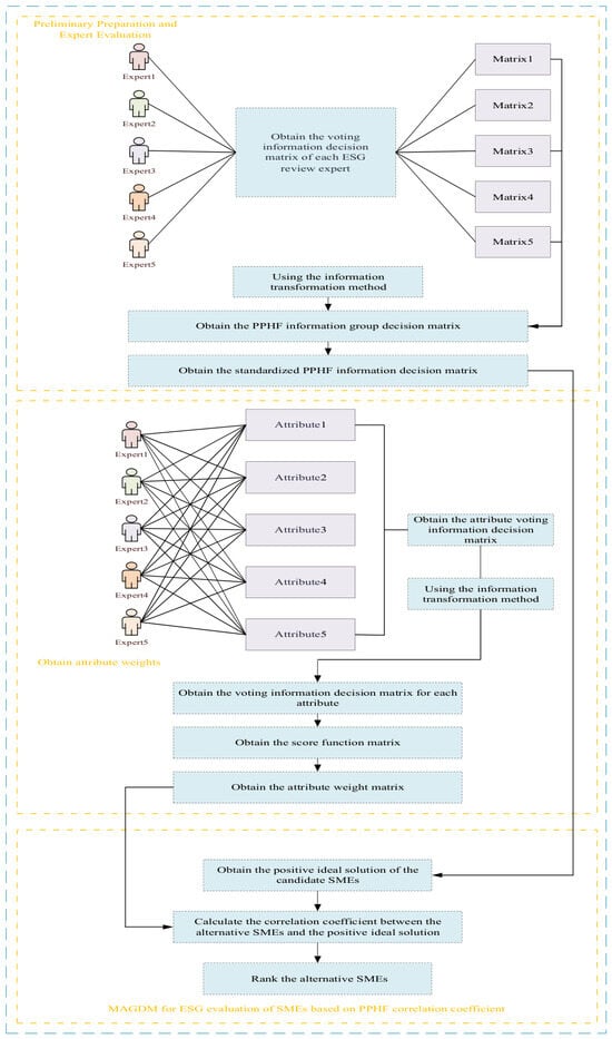
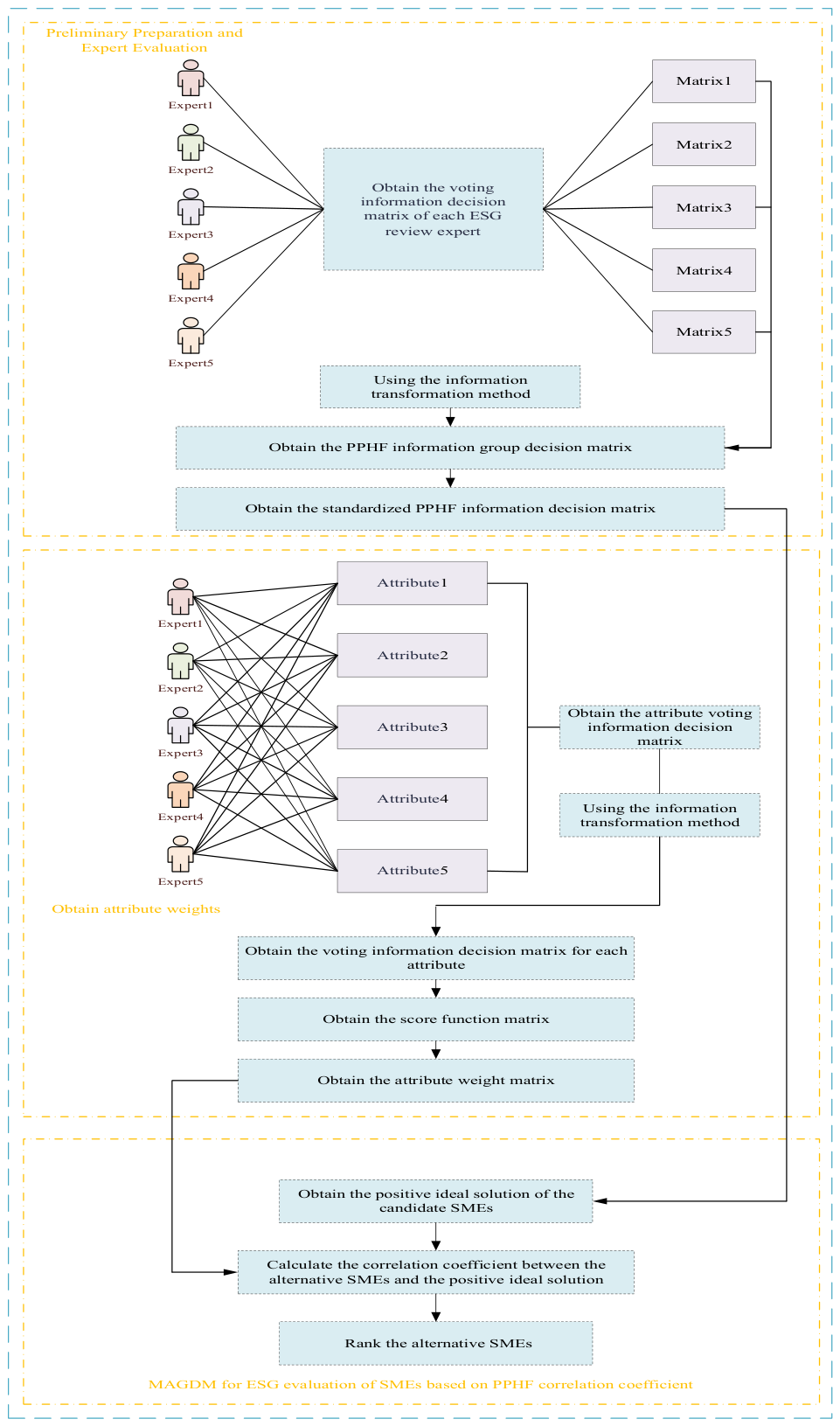
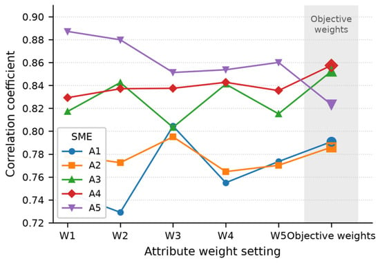
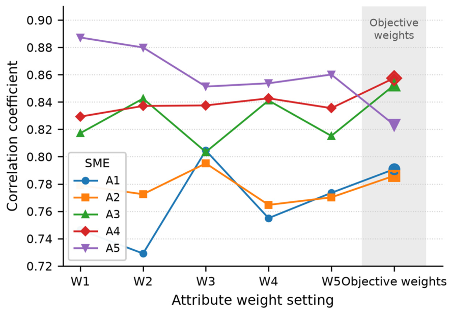

Disclaimer/Publisher’s Note: The statements, opinions and data contained in all publications are solely those of the individual author(s) and contributor(s) and not of MDPI and/or the editor(s). MDPI and/or the editor(s) disclaim responsibility for any injury to people or property resulting from any ideas, methods, instructions or products referred to in the content. |
© 2026 by the authors. Licensee MDPI, Basel, Switzerland. This article is an open access article distributed under the terms and conditions of the Creative Commons Attribution (CC BY) license.