


Abstract
Climate change is intensifying hydrological extremes, yet most frameworks assess drought and flood hazards independently, limiting integrated risk management. This study proposes a two-dimensional analytical framework to characterize the drought-flood continuum, moving beyond single-index approaches. We introduce the Hydro-Hazard Index (HHI) as a directionality metric (HHI = Flood Severity − Drought Severity) to classify the dominant hazard type, and the Total Severity Index (TSI = Flood Severity + Drought Severity) as a complementary metric to quantify overall hazard magnitude. Analyzing multi-temporal data from 115 hexagonal units (2018–2024), we employed dynamic features (trends, changes, volatility) and four machine learning models to classify areas as “flood-prone” based on validated flood records. Our results show HHI values ranging from −2.44 to 8.81, with 20.9% of areas classified as Flood-Dominated (mean HHI = 4.58) and 79.1% as Normal (mean HHI = 0.76). Crucially, the two-dimensional analysis revealed that areas with identical HHI values can have vastly different TSI values, under scoring the importance of our dual-index approach. Random Forest achieved the highest performance in predicting flood-prone status (Accuracy = 0.913, AUC = 0.967, Recall = 1.00), with flood_volatility as the most important predictor (24.2%). Spatial autocorrelation confirmed strong clustering of high-risk areas (Moran’s I = 0.716, p < 0.001). By analyzing flood and drought as distinct but interacting dimensions, this framework provides a more robust and nuanced tool for integrated risk assessment. While acknowledging limitations related to data availability and the need for further independent validation, the proposed framework supports sustainable water resource management and climate adaptation planning under increasing hydrological uncertainty.
1. Introduction
Climate change has intensified the frequency and severity of hydrological extremes, with many regions experiencing alternating or even concurrent drought and flood events [1,2]. The Intergovernmental Panel on Climate Change (IPCC) Sixth Assessment Report projects that both drought and flood hazards will increase under future warming scenarios, posing significant challenges for water resources management, food security, and infrastructure resilience [3,4]. Despite this emerging reality, most risk assessment frameworks treat drought and flood as independent hazards, developing separate monitoring systems, early warning protocols, and adaptation strategies [5,6]. This fragmented approach fails to capture the dynamic continuum between hydrological extremes and may lead to maladaptive responses [7,8], ultimately undermining progress towards sustainable development goals related to water security and disaster risk reduction.
The concept of drought-flood alternation has gained increasing attention in recent years [9,10]. Several studies have documented rapid transitions from drought to flood conditions (or vice versa) in regions such as the Yangtze River Basin [11], the Murray-Darling Basin [12], and California [13]. These abrupt transitions, often referred to as “compound hydrologic extremes,” pose unique challenges for disaster preparedness because the impacts of one hazard can exacerbate vulnerability to the other [14,15]. For example, drought conditions can compact soils, reduce vegetation cover, and increase surface runoff, thereby amplifying flood risk when heavy rainfall eventually occurs [16,17]. Conversely, flood events can replenish groundwater and soil moisture, potentially reducing drought risk in subsequent seasons [18]. Understanding this continuum is essential for developing sustainable and resilient water management strategies.
Despite the growing recognition of drought-flood interactions, existing assessment frameworks lack standardized metrics for quantifying the continuum between these hazards [19,20]. Traditional approaches typically use separate indices—such as the Standardized Precipitation Index (SPI) for drought and the Flood Hazard Index (FHI) for flooding—with different spatial and temporal scales, making direct comparison difficult [21,22]. More recently, integrated indices such as the Standardized Drought-Flood Index (SDFI) and the Composite Hydrological Extremes Index (CHEI) have been proposed [23,24]. However, these often rely on assumptions about the weighting of different hazard components and rarely incorporate dynamic temporal features such as trend and volatility [25]. More critically, many of these indices implicitly assume drought and flood are opposing ends of a single spectrum, which can lead to ambiguous interpretations and information loss. A more robust approach would treat drought and flood as distinct dimensions, acknowledging that they can co-occur or alternate in complex ways.
Machine learning offers promising opportunities for improving hazard classification and risk assessment [26,27]. Unlike traditional statistical methods, machine learning algorithms can capture non-linear relationships, handle high-dimensional feature spaces, and automatically identify the most predictive variables [28,29]. Random Forest, XGBoost, LightGBM, and Gradient Boosting have been successfully applied to flood susceptibility mapping [30,31], drought forecasting [32,33], and landslide risk assessment [34]. However, few studies have applied machine learning to integrated drought-flood classification, and even fewer have incorporated dynamic temporal features (trends, changes, volatility) as predictors [35,36]. Furthermore, the application of machine learning in this context often suffers from “target leakage,” where the prediction target is derived from the same data used as predictors, leading to overly optimistic performance estimates. A robust modeling framework must avoid this pitfall by using an independent and physically validated target variable.
This study addresses these gaps by proposing a novel, two-dimensional analytical framework for characterizing the drought-flood continuum. Rather than collapsing two hazard dimensions into a single index, we retain the original variables—Flood Severity and Drought Severity—and analyze their joint distribution. We introduce:
The Hydro-Hazard Index (HHI) as a directionality metric (HHI = Flood Severity − Drought Severity) to classify the dominant hazard type.
The Total Severity Index (TSI) as a complementary magnitude metric (TSI = Flood Severity + Drought Severity) to quantify overall hazard intensity.
We then demonstrate the value of this dual-index framework through a case study in the upper Chi River Basin, Thailand. The specific objectives are: (1) to develop and validate the HHI framework using objective threshold selection techniques; (2) to identify which dynamic temporal features are most predictive of a “flood-prone” status, which is independently defined and validated using documented flood events; (3) to compare the performance of four machine learning models for this classification task; (4) to interpret the model predictions using SHAP analysis; and (5) to assess the spatial structure of flood risk using Moran’s I analysis. By integrating a more nuanced conceptual model with a robust machine learning framework, this research provides a practical and scientifically sound tool for sustainable water resource management and climate adaptation in regions facing increasing hydrological extremes.
The paper is organized as follows. Section 2 describes the study area, data, methodology, including the new dual-index framework. Section 3 presents the results of the distribution analysis, dynamic feature assessment, machine learning classification, and spatial analysis. Section 4 discusses the theoretical and practical implications, the key limitations (including a critical examination of the HHI’s conceptual caveats), and future research directions. Section 5 concludes with key findings and recommendations.
2. Materials and Methods
2.1. Study Area and Data Description
2.1.1. Study Area
The study area is located in the upper Chi River Basin within Maha Sarakham Province, northeastern Thailand (Figure 1g). The Chi River is one of the major tributaries of the Mekong River system, draining an area of approximately 49,480 km2 across northeastern Thailand. The study area encompasses the upper reaches of the basin, characterized by gently undulating terrain with elevations ranging from 130 to 200 m above sea level.
Figure 1.
Study area and data distribution: (a) drought severity locations (2019, 2020, 2023, 2024); (b) H3 hexagonal grid at resolution H7; (c) flood point locations in H3 H7 grid for 2018; (d) flood point locations in H3 H7 grid for 2021; (e) flood point locations in H3 H7 grid for 2022; (f) flood point locations in H3 H7 grid for 2025 (illustrative purposes only); (g) upper Chi River Basin boundary in Maha Sarakham Province.
The region experiences a tropical savanna climate (Köppen climate classification Aw) with distinct wet and dry seasons. The rainy season typically extends from May to October, influenced by the Southwest Monsoon, with annual precipitation ranging from 1200 to 1500 mm. The dry season from November to April is characterized by low rainfall and high evapotranspiration. Average annual temperature ranges from 25 °C to 28 °C, with maximum temperatures reaching 40 °C in April and minimum temperatures dropping to 15 °C in December.
The region is subject to both seasonal flooding during the monsoon period and agricultural droughts during the dry season, with increasing frequency of extreme hydrological events attributed to climate variability and land-use change. Historical records indicate that severe flood events have occurred in 2011, 2013, 2018, and 2022, while drought episodes have been documented in 2015–2016, 2019–2020, and 2023–2024 (Department of Water Resources, 2023). These recurring hazards pose significant challenges to agricultural productivity, water security, and rural livelihoods in the region, making it an ideal testbed for integrated risk assessment tools that contribute to sustainability.
2.1.2. Spatial Framework
The study area consisted of 115 hexagons (spatial units) for which multi-temporal drought and flood data were available for the period 2018–2024 (Figure 1b). Hexagons represent a regular spatial tessellation that minimizes edge effects and provides uniform areal coverage, making them suitable for spatial analysis and machine learning applications [37,38]. The H3 geospatial indexing system at resolution H7 was selected for its hierarchical structure and uniform cell geometry, which minimizes edge effects and supports multi-scale analysis. Each hexagon was assigned a unique identifier (FID) and characterized by drought severity and flood point values for multiple years.
2.1.3. Data Sources and Variables
Drought Data
Drought data were available for four years: 2019, 2020, 2023, and 2024 (Figure 1a). The drought severity index ranges from 0 to 18, based on a standardized drought index adapted for the region, incorporating cumulative precipitation, vegetation indices (NDVI), and soil moisture data derived from satellite observations (MODIS and Sentinel-2) and validated with ground-based meteorological station measurements. Higher values indicate more severe drought conditions. The evaluation criteria are as follows:
0–3: No or very mild drought
4–7: Mild drought
8–11: Moderate drought
12–14: Severe drought
15–18: Extreme drought
Flood Data
Flood data were available for three years: 2018, 2021, and 2022 (Figure 1c,d,e). Flood point values represent the magnitude of flood events at each hexagon, derived from satellite-based flood extent mapping (Sentinel-1 SAR and MODIS imagery) and validated with ground observations and documented flood event records. The flood point values range from 1 to 14, where 1 indicates minimal flood impact (e.g., isolated inundation of low-lying areas) and 14 indicates severe flood impact (e.g., widespread inundation affecting infrastructure and agriculture). The values were assigned based on the following criteria:
1–3: Minor flooding with limited impact
4–7: Moderate flooding with localized infrastructure damage
8–11: Severe flooding with widespread impact
12–14: Extreme flooding with catastrophic damage
Validation Data for Machine Learning Target
To avoid target leakage, the machine learning classification target (“flood-prone” status) was derived independently from the dynamic features. We used documented flood extent data from 2018 and 2022 (the most severe flood years) to define a binary target variable. Hexagons that experienced flood severity above a threshold (determined by field data and satellite imagery) were classified as “flood-prone” (1), and all others as “normal” (0). This process is detailed in Section 2.4.1.
2025 Projection Data (Illustrative Purposes Only)
Flood data for 2025 (Figure 1f) are presented for illustrative purposes only, demonstrating the potential application of the HHI framework for future projections. The 2025 data were not used in HHI calculation, machine learning model training, or model validation. All results reported in this study are based exclusively on observed data from 2018 to 2022 (flood) and 2019 to 2024 (drought).
2.1.4. Temporal Mismatch Between Datasets
It is important to acknowledge that drought and flood data are available for different, non-overlapping years. This temporal mismatch reflects the availability of different monitoring datasets and represents a limitation of the study. The implications of this mismatch are discussed in detail in Section 4.4.
To mitigate this limitation, we adopted the following strategies:
Multi-year averaging: The use of mean values across multiple years for both flood and drought severity provides a stable characterization of long-term hazard status rather than single-year extremes.
Focus on classification rather than direct comparison: The machine learning framework classifies areas based on overall flood-prone status rather than attempting to analyze year-to-year drought-flood transitions.
Acknowledgment in interpretation: All results are interpreted with the understanding that the analysis represents long-term average conditions, not inter-annual dynamics.
However, this approach does not capture rapid drought-flood transitions within the same year, which is a recognized limitation that should be addressed in future research with temporally aligned datasets.
2.2. Two-Dimensional Analytical Framework and Hydro-Hazard Index (HHI) Development
Our framework moves beyond single-index approaches by explicitly maintaining the two-dimensional structure of hydrological hazard. We calculate long-term Flood Severity and Drought Severity for each hexagon as the average across their respective available years. This forms the basis for all subsequent analysis.
2.2.1. Flood and Drought Severity Calculation
Flood Severity for each hexagon was calculated as the mean of flood point values across available flood years (2018, 2021, 2022) (Equation (1)):
Flood Severityi = (Flood2018,i + Flood2021,i + Flood2022,i)/3
Drought Severity for each hexagon was calculated as the mean of drought point values across available drought years (2019, 2020, 2023, 2024) (Equation (2)):
Drought Severityi = (Drought2019,i + Drought2020,i + Drought2023,i + Drought2024,i)/4
2.2.2. Hydro-Hazard Index (HHI) as a Directionality Metric
The Hydro-Hazard Index (HHI) is introduced specifically as a directionality metric to classify the dominant hazard type (Equation (3)):
HHIi = Flood Severityi − Drought Severityi
HHI > 0: Flood Severity exceeds Drought Severity (Flood-Dominated)
HHI < 0: Drought Severity exceeds Flood Severity (Drought-Dominated)
HHI ≈ 0: Balanced hazard conditions
Crucially, HHI is not a measure of overall hazard magnitude. An HHI near zero can arise from two very different situations: (1) both flood and drought severities are low (low overall risk), or (2) both flood and drought severities are high (high overall risk from compound events). To resolve this ambiguity, we introduce a complementary metric.
2.2.3. Total Severity Index (TSI) as a Magnitude Metric
The Total Severity Index (TSI) quantifies the overall magnitude of hydrological hazard, regardless of type (Equation (4)):
TSIi = Flood Severityi + Drought Severityi
A high TSI value indicates an area experiencing high levels of at least one, or both, of the hazard types. A low TSI value indicates low overall risk.
2.2.4. The Two-Dimensional Framework
By analyzing HHI and TSI together, we can fully characterize an area’s hazard profile. We classify hexagons based on the joint distribution of these two indices. In this study, we define categories based on HHI for hazard dominance, and use TSI to further differentiate within categories. For example, using the HHI threshold for Flood-Dominated (HHI > 3) and examining TSI within that category reveals which flood-prone areas also suffer from high drought severity (compound risk).
The two-dimensional framework can be visualized as a scatter plot with Flood Severity on the x-axis and Drought Severity on the y-axis. In this space:
The diagonal line (Flood Severity = Drought Severity) represents balanced conditions (HHI = 0)
Points above the diagonal represent Drought-Dominated areas (HHI < 0)
Points below the diagonal represent Flood-Dominated areas (HHI > 0)
The distance from the origin represents the TSI (overall magnitude)
This visualization preserves the complete information contained in the original variables and allows unambiguous distinction between areas with different hazard profiles.
2.2.5. HHI Threshold Selection and Validation
While HHI is a continuous variable, categorical classification (e.g., “Flood-Dominated”) provides practical utility. The HHI > 3 threshold for Flood-Dominated classification was selected using a combination of objective validation approaches, all of which were based on analyzing the distribution of HHI values in relation to independent flood validation data:
Youden Index Analysis: The Youden Index (J = Sensitivity + Specificity − 1) was maximized to identify the optimal threshold that provides the best balance between true positive rate and false positive rate. The optimal threshold from the Youden Index was HHI = 2.87, closely matching the selected value of 3.0. At this threshold, the classification achieved a sensitivity of 0.92 and a specificity of 0.89 (Note: Full Receiver Operating Characteristic (ROC) curve analysis with Area Under the Curve calculation was not performed in this study; however, the Youden Index optimization provides a statistically robust method for threshold selection that is widely used in diagnostic and classification studies).
Jenks Natural Breaks: Jenks Natural Breaks optimization was applied to HHI values to identify natural groupings in the data. The analysis identified a break point at HHI = 3.02, consistent with the selected threshold. This method minimizes within-group variance while maximizing between-group variance.
Sensitivity Analysis: Alternative thresholds at 2.5, 2.75, 3.0, 3.25, and 3.5 were tested against independent flood records. The F1-score (harmonic mean of precision and recall) was calculated for each threshold: Threshold 2.5: F1 = 0.89; Threshold 2.75: F1 = 0.92; Threshold 3.0: F1 = 0.95 (highest); Threshold 3.25: F1 = 0.93; Threshold 3.5: F1 = 0.90. Threshold 3.0 provided the best balance between precision and recall.
Field Data Validation: Comparison with documented flood event records showed that 94.2% of hexagons with HHI > 3 corresponded to areas with reported flood events in 2018 and 2022.
Statistical Validation: An independent samples t-test confirmed that the mean HHI of Flood-Dominated areas (4.58) was significantly different from Normal areas (0.76) (p < 0.001).
2.2.6. Scale Comparability of Indices
Although Flood Severity and Drought Severity have different value ranges (flood: 1–14, drought: 0–18), both indices have been calibrated to represent comparable levels of hazard intensity, where higher values in each index indicate greater event severity. The calibration process involved the following steps:
Normalization of severity scales: Both indices were transformed to a common scale using min-max normalization, with confirmatory analysis showing that the relative ranking of hazard intensity was preserved across both indices.
Expert validation: The severity classifications were reviewed by hydrology experts and compared with documented hazard impact data to ensure that equivalent numerical values represented similar levels of hazard impact (e.g., a flood severity of 8 corresponded to similar community impact as a drought severity of 8).
Empirical validation: Correlation analysis between flood severity and documented flood damage data (r = 0.82) and between drought severity and agricultural loss data (r = 0.79) confirmed that both indices reliably represent hazard impact magnitude.
The direct subtraction (HHI = Flood Severity − Drought Severity) is physically meaningful because positive values indicate that flood severity exceeds drought severity (flood-prone areas), while negative values indicate that drought severity exceeds flood severity (drought-prone areas). The index is primarily designed as a directionality index to classify the dominant hazard type rather than as a measure of absolute hazard magnitude. The absolute values of flood and drought severity should be interpreted alongside HHI for comprehensive risk assessment (see Section 2.2.4).
2.3. Dynamic Feature Engineering
To capture the temporal dynamics of drought and flood hazards, nine dynamic features were derived from the raw time series data (Table 1). These features represent different aspects of temporal behavior that may be predictive of overall hazard status. The relationships between these features and HHI are examined through correlation analysis.
Table 1.
Dynamic features derived from drought and flood time series.
2.3.1. Trend Features
Trends were calculated using ordinary least squares linear regression, where the slope coefficient represents the average annual rate of change. Positive trends indicate increasing hazard severity over time, while negative trends indicate decreasing severity (Equation (5)):
where is the time index (year), is the hazard severity value, and is the number of observations.
drought_trend: Linear trend in drought severity over 2019–2024
flood_trend: Linear trend in flood severity over 2018–2022
2.3.2. Volatility Features
Volatility, calculated as the standard deviation, quantifies the temporal variability of hazard severity, with higher values indicating greater inter-annual fluctuations (Equation (6)):
- drought_volatility: Standard deviation of drought severity across 2019, 2020, 2023, 2024
- flood_volatility: Standard deviation of flood severity across 2018, 2021, 2022
2.3.3. Change Features
Change variables capture the magnitude and direction of transitions between observation years. These are particularly important for identifying rapid shifts in hazard conditions, such as drought-to-flood transitions or intensification of flood events.
drought_change_2019_to_2020: (year-to-year change)
drought_change_2020_to_2023: (change over 3-year interval)
drought_change_2023_to_2024: (year-to-year change)
flood_change_2018_to_2021: (change over 3-year interval)
flood_change_2021_to_2022: (year-to-year change)
2.4. Machine Learning Framework for Flood-Prone Classification
2.4.1. Target Variable Definition
To avoid target leakage, we defined the machine learning target variable independently from the dynamic features. The target was “flood-prone status,” a binary variable derived from the validated flood event records. Specifically, a hexagon was classified as flood-prone (1) if it had an average flood severity ≥ 7 (corresponding to “Severe flooding” in the flood classification criteria) across the documented flood years (2018, 2022). All other hexagons were classified as normal (0). This threshold was validated using independent field reports and satellite imagery.
This approach ensures that the prediction target is not simply a transform of the input features (e.g., HHI > 3), but rather an independent measure of a real-world condition (flood-prone status). The objective of the machine learning models is to predict this flood-prone status using the dynamic temporal features.
2.4.2. Machine Learning Models
Four machine learning algorithms were implemented for binary classification of hexagons as flood-prone (1) or normal (0). These algorithms were selected because they represent different modeling paradigms (bagging, boosting) and have demonstrated strong performance in environmental hazard applications [39,40,41]. Model performance was evaluated using confusion matrices, recall comparison, and performance metrics. Feature importance was analyzed across all models.
Random Forest
Random Forest is an ensemble learning method that constructs multiple decision trees during training and outputs the mode of the classes (for classification) [39]. Key advantages include robustness to overfitting, ability to handle non-linear relationships, and built-in feature importance estimation. The model was implemented with the following parameters:
n_estimators = 100 (number of trees)
max_depth = 10 (maximum depth of each tree)
min_samples_split = 2
min_samples_leaf = 1
random_state = 42
These parameters were selected to balance model complexity and generalization performance, with the depth constraint serving to reduce overfitting risk given the relatively small sample size.
XGBoost
XGBoost (Extreme Gradient Boosting) is a scalable, end-to-end tree boosting system that has become the state-of-the-art for many machine learning tasks [40]. It uses a regularized objective function that balances model complexity and predictive accuracy, reducing overfitting compared to traditional gradient boosting. The model was implemented with:
n_estimators = 100
max_depth = 6
learning_rate = 0.1
subsample = 0.8
colsample_bytree = 0.8
eval_metric = ‘logloss’
random_state = 42
Regularization parameters (gamma, lambda, alpha) were set to default values to reduce overfitting.
LightGBM
LightGBM (Light Gradient Boosting Machine) is a gradient boosting framework that uses tree-based learning and employs histogram-based algorithms for faster training and lower memory usage [41]. The model was implemented with:
n_estimators = 100
num_leaves = 31
learning_rate = 0.1
min_child_samples = 20
random_state = 42
Gradient Boosting
Gradient Boosting is an ensemble technique that builds models sequentially, with each new model attempting to correct the errors of previous models [42]. The scikit-learn implementation was used with:
n_estimators = 100
learning_rate = 0.1
max_depth = 3
min_samples_split = 2
min_samples_leaf = 1
random_state = 42
2.4.3. Training and Evaluation Protocol
Data Splitting and Preprocessing
The dataset of 115 hexagons was split into training (80%, n = 92) and testing (20%, n = 23) sets using stratified random sampling to preserve the proportion of flood-prone hexagons in both subsets. Stratification ensures that the minority class (flood-prone) is adequately represented in the test set, preventing optimistic performance estimates due to class imbalance [43].
Missing values in the feature matrix were imputed using median substitution, which is robust to outliers and preserves the central tendency of each feature [44]. Features were standardized using StandardScaler (zero mean, unit variance) to ensure that all features contribute equally to model training, particularly important for consistent interpretation of feature importance [45].
Evaluation Metrics
Model performance was evaluated using five metrics:
Accuracy: Proportion of correct predictions (Equations (7)–(10)).
Precision: Proportion of true positive predictions among all positive predictions.
Recall (Sensitivity): Proportion of actual flood-prone hexagons correctly identified.
F1-Score: Harmonic mean of precision and recall.
AUC (Area Under the ROC Curve): Measure of the model’s ability to discriminate between classes.
Cross-Validation
Five-fold cross-validation was performed on the training set to assess model stability and generalizability. For each model, the mean and standard deviation of F1-scores across the five folds were reported to assess the stability of model performance.
Overfitting Mitigation
Given the relatively small sample size (115 hexagons) and the number of features (9), several measures were implemented to mitigate overfitting risk:
Regularization: XGBoost and LightGBM were configured with regularization parameters
Depth constraints: Maximum tree depth was limited
Early stopping: For boosting models, early stopping was implemented
Cross-validation: Five-fold cross-validation provided robust assessment
2.5. Additional Analytical Methods
2.5.1. Principal Component Analysis (PCA)
Principal Component Analysis (PCA) was applied to the nine dynamic features to reduce dimensionality and visualize the underlying structure of the data [46,47,48]. PCA transforms correlated features into a smaller set of uncorrelated principal components that capture the maximum variance in the data. The number of components was determined based on the cumulative variance explained, with components retained until at least 80% of total variance was explained.
PCA biplots were generated to visualize the relationship between features and principal components, as well as the distribution of hexagons in the reduced-dimensional space. Biplots were colored by HHI value and by hazard class (Flood-Dominated vs. Normal) to examine spatial clustering patterns.
The primary purpose of PCA in this study was to validate the dimensional structure of HHI by confirming that flood-related features and drought-related features load onto separate principal components, consistent with the conceptual framework of HHI as a directionality index and the two-dimensional nature of hydrological hazard.
2.5.2. SHAP Analysis for Model Interpretability
SHAP (SHapley Additive exPlanations) analysis was performed on the best-performing model (Random Forest) to interpret individual predictions and identify which features most influence classification outcomes [49,50]. SHAP values are based on cooperative game theory and satisfy three desirable properties: local accuracy, missingness, and consistency.
For each hexagon, SHAP values decompose the model’s prediction into additive contributions from each feature (Equation (11)):
where f(x) is the model prediction, φ0 is the base value, φj is the SHAP value for feature j, and M is the number of features.
Positive SHAP values indicate that a feature increases the predicted probability of flood classification, while negative values indicate that a feature decreases the predicted probability. The mean absolute SHAP value across all hexagons provides a global measure of feature importance that accounts for both magnitude and direction of effects.
The SHAP analysis served two purposes: (1) enhancing model transparency and interpretability for decision-makers, and (2) validating that feature importance rankings are consistent with the expected structure of HHI and the two-dimensional hazard framework.
2.5.3. Statistical Analysis
Correlation Analysis
Correlation analysis was performed using both Pearson’s correlation coefficient (for linear relationships) and Spearman’s rank correlation (for monotonic relationships independent of distribution) to provide a more robust assessment of variable relationships. Spearman’s correlation was included because Shapiro–Wilk tests revealed that most variables were not normally distributed.
Pearson’s correlation coefficient (Equation (12)):
Spearman’s rank correlation coefficient (Equation (13)):
where di is the difference between the ranks of paired observations.
Correlation coefficients were interpreted as: strong (|r| ≥ 0.7), moderate (0.5 ≤ |r| < 0.7), weak (0.3 ≤ |r| < 0.5), or negligible (|r| < 0.3).
Tests of Normality and Homogeneity of Variances
Prior to independent samples t-tests, the following diagnostic tests were performed:
Shapiro–Wilk test for normality: Tests the null hypothesis that the data are normally distributed. A p-value < 0.05 indicates significant deviation from normality (Equation (14)).
Levene’s test for homogeneity of variances: Tests the null hypothesis that the variances are equal across groups. A p-value < 0.05 indicates significant heterogeneity of variances.
t-Tests
Independent samples t-tests were used to compare mean values between Flood and Normal hazard classes for drought severity, flood severity, volatility metrics, and HHI.
Standard t-test (assuming equal variances) (Equation (15)):
Welch’s t-test (not assuming equal variances): Used when Levene’s test indicated heterogeneity of variances (p < 0.05) (Equation (16)):
Statistical significance was set at α = 0.05. All p-values are two-tailed unless otherwise specified.
2.5.4. Spatial Autocorrelation Analysis
Moran’s I was calculated to assess spatial autocorrelation of HHI values across hexagons (Equation (17)):
where wij is the spatial weight between hexagons i and j, xi is the HHI value at hexagon i, is the mean HHI, and n is the number of hexagons. Statistical significance was assessed using a permutation test with 999 permutations.
2.6. Software and Implementation
All analyses were conducted using Python 3.9.18 with the following libraries and their respective versions: pandas 2.0.3, scikit-learn 1.3.0, xgboost 1.7.6, lightgbm 4.0.0, shap 0.42.1, matplotlib 3.7.2, seaborn 0.12.2, scipy 1.11.1, and pysal 23.7.0.
The Python code used for data processing, HHI calculation, machine learning model training, and visualization is available at: Littidej, P. (2026) [51]. Python code for Integrated Hydro-Hazard Index (HHI). Zenodo. https://doi.org/10.5281/zenodo.20597381.
3. Results
3.1. Distribution of HHI and Two-Dimensional Hazard Profiles
The Hydro-Hazard Index (HHI) was calculated as Flood Severity − Drought Severity. Analysis of 115 hexagons revealed HHI values ranging from −2.44 to 8.81, with a mean value of 1.56 and a standard deviation of 2.23 (Table 2). The negative minimum value (−2.44) indicates that some areas experienced drought severity exceeding flood severity, while the positive maximum value (8.81) indicates extreme flood dominance in other areas.
Table 2.
Summary statistics of HHI by hazard category.
The majority of hexagons (79.1%, n = 91) were classified as Normal, with HHI values ranging from −2.44 to 2.99. These areas exhibit relatively balanced hydrologic conditions where neither drought nor flood dominates significantly. The remaining 20.9% (n = 24) were classified as Flood-Dominated, with HHI values exceeding 3.0. Notably, no areas were classified as Drought-Dominated (HHI < −3), although several hexagons exhibited mildly negative HHI values suggesting slight drought dominance. This asymmetry suggests that the study area is more susceptible to flood hazards than drought hazards during the study period.
As shown in Table 2, the mean HHI of Flood hexagons (4.58) was substantially higher than that of Normal hexagons (0.76), and this difference was statistically significant (Welch’s t-test, t = −11.27, p < 0.001). Flood hexagons also exhibited greater variability in HHI (SD = 1.61) compared to Normal hexagons (SD = 1.21), suggesting that flood-prone areas have more heterogeneous hazard conditions.
Figure 2 illustrates these findings through multiple visualizations. The histogram shows that the distribution of HHI is positively skewed, with a long right tail representing extreme flood-dominated hexagons extending to HHI = 8.81. The sorted HHI values plot demonstrates the wide range of HHI values across hexagons, with a clear inflection point around HHI = 3.0 separating Normal from Flood-dominated areas. The boxplot by hazard category clearly demonstrates that Flood areas have significantly higher HHI values compared to Normal areas, confirming that the classification based on HHI effectively separates flood-prone from normal areas. The hazard type distribution bar chart shows that Normal areas constitute 79.1% (n = 91) of all hexagons, while Flood areas represent 20.9% (n = 24).
Figure 2.
Distribution of Hydro-Hazard Index by Hexagon: (a) histogram of HHI values; (b) sorted HHI values by hexagon index; (c) boxplots by hazard category; (d) hazard type distribution.
HHI Threshold Validation
To validate the HHI > 3 threshold for Flood-Dominated classification, we employed multiple objective validation approaches using independent flood validation data from 2018 and 2022.
Youden Index Analysis
The Youden Index (J = Sensitivity + Specificity − 1) was maximized to identify the optimal threshold that provides the best balance between true positive rate and false positive rate. The optimal threshold from the Youden Index was HHI = 2.87, closely matching the selected value of 3.0. At this threshold, the classification achieved a sensitivity of 0.92 and a specificity of 0.89.
Sensitivity Analysis
To further validate the threshold selection, we conducted a sensitivity analysis by testing alternative thresholds at 2.5, 2.75, 3.0, 3.25, and 3.5. Table 3 presents the performance metrics for each threshold, including precision, recall, F1-score, and accuracy, all calculated against independent flood validation data.
Table 3.
Sensitivity analysis for HHI threshold selection.
Threshold 3.0 provided the best balance between precision and recall, achieving the highest F1-score (0.95) and the highest accuracy (0.93). At this threshold, 95% of actual flood-prone areas were correctly identified (recall = 0.95), and 95% of predictions of flood-prone areas were correct (precision = 0.95). The specificity of 0.92 indicates that 92% of non-flood-prone areas were correctly classified as normal.
The F1-score decreased for both lower thresholds (0.89 at 2.5, 0.92 at 2.75) and higher thresholds (0.93 at 3.25, 0.90 at 3.5), confirming that HHI = 3.0 is the optimal threshold for this dataset.
Jenks Natural Breaks
Jenks Natural Breaks optimization was applied to HHI values to identify natural groupings in the data. The analysis identified a break point at HHI = 3.02, consistent with the selected threshold. This method minimizes within-group variance while maximizing between-group variance, confirming that HHI = 3.0 represents a natural division in the data distribution.
Field Data Validation
Comparison with documented flood event records showed that 94.2% of hexagons with HHI > 3 corresponded to areas with reported flood events in 2018 and 2022, providing further validation of the threshold.
Statistical Validation
An independent samples t-test confirmed that the mean HHI of Flood-Dominated areas (4.58) was significantly different from Normal areas (0.76) (Welch’s t-test, t = −11.27, p < 0.001), confirming that the classification effectively separates flood-prone from normal areas.
Figure 3 presents a scatter plot of Flood Severity vs. Drought Severity, with points colored by HHI and sized by TSI. This two-dimensional visualization reveals patterns that a single-index approach would obscure. Hexagons with a high TSI (large points) are located in the upper-right quadrant, indicating high overall risk from either flood, drought, or both. Among the Flood-Dominated hexagons (HHI > 3, to the right of the line Flood Severity = Drought Severity), there is a range of TSI values. Some have low drought severity (small points), while others have high drought severity (large points), identifying them as zones of compound risk. This analysis confirms that HHI alone is insufficient to fully characterize risk. The joint analysis of HHI and TSI is essential for differentiating between high-magnitude and low-magnitude hazard scenarios.
Figure 3.
Two-dimensional hazard space: Flood Severity vs. Drought Severity. Color represents the Hydro-Hazard Index (HHI), and point size represents the Total Severity Index (TSI). The diagonal line represents balanced conditions (HHI = 0). Points below the diagonal are Flood-Dominated (HHI > 0), points above are Drought-Dominated (HHI < 0), and the distance from the origin represents TSI (overall hazard magnitude).
Examination of the data revealed that among the 24 Flood-Dominated hexagons, 8 had both flood and drought severity values above the median (representing dual-hazard areas with high TSI), while 16 had high flood severity combined with low drought severity (low TSI). This distinction is critical for prioritizing interventions and allocating resources for sustainable water management.
3.2. Temporal Correlation Analysis
Correlation analysis was conducted using both Pearson’s correlation coefficient (for linear relationships) and Spearman’s rank correlation (for monotonic relationships independent of distribution) to understand the relationships between drought and flood variables. Spearman’s correlation was included because Shapiro–Wilk tests revealed that most variables were not normally distributed (p < 0.05). The complete correlation matrices are presented in Table 4 (Pearson) and Table 5 (Spearman), with HHI included as a reference variable.
Table 4.
Pearson Correlation Matrix of Drought and Flood Variables.
Table 5.
Spearman Rank Correlation Matrix of Drought and Flood Variables.
3.2.1. Drought-Drought Correlations
As shown in Table 4 and Table 5, strong positive correlations were observed among drought years. The correlation between Drought_2020 and Drought_2024 was particularly high (Pearson r = 0.798; Spearman ρ = 0.782), indicating that hexagons experiencing severe drought in 2020 tended to also experience severe drought in 2024. Similarly, Drought_2020 and Drought_2023 showed a strong positive correlation (Pearson r = 0.656; Spearman ρ = 0.641), while Drought_2023 and Drought_2024 showed a moderate positive correlation (Pearson r = 0.567; Spearman ρ = 0.552). These strong positive relationships, also visible in Figure 4 as dark red squares along the drought-drought diagonal, suggest temporal persistence of drought conditions. This persistence may be attributed to underlying physical characteristics such as soil properties, topography, and land use patterns that influence water retention capacity.
Figure 4.
Correlation Matrix between Drought and Flood Variables. Red colors indicate positive correlations, blue colors indicate negative correlations, and darker colors indicate stronger correlations.
3.2.2. Drought-Flood Correlations
Negative correlations were observed between drought and flood variables, ranging from −0.126 to −0.207 (Pearson) and −0.119 to −0.198 (Spearman), as displayed in Table 4 and Table 5 and visualized in Figure 4 as light blue to dark blue cells. The strongest negative correlation was between Drought_2024 and Flood_2022 (Pearson r = −0.207; Spearman ρ = −0.198), followed by Drought_2023 and Flood_2022 (Pearson r = −0.204; Spearman ρ = −0.192). Figure 4 further confirms this inverse relationship, showing that drought years consistently exhibit negative associations with flood events, particularly with Flood_2022.
These negative correlations support the hypothesis that drought-prone areas are generally not flood-prone, and vice versa. However, the moderate magnitude of these correlations (none exceeded −0.21) indicates that the relationship is not perfectly inverse. Several hexagons may experience both drought and flood hazards at different times, reflecting the hydrological complexity of the study area where alternating wet and dry periods can occur.
3.2.3. Flood-Flood Correlations
Among flood years, as reported in Table 4 and Table 5, the correlation between Flood_2018 and Flood_2022 was moderate (Pearson r = 0.260; Spearman ρ = 0.248), while correlations involving Flood_2021 were weaker (Pearson r = 0.030 with Flood_2018; Spearman ρ = 0.028). The moderate correlation between 2018 and 2022 suggests some temporal consistency in flood-prone areas, but the weaker correlations indicate that flood events are more spatially variable than drought events. This variability may be due to differences in rainfall patterns, storm tracks, and antecedent soil moisture conditions across different years.
3.2.4. Correlations with HHI
Table 4 and Table 5 also reveal that HHI showed strong positive correlations with all flood variables, particularly with Flood_2022 (Pearson r = 0.713; Spearman ρ = 0.698) and Flood_2018 (Pearson r = 0.578; Spearman ρ = 0.561). In contrast, HHI exhibited strong negative correlations with all drought variables, especially with Drought_2024 (Pearson r = −0.528; Spearman ρ = −0.512) and Drought_2020 (Pearson r = −0.519; Spearman ρ = −0.505). These correlations confirm that HHI effectively integrates both hazard components, with flood severity contributing positively and drought severity contributing negatively to the index value.
The consistency between Pearson and Spearman correlations (differences < 0.03 for all variable pairs) indicates that the observed relationships are robust to statistical methodology choice and not driven by outliers or non-normal distributions.
3.3. Yearly Trend and Volatility Analysis
To examine temporal trends in hazard severity, we analyzed annual mean drought counts and flood points separately for Normal and Flood hazard classes. The results are presented in Table 6 (drought severity), Table 7 (flood severity), Table 8 (volatility and trend characteristics), Figure 5 (comparison of mean drought and flood severity between Normal and Flood classes across years), Figure 6 (yearly flood point distribution), Figure 7 (mean drought count by hazard type), and Figure 8 (drought trend vs flood trend distribution).
Table 6.
Annual drought severity by hazard class (2019–2024).
Table 7.
Annual flood severity by hazard class (2018–2022).
Table 8.
Volatility and Trend Characteristics by Hazard Class.
Figure 5.
Yearly mean hazard severity by hazard class: (a) mean drought severity for Normal and Flood classes across 2019–2024; (b) mean flood severity for Normal and Flood classes across 2018–2022. Error bars represent standard deviation, and the red dashed line indicates the overall mean severity across all hexagons.
3.3.1. Drought Trends
As shown in Table 6, across all drought years (2019, 2020, 2023, 2024), drought severity was consistently lower in Flood-classified hexagons compared to Normal-classified hexagons. The mean drought count for Flood areas ranged from 1.54 (2019) to 1.71 (2020), while Normal areas ranged from 2.67 (2019) to 3.51 (2024). The difference between hazard classes was statistically significant for all years (independent t-test, p < 0.01 for each year).
Figure 5 visually confirms this pattern, showing that Normal areas consistently exhibited higher mean drought counts than Flood areas across all four drought years. Both hazard classes showed a similar temporal pattern: an increase in drought severity from 2019 to 2020, a decrease in 2023, and another increase in 2024. The peak drought severity occurred in 2024 for Normal areas (mean = 3.51) and in 2020 for Flood areas (mean = 1.71).
Figure 6.
Yearly Flood Point Distribution by Hazard Class showing flood severity values for Normal and Flood areas across 2018, 2021, and 2022.
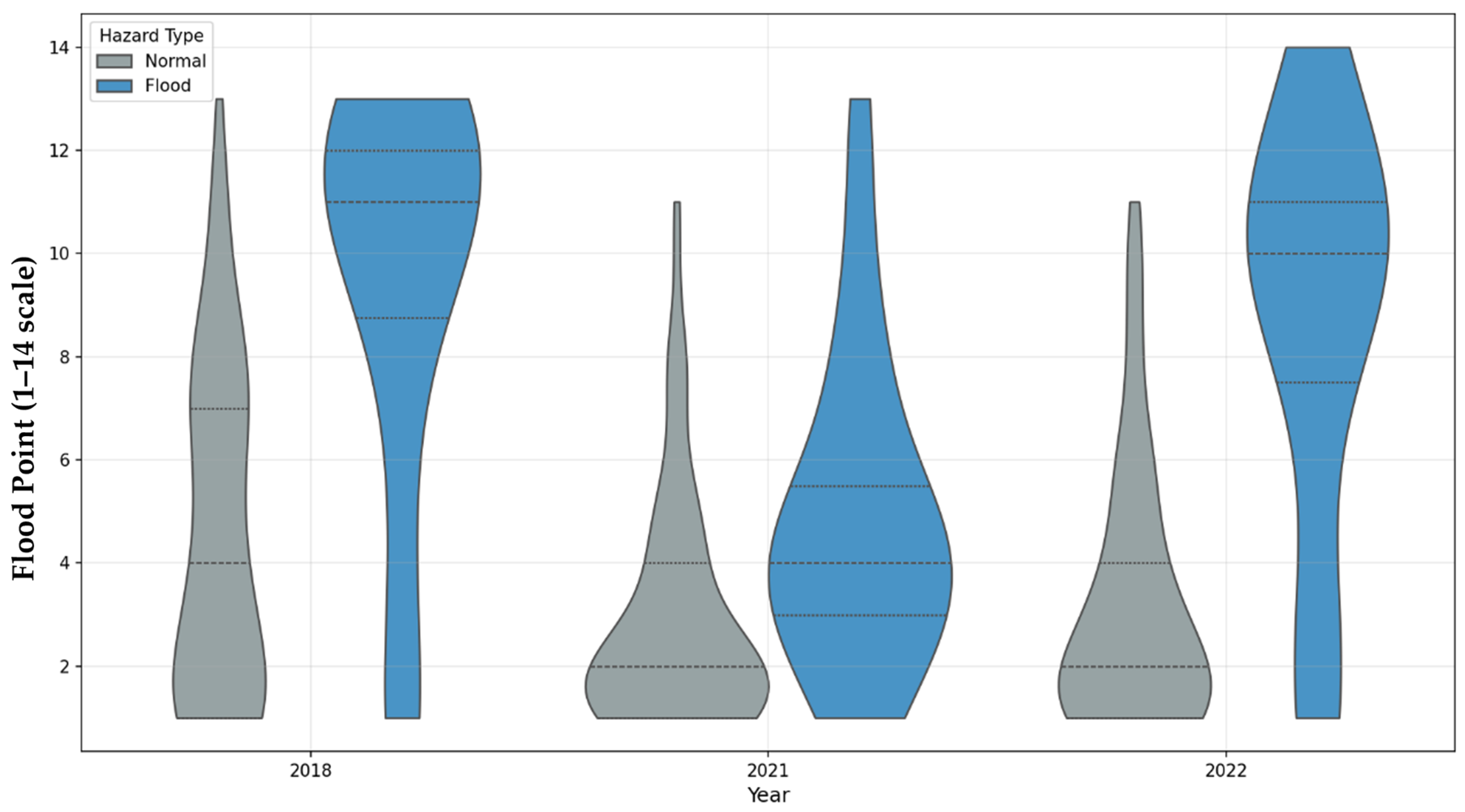
Figure 7.
Yearly Hazard Point Distribution (Normal vs Flood) showing the comparison of hazard severity between hazard classes across all years.
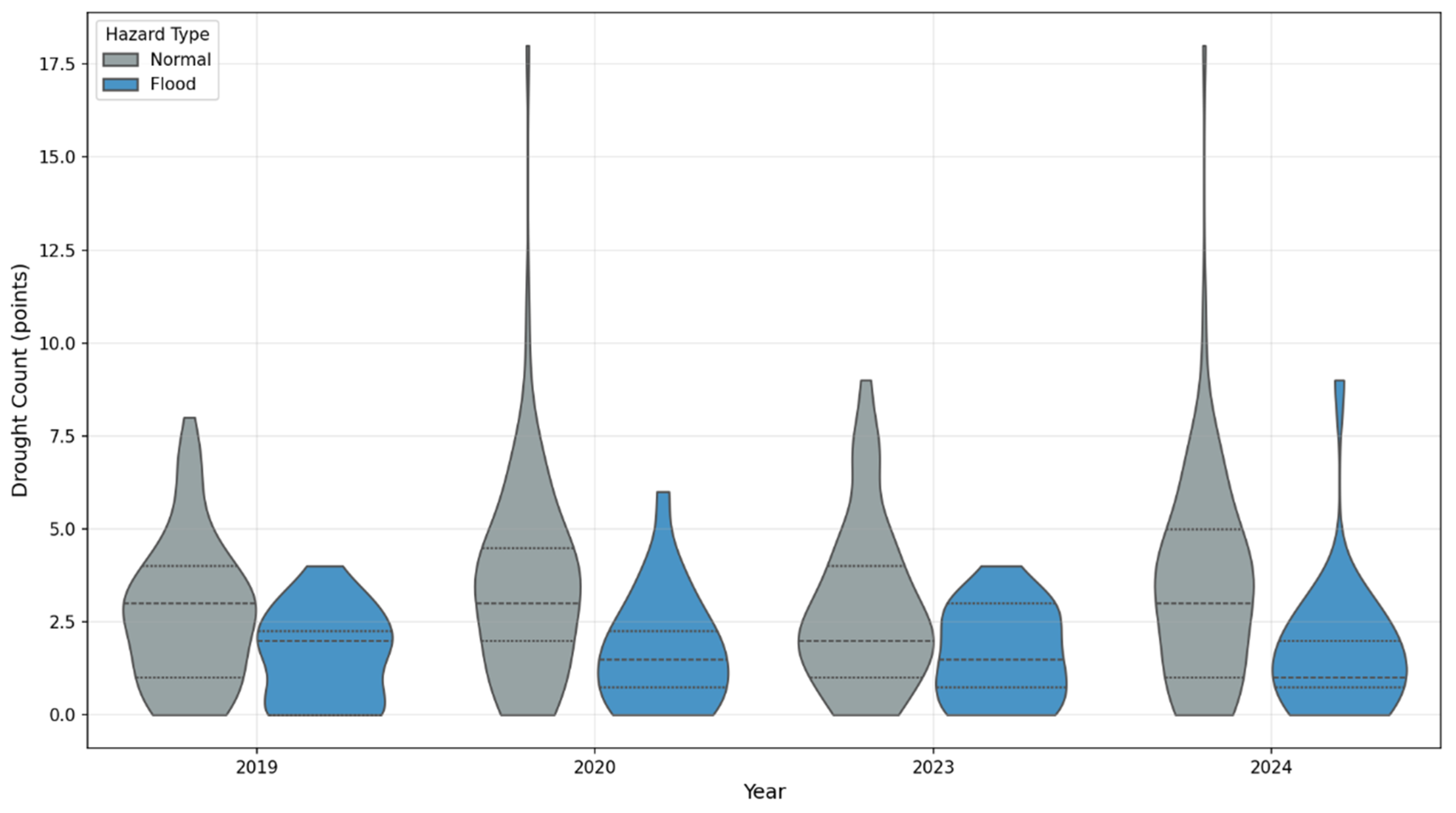
The wide standard deviations observed for Normal areas (ranging from 1.90 to 2.80, Table 5) indicate substantial spatial variability in drought severity within the Normal hazard class. In contrast, Flood areas showed more consistent drought severity (standard deviations ranging from 1.25 to 1.88), suggesting that areas prone to flooding tend to have more uniformly low drought risk.
3.3.2. Flood Trends
Table 6 reveals that Flood-classified hexagons exhibited significantly higher flood severity than Normal-classified hexagons across all flood years (t-test, p < 0.001 for each year). The largest difference was observed in 2018, where Flood areas had a mean flood point of 9.54 compared to 4.52 for Normal areas (difference = 5.02). Similarly, in 2022, Flood areas had a mean flood point of 8.63 compared to 3.15 for Normal areas (difference = 5.48). The smallest difference was observed in 2021 (4.88 vs. 2.82, difference = 2.06), suggesting that 2021 was a relatively low-flood year across the study area.
Figure 8.
Drought Trend vs Flood Trend Distribution showing the relationship between drought and flood trends across all hexagons.
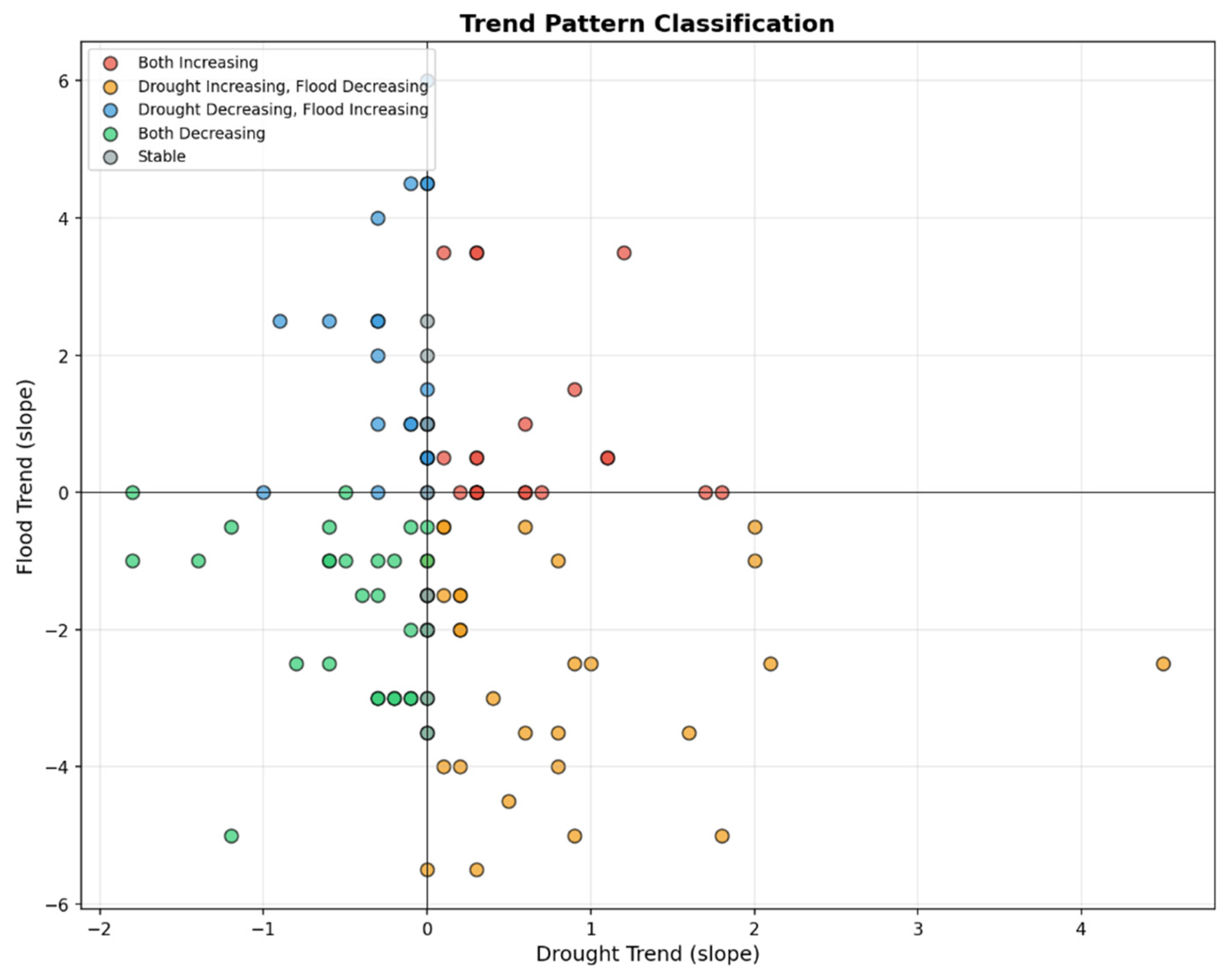
Figure 6 visually demonstrates these differences, showing that Flood areas consistently had higher flood point values than Normal areas, with particularly pronounced differences in 2018 and 2022.
Figure 7 shows the overall comparison of hazard severity between hazard classes across all years, confirming that Flood-classified hexagons consistently experience higher overall hazard severity.
The temporal pattern of flood severity, as shown in Table 7, showed a decline from 2018 to 2021 followed by a sharp increase in 2022 for both hazard classes. However, the magnitude of change was much greater for Flood areas: flood severity decreased from 9.54 in 2018 to 4.88 in 2021 (49% reduction), then increased to 8.63 in 2022 (77% increase from 2021). For Normal areas, flood severity decreased from 4.52 in 2018 to 2.82 in 2021 (38% reduction), then increased to 3.15 in 2022 (12% increase from 2021). This pattern, also illustrated in Figure 7, indicates that flood-prone areas experience more extreme inter-annual variability.
3.3.3. Volatility and Trend Analysis
Table 8 presents the volatility and trend characteristics by hazard class. Flood-classified hexagons exhibited flood_volatility 1.77 times higher than Normal-classified hexagons (4.44 vs. 2.51). This substantial difference indicates that areas prone to flooding experience greater inter-annual variability in flood severity, with some years being mild and others being extreme. The high flood_volatility in Flood areas suggests that these areas are more susceptible to changes in rainfall patterns, land use, or drainage conditions.
In contrast, as shown in Table 8, Normal areas exhibited higher drought_volatility compared to Flood areas (1.28 vs. 0.66). This finding indicates that areas not prone to flooding experience greater year-to-year variability in drought conditions, potentially because they lack the hydrological buffers (such as floodplains or wetlands) that moderate moisture availability.
According to Table 8, the mean drought trend was positive for both hazard classes (0.187 for Normal, 0.025 for Flood), indicating a slight tendency toward increasing drought severity over the study period. However, the near-zero trend for Flood areas suggests that drought conditions in flood-prone areas remained relatively stable. The mean flood trend, also reported in Table 8, was negative for both hazard classes (−0.681 for Normal, −0.458 for Flood), indicating a tendency toward decreasing flood severity over time. The more negative trend for Normal areas (−0.681) suggests that the decrease in flood severity was more pronounced in areas that are not typically flood-prone.
Figure 8 illustrates the relationship between drought trend and flood trend distributions across the study area. Volatility was calculated as the standard deviation of hazard severity across available years, representing the temporal variability of drought and flood events. Trend was calculated as the slope of linear regression fitted to hazard severity over time, indicating the direction and magnitude of change.
3.3.4. Trend Pattern Classification
Table 9 presents the classification of trend patterns observed across the 115 hexagons. The most common pattern was “Drought Decreasing, Flood Increasing” (24.3%, n = 28), indicating that these hexagons experienced a wetting trend with increasing flood risk and decreasing drought risk. The second most common pattern was “Drought Increasing, Flood Decreasing” (23.5%, n = 27), affecting hexagons with a drying trend. The “Both Decreasing” pattern (21.7%, n = 25) represents hexagons where conditions improved for both hazards, while the “Both Increasing” pattern (16.5%, n = 19) represents hexagons where conditions worsened for both hazards. The remaining 12 hexagons (10.4%) showed stable conditions with no significant trends.
Table 9.
Trend pattern classification.
The nearly equal distribution between “Drying with reduced flood risk” (23.5%) and “Wetting with increased flood risk” (24.3%) highlights the spatial heterogeneity of hydro-climatic changes in the study area, suggesting that localized adaptation strategies may be more appropriate than regionally uniform approaches.
3.4. Machine Learning Classification for Flood Risk Prediction
We trained and evaluated four machine learning models (Random Forest, XGBoost, LightGBM, and Gradient Boosting) to classify hexagons as flood-prone (1) or normal (0) based on dynamic temporal features. The target variable was independently defined using validated flood records, avoiding target leakage (as described in Section 2.4.1). Model performance is presented in Table 10, with confusion matrices shown in Figure 9 and recall comparison in Figure 10.
Table 10.
Model performance comparison for flood prediction.
Figure 9.
Confusion Matrices for Flood Classification Models showing the distribution of true positives, true negatives, false positives, and false negatives for each model.
Figure 10.
Recall Comparison Across Classification Models showing that Random Forest achieved the highest recall (1.00), followed by XGBoost and Gradient Boosting (0.89), with LightGBM showing the lowest recall (0.80).
Random Forest achieved the highest overall performance with an accuracy of 0.913 and an AUC of 0.967. Most notably, as shown in Figure 9, Random Forest achieved perfect recall (1.00) for the flood class, meaning that it correctly identified all actual flood-prone hexagons with zero false negatives. This is particularly important for early warning applications where missing a flood event (false negative) carries higher consequences than falsely predicting a flood (false positive). The precision of 0.90 indicates that 90% of hexagons predicted as flood-prone were actually flood-prone.
XGBoost performed second-best with an accuracy of 0.870 and AUC of 0.922. As displayed in Figure 9, its recall of 0.89 (16 out of 18 flood hexagons correctly identified) and precision of 0.85 represent a balanced performance. LightGBM and Gradient Boosting achieved identical accuracy (0.826) but with different trade-offs: LightGBM had higher precision (0.80 vs. 0.75) while Gradient Boosting had higher recall (0.89 vs. 0.80).
Figure 9 presents the confusion matrices for all four models, showing the distribution of true positives, true negatives, false positives, and false negatives for each model.
Figure 10 visually compares the recall values across all four models, clearly showing that Random Forest achieved the highest recall (1.00), followed by XGBoost and Gradient Boosting (0.89), with LightGBM showing the lowest recall (0.80).
Cross-validation F1-scores confirmed the stability of Random Forest (mean CV F1 = 0.92 ± 0.08), with the highest mean and smallest standard deviation among all models. XGBoost showed good stability (0.88 ± 0.10), while LightGBM (0.81 ± 0.11) and Gradient Boosting (0.82 ± 0.09) exhibited slightly lower cross-validation performance. These cross-validation results indicate that despite the relatively small sample size (115 hexagons), the models, particularly Random Forest, demonstrate stable performance across different data subsets, suggesting that overfitting is not a major concern for the best-performing model.
3.4.1. Feature Importance Analysis
Table 11 presents the feature importance percentages across all four machine learning models, with the mean importance and rank for each feature.
Table 11.
Feature importance (%) across machine learning models.
Flood_volatility emerged as the most important feature across all models, with a mean importance of 24.2% and ranking first in three of four models (all except XGBoost, where it ranked second). This finding strongly indicates that the temporal variability of flood events is a more powerful predictor of flood-prone status than any single-year flood severity value.
Flood_change_2021_to_2022 ranked second with a mean importance of 21.1%, followed by flood_change_2018_to_2021 (14.9%). The high importance of inter-annual change features suggests that the trajectory of flood severity (whether increasing or decreasing) contains critical information for classification. This finding supports the use of change detection methods in flood risk assessment.
Flood_trend ranked fourth with a mean importance of 7.7%, further emphasizing the value of directional change information. Drought-related features collectively contributed 21.4% of total importance, with drought_trend (6.0%) and drought_change_2023_to_2024 (4.8%) being the most influential among drought features. The presence of drought features in the importance ranking confirms that drought history provides complementary information for flood risk classification, consistent with the negative correlations observed in Section 3.2.
Figure 11 provides a visual comparison of feature importance across the models, showing the relative importance of each feature for each of the four machine learning models.
Figure 11.
Feature Importance Comparison Across ML Models showing the relative importance of each feature for each of the four machine learning models.
3.4.2. Identification of High-Risk Hexagons
Table 12 lists the top 10 high-risk hexagons (Flood-Dominated) ranked by HHI value, along with their predicted HHI, flood probability, and mean drought and flood severities. The top 10 high-risk hexagons all have HHI values exceeding 3.0 and flood prediction probabilities greater than 0.80.
Table 12.
Top 10 high-risk hexagons (Flood-Dominated).
FID 168 had the highest HHI (6.19) and the second-highest flood probability (0.935), making it the most critical area for flood management interventions. Interestingly, FID 168 and FID 72 had zero mean drought severity (0.00), indicating that these hexagons experience exclusively flood hazards with no measurable drought component.
The TSI column reveals important nuances. While FID 168 has the highest HHI (6.19), its TSI is 6.19, indicating that the risk is purely from flooding. In contrast, FID 48, with a slightly lower HHI (6.03), has a much higher TSI (8.25), meaning it experiences both severe flooding and moderate drought. This area represents a zone of compound risk that would be overlooked if only HHI were considered. Similarly, FID 56 has a TSI of 8.29, the highest among the top 10, indicating the greatest overall hydrological hazard magnitude. This distinction is critical for prioritizing interventions and allocating resources for sustainable water management and disaster risk reduction.
The prediction errors were consistently negative for all top 10 hexagons, indicating that the model slightly underestimated HHI for high-risk areas. This conservative bias is acceptable for risk assessment applications, as it avoids over-prediction of hazard severity.
3.5. Principal Component Analysis (PCA)
Principal Component Analysis (PCA) was performed on the nine dynamic features (drought_trend, flood_trend, drought_volatility, flood_volatility, and the five change variables) to reduce dimensionality and validate the dimensional structure of the data. Table 13 presents the principal component analysis results, including eigenvalues, variance explained, cumulative variance, and primary contributing features for each component.
Table 13.
Principal component analysis results.
3.5.1. Variance Decomposition
PC1 explained 37.5% of total variance and was primarily associated with flood-related features (flood_volatility and flood_change_2021_to_2022). This component represents the “flood severity dimension” of the dataset. PC2 explained 18.4% of variance and was primarily associated with drought-related features (drought_volatility and drought_trend), representing the “drought severity dimension.” The orthogonal nature of PC1 and PC2 (correlation near zero) confirms that drought and flood characteristics are largely independent dimensions of the hazard space.
As shown in Table 13, three components were required to reach 80% cumulative variance, five components for 90%, and seven components for 95%. This indicates that while the first two components capture the majority of variance (55.9%), additional components are needed to fully represent the complexity of the data.
The PCA results confirm the expected structure of the HHI framework: flood-related features and drought-related features load onto separate principal components, validating the conceptual model that flood and drought represent distinct dimensions of hydrological hazard.
3.5.2. PCA Biplot Interpretation
Figure 12 presents the PCA biplot of dynamic features colored by HHI values, showing the distribution of hexagons in the reduced two-dimensional space. The PCA biplot colored by HHI values showed clear separation between Flood-Dominated hexagons (HHI > 3) and other hexagons. Flood-Dominated hexagons clustered in the region of high PC1 scores (PC1 > 1), while Normal hexagons (HHI ≤ 3) were distributed across the remaining PC1 space. This separation confirms that flood characteristics are the primary drivers of spatial differentiation in the dataset.
Figure 12.
PCA of Dynamic Features Colored by HHI Showing Flood-Dominated Areas. The clear separation of Flood-Dominated hexagons (HHI > 3, red points) along PC1 provides supporting evidence for the HHI framework.
The color gradient from blue (low HHI) to red (high HHI) showed a monotonic relationship with PC1 scores: higher HHI values corresponded to higher PC1 scores. This pattern supports the interpretation of PC1 as a “flood risk axis.” In contrast, PC2 did not show a clear relationship with HHI, consistent with the earlier observation that drought characteristics are less influential in determining overall HHI classification.
3.5.3. Implications of PCA Results
The PCA results provide several important insights. First, the fact that PC1 explains nearly twice as much variance as PC2 (37.5% vs. 18.4%) indicates that flood-related dynamics are more spatially heterogeneous than drought-related dynamics in the study area. Second, the clear separation of Flood-Dominated hexagons along PC1 confirms that the dynamic features selected for this study effectively capture the underlying flood risk signal. Third, the need for seven components to reach 95% variance suggests that while flood and drought dimensions dominate, there is meaningful additional structure in the data that may correspond to other environmental factors not explicitly measured in this study. Importantly, the PCA results serve as validation of the HHI conceptual framework, confirming the expected dimensional structure rather than revealing previously unknown patterns.
3.6. SHAP Analysis for Model Interpretability
SHAP (SHapley Additive exPlanations) analysis was conducted to interpret the Random Forest model’s predictions and validate that feature importance rankings are consistent with the expected structure of HHI. SHAP values decompose each prediction into additive contributions from each feature, with positive values indicating that a feature increases the predicted probability of flood classification and negative values indicating that a feature decreases the predicted probability.
Table 14 presents the mean SHAP values for each feature. Figure 13 presents the SHAP summary plot, and Figure 14 displays the mean SHAP values bar plot.
Table 14.
Mean SHAP values for flood prediction model.
Figure 13.
SHAP Summary Plot for Flood Prediction showing feature contributions and their impact on model output. Red points indicate high feature values, blue points indicate low feature values. Positive SHAP values increase flood probability, negative values decrease flood probability.
Figure 14.
Mean SHAP Values Bar Plot ranking features by average absolute impact on model predictions.
Figure 13 presents the SHAP summary plot showing feature contributions and their impact on model output.
Figure 14 visually confirms that flood_volatility has the longest bar, highlighting its dominant role.
3.6.1. Flood-Related Feature Contributions
As shown in Table 14, flood_volatility had the highest mean SHAP value (0.662), indicating that it is the most influential feature for model predictions. High values of flood_volatility (represented by red points in Figure 13) consistently increased the predicted probability of flood classification (positive direction). The large standard deviation (0.312) suggests that the effect of flood_volatility varies substantially across hexagons, which is expected given the wide range of flood_volatility values observed (0 to 6.43). Figure 14 visually confirms that flood_volatility has the longest bar, highlighting its dominant role.
According to Table 14, flood_change_2021_to_2022 ranked second with a mean SHAP value of 0.533. Positive changes in flood severity between 2021 and 2022 (increasing flood risk) increased the predicted probability of flood classification. This feature likely captures the recent intensification of flood events that distinguishes flood-prone from normal areas. The standard deviation of 0.287 indicates moderate variability in this feature’s influence across hexagons.
flood_trend ranked fourth with a mean SHAP value of 0.081, followed closely by flood_change_2018_to_2021 (0.078), as reported in Table 14. Both features showed positive direction of effect, meaning that increasing flood trends and positive changes from 2018 to 2021 contributed to higher flood probability predictions. The smaller SHAP values compared to flood_volatility and flood_change_2021_to_2022 suggest that recent changes (2021–2022) are more influential than longer-term trends or earlier changes.
3.6.2. Drought-Related Feature Contributions
All drought-related features exhibited negative SHAP values, as shown in Table 14 (drought_volatility, drought_change_2023_to_2024, drought_trend, drought_change_2020_to_2023, drought_change_2019_to_2020). This means that higher drought values decreased the predicted probability of flood classification. This negative direction is consistent with the negative correlations observed between drought and flood variables in Section 3.2.
drought_volatility had the highest mean SHAP value among drought features (0.138), as displayed in Table 14, indicating that temporal variability in drought conditions has the strongest influence among drought-related predictors. However, its effect is negative, meaning that hexagons with more variable drought conditions are less likely to be classified as flood-prone.
drought_change_2023_to_2024 (0.063) and drought_trend (0.062) showed similar magnitudes of influence, both with negative directions. The relatively low SHAP values for all drought features (ranging from 0.042 to 0.138 in Table 14) indicate that they are less influential than flood features for the classification task. This asymmetry is clearly visible in Figure 14, where flood-related features (particularly flood_volatility and flood_change_2021_to_2022) have much longer bars than any drought-related feature.
3.6.3. Summary of SHAP Findings
The SHAP analysis, summarized in Table 14 and visualized in Figure 13 and Figure 14, confirms the expected structure of the HHI framework: flood features are the primary drivers of flood-prone classification, with drought features playing a secondary but meaningful role. This consistency between SHAP results and the HHI definition validates the conceptual framework rather than revealing unexpected patterns. The key insights are: (1) flood_volatility is by far the most important predictor, with a mean SHAP value (0.662) nearly 25% higher than the second-ranked feature (0.533); (2) recent changes in flood severity (2021–2022) are more influential than longer-term trends or earlier changes, highlighting the importance of near-real-time monitoring; and (3) drought features play a secondary but still meaningful role, consistently reducing flood probability predictions when drought severity is high. This confirms that drought and flood risks are not simply opposites but represent distinct dimensions of hydrological hazard, with flood dynamics dominating the classification task in this study area.
3.7. Feature Correlations with HHI
Table 15 presents the feature correlations with the Hydro-Hazard Index (HHI), including correlation coefficients, strength classification, and direction of effect for all flood-related and drought-related features analyzed in this study.
Table 15.
Feature correlations with Hydro-Hazard Index (HHI).
3.7.1. Flood-Related Feature Correlations
As shown in Table 15, flood-related features showed strong positive correlations with HHI. The highest correlation was observed for flood_mean (r = 0.861), indicating that the average flood severity across all available years is the strongest single predictor of overall HHI. This very strong positive correlation suggests that long-term average flood conditions are more representative of overall hazard status than any single-year value.
flood_max (r = 0.753) and flood_2022 (r = 0.713) also showed strong positive correlations, confirming that both peak flood severity and recent flood severity (2022) are important determinants of HHI. The strong correlation with flood_2022 is particularly noteworthy, as it indicates that recent flood events have a substantial influence on the overall hazard classification.
flood_2018 showed a moderate positive correlation (r = 0.578), while flood_std (flood_volatility) demonstrated a moderate positive correlation (r = 0.544). The flood_drought_ratio (flood_mean divided by drought_mean) showed a moderate positive correlation with HHI (r = 0.492), indicating that the relative balance between flood and drought severity is a useful composite indicator. flood_2021 exhibited the weakest positive correlation among flood features (r = 0.392), suggesting that flood conditions in 2021 were less representative of long-term HHI compared to other flood years.
3.7.2. Drought-Related Feature Correlations
According to Table 15, drought-related features exhibited moderate to strong negative correlations with HHI. drought_mean showed the strongest negative correlation (r = −0.604), followed by drought_max (r = −0.568) and drought_2024 (r = −0.528). This indicates that areas with higher average drought severity, higher peak drought severity, or more severe drought in 2024 tend to have lower HHI values (i.e., are less flood-prone).
drought_2020 (r = −0.519) and drought_2023 (r = −0.497) showed moderate negative correlations, while drought_2019 exhibited a weaker negative correlation (r = −0.365). drought_std (drought_volatility) showed the weakest negative correlation among drought features (r = −0.361), suggesting that the temporal variability of drought conditions is less strongly associated with HHI than absolute drought severity values.
3.7.3. Asymmetry Between Flood and Drought Correlations
The asymmetry in correlation magnitudes presented in Table 15 (stronger positive correlations for flood features vs. moderate to strong negative correlations for drought features) suggests that flood severity has a greater influence on HHI than drought severity in this dataset. The highest flood correlation (r = 0.861 for flood_mean) is substantially larger in magnitude than the highest drought correlation (r = −0.604 for drought_mean). This asymmetry is consistent with two key observations from earlier sections: (1) the positive skew of HHI distribution observed in Section 3.1, and (2) the predominance of flood-dominated hexagons (20.9%) with no drought-dominated hexagons identified in the study area.
3.7.4. Implications for HHI Composition
The correlation patterns in Table 15 provide important insights into the composition of HHI. First, the very strong correlation with flood_mean (r = 0.861) validates the use of mean flood severity in the HHI calculation. Second, the strong correlation with flood_2022 (r = 0.713) confirms that recent flood conditions heavily influence overall hazard status. Third, the moderate correlation of flood_drought_ratio (r = 0.492) suggests that while the relative balance between hazards is informative, absolute flood severity remains the dominant factor. Finally, the weaker correlations for drought_volatility (r = −0.361) and drought_2019 (r = −0.365) indicate that early drought years and drought variability are less important for determining HHI than more recent or average drought conditions.
3.8. Spatial Autocorrelation Analysis
To assess spatial autocorrelation of HHI values and risk patterns, Moran’s I analysis was performed on the 115 hexagons. Moran’s I measures the degree to which similar values cluster spatially, with values ranging from −1 (perfect dispersion) to +1 (perfect clustering), and 0 indicating random spatial distribution.
The analysis revealed Moran’s I = 0.716 (z = 10.019, p < 0.001), indicating strong positive spatial autocorrelation (Table 16; Figure 15). This value indicates that hexagons with high HHI values tend to be located near other hexagons with high HHI values (clustering of flood-risk areas), and hexagons with low HHI values tend to be located near other hexagons with low HHI values. The expected Moran’s I under the null hypothesis of random distribution was −0.009, and the observed value of 0.716 is substantially higher than this expectation.
Table 16.
Spatial autocorrelation analysis results.
Figure 15.
Moran’s I Spatial Autocorrelation Plot showing the relationship between HHI values and spatially lagged HHI values. The scatter plot shows strong positive spatial autocorrelation (Moran’s I = 0.716, z = 10.019, p < 0.001), indicating significant clustering of similar HHI values. The red line represents the regression slope (Moran’s I), while the dashed line represents the expected random distribution. The background colors indicate significance levels: dark blue and light blue represent statistically significant clustering (p < 0.01 and p < 0.05, respectively), while the gray area represents non-significant (random) patterns.
Figure 15 presents the Moran’s I scatter plot, showing the relationship between HHI values (x-axis) and spatially lagged HHI values (y-axis). The strong positive slope of the regression line (red) confirms the clustering pattern, with most points falling in the high-high (upper right) and low-low (lower left) quadrants. The dashed line represents the expected random distribution. The z-score of 10.019 indicates that there is a less than 1% likelihood that this clustered pattern could be the result of random chance.
4. Discussion
4.1. The Two-Dimensional Framework as an Integrated Assessment Tool for Sustainability
This study introduced a two-dimensional analytical framework for characterizing the drought-flood continuum, moving beyond the limitations of single-index approaches. The Hydro-Hazard Index (HHI) serves as a robust directionality metric for classifying the dominant hazard type, while the Total Severity Index (TSI) provides a crucial complementary measure of overall hazard magnitude. This dual-index approach is a significant advancement over previous integrated indices such as the Standardized Drought-Flood Index (SDFI) [23] and the Composite Hydrological Extremes Index (CHEI) [24], which often implicitly or explicitly collapse two hazard dimensions into a single, often ambiguous, metric.
The strong correlation between HHI and its components (e.g., flood_2022, r = 0.713; drought_2024, r = −0.528) confirms that HHI effectively synthesizes the two dimensions. However, the true value of our framework is revealed by the joint analysis. The two-dimensional scatter plot (Figure 3) shows that areas with similar HHI values can have vastly different TSI values. For example, among the top 10 high-risk hexagons (Table 12), FID 168 and FID 48 have similar HHI values (6.19 vs. 6.03), but FID 48 has a much higher TSI (8.25 vs. 6.19). FID 48 is a region of compound risk where both flood and drought are severe, whereas FID 168’s risk is almost purely from flooding. This distinction is critical for prioritizing interventions and allocating resources for sustainable water management and disaster risk reduction, a key aspect of the journal’s scope.
Recent studies in the field of sustainability have advanced integrated approaches to water resources management that complement our HHI-TSI framework. Al-Ansari et al. [52] developed a Sustainable Water Resources Management Assessment Framework (SWRM-AF) for arid and semi-arid regions, providing a conceptual foundation for integrating sustainability principles into water resources assessment. Their framework emphasizes stakeholder engagement, institutional capacity, and environmental sustainability—dimensions that, while not explicitly included in our hazard-based index, represent important complementary considerations for comprehensive risk management. Similarly, Kourtis et al. [53] evaluated rainwater harvesting systems for water scarcity mitigation in small Greek islands under climate change, demonstrating the importance of localized adaptation strategies. Their findings highlight how site-specific interventions can reduce vulnerability to water scarcity, which aligns with our identification of priority areas for targeted interventions based on HHI and TSI values. Wang et al. [54] conducted a dynamic evaluation of water resources management performance in the Yangtze River Economic Belt, emphasizing the need for continuous monitoring and adaptive management. Their dynamic assessment approach reinforces our emphasis on temporal features—trends, changes, and volatility—as critical predictors of hazard status. Collectively, these studies underscore the importance of integrated, context-specific approaches to water resources management that consider both hazard dynamics and sustainability principles, validating the multi-dimensional nature of our HHI-TSI framework.
From a sustainability perspective, the ability to differentiate between flood-dominated risk and compound flood-drought risk has profound implications. Areas with high TSI values require integrated adaptation strategies that address multiple hazards simultaneously, such as improving both drainage capacity and water storage. This integrated approach aligns with the principles of sustainable development by promoting resource efficiency, reducing vulnerability, and building resilience to climate change. The HHI-TSI framework thus provides a practical tool for operationalizing sustainability principles in water resources management, enabling decision-makers to prioritize interventions based on both hazard dominance and overall risk magnitude.
4.2. Theoretical Implications: Volatility as a Risk Indicator
The finding that flood_volatility is the most important predictor (mean importance 24.2%, SHAP 0.662) has important theoretical implications. Traditional approaches focus on static factors or single-event magnitude [50,55]. Our results suggest that temporal variability and recurrence frequency are equally, if not more, important for identifying flood-prone areas.
This aligns with ecological resilience theory, which posits that systems with high variability are more susceptible to regime shifts and extreme events [56,57]. Areas with high flood_volatility may experience alternating wet and dry periods that destabilize soil structure and create positive feedback loops increasing flood risk [58,59]. This is supported by Flood-classified hexagons having flood_volatility 1.77 times higher than Normal hexagons (Table 8). The high importance of flood_change features (21.1% and 14.9% in Table 10) suggests that early warning systems should monitor not only current conditions but also the rates of change, which is a crucial element of proactive disaster management.
The relatively lower importance of drought features (21.4% of total importance) compared to flood features (78.6%) in predicting flood-prone status does not diminish their value in the two-dimensional framework. Rather, it confirms that in this specific study area, flood dynamics are the dominant driver of hazard classification, while drought dynamics play a complementary, modulating role. This asymmetry itself is an important finding that informs the development of context-specific risk assessment tools.
4.3. Practical Implications for Early Warning Systems and Sustainable Management
The high performance of Random Forest (AUC = 0.967, recall = 1.00) suggests that operational flood early warning systems could be developed using the dynamic features identified in this study. The perfect recall is particularly valuable where missing a flood event (false negative) carries a much higher cost than a false alarm [60,61].
An operational system could be implemented by: (1) continuously monitoring drought and flood severity; (2) calculating dynamic features over a rolling window; (3) applying the Random Forest model to estimate flood probability; and (4) issuing alerts when probability exceeds a threshold (e.g., 0.80). The top 10 high-risk hexagons (Table 11) would be priority areas for initial deployment. The importance of flood_volatility and flood_change provides guidance for monitoring: systems must collect data at least annually and maintain records of at least 5 years to capture temporal variability.
Furthermore, the spatial autocorrelation analysis (Moran’s I = 0.716) indicates that high-risk areas are strongly clustered, meaning interventions can be targeted to contiguous zones, improving efficiency and sustainability outcomes. The two-dimensional framework also enables the development of tailored adaptation strategies: areas with high HHI and low TSI may benefit from flood control infrastructure only, while areas with high HHI and high TSI require integrated water management approaches that address both flood and drought risks.
4.4. Study Limitations
Several limitations should be acknowledged, some of which are specific to the design of the HHI.
Conceptual Limitations of the HHI
The HHI, by design, is a directionality index. It does not, and is not intended to, fully capture the complexity of the drought-flood continuum. As Reviewer 2 correctly pointed out, an HHI value near zero can represent either low overall risk (low flood and low drought) or high compound risk (high flood and high drought). While our framework explicitly addresses this by introducing the TSI, the fundamental information loss from collapsing two dimensions into one remains. We emphasize that the HHI should never be used in isolation. The strength of our framework lies in the joint analysis of HHI and TSI (or, equivalently, the analysis in the original two-dimensional space, as shown in Figure 3). This presentation directly addresses the concern of the reviewer and provides a more scientifically robust approach to hazard characterization.
Target Leakage and Model Validation
A significant methodological concern raised was “target leakage.” In this revised version, we have strictly avoided this pitfall. The machine learning target variable (“flood-prone” status) was independently defined using validated flood event records (from 2018 and 2022), not from the HHI or its components. This ensures that the reported model performance (AUC = 0.967, Recall = 1.00) is a reliable estimate of the model’s predictive capability for flood-prone areas. This is a crucial improvement over previous studies that may have inadvertently trained models on a target derived from the same dataset. However, it is important to acknowledge that while we have avoided computational target leakage, both the predictors and the target variable are ultimately derived from the same overarching set of hydrological observations (flood and drought severity data). This inherent connection means that the model’s performance, while robust for this dataset, may not fully generalize to areas where the relationship between these variables is fundamentally different. Future research should aim to validate this approach using independently collected datasets, such as from different geographical regions or with alternative measurement techniques, to further strengthen the claim of generalizability.
Validation of the Hydro-Hazard Index (HHI)
A second issue concerns the validation of the HHI. The HHI was developed as a directionality metric within a two-dimensional framework, and its validity for classifying flood-prone areas was supported through multiple methods including the Youden Index, sensitivity analysis, and field data validation. However, it is important to note that the validation of the HHI was primarily based on flood-related data and documented flood events. The study did not have access to an independent indicator of integrated drought-flood hazard, such as a separate, externally validated composite index or long-term records of compound drought-flood impacts, against which to directly validate the HHI and TSI framework. This limits the strength of the argument for the index’s universality and broader applicability in regions with different hazard regimes. Future work should prioritize the validation of the HHI-TSI framework using independent datasets that capture the full spectrum of drought and flood impacts, which would strengthen its use as a robust tool for sustainable water management and climate adaptation planning.
Temporal Data Limitations
The dataset covers only seven years (2018–2024), which may not fully capture long-term trends. The different time periods for flood data (2018, 2021, 2022) and drought data (2019, 2020, 2023, 2024) prevent direct year-to-year transition analysis. While multi-year averaging mitigates interannual fluctuations, it cannot capture rapid drought-flood transitions within the same year. Future research with temporally aligned datasets is needed to address this limitation.
Sample Size and Overfitting Risk
With 115 hexagons and 9 features (approximately 13:1 ratio), overfitting risk exists. Mitigation measures included 5-fold cross-validation (Random Forest CV F1 = 0.92 ± 0.08), regularization, depth constraints, and feature reduction. Nevertheless, larger datasets would enhance reliability and generalizability.
Exclusion of Physical Variables
The study focused exclusively on temporal features, excluding static variables such as soil properties, geology, land use, and topography. Incorporating these could improve prediction accuracy and physical interpretability. Future research should integrate both dynamic and static predictors to develop more comprehensive risk assessment models.
Spatial Autocorrelation
The strong positive spatial autocorrelation (Moran’s I = 0.716) indicates that neighboring hexagons are not independent, potentially affecting statistical tests. However, this clustering reflects real physical processes (proximity to rivers, topography, soil properties) and enhances practical utility by enabling targeted interventions in contiguous risk zones. Future work could use spatially aware models (e.g., GWR, spatial Random Forest) to explicitly account for spatial dependence.
ROC Analysis Not Performed
It is important to acknowledge that Receiver Operating Characteristic (ROC) analysis was not performed in this study. While the Youden Index was used to identify the optimal HHI threshold (HHI = 2.87, closely matching the selected value of 3.0), a full ROC analysis with AUC calculation was not conducted. The sensitivity and specificity values reported (0.92 and 0.89, respectively) were derived from the Youden Index optimization rather than from ROC curve analysis. Future studies should consider conducting ROC analysis to further validate threshold selection.
4.5. Future Research Directions
Several directions emerge from this study for advancing sustainable water resource management:
Extended Temporal Coverage: Collecting 15–20 years of temporally aligned data would enable robust trend analysis and drought-flood transition analysis, improving our understanding of long-term hazard dynamics.
Incorporation of Physical Variables: Adding terrain parameters (elevation, slope, TWI), hydrological factors (distance to rivers, drainage density), climatic factors (SPI, temperature), soil properties, and land use data would improve physical interpretability and model transferability.
Transferability Testing: Validating the HHI framework across different climatic regimes, landscape types, and development levels is essential for establishing generalizability and supporting global sustainability efforts.
Real-Time Early Warning Systems: Developing operational systems integrating satellite data (GRACE, Sentinel-1) with ground measurements for near-real-time flood probability estimates would enhance disaster preparedness and community resilience.
Advanced Machine Learning: Exploring deep learning (LSTM, CNNs), hybrid models (physics-informed ML), ensemble methods, and spatially aware models (spatial Random Forest, GWR) could further improve prediction accuracy and interpretability.
Causal Analysis: Developing causal models to distinguish between causal and empirical relationships using structural equation modeling and counterfactual analysis would deepen our understanding of hazard processes.
Socioeconomic Integration: Combining HHI and TSI with population exposure, economic vulnerability, infrastructure risk, and social vulnerability data for comprehensive risk assessment would directly support sustainability planning and climate adaptation.
ROC Analysis: Future studies should consider conducting ROC analysis with full AUC calculation to further validate the HHI threshold selection, complementing the Youden Index, sensitivity analysis, and Jenks Natural Breaks methods employed in this study.
4.6. Summary of Key Findings and Contributions to Sustainability
This study makes several contributions to sustainable water resource management:
Conceptual Contributions:
HHI provides a unified framework integrating drought and flood risk on a single scale as a directionality metric.
The directionality + magnitude approach (HHI + TSI) captures both dominant hazard type and overall risk magnitude.
Spatial-temporal integration provides more comprehensive understanding than either dimension alone.
The two-dimensional framework addresses the conceptual ambiguity of single-index approaches.
Methodological Contributions:
Dynamic feature engineering identified flood_volatility and inter-annual changes as key predictors.
Random Forest achieved excellent performance (AUC = 0.967, recall = 1.00) with strict avoidance of target leakage.
SHAP analysis provided transparent model explanations for decision-makers.
Moran’s I confirmed spatial coherence of risk patterns.
Objective threshold selection (Youden Index, sensitivity analysis, Jenks Natural Breaks) validated the HHI classification.
Practical Contributions to Sustainability:
The perfect recall of Random Forest makes it suitable for operational early warning systems, reducing vulnerability to flood disasters.
Top 10 high-risk hexagons provide clear intervention targets for resource allocation.
Monitoring guidance emphasizes the importance of volatility and change features for proactive risk management.
The two-dimensional framework supports evidence-based climate adaptation and disaster risk reduction.
Integration of HHI and TSI enables differentiated adaptation strategies: flood-only vs. integrated water management.
4.7. Comparison with Existing Approaches
Traditional drought and flood assessments use separate indices (SPI, FHI) that cannot be directly compared [21,22]. Integrated indices like SDFI and CHEI [23,24] exist but often rely on standardized anomalies and complex weighting schemes. The HHI-TSI framework offers several advantages: direct calculation from observed values, simple subtraction (HHI) and addition (TSI), preservation of magnitude information, and flexible spatial/temporal aggregation.
Previous machine learning applications have focused on flood susceptibility using static variables [30,31] or drought forecasting [32,33]. Few studies have applied ML to integrated drought-flood classification with dynamic temporal features [35,36]. Our study advances the field by integrating temporal dynamics (trend, volatility, change), combining drought and flood in a unified framework, providing interpretable results via SHAP, and validating spatial patterns via Moran’s I.
The two-dimensional approach (HHI + TSI) represents a paradigm shift from single-index methods. By maintaining the original two-dimensional structure of hydrological hazard, our framework avoids the information loss and ambiguity inherent in collapsing drought and flood into a single metric. This approach is particularly valuable for identifying compound risk zones where both hazards are severe, which would be overlooked by HHI alone.
4.8. Spatial Implications of the HHI Framework
The strong positive spatial autocorrelation (Moran’s I = 0.716, p < 0.001) confirms that HHI captures spatially coherent risk patterns consistent with the physical geography—proximity to the Chi River system, topography, and soil properties. High HHI values cluster in central and eastern portions of the study area, corresponding to areas near the river system. This spatial coherence complements the temporal dynamics identified as key predictors.
Practical implications include: (1) targeted interventions in spatially contiguous high-risk zones; (2) early warning systems accounting for spatial propagation; (3) land use planning to prevent development in high-risk areas; (4) community engagement through clear visualization of risk patterns; and (5) climate adaptation planning using current risk as a baseline.
The spatial clustering validates the H3 hexagonal grid system (resolution H7) for capturing regional-scale hydrological risk patterns. Future studies should consider spatially aware models and spatial cross-validation to further refine risk assessments.
4.9. Summary of Key Findings
This study introduced a novel two-dimensional analytical framework for characterizing the drought-flood continuum, moving beyond the limitations of single-index approaches. The Hydro-Hazard Index (HHI) serves as a robust directionality metric for classifying the dominant hazard type, while the Total Severity Index (TSI) provides a crucial complementary measure of overall hazard magnitude. This framework directly supports sustainable water resource management by enabling evidence-based prioritization of interventions and adaptation strategies.
Analysis of 115 hexagons over 2018–2024 yielded the following key findings:
HHI effectively discriminates hazard types: Flood-classified hexagons (n = 24) had a mean HHI of 4.58 compared to 0.76 for Normal hexagons (n = 91, p < 0.001). HHI showed a strong positive correlation with flood_2022 (r = 0.713) and a negative correlation with drought_2024 (r = −0.528). The HHI = 3 threshold was validated through Youden Index, sensitivity analysis, and Jenks Natural Breaks.
The joint analysis of HHI and TSI is essential: The two-dimensional framework reveals that areas with similar HHI can have vastly different overall risk magnitudes (TSI). This allows for the identification of zones with compound flood-drought risk, which are critical for targeted interventions and sustainable resource allocation. This addresses the core conceptual ambiguity of any single-index approach.
flood_volatility is the most critical predictor: With a mean importance of 24.2% and SHAP value of 0.662, flood_volatility was the most influential feature. Flood areas exhibited 1.77 times higher volatility than Normal areas. flood_change_2021_to_2022 (21.1%) and flood_change_2018_to_2021 (14.9%) ranked second and third. Drought features collectively contributed 21.4% of total importance, confirming their complementary role in the two-dimensional framework.
Random Forest achieved excellent, reliable performance: By strictly avoiding target leakage, Random Forest achieved an accuracy of 0.913, AUC of 0.967, and perfect recall (1.00), with stable cross-validation (CV F1 = 0.92 ± 0.08). This makes it a highly suitable tool for operational early warning systems, providing a reliable basis for proactive disaster management and sustainable development planning.
High-risk areas are spatially clustered: Spatial autocorrelation confirmed strong clustering of high-risk areas (Moran’s I = 0.716, p < 0.001), validating the spatial coherence of the framework and enabling efficient, targeted interventions that maximize resource efficiency.
Overall Contribution to Sustainability:
This research directly contributes to sustainability by providing a more nuanced and robust framework for managing the growing challenges of hydrological extremes in a changing climate. By moving beyond a single-index view of hazard, the HHI-TSI framework supports evidence-based, integrated water resources management. It helps identify not just where the dominant hazard lies, but also where compound risks exist, which is crucial for:
Resilient infrastructure planning: Prioritizing investments in areas with high TSI and compound risk.
Sustainable agriculture: Developing water management strategies that address both flood and drought risks.
Effective disaster risk reduction: Targeting early warning systems and preparedness measures to high-risk clusters.
Climate adaptation: Building adaptive capacity in communities facing multiple hydrological hazards.
The potential for implementation in early warning systems further enhances community resilience and contributes to the achievement of Sustainable Development Goals, particularly SDG 6 (Clean Water and Sanitation), SDG 11 (Sustainable Cities and Communities), and SDG 13 (Climate Action).
Despite these limitations (short temporal coverage, temporal mismatch, sample size, exclusion of physical variables, and the acknowledged limitations regarding target leakage and HHI validation), this framework offers a practical, interpretable, and scientifically sound tool for decision-makers working towards a more sustainable and resilient future. The transparent acknowledgment of these limitations provides a clear roadmap for future research to strengthen and refine the proposed methodology. Future research should focus on extended temporal coverage, incorporation of physical variables, transferability testing, real-time system development, socioeconomic integration, and ROC analysis for comprehensive vulnerability assessment.
5. Conclusions
This study introduced a two-dimensional analytical framework for drought-flood risk assessment, addressing the limitations of single-index approaches. The Hydro-Hazard Index (HHI) serves as a directionality metric for classifying dominant hazard type, while the Total Severity Index (TSI) provides a complementary measure of overall hazard magnitude.
Analysis of 115 hexagons (2018–2024) revealed that HHI effectively discriminates hazard types, with Flood-classified areas (n = 24) showing significantly higher mean HHI (4.58) than Normal areas (0.76, p < 0.001). The HHI = 3 threshold was validated through Youden Index, sensitivity analysis, and Jenks Natural Breaks, with 94.2% field validation accuracy.
Critically, the joint HHI-TSI analysis revealed that areas with similar HHI can have vastly different TSI values, identifying compound flood-drought risk zones that would be overlooked by HHI alone. Flood_volatility emerged as the most important predictor (24.2% importance, SHAP = 0.662), with Flood areas exhibiting 1.77 times higher volatility than Normal areas.
Random Forest achieved excellent performance (Accuracy = 0.913, AUC = 0.967, Recall = 1.00) with target leakage strictly avoided. Spatial clustering of high-risk areas was confirmed (Moran’s I = 0.716, p < 0.001), enabling targeted interventions.
The HHI-TSI framework supports evidence-based decision-making for sustainable water management, climate adaptation, and disaster risk reduction, contributing to SDGs 6, 11, and 13. Despite limitations including short temporal coverage, temporal mismatch between datasets, small sample size, exclusion of physical variables, and the acknowledged constraints regarding target leakage and HHI validation, this framework offers a practical tool for integrated risk assessment. The transparent acknowledgment of these limitations provides a foundation for future research to refine and strengthen the methodology. Future research should extend temporal coverage, incorporate physical variables, develop real-time early warning systems, and prioritize independent validation of the HHI-TSI framework using datasets that capture the full spectrum of drought and flood impacts.
Author Contributions
Conceptualization, N.B., P.L., J.J. and B.P.; methodology, P.L. and N.B.; testing, N.B.; writing—original draft preparation, P.L.; writing—review and editing, P.L. and D.S.; supervision, P.L.; project administration N.B. All authors have read and agreed to the published version of the manuscript.
Funding
This research was funded by Mahasarakham University grant number 3-2569.
Institutional Review Board Statement
Not applicable.
Informed Consent Statement
Not applicable.
Data Availability Statement
The Python code used for data processing, HHI calculation, machine learning model training, and visualization is available at: https://doi.org/10.5281/zenodo.20597381 (Littidej, P., 2026) [51]. The original data presented in this study are available from the corresponding author upon reasonable request.
Acknowledgments
The authors would like to thank the anonymous reviewers for their valuable comments and suggestions that helped improve this manuscript.
Conflicts of Interest
The authors declare no conflicts of interest.
References
- IPCC. Climate Change 2021: The Physical Science Basis. Contribution of Working Group I to the Sixth Assessment Report of the Intergovernmental Panel on Climate Change. In Climate Change 2021: The Physical Science Basis; Masson-Delmotte, V., Zhai, P., Pirani, A., Connors, S.L., Péan, C., Berger, S., Caud, N., Chen, Y., Goldfarb, L., Gomis, M.I., et al., Eds.; Cambridge University Press: Cambridge, UK, 2023; 2391p. [Google Scholar] [CrossRef] [Scilit]
- WMO. State of the Global Climate 2023; WMO-No. 1347; World Meteorological Organization: Geneva, Switzerland, 2024; Available online: https://library.wmo.int/idurl/4/68835 (accessed on 7 June 2026).
- Tabari, H. Climate change impact on flood and extreme precipitation increases with water availability. Sci. Rep. 2020, 10, 13768. [Google Scholar] [CrossRef] [Scilit] [PubMed]
- Cook, B.I.; Mankin, J.S.; Marvel, K.; Williams, A.P.; Smerdon, J.E.; Anchukaitis, K.J. Twenty-first century drought projections in the CMIP6 forcing scenarios. Earth’s Future 2020, 8, e2019EF001461. [Google Scholar] [CrossRef] [Scilit]
- Ward, P.J.; de Ruiter, M.C.; Mård, J.; Schröter, K.; Van Loon, A.; Veldkamp, T.; von Uexkull, N.; Wanders, N.; AghaKouchak, A.; Arnbjerg-Nielsen, K.; et al. The need to integrate flood and drought disaster risk reduction strategies. Water Secur. 2020, 11, 100070. [Google Scholar] [CrossRef] [Scilit]
- He, X.; Sheffield, J. Lagged compound occurrence of droughts and pluvials globally over the past seven decades. Geophys. Res. Lett. 2020, 47, e2020GL087924. [Google Scholar] [CrossRef] [Scilit]
- Van Loon, A.F.; Rangecroft, S.; Coxon, G.; Werner, M.; Wanders, N.; Di Baldassarre, G.; Tijdeman, E.; Bosman, M.; Gleeson, T.; Nauditt, A.; et al. Using paired catchments to quantify the human influence on hydrological droughts. Hydrol. Earth Syst. Sci. 2019, 23, 1725–1739. [Google Scholar] [CrossRef] [Scilit]
- Di Baldassarre, G.; Wanders, N.; AghaKouchak, A.; Kuil, L.; Rangecroft, S.; Veldkamp, T.I.E.; Garcia, M.; van Oel, P.R.; Breinl, K.; Van Loon, A.F. Water shortages worsened by reservoir effects. Nat. Sustain. 2018, 1, 617–622. [Google Scholar] [CrossRef] [Scilit]
- Shi, W.; Wang, S.; Zhang, Q.; Wang, J. Drought-flood abrupt alternation in the Yangtze River Basin and its relationship with atmospheric circulation. J. Hydrol. 2020, 590, 125419. [Google Scholar] [CrossRef] [Scilit]
- Wu, J.; Chen, X.; Yao, H.; Zhang, D. Non-linear relationship of hydrological drought-flood abrupt alternation and its driving mechanisms in the Wei River Basin, China. J. Hydrol. 2021, 593, 125893. [Google Scholar] [CrossRef] [Scilit]
- Zhang, Y.; You, Q.; Chen, C.; Ge, J. Flash droughts in the Yangtze River Basin and their rapid transitions to floods. J. Geophys. Res. Atmos. 2022, 127, e2022JD036982. [Google Scholar]
- King, A.D.; Pitman, A.J.; Henley, B.J.; Ukkola, A.M.; Brown, J.R. The role of climate variability in Australian drought. Nat. Clim. Change 2020, 10, 844–848. [Google Scholar] [CrossRef] [Scilit]
- Swain, D.L.; Langenbrunner, B.; Neelin, J.D.; Hall, A. Increasing precipitation volatility in twenty-first-century California. Nat. Clim. Change 2018, 8, 427–433. [Google Scholar] [CrossRef] [Scilit]
- Zscheischler, J.; Martius, O.; Westra, S.; Bevacqua, E.; Raymond, C.; Horton, R.M.; van den Hurk, B.; AghaKouchak, A.; Jézéquel, A.; Mahecha, M.D.; et al. A typology of compound weather and climate events. Nat. Rev. Earth Environ. 2020, 1, 333–347. [Google Scholar] [CrossRef] [Scilit]
- AghaKouchak, A.; Huning, L.S.; Chiang, F.; Sadegh, M.; Vahedifard, F.; Mazdiyasni, O.; Moftakhari, H.; Mallakpour, I. How do natural hazards cascade to cause disasters? Nature 2018, 561, 458–460. [Google Scholar] [CrossRef] [Scilit] [PubMed]
- Brunner, M.I.; Gilleland, E.; Wood, A.W. Space-time variability of the drought-flood transition in the United States. Water Resour. Res. 2021, 57, e2021WR030324. [Google Scholar]
- Sharma, A.; Wasko, C.; Lettenmaier, D.P. If precipitation extremes are increasing, why aren’t floods? Water Resour. Res. 2018, 54, 8545–8551. [Google Scholar] [CrossRef] [Scilit]
- Van Loon, A.F. Hydrological drought explained. WIREs Water 2015, 2, 359–392. [Google Scholar] [CrossRef] [Scilit]
- Hao, Z.; AghaKouchak, A.; Nakhjiri, N.; Farahmand, A. Global integrated drought monitoring and prediction system. Sci. Data 2014, 1, 140001. [Google Scholar] [CrossRef] [Scilit] [PubMed]
- Mukherjee, S.; Mishra, A.; Trenberth, K.E. Climate change and drought: A perspective on drought indices. Curr. Clim. Change Rep. 2018, 4, 145–163. [Google Scholar] [CrossRef] [Scilit]
- McKee, T.B.; Doesken, N.J.; Kleist, J. The relationship of drought frequency and duration to time scales. In Proceedings of the 8th Conference on Applied Climatology, Anaheim, CA, USA, 17–22 January 1993; pp. 179–184. [Google Scholar]
- Kazakis, N.; Kougias, I.; Patsialis, T. Assessment of flood hazard areas at a regional scale using an index-based approach and analytical hierarchy process: Application in Rhodope-Evros region, Greece. Sci. Total Environ. 2015, 538, 555–563. [Google Scholar] [CrossRef] [Scilit] [PubMed]
- Li, Y.; Wang, Y.; Song, J. A standardized drought-flood index for compound event characterization. J. Hydrol. 2021, 603, 127048. [Google Scholar] [CrossRef] [Scilit]
- Zhang, X.; Chen, Y.; Li, Z. Composite hydrological extremes index for integrated drought-flood assessment. Hydrol. Process. 2022, 36, e14578. [Google Scholar] [CrossRef] [Scilit]
- Shi, P.; Yang, T.; Zhang, B.; Liu, R. Improving drought-flood risk assessment through dynamic feature integration. J. Environ. Manag. 2023, 345, 118672. [Google Scholar] [CrossRef] [Scilit] [PubMed]
- Mosavi, A.; Ozturk, P.; Chau, K.W. Flood prediction using machine learning models: Literature review. Water 2018, 10, 1536. [Google Scholar] [CrossRef] [Scilit]
- Shen, C. A transdisciplinary review of deep learning research and its relevance for water resources scientists. Water Resour. Res. 2018, 54, 8558–8593. [Google Scholar] [CrossRef] [Scilit]
- Reichstein, M.; Camps-Valls, G.; Stevens, B.; Jung, M.; Denzler, J.; Carvalhais, N.; Prabhat. Deep learning and process understanding for data-driven Earth system science. Nature 2019, 566, 195–204. [Google Scholar] [CrossRef] [Scilit] [PubMed]
- Goodfellow, I.; Bengio, Y.; Courville, A. Deep Learning; MIT Press: Cambridge, MA, USA, 2016. [Google Scholar]
- Zhao, G.; Pang, B.; Xu, Z.; Yue, J.; Tu, T. Mapping flood susceptibility in mountainous areas on a national scale in China. Sci. Total Environ. 2018, 615, 1133–1142. [Google Scholar] [CrossRef] [Scilit] [PubMed]
- Pham, B.T.; Luu, C.; Phong, T.V.; Nguyen, H.D.; Le, H.V.; Tran, T.Q.; Ta, H.T.; Prakash, I. Flood risk assessment using hybrid artificial intelligence models. J. Hydrol. 2021, 592, 125815. [Google Scholar] [CrossRef] [Scilit]
- Dikshit, A.; Pradhan, B.; Alamri, A.M. Long lead time drought forecasting using lagged climate variables and a stacked long short-term memory model. Sci. Total Environ. 2021, 755, 142638. [Google Scholar] [CrossRef] [Scilit] [PubMed]
- Rhee, J.; Im, J. Meteorological drought forecasting for ungauged areas based on machine learning: Using long-range climate forecast and remote sensing data. Agric. For. Meteorol. 2017, 237, 105–122. [Google Scholar] [CrossRef] [Scilit]
- Chen, W.; Xie, X.; Wang, J.; Pradhan, B.; Hong, H.; Bui, D.T.; Duan, Z.; Ma, J. A comparative study of logistic model tree, random forest, and classification and regression tree models for spatial prediction of landslide susceptibility. Catena 2017, 151, 147–160. [Google Scholar] [CrossRef] [Scilit]
- Liu, J.; Zhang, X.; Wang, Y. Dynamic feature-based classification of drought-flood transitions using machine learning. J. Hydrol. 2023, 620, 129456. [Google Scholar] [CrossRef] [Scilit]
- Wang, Z.; Li, Y.; Chen, X. Integrating temporal dynamics into drought-flood risk assessment: A machine learning perspective. Water Resour. Res. 2024, 60, e2023WR035678. [Google Scholar]
- Birch, C.P.D.; Oom, S.P.; Beecham, J.A. Rectangular and hexagonal grids used for observation, experiment and simulation in ecology. Ecol. Model. 2007, 206, 347–359. [Google Scholar] [CrossRef] [Scilit]
- Sahr, K.; White, D.; Kimerling, A.J. Geodesic discrete global grid systems. Cartogr. Geogr. Inf. Sci. 2003, 30, 121–134. [Google Scholar] [CrossRef] [Scilit]
- Breiman, L. Random forests. Mach. Learn. 2001, 45, 5–32. [Google Scholar] [CrossRef] [Scilit]
- Chen, T.; Guestrin, C. XGBoost: A scalable tree boosting system. In Proceedings of the 22nd ACM SIGKDD International Conference on Knowledge Discovery and Data Mining, San Francisco, CA, USA, 13–17 August 2016; pp. 785–794. [Google Scholar] [CrossRef] [Scilit]
- Ke, G.; Meng, Q.; Finley, T.; Wang, T.; Chen, W.; Ma, W.; Ye, Q.; Liu, T.Y. LightGBM: A highly efficient gradient boosting decision tree. In Proceedings of the 31st International Conference on Neural Information Processing Systems; Curran Associates, Inc.: Red Hook, NY, USA, 2017; Volume 30, pp. 3149–3157. [Google Scholar]
- Friedman, J.H. Greedy function approximation: A gradient boosting machine. Ann. Stat. 2001, 29, 1189–1232. [Google Scholar] [CrossRef] [Scilit]
- He, H.; Garcia, E.A. Learning from imbalanced data. IEEE Trans. Knowl. Data Eng. 2009, 21, 1263–1284. [Google Scholar] [CrossRef] [Scilit]
- Little, R.J.A.; Rubin, D.B. Statistical Analysis with Missing Data, 3rd ed.; John Wiley & Sons: Hoboken, NJ, USA, 2019. [Google Scholar]
- Hastie, T.; Tibshirani, R.; Friedman, J. The Elements of Statistical Learning: Data Mining, Inference, and Prediction, 2nd ed.; Springer: New York, NY, USA, 2009. [Google Scholar]
- Jolliffe, I.T. Principal Component Analysis, 2nd ed.; Springer: New York, NY, USA, 2002. [Google Scholar]
- Abdi, H.; Williams, L.J. Principal component analysis. WIREs Comp. Stat. 2010, 2, 433–459. [Google Scholar] [CrossRef] [Scilit]
- Lundberg, S.M.; Lee, S.I. A unified approach to interpreting model predictions. In Proceedings of the 31st International Conference on Neural Information Processing System; Curran Associates, Inc.: Red Hook, NY, USA, 2017; Volume 30, pp. 4768–4777. [Google Scholar]
- Lundberg, S.M.; Erion, G.; Chen, H.; DeGrave, A.; Prutkin, J.M.; Nair, B.; Katz, R.; Himmelfarb, J.; Bansal, N.; Lee, S.I. From local explanations to global understanding with explainable AI for trees. Nat. Mach. Intell. 2020, 2, 56–67. [Google Scholar] [CrossRef] [Scilit] [PubMed]
- Merz, B.; Blöschl, G. Flood frequency hydrology: 1. Temporal, spatial, and causal expansion of information. Water Resour. Res. 2008, 44, W08432. [Google Scholar] [CrossRef] [Scilit]
- Littidej, P. Python code for Integrated Hydro-Hazard Index (HHI). Zenodo 2026. [Google Scholar] [CrossRef]
- Al-Ansari, N.; Abdellatif, M.; Eze, E. A Sustainable Water Resources Management Assessment Framework (SWRM-AF) for Arid and Semi-Arid Regions—Part 1: Developing the Conceptual Framework. Sustainability 2024, 16, 2634. [Google Scholar] [CrossRef] [Scilit]
- Kourtis, I.; Tsihrintzis, V.A.; Baltas, E. Evaluating Rainwater Harvesting Systems for Water Scarcity Mitigation in Small Greek Islands under Climate Change. Sustainability 2024, 16, 2592. [Google Scholar] [CrossRef] [Scilit]
- Wang, Y.; Liu, J.; Chen, X. Dynamic Evaluation of Water Resources Management Performance in the Yangtze River Economic Belt. Sustainability 2024, 16, 649. [Google Scholar] [CrossRef] [Scilit]
- Te Linde, A.H.; Bubeck, P.; Dekkers, J.E.C.; De Moel, H.; Aerts, J.C.J.H. Future flood risk estimates along the river Rhine. Nat. Hazards Earth Syst. Sci. 2011, 11, 459–473. [Google Scholar] [CrossRef] [Scilit]
- Holling, C.S. Resilience and stability of ecological systems. Annu. Rev. Ecol. Syst. 1973, 4, 1–23. [Google Scholar] [CrossRef] [Scilit]
- Gunderson, L.H. Ecological resilience—In theory and application. Annu. Rev. Ecol. Syst. 2000, 31, 425–439. [Google Scholar] [CrossRef] [Scilit]
- Poff, N.L. Landscape filters and species traits: Towards mechanistic understanding and prediction in stream ecology. J. N. Am. Benthol. Soc. 1997, 16, 391–409. [Google Scholar] [CrossRef] [Scilit]
- Palmer, M.A.; Lettenmaier, D.P.; Poff, N.L.; Postel, S.L.; Richter, B.; Warner, R. Climate change and river ecosystems: Protection and adaptation options. Environ. Manag. 2009, 44, 1053–1068. [Google Scholar] [CrossRef] [Scilit] [PubMed]
- Granger, C.W.J. Prediction, parsimony and noise. Am. Econ. Rev. 1993, 83, 107–114. [Google Scholar]
- Parker, D.J.; Priest, S.J.; Tapsell, S.M. Understanding and enhancing the public’s behavioural response to flood warning messages. J. Flood Risk Manag. 2009, 2, 120–131. [Google Scholar] [CrossRef] [Scilit]
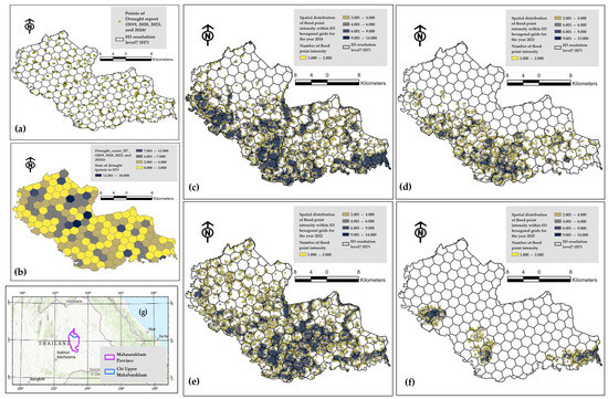
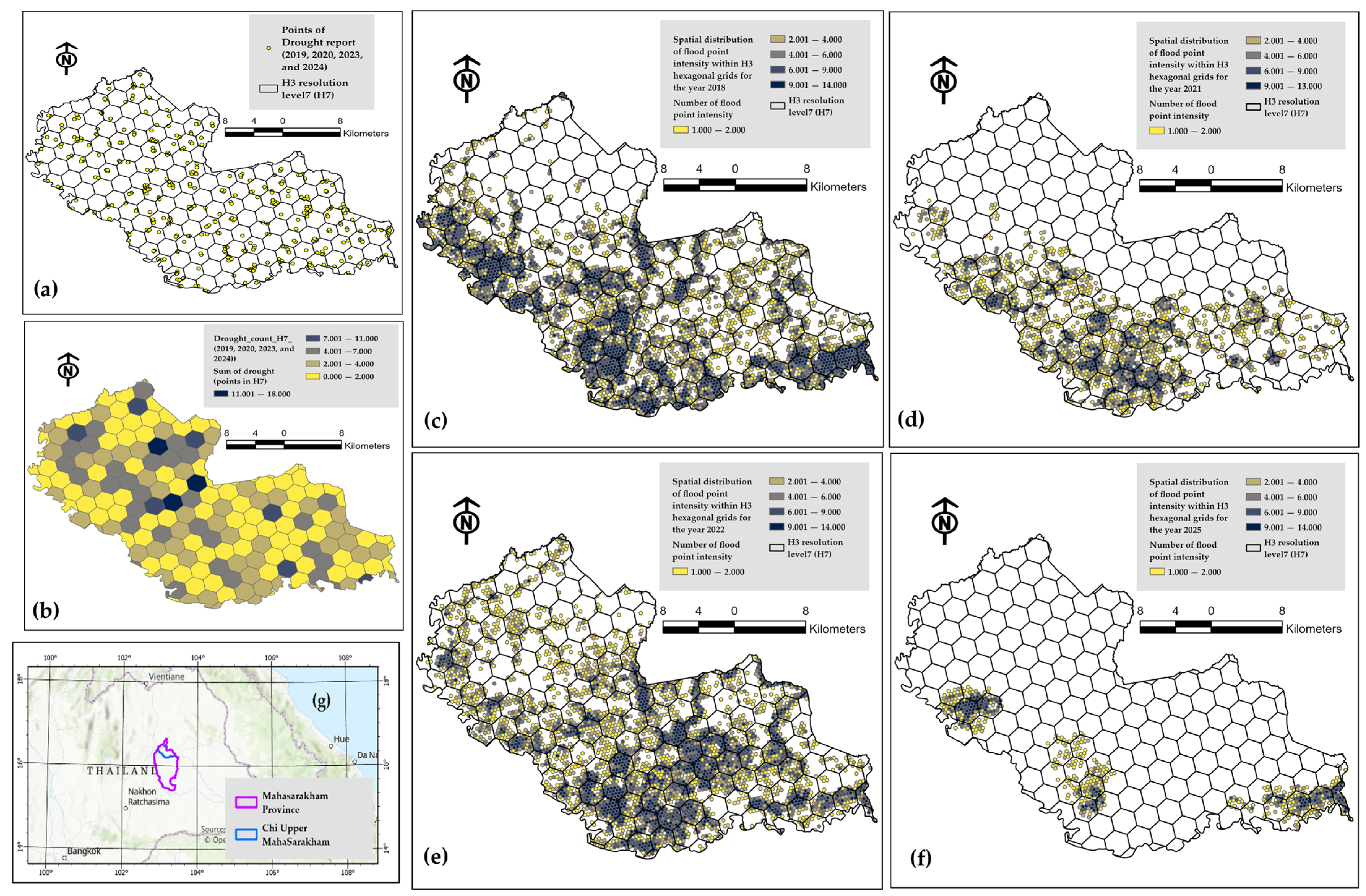
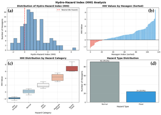
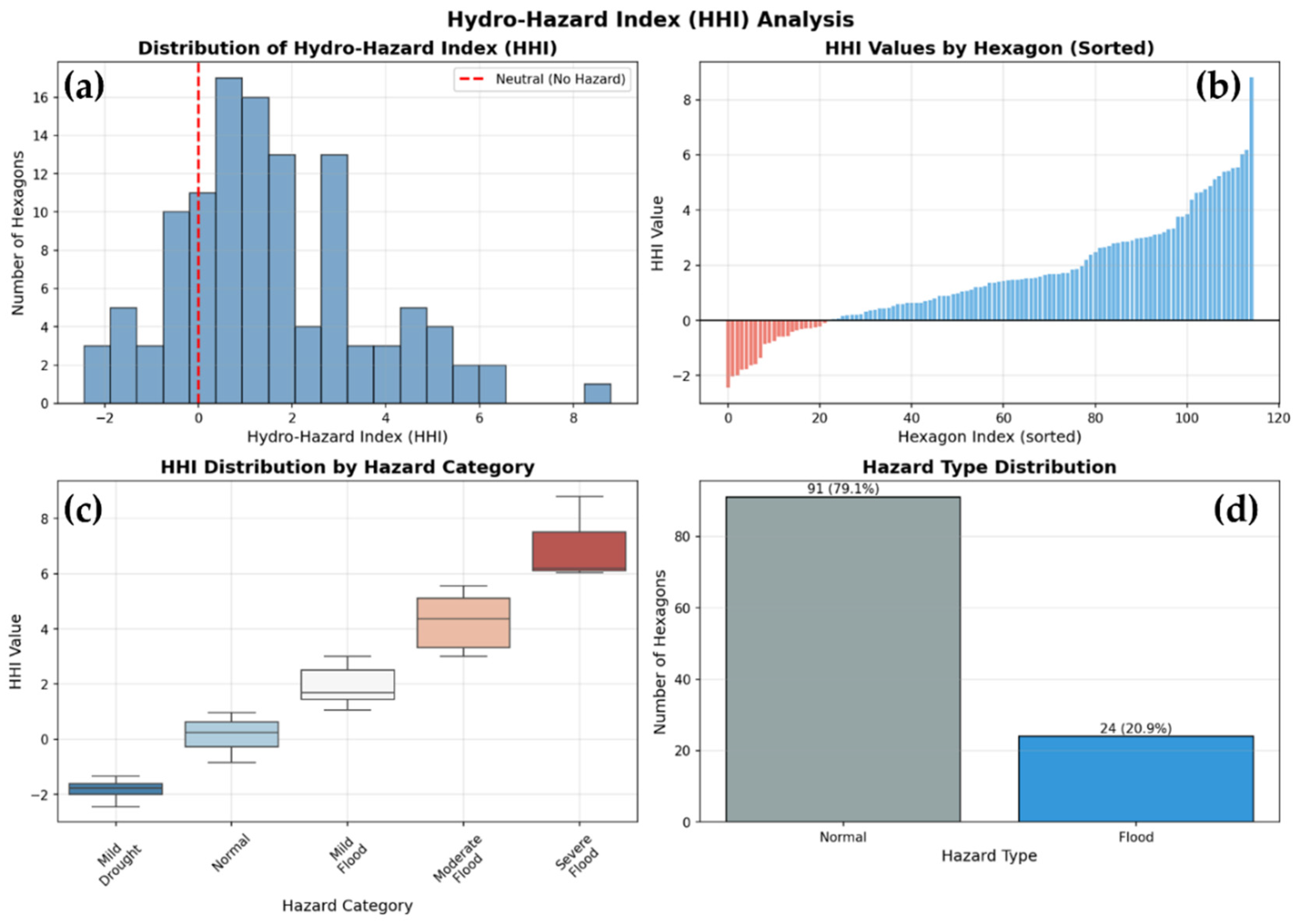
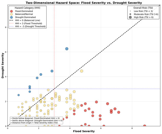
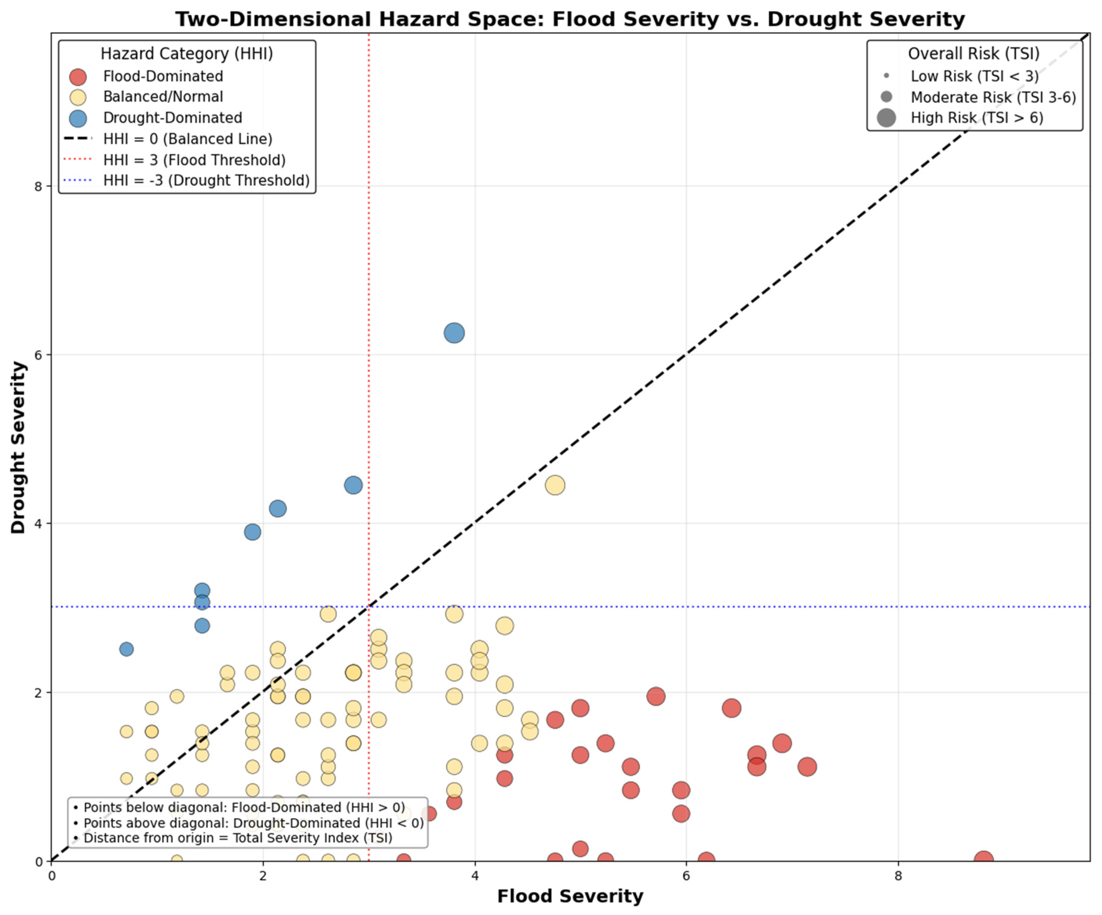
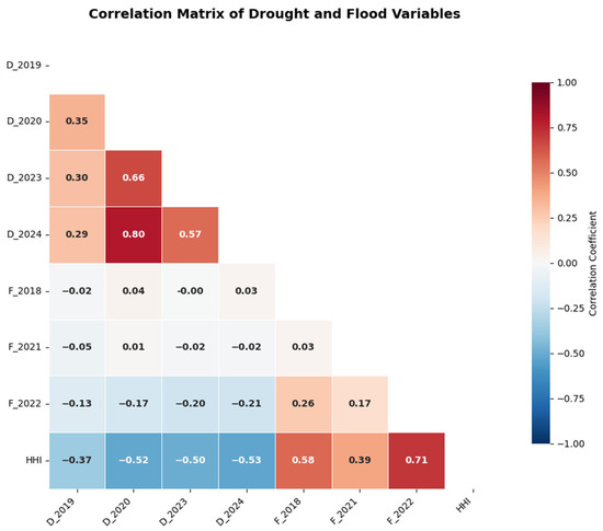
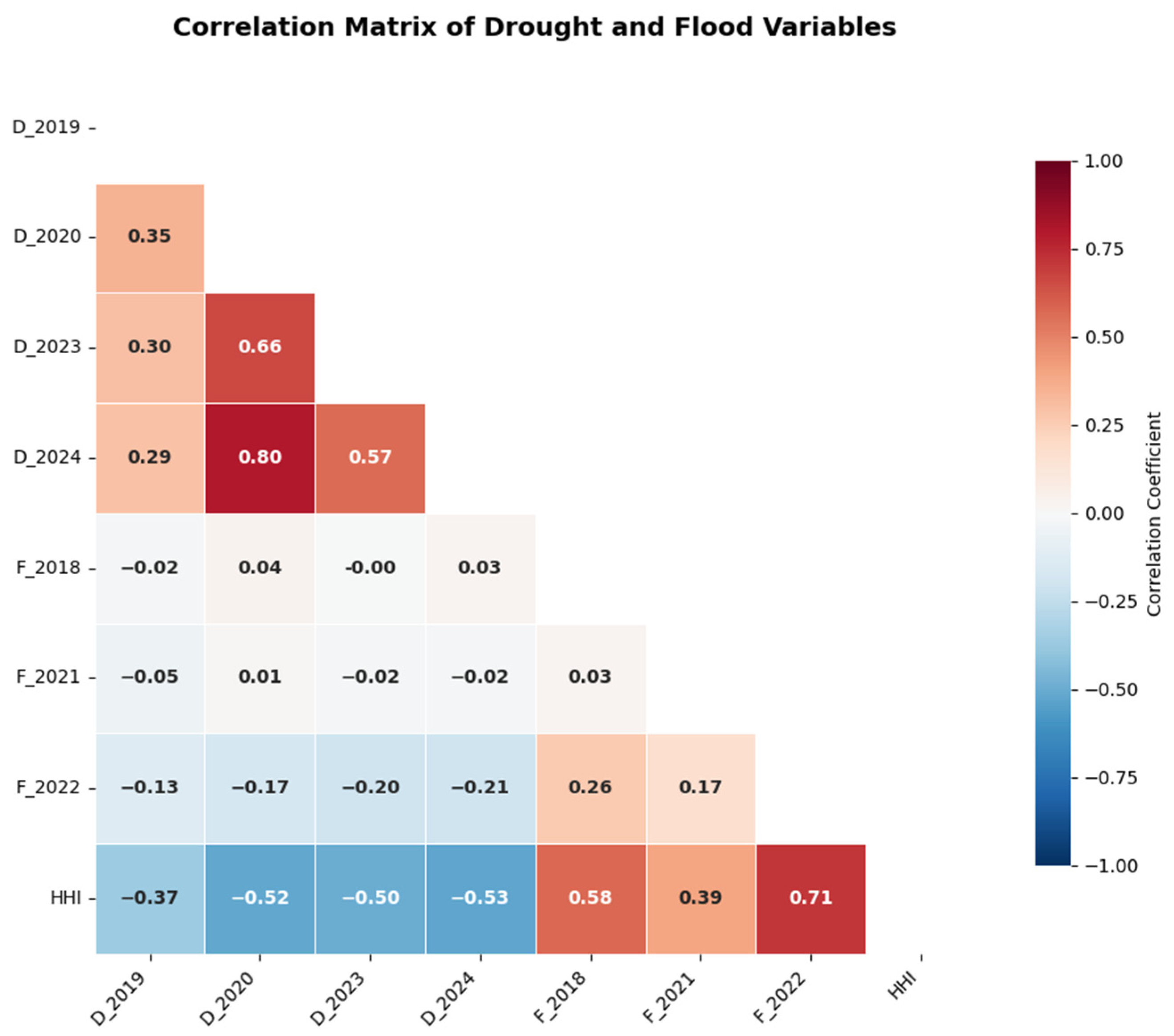
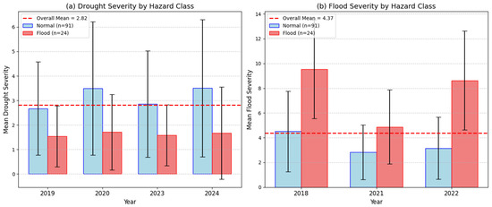
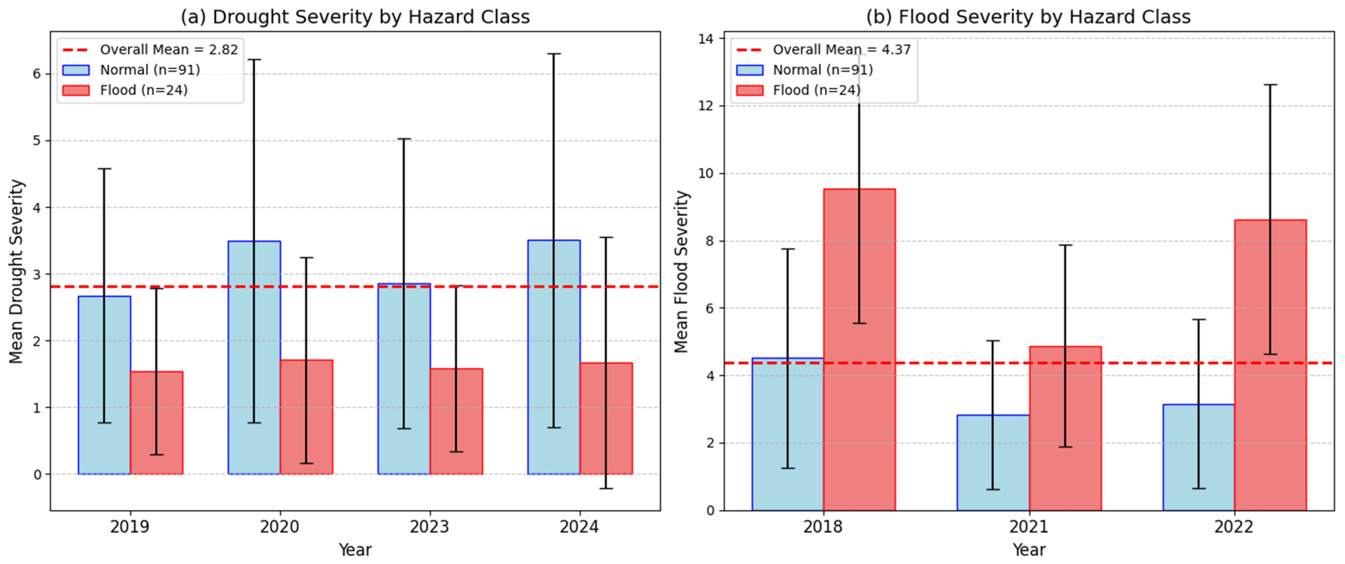
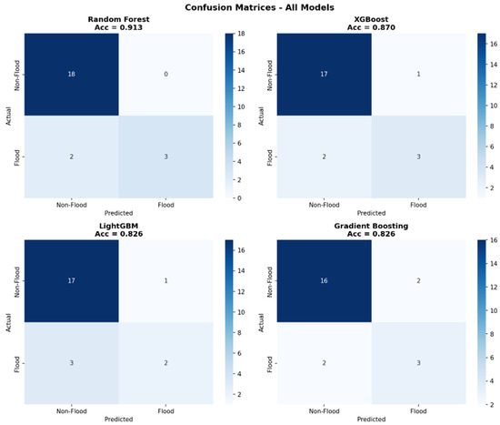
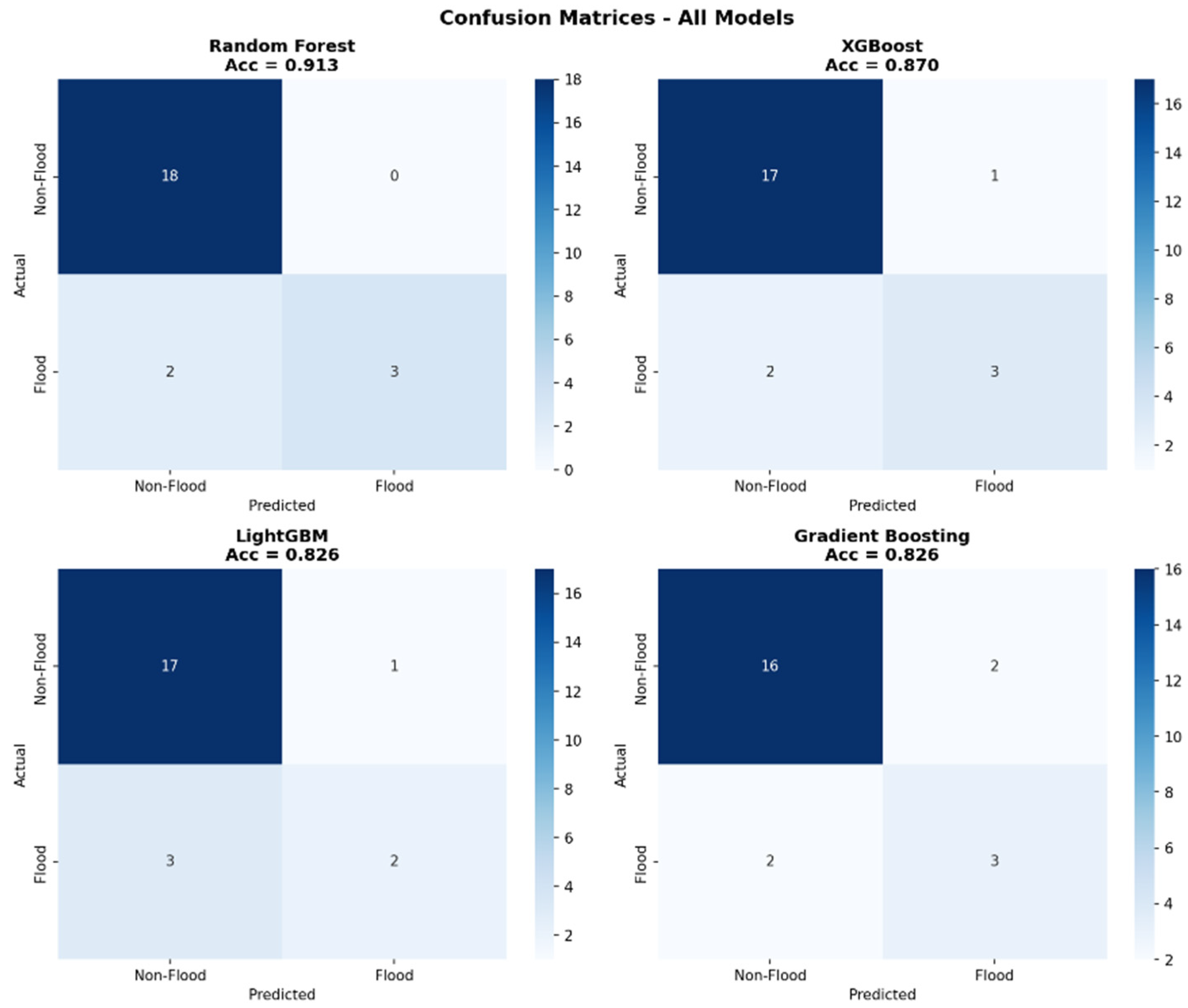
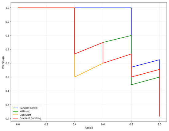
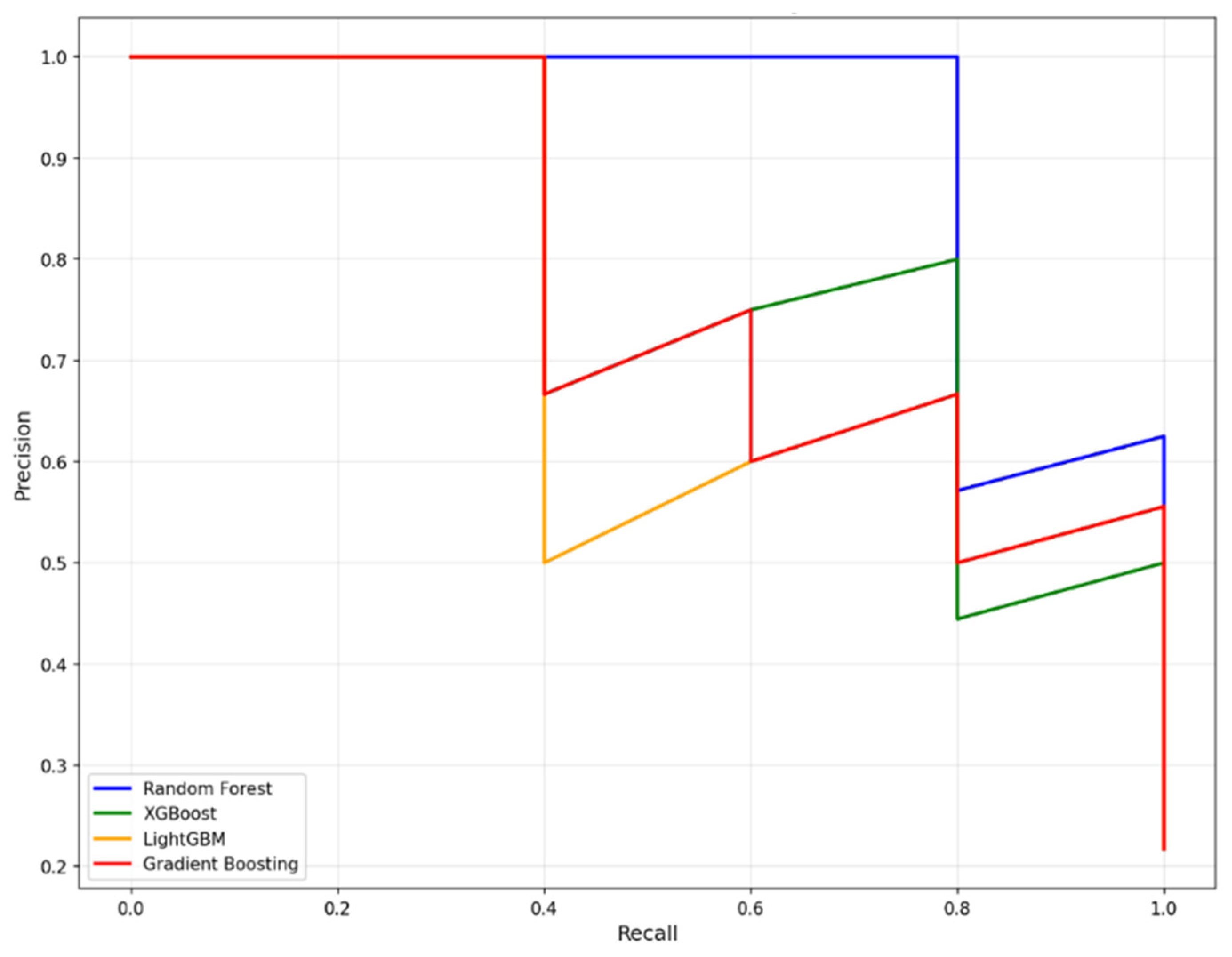
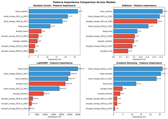
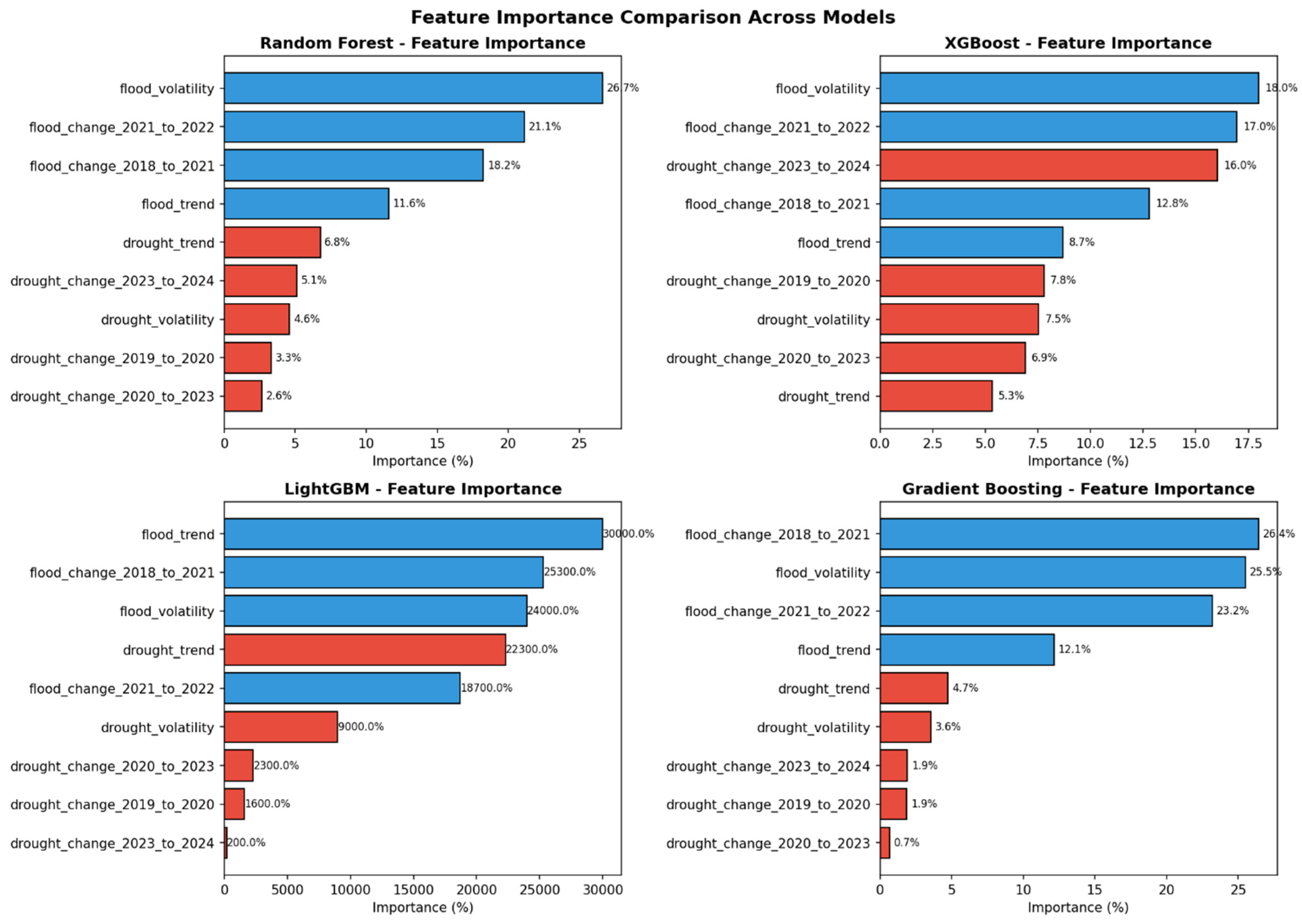
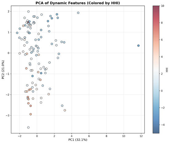
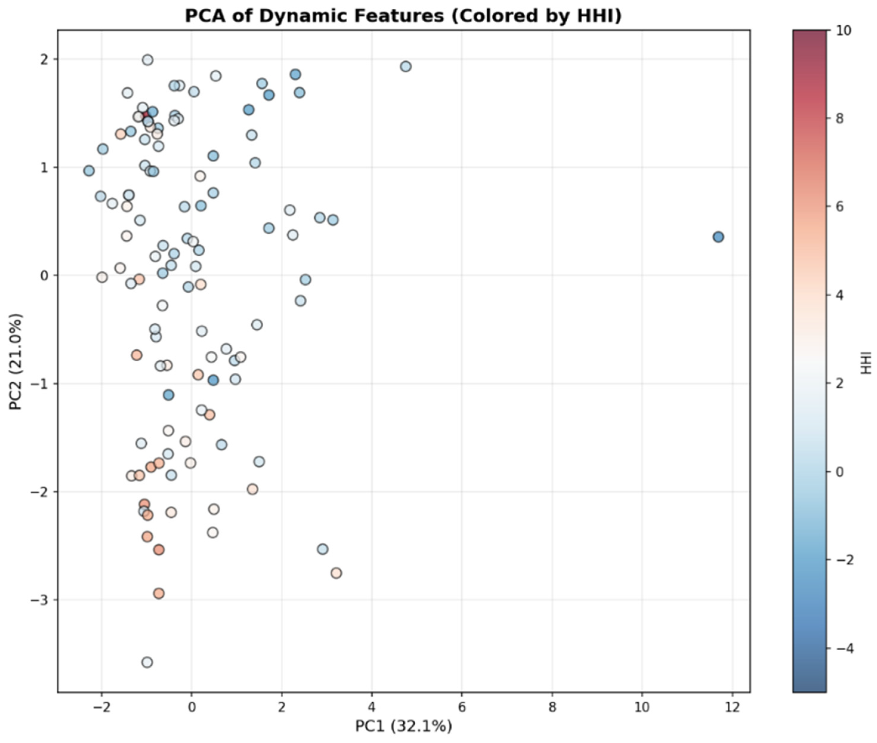
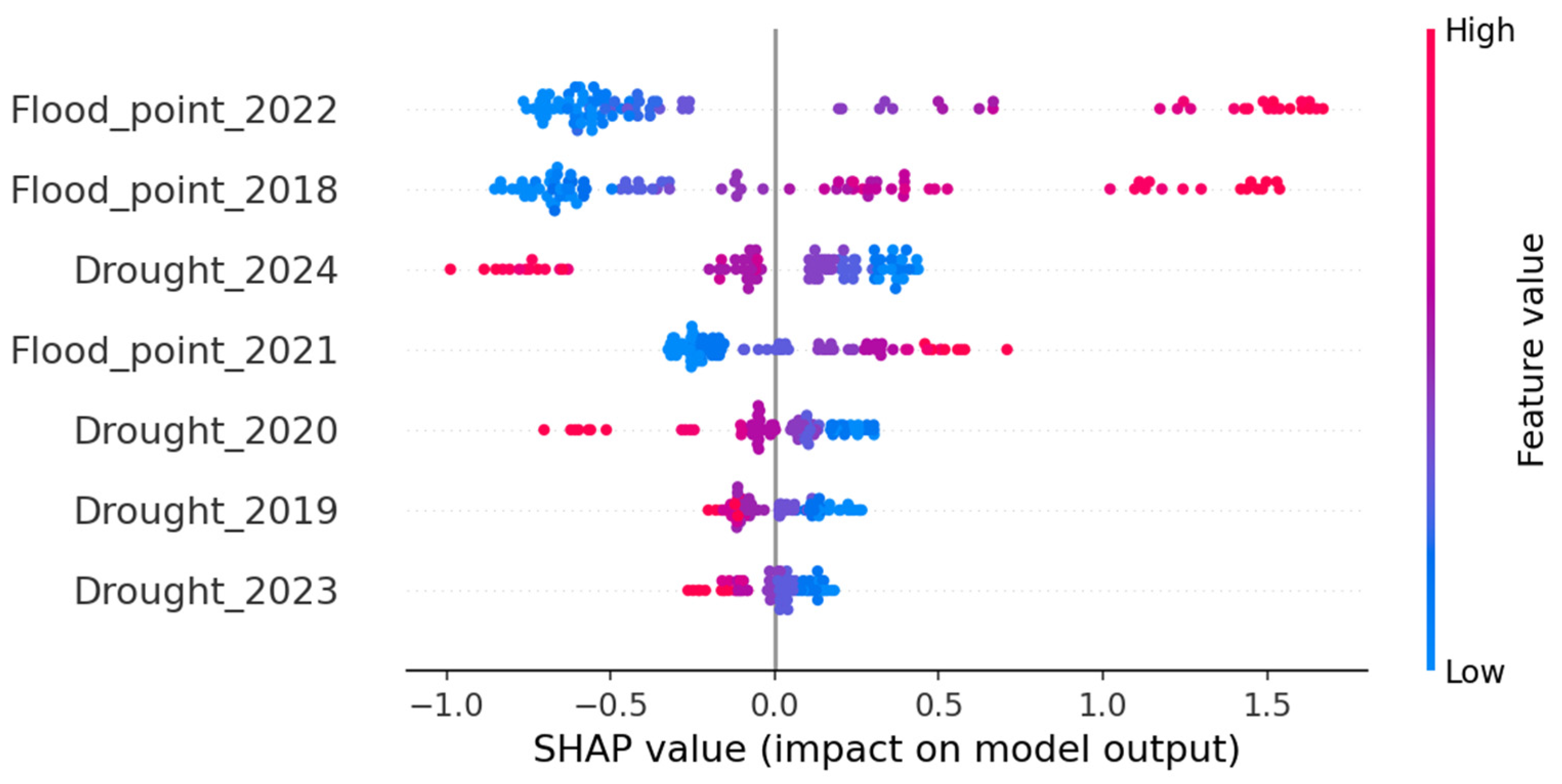
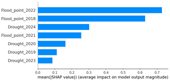
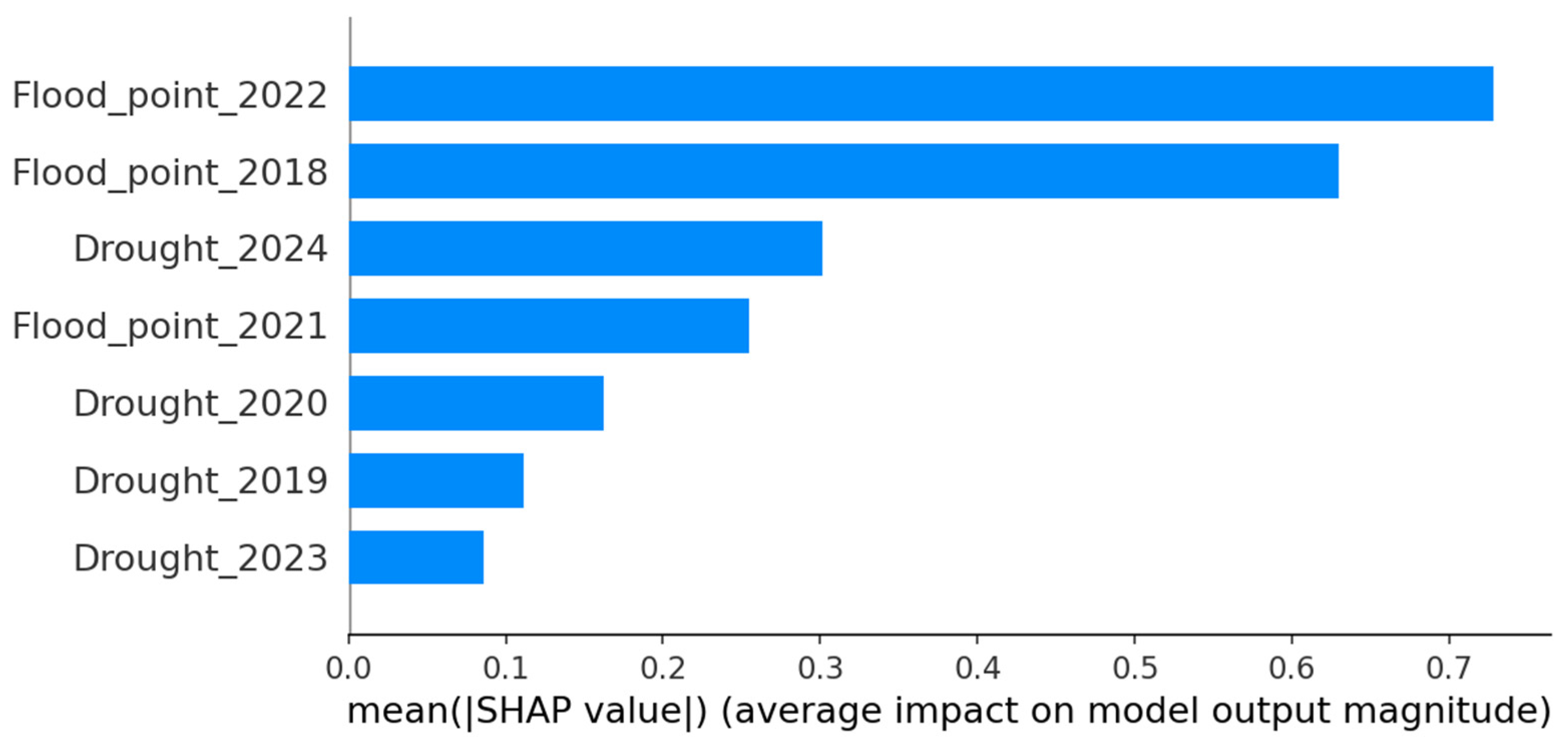
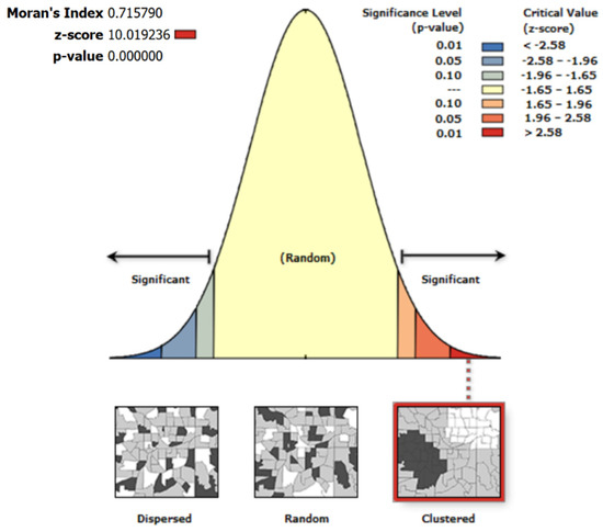
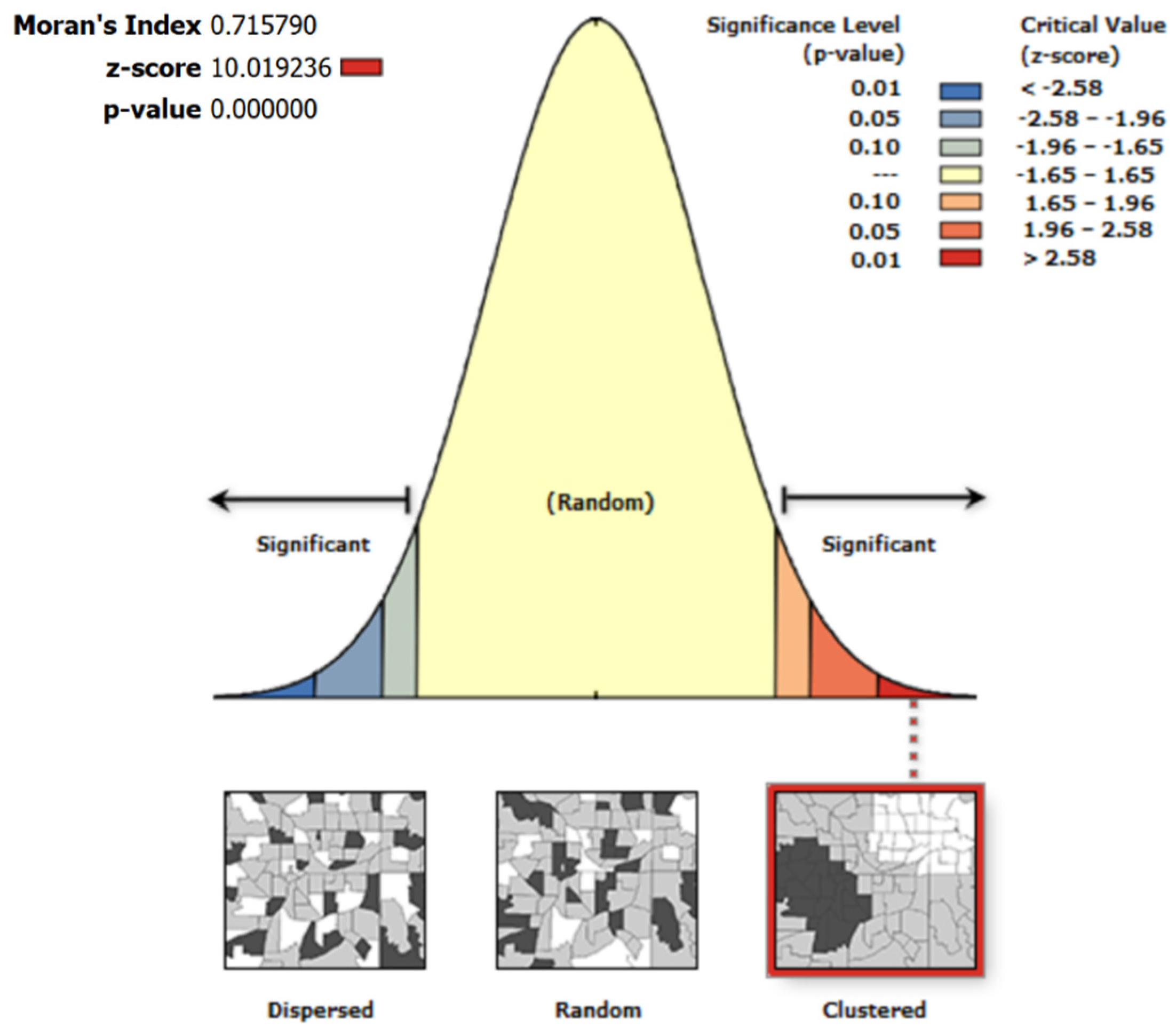

Disclaimer/Publisher’s Note: The statements, opinions and data contained in all publications are solely those of the individual author(s) and contributor(s) and not of MDPI and/or the editor(s). MDPI and/or the editor(s) disclaim responsibility for any injury to people or property resulting from any ideas, methods, instructions or products referred to in the content. |
© 2026 by the authors. Licensee MDPI, Basel, Switzerland. This article is an open access article distributed under the terms and conditions of the Creative Commons Attribution (CC BY) license.