Article

Decadal SAR Evidence of Re-Encroachment into Hazardous Floodplains Following the 2020 Relocation Policy in Beledweyne, Somalia

1
Disaster & Risk Management Laboratory, Interdisciplinary Program in Crisis & Disaster and Risk Management, Sungkyunkwan University (SKKU), Suwon 16419, Gyeonggi, Republic of Korea
2
School of Geography, Faculty of Environment, University of Leeds, Woodhouse Lane, Leeds LS2 9JT, UK
3
Geodesy Laboratory, Civil & Architectural and Environmental System Engineering, Sungkyunkwan University (SKKU), Suwon 16419, Gyeonggi, Republic of Korea
*
Authors to whom correspondence should be addressed.
Sustainability 2026, 18(14), 7060; https://doi.org/10.3390/su18147060
Submission received: 30 May 2026 / Revised: 5 July 2026 / Accepted: 9 July 2026 / Published: 10 July 2026

Abstract

Recurrent flooding along the Wabi Shabelle River has repeatedly displaced communities in Beledweyne, Somalia, prompting a 2020 government-led relocation policy intended to reduce long-term flood risk exposure. Whether such resettlement constitutes a durable change-detection method disaster risk reduction strategy in semi-arid East Africa remains empirically untested. We integrate ten years of Sentinel-1 SAR (259 scenes, 2015–2025), three global DEMs (Copernicus GLO-30, FABDEM, SRTM), CHIRPS precipitation, and BFAST changepoint analysis to map flood frequency at 10 m resolution. The Z-score showed the strongest coupling with 12-day cumulative precipitation (Pearson r = +0.338; block-bootstrap 95% CI [+0.13, +0.49], excluding zero) and strong agreement with the log-ratio method (r = +0.676), whereas the conventional fixed −17 dB threshold produced a physically implausible negative correlation (r = −0.248). These conclusions were stable across alternative thresholds. HAND from all three DEMs was positively associated with flood frequency (Spearman ρ ≈ +0.30); GLO-30 and FABDEM were near-equivalent in this low-relief setting (median pairwise difference, 0.13 m). BFAST detected 476,955 changepoints (49.9% post-2020 vs. 35.6% pre-2020), concentrated in high-flood-frequency pixels (Kolmogorov–Smirnov D = 0.854, p < 0.001). The mean flooded area fraction rose from 4.68% to 5.61%, a relative increase of +19.8% (95% CI 9.1–32.0); this remained significant after controlling for precipitation (+0.96 pp, p < 0.001) and excluding the extreme 2023 events (+0.81 pp). Because standard optical and multi-year surface water products are unsuitable for pixel-level validation in this turbid seasonal river, we demonstrate that SAR flood frequency is significantly higher within independently mapped JRC water corridors (median, 0.070 vs. 0.042; p < 0.001). These convergent lines of evidence are consistent with re-encroachment into hazardous floodplains, suggesting that structural relocation alone is unlikely to deliver durable flood risk reduction without parallel investment in tenure security, livelihoods, and inclusive governance (SDGs 11.5, 13.1). The reproducible, open-source SAR framework provides a transferable monitoring template for data-sparse Horn of Africa floodplains.

1. Introduction

Somalia’s Juba and Shabelle basins are among the most flood-prone regions in the Horn of Africa, where riverine flooding has become more frequent and severe over the past decade [1]. In 2020, the town of Beledweyne was inundated by the Shabelle River, displacing most of its population [1]; hydrodynamic modeling of the basin projects 100-year flood depths exceeding 7 m [2], and earlier observations of the 2016 flood documented disruption to tens of thousands of residents [3]. These hazards compound with broader stressors: millions of Somalis have been displaced by recurring droughts and floods since 2016 [4,5], with displacement concentrated in the inter-riverine zones where land competition amplifies vulnerability [6,7].
In response to the 2020 floods, Somali authorities initiated a relocation policy to move flood-exposed households beyond the active floodplain. Although anecdotal reports suggest substantial re-encroachment back into hazard zones, no peer-reviewed study has empirically evaluated the spatial outcome of this policy. The wider literature offers a cautionary frame: floodplain urban area nearly doubled globally between 1985 and 2015, fastest in the most hazardous zones [8], and agent-based modeling shows low-income households can become trapped in hazard areas as safer land becomes unaffordable [9]. Resettlement programs that ignore underlying vulnerabilities—land access, livelihoods, governance—have repeatedly failed in Africa [10,11,12,13]. This motivates an empirical, reproducible test of whether the Beledweyne relocation actually reduced floodplain occupancy.
Such a test requires reliable flood monitoring. Sentinel-1 SAR is well suited because of its all-weather, day–night acquisition, but the most common approach—a fixed backscatter threshold (e.g., VV < −17 dB)—performs poorly in semi-arid terrain, where dry sand, tarmac, and smooth bare soil produce low backscatter overlapping with open water [3,14,15,16,17]. Multi-temporal change detection [15,16,18,19,20], adaptive thresholding [21,22], and per-pixel statistical normalization (Z-score) and log-ratio indices [23,24,25,26,27,28,29] outperform global thresholds in heterogeneous landscapes, and reviews now favor adaptive, data-driven thresholds over single global thresholds [14,25,30]. We therefore compare a fixed threshold against Z-score and log-ratio change detection in this setting.
To check that detected inundation is terrain-consistent, we use height above nearest drainage (HAND), a DEM-derived proxy for fluvial flood susceptibility [31,32] that approximates hydrodynamic outputs at low cost [33,34,35,36,37,38,39,40] but is sensitive to DEM quality. FABDEM, a bare-earth correction of Copernicus GLO-30, is the most accurate global 30 m DEM overall [41], yet no published evaluation has assessed FABDEM-HAND performance in semi-arid East African floodplains [42]. Finally, attributing land surface change to a policy requires unsupervised breakpoint detection; we use BFAST [43,44,45,46,47], which has been widely applied to vegetation, hydrological, fire, and land policy change [48,49,50,51,52,53,54,55,56,57,58,59,60].
This study addresses three questions: (RQ1) Which SAR detection method—fixed, Z-score, or log-ratio—yields a flood frequency map most consistent with rainfall forcing and HAND-based terrain susceptibility? (RQ2) How strongly does the choice of global DEM affect HAND-based validation? (RQ3) Did the 2020 relocation produce a measurable regime shift in floodplain occupancy detectable through BFAST, with changepoints concentrated in high-frequency flood zones? We develop a fully reproducible multi-method SAR framework and, in this revision, additionally quantify estimation uncertainty, threshold sensitivity, revisit interval effects, and independent spatial consistency.

2. Materials and Methods

2.1. Study Area

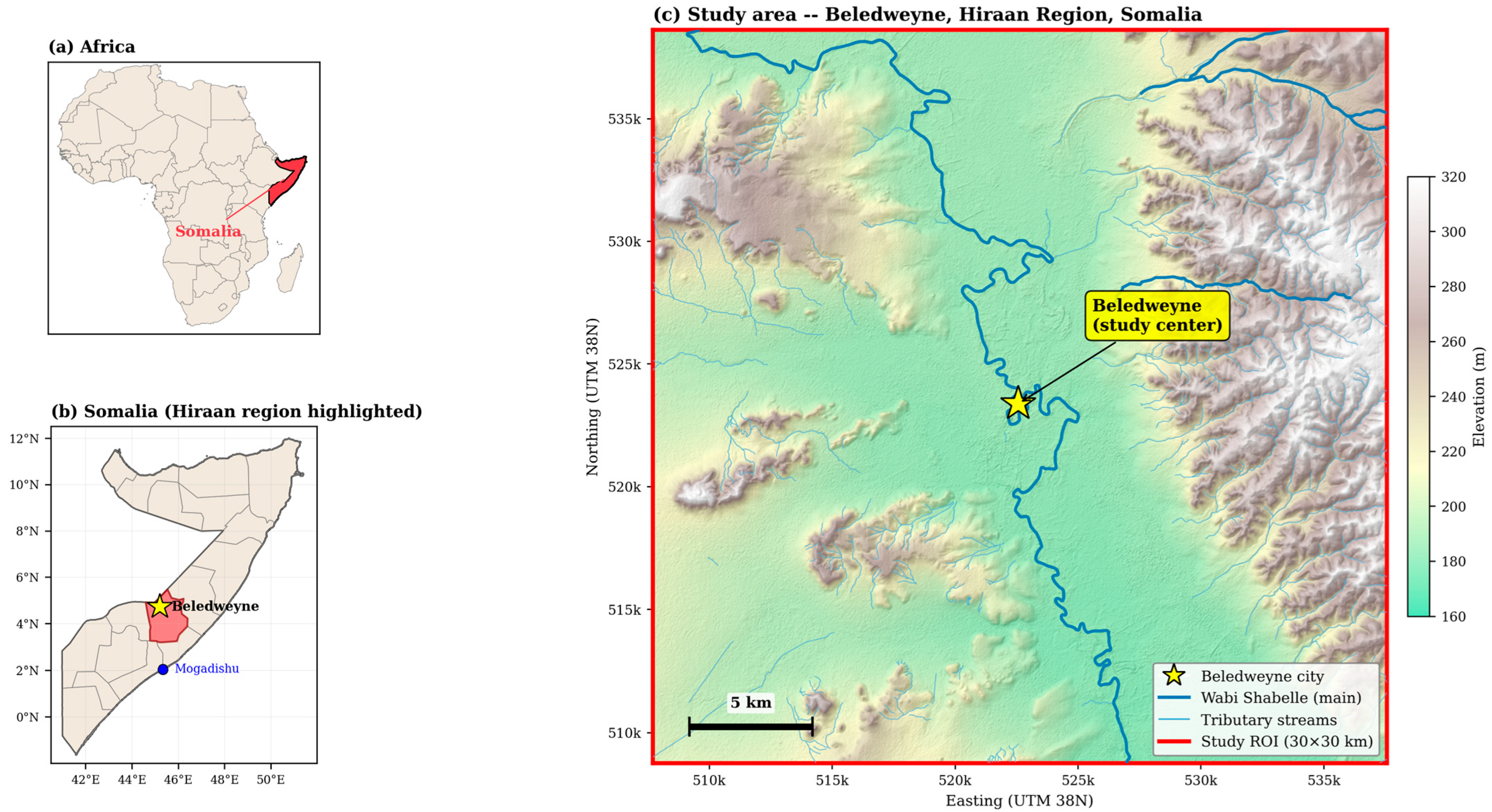
The study area covers a 30 × 30 km region (~900 km2) centered on Beledweyne, capital of Somalia’s Hiraan Region (4.60–4.87° N, 45.07–45.34° E; EPSG:32638), traversed by the Wabi Shabelle River (Figure 1). Elevation ranges from 170 to 358 m (mean 217 m), and the climate is semi-arid (Köppen BSh) with a mean annual precipitation of 278 mm yr−1 (CHIRPS 2015–2025) concentrated in two rainy seasons, Gu (April–June) and Deyr (October–December). Major flood events occurred in 2018 (Gu), 2019 (Deyr), 2020 (Gu), and 2023 (both seasons). The permanent town population is estimated at ~115,000, although flood-induced displacement causes large transient fluctuations. Study-area characteristics are summarized in Table 1.

2.2. Overall Workflow

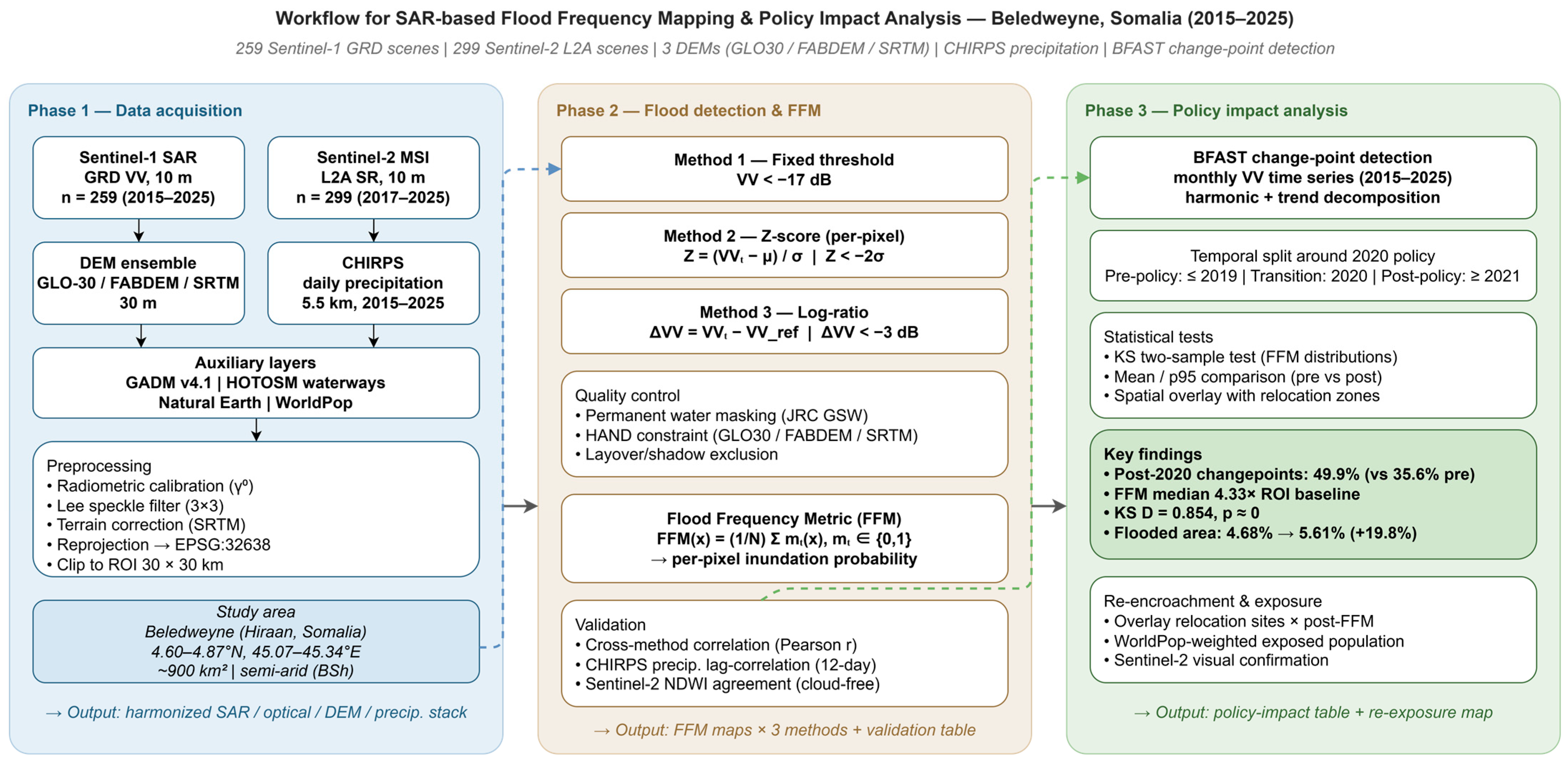
The processing chain comprises seven sequential stages: (i) acquisition of Sentinel-1 SAR, Sentinel-2 optical, DEM, CHIRPS, and ancillary GIS layers; (ii) preprocessing of SAR and optical indices; (iii) per-pixel flood masking using three competing methods; (iv) computation of the flood frequency metric (FFM); (v) HAND analysis for three DEMs; (vi) BFAST changepoint detection; and (vii) policy period statistical comparison, including the precipitation-controlled, uncertainty, sensitivity, and independent consistency analyses introduced in this revision (Figure 2).

2.3. Data Sources

All datasets are summarized in Table 2. Sentinel-1 GRD VV-polarized scenes (n = 259) covering January 2015 to December 2025 were obtained from Google Earth Engine (GEE) and resampled to 10 m on the EPSG:32638 grid. Sentinel-2 L2A surface reflectance scenes (n = 299) were obtained to evaluate their suitability as an independent optical reference for the SAR flood maps; as shown in Section 3.5, rainy-season cloud cover and high turbidity render them unsuitable for pixel-level validation in this setting. Three global 30 m DEMs were acquired (Copernicus GLO-30, FABDEM v1.2, SRTM GL1 v3). CHIRPS daily precipitation (n = 4018 days) was extracted at 5.5 km resolution. Administrative boundaries are from GADM v4.1, hydrography from HOTOSM Somalia waterways, and continental boundaries from Natural Earth; the multi-year Joint Research Centre Global Surface Water (JRC GSW) product was additionally used for independent spatial consistency checking (Section 2.9).

2.4. Sentinel-1 Preprocessing and SAR Flood Detection Methods

2.4.1. Sentinel-1 Acquisition and Preprocessing

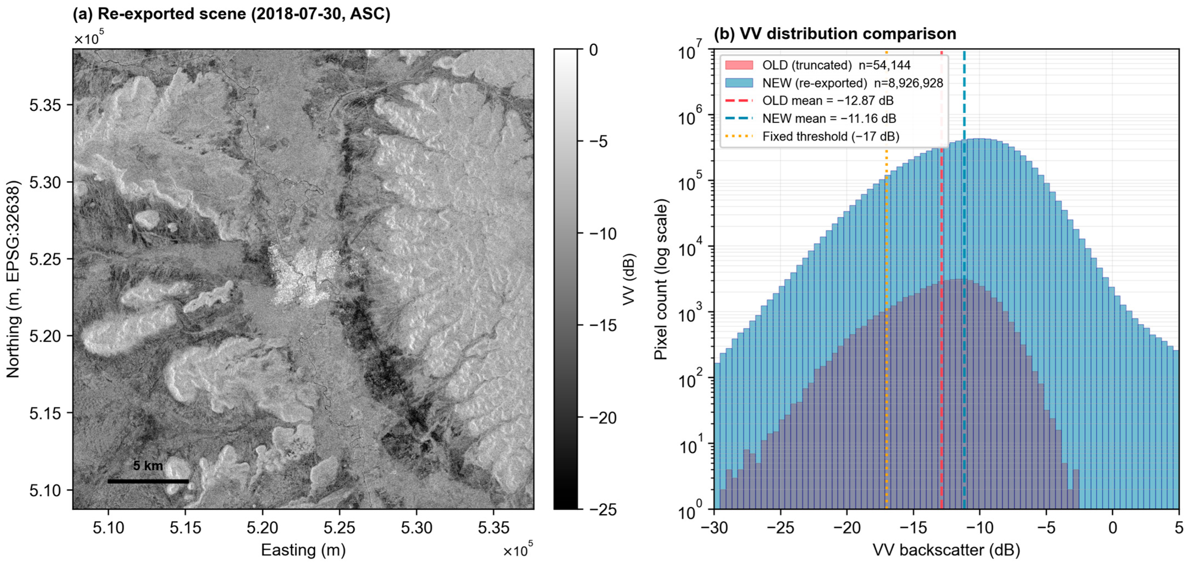
All Sentinel-1 imagery was accessed through the Google Earth Engine (GEE) COPERNICUS/S1_GRD collection, which distributes Ground Range Detected (GRD) scenes as an analysis-ready product. Prior to ingestion, GEE applies a standardized preprocessing chain to each scene using the Sentinel-1 Toolbox, comprising thermal noise removal, GRD border noise removal, radiometric calibration to the backscatter coefficient σ0, and Range–Doppler terrain correction referenced to the SRTM 30 m digital elevation model; the calibrated backscatter is provided in decibels (10·log10σ0). We filtered the collection to interferometric wide (IW) swath mode and vertical transmit/vertical receive (VV) polarization, which offers the most consistent separation between open water and land surfaces in this setting. Only descending-orbit acquisitions were retained: ascending-orbit coverage over the study area was intermittent during 2018–2020, and mixing look geometries introduces incidence-angle-dependent and orbit-dependent backscatter offsets that would confound the per-pixel change-detection statistics described below. Restricting the analysis to a single, consistent acquisition geometry therefore removes a systematic source of variability from the multi-temporal stack. The resulting 259-scene time series (2015–2025) was reprojected to EPSG:32638 (UTM Zone 38N) and resampled to a common 10 m grid to ensure exact pixel-to-pixel correspondence across all scenes, the three DEM-derived layers, and the CHIRPS precipitation series. Because the change-detection and BFAST analyses operate on relative temporal deviations at each pixel, backscatter values were not additionally speckle-filtered prior to per-pixel statistical normalization, which would otherwise attenuate the transient inundation signal the methods are designed to detect; the terrain-flattened σ0 time series from GEE was used directly. During quality-control screening, one ascending-orbit scene (30 July 2018) was found to be spatially truncated at the Google Earth Engine export stage and was replaced with a re-exported version; the residual impact of this substitution on the long-term reference composite mean was below 0.02 dB (Figure A1, Table A1). Three competing flood detection strategies were then implemented and compared on this common stack (Table 3).

2.4.2. Fixed Threshold (−17 dB)

As a baseline, pixels with VV backscatter below −17 dB were labelled as flooded. This globally calibrated threshold is the most widely adopted approach for Sentinel-1 flood mapping owing to its simplicity and computational efficiency. However, it is well documented to perform poorly in semi-arid environments, where dry sand, tarmac, salt flats, and smooth bare soils exhibit specular scattering that produces low backscatter overlapping the range of open water [3,14,15,16,17]. We retain it here as a reference against which the two change-detection methods can be evaluated rather than as a recommended operational choice.

2.4.3. Z-Score Change Detection

To adapt the detection rule to local backscatter conditions, a per-pixel dry-season reference was constructed from Jilaal (January–February) acquisitions in the pre-policy years of 2015–2019 using Welford’s online algorithm, yielding the pixel-wise mean (μ) and standard deviation (σ) of VV backscatter while requiring only a single pass through the stack. Pixels with negligible temporal variability (σ < 0.1 dB) or with a majority of missing observations were masked to avoid unstable normalization. For every subsequent scene, a standardized anomaly Z = (VV − μ)/σ was computed, and pixels with Z < −2σ—that is, a backscatter drop significantly below the local dry-season baseline—were labelled as flooded. Restricting the reference to dry-season, pre-policy acquisitions is a deliberate design choice: it prevents the flood and post-policy signals that the method is intended to detect from contaminating the baseline against which change is measured. Because the normalization is performed independently at each pixel, the method automatically accommodates the strong spatial heterogeneity in background backscatter that characterizes semi-arid floodplains and is therefore expected to outperform a single global threshold [23,24,25].

2.4.4. Log-Ratio Change Detection

As an independent change-based comparator that does not rely on the temporal variance, a log-ratio index was computed for each scene relative to the same dry-season reference mean (ΔVV = VV_scene − μ, in decibels, where a difference in the dB domain is equivalent to the logarithm of the linear backscatter ratio). Pixels with ΔVV < −3 dB were labelled as flooded [28]. Because the Z-score and log-ratio methods respond to backscatter reduction through different formulations—normalized by local variance versus absolute magnitude, respectively—their agreement provides an internal consistency check on the detected inundation signal, whereas divergence from the fixed-threshold method helps to isolate spurious low-backscatter land surfaces.

2.4.5. Flood Frequency Metric (FFM)

For each detection method, a flood frequency metric (FFM) raster was derived as the per-pixel proportion of valid observations classified as flooded over the full 2015–2025 time series (range 0–1). Missing or masked observations were excluded from both the numerator and the denominator on a per-pixel basis so that the FFM represents the empirical inundation frequency conditional on valid acquisition rather than being biased by uneven temporal sampling. The FFM constitutes the primary spatial layer used in all subsequent HAND, changepoint, and policy period analyses.

2.5. HAND Analysis

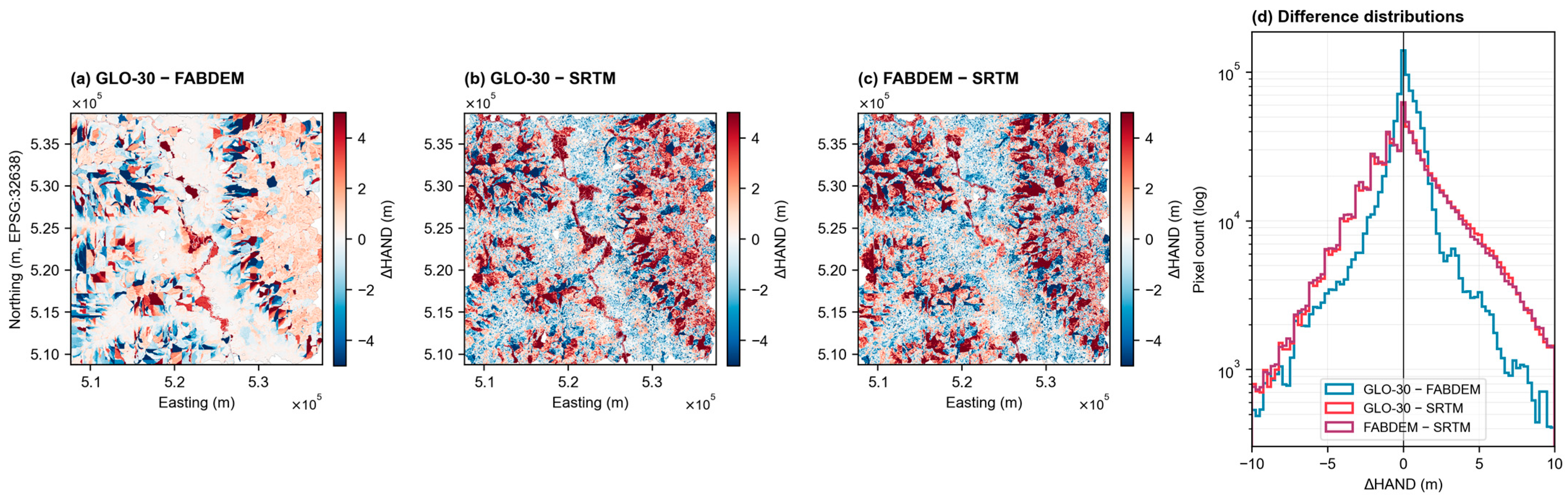
For each DEM, HAND was computed with pysheds (v0.5): (i) fill pits, (ii) fill depressions, (iii) resolve flats, (iv) D8 flow direction, (v) flow accumulation, and (vi) HAND referenced to the nearest drainage cell, with drainage defined as accumulation > 1000 cells (~0.9 km2) [31,32,37,39]. FFM was reprojected to each native 30 m HAND grid (average resampling) for comparison. To quantify DEM equivalence directly, pairwise HAND difference maps and summary statistics (mean, median, MAE, RMSE, fraction within 1 m) were computed for GLO-30, FABDEM, and SRTM (Appendix A, Figure A2).

2.6. BFAST Changepoint Detection

Monthly Sentinel-1 VV composites were stacked per pixel (2015–2025), and breakpoint detection was applied to identify the first statistically significant trend break per pixel within high-flood-frequency pixels (FFM > 0.05). The first breakpoint date was retained for spatial analysis. Pre-policy (2015–2019), 2020-transition, and post-policy (2021–2025) breakpoint counts were tabulated, and the FFM distribution at changepoint pixels was compared against the regional distribution using the Kolmogorov–Smirnov (KS) two-sample test [47]. We note that flood events themselves can generate breakpoints; the policy interpretation therefore rests not on breakpoint timing alone but on the joint concentration of post-2020 breakpoints in high-FFM pixels and on the precipitation-controlled exposure analysis (Section 2.7).

2.7. Precipitation Coupling and Policy Period Comparison

For each Sentinel-1 acquisition date, cumulative CHIRPS precipitation over the preceding 12 days was computed. Pearson and Spearman correlations between flooded area fraction (per method) and 12-day precipitation assessed physical plausibility. To separate the policy signal from hydroclimatic variability (a central concern for any pre/post comparison), we fitted ordinary least squares models with a post-policy indicator and precipitation as a covariate:
(A) flood% ~ post; (B) flood% ~ post + precip12; (C) flood% ~ post × precip12.
The 2020 transition year was excluded. We additionally re-estimated model B after removing the extreme 2023 events, compared pre/post means within matched precipitation classes, and report a precipitation-normalized flood ratio. Because Sentinel-1 revisits are not strictly regular, we characterized the revisit interval distribution, checked for seasonal sampling bias (wet vs. dry observation counts), and estimated the precipitation–flood correlation with a block bootstrap (block length = 6 acquisitions) that preserves temporal autocorrelation.

2.8. Uncertainty and Threshold Sensitivity

To quantify the uncertainty of the flooded area estimates that underlie the policy comparison, we (i) bootstrapped (10,000 resamples) the pre- and post-policy mean flooded fractions and their relative change to obtain 95% confidence intervals and (ii) repeated the entire pre/post comparison and precipitation coupling analysis across a range of detection thresholds (Z = −1.5, −2.0, −2.5σ; log-ratio = −2, −3, −4 dB) to test whether the principal conclusions are robust to the (necessarily discretionary) threshold choice.

2.9. Independent Spatial Consistency

Direct pixel-level validation against optical water masks is problematic in this setting: cloud cover during the rainy seasons and high suspended sediment loads suppress Sentinel-2 NDWI even during major floods, and the change-based SAR signal and the instantaneous optical water signal are conceptually distinct. We confirmed this empirically (Section 3.5). Multi-year surface water products are similarly limited because the Wabi Shabelle here is a seasonal river with almost no permanently inundated pixels. We therefore assess independent spatial consistency rather than pixel-level accuracy: SAR flood frequency was compared inside versus outside the JRC GSW water corridor (pixels ever observed as water) using the Mann–Whitney U test and against a high-resolution optical interpretation of the two largest flood events (Appendix A).

3. Results

3.1. Comparison of SAR Flood Detection Methods

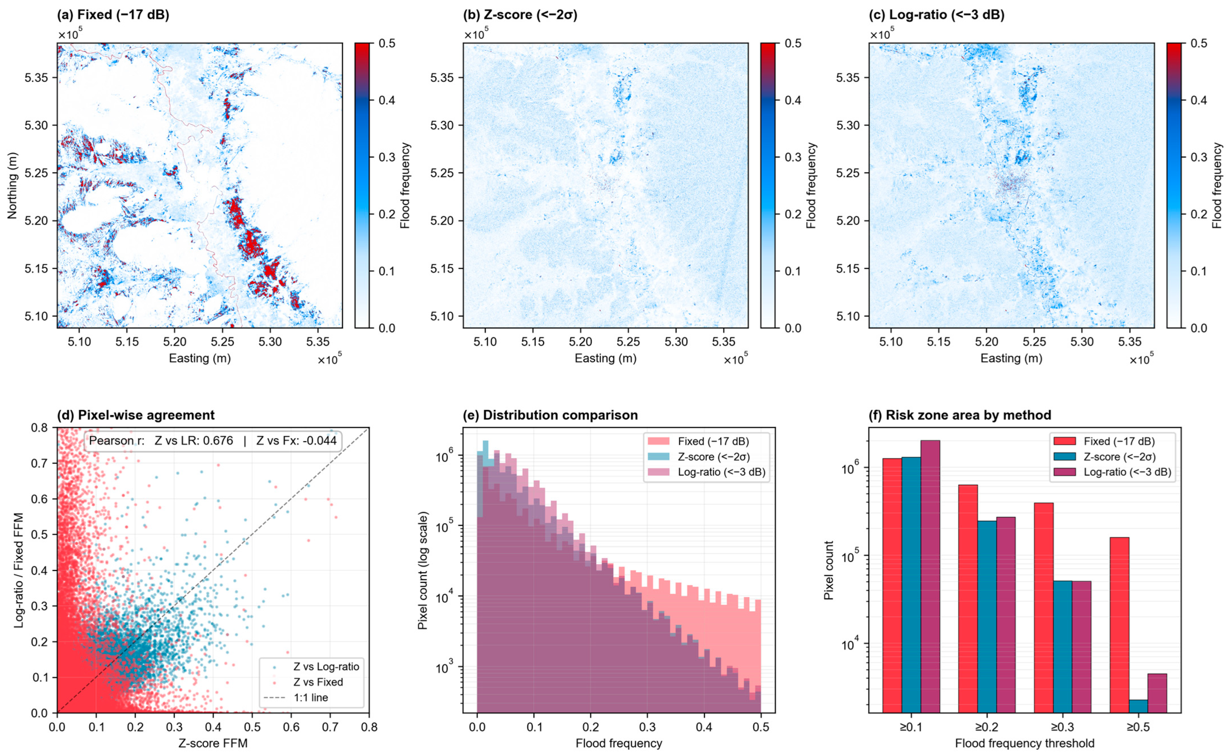
The three methods produced markedly different flood frequency maps (Figure 3). All converged on the main Wabi Shabelle channel but diverged substantially over the surrounding semi-arid lowlands. The Z-score method yielded a median FFM of 0.035 (95th percentile 0.162), the log-ratio method yielded higher values (median 0.061, p95 0.210), and the fixed-threshold method yielded an intermediate distribution (median 0.048, p95 0.192) with a distinct spatial pattern dominated by persistent dark areas inconsistent with hydrology (Table 3).
Pixel-wise analysis revealed strong agreement between Z-score and log-ratio FFM (Pearson r = +0.676) but virtually none between Z-score and fixed-threshold FFM (r = −0.044), consistent with the fixed-threshold method’s misidentification of dry-sand and smooth man-made surfaces as floodwater. The strongest evidence against the fixed threshold came from precipitation coupling: the 12-day cumulative CHIRPS precipitation correlated positively with the Z-score (r = +0.338, ρ = +0.295) and log-ratio (r = +0.209) flooded area fractions but negatively with the fixed-threshold method (r = −0.248, ρ = −0.309). This counter-intuitive negative correlation is physically implausible for a true flood signal and confirms that the −17 dB threshold is unsuitable here. The block-bootstrap 95% confidence interval for the Z-score precipitation correlation was [+0.13, +0.49], excluding zero, indicating that the coupling is robust to temporal autocorrelation and the irregular Sentinel-1 revisit interval (Section 3.4).

3.2. HAND Analysis Across Three DEMs

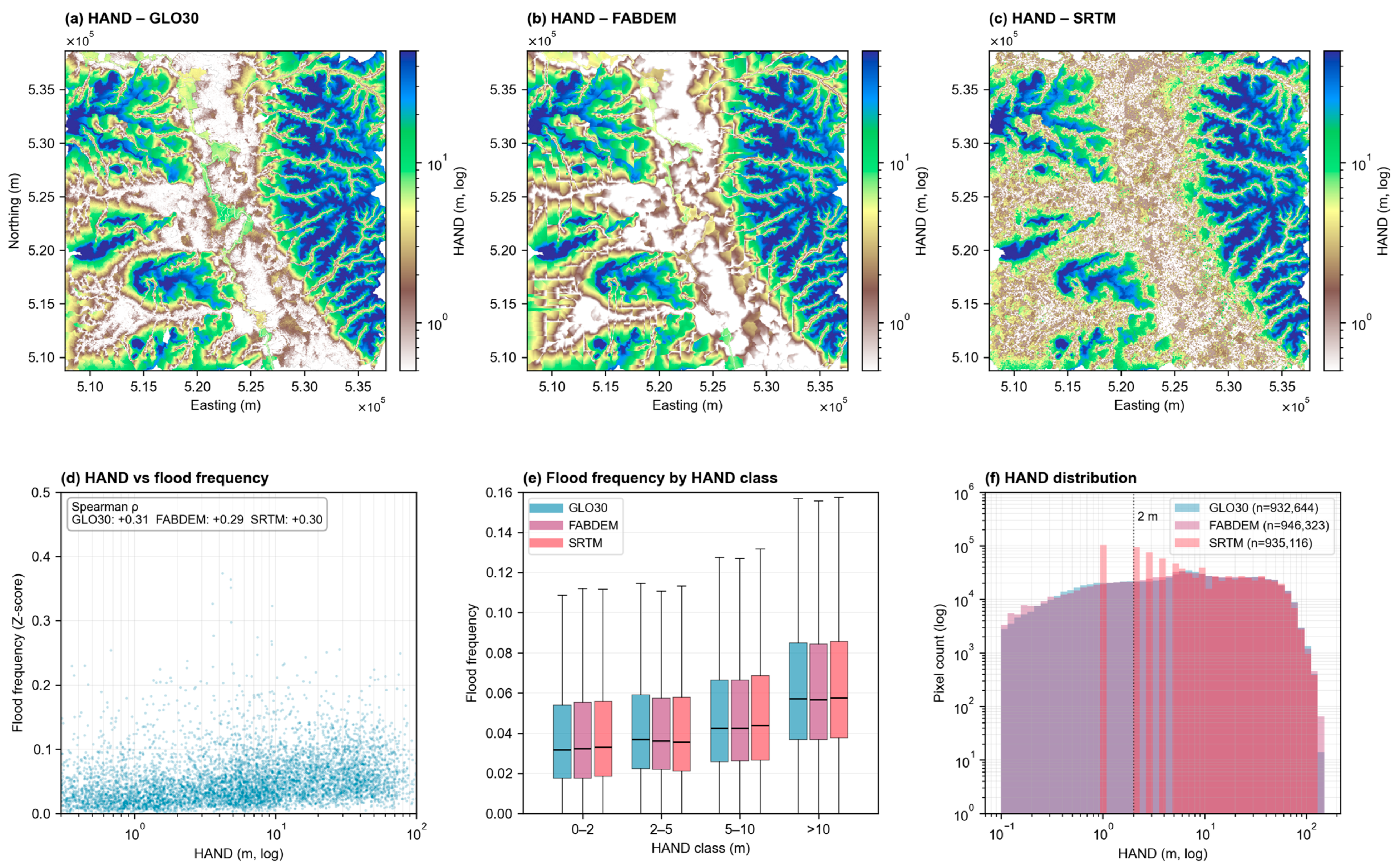
HAND maps from the three DEMs (Figure 4a–c) showed broadly consistent patterns, with HAND medians of 4.92 m (GLO-30), 4.79 m (FABDEM), and 4.99 m (SRTM). The maximum pit-filling correction differed substantially (3.51 m GLO-30, 9.77 m FABDEM, 32.0 m SRTM), reflecting SRTM’s documented noise. Pairwise difference analysis confirmed that GLO-30 and FABDEM are near-equivalent in this low-relief setting: their median HAND difference was 0.13 m (mean 0.04 m), with 59.0% of pixels within 1 m, whereas SRTM-based pairs differed more (RMSE 4.4–4.5 m; only ~33% within 1 m), consistent with SRTM noise (Appendix A, Figure A2, Table A2).
The Spearman correlation between HAND and FFM was positive and similar across DEMs (ρ = +0.31 GLO-30, +0.29 FABDEM, +0.30 SRTM; Figure 4d). Examining flood frequency by HAND class (Figure 4e) showed that mean FFM increased monotonically with HAND (0.042 at 0–2 m to 0.066 at >10 m). This positive association reflects the structure of the setting rather than a HAND failure: the permanent channel (very low HAND) is treated as temporally unchanged by the Z-score detector and therefore registers low flood frequency, while transient inundation concentrates across the surrounding low-relief floodplain. HAND thus indexes fluvial proximity but is, as expected, a non-monotonic proxy for inundation occurrence in semi-arid floodplains where overland flow paths also govern flooding [38,39,40]. The convergence of all three DEMs nonetheless supports HAND as a defensible, terrain-aware susceptibility layer in this context.

3.3. BFAST Changepoint Detection and Policy Impact

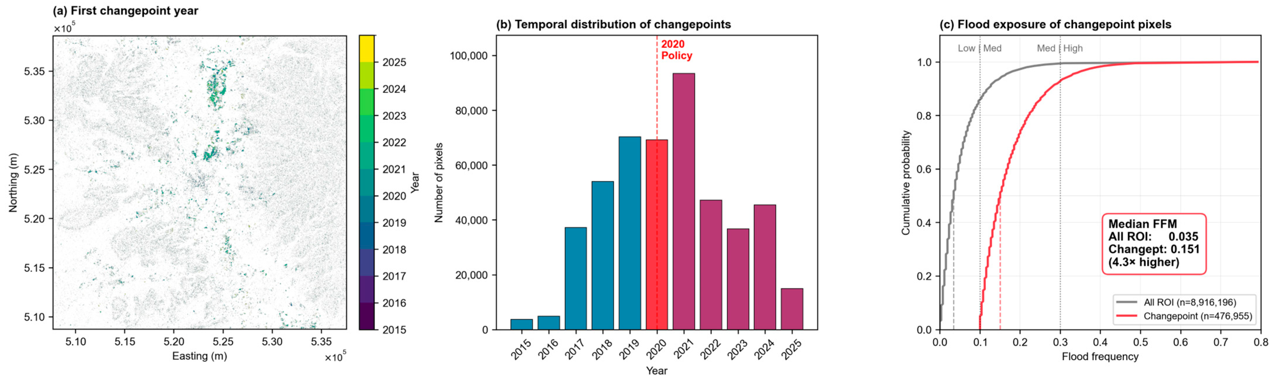
BFAST identified 476,955 valid changepoint pixels (Figure 5a). The temporal distribution (Figure 5b) showed 35.6% of breakpoints before 2020, 14.5% in 2020, and 49.9% after 2020—a +14.3 percentage-point increase in post-2020 activity relative to the pre-2020 baseline. Critically, changepoint pixels were strongly biased toward high-flood-frequency areas: the FFM median at changepoint pixels (0.151) was 4.33× the regional median (0.035), and the 95th percentile (0.328) was 2.02× the regional value (0.162). The KS two-sample test confirmed that the FFM distribution at changepoint pixels was distinct from the regional distribution (D = 0.854, p < 0.001; Figure 5c).
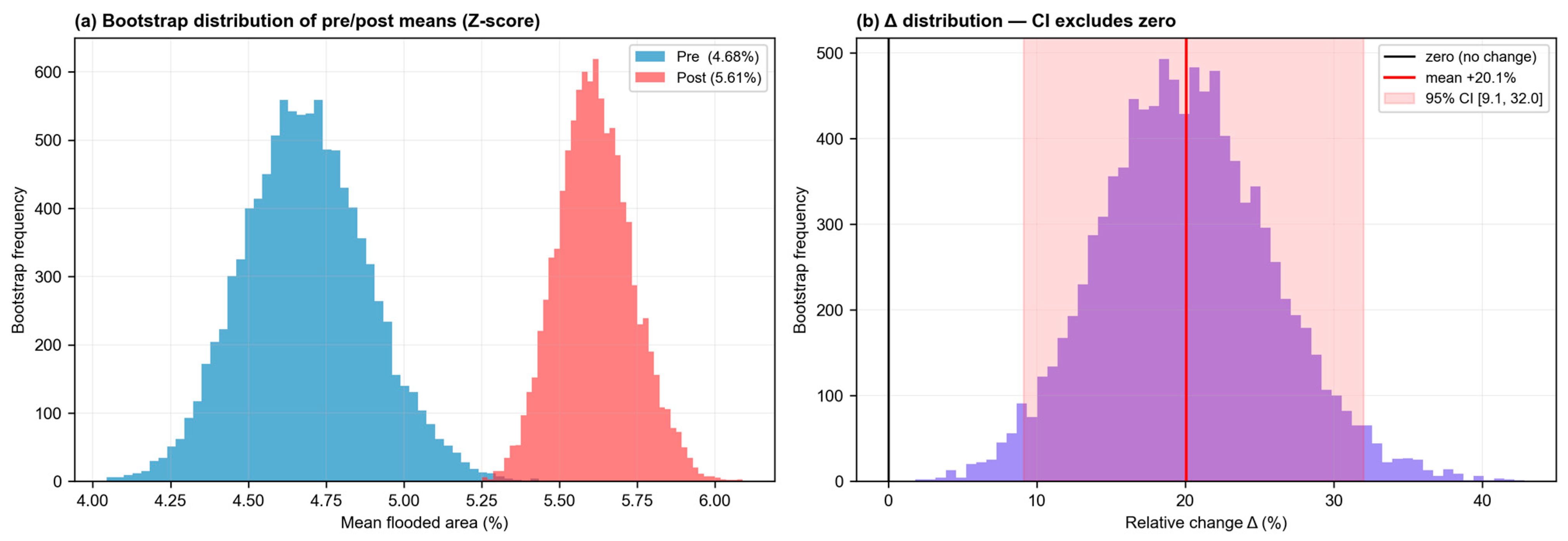
Mean flooded area fraction (Z-score) rose from 4.68% in the pre-policy period (≤2019; 95% CI 4.30–5.10) to 5.61% in the post-policy period (≥2021; 95% CI 5.39–5.87), a relative increase of +19.8% (95% CI 9.1–32.0); the confidence interval excludes zero (Figure A5). The log-ratio method showed a smaller but also significant increase (+8.6%, CI 1.2–16.2), whereas the physically implausible fixed-threshold method showed an apparent −14.1% decrease, again consistent with its misdetection of land surfaces (Table 4).

3.4. Precipitation Control and Robustness of the Policy Signal

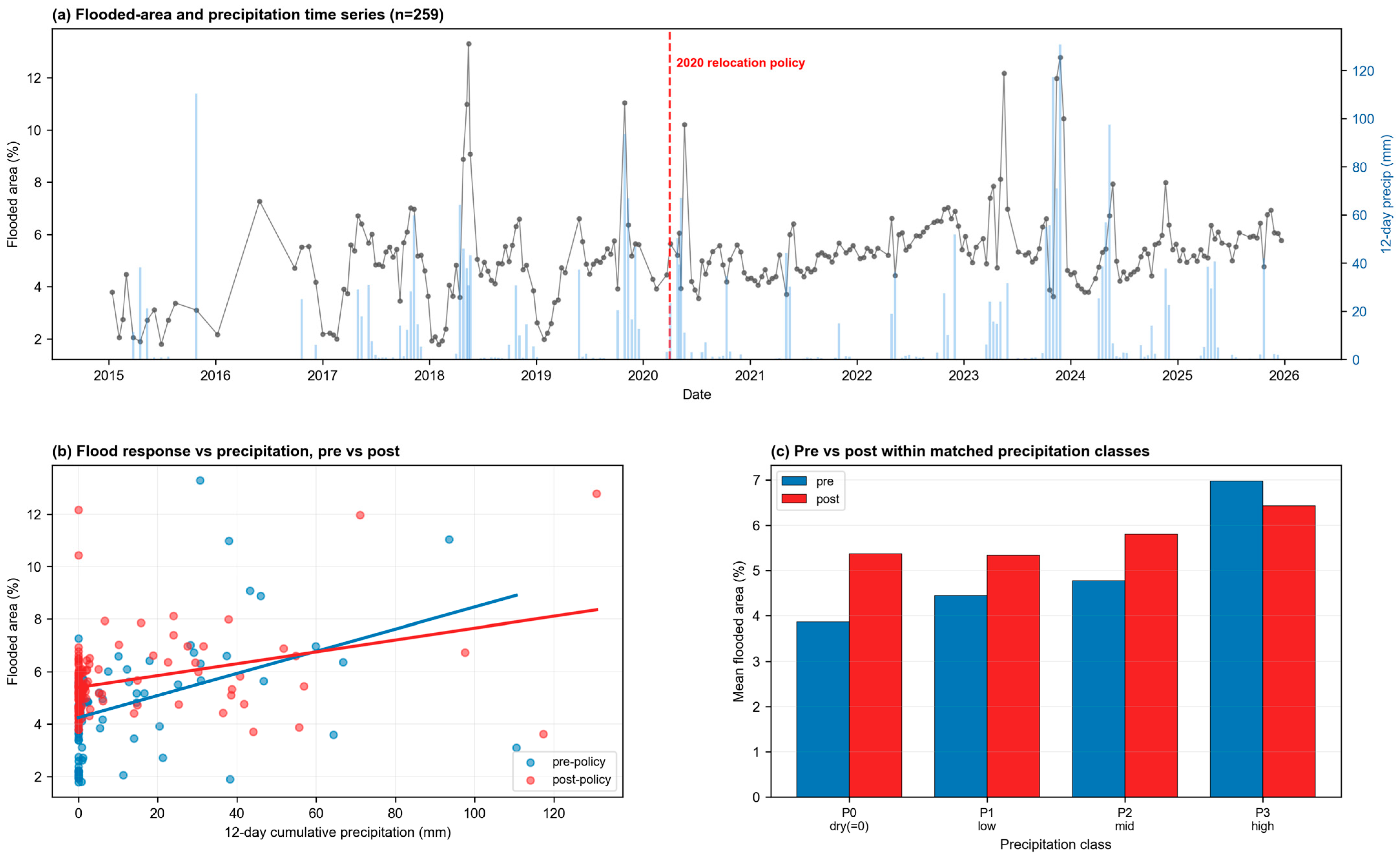
Because the post-policy increase could, in principle, reflect hydroclimatic variability rather than changed floodplain occupancy, we controlled for precipitation directly (Figure 6). With 12-day precipitation as a covariate, the post-policy indicator remained positive and highly significant (coefficient +0.96 pp, p < 0.001; adjusted R2 0.19); removing the extreme 2023 events left the effect essentially unchanged (+0.81 pp, p < 0.001). Within matched precipitation classes, post-policy flooded fractions exceeded pre-policy values in three of four classes, with the only reversal in the highest-precipitation class—consistent with saturation of the flood response during extreme rainfall, where the policy signal is necessarily masked. Thus the post-policy increase is most pronounced under ordinary low-to-moderate rainfall and is not an artefact of the 2023 events.
Sentinel-1 revisits had a median interval of 12 days, with 94.6% of intervals ≤36 days; observations were balanced between wet (n = 130) and dry (n = 129) seasons, indicating no seasonal sampling bias that could spuriously inflate the precipitation correlation. The autocorrelation-aware block-bootstrap CI for that correlation excluded zero (Section 3.1; Table A3).
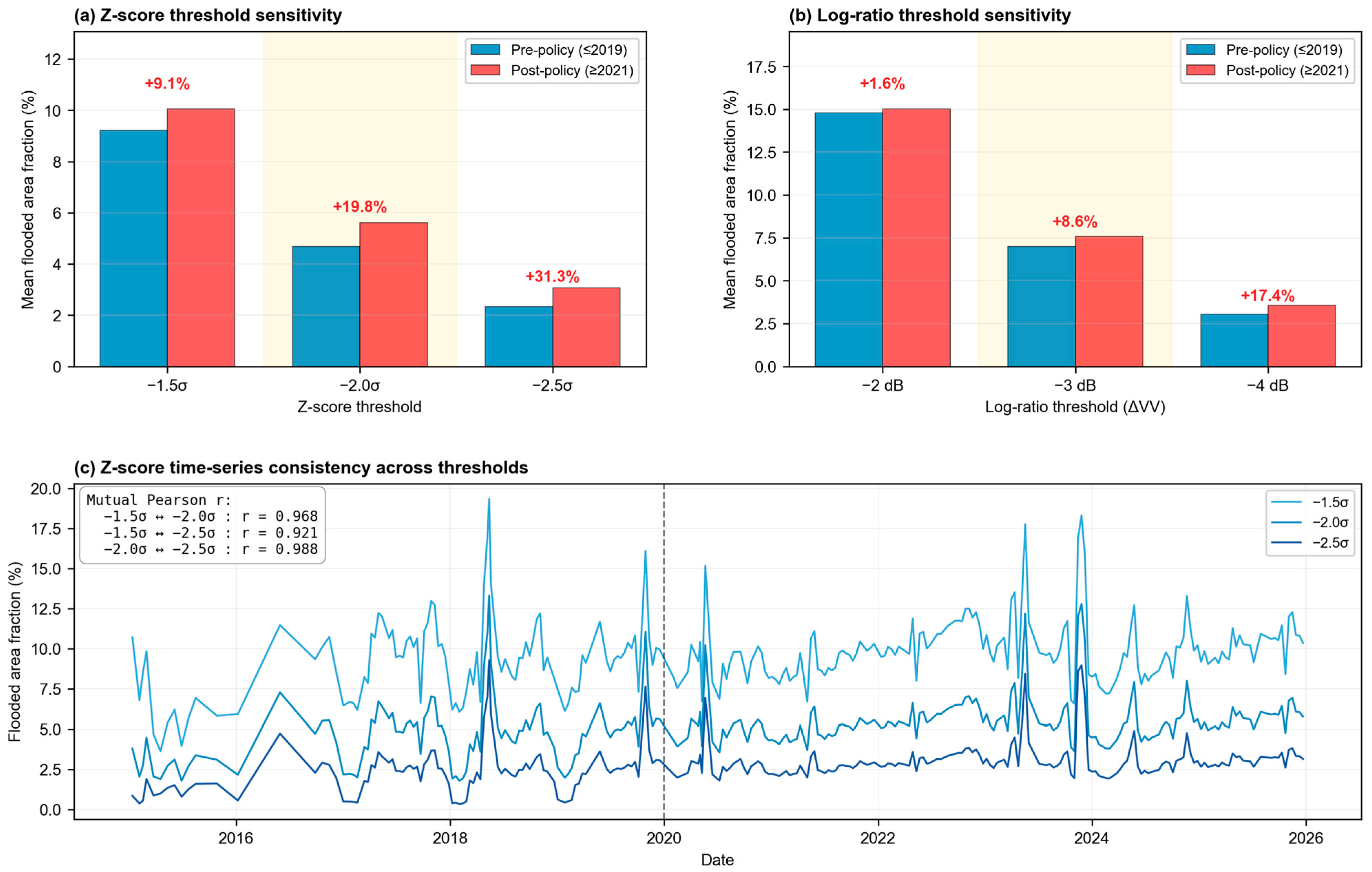
Threshold sensitivity confirmed that the principal conclusions do not depend on the discretionary threshold choice (Figure A4). The post-policy increase was positive at every tested threshold (Z-score: +9.1%/+19.8%/+31.3% at −1.5/−2.0/−2.5σ; log-ratio: +1.6%/+8.6%/+17.4% at −2/−3/−4 dB), and the precipitation coupling remained positive throughout (Z-score Pearson r = +0.25 to +0.38), strengthening at stricter thresholds. Z-score time series at different thresholds were near-identical (mutual r ≥ 0.97), indicating that the threshold affects the absolute flooded area but not the temporal pattern.

3.5. Independent Spatial Consistency and Validation Limitations

Pixel-level validation against optical water masks proved unsuitable in this environment. For the 2019 Deyr flood—among the largest in the record—only 40.8% of Sentinel-2 pixels were cloud-free, and high suspended sediment turbidity suppressed NDWI such that fewer than 16,000 pixels exceeded NDWI > 0 despite extensive inundation; SAR-flagged flood pixels had a median NDWI of −0.31, reflecting the conceptual mismatch between change-based SAR detection and instantaneous optical water. The multi-year JRC GSW product was likewise inadequate as a pixel-level reference: maximum occurrence reached only 35%, with no pixels exceeding 50%, confirming that the Wabi Shabelle here is a seasonal river without a stable permanent water surface.
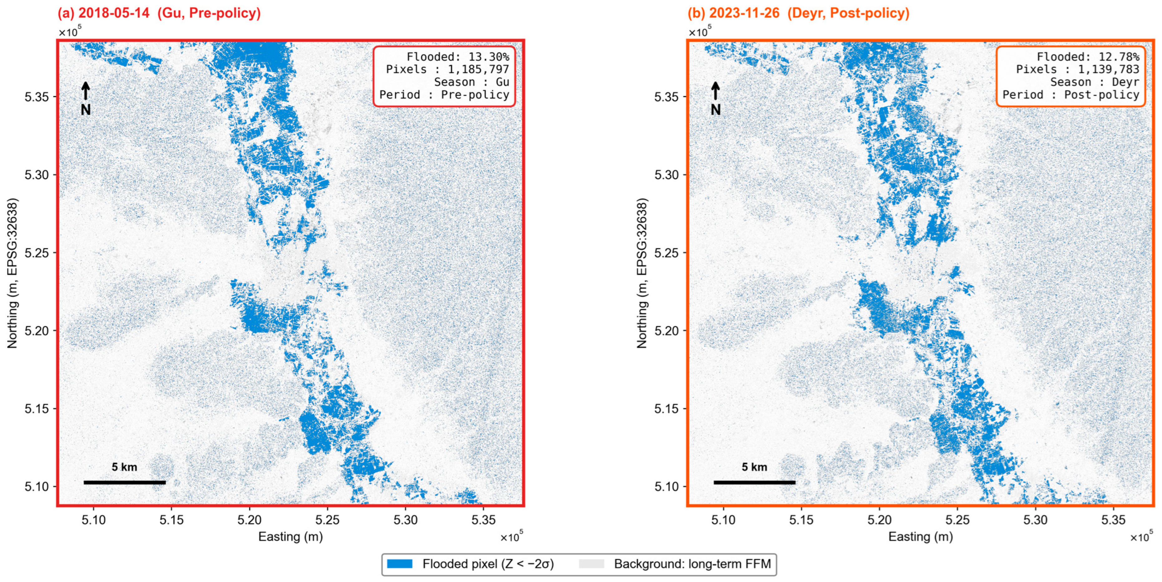
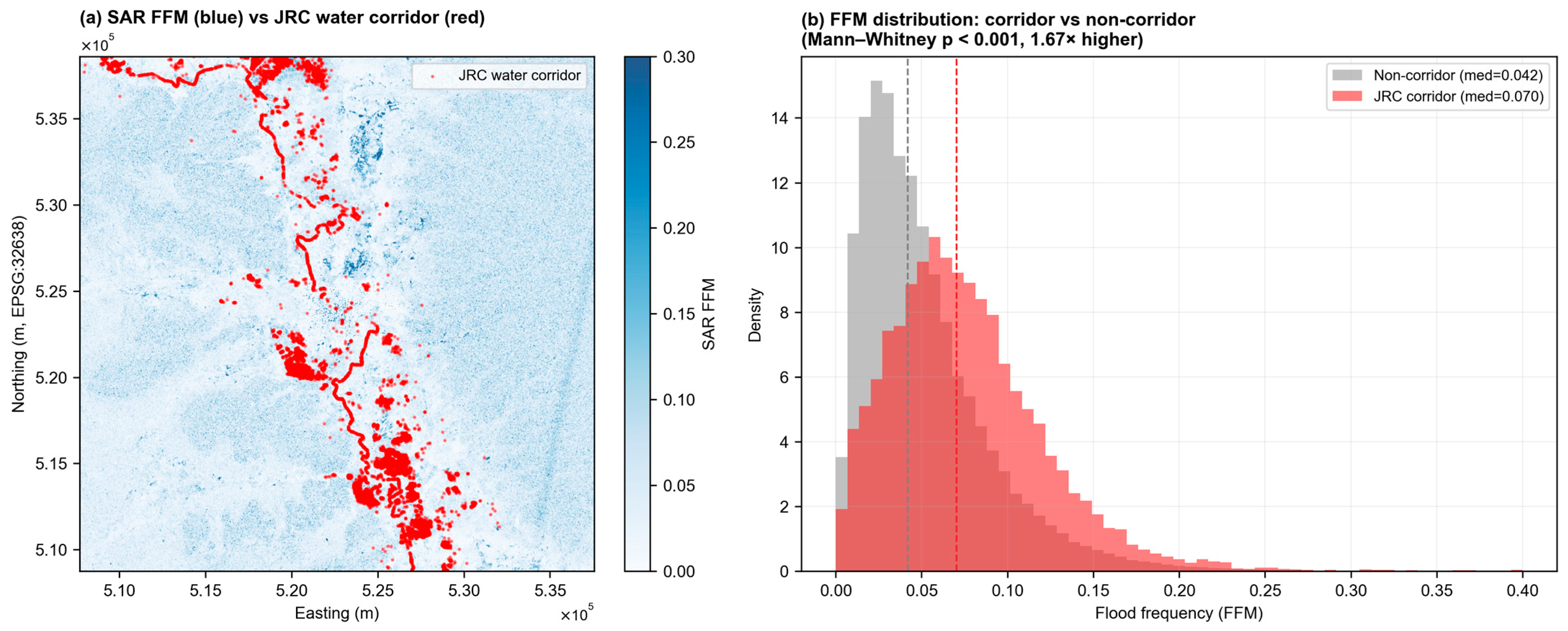
We therefore evaluated independent spatial consistency rather than pixel accuracy. SAR flood frequency was significantly higher within the JRC water corridor (pixels ever observed as water) than outside it (median FFM 0.070 vs. 0.042, a 1.67× difference; Mann–Whitney p < 0.001; Figure A3), and the FFM high-frequency network visually traced the JRC-mapped river corridor. The spatial pattern of the two largest events (2018 Gu and 2023 Deyr) further coincided with the main channel and adjacent floodplain (Appendix A Figure A6). These results indicate that the SAR flood frequency is spatially consistent with independent water observations, while we explicitly caution that the absence of a stable optical reference precludes a conventional precision/recall accuracy figure in this setting.

3.6. Monthly Flood-Area Dynamics and Major Events

Monthly flooded area series (Figure 6a) showed that all major rainfall peaks coincided with flooded area spikes under the Z-score and log-ratio methods. Five major events were identified (2018 Gu, 2019 Deyr, 2020 Gu, 2023 Gu, 2023 Deyr). Annual peak floods under the Z-score method occurred on 14 May 2018 (13.30%), 30 October 2019 (11.04%), 21 May 2020 (10.21%), and the record 26 November 2023 event (12.78%), the last coinciding with the highest monthly CHIRPS total (243.8 mm, November 2023). The log-ratio method gave consistent timing with slightly larger magnitudes, while the fixed-threshold method showed large anti-correlated excursions during dry periods, again illustrating its unsuitability (cf. Section 3.1).

4. Discussion

4.1. Why the Fixed −17 dB Threshold Fails in Semi-Arid Beledweyne

Our results provide strong empirical confirmation that the conventional fixed −17 dB threshold is unsuitable for operational flood mapping in semi-arid East African floodplains. The negative correlation between fixed-threshold flooded area and 12-day precipitation (r = −0.248) is physically implausible and indicates that the method detects a signal opposite to water—most likely persistent dry-sand and bare-soil pixels whose low backscatter dominates the −17 dB classification during dry conditions and partially diminishes (through surface roughening or moisture increase) during rainy periods. This aligns with Martinis et al. [3], who showed that dry sand in Somalia/Ethiopia exhibits backscatter overlapping with open water, and with Wagner et al. [17], who documented anomalous C-band subsurface scattering in arid soils. The lack of agreement between fixed-threshold and Z-score FFM (r = −0.044) further confirms that the two methods detect fundamentally different surface types, with direct implications for the reliability of monitoring systems that uncritically adopt globally calibrated thresholds in arid contexts.
The Z-score method’s positive coupling with rainfall (r = +0.338; bootstrap CI [+0.13, +0.49]) and its agreement with the log-ratio method (r = +0.676) indicate that per-pixel normalization against a dry-season baseline successfully isolates inundation signals from persistent low-backscatter land. This is consistent with the adaptive SAR change-detection literature [14,23,24,62], and our threshold sensitivity analysis shows the result is not contingent on the specific −2σ cut: the precipitation coupling remained positive across thresholds and strengthened at stricter cuts, while the temporal pattern was essentially invariant (mutual r ≥ 0.97). Our results extend this evidence to the semi-arid East African context, where the literature remains sparse.

4.2. DEM Choice and HAND Performance in Semi-Arid Floodplains

Whereas earlier DEM comparisons in mountainous Kathmandu [42] reported substantial FABDEM–GLO-30 differences for HAND-based mapping, we found near-equivalence in Beledweyne: the median pairwise HAND difference between GLO-30 and FABDEM was 0.13 m, with 59% of pixels within 1 m, while SRTM differed more (RMSE ~4.5 m), as expected from its noise. This likely reflects the gentle topography (mean slope < 2°) and minimal vegetation of the Wabi Shabelle floodplain, which reduces the FABDEM vegetation-correction advantage seen in forested or urban terrain. To our knowledge, this is the first empirical FABDEM-HAND evaluation in an East African floodplain, partially filling the gap identified by Meadows et al. [41]. The practical implication is favorable for resource-constrained agencies: freely available GLO-30 can support HAND-based susceptibility mapping at a quality statistically close to FABDEM in low-relief Horn of Africa terrain.
The positive HAND–FFM association (ρ ≈ +0.30) warrants careful interpretation. Mean flood frequency increased with HAND because the permanently wet channel (very low HAND) is registered as temporally unchanged by the change-based detector and therefore exhibits low frequency, whereas transient inundation concentrates across the surrounding floodplain. HAND thus captures fluvial proximity but is a non-monotonic proxy for inundation occurrence in this setting, where overland flow paths also govern flooding [37,38,39]. Rather than undermining the framework, this clarifies the complementary roles of the two layers: the SAR-derived FFM records where water actually recurs, while HAND provides an independent, terrain-based plausibility check; their agreement along the river corridor (and with the independent JRC water corridor, Section 3.5) supports the FFM as a defensible evidence base for terrain-aware land-use planning.

4.3. The 2020 Relocation Policy and Re-Encroachment Evidence

The most policy-relevant finding is that despite the 2020 relocation effort, mean flooded area exposure increased by +19.8% (95% CI 9.1–32.0) in the post-policy period, with BFAST changepoints strongly concentrated in high-flood-frequency pixels (median FFM 4.33× the regional median; KS D = 0.854, p < 0.001). Critically, this increase is not an artefact of rainfall variability: it remained positive and significant after controlling for 12-day precipitation (+0.96 pp, p < 0.001) and after excluding the extreme 2023 events (+0.81 pp, p < 0.001), and it was most pronounced under ordinary low-to-moderate rainfall. Because flood events can themselves generate breakpoints, we do not rest the interpretation on breakpoint timing alone; rather, the inference draws on the convergence of three independent lines of evidence—a precipitation-controlled increase in flooded area fraction, the post-2020 dominance of breakpoints, and their concentration in high-FFM pixels.
We are explicit about what these remote-sensing observations can and cannot establish. They document a sustained increase in floodplain inundation occurrence co-located with the highest-risk zones; they cannot, on their own, identify individual returnees or distinguish returning displaced households from other surface change. The convergent evidence is therefore consistent with, and suggestive of, re-encroachment of populations into hazardous floodplains rather than direct proof of it. So framed, the result indicates that the resettlement intervention as implemented has not delivered durable reduction in floodplain occupancy (SDG 11.5, SDG 13.1).
This pattern is consistent with global evidence that resettlement schemes failing to address underlying vulnerabilities (land access, livelihoods, affordability, governance) frequently result in return migration to hazard zones [10,11,12,13]. Andreadis et al. [8] document that floodplain urban expansion is fastest in the most hazardous zones globally, and De Koning and Filatova [9] show that low-income households can become structurally trapped in hazard areas as safer-land prices rise. Our analysis provides the first SAR-based decadal evidence of this dynamic in a Somali floodplain, addressing the gap noted by Ahmed et al. [1] and Momeni et al. [4]. The implication is direct: structural relocation without parallel investment in alternative livelihoods, secure tenure on safer ground, and inclusive flood risk governance is unlikely to durably reduce flood exposure and may simply displace risk in space and time—a known failure mode of physically framed adaptation that sits uneasily with the “leave no one behind” principle of the 2030 Agenda.

4.4. Validation Constraints in Turbid, Seasonally Dry Rivers

A methodological contribution of this study, surfaced during revision, is the explicit demonstration that standard validation pathways break down in this environment. Optical (Sentinel-2 NDWI) references are suppressed by rainy-season cloud and high turbidity, so that even major floods are barely registered as open water, and the instantaneous optical water signal is conceptually distinct from change-based SAR detection. Multi-year surface water products (JRC GSW) cannot supply a permanent-water reference because the river is seasonal (occurrence ≤ 35%). We therefore validated by independent spatial consistency—SAR flood frequency is significantly elevated within the JRC water corridor (1.67×, p < 0.001) and traces the mapped channel—while transparently reporting that a conventional precision/recall figure is not attainable here. This constraint is itself a transferable finding for SAR flood studies across semi-arid, sediment-laden basins and motivates future high-resolution or in situ validation.

4.5. Limitations and Future Work

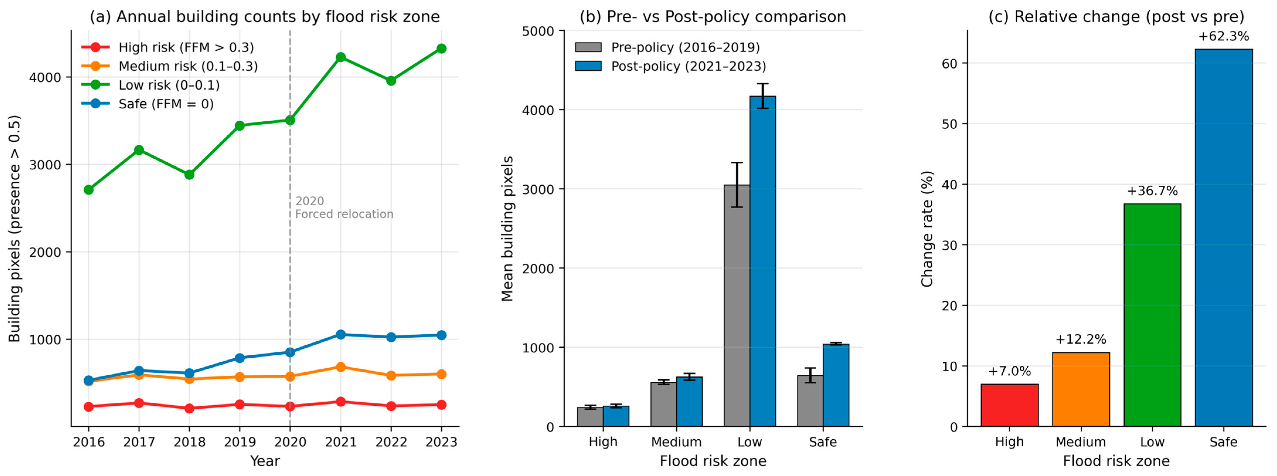
Several limitations remain. First, the FFM captures inundation occurrence, not population or asset exposure directly; coupling FFM with high-resolution population (e.g., WorldPop) and building-footprint layers (e.g., Open Buildings) is a priority and would enable explicit quantification of who is exposed—a preliminary FFM × building overlay (Figure A7) is reported in the Appendix A as a proof of concept. Second, BFAST identifies trend breaks but cannot causally attribute them to specific drivers; longitudinal household surveys, co-designed with affected communities, would be required to confirm re-encroachment at the household level. Third, the Z-score baseline relies on a dry-season pre-policy reference; although chosen to avoid contaminating the change signal, it remains sensitive to the limited number of dry-season scenes, and missing ascending-orbit scenes in 2018–2020 reduce temporal density. Fourth, HAND captures fluvial susceptibility, whereas pluvial and flash flood processes—important in Somali Gu rainfall—would benefit from coupling with hydrodynamic modeling [2,22,38]. Finally, the generalizability of the framework to other Somali floodplains (lower Shabelle, Juba) and other semi-arid East African basins remains to be tested; its fully open-source implementation is intended to lower the barrier to such replication.

5. Conclusions

This study presents the first integrated decadal SAR-based analysis of flood frequency and post-policy floodplain occupancy in Beledweyne, Somalia, framed as an empirical sustainability assessment of a national-scale relocation policy. Beyond its substantive findings, the work delivers several transferable benefits: a fully reproducible, open-source, GEE-based workflow requiring no commercial data; an explicit benchmarking of three flood detection methods that identifies which is trustworthy in semi-arid terrain; the first FABDEM-HAND evaluation in East Africa showing that cost-free GLO-30 suffices; and a robustness suite (precipitation control, bootstrap uncertainty, threshold sensitivity, revisit interval and independent consistency checks) that strengthens confidence in policy-relevant conclusions drawn from EO data.
Three principal conclusions emerge. First, in semi-arid East African floodplains, the conventional fixed −17 dB SAR threshold is unreliable owing to water/dry-sand confusion; per-pixel Z-score change detection yields physically consistent, rainfall-coupled results—stable across thresholds—and should be preferred for operational flood monitoring. Second, in this low-relief, vegetation-sparse setting, Copernicus GLO-30 and FABDEM produce near-equivalent HAND maps, supporting HAND as a transferable, license-free susceptibility proxy for low-income national agencies. Third, BFAST changepoint analysis and a precipitation-controlled pre/post comparison reveal a +19.8% post-2020 increase in flooded area occupancy (95% CI 9.1–32.0; robust to precipitation control and to exclusion of 2023), with breakpoints concentrated in high-flood-frequency pixels (KS D = 0.854, p < 0.001)—a pattern consistent with re-encroachment into hazardous zones despite the 2020 policy.
Taken together, these findings underscore a core sustainability lesson: structural relocation alone is insufficient to durably reduce flood exposure, and a sustainable disaster risk reduction pathway requires complementary investments in tenure security, livelihoods, and inclusive governance, in alignment with SDG 1.5, SDG 11.5, and SDG 13.1. The multi-method, open-source SAR framework developed here is directly transferable to other Horn of Africa floodplains and provides a low-cost monitoring template for evaluating and, where necessary, redesigning future disaster-risk-reduction interventions in data-sparse settings.


Author Contributions

Conceptualization, I.-S.H., J.-S.K., S.-J.L. and H.-S.Y.; methodology, I.-S.H., J.-S.K., S.-J.L. and H.-S.Y.; software, I.-S.H. and S.-J.L.; validation, I.-S.H. and S.-J.L.; formal analysis, I.-S.H. and S.-J.L.; investigation, I.-S.H. and S.-J.L.; resources, H.-S.Y.; data curation, I.-S.H., J.-S.K. and S.-J.L.; writing—original draft preparation, I.-S.H., J.-S.K. and S.-J.L.; writing—review and editing, I.-S.H., S.-J.L. and H.-S.Y.; visualization, I.-S.H. and S.-J.L.; supervision, S.-J.L. and H.-S.Y.; project administration, H.-S.Y.; funding acquisition, J.-S.K., H.-S.Y. All authors have read and agreed to the published version of the manuscript.

Funding

This research was supported by the 2023-MOIS36-004 (RS-2023-00248092) of the Technology Development Program on Disaster Restoration Capacity Building and Strengthening, funded by the Ministry of the Interior and Safety (MOIS, Republic of Korea).

Institutional Review Board Statement

Not applicable.

Informed Consent Statement

Not applicable.

Data Availability Statement

All code (Python modules, Jupyter notebooks) and processed data products supporting this study are openly available on GitHub at https://github.com/lsj794222-stack/beledweyne-flood-ffm (accessed on 29 May 2026) and permanently archived on Zenodo at https://doi.org/10.5281/zenodo.20454490 (accessed on 29 May 2026). The raw Sentinel-1 GRD and Sentinel-2 L2A scenes were accessed through Google Earth Engine (https://earthengine.google.com, accessed on 29 May 2026). CHIRPS daily precipitation, Copernicus GLO-30, FABDEM v1.2, and SRTM GL1 v3 are publicly available via Google Earth Engine catalogues. Administrative boundaries (GADM v4.1) and hydrography (HOTOSM Somalia, OpenStreetMap) are available from their respective providers.

Conflicts of Interest

The authors declare no conflicts of interest.

Abbreviations

The following abbreviations are used in this manuscript:
BFASTBreaks For Additive Season and Trend
CHIRPSClimate Hazards Group InfraRed Precipitation with Station data
CIConfidence interval
DEMDigital elevation model
FABDEMForest And Buildings removed Copernicus DEM
FFMFlood frequency metric
GADMDatabase of Global Administrative Areas
GEEGoogle Earth Engine
GLO-30Copernicus Global Digital Elevation Model at 30 m resolution
GRDGround Range Detected (Sentinel-1 product)
HANDHeight Above Nearest Drainage
HOTOSMHumanitarian OpenStreetMap Team
IWInterferometric Wide (Sentinel-1 swath mode)
KSKolmogorov–Smirnov (two-sample test)
MAEMean absolute error
NDWINormalized Difference Water Index
RMSERoot mean square error
ROIRegion of interest
SARSynthetic aperture radar
SDGSustainable Development Goal(s)
SRTMShuttle Radar Topography Mission
VVVertical–vertical polarization

Appendix A

Figure A1. Quality control and replacement of one anomalous Sentinel-1 T1A scene (30 July 2018, ascending orbit). (a) VV backscatter map of the re-exported replacement scene with complete spatial coverage. (b) Log-scale VV distribution comparison between the truncated original (OLD, red; n = 54,144; 0.61% coverage; mean = −12.87 dB) and the re-exported scene (NEW, blue; n = 8,926,928; 99.95% coverage; mean = −11.16 dB). Dashed lines mark distribution means; the dotted line indicates the fixed −17 dB threshold. The mean difference of −1.71 dB, weighted by the scene’s 1/115 contribution to the reference composite, yields a residual impact below 0.02 dB, confirming replacement adequacy.
Sustainability 18 07060 g0a1
Figure A2. Pairwise HAND differences between the three digital elevation models used in Section 3.2. (a) Copernicus GLO-30 minus FABDEM, (b) GLO-30 minus SRTM, and (c) FABDEM minus SRTM, shown as spatial ΔHAND maps in meters. (d) Pixel-wise distributions of the three difference layers on a logarithmic count scale. GLO-30 and FABDEM are near-equivalent in this low-relief setting (median ΔHAND = 0.13 m; mean = 0.04 m; 59.0% of pixels within 1 m), whereas both SRTM-based pairs show substantially broader dispersion and heavier tails (RMSE 4.4–4.5 m; only ~33% of pixels within 1 m), consistent with the documented SRTM noise noted in Section 3.2. Full pairwise statistics are reported in Table A2.
Sustainability 18 07060 g0a2
Figure A3. Independent spatial consistency between SAR-derived flood frequency and the JRC Global Surface Water product. (a) Flood frequency metric (FFM, blue intensity) overlaid with the JRC water corridor (red; pixels ever observed as water). (b) FFM distribution inside versus outside the corridor, showing 1.67× higher median FFM within the JRC corridor (0.070 versus 0.042; Mann–Whitney U test, p < 0.001). Because the Wabi Shabelle here is a seasonal river without a stable permanent water surface, this spatial consistency check substitutes for a conventional pixel-level accuracy assessment (Section 3.5).
Sustainability 18 07060 g0a3
Figure A4. Threshold sensitivity analysis of the Z-score and log-ratio flood detection methods, addressing the potentially discretionary nature of the adopted thresholds. (a) Mean flooded area fraction under three Z-score thresholds (−1.5σ, −2.0σ, −2.5σ) for pre-policy (≤2019) versus post-policy (≥2021) periods, showing that the post-policy increase is positive and monotonically strengthening with stricter thresholds (+9.1%/+19.8%/+31.3%). (b) Same comparison for three log-ratio thresholds (−2, −3, −4 dB), yielding similarly monotonic positive increases (+1.6%/+8.6%/+17.4%). (c) Daily flooded area fraction time series for the three Z-score thresholds, with adjacent-threshold Pearson correlations of r = 0.97–0.99 (r = 0.968 for −1.5σ/−2.0σ; r = 0.988 for −2.0σ/−2.5σ) and full-range r = 0.921, confirming that the temporal signal is essentially threshold-invariant. The adopted thresholds (Z < −2.0σ; ΔVV < −3 dB), highlighted in gold, represent the mid-range values whose pre-policy flooded fractions (4.7% and 7.0%, respectively) correspond to physically plausible flood extents for this semi-arid setting (Section 2.4.3 and Section 2.4.4). Full sensitivity results are discussed in Section 2.8 and Section 3.4.
Sustainability 18 07060 g0a4
Figure A5. Bootstrap uncertainty of the post-policy flood-exposure increase. (a) Bootstrap distributions (10,000 resamples) of the pre-policy (blue; mean = 4.68%, 95% CI 4.30–5.10) and post-policy (red; mean = 5.61%, 95% CI 5.39–5.87) Z-score flooded area fractions. (b) Distribution of the relative change Δ = (post − pre)/pre × 100%. The bootstrap mean (+20.1%) is closely consistent with the observed point estimate (+19.8%; Section 3.3), and the 95% CI [9.1, 32.0] excludes zero (black line), confirming that the post-policy increase is statistically significant. The vertical red line marks the bootstrap mean; the shaded band shows the 95% CI.
Sustainability 18 07060 g0a5
Figure A6. Maximum flood inundation extent before versus after the 2020 relocation policy. SAR Z-score flood masks (Z < −2σ, blue) overlaid on the long-term flood frequency metric (FFM, grey background) for the largest pre-policy event ((a): 14 May 2018 Gu flood, 13.30% flooded, 1,185,797 pixels) and the largest post-policy event ((b): 26 November 2023 Deyr flood, 12.78% flooded, 1,139,783 pixels; associated with November 2023 monthly CHIRPS peak of 243.8 mm). The two events yield near-identical floodplain footprints, indicating that the SAR method captures consistent spatial inundation patterns across the pre- and post-policy periods regardless of season, and supporting the validity of the SAR-based flood detection framework in the absence of a stable pixel-level optical reference (Section 3.5).
Sustainability 18 07060 g0a6
Figure A7. Preliminary FFM × building overlay as a proof-of-concept demonstration of coupling the SAR-derived flood frequency metric (FFM) with independent building-footprint data (Section 4.5). Buildings are classified into four flood risk zones by their long-term FFM value: high risk (FFM > 0.3), medium risk (0.1–0.3), low risk (0–0.1), and safe (FFM = 0). (a) Annual building-pixel counts (presence > 0.5) by risk zone from 2016 to 2023; the dashed vertical line marks the 2020 forced-relocation policy. (b) Pre-policy (2016–2019) versus post-policy (2021–2023) mean building pixels per zone, with error bars indicating inter-annual standard deviations. (c) Relative change in mean building pixels between the two periods (+7.0%, high; +12.2%, medium; +36.7%, low; +62.3%, safe). Critically, building density continued to increase in the high- and medium-risk zones despite the 2020 relocation policy, consistent with the SAR-based evidence of re-encroachment presented in the main text; the larger increases in low-risk and safe zones reflect concurrent urban growth outside the immediate floodplain. Because the underlying building-footprint layer has not been independently validated against ground-truth surveys, these results are reported as a proof of concept, and quantitative attribution of individual settlements to specific risk categories requires further validation (Section 4.5).
Sustainability 18 07060 g0a7
Table A1. Quality-control summary and statistics for the replaced Sentinel-1 scene (2018-07-30).
MetricOLD (Truncated)NEW (Re-Exported)Difference/Ratio
Acquisition date30 July 201830 July 2018
Orbit directionAscendingAscendingIdentical
Valid pixel count54,1448,926,928×165
Valid coverage (%)0.6199.95+99.34 pp
Mean VV (dB)−12.87−11.16−1.71
Distribution shapeTruncated (low-backscatter biased)Full semi-arid regime
Scene weight in composite1/1151/115
Impact on composite mean<0.02 dB
QC decisionRejectedRetained
Notes: The OLD scene was rejected due to spatial truncation at the Google Earth Engine export stage. The residual impact of the replacement on the long-term reference composite mean is below 0.02 dB, confirming that the substitution does not compromise downstream Z-score and log-ratio analyses (Figure A1). pp = percentage points.
Table A2. Pairwise HAND difference statistics between DEMs (mean, median, MAE, RMSE, % within 1 m).
DEM PairMean (m)Median Signed (m)Median |Δ| (m)Std (m)MAE (m)RMSE (m)P95 |Δ| (m)Within ±1 m (%)
GLO-30−FABDEM0.040.130.753.131.623.136.3159
GLO-30−SRTM0.40.111.824.392.824.418.6133.1
FABDEM−SRTM0.360.051.814.462.844.488.8533.6
Notes: MAE = mean absolute error; RMSE = root mean square error; P95 |Δ| = 95th percentile of absolute difference. GLO-30 and FABDEM are near-equivalent in this low-relief setting (59.0% within ±1 m), whereas both SRTM-based pairs show broader dispersion and heavier tails (~33% within ±1 m; RMSE 4.4–4.5 m), consistent with SRTM’s documented noise (Section 3.2; Figure A2).
Table A3. Sentinel-1 revisit interval and seasonal-sampling summary, and block-bootstrap 95% CI for the precipitation–flood correlation.
CategoryParameter/ItemValueNotes
AcquisitionTotal scenes (descending)259Ascending-orbit scenes excluded (Section 2.4.1)
AcquisitionStudy periodJanuary 2015–June 202510-year archive
AcquisitionMedian revisit interval (days)12Native S-1 revisit under single-orbit config.
AcquisitionFraction of intervals ≤36 days (%)94.6Confirms low temporal gap frequency
Seasonal samplingWet season (April–June, October–December)n = 130 (50.2%)Gu + Deyr rainy seasons
Seasonal samplingDry season (January–March, July–September)n = 129 (49.8%)Jilaal + Hagaa dry seasons
Seasonal samplingWet/dry balance1.008: 1.000No seasonal sampling bias (Section 3.4)
Precip. couplingZ-score—CHIRPS 12-day Pearson r+0.338Section 3.1, Section 3.4
Precip. couplingZ-score block-bootstrap 95% CI[+0.13, +0.49]Excludes zero; autocorrelation-aware
Precip. couplingLog-ratio—CHIRPS 12-day Pearson r+0.209Point estimate; CI not computed
Precip. couplingFixed −17 dB—CHIRPS 12-day Pearson r−0.248Negative coupling (method invalid; Section 4.1)
Notes: The block-bootstrap procedure was applied with autocorrelation-aware blocks to account for the irregular Sentinel-1 revisit interval. The Z-score precipitation correlation is statistically significant and robust to temporal autocorrelation, with the 95% CI [+0.13, +0.49] excluding zero (Section 3.1 and Section 3.4). The near-balanced wet/dry sampling (50.2% vs 49.8%) confirms no seasonal bias that could spuriously inflate the correlation.

References

  1. Ahmed, M.; Asowe, H.; Dirie, N.; Mohamud, A.; Lucero-Prisno, D.; Okesanya, O.; Ogaya, J.; Musa, S.; Musa, M.; Othman, Z.; et al. The Nexus of Climate Change, Food Insecurity, and Conflict in Somalia. F1000Research 2024, 13, 921. [Google Scholar] [CrossRef]
  2. Ibrahim, O.; Goshime, D.; Gebrekirtos, S.; Absi, R. Flood inundation mapping and mitigation options in data-scarce region of Beledwayne town in the Wabi Shebele River Basin of Somalia. Nat. Hazards Res. 2024, 4, 336–346. [Google Scholar] [CrossRef]
  3. Martinis, S.; Plank, S.; Cwik, K. The Use of Sentinel-1 Time-Series Data to Improve Flood Monitoring in Arid Areas. Remote Sens. 2018, 10, 583. [Google Scholar] [CrossRef]
  4. Momeni, R.; Bircan, T.; King, R.; Santos, E. Deciphering climate-induced displacement in Somalia: A remote sensing perspective. PLoS ONE 2024, 19, e0304202. [Google Scholar] [CrossRef] [PubMed]
  5. Yuen, A.; Warsame, A.; Checchi, F. Exploring the temporal patterns and crisis-related risk factors for population displacement in Somalia (2016–2018). J. Migr. Health 2022, 5, 100095. [Google Scholar] [CrossRef] [PubMed]
  6. Oh, W.; Muneepeerakul, R.; Rubenstein, D.; Levin, S. Emergent network patterns of internal displacement in Somalia driven by natural disasters and conflicts. Glob. Environ. Change 2024, 84, 102793. [Google Scholar] [CrossRef]
  7. Osman, A.; Abebe, G. Rural Displacement and Its Implications on Livelihoods and Food Insecurity: The Case of Inter-Riverine Communities in Somalia. Agriculture 2023, 13, 1444. [Google Scholar] [CrossRef]
  8. Andreadis, K.; Wing, O.; Colven, E.; Gleason, C.; Bates, P.; Brown, C. Urbanizing the floodplain: Global changes of imperviousness in flood-prone areas. Environ. Res. Lett. 2021, 17, 104024. [Google Scholar] [CrossRef]
  9. De Koning, K.; Filatova, T. Repetitive floods intensify outmigration and climate gentrification in coastal cities. Environ. Res. Lett. 2020, 15, 034008. [Google Scholar] [CrossRef]
  10. Kita, S. Urban vulnerability, disaster risk reduction and resettlement in Mzuzu city, Malawi. Int. J. Disaster Risk Reduct. 2017, 22, 158–166. [Google Scholar] [CrossRef]
  11. Mashi, S.; Inkani, A.; Obaro, O.; Asanarimam, A. Community perception, response and adaptation strategies towards flood risk in a traditional African city. Nat. Hazards 2020, 103, 1727–1759. [Google Scholar] [CrossRef]
  12. Wagner, S.; Souvignet, M.; Walz, Y.; Balogun, K.; Komi, K.; Kreft, S.; Rhyner, J. When does risk become residual? A systematic review of research on flood risk management in West Africa. Reg. Environ. Change 2021, 21, 84. [Google Scholar] [CrossRef] [PubMed]
  13. Awah, L.; Belle, J.; Nyam, Y.; Orimoloye, I. A Systematic Analysis of Systems Approach and Flood Risk Management Research. Int. J. Disaster Risk Sci. 2024, 15, 45–57. [Google Scholar] [CrossRef]
  14. Lang, F.; Zhu, Y.; Zhao, J.; Hu, X.; Shi, H.; Zheng, N.; Zha, J. Flood Mapping of Synthetic Aperture Radar (SAR) Imagery Based on Semi-Automatic Thresholding and Change Detection. Remote Sens. 2024, 16, 2763. [Google Scholar] [CrossRef]
  15. Colacicco, R.; Refice, A.; Nutricato, R.; Bovenga, F.; Caporusso, G.; D’Addabbo, A.; Salandra, M.; Lovergine, F.; Nitti, D.; Capolongo, D. High-Resolution Flood Monitoring Based on Advanced Statistical Modeling of Sentinel-1 Multi-Temporal Stacks. Remote Sens. 2024, 16, 294. [Google Scholar] [CrossRef]
  16. Giustarini, L.; Hostache, R.; Matgen, P.; Schumann, G.; Bates, P.; Mason, D. A Change Detection Approach to Flood Mapping in Urban Areas Using TerraSAR-X. IEEE Trans. Geosci. Remote Sens. 2013, 51, 2417–2430. [Google Scholar] [CrossRef]
  17. Wagner, W.; Lindorfer, R.; Melzer, T.; Hahn, S.; Bauer-Marschallinger, B.; Morrison, K.; Calvet, J.; Hobbs, S.; Quast, R.; Greimeister-Pfeil, I.; et al. Widespread occurrence of anomalous C-band backscatter signals in arid environments caused by subsurface scattering. Remote Sens. Environ. 2022, 276, 113025. [Google Scholar] [CrossRef]
  18. Notti, D.; Giordan, D.; Calò, F.; Pepe, A.; Zucca, F.; Galve, J. Potential and Limitations of Open Satellite Data for Flood Mapping. Remote Sens. 2018, 10, 1673. [Google Scholar] [CrossRef]
  19. Tran, K.; Menenti, M.; Jia, L. Surface Water Mapping and Flood Monitoring in the Mekong Delta Using Sentinel-1 SAR Time Series and Otsu Threshold. Remote Sens. 2022, 14, 5721. [Google Scholar] [CrossRef]
  20. Lin, Y.; Yun, S.; Bhardwaj, A.; Hill, E. Urban Flood Detection with Sentinel-1 Multi-Temporal Synthetic Aperture Radar (SAR) Observations in a Bayesian Framework: A Case Study for Hurricane Matthew. Remote Sens. 2019, 11, 1778. [Google Scholar] [CrossRef]
  21. Cao, H.; Zhang, H.; Wang, C.; Zhang, B. Operational Flood Detection Using Sentinel-1 SAR Data over Large Areas. Water 2019, 11, 786. [Google Scholar] [CrossRef]
  22. Liang, J.; Liu, D. A local thresholding approach to flood water delineation using Sentinel-1 SAR imagery. ISPRS J. Photogramm. Remote Sens. 2019, 159, 53–62. [Google Scholar] [CrossRef]
  23. Elkhrachy, I.; Pham, Q.; Costache, R.; Mohajane, M.; Rahman, K.; Shahabi, H.; Linh, N.; Anh, D. Sentinel-1 remote sensing data and HEC-RAS two-dimensional integration for flash flood detection and modelling in New Cairo City, Egypt. J. Flood Risk Manag. 2021, 14, e12692. [Google Scholar] [CrossRef]
  24. Jarrett, S.; Hölbling, D. Spatial Evaluation of a Natural Flood Management Project Using SAR Change Detection. Water 2023, 15, 2182. [Google Scholar] [CrossRef]
  25. Amitrano, D.; Martino, G.; Simone, A.; Imperatore, P. Flood Detection with SAR: A Review of Techniques and Datasets. Remote Sens. 2024, 16, 656. [Google Scholar] [CrossRef]
  26. Bekele, T.; Haile, A.; Trigg, M.; Walsh, C. Evaluating a new method of remote sensing for flood mapping in the urban and peri-urban areas: Applied to Addis Ababa and the Akaki catchment in Ethiopia. Nat. Hazards Res. 2022, 2, 97–110. [Google Scholar] [CrossRef]
  27. Mohsenifar, A.; Mohammadzadeh, A.; Jamali, S. Unsupervised Rural Flood Mapping from Bi-Temporal Sentinel-1 Images Using an Improved Wavelet-Fusion Flood-Change Index (IWFCI) and an Uncertainty-Sensitive Markov Random Field (USMRF) Model. Remote Sens. 2025, 17, 1024. [Google Scholar] [CrossRef]
  28. Haile, A.; Bekele, T.; Rientjes, T. Interannual comparison of historical floods through flood detection using multi-temporal Sentinel-1 SAR images, Awash River Basin, Ethiopia. Int. J. Appl. Earth Obs. Geoinf. 2023, 124, 103505. [Google Scholar] [CrossRef]
  29. Vanama, V.; Rao, Y.; Bhatt, C. Change detection based flood mapping using multi-temporal Earth Observation satellite images: 2018 flood event of Kerala, India. Eur. J. Remote Sens. 2021, 54, 42–58. [Google Scholar] [CrossRef]
  30. Wu, X.; Zhang, Z.; Xiong, S.; Zhang, W.; Tang, J.; Li, Z.; An, B.; Li, R. A Near-Real-Time Flood Detection Method Based on Deep Learning and SAR Images. Remote Sens. 2023, 15, 2046. [Google Scholar] [CrossRef]
  31. Diehl, R.; Gourevitch, J.; Drago, S.; Wemple, B. Improving flood hazard datasets using a low-complexity, probabilistic floodplain mapping approach. PLoS ONE 2021, 16, e0248683. [Google Scholar] [CrossRef] [PubMed]
  32. Unnithan, S.; Biswal, B.; Sharples, W.; Rüdiger, C.; Bahramian, K.; Hou, J. Sensitivity Analysis of Modelled Flood Inundation Extents over Hawkesbury–Nepean Catchment. Geosciences 2023, 13, 67. [Google Scholar] [CrossRef]
  33. Thalakkottukara, N.; Thomas, J.; Watkins, M.; Holland, B.; Oommen, T.; Grover, H. Suitability of the height above nearest drainage (HAND) model for flood inundation mapping in data-scarce regions. Earth Sci. Inform. 2024, 17, 1907–1921. [Google Scholar] [CrossRef]
  34. Aristizabal, F.; Salas, F.; Petrochenkov, G.; Grout, T.; Avant, B.; Bates, B.; Spies, R.; Chadwick, N.; Wills, Z.; Judge, J. Extending Height Above Nearest Drainage to Model Multiple Fluvial Sources in Flood Inundation Mapping Applications for the U.S. National Water Model. Water Resour. Res. 2023, 59, e2022WR032039. [Google Scholar] [CrossRef]
  35. Chaudhuri, C.; Gray, A.; Robertson, C. InundatEd-v1.0: A height above nearest drainage (HAND)-based flood risk modeling system using a discrete global grid system. Geosci. Model Dev. 2021, 14, 3295–3315. [Google Scholar] [CrossRef]
  36. Li, Z.; Duque, F.; Grout, T.; Bates, B.; Demir, I. Comparative analysis of performance and mechanisms of flood inundation map generation using Height Above Nearest Drainage. Environ. Model. Softw. 2022, 159, 105565. [Google Scholar] [CrossRef]
  37. Zheng, X.; Maidment, D.; Tarboton, D.; Liu, Y.; Passalacqua, P. GeoFlood: Large-Scale Flood Inundation Mapping Based on High-Resolution Terrain Analysis. Water Resour. Res. 2018, 54, 10013–10033. [Google Scholar] [CrossRef]
  38. Afshari, S.; Tavakoly, A.; Rajib, M.; Zheng, X.; Follum, M.; Omranian, E.; Fekete, B. Comparison of new generation low-complexity flood inundation mapping tools with a hydrodynamic model. J. Hydrol. 2017, 556, 539–556. [Google Scholar] [CrossRef]
  39. Vojtek, M.; Moradi, S.; Petroselli, A.; Vojteková, J. Comparative analysis of hydraulic and GIS-based Height Above the Nearest Drainage model for fluvial flood hazard mapping: A case of the Gidra River, Slovakia. Stoch. Environ. Res. Risk Assess. 2025, 39, 2657–2675. [Google Scholar] [CrossRef]
  40. Aristizabal, F.; Chegini, T.; Petrochenkov, G.; Salas, F.; Judge, J. Effects of high-quality elevation data and explanatory variables on the accuracy of flood inundation mapping via Height Above Nearest Drainage. Hydrol. Earth Syst. Sci. 2024, 28, 1287–1310. [Google Scholar] [CrossRef]
  41. Meadows, M.; Jones, S.; Reinke, K. Vertical accuracy assessment of freely available global DEMs (FABDEM, Copernicus DEM, NASADEM, AW3D30 and SRTM) in flood-prone environments. Int. J. Digit. Earth 2024, 17, 2308734. [Google Scholar] [CrossRef]
  42. Watson, C.; Gyawali, J.; Creed, M.; Elliott, J. City-scale high-resolution flood models and the role of topographic data: A case study of Kathmandu, Nepal. Geocarto Int. 2024, 39, 2387073. [Google Scholar] [CrossRef]
  43. Verbesselt, J.; Hyndman, R.; Zeileis, A.; Culvenor, D. Phenological change detection while accounting for abrupt and gradual trends in satellite image time series. Remote Sens. Environ. 2010, 114, 2970–2980. [Google Scholar] [CrossRef]
  44. Verbesselt, J.; Hyndman, R.; Newnham, G.; Culvenor, D. Detecting trend and seasonal changes in satellite image time series. Remote Sens. Environ. 2010, 114, 106–115. [Google Scholar] [CrossRef]
  45. Abbes, B.; Bounouh, O.; Farah, I.; De Jong, R.; Martínez, B. Comparative study of three satellite image time-series decomposition methods for vegetation change detection. Eur. J. Remote Sens. 2018, 51, 607–615. [Google Scholar] [CrossRef]
  46. Geng, L.; Che, T.; Wang, X.; Wang, H. Detecting Spatiotemporal Changes in Vegetation with the BFAST Model in the Qilian Mountain Region during 2000–2017. Remote Sens. 2019, 11, 103. [Google Scholar] [CrossRef]
  47. Grogan, K.; Pflugmacher, D.; Hostert, P.; Verbesselt, J.; Fensholt, R. Mapping Clearances in Tropical Dry Forests Using Breakpoints, Trend, and Seasonal Components from MODIS Time Series. Remote Sens. 2016, 8, 657. [Google Scholar] [CrossRef]
  48. Wu, L.; Li, Z.; Liu, X.; Zhu, L.; Tang, Y.; Zhang, B.; Xu, B.; Liu, M.; Meng, Y.; Liu, B. Multi-Type Forest Change Detection Using BFAST and Monthly Landsat Time Series for Monitoring Spatiotemporal Dynamics of Forests in Subtropical Wetland. Remote Sens. 2020, 12, 341. [Google Scholar] [CrossRef]
  49. Vasios, G.; Alexoudaki, E.; Kaloveloni, A.; Troumbis, A. Landsat Time Series Analysis with BFAST for Detecting Degradation of Thyme Shrublands by Fire on Lemnos Island. Fire 2025, 8, 335. [Google Scholar] [CrossRef]
  50. Costa, H.; Giraldo, A.; Caetano, M. Exploring BFAST to detect forest changes in Portugal. In Proceedings of the SPIE Environmental Remote Sensing, Image and Signal Processing for Remote Sensing XXVI; SPIE: Bellingham, WA, USA, 2020; Volume 11533, p. 1153308. [Google Scholar] [CrossRef]
  51. Mendes, M.; Rodriguez-Galiano, V.; Aragones, D. Evaluating the BFAST method to detect and characterise changing trends in water time series: A case study on the impact of droughts on the Mediterranean climate. Sci. Total Environ. 2022, 852, 157428. [Google Scholar] [CrossRef] [PubMed]
  52. Marden, A.; Meyer, T.; Meyer, K. Regional fire occurrence in Southern Africa using BFAST iterative break detection in seasonal and trend components of a MODIS time series. S. Afr. Geogr. J. 2022, 105, 200–221. [Google Scholar] [CrossRef]
  53. Alemayehu, B.; Suarez-Minguez, J.; Rosette, J.; Khan, S. Vegetation Trend Detection Using Time Series Satellite Data as Ecosystem Condition Indicators for Analysis in the Northwestern Highlands of Ethiopia. Remote Sens. 2023, 15, 5032. [Google Scholar] [CrossRef]
  54. Scarpetta, Y.; Lebourgeois, V.; Laques, A.; Dieye, M.; Bourgoin, J.; Bégué, A. BFASTm-L2, an unsupervised LULCC detection based on seasonal change detection—An application to large-scale land acquisitions in Senegal. Int. J. Appl. Earth Obs. Geoinf. 2023, 121, 103379. [Google Scholar] [CrossRef]
  55. Masiliūnas, D.; Tsendbazar, N.; Herold, M.; Verbesselt, J. BFAST Lite: A Lightweight Break Detection Method for Time Series Analysis. Remote Sens. 2021, 13, 3308. [Google Scholar] [CrossRef]
  56. Rhif, M.; Abbes, A.; Martínez, B.; Jong, R.; Sang, Y.; Farah, I. Detection of trend and seasonal changes in non-stationary remote sensing data: Case study of Tunisia vegetation dynamics. Ecol. Inform. 2022, 69, 101596. [Google Scholar] [CrossRef]
  57. Li, J.; Li, Z.; Wu, H.; You, N. Trend, seasonality, and abrupt change detection method for land surface temperature time-series analysis: Evaluation and improvement. Remote Sens. Environ. 2022, 280, 113222. [Google Scholar] [CrossRef]
  58. Ghaderpour, E.; Vujadinovic, T. Change Detection within Remotely Sensed Satellite Image Time Series via Spectral Analysis. Remote Sens. 2020, 12, 4001. [Google Scholar] [CrossRef]
  59. Watts, L.; Laffan, S. Effectiveness of the BFAST algorithm for detecting vegetation response patterns in a semi-arid region. Remote Sens. Environ. 2014, 154, 234–245. [Google Scholar] [CrossRef]
  60. Murakami, T.; Tsutsumida, N. Comparative Global Assessment and Optimization of LandTrendr, CCDC, and BFAST Algorithms for Enhanced Urban Land Cover Change Detection Using Landsat Time Series. Remote Sens. 2025, 17, 2402. [Google Scholar] [CrossRef]
  61. Pekel, J.-F.; Cottam, A.; Gorelick, N.; Belward, A.S. High-resolution mapping of global surface water and its long-term changes. Nature 2016, 540, 418–422. [Google Scholar] [CrossRef] [PubMed]
  62. Katiyar, V.; Tamkuan, N.; Nagai, M. Near-Real-Time Flood Mapping Using Off-the-Shelf Models with SAR Imagery and Deep Learning. Remote Sens. 2021, 13, 2334. [Google Scholar] [CrossRef]
Figure 1. Study area of Beledweyne, Hiraan Region, Somalia. (a) Location of Somalia within Africa; (b) the Hiraan Region and Beledweyne within Somalia, with Mogadishu shown for reference. Somalia boundaries in (a,b) are drawn from the same GADM v4.1 dataset to ensure identical national geometry between panels. (c) Main map of the 30 × 30 km region of interest showing Copernicus GLO-30 hillshade, elevation overlay (170–358 m a.s.l.), the Wabi Shabelle River and tributaries (HOTOSM/OpenStreetMap), and the city of Beledweyne; the red frame denotes the study ROI. Coordinates in EPSG:32638 (UTM 38N).
Sustainability 18 07060 g001
Figure 2. Overall processing workflow of the multi-method SAR flood frequency analysis and policy impact analysis. The pipeline comprises seven stages: (1) data acquisition (Sentinel-1 GRD, Sentinel-2 L2A, three DEMs, CHIRPS, ancillary GIS); (2) SAR and optical preprocessing; (3) per-pixel flood masking using three competing methods (fixed −17 dB threshold, Z-score, log-ratio); (4) computation of the flood frequency metric (FFM); (5) HAND analysis for three DEMs (GLO-30, FABDEM v1.2, SRTM GL1 v3); (6) BFAST changepoint detection; and (7) policy period statistical comparison with precipitation control, bootstrap uncertainty, threshold sensitivity, and independent consistency checks.
Sustainability 18 07060 g002
Figure 3. Comparison of three SAR-based flood detection methods over Beledweyne (2015–2025, n = 259 Sentinel-1 scenes). (ac) Flood frequency metric (FFM) maps for (a) fixed −17 dB threshold, (b) Z-score (Z < −2σ), and (c) log-ratio (ΔVV < −3 dB). (d) Pixel-wise scatter agreement among methods with Pearson correlations. (e) Histogram of FFM values by method. (f) Pixel counts exceeding successive FFM risk thresholds. All panels on the EPSG:32638 10 m grid.
Sustainability 18 07060 g003
Figure 4. HAND comparison across three DEMs. (ac) HAND maps from (a) GLO-30, (b) FABDEM v1.2, (c) SRTM GL1 v3 (pysheds, drainage threshold 1000 cells ≈ 0.9 km2). (d) HAND versus FFM (Z-score) with Spearman ρ per DEM. (e) Flood frequency by HAND class (0–2, 2–5, 5–10, >10 m); boxes show interquartile range, whiskers 1.5 × IQR. (f) HAND value distributions, illustrating the wider SRTM tail.
Sustainability 18 07060 g004
Figure 5. BFAST changepoint detection and association with flood frequency. (a) First significant BFAST breakpoint year per pixel (n = 476,955), over an FFM background. (b) Histogram of breakpoint years with the 2020 policy reference line (pre-2020 35.6%, 2020 14.5%, post-2020 49.9%). (c) Cumulative distributions of FFM for changepoint pixels versus all ROI pixels; KS D = 0.854 (p < 0.001), with changepoint-pixel median FFM 4.33× the regional median.
Sustainability 18 07060 g005
Figure 6. Precipitation-controlled comparison of flood exposure before versus after the 2020 policy. (a) Flooded-area time series (black line, left axis) and 12-day cumulative precipitation (blue bars, right axis) (n = 259); the red dashed line marks the 2020 relocation policy. (b) Flood response versus precipitation, pre-versus post-policy, with linear fits (blue: pre-policy; red: post-policy); the post-policy fit lies above the pre-policy fit at low-to-moderate precipitation. (c) Pre-versus post-policy mean flooded area within matched precipitation classes (blue: pre; red: post).
Sustainability 18 07060 g006
Table 1. Physical, climatic, and demographic characteristics of the Beledweyne study area (30 × 30 km ROI, EPSG:32638). Elevation from Copernicus GLO-30; precipitation from CHIRPS daily (2015–2025); population from UN OCHA Somalia briefings.
AttributeValue
LocationBeledweyne, Hiraan Region, Somalia
Coordinates4.60–4.87° N, 45.07–45.34° E
Area30 × 30 km (~900 km2)
CRSEPSG:32638 (UTM 38N)
Elevation range170–358 m (mean, 217 m)
ClimateSemi-arid (BSh, Köppen)
Mean annual precip.278 mm/yr (CHIRPS 2015–2025)
Rainy seasonsGu (April–June), Deyr (October–December)
Main riverWabi Shabelle River
Population (2020)~115,000 (Beledweyne town)
Major flood years2018, 2019, 2020, 2023
Major policy2020 forced displacement/relocation policy
Table 2. Data sources used in this study, listing sensor or product name, spatial resolution, temporal coverage, sample size, provider, and license. All raster datasets were accessed and processed through the Google Earth Engine (GEE) cloud platform, including the JRC Global Surface Water dataset [61]. Vector datasets—HOTOSM Somalia waterways (OpenStreetMap contributors), GADM v4.1 administrative boundaries, and Natural Earth cultural layers—were downloaded from their respective repositories and imported locally for cartographic overlay.
DatasetProductResolutionCoverageSample SizeProviderLicence
Sentinel-1 SARGRD VV (IW, dual-pol)10 m2015–2025259 scenesESA Copernicus/GEECC BY 4.0
Sentinel-2 MSILevel-2A surface reflectance10 m2017–2025299 scenesESA Copernicus/GEECC BY 4.0
Copernicus DEMGLO-3030 m20211 mosaicESA/GEECC BY 4.0
FABDEM v1.2Bare-earth DEM30 m20221 mosaicUniv. of BristolCC BY-NC 4.0
SRTMSRTMGL1 v330 m20001 mosaicNASA JPL/GEEPublic domain
CHIRPS v2.0Daily precipitation0.05° (~5.5 km)2015–20254018 daily fieldsUCSB CHG/GEEPublic domain
JRC GSW v1.4Global Surface Water30 m1984–20211 mosaicEC JRC/Pekel et al. [61]/GEECC BY 4.0
GADM v4.1Administrative boundariesVector20223 layersGADMFree for academic use
HOTOSM SOMWaterwaysVector202448,708 featuresHDX/OSM contributorsODbL 1.0
Natural EarthCountries 1:10 mVector20241 layerNACISPublic domain
Note: Res. = spatial resolution; Per. = temporal coverage; N = number of scenes/files; Lic. = license. GEE = Google Earth Engine; EC-JRC = European Commission Joint Research Centre; JRC GSW = JRC Global Surface Water; HDX = Humanitarian Data Exchange; ODbL = Open Database License.
Table 3. Quantitative comparison of three SAR-based flood detection methods (n = 259 scenes). Columns: detection rule, FFM median (p50) and 95th percentile (p95), pixel-wise Pearson correlation against the Z-score FFM, and Pearson (r)/Spearman (ρ) correlations between method-specific flooded area fraction and 12-day cumulative precipitation.
MethodThr.p50p95r vs. Z (LR)r vs. Z (Fx)r (precip.)ρ (precip.)Mean (%)Pre (%)Post (%)Δ (%)
FixedVV < −17 dB0.04810.1923−0.248−0.3095.045.614.82−14.1
Z-scoreZ < −2σ0.03470.1622+0.676−0.0440.3380.2955.194.685.6119.8
Log-ratioΔVV < −3 dB0.06120.21040.2090.1317.246.987.588.6
Note: Thr. = detection threshold; p50/p95 = 50th/95th percentile of FFM; r/ρ = Pearson/Spearman correlation with 12-day cumulative precipitation; Mean = mean flooded area fraction (2015–2025); Pre/Post = mean fraction in pre-policy (≤2019)/post-policy (≥2021) period; Δ = relative change (%). FFM = flood frequency metric.
Table 4. Policy impact of the 2020 relocation intervention. Panel A: mean flooded area fraction in the pre-policy (2015–2019) versus post-policy (2021–2025) period by detection method (2020 excluded; Δ = (post − pre)/pre × 100; the fixed-threshold decrease is physically implausible, cf. Section 4.1). Panel B: BFAST changepoint counts and FFM distribution at changepoint pixels versus the full ROI. KS = Kolmogorov–Smirnov two-sample test; pp = percentage points.
MetricValueShareNote
Total changepoint pixels476,955100.0%
Pre-2020 changepoints169,98335.6%Baseline
2020 changepoints69,19114.5%Transition
Post-2020 changepoints237,78149.9%+14.3 pp vs. pre
FFM median (changepoint pixels)0.1514.33× ROI median
FFM median (all ROI pixels)0.035Baseline
FFM p95 (changepoint pixels)0.3282.02× ROI p95
FFM p95 (all ROI pixels)0.162Baseline
KS test statistic (D)0.854Distributions fully separated
KS test p-value≈0Highly significant
Flooded area pre-policy (Z)4.68%≤2019 mean
Flooded area post-policy (Z)5.61%≥2021 mean (+19.8%)
Disclaimer/Publisher’s Note: The statements, opinions and data contained in all publications are solely those of the individual author(s) and contributor(s) and not of MDPI and/or the editor(s). MDPI and/or the editor(s) disclaim responsibility for any injury to people or property resulting from any ideas, methods, instructions or products referred to in the content.