


Abstract
Urbanization is a major driver of land-use change and ecological shifts, especially in semi-arid regions with high environmental sensitivity. This study examined urban land growth and its ecological impacts in Astana, Kazakhstan, from 2000 to 2020 and forecasted trends for 2030. Landsat imagery was classified using a Support Vector Machine (SVM) approach, and ecological conditions were assessed through spectral indices, including Normalized Difference Vegetation Index (NDVI), land surface temperature (LST), a Tasseled Cap Wetness index (Wet), and a Normalized Difference Bare-Soil and Built-up Index (NDBSI). The Future Land Use Simulation (CA–Markov) model simulated land use under Business-as-Usual (BAU) and Ecological Priority (EP) scenarios. The results showed a significant increase in built-up land, mainly at the expense of cropland and grassland, with increased landscape fragmentation and rising LST, indicating intensifying urban heat. Ecological indices showed spatially varied responses, with localized greening in protected areas and overall environmental pressure in expanding zones. Scenario simulations suggest that policy interventions under the EP scenario can mitigate cropland loss, limit fragmentation, and enhance ecological connectivity compared with BAU. Overall, the findings show that integrating remote sensing, machine learning, and scenario modeling offers an effective framework for assessing urban–ecological dynamics and supports evidence-based planning for sustainable urban development in semi-arid cities.
1. Introduction
Urbanization has emerged as a dominant driver of land use and ecological change worldwide, with particularly pronounced consequences in semi-arid regions, where climatic stress and limited water resources amplify the environmental costs of land conversion. In such settings, the expansion of built-up land affects not only land cover composition but also surface temperature, soil moisture, vegetation conditions, and the spatial connectivity of ecological patches [1]. Although there is increasing international interest in sustainable urban transitions, there is still a paucity of quantitative evidence from Central Asian capitals, which are characterized by rapid development and fragile continental environments [2,3].
Astana, the capital of Kazakhstan, is a paradigmatic example. Since its designation as the capital in 1997, the city has experienced rapid economic and demographic growth driven by national development strategies, infrastructure investments, and symbolic flagship projects. The city’s population grew from approximately 281,000 in 1999 to over 1,136,000 by 2020, a nearly fourfold increase within two decades, positioning Astana among the fastest-growing capitals globally and making it a compelling case for studying rapid urbanization in a semi-arid continental setting [4,5]. This growth has transformed the landscape from a compact urban core surrounded by croplands and grasslands into a more extensive metropolitan area with complex patterns of residential, commercial, and infrastructural expansion in the city. National policy documents, including the State Urban Development Policy and Concept for Transition to a Green Economy, emphasize the need to balance urban growth with ecological security and greenbelt protection; however, detailed spatial analyses to inform such policies are scarce [6].
Urban land expansion is a global phenomenon driven by demographic growth, economic development, and spatial planning. Seto et al.’s meta-analysis highlighted that rapidly urbanizing regions, especially in developing economies, convert agricultural and natural land into built-up areas, often causing ecological degradation. Mahtta et al. showed that urban expansion is influenced by the interaction between population growth and economic development, which varies across cities. Astana’s rapid expansion is a result of economic investment, infrastructure development, and policy-driven growth and not just demographic shifts. Situating Astana within this global framework allows for a comprehensive understanding of its urbanization and links local patterns to global urban transformation processes [7,8].
In addition to socioeconomic factors, urban expansion is heavily influenced by spatial constraints and uncertainties in land assessment methodologies. Wang et al. emphasized that natural landscape features such as rivers and fragmented terrain influence urban density and growth patterns by restricting expansion and impacting transport efficiency. This is especially relevant for Astana, where the Ishim River and planned greenbelt zones guide spatial development. Additionally, recent studies by Chakraborty et al. revealed that urban land estimates can vary significantly across different datasets and spatial scales, highlighting the importance of clearly defining the analytical extents and classification schemes. Therefore, urban growth assessments must explicitly account for scale dependency and uncertainty to ensure comparability and methodological transparency. By integrating these perspectives, a more robust framework was established for interpreting urban expansion patterns in Astana, situating the study within contemporary discussions on spatial heterogeneity and data-driven uncertainty in urban land analysis [9,10]. Furthermore, the challenge of defining consistent urban boundaries and resolving mixed pixels at the urban fringe has been documented across multiple global and regional studies, reinforcing the need for explicit spatial scale specification and transparent classification protocols in urban remote sensing research.
Remote sensing is an indispensable tool for monitoring long-term land use/land cover (LULC) dynamics and their ecological impacts. The Landsat series, with its multidecadal temporal coverage and moderate spatial resolution, has proven particularly valuable for tracking urban expansion, vegetation dynamics, and surface temperature across diverse environments worldwide.
Simultaneously, advances in machine learning classification, such as Support Vector Machine (SVM), have improved the accuracy of LULC mapping in spectrally complex urban landscapes. In parallel, spatially explicit simulation models, including Cellular Automata (CA)-based frameworks and their extensions, allow researchers to explore how alternative planning and policy scenarios may influence future land-use configurations. The Future Land Use Simulation (CA–Markov) model, which integrates an Artificial Neural Network (ANN)-derived suitability surface with adaptive CA allocation, is particularly suited for capturing clustered and policy-constrained urban growth. Recent applications of the CA-Markov model span diverse geographic and climatic contexts [11]. Applied CA-Markov to simulate urban growth in Pokhara, Nepal, demonstrating the model’s capacity to replicate compact, corridor-driven expansion patterns deployed CA-Markov in a semi-arid South Asian city, reporting Figure of Merit values of 8–14% and highlighting the importance of ecological constraint layers in EP scenario design. Validated CA-Markov predictions against observed transitions using Cohen’s Kappa and Figure of Merit metrics, establishing benchmarks for model performance in data-sparse contexts. The present study differs from these precedents in three key respects: (1) it operates in a Central Asian semi-arid capital where state-led greenbelt policy and rapid investment jointly drive spatial patterns; (2) it integrates SVM and Random Forest classifiers with explicit accuracy assessment across three time periods; and (3) it couples land-use simulation with ecological spectral indices (NDVI, LST, Wet, and NDBSI) to quantify scenario-dependent ecological trade-offs [12,13].
However, for Kazakhstan and Central Asia, few studies have combined high-accuracy remote sensing classification with scenario-based land-use simulation to assess urban expansion and ecological impacts in a single integrated framework. Existing research has often focused either on classification and descriptive change analysis or on modeling future land use using coarse or globally derived datasets, without simultaneously accounting for local ecological indicators or fine-scale urban patterns. This gap is particularly significant in Astana, where semi-arid climatic conditions, extensive greenbelt initiatives, and rapid peri-urban development interact in complex ways.
This study aimed to address this gap by integrating multi-temporal Landsat imagery, SVM-based land use/land cover (LULC) classification, ecological spectral indices, and the CA–Markov simulation framework to analyze past and future land use dynamics in Astana. Specifically, the objectives are as follows: (1) to map and quantify LULC changes between 2000, 2010, and 2020 using an SVM classifier; (2) to evaluate how urban expansion has altered ecological conditions in terms of surface moisture, greenness, and land surface temperature using normalized indices; (3) to calibrate and validate the Markov model for Astana and simulate 2030 land-use patterns under a business-as-usual (BAU) scenario and an Ecological Priority (EP) scenario; and (4) to compare the spatial outcomes of these scenarios in terms of urban expansion, landscape fragmentation, and ecological implications.
By focusing on a Central Asian capital with semi-arid conditions, this study contributes to the broader debate on how cities can reconcile growth with environmental resilience. The findings support evidence-based urban planning in Astana and offer a transferable methodological template for other fast-growing cities with similar climatic and policy contexts.
2. Materials and Methods
2.1. Study Area
Astana is located in the northern part of Kazakhstan, within the Kazakh Steppe, and is characterized by a sharply continental semi-arid climate. Winters are long and cold, with temperatures frequently dropping to −30 °C, whereas summers are short and relatively warm. The mean annual precipitation is approximately 400 mm, most of which occurs in late spring and summer. The city lies on relatively flat terrain with low relief, is intersected by the Ishim River, and is surrounded by extensive grasslands and agricultural land.
This geographical setting creates a landscape that supports a diverse range of flora and fauna adapted to steppe environments. The region experiences significant temperature fluctuations between seasons, with harsh winters and warm summers, which strongly influence the local vegetation patterns and agricultural practices. The Ishim River provides a crucial water source, sustaining both urban populations and the surrounding ecosystems by replenishing the groundwater and supporting biodiversity. Due to the semi-arid climate, characterized by limited and seasonal precipitation, effective water management and sustainable land-use strategies are essential to maintain the environmental balance of the area and ensure long-term agricultural productivity [14].
Following its selection as the national capital, Astana has undergone unprecedented construction of administrative, residential, and commercial districts, transportation infrastructure, and other supporting facilities. These interventions have expanded the built-up footprint and reshaped the land-use patterns in metropolitan areas. Since being named the national capital in December 1997, Astana has experienced a significant transformation in terms of demographics, economy, and spatial development, a change that stands out even among rapidly urbanizing economies. At the time of its designation, when it was still called Akmola, the city had a population of about 280,000 people, its urban area spanned approximately 170 km2, and its regional economy was mainly focused on administrative, light-industrial, and agricultural services, contributing to less than 3% of Kazakhstan’s national output [15]. This designation was part of a strategic state initiative aimed at shifting the political center northward, encouraging development in the sparsely populated steppe interior, and establishing a modern capital that would reflect Kazakhstan’s post-independence aspirations on the global stage.
Over the next 25 years, the extent of change was remarkable. By 2024, Astana’s population had surged to about 1.36 million people—nearly five times its previous size—establishing it as one of the world’s fastest-growing capitals during this timeframe. The city’s administrative area expanded to roughly 810 km2, facilitated by successive boundary extensions and the development of entirely new urban districts, including the notable left-bank administrative quarter. Simultaneously, Astana’s GRP increased to around 12 trillion KZT (approximately USD 26 billion at 2022 exchange rates), accounting for about 15% of Kazakhstan’s national GDP and making the city the country’s second-largest economic hub after Almaty [16]. Kazakhstan’s broader economic growth—with national GDP rising from about USD 22 billion in 1997 to over USD 220 billion in 2022—was both fueled and bolstered by this concentrated urban investment. Infrastructure development in Astana alone consumed a significant portion of national public spending during this period, including a new international airport, an expanded motorway network, the EXPO 2017 venue, and numerous flagship public buildings [17].
The data demonstrate that Astana’s urban development is not merely a result of natural economic progression but rather a strategically planned process that exerts significant pressure on peri-urban land resources due to its rapid and intense nature. The spatial growth rate, which expanded from about 170 km2 of developed land in 1997 to over 670 km2 by 2020, as detailed in this study, directly illustrates this trend. Recognizing the ecological implications and future spatial patterns of this expansion is crucial for Kazakh planners and holds broader scientific interest as a notably clear example of state-driven urban transformation in a semi-arid setting [18]. The geographical and administrative structures underpinning this rapid transformation are shown in Figure 1.
Figure 1.
Location and administrative boundaries of Astana.
Simultaneously, both national and local planning strategies have established a greenbelt encircling the city and prioritized the creation of parks and ecological corridors along the river and in areas on the city’s outskirts. This focus on both growth and environmental conservation positions Astana as a key example for assessing the balance and interaction between urban development and environmental quality [19].
The spatial extent considered in this study encompasses the built-up area of Astana and its immediate hinterland, capturing both the urban core and the surrounding agricultural and grassland zones. Within this broader metropolitan framework, a core modeling extent was delineated for the CA–Markov simulations, focusing on areas experiencing the most active land use change and subjected to urban development pressure [20].
2.2. Data Sources
The primary data source for LULC mapping was Landsat imagery acquired for three reference years: 2000, 2010, and 2020, using Landsat 7 ETM+ (2000 and 2010) and Landsat 8 OLI (2020) sensors. These images provided 30 m spatial resolution multispectral data suitable for urban and peri-urban land cover discrimination. Google Earth Engine (GEE) Collection 2 Level-2 Surface Reflectance products were used, with standard preprocessing steps including radiometric calibration, atmospheric correction, mosaicking, and clipping to the study area applied to ensure temporal comparability [21]. The characteristics of the remote sensing datasets and associated auxiliary data used in this study are presented in Table 1.
Table 1.
Remote sensing datasets and auxiliary data used in this study.
Ancillary geospatial datasets were assembled to support both the classification and simulation. These include a Digital Elevation Model (DEM) at 30 m resolution, from which slope and aspect were derived, vector layers of major roads, rivers, and administrative boundaries, and climatic information on mean annual temperature and precipitation compiled from meteorological records and existing literature. The details of the Landsat imagery used for classification are provided in Table 2.
Table 2.
Landsat Imagery Used for Classification (2000–2020).
The combined use of Landsat 5 TM (2000), Landsat 7 ETM+ (2010) and Landsat 8 OLI (2020) introduces inter-sensor spectral differences arising from distinct spectral response functions, radiometric resolutions, and band center wavelengths. To ensure the temporal comparability of reflectance-derived indices—namely the Wetness index (Wet), Normalized Difference Bare-Soil and Built-up Index (NDBSI), and Normalized Difference Vegetation Index (NDVI)—across all three dates, cross-sensor normalization was applied following the empirical transformation approach of who developed per-band linear regression coefficients between contemporaneous Landsat 5 TM and Landsat 8 OLI surface reflectance products. These coefficients were applied on a per-band basis prior to spectral index computation, reducing systematic inter-sensor biases between Landsat 5 TM and Landsat 8 OLI surface reflectance prior to spectral index computation. For the Wet index, sensor-specific transformation coefficients were applied in accordance with the original derivations: Crist (1985) coefficients were used for Landsat 5 TM, and Baig et al. (2014) coefficients were used for Landsat 8 OLI (Table 3) [28,29]. This sensor-specific handling ensured that the Wet values reported for 2000, 2010, and 2020 reflected genuine land surface moisture dynamics rather than inter-sensor artifacts. For LST retrieval, sensor-specific calibration constants (K1 and K2) were applied separately for each Landsat platform, as described in Section 2.3.4, ensuring radiometrically consistent thermal comparisons across the study period.
Table 3.
Spectral ecological indices employed in this study. Band assignments are provided separately for Landsat 5 TM (2000 and 2010) and Landsat 8 OLI/TIRS (2020).
For years, with multiple available Landsat scenes (2000 and 2020; see Table 2), image compositing was performed using a pixel-quality-based mosaicking approach. Cloud and cloud-shadow pixels were masked using the Landsat Collection 2 QA_PIXEL band, and per-pixel compositing selected the observation with the lowest cloud contamination within a +/− 15-day acquisition window centered on the target date. All scenes were acquired during July-August to ensure consistency with peak vegetation phenology. The resulting mosaics were clipped to the study area boundary before further preprocessing.
Spectral indices were derived from Landsat bands to characterize ecological conditions and support the development of CA-Markov suitability models. The NDVI was used to represent vegetation greenness, Wet captured surface moisture content, a normalized difference bare or built-up index served as a proxy for dryness and imperviousness, and land surface temperature (LST) was estimated using thermal bands and established retrieval algorithms. These indices were further normalized to the [0, 1] range to facilitate the comparisons across time and between the indices [31].
2.3. Methods
2.3.1. Overall Workflow
The methodological framework integrates four main components: multi-temporal LULC classification using SVM, change detection and landscape metrics, ecological index analysis, and CA-Markov-based scenario simulations. The overall workflow of these processes is shown in Figure 2. First, Landsat images from 2000, 2010, and 2020 were preprocessed and classified into six LULC categories: built-up land, cropland, grassland, forest, water bodies, and barren land. Second, post-classification comparisons were performed to quantify the transitions between classes and derive a land-use transition matrix for 2010–2020 within the core modeling extent. Third, ecological indices (wetness, NDVI, LST, and a dryness indicator) were computed and analyzed to characterize environmental responses to land-use change. Finally, the CA-Markov model was calibrated using observed transitions between 2000 and 2010, validated against the 2020 map, and used to project land-use patterns to 2030 under BAU and EP scenarios.
Figure 2.
Overall methodological workflow for classification and CA-Markov-based simulation.
Scenario simulations under the BAU scenario assume the continuation of current trends without significant policy changes, whereas the EP scenario incorporates stricter land-use regulations aimed at conserving natural habitats. The spatial patterns projected by the CA-Markov model highlighted potential urban expansion and cropland reduction under BAU, in contrast to increased forest and grassland areas under EP. These projections provide a basis for assessing future landscape dynamics and informing sustainable land management strategies [32].
This integrated workflow allows us to link past land-use changes and ecological dynamics with plausible future trajectories, offering a comprehensive view of urban–ecological interactions in Astana.
Scenario-based modeling is an essential tool for understanding and guiding urban land-use changes along various developmental paths. Thapa and Murayama demonstrated that different policy scenarios can lead to significantly varied spatial outcomes, particularly in terms of ecological preservation and urban form. Similarly, Rimal et al. showed that CA–Markov-based modeling frameworks effectively capture the dynamics of urban expansion, often revealing the systematic conversion of agricultural land into built-up areas under continuous growth pressure. Building on this methodological approach, Taşlialan et al. highlighted the importance of integrating GIS with multicriteria decision-making methods, such as the Analytic Hierarchy Process (AHP), to support land suitability assessments and planning decisions. In the context of this study, such approaches could further strengthen the robustness of the CA-Markov model by incorporating structured decision frameworks to define ecological priority zones. Thus, combining scenario-based simulations with multicriteria spatial evaluations provides a more comprehensive and policy-relevant framework for analyzing future urban development in Astana [11,33,34].
2.3.2. LULC Classification with SVM
SVM was adopted as the primary classifier owing to its strong performance in high-dimensional feature spaces and robustness to limited but well-designed training samples, which is critical in semi-arid urban environments with mixed spectral signatures [35]. Training samples for each LULC class were collected through the visual interpretation of high-resolution Google Earth imagery and stratified by land cover type to ensure adequate representation. The classifier was trained using a radial basis function (RBF) kernel to address the nonlinear separability of the classes. SVM hyperparameters were optimized through a five-fold cross-validation grid search over C in {0.1,1,10,100,1000} and gamma in {0.0001,0.001,0.01,0.1,1}. The optimal combination C = 100 and gamma = 0.01 was selected based on mean cross-validation accuracy. Training samples were collected through stratified visual interpretation of high-resolution Google Earth imagery, yielding 1260 training pixels across six LULC categories (minimum 30 polygons per class). An independent validation set of 3067 pixels was reserved for accuracy assessment.
For each Landsat image, spectral bands and relevant spectral indices (e.g., NDVI, an index for built-up land, and the water index) were stacked into a feature space. The SVM classifier was trained using a radial basis function kernel, which is well-suited for capturing nonlinear decision boundaries between classes [36]. The SVM decision function seeks a hyperplane that maximizes the margin between the support vectors of different classes, ensuring good generalization:
where x is the input feature vector, w is the weight vector, and b is the bias term. The support vectors lie on the hyperplanes , and the optimal hyperplane satisfying separates the classes with a maximum margin.
Independent validation samples were generated using a stratified random sampling strategy to ensure that each LULC class had sufficient reference points derived from high-resolution imagery and ancillary data. Confusion matrices were constructed for each reference year, and standard accuracy metrics, including Overall Accuracy (OA) and Kappa coefficient, were computed following established practices.
2.3.3. Change Detection and Landscape Metrics
Post-classification comparison enabled a detailed quantification of land use and land cover (LULC) changes over the decade from 2010 to 2020 within the core modeling extent. By constructing a transition matrix for this period, we captured the dynamics of spatial transformations between different LULC classes. The diagonal elements of the matrix represent areas where land cover remained stable, whereas the off-diagonal elements highlight specific transitions, such as the conversion of cropland or barren land into built areas. This approach provides a comprehensive view of landscape change by explicitly showing the magnitude of change and the directionality of land cover conversions [37].
The transition matrix for 2010–2020 revealed that built-up land expanded from 147.50 km2 to 192.20 km2, indicating a net increase largely driven by encroachment into previously agricultural and barren land. This pattern reflects ongoing urbanization and development pressures within the study area, contributing to the reduction in natural and semi-natural land cover types. Such detailed change detection is critical for understanding the spatial patterns of land transformation, which can inform land management strategies, urban planning, and environmental conservation efforts by identifying hotspots of change and specific land cover types most affected by development.
Spatial configuration and fragmentation were characterized using landscape metrics calculated at the class level. Particular attention was paid to patch density, which measures the number of patches of a given class per unit area and captures the degree of fragmentation [38]. The patch density index for built-up land increased from 0.75 to 0.95 between 2000 and 2020. All landscape metrics were computed at the class level using FRAGSTATS v4.2, applied to the full study extent (approximately 804.01 km2) at a cell size of 30 m with a minimum patch area threshold of 0.36 ha (four pixels) [39]. Patch Density (PD) is expressed as patches per 100 ha. The Contagion Index (CONTAG) and Aggregation Index (AI) range from 0 to 100%, with higher values indicating greater connectivity and aggregation indicating a trend towards more fragmented and dispersed urban development. In contrast, the patch density of grassland and cropland decreased, suggesting an increase in the aggregation of the remaining semi-natural and agricultural patches.
2.3.4. Ecological Indices
Four ecological indices were employed to evaluate environmental responses to land use and land cover (LULC) changes: a moisture index (Wet), greenness (NDVI), LST, and a dryness index that captures bare or impervious surfaces (D). All indices were normalized to a range of [0, 1] to facilitate cross-index comparisons and mitigate the influence of extreme values and differing units [40]. The spectral formulas, sensor-specific band assignments, value ranges, and ecological interpretations of the four indices are summarized in Table 3.
It is important to note that the min-max normalization was applied independently for each image date. Consequently, the normalized index values for 2000, 2010, and 2020 are relative to each image’s own value range and do not constitute fully comparable absolute measurements across years. Changes in mean normalized LST, Wet, NDVI, and NDBSI reflect relative spatial changes within each year’s distribution rather than absolute differences in physical magnitude. This is particularly important for LST: a higher normalized value indicates relative thermal elevation within that year’s range. Absolute LST values in degrees Celsius are reported in Table 3.
These indices collectively represent a four-dimensional characterization of the ecological state of the land surface: greenness (NDVI), thermal load (LST), soil and surface moisture (Wet), and degree of imperviousness/aridity (NDBSI). The integration of these factors into a single analytical framework enables the detection of spatially and temporally differentiated ecological responses to urban expansion.
These indices provide a comprehensive overview of environmental conditions by capturing the key aspects of moisture availability, vegetation health, thermal characteristics, and surface dryness. The moisture index (Wet) reflects soil and atmospheric moisture levels, whereas NDVI quantifies vegetation greenness and vigor. LST indicates land surface temperature variations, which can influence ecological processes, and the dryness index highlights areas dominated by bare soil or impervious surfaces, often linked to urbanization or degradation [41].
The moisture index Wet was computed from the reflectance in the shortwave infrared and near-infrared bands, with higher values indicating higher surface moisture [42]. Statistical summaries for the central urban area show that the mean Wet value was 0.18 in 2000 and increased to 0.32 in 2010, before declining to 0.24 in 2020, suggesting an initial improvement in moisture conditions, likely related to urban landscaping and establishment of irrigated green spaces, followed by partial surface drying associated with intensified impervious cover in recent years.
The LST was retrieved from Landsat thermal infrared bands using the single-channel retrieval method [33]. In the first step, the digital number (DN) values of the thermal band were converted to at-sensor spectral radiance (Lλ) using rescaling coefficients ML (gain) and AL (offset) extracted from the MTL metadata file:
where Qcal is the quantized calibrated pixel value (in DN). The at-sensor brightness temperature TB (in Kelvin) was then derived using the pre-launch thermal calibration constants K1 and K2 provided in the product metadata as follows [43]:
TB = K2/ln(K1/Lλ + 1)
For Landsat 5 TM (band 6: 10.4–12.5 μm):
K1 = 607.76 W·m−2·sr−1·μm−1 and
K2 = 1260.56 K
For Landsat 7 ETM+ (Band 6: 10.31–12.36 μm):
K1 = 666.09 W·m−2·sr−1·μm−1
K2 = 1282.71 K
For Landsat 8 TIRS (Band 10; 10.60–11.19 μm):
K1 = 774.89 W· m−2·sr−1·μm−1 and
K2 = 1321.08 K
The land surface emissivity (ε) was estimated from the NDVI-based fractional vegetation cover following [44]:
where Pv is the fractional vegetation cover, and NDVImin and NDVImax are set to 0.2 and 0.5, respectively, following the established practice for semi-arid environments [45]. LST was then computed as follows:
where λ is the effective wavelength of the thermal emission band (λ = 10.9 μm for Landsat 8 TIRS Band 10; λ = 11.45 μm for Landsat 5 TM Band 6 and Landsat 7 ETM+ Band 6), and
ε = 0.004 × Pv + 0.986
Pv = [(NDVI − NDVImin)/(NDVImax − NDVImin)]2
LST = TB/[1 + (λ × TB/ρ) × lnε]
ρ = h·c/k_B = 1.438 × 10⁻² m·K
(h is Planck’s constant, c is the speed of light, and k_B is the Boltzmann constant).
LST values in Kelvin were converted to degrees Celsius and subsequently normalized to [0, 1] to enable temporal comparisons across 2000, 2010, and 2020.
The mean normalized LST increased steadily from 0.66 in 2000 to 0.68 in 2010 and 0.73 in 2020, reflecting progressive urban heat intensification associated with built-up expansion. The spatial distribution of LST revealed consistently higher temperatures in dense built-up cores and industrial zones, with relatively lower temperatures along the Ishim River and in vegetated parks and greenbelt regions. NDVI patterns indicate that while some segments of the city have experienced greening, particularly along planned green corridors, peripheral expansion and infill have reduced vegetation cover in certain sectors [46].
2.3.5. CA-Markov Model Configuration
The CA-Markov model integrates two complementary frameworks: a Markov chain that quantifies the temporal probability of land-use class transitions, and a cellular automata (CA) that governs their spatial allocation based on neighborhood interactions and suitability constraints. This hybrid approach has been widely applied to simulate LULC dynamics in rapidly urbanizing regions owing to its capacity to capture both the stochastic nature of land-use change and the spatial contiguity of transitions [47,48,49].
Transition probability matrices were derived independently from two consecutive LULC periods: 2000–2010 and 2010–2020, using the SVM-classified maps described in Section 2.3.4. Each element Pij in the matrix represents the conditional probability that a pixel of class i will transition to class j within the given time interval:
where Nij denotes the number of pixels that transitioned from class i to class j during the observation period. The 2010–2020 matrix was subsequently used as the primary driver for the 2030 projection under both scenarios, reflecting the most recent observed urbanization dynamics.
The Celluar automata CA component allocates transitions spatially by evaluating the influence of neighboring land-use states within a 5 × 5 Moore contiguity window. The neighborhood interaction function Ω(x, c, t) for a cell x and target class c at time t is defined as:
where con(xtk = c) equals 1 if the k-th neighboring cell belongs to class c at time t, and 0 otherwise. This function captures spatial inertia: urban cells surrounded by existing built-up land are assigned higher transition potential, consistent with the contiguous expansion pattern characteristic of Astana’s growth [50].
To incorporate spatial heterogeneity into the allocation process, conditional probability suitability maps were constructed for each LULC class using a multi-criteria evaluation (MCE) approach. The driving factors included: distance to major roads, distance to the city center, distance to rivers, elevation (SRTM 30 m), slope, and NDVI derived from the 2020 Landsat composite. Each factor was standardized to a continuous scale [0, 255] and combined through a weighted linear combination, with weights assigned based on pairwise comparison following the analytical hierarchy process (AHP). Water bodies and rivers were assigned zero suitability for conversion to built-up land in all scenarios.To compute the final spatial distribution, the combined allocation probability () for each cell was calculated using the following integrated formula:
where is the transition probability, is the neighborhood feedback, represents the multi-criteria evaluation score, and denotes the spatial restriction zones.
The model was calibrated using the 2000–2010 transition matrix and validated by comparing the simulated 2020 LULC map against the SVM-classified 2020 reference map. Accuracy was assessed using three complementary metrics: the overall Kappa coefficient (κ), the figure of merit (FoM), and quantity and allocation disagreement components [51]:
where Hits represent pixels where change was both observed and correctly predicted, Misses represent observed change predicted as persistence, and False Alarms represent predicted change that was not observed. A FoM > 0.10 is considered acceptable in LULC simulation literature [52], and a κ > 0.75 indicates strong agreement [53].
The complete CA-Markov simulation workflow, encompassing transition probability derivation, suitability surface generation, CA spatial allocation, validation, and 2030 scenario outputs, is illustrated in Figure 3.
Figure 3.
Six-stage CA-Markov simulation workflow for LULC projection to 2030 under BAU and EP scenarios, Astana (2000–2030). Note: Pij represents the land-use transition probability from class i to class j; Nij is the number of pixels transitioning between classes; Ω(x, c, t) denotes the neighborhood interaction function determined by the 5 × 5 Moore contiguity filter; and Pcombined(x,c) signifies the final total allocation probability integrating transition potentials, neighborhood feedback, suitability scores, and spatial constraints [49,50,51].
Two scenarios were projected to 2030 from the 2020 baseline:
BAU Scenario. The transition probability matrix derived from the 2010–2020 period was applied without modification, with land demand quantities extrapolated from the mean annual rates of change observed between 2000 and 2020. This scenario assumes no additional policy intervention and represents a continuation of current development trajectories, including unconstrained urban expansion into surrounding agricultural and grassland areas.
EP Scenario. Transition probabilities for conversion to built-up land were reduced to zero within ecologically sensitive zones: riparian buffers of 500 m from major river channels, existing forest and shrubland patches, and designated greenbelt areas. These constraint layers were applied as hard barriers in the CA allocation, irrespective of proximity to existing urban land or road infrastructure. Under this scenario, urban growth demand is redistributed toward densification of the existing urban footprint and expansion into low-sensitivity zones, reflecting potential land conservation policy directives aligned with Astana’s long-term spatial planning frameworks.
2.3.6. Spatial Driving-Factor Analysis Using GeoDetector
The relative contributions of biophysical and infrastructural factors to the spatial distribution of urban expansion were quantified using the GeoDetector method [54,55]. The GeoDetector is a non-parametric statistical framework designed to detect spatially stratified heterogeneity. In this study, the response variable Y was defined as built-up land presence (Y = 1) or absence (Y = 0), quantifying spatial co-variation between each driving factor and the observed urban footprint. Note that GeoDetector here explains the spatial structure of urban land distribution, not ecological indices directly. The explanatory power is expressed as the q-statistic.
where n is the total number of spatial units (pixels), σ2 is the global variance of the response variable Y (built-up land presence/absence), and i = 1, 2, …, L indexes the spatial strata of driving factor X, with ni and σi2 denoting the number of units and the within-stratum variance, respectively. The q-statistic ranges from 0 (no explanatory power) to 1 (perfect spatial stratification). Statistical significance was evaluated using a non-parametric F-test against the null hypothesis of spatial independence (p < 0.05).
q = 1 − (1/nσ2) × Σi (niσi2)
Continuous driving factors (elevation, slope, distance to rivers, distance to roads, distance to railways, mean annual precipitation, and mean annual temperature) were discretized into five spatially contiguous strata using the natural breaks (Jenks) classification method, to assess sensitivity to class breaks, the analysis was additionally performed with three-class and seven-class Jenks discretization. The rank ordering of driving factors was stable across all schemes (Spearman’s rho > 0.86), confirming the robustness of the five-class results. Minor q-value differences (mean +/− SD: 0.0134 +/− 0.0133) which minimizes within-stratum variance for geomorphic and climatological variables. The resulting q-statistics and significance levels are reported in Table 4.
Table 4.
GeoDetector q-statistics for the driving factors of urban expansion across three periods.
2.4. Accuracy Assessment and Model Validation
For LULC classification, the accuracy was quantified using a suite of standard metrics derived from confusion matrices constructed using independent validation samples. The Overall Accuracy (OA) measures the proportion of correctly classified pixels across all classes and is defined as
where xii is the diagonal element of the confusion matrix for class i (number of correctly classified pixels), and N is the total number of validation samples. The Producer’s accuracy (PAi) and user’s accuracy (UAi) for each class i are as follows:
where x+i is the column sum (total reference pixels for class i), and xi+ is the row sum (total classified pixels for class i). The omission error (OEi = 1 − PAi) quantifies the proportion of reference pixels of class i incorrectly assigned to other classes, whereas the commission error (CEi = 1 − UAi) reflects the proportion of pixels mapped as class i that belong to other classes. The Kappa coefficient (κ), which accounts for the probability of chance agreement, was computed as follows:
The κ values were interpreted following: κ > 0.81 indicates almost perfect agreement, 0.61–0.80 indicates substantial agreement, and 0.41–0.60 indicates moderate agreement. However, consistent with critiques by, who show that Kappa conflates quantity and allocation disagreement and is sensitive to class prevalence, Kappa values are reported here for contextual reference only. Primary accuracy conclusions are drawn from Overall Accuracy and class-level Producer’s and User’s accuracy. For CA–Markov model validation, the Figure of Merit (FoM) was adopted to quantify the spatial accuracy of the simulated land-use change allocation [56]:
where A = area of the observed change that the model simulated as persistent (missed change); B = area of the observed change correctly simulated as change to the correct class; C = area of observed persistence that the model simulated as change (false alarm); and D = area of observed change that the model simulated as change to the wrong class. The FoM ranges from 0 to 1, with higher values indicating better spatial agreement between the simulated and observed transitions. A widely adopted minimum threshold is FoM ≥ 0.10 [57]. The detailed confusion matrices in terms of pixel counts and percentage distributions are presented in Table 5.
Table 5.
Confusion matrix of LULC classification using ground-truth samples.
The Overall Accuracy for 2000, 2010, and 2020 was 65.1%, 62.7%, and 67.4%, respectively, with corresponding Kappa (κ) coefficients of 0.575, 0.542, and 0.605, indicating moderate agreement between the classified maps and reference data consistent with the complexity of spectrally mixed semi-arid landscapes. Misclassifications occurred mainly between croplands and grasslands, reflecting spectral similarity during certain phenological stages, and, to a lesser extent, between bare land and sparsely built-up areas.
Further evaluation of the classification performance, including omission and commission errors and class-specific accuracy metrics, is summarized in Table 6 and Table 7, respectively. The user accuracy metrics underscore the robustness of the classification approach while identifying areas for potential improvements. To improve classification precision, the integration of additional temporal datasets or the application of advanced machine learning algorithms, such as random forests and convolutional neural networks, should be considered. Moreover, incorporating ancillary data, such as topography or soil information, may assist in distinguishing spectrally similar classes, thereby reducing confusion between croplands and grasslands. The continuous refinement of training sample selection and validation strategies will further contribute to the generation of more reliable LULC maps, which are essential for informed land management and policymaking. For the confusion matrices (Table 3, Table 4, Table 5, Table 6 and Table 7), the class labels correspond to the six-class LULC scheme as follows: “vegetation” encompasses the combined grassland and forest class; “arable land” corresponds to cropland; “bare land-1” denotes sparsely vegetated barren land; and “bare land-2” represents transitional or mixed built-up/bare surfaces, including recently cleared and low-density peri-urban areas. This subdivision of the bare land class in the confusion matrices reflects the spectral subgroups identified during classifier training and is consolidated into the “barren land” category in the LULC area statistics and simulation inputs.
Table 6.
Omission and commission errors of the LULC classes (percentage and pixel counts).
Table 7.
Producer’s accuracy and user’s accuracy of LULC classes (percent and pixel counts).
For the CA-Markov simulations, the model skill was assessed by comparing the simulated 2020 map, generated from 2000–2010 transitions, with the observed 2020 classification. Agreement was evaluated using the Figure of Merit (FoM) and kappa-type statistics, which characterize the correctness of change allocation and location. The validation results indicated a good level of agreement, with most discrepancies concentrated along transitional fringes, where mixed land use and recent construction complicated the classification. The CA-Markov model calibration (2000–2010) yielded a Figure of Merit (FoM) of 0.29, and the independent validation (2010–2020) yielded FoM = 0.12, both exceeding the minimum threshold of 0.10 [58]. Residual discrepancies were concentrated along transitional peri-urban fringes rather than distributed uniformly, reflecting the inherent challenge of simulating land-use change at 30 m resolution without parcel-level planning data. These results provide sufficient confidence for 2030 projections, with the understanding that expansion boundaries at the urban fringe carry greater spatial uncertainty than patterns in the urban core.
3. Results
3.1. Classification Accuracy and LULC Patterns
The SVM classification produced clear and spatially coherent LULC maps for 2000, 2010, and 2020, with distinct delineations of built-up areas, croplands, grasslands, forests, water bodies, and barren land. The spatial distributions of the LULC classes for these years are illustrated in Figure 3, Figure 4 and Figure 5. Visual inspection confirmed that major urban districts, industrial zones, agricultural fields, and natural features, such as river corridors and forest patches, were appropriately represented. The accuracy statistics, with OA values between 62.7% and 67.4% and Kappa coefficients between 0.542 and 0.605, support the reliability of these maps as baselines for change detection and simulation.
Figure 4.
Land use and land cover classification of Astana; (a) 2000; (b) 2010; (c) 2020.
Figure 5.
Astana land-use patch density index (2000–2020).
At the metropolitan scale, the results indicate that the built-up area in Astana increased from approximately 450 km2 in 2000 to approximately 670 km2 in 2020, whereas the proportion of built-up land in the broader landscape increased from 24.6% to 33.1%. Over the same period, agricultural land decreased by approximately 12.4%, and the share of grassland declined from 45.3% to 39.8%, with much of the loss attributable to urban development. These shifts reflect a marked reconfiguration of the urban–rural interface and increased competition between built-up expansion and traditional land use. The evolution of the landscape structure, particularly in terms of fragmentation, is further reflected in the patch density index shown in Figure 6.
Figure 6.
Spatial expansion of built-up areas; (a) 2000; (b) 2010; (c) 2020.
Within the more tightly defined core modeling extent, the 2010–2020 transition matrix derived from the classified maps showed that built-up land increased from 259.24 km2 in 2010 to 270.47 km2 in 2020. Conversions from vegetation and bare land to built-up land are prominent, with 11.64 km2 of vegetation and 9.86 km2 of bare land transitioning into built-up land, whereas some built-up pixels reverted to vegetation or bare land, indicating local infilling, redevelopment, or classification uncertainty.
3.2. Spatial Patterns of Urban Expansion
Urban growth in Astana has not been uniform. The spatial expansions of built-up areas in 2000, 2010, and 2020 are illustrated in Figure 7, Figure 8 and Figure 9. Between 2000 and 2020, newly developed built-up land was concentrated in the southern, western, and southeastern sectors of the city, where major infrastructure corridors and large-scale housing developments were implemented. Expansion has followed transport axes, with new residential and commercial districts emerging along arterial roads and near new bridges over the Ishim River. In the west and south, peri-urban croplands and grasslands have been progressively absorbed into an expanding urban fabric, generating a patchwork of built-up and non-built-up areas.
Figure 7.
(a) Distribution of NDVI and (b) land surface temperature (LST) in Astana (2000–2020).
Figure 8.
(a) Normalized Difference Built-up and Soil Index (NDBSI) and (b) Wetness Index.
Figure 9.
CA-Markov simulation for 2030 under the baseline scenarios.
The evolution of the landscape metrics underscores this trend. The patch density of built-up land increased from 0.75 to 0.95 between 2000 and 2020, reflecting the increased fragmentation and proliferation of discrete urban patches. In contrast, grassland and cropland patch densities declined modestly, suggesting that although the total area of these classes decreased, the remaining patches became more aggregated, often confined to larger, contiguous tracts beyond the immediate urban periphery.
3.3. Ecological Responses: Moisture, Greenness and Heat
Ecological indices reveal a nuanced picture of the environmental changes accompanying urban expansion. The interpretation of these index trends acknowledges that observed inter-annual variation partly reflects differences in acquisition date, inter-annual precipitation variability, residual inter-sensor effects, and per-date min-max normalization, in addition to land-use-driven environmental change. The spatial distributions of NDVI, land surface temperature (LST), NDBSI, and the Wetness Index are presented in Figure 7 and Figure 8. For the central urban area, the moisture index (Wet) exhibited an increasing trend from 2000 to 2010, with mean values increasing from 0.18 to 0.32, followed by a decline to 0.24 in 2020. This trajectory suggests that the early phases of urban development, including landscaping and the establishment of irrigated green spaces, may have contributed to improved surface moisture, whereas subsequent densification and infill reduced moisture levels in some zones, particularly where vegetation was replaced by impervious surfaces.
Greenness patterns, represented by the NDVI, showed spatially heterogeneous trends. High NDVI values were consistently observed along the Ishim River corridor and within parks and protected greenbelt segments, where the vegetation cover remained strong. Simultaneously, outward expansion and industrial development have reduced NDVI in certain peripheral areas, as grassland and cropland are converted to built-up lands. The overall trend is localized greening in planned ecological corridors, coupled with net losses of vegetated land at expansion fronts.
The spatial structure of LST reveals a clear pattern of thermal differentiation across land cover classes, as illustrated in Figure 7. Built-up areas and industrial zones consistently exhibited the highest surface temperatures across all three study periods, with absolute mean values of 24.2 °C (2000), 23.8 °C (2010), and 29.0 °C (2020). Within the urban footprint, the hottest pixels were concentrated in densely built-up districts, industrial complexes, and major transportation corridors, while cooler patches were associated with riverine corridors, reservoirs, and vegetated areas, confirming the cooling effect of water bodies and urban greenery. Comparing urban and peri-urban zones, the mean LST in the core urban area exceeded that in the expanding peri-urban fringe by approximately 2–4 °C in each period, reflecting the intensification of the urban heat island as built-up density increased. The spatial contraction of cool zones between 2010 and 2020 corresponds closely to the conversion of cropland and grassland documented in Section 3.1, highlighting the ecological cost of peripheral urban expansion. Cooler spots were aligned with rivers, reservoirs, and vegetated areas, highlighting the cooling role of water bodies and urban greenery. The combination of higher LST and reduced moisture in intensively urbanized sectors indicates the development of urban heat island effects and potentially increased thermal stress for residents, particularly during the summer.
3.4. Driving Factors of Urban Expansion
The analysis of driving factors using GeoDetector-type approaches revealed that Astana’s urban expansion was primarily shaped by topography, hydrology, and accessibility. The relative contributions of these driving factors are presented in Table 8. Until 2000, elevation exhibited the highest explanatory power for built-up expansion, followed by slope and distance to rivers. These findings reflect the city’s preference for relatively flat, low-lying terrain near the river, which is easier to develop and has a higher amenity value. In contrast, the distance to major roads, distance to railways, and climatic conditions, such as precipitation and temperature, had lower but still non-negligible explanatory power, indicating that infrastructure and climate interact with physical and policy constraints in shaping urban growth.
Table 8.
Driving factors and contribution intensity.
Recently, the importance of accessibility factors has increased as new road networks and bridges have opened peripheral areas for development. Proximity to existing built-up land also acts as a strong local driver, reinforcing path-dependent expansion patterns, in which new urbanization tends to occur adjacent to the existing urban fabric, rather than in isolated locations.
3.5. CA–Markov Simulation of 2030 Land Use: BAU and EP Scenarios
CA–Markov simulations extend the analysis from observed changes to plausible future land-use trajectories. It is important to clarify the nature of the two scenarios: the BAU scenario is a trend-extrapolation projection, whereas the EP scenario is a normative policy scenario representing a hypothetical land-use outcome under full enforcement of ecological constraints. The EP scenario is not a statistical forecast; its realization depends on planning capacity, legal enforcement, and governance context. After calibrating the 2000–2010 transitions and validating against the 2020 map, the model was used to simulate land use in 2030 under two contrasting scenarios. The simulated land-use pattern under the baseline (BAU) scenario is illustrated in Figure 9.
Under the Business-as-Usual scenario, the projected land-use patterns show continued outward expansion of built-up land, particularly along the southern and southeastern corridors and in the western peri-urban zone. Within the core modeling extent, the built-up area increased from 192.20 km2 in 2020 to 231.40 km2 by 2030. Much of this additional urban land is derived from cropland and barren land, with relatively limited encroachment into forests and water bodies. The spatial pattern of expansion remains somewhat fragmented, with new patches emerging along major roads, around existing satellite districts, and near infrastructure nodes.
The Ecological Priority scenario restricts development in ecologically sensitive zones, including riparian buffers along the Ishim River, forested patches, and designated components of the greenbelt. These constraints reduce the expansion of built-up land relative to the BAU trajectory, concentrating growth within the existing urban footprint. In this scenario, the demand for additional urban land is met through densification and infill within the existing urban footprint rather than outward expansion into high-value croplands and grasslands. Consequently, losses of cropland and grassland were reduced by more than 40% compared with the BAU scenario, and forest cover showed a modest increase owing to afforestation and strict protection. A quantitative comparison of the LULC class areas and landscape metrics under the 2020 observed baseline, 2030 BAU projection, and 2030 EP projection are presented in Table 9 to facilitate direct scenario evaluation.
Table 9.
Quantitative comparison of LULC areas (km2) and landscape metrics for the 2020 baseline, 2030 BAU and EP scenarios.
Landscape metrics comparing the two scenarios indicated that the EP scenario yielded higher patch cohesion and lower fragmentation indices for the vegetated classes, reflecting more continuous ecological networks and fewer isolated patches compared with the BAU scenario.
4. Discussion
The combined classification, ecological index, and simulation results provide a coherent picture of how Astana’s urban expansion has reshaped land use and ecological conditions and how future development pathways might differ under alternative policy regimes. Three key themes emerged from this analysis: the nature of urban expansion, ecological consequences of land-use change, and the potential for policy-driven scenarios to modulate these dynamics.
The patterns of urban expansion observed in Astana align with broader findings regarding the interconnectedness of urbanization, land transformation, and environmental change. Wei and Ye argued that urban expansion should be viewed as part of a coupled socio-environmental system, where land-use change, economic development, and ecological processes evolve simultaneously. In Astana, the increase in built-up land has been directly linked to reductions in cropland and grassland, as well as rising land surface temperatures and declining moisture conditions in recent years. These patterns indicate that urban growth is not merely a spatial transformation but a process that reshapes a city’s environmental regime. Viewed through this integrated lens, Astana’s urbanization thus links spatial transformation, ecological stress, and urban heat island dynamics within a single analytical framework [21,59].
First, Astana’s urban growth has been rapid and increasingly fragmented in recent years. The expansion of built-up land from approximately 450 km2 to 670 km2 at the metropolitan scale between 2000 and 2020 underscores the magnitude of urbanization driven by national development objectives and associated investments. Within the core modeling extent, the 2010–2020 transition matrix revealed the continued conversion of cropland and bare land to built-up uses, even as some vegetated patches emerged through landscaping and urban greening initiatives.
The increase in built-up patch density and the spatial dispersion of new developments point to a trend away from strictly compact growth towards a more polycentric and peri-urban development pattern. This trajectory is not unique to Astana; similar patterns have been documented in rapidly growing cities in other emerging economies. However, in semi-arid environments, such fragmentation may carry heightened ecological costs by breaking up already limited vegetated and moist patches [60].
Second, ecological indicators demonstrate that the impacts of urbanization extend beyond land cover composition to micro-climatic and moisture regimes. The rise in the mean normalized LST and the decline in wet values in the later period indicate that densification and proliferation of impervious surfaces are intensifying local thermal conditions and altering hydrological balances.
Although planned green spaces, riverine corridors, and greenbelt segments provide localized cooling and moisture retention, they are embedded within an increasingly warm and dry urban matrix that limits their effectiveness. Such conditions may exacerbate heat-related health risks, increase the energy demand for cooling, and stress urban vegetation, particularly under projected climate change scenarios. The partial improvement in moisture and greenness in the earlier phases suggests that well-designed green infrastructure can moderate these impacts; however, sustained expansion without strong ecological safeguards risks the erosion of these gains [61,62].
In semi-arid environments, green infrastructure plays a crucial role in maintaining ecological balance and mitigating climate-related environmental impacts. Makhambetov et al. [63] demonstrated that the uneven distribution of green infrastructure in arid urban areas can exacerbate ecological inequality and weaken environmental resilience. Similarly, Chen et al. [64] emphasized that the effectiveness of green infrastructure depends not only on its size but also on its spatial arrangement and network connectivity, including corridors and core ecological patches. In Astana, the Ishim River corridor, greenbelt areas, and urban parks are vital ecological components that aid in cooling and moisture retention. However, these elements should not be viewed as isolated land-cover units but as integral parts of a cohesive ecological network. Strengthening this network through spatial prioritization and connectivity-based planning would significantly enhance the city’s ecological resilience and improve the long-term sustainability of urban development.
Third, the CA-Markov simulations illustrate that policy-driven constraints can substantially alter the spatial patterns and ecological consequences of urban growth, even over a relatively short time horizon. The BAU scenario continues the recent trends of outward expansion along transport corridors and into peri-urban croplands and grasslands, reinforcing the fragmented urban form and contributing to further loss of productive land.
In contrast, the EP scenario demonstrated that enforcing riparian setbacks, protecting forest patches and greenbelt segments, and favoring densification can reduce the conversion of croplands and grasslands, preserve ecological networks, and moderate landscape fragmentation. Although the difference in the total built-up area between the two scenarios appears moderate in absolute terms, the spatial configuration of this difference is critical: EP concentrates growth in areas where ecological impacts are relatively lower, whereas BAU allows for greater incursion into sensitive zones [65].
Caution is warranted, however, in translating these scenario outcomes directly into policy guidance. The EP scenario assumes full implementation of planning constraints—an assumption that may not hold where land markets, institutional capacity, and enforcement mechanisms are still evolving documented how urban growth boundaries can be effectively undermined by informal preurban expansion and fragmented municipal governance [66]. In Astana’s context, strengthening coordination between national development objectives and municipal ecological frameworks would be a prerequisite for achieving EP-type outcomes in practice.
These findings carry direct implications for urban planning in Astana and comparable semi-arid cities. Integrating remote-sensing evidence of land-use and ecological dynamics into statutory planning documents and zoning regulations is a necessary first step. The observed and simulated patterns suggest that the strict protection of greenbelts and riparian buffers is crucial for maintaining ecological connectivity and mitigating the urban heat island effect. Second, the results support policies that encourage urban densification and redevelopment within existing built-up areas, as opposed to the unlimited outward expansion of urban areas. Such policies may include incentives for compact housing, mixed-use development, and brownfield redevelopment. Third, this study highlights the importance of aligning transport planning with ecological and land-use objectives, as road corridors can strongly influence the direction and form of urban expansion.
From a methodological perspective, the integration of SVM classification, ecological indices, and the CA-Markov model demonstrates the potential of combining remote sensing, machine learning, and dynamic simulation for urban land-change studies in semi-arid environments. The high classification accuracy confirms the suitability of SVM for separating spectrally similar classes, such as grassland and cropland, whereas the model’s scenario-based structure allows for an explicit representation of policy constraints. At the same time, this study also reveals limitations. The exclusion of detailed socioeconomic variables, such as parcel-level land prices, investment pipelines, and fine-scale demographic data, reflects data constraints rather than a theoretical disinterest in these variables. A further limitation concerns the spatial precision of the 2030 CA–Markov projections. While model validation demonstrates acceptable change allocation accuracy (FoM = 0.12), residual errors are disproportionately concentrated along transitional urban-fringe zones. The 2030 projections should therefore be interpreted as scenario envelopes characterising the direction, scale, and broad spatial pattern of likely expansion, rather than as cell-level predictions of individual land conversions.
A comparison of the development scenarios highlighted the crucial role of spatial planning in reducing the ecological impacts of urban expansion in the region. Rimal et al. [67] suggested that under BAU conditions, urban growth often occurs at the expense of agricultural land, leading to long-term sustainability challenges. Similarly, Thapa and Murayama [33] demonstrated that scenario-based planning can significantly influence the spatial distribution of urban growth, particularly by protecting ecologically sensitive and agriculturally valuable areas. In Astana, the BAU scenario is characterized by continued outward expansion and landscape fragmentation, whereas the ecological priority scenario promotes densification and limits encroachment into vital land resources. The primary difference between these scenarios lies not only in the total extent of urban land but also in its spatial configuration and the associated ecological costs. This finding underscores the necessity of integrating ecological constraints into urban planning policies to achieve balanced and sustainable development.
Finally, it is important to note that uncertainties arise at multiple stages in the workflow. Classification errors, particularly between spectrally similar classes, propagate into the change detection and transition matrices. Although informative, ecological indices are based on remote-sensing proxies rather than direct measurements of biophysical processes. The simulation results are contingent on the model structure, parameter selection, and scenario assumptions. Although validation against observed patterns helps constrain these uncertainties, future research should explore ensemble modeling approaches, sensitivity analyses, and the integration of complementary data sources to further strengthen confidence in the findings.
5. Conclusions
This study provides an integrated assessment of past and future urban land use dynamics and their ecological implications in Astana, a rapidly growing semi-arid capital in Central Asia. By combining multi-temporal Landsat imagery, SVM-based LULC classification, ecological spectral indices, and CA-Markov based scenario simulations, this study offers a detailed picture of how urban expansion has unfolded over the last two decades and how it may evolve by 2030 under alternative policy frameworks.
The main conclusions of this study are as follows: First, Astana underwent substantial urban expansion between 2000 and 2020, with an increase in built-up land at both the metropolitan and core area scales. This expansion has been accompanied by significant losses of cropland and grassland, as urban development has proceeded largely at the expense of productive agricultural and semi-natural land. Landscape metrics showed that built-up land has become more fragmented and dispersed, indicating a transition towards a more polycentric and peri-urban form.
Second, the ecological indices derived from Landsat imagery revealed that urbanization has had tangible environmental consequences. Changes in moisture, greenness, and land surface temperature suggest that while some zones have benefited from greening and moisture improvements, especially in planned ecological corridors, the overall trend in intensively urbanized areas is towards higher temperatures and, in recent years, declining moisture. These changes raise concerns regarding urban heat island effects, thermal comfort, and the resilience of urban ecosystems under continued development and climate change.
Third, CA–Markov simulations demonstrate that policy choices can meaningfully alter the trajectory of land use change over the next decade. Under a business-as-usual scenario, continued outward expansion further fragments the landscape and intensifies competition between urban and nonurban land uses. The EP scenario, by enforcing riparian and greenbelt protections and favoring densification, reduces cropland and grassland loss, enhances the spatial cohesion of vegetated patches, and moderates ecological degradation—even though the total built-up area continues to grow.
Fourth, the methodological framework employed in this study, which combines SVM classification, ecological indices, and CA-Markov based scenario simulation, proved effective for capturing both the compositional and configurational dimensions of land-use change and linking historical dynamics with future possibilities. This approach is transferable to other semi-arid and continental cities facing similar urbanization pressures and can be adapted to incorporate additional socioeconomic datasets as they become available. More broadly, these findings contribute to an emerging body of evidence showing that in post-Soviet capitals undergoing rapid state-led transformation, the spatial form of urban growth is not simply a product of market forces and demographic pressure but is deeply shaped by top-down investment decisions, symbolic urban projects, and planning frameworks that may or may not incorporate ecological considerations. This context-specific insight suggests that sustainable urban transitions in such settings require not only technical planning instruments—such as scenario modeling—but also institutional reforms that embed ecological accountability within national and municipal governance structures.
For urban planners and policymakers in Astana, this study underscores the importance of proactively integrating ecological considerations into land-use planning. Maintaining and strengthening the greenbelt, protecting riparian corridors, guiding expansion along less ecologically sensitive axes, and promoting compact urban forms are key strategies for reconciling urban growth and environmental sustainability. Future research should refine the integration of socioeconomic drivers, explore higher-resolution remote sensing data, and extend simulations under multiple climate and policy scenarios to further support robust evidence-based planning for Astana’s long-term development.
Author Contributions
Conceptualization, S.Z. and A.A.; methodology, A.A.; software, A.A. and Y.K.; validation, A.A. and Y.K.; formal analysis, A.A. and N.T.; investigation, A.A. and S.Z.; resources, Y.K.; data curation, A.A. and Y.K.; writing—original draft preparation, A.A.; writing—review and editing, S.Z.; visualization, Y.K. and A.A.; supervision, S.Z.; project administration, S.Z.; funding acquisition, S.Z. and N.T. All authors have read and agreed to the published version of the manuscript.
Funding
This research received no external funding. The Article Processing Charge (APC) was funded by L.N. Gumilyov Eurasian National University, Astana 010000, Kazakhstan.
Data Availability Statement
The datasets generated and/or analyzed in this study are available from the corresponding author upon reasonable request. The satellite imagery used in this study was publicly accessible via the USGS EarthExplorer platform (https://earthexplorer.usgs.gov/ (accessed on 11 May 2026)) and the Copernicus Open Access website. Administrative boundaries and infrastructure layers were obtained from Kazakhstan’s National Geospatial Data Infrastructure.
Acknowledgments
The first author expresses his deepest gratitude to Shaoliang Zhang of the School of Environment and Spatial Informatics, China University of Mining and Technology (CUMT), who served as his supervisor. Zhang made indispensable contributions to both the author’s academic studies and scientific research at CUMT: his rigorous guidance shaped the theoretical foundation of the author’s training, while his expert direction in spatial informatics and land-use simulation was instrumental at every stage of conducting this research. His careful review of successive manuscript drafts and the many hours of dedicated mentorship were essential to bringing this work to its present form. The first author also extends sincere thanks to Nurzhan Tursynbayev, Head of the Department of Geodesy and Cartography at Eurasian National University, for his consistent institutional support, constructive supervision of the research process, and valuable advice that greatly strengthened the scientific quality of this study. The authors are grateful to their colleagues—Pashkov, Yerzhan Sagatbayev, Nazgul Donenbayeva and Zhazira Bissenova—for their collaborative engagement, practical assistance during fieldwork and data processing, and stimulating academic discussions that contributed meaningfully to the development of this research. The authors acknowledge the China University of Mining and Technology for providing research facilities and technical support. We also thank the United States Geological Survey (USGS) and European Space Agency (ESA) for providing open-access satellite imagery. This research did not receive any specific grants from funding agencies in the public, commercial, or not-for-profit sectors.
Conflicts of Interest
The authors declare no conflicts of interest.
References
- Ullah, N.; Siddique, M.A.; Ding, M.; Grigoryan, S.; Khan, I.A.; Kang, Z.; Tsou, S.; Zhang, T.; Hu, Y.; Zhang, Y. The Impact of Urbanization on Urban Heat Island: Predictive Approach Using Google Earth Engine and CA-Markov Modeling (2005–2050) of Tianjin City, China. Int. J. Environ. Res. Public Health 2023, 20, 2642. [Google Scholar] [CrossRef] [Scilit] [PubMed]
- Chen, Y.; Yue, W.; Liu, X.; Zhang, L.; Chen, Y. Multi-Scenario Simulation for the Consequence of Urban Expansion on Carbon Storage: A Comparative Study in Central Asian Republics. Land 2021, 10, 608. [Google Scholar] [CrossRef] [Scilit]
- Hermans, K.; Djanibekov, N.; Abdullaev, I.; Abduvalieva, N.; Assubayeva, A.; Blondin, S.; Bobojonov, I.; Conrad, C.; Herzfeld, T.; Kansiime, J.; et al. Future research directions for understanding the interconnections between climate change, water scarcity, and mobility in rural Central Asia. Clim. Dev. 2024, 17, 638–647. [Google Scholar] [CrossRef] [Scilit]
- Baigaliyeva, M.; Atakhanova, Z.; Kairat, A. Spatiotemporal Variations in Urban Wetlands in Kazakhstan: A Case of the Taldykol Lake System in Astana City. Sustainability 2024, 16, 7077. [Google Scholar] [CrossRef] [Scilit]
- Tleuberdinova, A.; Shayekina, Z.; Salauatova, D.; Pratt, S. Macro-economic Factors Influencing Tourism Entrepreneurship: The Case of Kazakhstan. J. Entrep. 2021, 30, 179–209. [Google Scholar] [CrossRef] [Scilit]
- Liu, S.; Zhang, X.; Feng, Y.; Xie, H.; Jiang, L.; Lei, Z. Spatiotemporal Dynamics of Urban Green Space Influenced by Rapid Urbanization and Land Use Policies in Shanghai. Forests 2021, 12, 476. [Google Scholar] [CrossRef] [Scilit]
- Seto, K.C.; Fragkias, M.; Güneralp, B.; Reilly, M.K. A Meta-Analysis of Global Urban Land Expansion. PLoS ONE 2011, 6, e23777. [Google Scholar] [CrossRef] [Scilit] [PubMed]
- Mahtta, R.; Fragkias, M.; Güneralp, B.; Mahendra, A.; Reba, M.; Wentz, E.A.; Seto, K.C. Urban land expansion: The role of population and economic growth for 300+ cities. Npj Urban Sustain. 2022, 2, 5. [Google Scholar] [CrossRef] [Scilit]
- Wang, L.; Saiz, A.; Li, W. Natural fragmentation increases urban density but impedes transportation and city growth worldwide. Nat. Cities 2024, 1, 642–653. [Google Scholar] [CrossRef] [Scilit]
- Chakraborty, T.; Venter, Z.S.; Demuzere, M.; Zhan, W.; Gao, J.; Zhao, L.; Qian, Y. Large disagreements in estimates of urban land across scales and their implications. Nat. Commun. 2024, 15, 9165. [Google Scholar] [CrossRef] [Scilit] [PubMed]
- Rimal, B.; Zhang, L.; Keshtkar, H.; Haack, B.; Rijal, S.; Zhang, P. Land Use/Land Cover Dynamics and Modeling of Urban Land Expansion by the Integration of Cellular Automata and Markov Chain. ISPRS Int. J. Geo-Inf. 2018, 7, 154. [Google Scholar] [CrossRef] [Scilit]
- Dey, N.N.; Al Rakib, A.; Kafy, A.-A.; Raikwar, V. Geospatial modelling of changes in land use/land cover dynamics using Multi-layer Perceptron Markov chain model in Rajshahi City, Bangladesh. Environ. Chall. 2021, 4, 100148. [Google Scholar] [CrossRef] [Scilit]
- Mondal, M.S.; Sharma, N.; Garg, P.K.; Kappas, M. Statistical independence test and validation of CA Markov land use land cover (LULC) prediction results. Egypt. J. Remote Sens. Space Sci. 2016, 19, 259–272. [Google Scholar] [CrossRef] [Scilit]
- Bolshanik, P.V.; Kuznetsova, S.B.; Usovich, B.V. Development of a water-vegetable frame of an urban area (isilkul city, omsk region). Environ. Dyn. Glob. Clim. Change 2023, 14, 4–20. (In Russian) [Google Scholar] [CrossRef] [Scilit]
- Ilyassova, A.; Kantakumar, L.N.; Boyd, D. Urban growth analysis and simulations using cellular automata and geo-informatics: Comparison between Almaty and Astana in Kazakhstan. Geocarto Int. 2019, 36, 520–539. [Google Scholar] [CrossRef] [Scilit]
- Bureau of National Statistics of the Republic of Kazakhstan. Statistical Yearbook of Astana City 2024; Agency for Strategic Planning and Reforms: Astana, Kazakhstan, 2024. Available online: https://stat.gov.kz/en/ (accessed on 11 May 2026).
- World Bank Group. Kazakhstan—Country Overview; World Bank: Washington, DC, USA, 2023; Available online: https://www.worldbank.org/en/country/kazakhstan/overview (accessed on 11 May 2026).
- Atakhanova, Z.; Baigaliyeva, M. Kazakhstan’s Infrastructure Programs and Urban Sustainability Analysis of Astana. Urban Sci. 2025, 9, 100. [Google Scholar] [CrossRef] [Scilit]
- Alipbeki, O.; Alipbekova, C.; Sterenharz, A.; Toleubekova, Z.; Aliyev, M.; Mineyev, N.; Amangaliyev, K. A Spatiotemporal Assessment of Land Use and Land Cover Changes in Peri-Urban Areas: A Case Study of Arshaly District, Kazakhstan. Sustainability 2020, 12, 1556. [Google Scholar] [CrossRef] [Scilit]
- National Center of Geodesy and Spatial Information of the Republic of Kazakhstan. Kazakhstan National Mapping Dataset: Administrative Boundaries and Hydrographic River Network; National Center of Geodesy and Spatial Information of the Republic of Kazakhstan: Almaty, Kazakhstan, 2020. Available online: https://nsdi.gov.kz (accessed on 11 May 2026).
- Roy, D.P.; Kovalskyy, V.; Zhang, H.K.; Vermote, E.F.; Yan, L.; Kumar, S.S.; Egorov, A. Characterization of Landsat-7 to Landsat-8 reflective wavelength and normalized difference vegetation index continuity. Remote Sens. Environ. 2016, 185, 57–70. [Google Scholar] [CrossRef] [Scilit] [PubMed]
- Farr, T.G.; Rosen, P.A.; Caro, E.; Crippen, R.; Duren, R.; Hensley, S.; Kobrick, M.; Paller, M.; Rodriguez, E.; Roth, L.; et al. The Shuttle Radar Topography Mission. Rev. Geophys. 2007, 45. [Google Scholar] [CrossRef] [Scilit]
- Fick, S.E.; Hijmans, R.J. WorldClim 2: New 1-km spatial resolution climate surfaces for global land areas. Int. J. Climatol. 2017, 37, 4302–4315. [Google Scholar] [CrossRef] [Scilit]
- Hersbach, H.; Bell, B.; Berrisford, P.; Hirahara, S.; Horányi, A.; Muñoz-Sabater, J.; Nicolas, J.; Peubey, C.; Radu, R.; Schepers, D.; et al. The ERA5 global reanalysis. Q. J. R. Meteorol. Soc. 2020, 146, 1999–2049. [Google Scholar] [CrossRef] [Scilit]
- Roy, D.P.; Wulder, M.A.; Loveland, T.R.; Woodcock, C.E.; Allen, R.G.; Anderson, M.C.; Helder, D.; Irons, J.R.; Johnson, D.M.; Kennedy, R.; et al. Landsat-8: Science and product vision for terrestrial global change research. Remote Sens. Environ. 2014, 145, 154–172. [Google Scholar] [CrossRef] [Scilit]
- U.S. Geological Survey. EarthExplorer; U.S. Department of the Interior: Reston, VA, USA, 2020. Available online: https://earthexplorer.usgs.gov (accessed on 11 May 2026).
- Gorelick, N.; Hancher, M.; Dixon, M.; Ilyushchenko, S.; Thau, D.; Moore, R. Google Earth Engine: Planetary-scale geospatial analysis for everyone. Remote Sens. Environ. 2017, 202, 18–27. [Google Scholar] [CrossRef] [Scilit]
- Crist, E.P. A TM tasseled cap equivalent transformation for reflectance factor data. Remote Sens. Environ. 1985, 17, 301–306. [Google Scholar] [CrossRef] [Scilit]
- Baig, M.H.A.; Zhang, L.; Shuai, T.; Tong, Q. Derivation of a tasselled cap transformation based on Landsat 8 at-satellite reflectance. Remote Sens. Lett. 2014, 5, 423–431. [Google Scholar] [CrossRef] [Scilit]
- Sobrino, J.A.; Jiménez-Muñoz, J.C.; Paolini, L. Land surface temperature retrieval from LANDSAT TM 5. Remote Sens. Environ. 2004, 90, 434–440. [Google Scholar] [CrossRef] [Scilit]
- Jiang, Y.; Fu, P.; Weng, Q. Assessing the Impacts of Urbanization-Associated Land Use/Cover Change on Land Surface Temperature and Surface Moisture: A Case Study in the Midwestern United States. Remote Sens. 2015, 7, 4880–4898. [Google Scholar] [CrossRef] [Scilit]
- Zhang, Y.; Wang, P.; Wang, T.; Cai, C.; Li, Z.; Teng, M. Scenarios Simulation of Spatio-Temporal Land Use Changes for Exploring Sustainable Management Strategies. Sustainability 2018, 10, 1013. [Google Scholar] [CrossRef] [Scilit]
- Thapa, R.B.; Murayama, Y. Scenario based urban growth allocation in Kathmandu Valley, Nepal. Landsc. Urban Plan. 2012, 105, 140–148. [Google Scholar] [CrossRef] [Scilit]
- Taşlialan, M.; Günay, S.; Akkaya, A.; Pashkov, S.; Doskenova, B.; Atasoy, E. How can GIS and AHP assist in land assessment for the selected dendroflora? The evidence from Türkiye’s Eskişehir province. J. Geogr. Inst. Jovan Cvijic SASA 2026, 76, 55–71. [Google Scholar] [CrossRef] [Scilit]
- Jozdani, S.E.; Johnson, B.A.; Chen, D. Comparing Deep Neural Networks, Ensemble Classifiers, and Support Vector Machine Algorithms for Object-Based Urban Land Use/Land Cover Classification. Remote Sens. 2019, 11, 1713. [Google Scholar] [CrossRef] [Scilit]
- Razaque, A.; Ben Haj Frej, M.; Almi’Ani, M.; Alotaibi, M.; Alotaibi, B. Improved Support Vector Machine Enabled Radial Basis Function and Linear Variants for Remote Sensing Image Classification. Sensors 2021, 21, 4431. [Google Scholar] [CrossRef] [Scilit] [PubMed]
- Nedd, R.; Light, K.; Owens, M.; James, N.; Johnson, E.; Anandhi, A. A Synthesis of Land Use/Land Cover Studies: Definitions, Classification Systems, Meta-Studies, Challenges and Knowledge Gaps on a Global Landscape. Land 2021, 10, 994. [Google Scholar] [CrossRef] [Scilit]
- Wang, X.; Blanchet, F.G.; Koper, N. Measuring habitat fragmentation: An evaluation of landscape pattern metrics. Methods Ecol. Evol. 2014, 5, 634–646. [Google Scholar] [CrossRef] [Scilit]
- McGarigal, K.; Cushman, S.A.; Ene, E. FRAGSTATS v4: Spatial Pattern Analysis Program for Categorical and Continuous Maps. Computer Software Program Produced by the Authors at the University of Massachusetts, Amherst. 2012. Available online: https://www.umass.edu/landeco/ (accessed on 11 May 2026).
- Arif, N.; Nugraheni, D.R.; Husna, D.M. Exploring the Correlation Between NDVI, LST, And Soil Moisture in The Context of Climate Change. Int. J. Disaster Dev. Interface 2024, 4, 123–139. [Google Scholar] [CrossRef] [Scilit]
- Wang, L.; Qu, J.J.; Hao, X.; Zhu, Q. Sensitivity studies of the moisture effects on MODIS SWIR reflectance and vegetation water indices. Int. J. Remote Sens. 2008, 29, 7065–7075. [Google Scholar] [CrossRef] [Scilit]
- Jiménez-Muñoz, J.C.; Sobrino, J.A. A generalized single-channel method for retrieving land surface temperature from remote sensing data. J. Geophys. Res. Atmos. 2003, 108, 4688. [Google Scholar] [CrossRef] [Scilit]
- Valor, E.; Caselles, V. Mapping Land Surface Emissivity from NDVI: Application to European, African and South American Areas. Remote Sens. Environ. 1996, 57, 167–184. [Google Scholar] [CrossRef] [Scilit]
- Martinez, A.D.L.I.; Labib, S.M. Demystifying normalized difference vegetation index (NDVI) for greenness exposure assessments and policy interventions in urban greening. Environ. Res. 2022, 220, 115155. [Google Scholar] [CrossRef] [Scilit] [PubMed]
- van Vliet, M.T.H.; Ludwig, F.; Zwolsman, J.J.G.; Weedon, G.P.; Kabat, P. Global river temperatures and sensitivity to atmospheric warming and changes in river flow. Water Resour. Res. 2011, 47, W02544. [Google Scholar] [CrossRef] [Scilit]
- Basheer, S.; Wang, X.; Farooque, A.A.; Nawaz, R.A.; Liu, K.; Adekanmbi, T.; Liu, S. Comparison of Land Use Land Cover Classifiers Using Different Satellite Imagery and Machine Learning Techniques. Remote Sens. 2022, 14, 4978. [Google Scholar] [CrossRef] [Scilit]
- Wang, J.; Li, X.; Christakos, G.; Liao, Y.; Zhang, T.; Gu, X.; Zheng, X. Geographical Detectors-Based Health Risk Assessment and its Application in the Neural Tube Defects Study of the Heshun Region, China. Int. J. Geogr. Inf. Sci. 2010, 24, 107–127. [Google Scholar] [CrossRef] [Scilit]
- Foody, G.M. Explaining the unsuitability of the kappa coefficient in the assessment and comparison of the accuracy of thematic maps obtained by image classification. Remote Sens. Environ. 2020, 239, 111630. [Google Scholar] [CrossRef] [Scilit]
- Pontius, R.G.; Boersma, W.; Castella, J.C.; Clarke, K.; de Nijs, T.; Dietzel, C.; Duan, Z.; Fotsing, E.; Goldstein, N.; Kok, K.; et al. Comparing the input, output, and validation maps for several models of land change. Ann. Reg. Sci. 2008, 42, 11–37. [Google Scholar] [CrossRef] [Scilit]
- Landis, J.R.; Koch, G.G. The measurement of observer agreement for categorical data. Biometrics 1977, 33, 159–174. [Google Scholar] [CrossRef] [Scilit]
- Pontius, R.G.; Millones, M. Death to Kappa: Birth of quantity disagreement and allocation disagreement for accuracy assessment. Int. J. Remote Sens. 2011, 32, 4407–4429. [Google Scholar] [CrossRef] [Scilit]
- Wang, J.; Zhang, T.; Fu, B. A measure of spatial stratified heterogeneity. Ecol. Indic. 2016, 67, 250–256. [Google Scholar] [CrossRef] [Scilit]
- Fischer, H.; Siggaard-Andersen, M.; Ruth, U.; Röthlisberger, R.; Wolff, E. Glacial/interglacial changes in mineral dust and sea-salt records in polar ice cores: Sources, transport, and deposition. Rev. Geophys. 2007, 45. [Google Scholar] [CrossRef] [Scilit]
- OpenStreetMap Contributors. Planet Dump [Data File from 2000, 2010, 2020]; OpenStreetMap Foundation: Cambridge, UK, 2020; Available online: https://www.openstreetmap.org (accessed on 11 May 2026).
- Flood, N. Continuity of reflectance data between Landsat-7 ETM+ and Landsat-8 OLI, for both image bands and derived vegetation indices. Remote Sens. 2013, 6, 7952–7970. [Google Scholar] [CrossRef] [Scilit]
- Wang, H.; Pei, Z. Urban Green Corridors Analysis for a Rapid Urbanization City Exemplified in Gaoyou City, Jiangsu. Forests 2020, 11, 1374. [Google Scholar] [CrossRef] [Scilit]
- Wei, W.; Liu, C.; Ma, L.; Xie, B.; Zhou, J.; Nan, S. Optimization strategies of ecological security patterns through importance of ecosystem services and ecological sensitivity—A case study in the Yellow River Basin. Land Degrad. Dev. 2023, 35, 985–1001. [Google Scholar] [CrossRef] [Scilit]
- Ning, H.; Li, Z.; Akinboyewa, T.; Lessani, M.N. An autonomous GIS agent framework for geospatial data retrieval. Int. J. Digit. Earth 2025, 18, 2458688. [Google Scholar] [CrossRef] [Scilit]
- Le, M.S.; Liou, Y.-A. Spatio-Temporal Assessment of Surface Moisture and Evapotranspiration Variability Using Remote Sensing Techniques. Remote Sens. 2021, 13, 1667. [Google Scholar] [CrossRef] [Scilit]
- Wei, Y.D.; Ye, X. Urbanization, urban land expansion and environmental change in China. Stoch. Environ. Res. Risk Assess. 2014, 28, 757–765. [Google Scholar] [CrossRef] [Scilit]
- Privitera, R.; La Rosa, D. Reducing Seismic Vulnerability and Energy Demand of Cities through Green Infrastructure. Sustainability 2018, 10, 2591. [Google Scholar] [CrossRef] [Scilit]
- Edeigba, B.; Ashinze, U.; Umoh, A.; Biu, P.; Daraojimba, A. Urban green spaces and their impact on environmental health: A Global Review. World J. Adv. Res. Rev. 2024, 21, 917–927. [Google Scholar] [CrossRef] [Scilit]
- Makhambetov, M.; Sergeyeva, A.; Nurgaliyeva, G.; Khamit, A.; Sayanov, A.; Duisekenova, R. Assessment of the Spatial Structure and Condition of Urban Green Infrastructure in Aktau (Kazakhstan) Under Arid Climate Conditions Using NDVI and SAVI. Land 2026, 15, 536. [Google Scholar] [CrossRef] [Scilit]
- Sang, L.; Zhang, C.; Yang, J.; Zhu, D.; Yun, W. Simulation of land use spatial pattern of towns and villages based on CA–Markov model. Math. Comput. Model. 2010, 54, 938–943. [Google Scholar] [CrossRef] [Scilit]
- Chen, X.; Xu, L.; Zhu, R.; Ma, Q.; Shi, Y.; Lu, Z. Changes and Characteristics of Green Infrastructure Network Based on Spatio-Temporal Priority. Land 2022, 11, 901. [Google Scholar] [CrossRef] [Scilit]
- Sapena, M.; Ruiz, L.A. Identifying urban growth patterns through land-use/land-cover spatio-temporal metrics: Simulation and analysis. Int. J. Geogr. Inf. Sci. 2020, 35, 375–396. [Google Scholar] [CrossRef] [Scilit]
- Rimal, B.; Sharma, R.; Kunwar, R.; Keshtkar, H.; Stork, N.E.; Rijal, S.; Rahman, S.A.; Baral, H. Effects of land use and land cover change on ecosystem services in the Koshi River Basin, Eastern Nepal. Ecosyst. Serv. 2019, 38, 100963. [Google Scholar] [CrossRef] [Scilit]
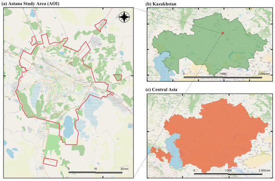
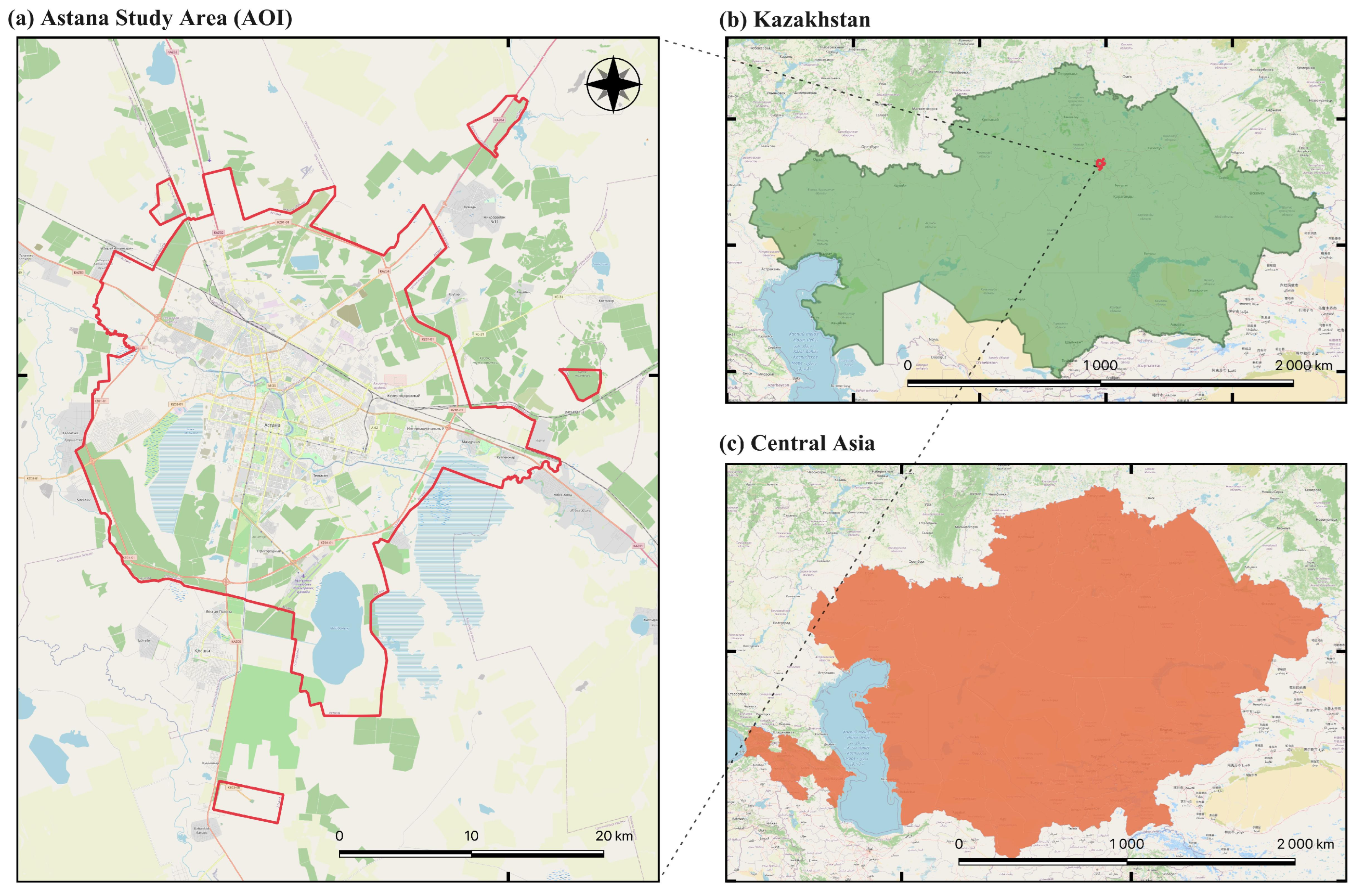


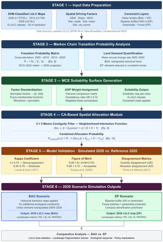
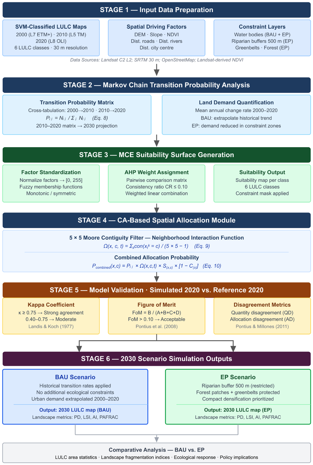
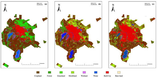
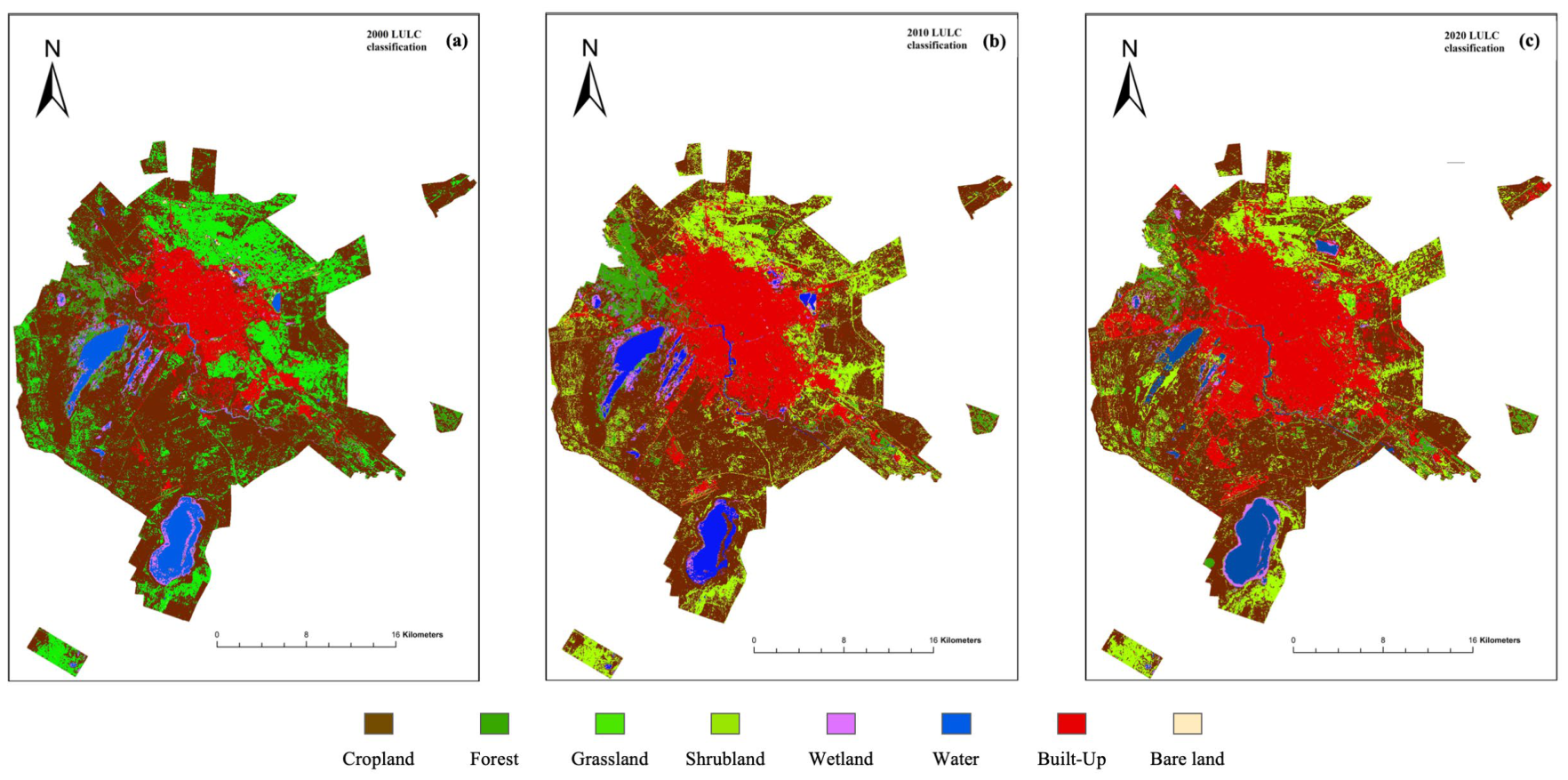
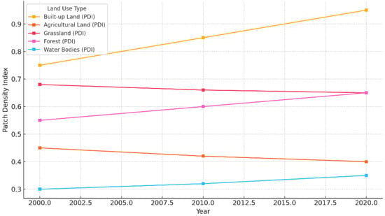
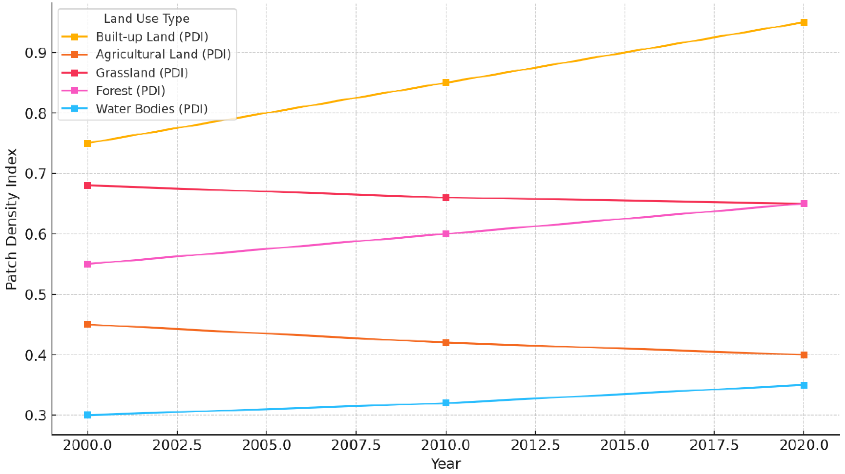
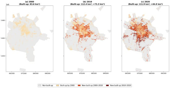
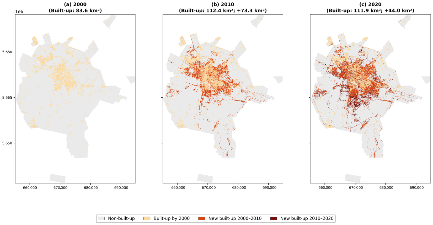
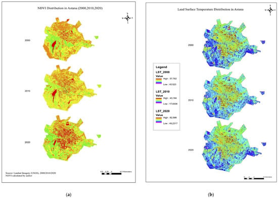
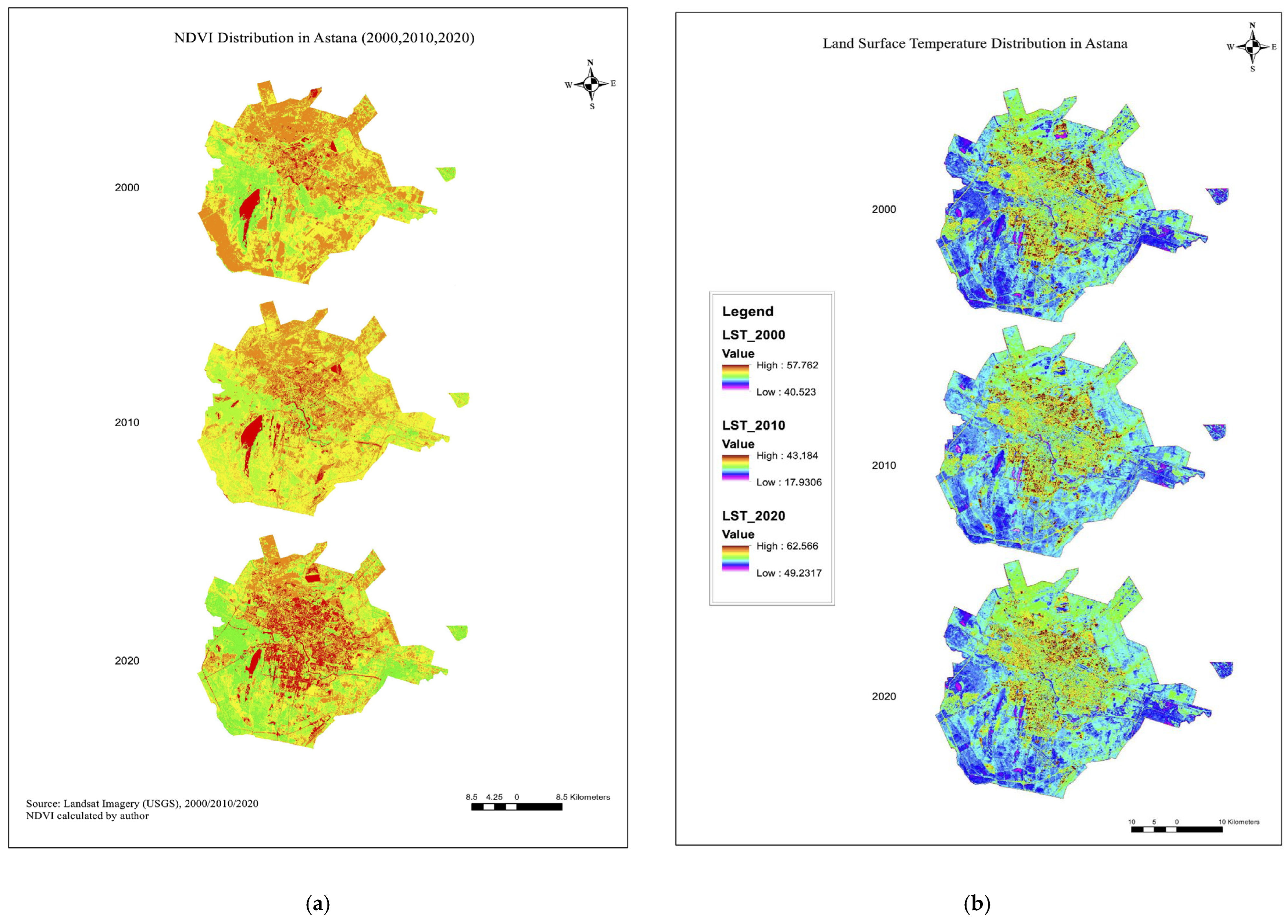
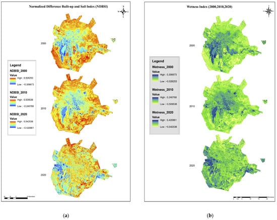
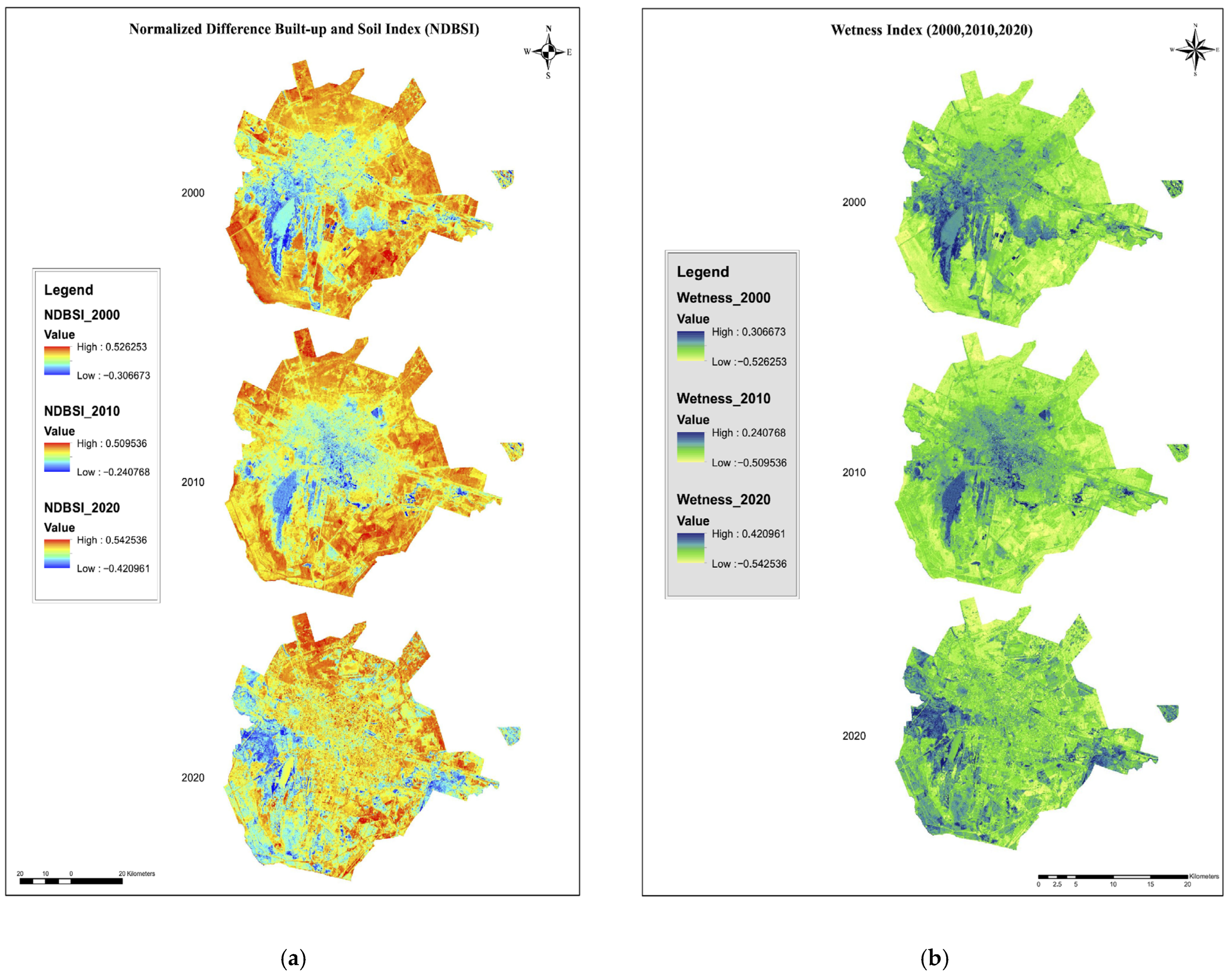
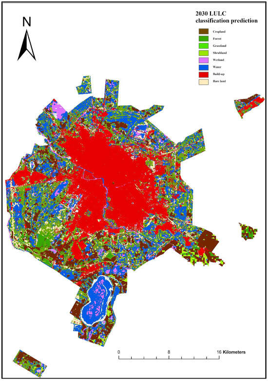
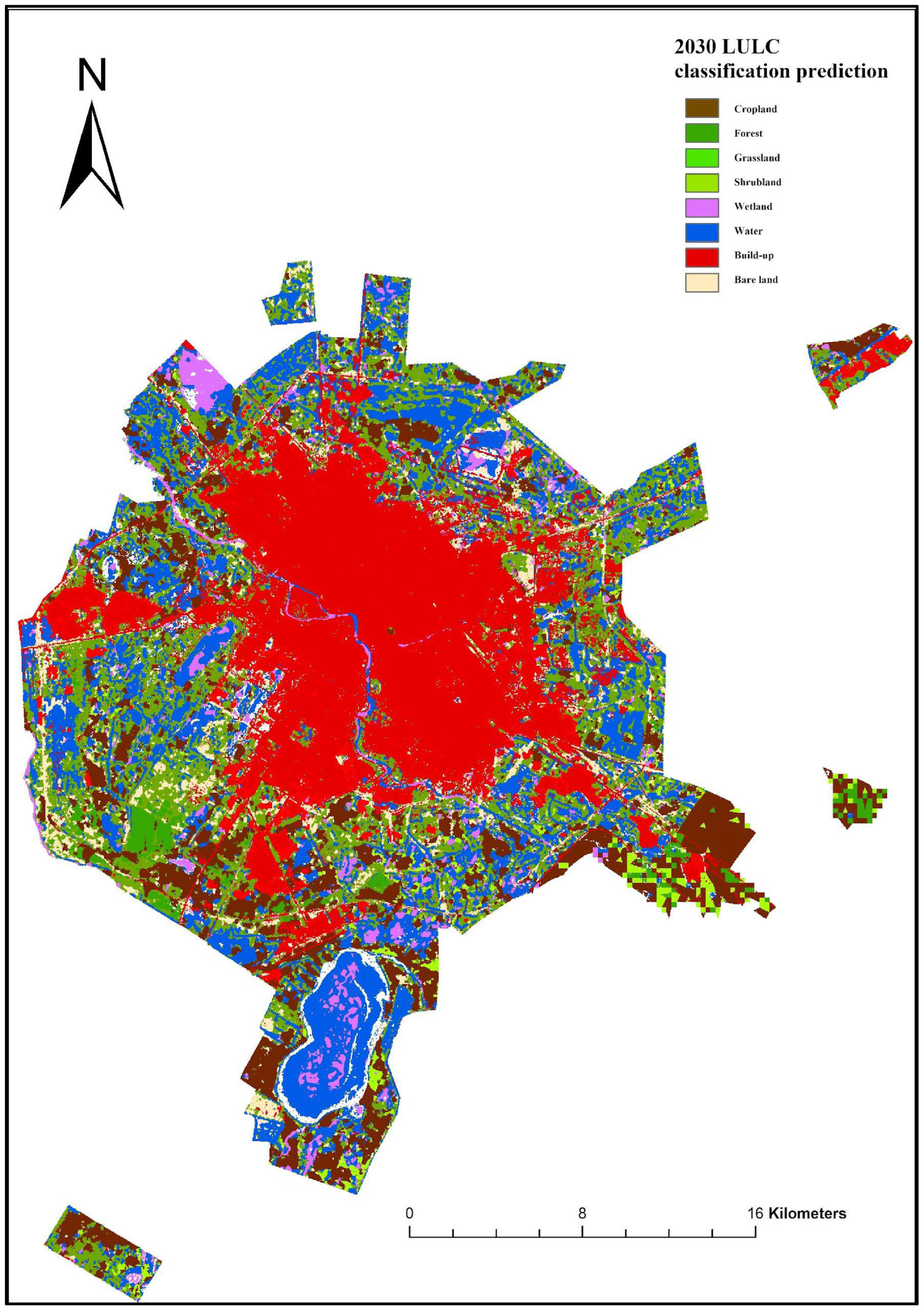

Disclaimer/Publisher’s Note: The statements, opinions and data contained in all publications are solely those of the individual author(s) and contributor(s) and not of MDPI and/or the editor(s). MDPI and/or the editor(s) disclaim responsibility for any injury to people or property resulting from any ideas, methods, instructions or products referred to in the content. |
© 2026 by the authors. Licensee MDPI, Basel, Switzerland. This article is an open access article distributed under the terms and conditions of the Creative Commons Attribution (CC BY) license.