


Abstract
Sustainable air-quality governance requires not only local emission reduction but also a shift from single-pollutant control to coordinated PM2.5–O3 control, and from city-bounded management to regional governance under spatial spillovers. Based on balanced annual city-level panel data for the “2 + 26” urban agglomeration in the Beijing–Tianjin–Hebei region and surrounding areas from 2013 to 2020, this paper uses the dynamic Spatial Durbin Model (SDM) to analyze the spatial spillover effect of PM2.5 and O3 pollution and the effect of regional governance policies. The results show that both PM2.5 and O3 exhibit significant spatial autocorrelation and cross-city dependence, indicating that isolated local control measures are insufficient for sustainable air pollution prevention and that city-bounded governance cannot fully address regionally connected pollution risks. Economic output and secondary-industry employment remain important structural factors of pollution. The policy-text analysis shows that measures centered on coal-related control and industrial governance were more directly aligned with PM2.5 reduction, whereas O3-related governance lagged, suggesting that single-pollutant-oriented control may generate a sustainability trade-off when PM2.5 reduction is not accompanied by coordinated O3 control. These findings highlight two sustainability challenges in China’s regional air-quality governance: first, single-pollutant control can improve particulate pollution but may not ensure sustainable air-quality improvement when O3 and its precursors are insufficiently addressed; second, isolated city-level governance may be insufficient when pollution outcomes exhibit significant spatial dependence across administrative boundaries. The study provides empirical evidence for sustainable air-quality governance by emphasizing differentiated PM2.5 and O3 responses, coordinated PM2.5–O3 control, regional governance beyond individual city boundaries, and the integration of spatial spillover assessment into regional environmental policy design.
1. Introduction
China’s air pollution situation has remained complex, particularly in the Beijing–Tianjin–Hebei region and its surrounding areas. Although fine particulate matter (PM2.5) pollution has improved under strict control measures, ozone (O3) pollution has become increasingly prominent, making coordinated PM2.5 and O3 control a major challenge for regional air-quality governance. Nationwide monitoring data from 2013 to 2020 show that the national average PM2.5 concentration decreased by nearly 48%, but summer O3 concentration increased by about 17%, and in some areas, O3 has replaced PM2.5 as the main pollutant [1,2,3,4]. This contrasting trend reveals a key sustainability problem: improvement in a single pollutant does not necessarily indicate sustainable air-quality governance. A governance framework that reduces PM2.5 but fails to control O3 remains incomplete from a multi-pollutant perspective. This study, therefore, examines PM2.5 and O3 as two policy-relevant outcome indicators for assessing whether regional air-quality governance has moved beyond single-pollutant control toward coordinated multi-pollutant management.
Air pollution also exhibits cross-regional interdependence and spatial spillover effects. Pollution outcomes in one city may be associated with those in neighboring cities because of shared emission sources, regional meteorological conditions, industrial linkages, and coordinated economic activities. This spatial feature creates a second sustainability problem: city-bounded governance may be insufficient when pollution outcomes are connected across administrative boundaries. Since 2013, China has implemented a series of regional joint prevention and control policies, including the Air Pollution Prevention and Control Action Plan, the “2 + 26” Urban Strengthening Program, and the Three-Year Action Plan for Winning the Blue Sky Defense War [5,6]. These policies provide an important context for examining whether regional air-quality governance can generate sustained improvement across both pollutant and spatial dimensions.
Existing studies provide important foundations but leave several gaps. Research on air pollution spillovers has identified spatial autocorrelation, regional clustering, and inter-city dependence using methods such as Moran’s I, spatial panel models, geographically weighted regression, and dynamic spatial econometric models [7,8,9,10,11,12,13,14]. However, many studies treat spatial dependence mainly as a distributional or statistical feature, with less attention to its implications for the sustainability of city-bounded governance. Policy evaluation studies have examined the effects of air-governance interventions using difference-in-differences (DID), spatial DID, synthetic control, and related quasi-experimental approaches [10,11]. These studies improve causal interpretation but often focus on local or single-pollutant outcomes. A growing literature on coordinated PM2.5-O3 control emphasizes the need to address particulate and photochemical pollution together, but it is often more concerned with atmospheric chemistry, exposure risks, or emission-control pathways than with the regional governance implications of differentiated PM2.5 and O3 responses.
This study addresses these gaps by examining PM2.5 and O3 outcomes in the “2 + 26” urban agglomeration under China’s regional air-control policy framework based on the dynamic Spatial Durbin Model (SDM). Specifically, it analyzes the temporal evolution and spatial dependence of PM2.5 and O3, evaluates how pollution outcomes are associated across neighboring cities, and explores how regional governance priorities are related to the differentiated patterns of the two pollutants. This design corresponds to two sustainability concerns: whether single-pollutant governance is sufficient when PM2.5 and O3 respond differently, and whether city-level governance is sufficient when pollution outcomes exhibit inter-city dependence. To complement the econometric analysis, this study also conducts policy-text mining of environmental governance documents from the “2 + 26” cities during 2013–2020. By combining dynamic spatial econometric analysis with policy-text evidence, this study links differentiated PM2.5 and O3 outcomes to the evolution of regional governance priorities in the “2 + 26” urban agglomeration.
In summary, this paper evaluates differentiated PM2.5 and O3 outcomes and their spatial dependence under China’s regional air-control policies. Its marginal contribution is to frame sustainable regional air-quality governance as a dual governance-mismatch problem: the mismatch between PM2.5-oriented policy priorities and the more complex control requirements of O3, and the mismatch between city-bounded governance and inter-city dependence in pollution outcomes. This framework links three strands of literature that are often treated separately: coordinated PM2.5–O3 control, spatial econometric analysis of pollution spillovers, and air-governance policy evaluation. Compared with existing studies, this study emphasizes the governance implications of asymmetric PM2.5 and O3 responses, interprets spatial dependence as a sustainability challenge for city-bounded governance, and uses policy-text analysis to contextualize why PM2.5-centered governance priorities may leave O3 mitigation comparatively delayed. Because the analysis is based on annual city-level panel data, the estimated dynamic and spatial effects are interpreted as evidence of long-term structural persistence and inter-city statistical dependence rather than direct evidence of short-term atmospheric transport or physical pollution propagation.
2. Literature Review
2.1. Research on the Spatial Spillover of Air Pollution
A large body of research has shown that air pollution exhibits spatial correlation and spillover characteristics [12,13,14]. Spatial econometric theory provides the methodological basis for modeling such interdependence. In particular, the Spatial Durbin Model (SDM) can incorporate spatially lagged dependent and explanatory variables, making it suitable for examining both local associations and neighboring-city influences [12,13,15,16]. Empirical studies have used Moran’s I, geographic detectors, multi-scale geographically weighted regression (MGWR), geographically and temporally weighted regression (GTWR), and related spatial methods to identify spatial clustering, heterogeneity, and drivers of PM2.5 or O3 pollution [17,18,19,20]. These studies confirm that air pollution is not randomly distributed across space and that regional interaction should be considered in air-quality analysis.
Recent engineering-oriented studies further emphasize high-resolution monitoring and spatial reconstruction of urban air pollution. For example, Lotrecchiano et al. compared inverse distance weighting with isoelliptical interpolation methods using mobile pollution sensor data from a dynamic road network [21]. Such approaches are useful for reconstructing fine-scale pollution surfaces, incorporating wind-related information, and identifying local pollution hotspots. The present study is complementary to this line of research. Engineering interpolation models help describe where pollution is concentrated at fine spatial and temporal scales, whereas the dynamic SDM used here focuses on long-term inter-city dependence and policy-stage associations at the city-year scale. However, many spatial studies still focus mainly on describing spatial patterns or pollutant drivers, while paying less attention to how spatial dependence challenges the sustainability of city-bounded governance.
2.2. Evaluation Methods of Air-Governance Policies
Environmental policy evaluation studies have increasingly used quasi-experimental methods to estimate the effects of air-governance interventions. Difference-in-differences (DID), spatial DID, synthetic control, and related approaches have been used to examine whether regional policies improved air quality and reduced major pollutants such as PM2.5 in the “2 + 26” cities [22,23,24,25,26,27,28,29]. These studies strengthen causal interpretation by comparing treated and untreated areas or pre- and post-policy changes. Spatial DID studies further show that regional joint prevention and control may generate benefits beyond individual cities when inter-city interaction is considered [25,26,27]. At the same time, environmental regulation may also produce spillover-related risks, including industrial transfer, pollution leakage, or pollution rebound in neighboring areas [26,28]. This literature demonstrates the importance of incorporating a spatial perspective into policy evaluation. Nevertheless, many policy evaluation studies still focus on average local effects or single-pollutant outcomes, and they less often examine how policy priorities are related to differentiated PM2.5 and O3 responses under regional governance.
2.3. Research on Coordinated PM2.5–O3 Control
A growing body of atmospheric environment research emphasizes the need for coordinated PM2.5–O3 control [30,31,32]. Although PM2.5 and O3 differ in formation pathways, they are connected through shared precursors, especially nitrogen oxides (NOx) and volatile organic compounds (VOCs), and through complex atmospheric processes [33,34]. Recent evidence shows that PM2.5 concentrations have declined substantially in China, while O3 pollution has persisted or increased in many regions [3,4,11,31,35,36]. This divergence suggests that single-pollutant control may be insufficient for sustained air-quality improvement. Existing studies therefore call for multi-pollutant strategies, including coordinated VOCs and NOx reduction, precursor-sensitive control, and differentiated measures for particulate and photochemical pollution [31,32,33,34,35,36,37]. However, much of this literature focuses on atmospheric chemistry, exposure risks, or emission-control pathways. Fewer studies connect coordinated PM2.5–O3 control with inter-city spatial dependence and the evolution of regional governance priorities.
Taken together, existing studies provide important but fragmented insights. Spatial econometric studies identify inter-city dependence, policy evaluation studies assess governance interventions, and coordinated-control studies clarify the need to address PM2.5 and O3 together. The present study integrates these strands by examining differentiated PM2.5 and O3 outcomes, spatial spillover-related associations, and policy-priority evolution in the “2 + 26” urban agglomeration. This integrated perspective helps evaluate whether regional air-quality governance can move beyond single-pollutant control and city-bounded management toward coordinated multi-pollutant and cross-city governance.
3. Methods
3.1. Moran’s Index
Before applying spatial econometric models, we first examine whether the data exhibit spatial autocorrelation. If spatial autocorrelation is present, spatial econometric models based on Tobler’s First Law of Geography can be appropriately employed [38,39,40]. Unlike temporal autocorrelation, which occurs only along the time axis, spatial autocorrelation may occur across more directions and can also have an impact on itself.
A positive Moran’s I value indicates positive spatial autocorrelation, meaning that similar values tend to cluster in space. A negative value indicates negative spatial autocorrelation, suggesting that dissimilar values, such as high and low pollution levels, tend to be located near each other. A value close to zero implies a random spatial distribution. Moran’s I is calculated as follows:
n is the total number of spatial units; and represent the observed variables for regions i and j, respectively; is the arithmetic mean of all observations; refers to the spatial weight matrix; and is the sample variance (denoted as ), used to standardize the spatial covariance.
3.2. Spatial Durbin Panel Regression
Spatial autoregressive models mainly include the Spatial Lag Model (SLM), the Spatial Error Model (SEM), and the Spatial Durbin Model (SDM) [16]. The core assumption of the SLM is that the dependent variable (e.g., pollution level in a given region) is influenced by the same variable in neighboring regions (e.g., pollution in nearby cities), thereby exhibiting a “spatial clustering effect”. It captures only the spatial lag of the dependent variable, similar to temporal lag models.
The SEM, by contrast, assumes that spatial dependence exists in the error term rather than among the observed variables themselves. That is, although there may be no spatial interaction among the variables in the model, the unobservable random shocks (residuals), potentially due to omitted variables not included in X but influencing Y, are spatially autocorrelated.
The SDM takes into account both the spatial dependence of the dependent variable and the spatial lags of the independent variables in neighboring regions. As such, the SDM is suitable for examining spatial dependence and indirect associations among neighboring regions when spatial interaction is theoretically expected. Therefore, this study adopts the Spatial Durbin Model as the spatial econometric framework.
In this study, the spatial lag is introduced to capture cross-city dependence in pollution outcomes, while the temporal lag is included to reflect the persistence and delayed adjustment of pollution under evolving economic activity, industrial structure, and policy intervention. Together, these two dimensions make the dynamic SDM more suitable than a static specification for describing the spatiotemporal evolution of PM2.5 and O3.
3.2.1. Model Specification Tests
To determine the appropriate spatial econometric specification, we first conducted Lagrange Multiplier (LM) tests and robust LM tests based on the baseline OLS model for both PM2.5 and O3. In Table 1, for PM2.5, the LM–error statistic was 222.660 (p < 0.001), the LM–lag statistic was 37.507 (p < 0.001), the robust LM–error statistic was 192.145 (p < 0.001), and the robust LM–lag statistic was 6.993 (p = 0.008). For O3, the LM–error statistic was 50.846 (p < 0.001), the LM–lag statistic was 37.539 (p < 0.001), the robust LM–error statistic was 27.724 (p < 0.001), and the robust LM–lag statistic was 14.417 (p < 0.001). These results indicate significant spatial dependence in both the lag term and the error term, suggesting that non-spatial OLS is inadequate and that a spatial econometric framework is required [41].
Table 1.
Specification tests for selecting the spatial econometric model.
We then compared the goodness of fit of alternative spatial models. For PM2.5, the log-likelihood values were −981.950 for OLS, −962.077 for the Spatial Lag Model (SLM), −808.034 for the Spatial Error Model (SEM), and −717.054 for the Spatial Durbin Model (SDM). For O3, the corresponding values were −230.186, −210.747, −199.674, and −130.024, respectively. In both cases, the SDM yielded the highest log-likelihood, indicating the best model fit among the competing specifications.
In addition, likelihood ratio (LR) tests further supported the SDM specification. For PM2.5, the LR statistics were 39.745 (OLS vs. SLM, p < 0.001), 529.792 (OLS vs. SDM, p < 0.001), and 490.046 (SLM vs. SDM, p < 0.001). For O3, the corresponding LR statistics were 38.878 (p < 0.001), 200.324 (p < 0.001), and 161.446 (p < 0.001). Taken together, the LM diagnostics, the likelihood comparisons, and the LR tests indicate that the SDM provides a more appropriate specification than the OLS, SLM, and SEM for the present study. Therefore, the dynamic SDM was retained for the subsequent analysis.
3.2.2. Spatial Weights
To quantify spatial weights among different spatial units, we employ the K-nearest neighbors (KNNs) spatial weight matrix (k = 10) as the benchmark specification for the measurement of geographic weighting of SDM [42,43]. In constructing the weights, the geographical coordinates (latitude and longitude) of each minimal observation unit are used to calculate the Euclidean distances to all other points. The K-nearest neighbors are then selected as the spatially connected entities. Specifically, if city j is among the K-nearest neighbors of city i, ; otherwise, . Under this setting, each city maintains a fixed number of spatial connections, which helps avoid isolated observations and improves comparability in an irregularly distributed city-level panel. This feature is especially useful in the present study, where the analysis concerns not only inter-city spatial dependence but also relatively stable inter-city interactions under the “2 + 26” regional governance framework [42]. This method ensures that each observation maintains a fixed and sufficient number of spatial connections, thereby enhancing the connectivity and density of the spatial weight matrix.
To ensure comparability of spatial weights, the KNN spatial weight matrix is further row-standardized, such that the sum of neighbor weights for each spatial unit equals one. This construction improves comparability across cities and supports subsequent tests of spatial autocorrelation and spatial econometric estimation. At the same time, we acknowledge that alternative matrices, especially inverse-distance matrices, are also widely used in air pollution research because they can more directly reflect how spatial dependence and inter-city association tend to weaken as geographic distance increases. Therefore, the KNN matrix in this study should be understood as the benchmark specification for capturing stable neighborhood dependence, whereas alternative distance-based matrices provide an important robustness direction. As an additional robustness exercise, we also tested a row-standardized inverse-distance specification. The inverse-distance spatiotemporal matrix was successfully constructed on the same sample, and the corresponding spatial lag variables were generated successfully. Although the fully specified inverse-distance ML–Lag estimation was computationally not stable enough in the current environment, the diagnostic evidence and qualitative pattern were broadly consistent with the benchmark KNN specification. The robustness results based on alternative KNN settings and the inverse-distance matrix are reported in Section 5.1.5 and Section 5.1.6, which help assess whether the main spatial-dependence findings are sensitive to the choice of spatial weight matrix.
3.2.3. Variable Selection
Our variables are based on the Environmental Kuznets Curve (EKC), relevant Chinese air-governance policies, and the IPAT/STIRPAT framework [44,45,46]. The EKC is widely used to describe the relationship between economic development and environmental pollution. As the economy grows, environmental degradation is often observed to follow an inverted U-shaped trajectory. Empirical studies on the EKC suggest that effective environmental regulations can shift the EKC turning point and support pollution control without hindering economic growth [46].
The IPAT equation, proposed by Ehrlich and Holdren, posits that environmental impact (I) is determined by population (P), affluence (A), and technology (T) [44]. The IPAT framework and its extensions, such as STIRPAT, have been widely applied to quantify the drivers of environmental pressure, and recent panel-data applications further improve its econometric use [45]. In this study, the IPAT framework is used as a heuristic reference rather than a strict one-to-one operationalization. Accordingly, the selected variables are interpreted as structural proxies for the three dimensions of IPAT under the regional governance context of the “2 + 26” urban agglomeration. In particular, the P dimension is approximated by employment in the primary, secondary, and tertiary sectors, which is intended to capture the scale and allocation of labor-related human activity rather than literal demographic population; regional GDP and per capita GDP are used to capture affluence (A); and the number of newly registered high-tech enterprises is used as a proxy for technology and innovation capacity (T). .
3.2.4. Variables Measurement
In the dynamic SDM model,
The dependent variable denotes both and , : logarithm of O3, and : Moran index concentration in city i during year t (dependent variable); : time lag term, which is conveyed by delta_moran, showing the change from the previous year; : spatiotemporal lag of the dependent variable, i.e., the spatially weighted (neighboring cities) lagged term is W_ln_PM2.5; : independent variables (covariates related to economy, enterprises, innovation, environmental protection, that is, ln_PICo_new, etc.); : spatially lagged independent variables (W_ln_PICo_new, etc.); : province fixed effects; : year fixed effects (post_2017, etc.); : error term; : parameters to be estimated; and : elements of the spatial weight matrix [15,16].
The independent variables include: .
- Population (P)
- : Natural logarithm of employment in the primary industry (scale of agriculture); : natural logarithm of employment in the secondary industry (labor input in industry and manufacturing); : natural logarithm of employment in the tertiary industry (human resources in the service sector).
- 2.
- Affluence (A)
- ln_Grorgdpput: Natural logarithm of Gross Regional Product (total economic output).
- ln_GDPgwrate: GDP growth rate (annual economic growth, reflecting economic dynamism).
- 3.
- Technology (T)
- : Natural logarithm of the number of newly registered pollution-intensive enterprises.
- : Natural logarithm of the total number of pollution-intensive enterprises (stock of industrial market actors).
- : Natural logarithm of the total number of high-tech enterprises (stock of innovation-oriented entities).
- 4.
- Policy Dummy Variables
- : Policy dummy variables (2017 marks the final phase of the “Ten Measures for Air”; 2020 corresponds to the peak of the “Blue Sky Protection Campaign”).
- 5.
- Dynamic Effects of Environmental Pollution
- : First-order lag of PM2.5 concentration (temporal inertia of pollution).
- : Spatially weighted average of PM2.5 concentration in neighboring cities (spatial spillover effect).
This study constructs the spatial weight matrix using the K-nearest neighbors (KNNs) method to ensure that spatial correlation aligns with geographic proximity. All logarithmic variables have been adjusted to account for zero values. The above variables comprehensively cover the three main components of the IPAT model—population, affluence, and technology—as they relate to environmental pollution, while also incorporating policy factors, which are a central focus of the later analysis. Together, these variables provide structural proxies for examining how socioeconomic conditions, enterprise structure, innovation capacity, and policy stages are associated with regional pollution outcomes and spatial-dependence patterns.
The dependent variables are the natural logarithms of annual average PM2.5 concentrations and ozone-season mean MDA8 O3 concentrations. Specifically, O3 is measured as the mean of daily maximum 8 h average O3 concentrations during the high-ozone season from April to October. The independent variables include employment figures in the primary, secondary, and tertiary sectors as proxies for labor-related economic activity and industrial structure, rather than direct measures of population exposure; GDP and GDP growth are used to capture economic development; and the number of high-tech enterprises is used as a proxy for technological and innovation capacity. Dummy variables for the policy stages 2017 and 2020 are introduced to reflect two major rounds of national air–governance intervention. Specifically, post_2017 is coded as 1 for the years 2017–2020 and 0 otherwise, capturing the strengthened governance stage associated with the concluding phase of the national “Air Pollution Prevention and Control Action Plan” and the intensified control of the “2 + 26” cities. Post_2020 is coded as 1 for the year 2020 and 0 otherwise, capturing the latter policy stage represented by the height of the “Blue Sky Protection Campaign”. These policy-stage dummy variables enter the model directly to reflect common time-specific governance shocks, whereas spatial lag terms are constructed only for the main continuous explanatory variables.
3.3. Study Area and Data
The study area in Figure 1 covers the Beijing–Tianjin–Hebei region and its surrounding “2 + 26” cities, including cities in Beijing, Tianjin, Hebei, Shanxi, Shandong, Henan, and neighboring areas. This region is one of China’s key areas for regional joint prevention and control of air pollution and is characterized by dense industrial activities, frequent cross-city pollutant transport, and strong policy relevance. Figure 1 shows the geographical location of the study area and the spatial distribution of the “2 + 26” cities.
Figure 1.
Location of the study area. The left panels show the location of the Beijing–Tianjin–Hebei region and surrounding provinces within China, and the right panel shows the spatial distribution of the “2 + 26” cities included in this study.
In this study, observed hourly PM2.5 and O3 concentrations at national monitoring stations during 2013 to 2020 were obtained from the National Air Quality Real-Time Publishing Platform maintained by the China National Environmental Monitoring Center (https://air.cnemc.cn:18007/, accessed on 26 August 2025) [47]. Socioeconomic indicators at the city level, including GDP, sectoral employment, enterprise counts, and other relevant variables, were obtained from the China Research Data Services Platform (https://www.cnrds.com/, accessed on 26 August 2025) [48]. All variables are aggregated into annual prefecture-level data to form a city-level panel dataset covering 2013–2020, rather than a single-year cross-sectional dataset, and transformed using natural logarithms to mitigate scale differences. Specifically, hourly PM2.5 and O3 observations from national monitoring stations are first aggregated to the prefecture-level city unit. For descriptive analysis, these data are further summarized at the monthly city level to illustrate seasonal variation, whereas for the benchmark regression, PM2.5 observations are aggregated into annual city-level averages, and O3 observations are first converted into daily maximum 8 h average values and then averaged over April–October to obtain city-year ozone-season MDA8 O3 indicators.
Therefore, the dependent variables in the SDM are the natural logarithms of annual prefecture-level PM2.5 concentrations and prefecture-level ozone-season mean MDA8 O3 concentrations, rather than monthly or station-level observations. Missing values are supplemented using linear interpolation. More specifically, linear interpolation was applied only to limited intermittent missing observations after the annual city-level aggregation in order to preserve panel continuity. In addition, the pollution indicators are derived from monitoring observations aggregated from station level to the prefecture-level city unit, which may still contain residual measurement heterogeneity across cities and years. Therefore, the empirical results should be interpreted with appropriate caution as evidence on broad spatiotemporal patterns and structural associations, rather than as noise–free measurements of all determinants of pollution. Detailed definitions, aggregation rules, and data sources of the main variables are reported in Supplementary Table S6.
To account for inflation, price-related indicators are adjusted using the GDP deflator to reflect constant prices based on the year 2013. The study period was limited to 2013–2020 because 2013 marks the launch of the national “Air Pollution Prevention and Control Action Plan”, while 2020 represents the end of a relatively complete policy stage examined in this study, thus providing a consistent time window for evaluating pollution dynamics and policy effects. We acknowledge that meteorological conditions are important determinants of both PM2.5 and O3, especially for pollutant dispersion and ozone formation. Because the present analysis is based on annual city-level panel data and focuses on long-term socioeconomic structure, policy-stage associations, and inter-city spatial dependence, the benchmark model prioritizes structural and policy-related variables within a unified regional panel. This specification does not imply that meteorology is unimportant; rather, the estimated coefficients should be interpreted as long-term structural associations under the observed governance context, not as a complete causal decomposition of short-term atmospheric processes. To address the potential influence of omitted meteorological conditions, we further conduct a robustness check by adding annual precipitation, sunshine hours, and annual mean temperature as city-year meteorological controls (Supplementary Table S4). The supplementary results show that the main spatial-dependence findings remain robust after controlling for broad annual meteorological conditions.
3.4. Supplementary Identification Strategies
To further alleviate endogeneity concerns while preserving the benchmark spatial framework, this study supplements the dynamic SDM with three quasi-experimental identification strategies: a two-way fixed-effects DID design, a matched DID/event-study design, and a spatial exposure DID with placebo tests.
First, the baseline DID compares the original “2 + 26” cities with all non-treated prefecture-level cities in the broader city panel over the period of 2013–2021, where 2013–2016 is defined as the pre-policy period and 2017–2021 as the post-policy period. City fixed effects and year fixed effects are included to remove time-invariant city heterogeneity and common annual shocks.
Second, to improve pre-policy comparability, a matched DID and event-study design is implemented. Matching is conducted on the basis of pre-policy average pollution levels, pre-policy pollution trends, geographic coordinates, and major socioeconomic characteristics. The donor pool is first restricted by geographic proximity to the “2 + 26” area, and then nearest-neighbor matching with caliper restrictions is applied to construct a more comparable treated–control sample.
Third, to further examine spatial externalities, a spatial exposure DID is estimated for non-treated cities only. In this specification, exposure to the policy core area is measured by the distance to the nearest “2 + 26” city. Both binary exposure and continuous exposure specifications are considered, with the latter defined as the inverse distance and alternative spatial weight matrices to the nearest treated city interacted with the post-policy period. Finally, placebo tests using false policy years are conducted to assess whether the estimated post-policy patterns are likely to reflect genuine policy-related changes rather than pre-existing spurious trends.
4. Results
4.1. Spatial and Temporal Variations
Figure 2 presents the spatial distribution of ozone-season mean MDA8 O3 (calculated as the April–October mean of daily maximum 8 h average O3 concentrations) and annual average PM2.5 concentrations in China in 2014, 2017, and 2020. The two pollutants display contrasting temporal patterns. O3 concentrations increased from 2014 to 2017 and remained relatively high in 2020. Spatially, high O3 concentrations are mainly distributed in northern China, including the Beijing–Tianjin–Hebei region, Shandong, Shanxi, Liaoning, and Henan, as well as in the Yangtze River Delta. By contrast, lower O3 concentrations are more common in western and southwestern regions, including Xinjiang, Qinghai, Tibet, Yunnan, Guizhou, and Guangxi. This spatial pattern may be associated with regional differences in economic activity, industrial structure, precursor emissions, and meteorological conditions.
Figure 2.
The spatial distribution of ozone-season mean MDA8 O3 (μg/m3) and annual mean PM2.5 (μg/m3) concentrations in China in 2014, 2017, and 2020. Rectangles refer to the observation sits in the “2 + 26” region.
On the other hand, PM2.5 shows a clear downward trend. High PM2.5 concentrations were widespread in 2014, especially in central and eastern China, but declined markedly by 2017 and further by 2020. The reduction is particularly evident in the Beijing–Tianjin–Hebei region and surrounding areas, although some central and northern cities still maintain relatively higher PM2.5 levels than western and southern regions. This contrast between rising or persistent O3 and declining PM2.5 indicates that particulate-pollution improvement has not been accompanied by equivalent O3 mitigation.
Supplementary Figure S2 further illustrates the seasonal variation in PM2.5 and O3 in selected years. PM2.5 shows a typical winter-high and summer-low pattern, whereas O3 exhibits the opposite seasonal pattern, with higher concentrations in late spring and summer. These monthly patterns are reported as descriptive background only. They are not used as direct inputs in the SDM regression, which is estimated using annual city-level panel data because the socioeconomic indicators and policy-stage variables are defined at the yearly level.
4.2. Exploratory Spatial Data Analysis
4.2.1. Autocorrelation Analysis
As shown in Figure 3, both PM2.5 and O3 exhibited significant positive spatial autocorrelation in 2014, 2017, and 2020. For PM2.5, Moran’s I increased from 0.395 in 2014 to 0.625 in 2017 and further to 0.715 in 2020, with p-values equal to 0.0000 in all three years. This indicates that PM2.5 pollution became increasingly clustered over time, and that areas with relatively high or low PM2.5 concentrations tended to be located near areas with similar pollution levels. Compared with PM2.5, O3 showed stronger spatial dependence in 2017 and 2020. Overall, both pollutants were characterized by significant and persistent spatial clustering, while the spatial autocorrelation of O3 strengthened more markedly over time. Because this exploratory spatial analysis is based on annual city-level pollution data, these Moran’s I results should be interpreted as descriptive evidence of annual spatial association and regional clustering, rather than as direct evidence of short-term atmospheric transport or a complete physical propagation mechanism.
Figure 3.
Spatial correlation of O3 and PM2.5 in 2014, 2017, and 2020. The x-axis represents normalized concentration and the y-axis represents normalized spatial lag.
4.2.2. Policy Analysis
Policy evolution in the “2 + 26” urban agglomeration reflects two sustainability challenges: the shift from single-pollutant control to coordinated PM2.5–O3 control, and the shift from city-bounded regulation to regional governance under spatial spillovers. Since the 2013 Air Pollution Prevention and Control Action Plan, the “2 + 26” cities have served as a strategic core area of China’s regional joint prevention and control policies. Early policy measures emphasized coal control, industrial-emission reduction, and PM2.5 mitigation, while later measures, including the strengthened governance of the “2 + 26” cities and the Blue Sky Defense Campaign, further reinforced regional coordination.
During 2013–2020, PM2.5 declined substantially in the “2 + 26” cities, whereas O3 remained high or continued to increase in some areas. This divergence suggests that PM2.5-oriented policy priorities were more directly aligned with particulate-pollution reduction, while systematic O3-oriented governance, especially VOCs–NOx coordination and precursor-sensitive control, entered the policy agenda more gradually. The observed pattern, therefore, illustrates a key limitation of single-pollutant-oriented governance: improvement in PM2.5 does not necessarily imply parallel progress in O3 mitigation. These policy-stage patterns provide the governance context for interpreting differentiated PM2.5 and O3 outcomes under regional interdependence. Because the analysis is based on annual city-level panel data, the results capture broad policy-stage associations and long-term inter-city dependence, rather than short-term atmospheric chemistry, meteorological variability, or specific pollution-episode mechanisms.
4.2.3. Interpretation of Local Indicators of Spatial Association (LISA) Results
As shown in Figure 3, Moran scatter plots divide each spatial unit into four quadrants, representing high–high clusters (first quadrant), low–high clusters (second quadrant), high–low clusters (fourth quadrant), and low–low clusters (third quadrant). During the 2013–2020 period, the vast majority of O3 monitoring sites were distributed in the first and third quadrants, which means that positive spatial autocorrelation is prevalent between spatial units: high pollution areas are clustered. Geographical visualization further confirms this spatial agglomeration feature. The high–high cluster is mainly distributed in northern China and the Yangtze River Delta, reflecting the ozone pollution pressure in regions with a developed economy, high energy consumption, and high motor vehicle ownership. However, the low–low cluster is mainly concentrated in the lower population density regions in the northeast, northwest, and southwest of China, which may benefit from the clean energy mix and lower urbanization level. Because the LISA analysis is descriptive, these clusters should be interpreted as annual spatial association patterns rather than as a complete explanation of ozone formation.
Figure 4 further illustrates the spatial distribution of Local Moran’s I for O3 and PM2.5 in 2014, 2017, and 2020. The local spatial association of O3 was mainly concentrated in northern China, the Beijing–Tianjin–Hebei region, and parts of the Yangtze River Delta, where higher Local Moran’s I values indicate stronger local clustering of ozone pollution. Although PM2.5 also showed positive local clustering, its spatial pattern appeared somewhat narrower than that of O3, especially in 2017 and 2020. This difference is consistent with the stronger global spatial autocorrelation of O3 shown in Figure 3. Across the selected annual observations from 2014 to 2020, these high-value areas remained relatively stable, and in some places became more concentrated, suggesting persistent regional linkage and dependence of O3 pollution.
Figure 4.
Spatial sistribution of local Moran’s I. (a) Moran Index of Ozone in 2014; (b) Moran Index of Ozone in 2017; (c) Moran Index of Ozone in 2020; (d) Moran Index of PM2.5 in 2014; (e) Moran Index of PM2.5 in 2017; (f) Moran Index of PM2.5 in 2020; Rectangles refer to the observation sits in the “2 + 26” region.
The high-value areas were more spatially concentrated in the Beijing–Tianjin–Hebei region and nearby industrial cities. These local clustering patterns further justify the focus on the “2 + 26” urban agglomeration in this study. As a nationally designated policy core area and a region characterized by notable inter-city association and spatial dependence, the “2 + 26” cities provide a suitable empirical setting for assessing regional governance effectiveness and spatial spillover effects.
5. Regression
5.1. Analysis of Dynamic SDM Results from 2 + 26 Cities
5.1.1. The Main Driving Factors
- Economic development and industrial structure
The regression results in Table 2 and Table 3 show that regional GDP (ln_Grorgdpput) is positively and significantly associated with both PM2.5 and O3 (the coefficients are 0.078 and 0.050, respectively, both p < 0.05). Table 4 and Table 5 report the model summaries and goodness-of-fit statistics for the PM2.5 and O3 dynamic SDM models, respectively, and the relatively high pseudo R-squared values and log-likelihood statistics indicate that both models provide an acceptable fit to the annual city-level panel data.This result suggests that economic expansion is associated with higher pollution pressure under the current development pattern. The EKC conjecture may imply that the pollution-reduction turning point has not yet been clearly reached, but this interpretation remains tentative within the present annual-data framework. In addition, the employment scale of the secondary industry (ln_Scidempnum) is also positively associated with both pollutants (PM2.5: 0.061, p < 0.01; O3: 0.015, p < 0.10). It should be noted that sectoral employment is used here as a proxy for labor-related economic activity and industrial structure, rather than as a direct measure of total population or population exposure. Therefore, its coefficient should be interpreted as an association between the allocation of economic activity and pollution outcomes, not as a demographic effect in a strict sense. Taken together, the positive coefficients of GDP and secondary-industry employment support a cautious structural interpretation: regional growth remains associated, at least in part, with pollution-intensive industrial activities. The coefficient of delta_moran_ PM2.5 is negative, whereas the corresponding coefficient in the O3 model is positive; however, both effects are statistically insignificant. This suggests that short-term changes in local spatial correlation do not show a stable and robust association with the spillover dynamics of the two pollutants in the present model.
Table 2.
Regression results for PM2.5 dynamic SDM.
Table 3.
Regression results for O3 dynamic SDM.
Table 4.
Model summary for PM2.5 dynamic SDM.
Table 5.
Model summary for O3 dynamic SDM.
- 2.
- The stock of polluting enterprises and the entry of new enterprises
In the PM2.5 model, the stock of polluting enterprises (ln_PICo_total) is positively and significantly associated with pollution concentration (0.048, p = 0.048), suggesting that the historically accumulated distribution of polluting enterprises is related to the current spatial differentiation of particulate pollution. The coefficient of newly established polluting enterprises (ln_PICo_new) is also positive and significant (0.036, p = 0.045), indicating that new pollution-intensive enterprise entry is associated with additional PM2.5 pressure (Table 2). For the O3 model, the effect of stock enterprises is negative but statistically insignificant (−0.0136, p = 0.479), suggesting that ozone pollution is less directly linked to the simple stock of polluting firms and cannot be robustly explained by this variable alone. However, the coefficient of newly established polluting enterprises in the O3 model is positive but statistically insignificant (0.023, p = 0.126), suggesting that the relationship between new polluting entrants and ozone formation is more uncertain and may depend more strongly on precursor chemistry and broader atmospheric conditions (Table 3).
- 3.
- High-tech enterprises (industrial upgrading)
The coefficient of the number of high-tech enterprises (ln_HTCo_total) in the PM2.5 model is −0.067 (p < 0.001), suggesting that high-tech enterprise agglomeration is negatively associated with PM2.5 concentration. This pattern is consistent with the interpretation that innovation-oriented industrial upgrading may contribute to particulate-pollution mitigation (Table 2). In the O3 model, the coefficient is also negative (−0.012) but statistically insignificant (p = 0.348), indicating that the effect of high-tech development on ozone mitigation remains limited or uncertain under the current policy and precursor–control framework. Therefore, the present results suggest that high-tech development is more clearly associated with PM2.5 mitigation than with O3 control. In other words, industrial upgrading appears to be more closely related to particulate reduction, whereas its relationship with O3 remains limited or uncertain under the current precursor-control framework. This difference should be interpreted cautiously because O3 is a secondary pollutant formed through nonlinear photochemical reactions involving VOCs and NOx, and because meteorological controls are not included in the benchmark model (Table 3).
- 4.
- Policy Intervention and Differentiated Pollution Responses
The coefficient of the “Air Pollution Prevention and Control Action Plan” policy (post_2017) in the PM2.5 model is significantly negative (−0.108, p < 0.001), suggesting that PM2.5 concentration was lower during the strengthened governance stage after 2017 (Table 2). However, the corresponding policy-stage coefficient in the O3 model is significantly positive (0.046, p < 0.001), suggesting that the strengthened governance stage after 2017 was not accompanied by parallel O3 mitigation. A more appropriate interpretation is that the policy package during this stage was more directly aligned with PM2.5-oriented measures, such as coal-combustion control, industrial regulation, and end-of-pipe treatment, whereas O3 control depends more strongly on coordinated VOCs and NOx reduction, precursor-balance management, photochemical conditions, and meteorological factors. Therefore, the positive O3 coefficient reflects an asymmetric policy-stage association: PM2.5 improved more clearly under the existing governance framework, while O3 mitigation remained comparatively delayed and more difficult. This pattern provides evidence of the sustainability limitation of single-pollutant-oriented governance under coordinated PM2.5–O3 pollution control (Table 3). This asymmetric pattern is consistent with the different formation mechanisms of the two pollutants. PM2.5 includes both primary emissions and secondary components, so policies targeting coal combustion, industrial sources, and end-of-pipe control can often generate relatively direct reductions in particulate pollution. By contrast, O3 is a secondary pollutant formed through nonlinear photochemical reactions involving NOx and VOCs. Its concentration depends not only on precursor emissions, but also on the VOCs–NOx sensitivity regime, solar radiation, temperature, humidity, wind conditions, and boundary-layer dynamics. Therefore, O3 does not necessarily respond to end-of-pipe industrial control or coal-combustion reduction in the same way as PM2.5. Therefore, under the same policy framework, PM2.5 may decline more clearly, whereas O3 can remain difficult to control or even rebound in some cases. This also helps explain why O3-related governance remained comparatively delayed and less targeted than PM2.5 control during the study period.
This result should be interpreted within a phased policy context. Earlier intervention stages mainly targeted coal combustion, industrial emissions, and PM2.5 reduction, whereas O3-related governance entered the policy agenda later and remained less specific. Therefore, the asymmetric coefficients of PM2.5 and O3 should be understood within the path-dependent evolution of China’s staged air-governance framework. Earlier policy stages were more closely connected with particulate-matter control through coal reduction, boiler retrofitting, and industrial regulation, while systematic O3-oriented measures, especially VOCs and NOx coordination, became more visible later in the policy process. In this sense, the coefficients capture differentiated policy-stage associations between governance priorities and pollution outcomes. They help explain why PM2.5 responded more clearly to the existing governance framework, whereas O3 mitigation remained less synchronized and more difficult to achieve.
5.1.2. Model Validity and Goodness of Fit
The goodness-of-fit results are consistent with the model specification tests reported in Section 3.2.1 and further support the use of the SDM in the subsequent analysis. For the PM2.5 model, the Pseudo R-squared is 0.7713, and the spatial lag coefficient is highly significant (ρ = 0.858, p < 0.001), indicating a higher degree of fitting and substantial spatial dependence. For the O3 model, the Pseudo R-squared is 0.8985, and the spatial lag coefficient is also highly significant (ρ = 0.752, p < 0.001), suggesting that spatial interaction remains an important feature of ozone pollution. Overall, these results indicate that the estimated SDM captures major spatial and temporal patterns in both pollutants and provides a statistical basis for interpreting structural associations and inter-city dependence.
5.1.3. Spatial Spillover Effects and Inter-City Dependence Patterns
- Strong spatial autocorrelation
The coefficients of the spatial lag term of the two groups of models are significantly positive: PM2.5 is 0.858, and O3 is 0.752 (both p < 0.001), indicating that the spatial spillover effect of both particulate matter and ozone pollution is highly significant. PM2.5 is particularly prominent, and it provides evidence of strong inter-city dependence and persistent regional association (such as the Beijing–Tianjin–Hebei region and the Fen–Wei Plain) under the background of the “Air Pollution Prevention and Control Action Plan”. The spatial dependence of O3 is also substantial, which is consistent with the regional nature of ozone pollution and its complex coupling with VOCs, NOx, meteorological conditions, and photochemical processes. Because meteorological variables are not included in the benchmark model, the O3 spatial coefficient should be interpreted as a combined long-term regional association rather than a single identifiable transport mechanism. Supplementary Table S4 shows that the main spatial-dependence findings remain robust after adding annual precipitation, sunshine hours, and annual mean temperature.
- 2.
- The importance of joint policy prevention and coordinated emission reduction
The significant inter-city dependence suggests that city-bounded governance may be insufficient for sustainable regional air-quality improvement. Local pollution-control achievements may be fragile if neighboring cities are not governed in a coordinated way. For example, industrial relocation or the gradient transfer of high-energy-consuming industries may reduce pollution pressure in core cities, but may also shift pollution-intensive activity to surrounding areas, creating potential risks of renewed regional pollution pressure. O3 governance requires particular attention to the regional coordination of precursor emissions. If VOCs and NOx emissions are not jointly managed across cities, PM2.5 improvement may not translate into coordinated PM2.5–O3 improvement, and local gains may be weakened by renewed pollution pressure from neighboring areas.
Therefore, it is suggested to promote regional linkage, unified planning, and strengthen the regional coordination mechanism for correcting unintended cross-city pollution effects to achieve coordinated prevention and control of air pollution and maximize its efficiency. More importantly, the present findings also have broader implications for future studies on regional air pollution governance. These results are broadly consistent with previous studies emphasizing the spatial dependence of air pollution and the importance of coordinated regional governance [27,28,29]. However, compared with studies focusing on a single pollutant or using static spatial models [35,36], our results further show that PM2.5 and O3 may respond asymmetrically to the same policy intervention in the “2 + 26” urban agglomeration. This suggests that future studies should pay greater attention to multi-pollutant interactions and phase-specific policy responses. In practical terms, policy design should place greater emphasis on coordinated VOCs and NOx reduction, cross-provincial meteorological early-warning mechanisms, and differentiated governance targets for PM2.5 and O3, rather than relying on a single-pollutant evaluation framework.
5.1.4. Supplementary DID, Spillover DID, and Placebo Evidence
To provide supplementary evidence on policy-stage associations and to examine the limits of city-bounded policy evaluation, we supplemented the benchmark dynamic SDM with a two-way fixed-effects DID design, a spatial exposure DID, and placebo tests. Detailed coefficient estimates are reported in Supplementary Tables S1–S3.
The baseline DID results show that the post-policy interaction term is negative but statistically insignificant for PM2.5 (coef. = −0.0401, p = 0.6408), whereas it is positive and statistically significant for O3 (coef. = 0.1761, p = 0.0267). These estimates suggest that, relative to non-treated cities, the strengthened intervention in the “2 + 26” cities did not generate a clearly identifiable additional reduction in PM2.5, but was associated with a significant relative increase in O3. The insignificant PM2.5 DID coefficient is informative rather than merely inconsistent with the benchmark results. It suggests that PM2.5 reductions during this period were not clearly separable between treated and non-treated cities, possibly because national pollution-reduction trends and inter-city spillover processes crossed the administrative boundary of the “2 + 26” treatment group.
This also implies that the stable unit treatment value assumption (SUTVA) required by conventional DID may be difficult to satisfy in regional air pollution governance. The statistically insignificant PM2.5 DID coefficient should therefore not be treated merely as weak or directionally consistent evidence. Instead, it provides indirect support for the main spatial argument of this study. During the study period, PM2.5 reductions may have been driven not only by the strengthened intervention in the “2 + 26” cities, but also by broader national pollution-reduction trends and spatial spillover processes that transcended the administrative boundary of the treatment group. If treated cities affect nearby non-treated cities through pollution diffusion, industrial relocation, shared policy pressure, or coordinated regional governance, then the control group cannot be regarded as fully unaffected. Under such conditions, the conventional DID estimate may underestimate or blur the differential PM2.5 effect of the “2 + 26” intervention, because the treated–control contrast is weakened by regional interdependence. Therefore, the insignificant PM2.5 DID result highlights the limitation of city-bounded policy evaluation and reinforces the need for a spatial econometric framework that explicitly accounts for inter-city dependence.
The matched DID and matched event-study results are directionally consistent with the benchmark findings, with PM2.5 coefficients remaining negative and O3 coefficients remaining positive after matching. However, these matched estimates are not statistically significant, indicating that they should be interpreted as supportive robustness evidence rather than definitive causal estimates.
The spatial exposure DID provides supplementary evidence on regional exposure patterns and spillover-related associations among non-treated cities. In the binary exposure specification, neither PM2.5 nor O3 shows statistically significant post-policy effects. By contrast, in the continuous exposure specification, the interaction term is positive and marginally significant for PM2.5 (coef. = 17.0548, p = 0.0740) and positive and statistically significant for O3 (coef. = 18.1801, p = 0.0109). This indicates that among non-treated cities, those located closer to the “2 + 26” core area experienced a stronger post-policy increase in O3, and to a lesser extent in PM2.5, highlighting the continued importance of spatial spillovers and inter-city spillover linkages in regional coordinated pollution control.
Finally, placebo DID tests using false policy years (2015 and 2016) do not yield statistically significant coefficients for either pollutant, which improves the credibility of the supplementary identification strategy by suggesting that the observed post-policy patterns are unlikely to be driven by pre-existing pseudotrends.
Taken together, the supplementary quasi-experimental evidence qualifies rather than simply confirms the benchmark SDM results, although the strength of evidence varies across specifications. While these results do not uniformly identify a statistically significant PM2.5 reduction, they consistently indicate a relatively adverse O3 response after the strengthened intervention, and the insignificant placebo tests help reduce concerns about pseudo-trends. Therefore, these findings are broadly consistent with the benchmark SDM conclusion that the existing governance framework was more directly associated with PM2.5 improvement than with O3 mitigation, while inter-city spillover patterns remain important features of regional coordinated pollution control.
5.1.5. Robustness Checks Based on Alternative Spatial Weight Matrices
To examine whether the benchmark results are sensitive to the number of neighboring cities used in the spatial weight matrix, this study re-estimates the PM2.5 and O3 models using alternative K-nearest-neighbor matrices with K = 8 and K = 12. The results are reported in Table 6 and Table 7.
Table 6.
Robustness check for PM2.5 using alternative KNN matrices.
Table 7.
Robustness check for O3 using alternative KNN matrices.
For the PM2.5 model, the spatial-dependence coefficient remains positive and statistically significant under both alternative KNN settings. The estimated ρ is 0.649 under KNN = 8 and 0.706 under KNN = 12, both significant at the 1% level. This indicates that PM2.5 pollution continues to exhibit strong inter-city spatial dependence even when the neighborhood structure is changed. The coefficient of newly registered polluting enterprises remains positive and significant under both KNN = 8 and KNN = 12, suggesting that the entry of pollution-intensive enterprises remains an important source of PM2.5 pressure. Secondary-industry employment also remains positively associated with PM2.5, while high-tech enterprises remain negatively associated with PM2.5. These findings are broadly consistent with the benchmark results.
For the O3 model, the spatial-dependence coefficient also remains positive and statistically significant under both alternative KNN matrices. The estimated ρ is 0.519 under KNN = 8 and 0.535 under KNN = 12, both significant at the 1% level. Although the magnitude is lower than in the benchmark model, the statistical significance remains unchanged, indicating that O3 pollution also exhibits robust inter-city spatial dependence. The coefficient of newly registered polluting enterprises becomes positive and significant under both KNN = 8 and KNN = 12, while secondary-industry employment remains positive and weakly significant. By contrast, GDP, the stock of polluting enterprises, tertiary-industry employment, and high-tech enterprises are less stable across specifications.
The benchmark spatial weight matrix is constructed using a distance-weighted K-nearest-neighbor approach. Specifically, the KNN procedure first identifies the 10 nearest neighboring cities for each city, and the spatial weights are then assigned according to geographic distance. Therefore, K = 10 defines the neighborhood set, but it does not mean that all ten neighboring cities are treated as equally influential. Within each city’s K-neighborhood, closer cities receive larger weights, whereas more distant cities receive smaller weights. The matrix is further row-standardized so that the total spatial weight of each city sums to one. As a result, increasing the number of neighbors changes the composition of the neighborhood set, but it does not mechanically increase the total spatial exposure of a city. This distance-decay and row-standardized structure helps reduce the risk of artificially inflating spillover channels or flattening local spatial heterogeneity.
Nevertheless, because K = 10 still represents a relatively broad neighborhood set in a 28-city sample, this study re-estimates the models using K = 8 and K = 12 to examine whether the magnitude of spatial-dependence changes with the number of neighboring cities. The results show that the spatial autoregressive coefficient ρ remains positive and statistically significant in all specifications. For PM2.5, ρ decreases from 0.858 in the benchmark K = 10 model to 0.649 under K = 8 and 0.706 under K = 12. For O3, ρ decreases from 0.752 in the benchmark model to 0.519 under K = 8 and 0.535 under K = 12. These results indicate that the estimated spillover-related strength is sensitive to the neighborhood definition and is lower under the alternative KNN settings, but the positive and significant spatial-dependence conclusion remains unchanged. In addition, the models are also re-estimated using a non-KNN inverse-distance spatial weight matrix, as reported in Section 5.1.5. The inverse-distance results are closer to the benchmark K = 10 estimates than to the alternative KNN specifications, especially for the spatial autoregressive coefficients of both PM2.5 and O3. This further suggests that the benchmark K = 10 matrix does not appear to artificially inflate the main spatial-dependence conclusion, and that the results are not driven solely by the specific KNN neighborhood definition.
Overall, the alternative KNN robustness checks support the main spatial conclusion of this study: both PM2.5 and O3 exhibit significant inter-city spatial dependence. From the perspective of sustainable regional air-quality governance, this finding reinforces the second sustainability pathway of the paper: city-bounded governance is insufficient when pollution outcomes remain spatially connected across neighboring cities. At the same time, the different robustness patterns between PM2.5 and O3 support the first sustainability pathway, suggesting that single-pollutant governance is insufficient for PM2.5–O3 differentiated pollution management.
5.1.6. Robustness Check with the Inverse-Distance Matrix
To further test whether the benchmark results depend on the KNN-based definition of spatial proximity, this study replaces the benchmark KNN matrix with a row-standardized inverse-distance spatial weight matrix and re-estimates the PM2.5 and O3 models. Unlike the KNN matrix, which assigns each city a fixed number of neighboring cities, the inverse-distance matrix allows spatial weights to decline continuously with geographic distance.
The results are reported in Supplementary Table S5. For the PM2.5 model, the spatial-dependence coefficient remains positive and statistically significant under the inverse-distance specification, with ρ = 0.904 (p < 0.01). This is consistent with the benchmark model and indicates that the conclusion of significant PM2.5 spatial dependence is not driven by the specific choice of the KNN matrix. For the O3 model, the spatial-dependence coefficient also remains positive and statistically significant under the inverse-distance specification, with ρ = 0.775 (p < 0.01). This supports the robustness of the conclusion that O3 pollution exhibits significant inter-city spatial dependence.
5.2. Policy Implications
The policy-text analysis is used to provide descriptive and contextual evidence on the evolution of governance priorities in the “2 + 26” cities during 2013–2020. To improve transparency and reproducibility, the technical procedure for constructing the policy-text corpus and generating Figure 5 is summarized in Supplementary Table S7. The corpus includes environmental governance and air-pollution-control documents issued by municipal governments or ecology/environment bureaus in the 28 “2 + 26” cities. After removing duplicate pages, empty files, unrelated news items, and invalid pages, 122 valid non-empty text documents were retained. These documents were mapped into three policy stages: 2013–2016, 2017–2018, and 2019–2020. The results suggest that early-stage governance language was more strongly associated with “coal” (963 occurrences), “boiler” (837), and industrial regulation, which were more directly aligned with PM2.5 reduction. During 2017–2018, terms such as “emissions,” “industrial” (809), “vehicle” (565), and “VOCs” (398) became more visible, indicating broader source-oriented regulation and the gradual entry of O3 precursor control into the policy agenda. In 2019–2020, terms related to VOCs, technology, supervision, and key governance tasks suggest a shift toward more refined governance instruments. This textual pattern helps contextualize the econometric finding that PM2.5 responded earlier and more directly to existing governance priorities, whereas O3 mitigation remained comparatively delayed.
Figure 5.
Policy keyword patterns across governance phases in the “2 + 26” cities (2013–2020): word-cloud visualization and keyword frequency comparison.
These results have two policy implications for sustainable regional air-quality governance. First, policy design should move beyond single-pollutant reduction and strengthen coordinated PM2.5–O3 control. PM2.5-oriented measures such as coal-combustion reduction, boiler retrofitting, industrial-emission control, and stricter regulation of pollution-intensive enterprise entry remain important, especially in cities where secondary-industry employment and pollution-intensive enterprise stocks are closely associated with PM2.5 pressure. However, these measures should be integrated with industrial upgrading and the gradual replacement of pollution-intensive capacity so that particulate-pollution improvement is not achieved without parallel progress in photochemical-pollution control.
Second, O3 governance requires precursor-sensitive, season-specific, and regionally coordinated management. Because O3 is a secondary pollutant formed through nonlinear photochemical reactions involving VOCs and NOx, policy design should strengthen coordinated VOCs and NOx reduction, distinguish between VOC-sensitive and NOx-sensitive conditions [17,31,32,33,34,37], and impose more targeted VOCs control during the high-ozone season from April to October. Particular attention should be paid to solvent use, petrochemical activities, vehicle emissions, fuel evaporation, and coating-related sources [35,36,37,38,39,40,41,42]. In addition, natural-source precursor management should be considered in urban greening and ecological restoration. In areas with high anthropogenic NOx emissions, the use of low biogenic VOC-emitting tree species can help reduce the potential contribution of biogenic VOCs to local O3 formation [48]. Furthermore, O3 governance should be linked with meteorological early-warning systems, especially during high-temperature, strong-radiation, low-wind, and stagnant weather conditions [38]. From the spatial-governance perspective, both PM2.5 and O3 control should incorporate cross-city monitoring, regional early-warning systems, and joint management of industrial adjustment and precursor emissions. Therefore, the three-stage textual analysis is treated as complementary evidence that helps interpret the differentiated PM2.5 and O3 patterns observed in the econometric results, rather than as standalone proof of policy effects [49,50,51,52].
6. Conclusions
This study uses a dynamic SDM to examine differentiated PM2.5 and O3 outcomes and their spatial dependence in the Beijing–Tianjin–Hebei region and the surrounding “2 + 26” urban agglomeration. The results show that both pollutants exhibit significant inter-city spatial dependence, indicating that city-bounded governance is insufficient for addressing regionally connected air pollution risks. Economic output, secondary-industry employment, and pollution-intensive enterprise variables are more consistently associated with PM2.5 than with O3, while high-tech enterprise agglomeration is negatively associated with PM2.5. These findings suggest that PM2.5 is more directly linked to industrial and combustion-related structural factors, whereas O3 responses are less stable and more difficult to explain through the same socioeconomic pathway.
The policy-text analysis further shows that early governance priorities were more closely aligned with PM2.5 reduction, especially through coal-fired boiler transformation, industrial regulation, and particulate-pollution control. By contrast, O3-related governance, including VOCs and NOx coordination, entered the policy agenda later and remained less targeted. This policy imbalance helps explain why PM2.5 responded earlier and more directly to existing air-governance measures, while O3 mitigation remained comparatively delayed. Sustainable regional air-quality governance, therefore, requires two transitions: from single-pollutant control to coordinated PM2.5–O3 control, and from city-bounded regulation to regional joint prevention and control under spatial spillovers. PM2.5 mitigation should remain focused on combustion and industrial-emission reduction, whereas O3 mitigation requires precursor-sensitive, ozone-season, and meteorology-linked VOCs–NOx coordination.
Several limitations should be acknowledged. Because the analysis is based on annual city-level panel data, the estimated spatial effects should be interpreted as long-term inter-city statistical dependence rather than direct evidence of short-term atmospheric transport or physical pollution propagation. Although robustness checks with annual meteorological controls support the main spatial-dependence findings, the study does not fully decompose the effects of meteorology, atmospheric chemistry, and emission changes. Future research could use higher-frequency pollution, meteorological, and emissions data to better capture short-term O3 formation processes and refine the analysis of inter-city interaction mechanisms.
Supplementary Materials
The following supporting information can be downloaded at: https://www.mdpi.com/article/10.3390/su18136599/s1, Figure S1: Trends of annual averaged PM2.5 and ozone-season mean MDA8 O3 during 2014–2020; Figure S2: Seasonal variation of PM2.5 and O3 concentrations in selected years; Table S1: Supplementary identification results from DID, spatial exposure DID, and placebo tests; Table S2: Matched event-study results for PM2.5 and O3; Table S3: Matched treated-control city pairs; Table S4a: Robustness check with meteorological controls for PM2.5; Table S4b: Robustness check with meteorological controls for O3; Table S5: Robustness check using the inverse-distance spatial weight matrix; Table S6: Definitions, units, aggregation, and sources of the main variables; Table S7: Technical procedure for policy-text mining used to generate Figure 5.
Author Contributions
Conceptualization, S.C., Y.D. and Y.L.; methodology, S.C.; software, S.C.; validation, S.C., Y.D. and L.H.; formal analysis, S.C.; investigation, S.C.; resources, Y.L.; data curation, S.C.; writing—original draft preparation, S.C.; writing—review and editing, S.C., Y.L. and L.H.; visualization, S.C.; supervision, L.H. and Y.L. All authors have read and agreed to the published version of the manuscript.
Funding
This research was supported by the Shanghai Technical Service Center of Science and Engineering Computing, Shanghai University. This research was financially sponsored by the National Natural Science Foundation of China (72103127, 42375103).
Institutional Review Board Statement
Not applicable.
Informed Consent Statement
Not applicable.
Data Availability Statement
The original contributions presented in this study are included in the article/Supplementary Materials. Further inquiries can be directed to the corresponding author.
Conflicts of Interest
The authors declare no conflicts of interest.
References
- Xiao, Q.; Geng, G.; Xue, T.; Liu, S.; Cai, C.; He, K.; Zhang, Q. Tracking PM2.5 and O3 Pollution and the Related Health Burden in China, 2013–2020. Environ. Sci. Technol. 2022, 56, 6922–6932. [Google Scholar] [CrossRef] [Scilit] [PubMed]
- Zhao, H.; Chen, K.; Liu, Z.; Zhang, Y.; Shao, T.; Zhang, H. Coordinated Control of PM2.5 and O3 Is Urgently Needed in China after Implementation of the “Air Pollution Prevention and Control Action Plan”. Chemosphere 2021, 270, 129441. [Google Scholar] [CrossRef] [Scilit] [PubMed]
- Wang, W.; Parrish, D.D.; Wang, S.; Bao, F.; Ni, R.; Li, X.; Yang, S.; Wang, H.; Cheng, Y.; Su, H. Long–Term Trend of Ozone Pollution in China during 2014–2020: Distinct Seasonal and Spatial Characteristics and Ozone Sensitivity. Atmos. Chem. Phys. 2022, 22, 8935–8950. [Google Scholar] [CrossRef] [Scilit]
- Liu, Y.; Geng, G.; Cheng, J.; Liu, Y.; Xiao, Q.; Liu, L.; Shi, Q.; Tong, D.; He, K.; Zhang, Q. Drivers of increasing ozone during the two phases of clean air actions in China 2013–2020. Environ. Sci. Technol. 2023, 57, 8954–8964. [Google Scholar] [CrossRef] [Scilit] [PubMed]
- The State Council of the People’s Republic of China. Air Pollution Prevention and Control Action Plan (APPCAP). 2013. Available online: https://www.gov.cn/zwgk/2013–09/12/content_2486773.htm (accessed on 26 August 2025).
- The State Council of the People’s Republic of China. Three–Year Action Plan for Winning the Blue–Sky Defense War. 2018. Available online: https://www.gov.cn/xinwen/2018–07/03/content_5303212.htm (accessed on 26 August 2025).
- He, C.; Wang, Y.; Zhang, Z.; Zhang, P.; Wu, Q. Spatial Heterogeneity in Air Pollution–Carbon Synergies: Global Evidence of Decoupled Development and Disordered Coordination. Ecol. Indic. 2025, 181, 114473. [Google Scholar] [CrossRef] [Scilit]
- Liu, J.; Wang, R.; Tian, Y.; Zhang, M. The Driving Mechanisms of Industrial Air Pollution Spatial Correlation Networks: A Case Study of 168 Chinese Cities. J. Clean. Prod. 2024, 470, 143255. [Google Scholar] [CrossRef] [Scilit]
- Li, T.; Yang, Q.; Wang, Y.; Wu, J. Joint estimation of PM2.5 and O3 over China using a knowledge–informed neural network. Geosci. Front. 2023, 14, 101499. [Google Scholar] [CrossRef] [Scilit]
- Zhang, Z.; Cao, H. Quantitative Assessment of the Effects of the Air Pollution Control Policy in the “2+26” Cities. China Popul. Resour. Environ. 2022, 32, 26–36. [Google Scholar] [CrossRef]
- Geng, G.; Liu, Y.; Liu, Y.; Liu, S.; Cheng, J.; Yan, L.; Wu, N.; Hu, H.; Tong, D.; Zheng, B.; et al. Efficacy of China’s clean air actions to tackle PM2.5 pollution between 2013 and 2020. Nat. Geosci. 2024, 17, 987–994. [Google Scholar] [CrossRef] [Scilit]
- Feng, T.; Du, H.; Lin, Z.; Zuo, J. Spatial spillover effects of environmental regulations on air pollution: Evidence from urban agglomerations in China. J. Environ. Manag. 2020, 272, 110998. [Google Scholar] [CrossRef] [Scilit] [PubMed]
- Zhang, G.; Jia, Y.; Su, B.; Xiu, J. Environmental Regulation, Economic Development and Air Pollution in the Cities of China: Spatial Econometric Analysis Based on Policy Scoring and Satellite Data. J. Clean. Prod. 2021, 328, 129496. [Google Scholar] [CrossRef] [Scilit]
- Zhao, C.; Wang, B. How Does New–Type Urbanization Affect Air Pollution? Empirical Evidence Based on Spatial Spillover Effect and Spatial Durbin Model. Environ. Int. 2022, 165, 107304. [Google Scholar] [CrossRef] [Scilit] [PubMed]
- Elhorst, J.P. Spatial Econometrics: From Cross–Sectional Data to Spatial Panels, 1st ed.; Springer: Berlin/Heidelberg, Germany, 2014; Volume 3, pp. 37–93. [Google Scholar] [CrossRef] [Scilit]
- LeSage, J.P. An Introduction to Spatial Econometrics. Rev. Écon. Ind. 2008, 123, 19–44. [Google Scholar] [CrossRef] [Scilit]
- Liu, C.; Zhang, L.; Wen, Y.; Shi, K. Sensitivity Analysis of O3 Formation to Its Precursors: Multifractal Approach. Atmos. Environ. 2021, 251, 118275. [Google Scholar] [CrossRef] [Scilit]
- Yu, H. Generalized Geographically and Temporally Weighted Regression. Comput. Environ. Urban Syst. 2025, 117, 102244. [Google Scholar] [CrossRef] [Scilit]
- Yang, Z.; Ren, R.; Liu, Y.; Wang, L.; Sun, W.; Zhang, Y. Spatiotemporal evolutions and drivers of ground–level ozone in China (2015–2020): A GTWR–Kriging approach. Environ. Res. 2025, 275, 121748. [Google Scholar] [CrossRef] [Scilit] [PubMed]
- Wu, K.; Wang, R.; Zhang, Y.; Wu, R.; He, Y.; Li, B.; Zhang, Y. The influence of new–type urbanization and environmental pollution on public health: A spatial Durbin model study. Sustainability 2023, 15, 16144. [Google Scholar] [CrossRef] [Scilit]
- Lotrecchiano, N.; Barletta, D.; Poletto, M.; Sofia, D. Comparison of Spatial Interpolation Techniques for Innovative Air Quality Monitoring Systems. Results Eng. 2023, 17, 100937. [Google Scholar] [CrossRef] [Scilit]
- Mavrot, C.; Potluka, O.; Balzer, L.; Eicher, V.; Haunberger, S.; Heuer, C.; Viallon, F. What Evaluation Criteria Are Used in Policy Evaluation Research: A Cross–Field Literature Review. Eval. Program Plan. 2024, 108, 102512. [Google Scholar] [CrossRef] [Scilit] [PubMed]
- Greenstone, M.; He, G.; Jia, R.; Liu, T. China’s War on Pollution: Evidence from the First Five Years. Rev. Environ. Econ. Policy 2021, 15, 281–299. [Google Scholar] [CrossRef] [Scilit]
- Zhang, X.; Fung, J.C.H.; Zhang, Y.; Lau, A.K.H.; Leung, K.K.M.; Huang, W.W. Assessing PM2.5 emissions in 2020: The impacts of integrated emission control policies in China. Environ. Pollut. 2020, 263, 114575. [Google Scholar] [CrossRef] [Scilit] [PubMed]
- Hong, W.; Liu, L. The impact of winter clean heating in northern China on air quality and its spatial spillover effect of the pilot cities. Sci. Rep. 2025, 15, 36773. [Google Scholar] [CrossRef] [Scilit] [PubMed]
- Liu, D.; Li, X.; Shi, H.; Chen, Z. Advancing Nuanced Pollution Control: Local Improvements and Spatial Spillovers of Policies on Key Enterprises. J. Environ. Manag. 2024, 356, 120533. [Google Scholar] [CrossRef] [Scilit] [PubMed]
- Li, X.; Xue, W.; Wang, K.; Che, Y.; Wei, J. Environmental Regulation and Synergistic Effects of PM2.5 Control in China. J. Clean. Prod. 2022, 337, 130438. [Google Scholar] [CrossRef] [Scilit]
- Sun, B.; Wang, B. Spatial Spillover Effects of Air Pollution on the Health Expenditure of Rural Residents: Based on Spatial Durbin Model. Int. J. Environ. Res. Public Health 2021, 18, 7058. [Google Scholar] [CrossRef] [Scilit] [PubMed]
- Wang, J.; Gao, A.; Li, S.; Liu, Y.; Zhao, W.; Wang, P.; Zhang, H. Regional Joint PM2.5–O3 Control Policy Benefits Further Air Quality Improvement and Human Health Protection in Beijing–Tianjin–Hebei and Its Surrounding Areas. J. Environ. Sci. 2023, 130, 75–84. [Google Scholar] [CrossRef] [Scilit] [PubMed]
- He, C.; Liu, J.; Zhou, Y.; Zhou, J.; Zhang, L.; Wang, Y.; Liu, L.; Peng, S. Synergistic PM2.5 and O3 Control to Address the Emerging Global PM2.5–O3 Compound Pollution Challenges. Eco–Environ. Health 2024, 3, 325–337. [Google Scholar] [CrossRef] [Scilit] [PubMed]
- Du, S.; He, C.; Zhang, L.; Zhao, Y.; Chu, L.; Ni, J. Policy Implications for Synergistic Management of PM2.5 and O3 Pollution from a Pattern–Process–Sustainability Perspective in China. Sci. Total Environ. 2024, 916, 170210. [Google Scholar] [CrossRef] [Scilit] [PubMed]
- Wu, B.; Liu, C.; Zhang, J.; Du, J.; Shi, K. The Multifractal Evaluation of PM2.5–O3 Coordinated Control Capability in China. Ecol. Indic. 2021, 129, 107877. [Google Scholar] [CrossRef] [Scilit]
- Zhang, H.; Wang, Y.; Hu, J.; Ying, Q.; Hu, X.M. Relationships between meteorological parameters and criteria air pollutants in three megacities in China. Environ. Res. 2015, 140, 242–254. [Google Scholar] [CrossRef] [Scilit] [PubMed]
- Shu, L.; Wang, T.; Li, M.; Xie, M.; Liu, J. Optimizing Emission Control Strategies for Mitigating PM2.5 and O3 Pollution: A Case Study in the Yangtze River Delta Region of Eastern China. Atmos. Environ. 2024, 319, 120288. [Google Scholar] [CrossRef] [Scilit]
- Wang, Y.; Gao, W.; Wang, S.; Song, T.; Gong, Z.; Ji, D.; Wang, L.; Liu, Z.; Tang, G.; Huo, Y.; et al. Contrasting trends of PM2.5 and surface–ozone concentrations in China from 2013 to 2017. Natl. Sci. Rev. 2020, 7, 1331–1339. [Google Scholar] [CrossRef] [Scilit] [PubMed]
- Kong, L.; Song, M.; Li, X.; Liu, Y.; Lu, S.; Zeng, L.; Zhang, Y. Analysis of China’s PM2.5 and ozone coordinated control strategy based on the observation data from 2015 to 2020. J. Environ. Sci. 2024, 138, 385–394. [Google Scholar] [CrossRef] [Scilit] [PubMed]
- Liu, Y.; Zheng, Y.; Geng, G.; Cheng, J.; Liu, Y.; Tong, D.; He, K.; Zhang, Q. Strategy for coordinating near–term PM2.5, ozone, and CO2 mitigation in China. Proc. Natl. Acad. Sci. USA 2025, 122, e2513194122. [Google Scholar] [CrossRef] [Scilit] [PubMed]
- Miller, H.J. Tobler’s First Law and Spatial Analysis. Ann. Assoc. Am. Geogr. 2004, 94, 284–289. [Google Scholar] [CrossRef] [Scilit]
- Tobler, W.R. A Computer Movie Simulating Urban Growth in the Detroit Region. Econ. Geogr. 1970, 46, 234–240. [Google Scholar] [CrossRef] [Scilit] [PubMed]
- Moran, P.A.P. Notes on Continuous Stochastic Phenomena. Biometrika 1950, 37, 17–23. [Google Scholar] [CrossRef] [Scilit]
- Bera, A.K.; Doğan, O.; Taşpınar, S.; Leiluo, Y. Robust LM tests for spatial dynamic panel data models. Reg. Sci. Urban Econ. 2019, 76, 47–66. [Google Scholar] [CrossRef] [Scilit]
- Tan, C.; Kesina, M.; Elhorst, J.P. Parameterizing spatial weight matrices in spatial econometric models. Political Anal. 2025, 33, 49–63. [Google Scholar] [CrossRef] [Scilit]
- Gerkman, L.M.; Ahlgren, N. Practical proposals for specifying k–nearest neighbours weights matrices. Spat. Econ. Anal. 2014, 9, 260–283. [Google Scholar] [CrossRef] [Scilit]
- Ehrlich, P.R.; Holdren, J.P. Impact of Population Growth. Science 1971, 171, 1212–1217. [Google Scholar] [CrossRef] [Scilit] [PubMed]
- Eibinger, T.; Deixelberger, B.; Manner, H. Panel Data in Environmental Economics: Econometric Issues and Applications to IPAT Models. J. Environ. Econ. Manag. 2024, 125, 102941. [Google Scholar] [CrossRef] [Scilit]
- Grossman, G.M.; Krueger, A.B. Economic Growth and the Environment. Q. J. Econ. 1995, 110, 353–377. [Google Scholar] [CrossRef] [Scilit]
- China National Environmental Monitoring Center (CNEMC). National Urban Air Quality Real–Time Reporting Platform. Available online: https://air.cnemc.cn:18007 (accessed on 26 March 2026).
- Chen, G.; Liu, T.; Ji, X.; Xu, K.; Hong, Y.; Xu, L.; Li, M.; Fan, X.; Chen, Y.; Yang, C.; et al. Source Apportionment of VOCs and O3 Production Sensitivity at Coastal and Inland Sites of Southeast China. Aerosol Air Qual. Res. 2022, 22, 220289. [Google Scholar] [CrossRef] [Scilit]
- China Research Data Services (CNRDS). China Research Data Services Platform. Available online: http://www.cnrds.com (accessed on 26 March 2026).
- Xie, P.; Duan, Z.; Wei, T.; Pan, H. Spatial disparities and sources analysis of co–benefits between air pollution and carbon reduction in China. J. Environ. Manag. 2024, 354, 120433. [Google Scholar] [CrossRef] [Scilit] [PubMed]
- Yi, M.; Guan, Y.; Wu, T.; Wen, L.; Sheng, M.S. Assessing China’s synergistic governance of emission reduction between pollutants and CO2. Environ. Impact Assess. Rev. 2023, 102, 107196. [Google Scholar] [CrossRef] [Scilit]
- The State Council of the People’s Republic of China. Air Quality Continuous Improvement Action Plan. 2023. Available online: https://www.gov.cn/gongbao/2023/issue_10886/202312/content_6921385.html (accessed on 26 March 2026).
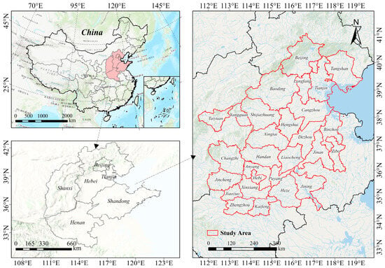
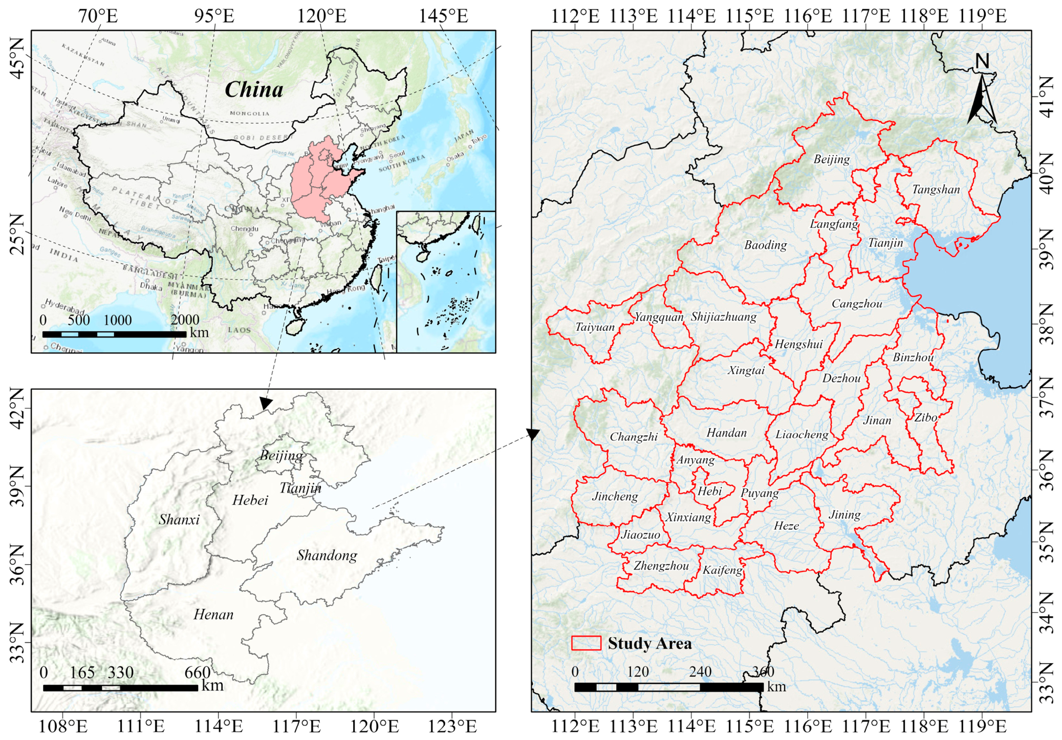
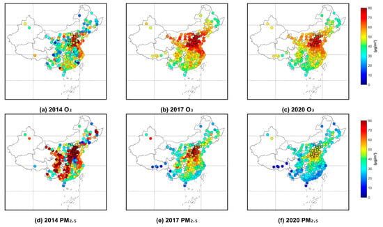
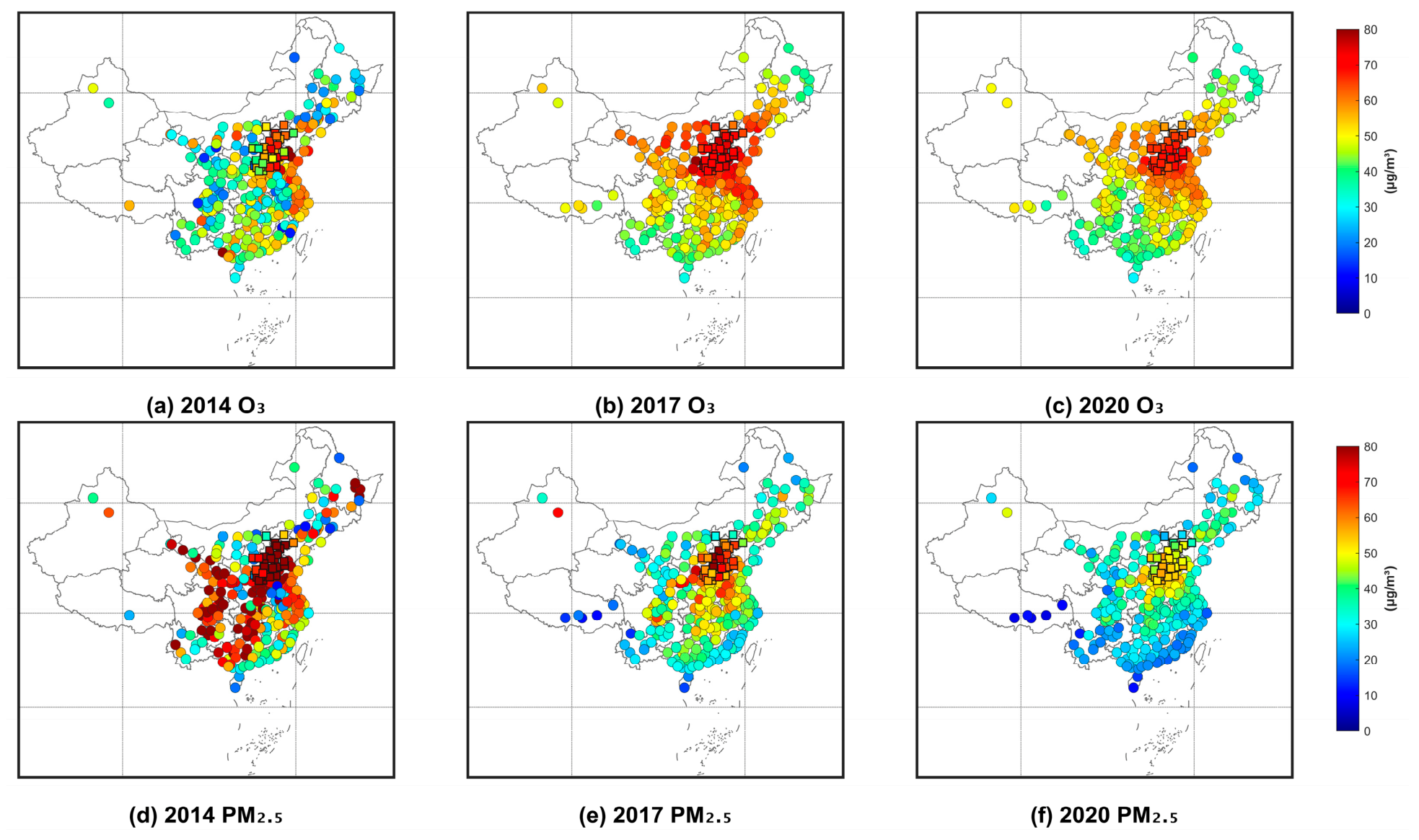
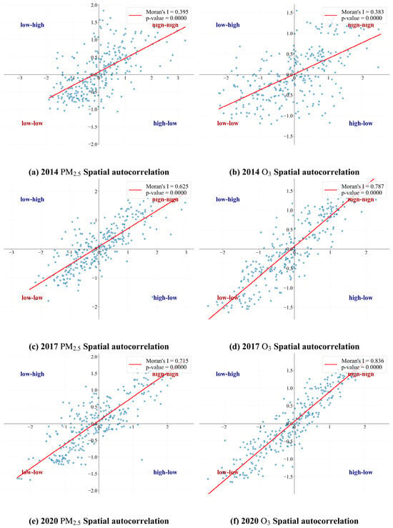
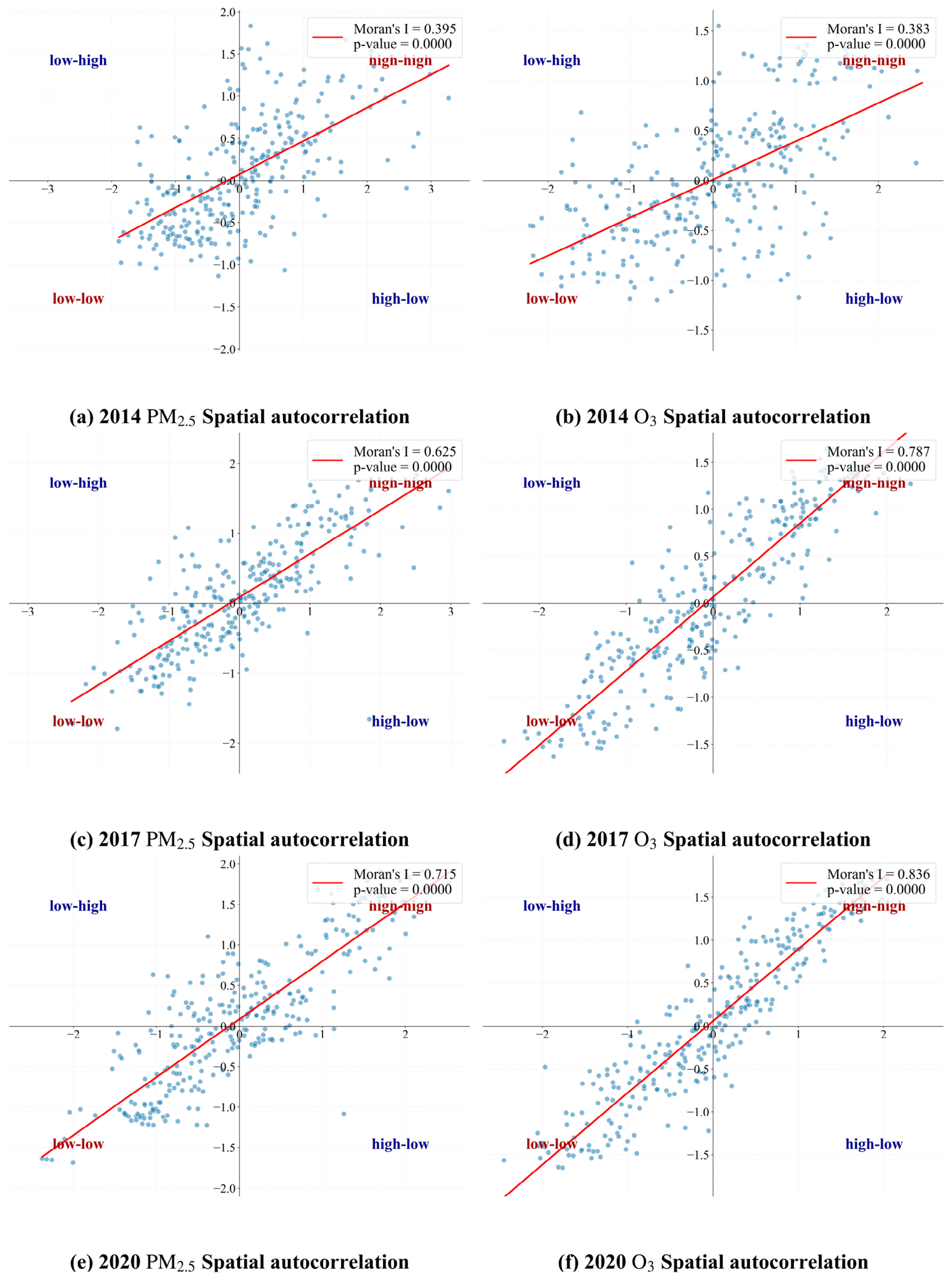
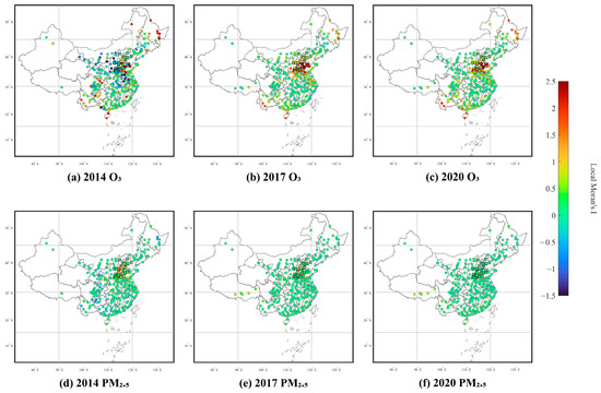
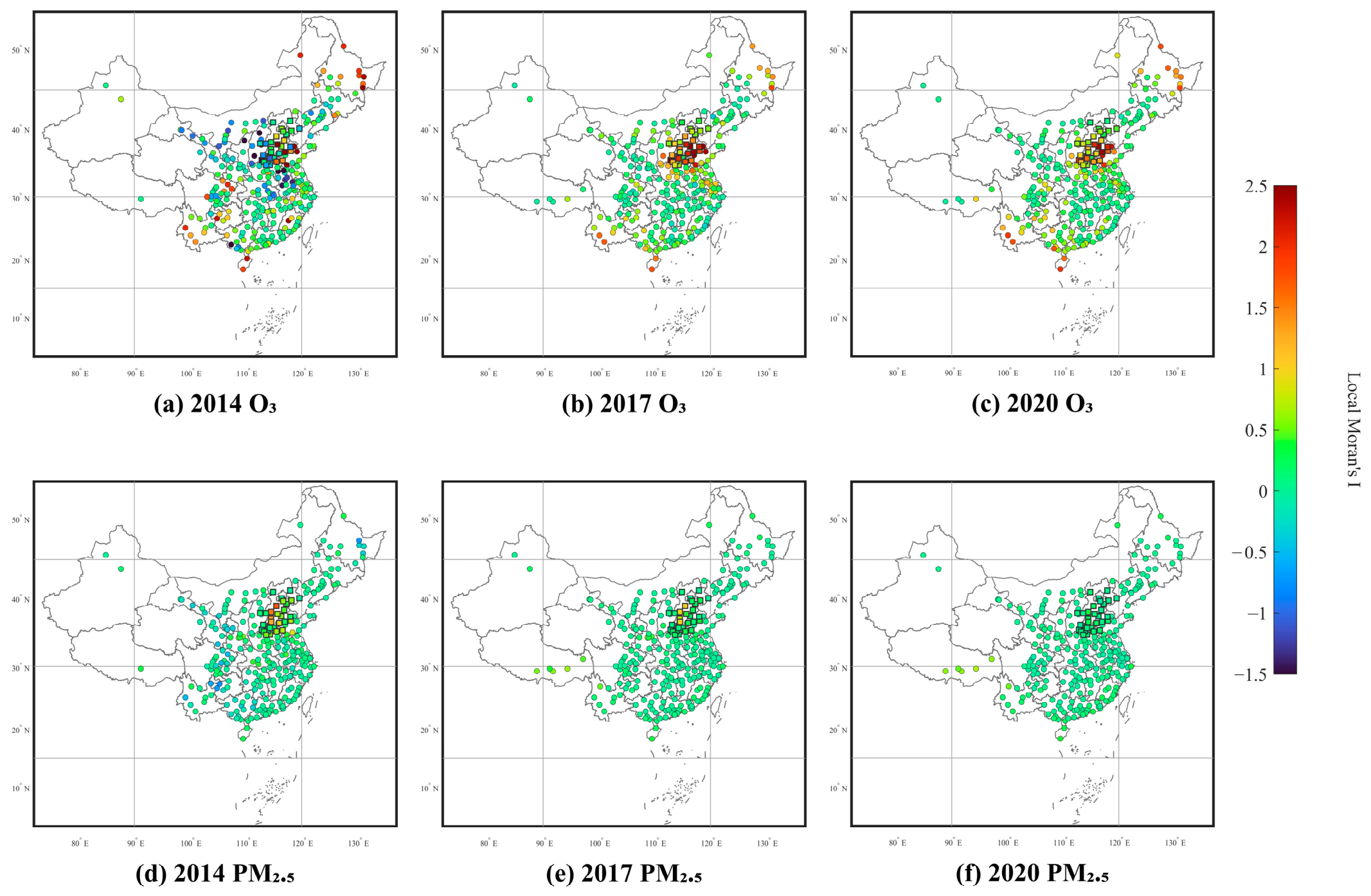
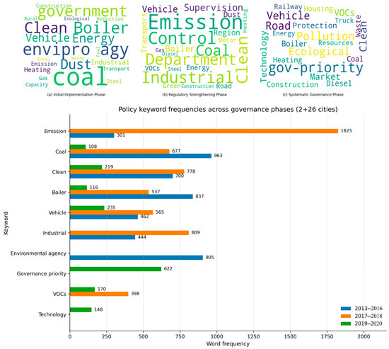
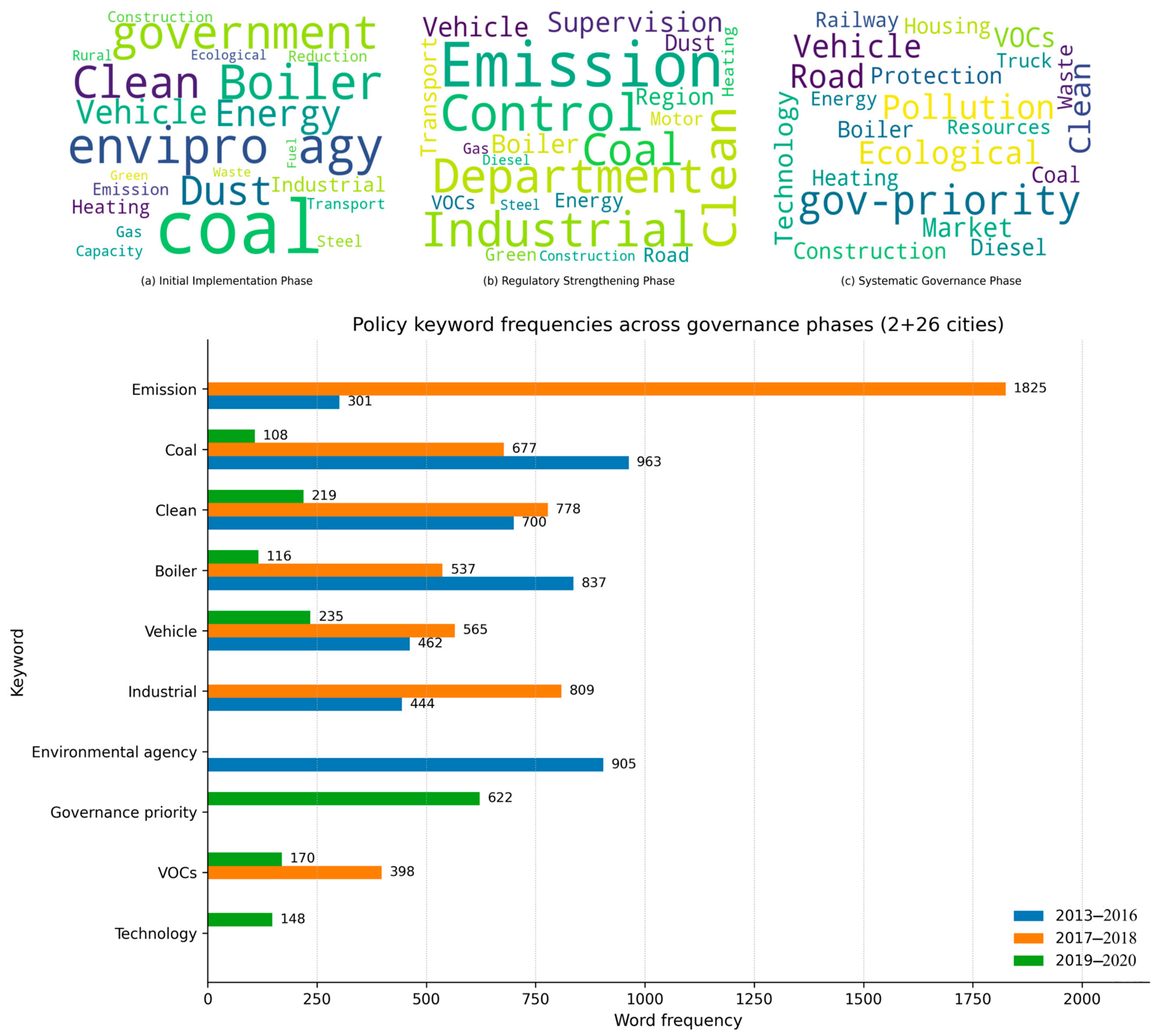

Disclaimer/Publisher’s Note: The statements, opinions and data contained in all publications are solely those of the individual author(s) and contributor(s) and not of MDPI and/or the editor(s). MDPI and/or the editor(s) disclaim responsibility for any injury to people or property resulting from any ideas, methods, instructions or products referred to in the content. |
© 2026 by the authors. Licensee MDPI, Basel, Switzerland. This article is an open access article distributed under the terms and conditions of the Creative Commons Attribution (CC BY) license.