


Abstract
Consumption-side regulation and production-side regulation are both important approaches to environmental policy. To effectively formulate targeted regulatory measures and support long-term sustainable development, environmental performance must first be accurately assessed. The Leontief optimization method has been proposed to assess environmental performance on the production side for multi-sector economies. However, no effective assessment tool is currently available on the consumption side. Furthermore, studies have not fully analyzed the differences in environmental performance assessment between the consumption and production sides. This means there is a lack of technical guidance for decision-makers in terms of selecting and applying appropriate methods. To address these problems, this article first proposes the Ghosh optimization method to fill the assessment tool gap on the consumption side. Second, the theoretical difference between the two methods is compared, including the theoretical basis, optimization objective, and inefficiency tracing. Finally, the tools are applied to analyze the case study of CO2 emissions in China. This analysis demonstrates the differences in emissions reduction potential between the consumption and production sides. The results verify this study’s propositions regarding optimization objectives and inefficiency tracing. The article concludes that, to reduce carbon emissions more efficiently and achieve sustainability goals, China must focus attention on addressing the emission reduction potential from consumption.
1. Introduction
Industrial production activities constitute the primary source of direct environmental contaminants and greenhouse gas emissions [1,2,3], hindering long-term global sustainability. Precisely for that reason, environmental regulatory frameworks predominantly target the production sector through diverse constraint policies. Industrial restructuring serves as a prevalent meso-level environmental governance instrument, which has been extensively implemented across major economies, including China [4], Japan [5], and the European Union [6], to reconcile economic growth with sustainability. At the micro enterprise level, governments have combined administrative mandates and market-oriented incentives in their environmental governance strategies. Common regulatory measures include stringent emission criteria [7,8], environmental taxation systems [9,10], and tradable environmental rights mechanisms [11,12].
Accurately evaluating environmental performance is the fundamental foundation of rational policy formulation. This makes production-side environmental efficiency a pivotal research hotspot in the field of environmental economics. Due to the method’s unique strength in simulating undesirable outputs, data envelopment analysis (DEA) has gained widespread popularity in environmental performance evaluation [13]. For instance, Vlontzos et al. [14] adopted a non-radial DEA model to quantify the agricultural environmental efficiency of EU member states between 2001 and 2008. The study’s empirical results indicated that regions with rigorous environmental regulations actually tend to exhibit lower environmental efficiency. Extant DEA-based environmental assessment research has also extended to various industrial sectors, including service industries [15], transportation [16], power generation [17], manufacturing [18], and construction [19].
Nevertheless, the aforementioned studies are confined to individual industrial sectors; they ignore intrinsic production correlations across diverse industries. The result of this approach is compromised estimation accuracy and poor traceability of emission sources. To fill this research gap, Mahlberg and Luptáčik [20] developed a Leontief input–output optimization model to evaluate multi-sector environmental performance. Importantly, this model also considers inter-sectoral production linkages. On this basis, Wang et al. [21] further proposed the generalized Leontief input–output (GLO) optimization approach, which enables the identification of environmental improvement potential by adjusting input coefficients and environmental intensity indicators. Collectively, these methodological innovations exclusively focus on production-side environmental evaluation.
Apart from production-oriented environmental governance, consumption-side management is another indispensable approach to improving ecological quality and achieving holistic sustainability [22,23]. This perspective is particularly applicable to scenarios in which environmental degradation stems from consumption patterns, rather than from production inefficiencies [24]. In terms of intermediate consumption, the effective management of power demand has become a typical solution used to address the inherent volatility and intermittency of renewable energy [25]. Additionally, guiding end consumers to adopt eco-friendly consumption behaviors has been verified to effectively curb pollutant emissions [26,27,28].
Despite the proven significance of consumption-side governance, academic research in this field remains both insufficient and underdeveloped. Only a limited number of studies have even attempted consumption-based environmental performance assessment. For example, Zurano-Cervelló et al. [29] measured the environmental performance of 14 European manufacturing industries by incorporating consumption-based emission data into a DEA framework. Similarly, Wang et al. [30] and Wang et al. [31] conducted cross-country environmental performance research from the perspective of global supply chains. Admittedly, these studies shifted the research perspective from production to consumption. However, importantly, inter-sectoral production linkages were still overlooked. As emphasized by Wang et al. [21], such research merely transforms the “black box” from being production-based to being consumption-based. Therefore, an urgent need exists to develop a targeted analytical tool that can achieve precise and traceable consumption-side environmental performance measurements to support sustainability policymaking.
This discussion reveals several key research issues regarding the effective evaluation of environmental performance across multi-sector economies. It is necessary to develop a generalized Ghosh input–output optimization (GGO) method based on the existing GLO framework for consumption-side environmental performance assessment. Theoretical exploration is also required to clarify the distinctions between the GGO and GLO approaches, as well as the new information derived from comparative analysis of production-side and consumption-side environmental results. This article targets the above issues and related underlying challenges and presents three major contributions to the existing literature.
First, this article proposes the GGO method under two substitution assumptions, providing a reliable tool for assessing environmental performance on the consumption side. The article also theoretically compares the GGO and GLO methods, clearly differentiating between the two methods with respect to the theoretical basis, optimization objective, and inefficiency tracing. In this article, the consumption-side environmental inefficiency quantified via the GGO model denotes emission abatement potential obtainable by restructuring resource allocation, covering both intermediate use and final demand configurations. By contrast, production-side environmental inefficiency estimated with the GLO model corresponds to mitigation potential unlocked through revisions to input composition, including the structures of intermediate and primary inputs. Finally, a CO2 case study for China is used to verify propositions about the GGO and GLO methods and to analyze the difference in CO2 emission reduction potential between the consumption and production sides in China, offering clear implications for national sustainable carbon management.
The remaining sections of this article are organized as follows: Section 2 proposes the basic GGO method and then compares the GGO and GLO methods. Section 3 empirically analyzes the GGO and GLO models. Section 4 presents a CO2 case study for China, and Section 5 concludes the article and provides policy insights for sustainable low-carbon transition in China.
2. Theoretical Comparison Between the Leontief and Ghosh Methods
The Leontief input–output optimization model is built on the Leontief input–output analysis framework. Specifically, the GLO model optimizes the sectoral structure of primary input by establishing constraints of row-oriented balance (regarding the final demand by each sector and the aggregated primary input of all sectors), thereby uncovering the potential for emission reduction. Under the Ghosh input–output analysis framework, the Ghosh input–output optimization model is constructed. In the GGO model, the sectoral structure of final demand is optimized to assess environmental performance by establishing constraints of column-oriented balance (regarding the primary input by each sector and the aggregated final demand of all sectors).
2.1. The Basic Generalized Ghosh and Leontief Input–Output Optimization Model
Assuming an economy consists of () sectors, each sector uses () primary inputs () to produce goods, meets () final demand (), and generates () environmental factors () (e.g., environmental pollution and greenhouse gases). The total output of each sector is defined as . The total amount of each input–output factor in an economy is represented by the corresponding capital letters. For example, the total amount of the primary input in an economy is . The basic GGO model is expressed in Equation (1).
In Equation (1), () represents different periods. The terms , , and represent the potential intermediate use matrix, potential final demand matrix, and potential environmental factor intensity matrix, respectively. The term represents the potential total output vector; represents the origin vector associated with the total primary input of each sector; represents the origin vector associated with the total final demand of each type; represents the original vector associated with the total environmental factor of each type; and represents the weight matrix for constructing , and . The term is the scale factor vector of environmental factors used to assess environmental inefficiency. The symbol represents the Hadamard product. The superscript represents the transpose of a vector or matrix. Constraint (1b) ensures the potential added value of each sector is not less than the original value. Constraint (1c) adjusts the sectoral structure of final demand without exceeding the original final demand. Constraint (1d) and objective function (in Equation (1), environmental factors are considered equivalent. If the importance of environmental factors differs, different weights are assigned to them in the objective function) maximize the improvement potential of environmental factors. When there are () available combinations of coefficient matrices ( and ) and environmental factor intensity matrix (), the resulting , , and are shown in Equation (2).
In Equation (2), , , and represent the weight matrices for , , and , respectively. The term represents the proportion of goods from sector consumed by sector ; this is the intermediate use coefficient from sector to sector . The term represents the proportion of goods from sector used to meet final demand ; this is the final demand coefficient from sector to final demand . The term represents the environmental factor intensity of sector . The weights associated with all , , and terms for sector are the same. This is because the usage structure of goods and environmental intensities from sector is considered to be an indivisible whole. This assumption ensures that potential production technologies are realistically feasible. Further, ensures a balanced relationship between total input and total output, as shown in Proposition 1 and Proof below. The superscript represents the optimal value calculated using Equation (1).
Proposition 1.
The optimal gross output () is equal to the optimal gross input () for each sector in Equation (1).
Proof.
is rearranged as . Given that , and , then . Therefore, is equal to .□
is changed to , given that . For the convenience of solving, Equation (1) must be transformed into a linear programming problem. Assuming , this yields and . This is the case because the elements of each column in the matrix have the same value. Therefore, Equation (1) is then expressed as Equation (3), the basic GGO model under the non-zero substitution elasticity assumption is shown in the Appendix A, where , and represents the transposed vectors of .
The basic GLO model is transformed into a linear programming problem, as shown in Equation (4). Additional details can be found in Wang et al. [21]. In Equation (4), and represent the available intermediate input coefficient matrix and primary input coefficient matrix, respectively. The term represents the origin vector associated with the total final demand of each sector; represents the origin vector associated with the total primary input of each type; is the scale factor vector of environmental factors to assess environmental inefficiency, and is the vector of the product of potential weight and potential total output, similar to in Equation (3).
2.2. Ghosh Method Versus Leontief Method
From a theoretical perspective, the GGO and GLO methods are both extensions of input–output (IO) technology. However, the two methods take different optimization directions based on two basic IO models, namely the Ghosh IO model and the Leontief IO model. The GGO method in this study is built on the supply-driven Ghosh IO model [32]. In the Ghosh IO model, the total output depends on the primary input. In Equation (1), the constraints (1b) and (1c) ensure that the column balance relationship of the input–output table is satisfied. This essentially indicates that the various types of primary inputs in various sectors and the total quantity of each type of final demand significantly impact the optimization results. In contrast, the GLO method is built on the demand-driven Leontief IO model [33]. In that model, the total output depends on the final demand. In Equation (4), the constraints (4b) and (4c) ensure that the row balance relation of the input–output table is satisfied. This means that various types of final demand in various sectors and the total quantity of each type of primary input significantly impact the optimization results.
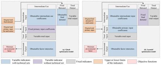
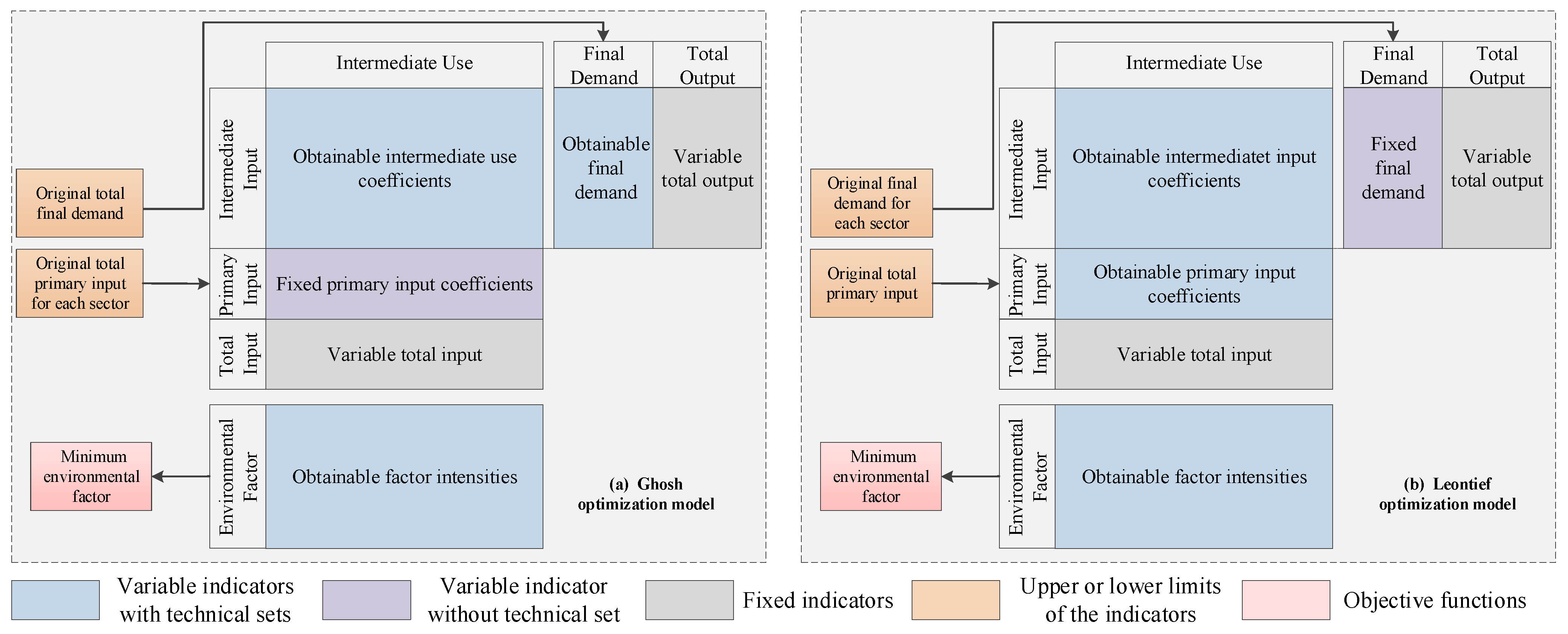
With respect to the optimization objective, comparing Equations (3) and (4) can reveal that the GGO model evaluates the consumption side performance level of multi-sector economies. Meanwhile, the GLO model focuses on the production side. Specifically, the GGO model optimizes the total output and allocation structure of goods for each sector, including intermediate use coefficients and final demand coefficients (see Figure 1). In contrast, the GLO model optimizes the total output and input structure for each sector, including intermediate input coefficients and primary input coefficients.
Figure 1.
Differences in the optimization processes between the Ghosh and Leontief methods.
This leaves the following questions: What does this mean with respect to the primary input and final demand values? In the optimal IO table, are the optimal primary input and final demand equal to the given value? The next step is to mathematically assess the difference between the optimal value and the given value associated with the primary input and final demand.
Proposition 2.
In Equation (3), the slack variables associated with constraints (3b) and (3c) are equal to zero. Therefore, the optimal solution in Equation (3) changes neither the primary input values for each sector nor the total quantity of each type of final demand.
Proof.
Combining constraint (3d) and the objective function (3a), Equation (3) is rewritten as Equation (5). According to duality theory, the duality problem of Equation (5) is shown in Equation (6). In Equation (6), and represent the dual variables of constraints (5b) and (5c), respectively. Assume is the optimal solution of Equation (6), where . Adding a similar arbitrary positive number () to each variable in yields , where . When incorporating into Equation (6), is equal to , given that . Given , is equal to . Constraint (6b) is also met, and the value of the objective function does not change. This means that is also an optimal solution for Equation (6). Therefore, the slack variable of the constraint associated with is equal to zero. Similarly, all slack variables in constraints (5b) and (5c) are shown to equal zero. Equation (5) is equivalent to Equation (3), and therefore, all slack variables in constraints (3b) and (3c) are equal to zero. Therefore, in the optimal solution of Equation (3), the optimal primary inputs for each sector and the optimal total quantity of each type of final demand are equal to the original values. The total quantity of each type of final demand does not change; however, the sector structure of each type of final demand is optimized.
□
Proposition 3.
In Equation (4), the slack variables for constraints (4b) and (4c) are equal to zero. Therefore, the optimal solution in Equation (4) changes neither the final demand values for each sector nor the total quantity of each type of primary input.
Proof.
Combining the constraint (4d) and objective function (4a), Equation (4) is rewritten as Equation (7). The duality problem of Equation (7) is shown in Equation (8), in which and are the dual variables of constraints (7b) and (7c), respectively. Assume is the optimal solution of Equation (8), where . Adding a similar arbitrary positive number () to each variable in yields , where . Incorporating into Equation (8) also meets constraint (8b). Also, the value of the objective function does not change, given that and . This means that is also an optimal solution of Equation (8). Thus, the slack variable of the constraint associated with is equal to zero. Similarly, all slack variables in constraints (7b) and (7c) are shown to equal zero. Given that Equation (7) is equivalent to Equation (4), all slack variables in constraints (4b) and (4c) are equal to zero. Therefore, in the optimal solution of Equation (4), the optimal final demand for each sector and the optimal total quantity of each type of primary input are equal to the original values. The total quantity of each type of primary input does not change; however, the sector structure of each type of primary input is optimized.
□
The different perspectives of performance assessment significantly impact estimation results and also lead to significant differences in the tracing of environmental inefficiencies. For example, when the structural decomposition analysis (SDA) method is used to identify the reduction potential of environmental factors, the reduction potential associated with primary input is zero in the GGO method. In contrast, the factor with zero emission reduction potential is the final demand in the GLO method. Adjustments have been made to the input and allocation structures of multi-sector economies in both the GGO and GLO methods. However, this does not make both methods beneficial for reducing environmental factors for each multi-sector economy. Theoretically, if the total output of each sector is not allowed to increase (see Section 3), the GGO method only ensures that the optimized allocation structure of the multi-sector economy is beneficial for reducing environmental factors. In contrast, this is the input structure in the GLO method. Using the GGO method as an example, constraint (1b) in Equation (1) is rewritten as , given that its slack variables are zero. Moreover, the total primary input of each sector does not change, and the total output of each sector can only be constant or reduced. Therefore, the Ghosh inverse matrix has a negative impact on environmental factors.
Similar phenomena also occur when using the structural path analysis (SPA) method. When the Leontief SPA model is used to trace environmental potential, in the GLO method, the reduction potential of different industrial paths is derived by adjusting environmental factor intensities and the intermediate input matrix. In the GGO method, the reduction potential may also be derived by adjusting the final demand. When the Ghosh SPA model is applied, the reduction potential of different industrial paths is derived by adjusting the environmental factor intensities and intermediate use matrix in the GGO method. The reduction potential may also be derived by adjusting primary inputs in the GLO method.
Despite its wide application in measuring forward industrial linkages, the traditional supply-driven Ghosh input–output analysis model has long been criticized for its theoretically implausible economic assumptions [34,35]. First, the core assumption of fixed allocation coefficients implies perfect substitutability of intermediate inputs across sectors, which fundamentally contradicts the fixed complementary input structure of the standard Leontief production framework. Second, the Ghosh input–output analysis model yields counterintuitive and economically paradoxical results in quantity-based simulations. Exogenous growth in value-added in a single sector can trigger output expansion across all downstream industries without any increase in primary factor inputs, and the model even allows aggregate output to rise while total value-added declines, violating the basic economic principle that output growth relies on factor input accumulation [36,37]. For these reasons, scholars generally recommend abandoning the original Ghosh quantity interpretation and reinterpreting the Ghosh inverse as a cost-push price transmission model for sustainable and carbon-related analysis [38].
The proposed Ghosh input–output optimization model is more suitable for analyzing demand-side environmental potential and can avoid the aforementioned limitations of the Ghosh input–output analysis model. First, the proposed input–output optimization model adopts a modeling logic different from that of traditional input–output analysis models. The demand-driven Leontief input–output analysis model determines total output by final demand and is applied to demand-side analysis. In the Leontief input–output optimization model, however, sectoral demand and aggregate value-added are fixed (Proposition 3), and only the sectoral structure of value-added is adjusted. Therefore, the Leontief input–output optimization model essentially optimizes the supply structure, which makes it suitable for exploring supply-side environmental potential. In contrast, the supply-driven Ghosh input–output analysis model determines total output by supply conditions and is used for supply-side analysis. Differently, the Ghosh input–output optimization model fixes sectoral value-added and aggregate demand (Proposition 2) and only adjusts the sectoral structure of demand. Accordingly, the Ghosh input–output optimization model takes demand structure as its optimization objective, which renders it suitable for tapping demand-side environmental potential.
Second, the allocation coefficients in the proposed Ghosh input–output optimization model are not fixed but optimized within technically feasible boundaries. The Ghosh input–output optimization model takes technically feasible allocation structures as the basis for adjustment and regards each feasible allocation structure as an integral whole, ensuring the practical feasibility of optimized allocation structures in reality. In addition, large-scale adjustments of allocation structures are inconsistent with short-term economic rules. For this reason, the empirical model (see Section 3) introduces multiple constraints on the basis of the standard Ghosh input–output optimization model to control the adjustment scale of allocation structures. Specifically, 70% of industrial output is allocated following the original baseline structure, and the adjustment range of sectoral demand is limited to within 10%. These settings avoid abnormal fluctuations in allocation structures and improve the accuracy of environmental potential assessment.
3. Empirical Model
Section 2 compared the differences between the GGO and GLO methods when theoretically used to evaluate environmental performance. The basic models, however, lack range constraints with respect to emission intensity, total output, final demand, and primary input. As such, the models do not simulate the situation in reality. To more specifically show the differences between the two methods, this section builds empirical models that align with real-world situations. Empirical models can yield more accurate and feasible environmental performance assessment results. Therefore, they can be directly applied to the analysis of actual environmental issues, such as the carbon dioxide emission example in China presented in Section 4.
3.1. The Ghosh Optimization Model and Potential Decomposition Model
The empirical model associated with the GGO method is in Equation (9). Compared with Equation (1), six new constraints are added to Equation (9) to make the assessment results more consistent with real-world situations.
In Equation (9), Proposition 2 and Proposition 3 remain valid in the empirical models. The proof is similar to the relevant content in Section 2 and is not repeated here, represents the potential final demand coefficient vector associated with the type of final demand. The terms and represent the upper and lower bounds, respectively, with respect to changes in final demand. The term is the potential environmental factor intensity vector associated with the type of environmental factor. The terms and represent the upper and lower bounds, respectively, with respect to changes in environmental factor intensity.
The first three constraints are consistent with Equation (1). To avoid structural adjustments that make the sector unable to meet basic social needs, constraints (9e) and (9f) limit the range of changes in the types of final demand for each sector. To ensure that adjustments in environmental factor intensity are feasible in terms of technology and cost, constraints (9g) and (9h) limit the range of changes in the types of environmental factor intensities for each sector. Constraints (9i) and (9j) limit the range of changes in total output for each sector. Together, constraints (9g)–(9j) set upper and lower bounds for the total changes in environmental factors for each sector. When Equation (9) is transformed into a linear programming problem, Equation (9) takes the form of Equation (10).
The terms , , , , and are the optimal values returned when solving Equation (10). This yields the potential input–output table. The potential intermediate input coefficient matrix () and potential primary input coefficient matrix () are calculated using the GGO method. The Ghosh inverse matrix () and Leontief inverse matrix () are also generated. Taking the environmental factor as an example, the SDA method is used to trace the reduction potentials of environmental factors, as shown in Equations (11) and (12).
In Equation (11), the reduction potential of the environmental factor is decomposed into three parts: the structure of primary input (), the structure of production output (), and the environmental factor intensity () [39]. The term assesses the contribution of changes in the sectoral structure of primary inputs to the variation in environmental factors. It captures the environmental impact of shifts in the relative shares of primary inputs across sectors. The term quantifies the contribution of variations in the Ghosh inverse matrix to total environmental factors, isolating how shifts in allocation structure affect aggregate environmental performance. The term assesses the contribution of changes in sectoral environmental factor intensity to the variation in total environmental factors. It captures efficiency improvements or technological change in production processes.
In Equation (12), the reduction potential is decomposed into the environmental factor intensity (), the structure of production input (), and the structure of final demand () [40]. The term assesses the contribution of changes in the Leontief inverse matrix to the variation in environmental factors, capturing the environmental impact of adjustments in input structure. The term quantifies the contribution of changes in the structure of final demand to the variation in environmental factors. It captures the environmental impact of shifts in the relative shares of final demands across sectors. The terms and represent the weight coefficients in the Ghosh and Leontief decomposition models, respectively.
3.2. The Leontief Optimization Model and Potential Decomposition Model
To increase the feasibility of the optimization results, new constraints are added to the basic Leontief model to limit changes in the ranges of potential variables, as shown in Equation (13). In Equation (13), represents the potential primary input coefficient vector associated with the type of primary input. The terms and represent the upper and lower bounds, respectively, with respect to changes in primary input. Constraints (13b)–(13d) are consistent with Equation (4). To avoid industry structure changes that do not conform to development laws and planning schemes, constraints (13e) and (13f) limit the changes in the types of primary input for each sector. Constraints (13g)–(13j) are consistent with constraints (9g)–(9j) in Equation (9). Equation (13) is then transformed into a linear programming problem, shown in Equation (14).
The terms , , , and are the optimal values found by solving Equation (14). This yields another potential IO table. The potential intermediate use coefficient matrix () and potential final demand coefficient matrix () are calculated using the GLO method. The Ghosh inverse matrix () and Leontief inverse matrix () are then generated.
The SDA method is used to trace the reduction potential of the environmental factor under the GLO framework, as shown in Equations (15) and (16). The six decomposed factors share the same definitions as Equations (11) and (12), and are not restated herein. The terms and represent the weight coefficients in Equations (15) and (16), respectively.
4. A Case Study Examining CO2 Emissions in China
4.1. Research Objective and Background
Climate change has caused serious harm to global economic development [41], residents’ health [42], and the ecological environment [43]. Thus, climate change has become the most severe challenge facing mankind in the 21st century. Carbon dioxide (CO2) is the main culprit in climate change. Therefore, determining how to cost-effectively control and reduce CO2 emissions has become an important issue of global concern [44]. China’s coal-dominated energy structure has produced an enormous amount of CO2 emissions alongside the country’s economic growth. Data show that China contributes about one-third of the global emissions [45,46]. Therefore, China will play a key role in the global response to climate change [47].
It is crucial that the plans being formulated to abate CO2 emissions can also accurately identify the scale and composition of CO2 emission reduction potential [48,49]. Faced with this urgent situation, China needs to take active emission reduction measures on both the production and consumption sides. Only by addressing both production and consumption can emission reduction potential be fully unlocked [50,51]. Based on the above background, this study chooses China’s carbon emissions to conduct an empirical analysis.
4.2. Data Source and Processing
The IO tables for 2012 and 2017 at the provincial level in China are from the China Regional Input–Output Table. This study merges the provincial input–output tables for three sectors: the agricultural sector, the industrial and construction sector, and the service sector. To demonstrate the robustness of the GGO model, this article also calculated the GGO model results for the 24-sector case (see Table A1 and Table A2 in Appendix B for details). The original data and code are provided in the Supplementary Materials. Despite the fact that finer sectoral classification amplifies constraints within the GGO model and curbs its emission reduction potential, the fundamental conclusions hold steady. Due to the lack of available data, Tibet, Hong Kong, Macao, and Taiwan are excluded. Based on Wang et al. [21], the provincial input–output tables are converted to constant prices for 2012. The data for CO2 emissions created by 17 types of fossil fuel combustion are calculated using Shan et al. [52] and Shan et al. [53]. The data for CO2 emissions in eleven industrial processes, including cement and iron, are calculated using Yu and Tan [54].
For study feasibility and to support real-world practicality, this study assumes that each type of final demand or primary input for each sector varies by no more than 10%. The upper limit of the change in environmental factor intensity is the initial value; the lower limit is 95% of the initial value. The change in total output has an upper limit of the initial value and a lower limit of zero.
4.3. Scale Difference in CO2 Emission Reduction Potential
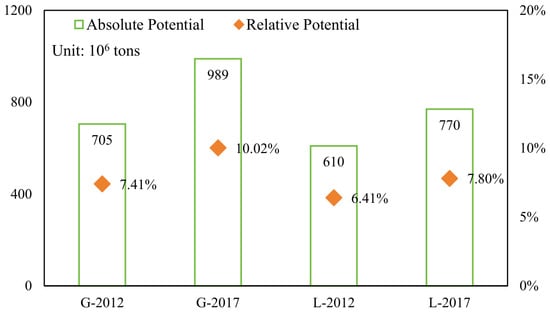
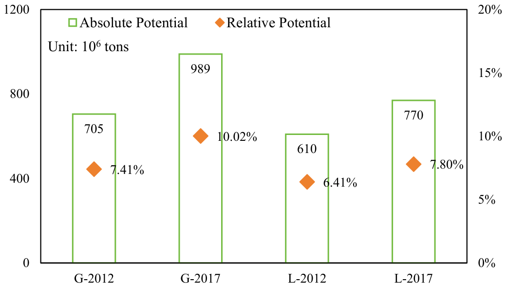
Figure 2 shows the scale difference in CO2 emission reduction potential (CERP) at the national level when comparing the GGO and GLO models. In Figure 2, G-2012 presents the calculation results for 2012 data based on the GGO model; L-2017 presents the calculation results for 2017 data based on the GLO model. Other symbols follow this pattern. In Figure 2, the national-level CERP is significantly higher when calculated using the GGO model compared to using the GLO model. Specifically, the absolute CERP values calculated using the GGO model are 705 and 989 million tons in 2012 and 2017, respectively. Notably, these levels are 95 and 219 billion tons higher, respectively, than the results calculated using the GLO model. In terms of relative CEPR, the differences in emissions reduction are 1.00% and 2.22% in 2012 and 2017, respectively. This finding indicates that the CERP on the consumption side exceeds that on the production side. Therefore, while the production side is the direct source of carbon emissions, releasing the CERP of the consumption side is also important. To realize the country’s dual-carbon goal, China needs to optimize the intermediate use structure of production activities and guide green consumption with respect to final demand.
Figure 2.
CERP comparison at the national level.
The results of the GGO and GLO models are consistent with respect to time change trends. Results from both models show a significantly increasing trend from 2012 to 2017, reflecting China’s increased CERP on both the consumption and production sides. The increase in absolute CERP relates both to the scale of China’s carbon emissions and the reduction in emissions efficiency. During the sampled years, carbon emission efficiency drops by 2.61% on the consumption side and by 1.40% on the production side. Further, the gap between consumption-side and production-side CERP widens. This gap more than doubled in 2017, compared with 2012. This reinforces the importance of reducing emissions on the consumption side.
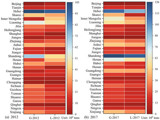
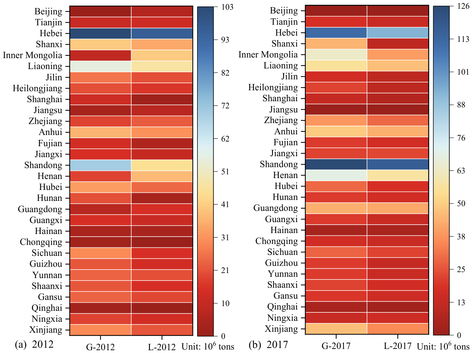
At the provincial level, there is also a significant difference in CERP between the consumption side and production side (see Figure 3). In 2012, data for Hebei Province show the highest CERP, reaching 103 billion tons on the consumption side and 96 billion tons on the production side. In contrast, Shandong Province ranked first with respect to the scale of CERP in 2017, reaching 126 billion tons on the consumption side and 117 billion tons on the production side. In contrast to the national-level data, the scale of CERP on the consumption side is not always greater than on the production side at the provincial level. Specifically, the CERP on the production side is higher than the consumption side for seven provinces. Of these, Inner Mongolia’s production-side CERP is more than four times larger than the consumption-side CERP.
Figure 3.
CERP comparison at the provincial level.
Data for 2017 show that the scale of CERP on the production side is greater than on the consumption side in only three provinces: Jiangxi, Hainan, and Ningxia. The difference is greatest in Hainan Province, where the production-side CERP is only 25 percent than the consumption-side CERP. These results highlight the growing importance of consumption-side CO2 emissions mitigation and also highlight the importance of provincial heterogeneity in policy-making. Critically, more attention must be paid to unlocking the CERP of key provinces (such as Shandong Province) and to identifying the distribution of consumption-side and production-side CERP in different provinces.
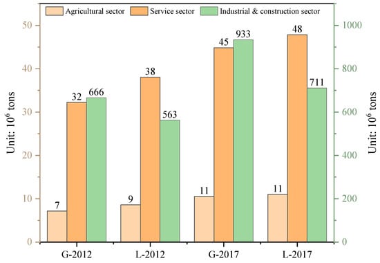
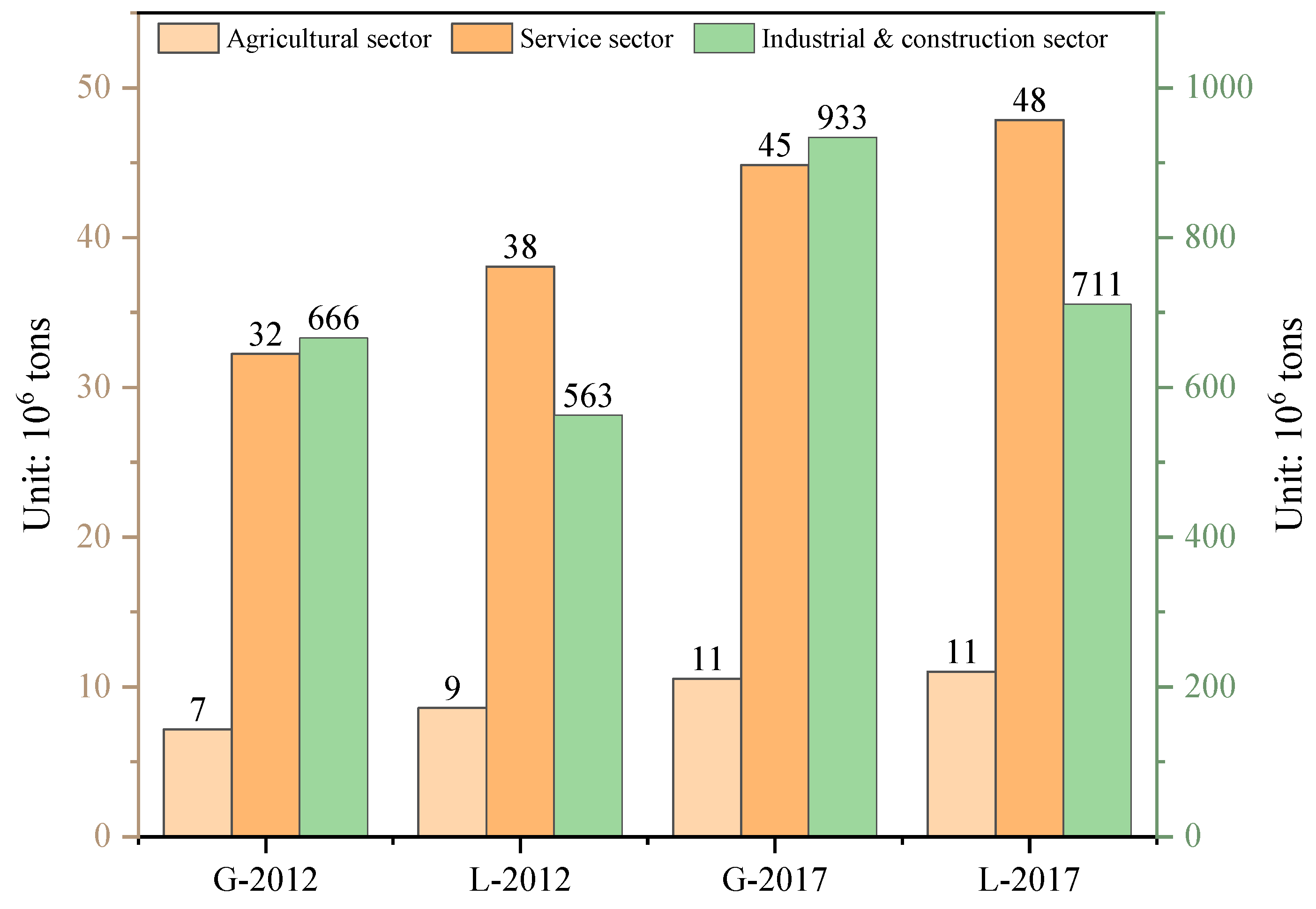
At the sector level, the industrial and construction sector dominates both production-side and consumption-side CERP; this sector’s CERP accounts for 92% to 94% of total CERP (see Figure 4). Consistent with previous research, this study finds that industrial and construction sectors are the key sectors in which to unlock CERP. Two types of scale differences exist with respect to consumption-side and production-side CERP. For the agricultural sector and service sector, the consumption-side CERP is slightly lower than that of the production side. In the industrial and construction sector, the CERP is significantly higher on the consumption side than on the production side. Specifically, the gap between the consumption-side and production-side CERP does not exceed six million tons in the agricultural sector and service sector. However, for the industrial and construction sector, the consumption-side CERP values are 103 and 222 million tons higher than the production-side CERP values in 2012 and 2017, respectively. This finding indicates that the industrial and construction sector drives the scale differences with respect to consumption-side and production-side CERP values. Further, the gaps between the consumption-side and production-side CERP in the agricultural sector and service sector are narrowing, while the gap in the industrial and construction sector widens.
Figure 4.
CERP comparison at the sectoral level.
4.4. Source Differences in CO2 Emission Reduction Potential
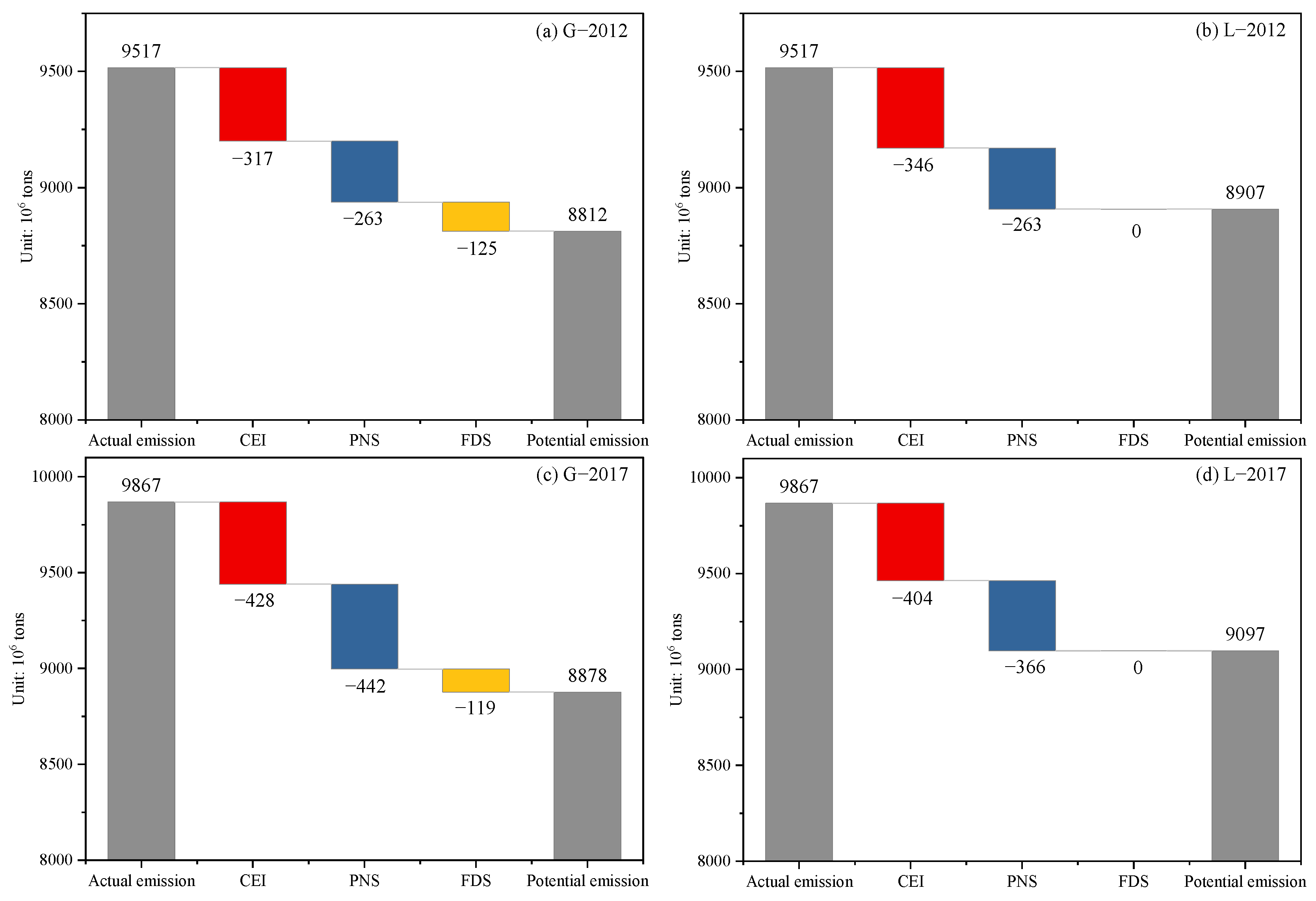
This section analyzes the differences in CERP sources between the consumption and production sides. Figure 5 shows the decomposition results based on Leontief SDA. With the GLO method, the reduction potential created by adjusting the final demand structure is zero. In contrast, with the GGO method, the average CERP associated with final demand is 122 billion tons. This verifies Proposition 3 in Section 2. Further, the CERP associated with the other two factors (adjusting emission intensity and input structure) continues to show a significant difference between the two optimization methods. In 2012, the CERP associated with adjusting emission intensity is higher when the GLO method is used; the CERP associated with the production input structure is roughly equal when comparing the two methods. However, the CERP values associated with the two factors are higher when applying the GGO method in 2017. When applying GGO and GLO methods, the CERP values associated with the emission intensity and structure of production input both increase from 2012 to 2017. Only the CERP associated with the final demand decreases, reducing from 125 to 119 million tons. This means that, when the CERP is traced from the production side, both the GGO and GLO models find that the CERP is concentrated in the production process, rather than the final consumption stage.
Figure 5.
National-level results using Leontief SDA.
Table 1 shows the provincial decomposition results using Leontief SDA. At the provincial level, the PNS in the GGO method does not dominate all provinces’ CERP values. For example, the CERP from adjusting emission intensity accounts for more than half of the total CERP in Shanxi Province when using both the GGO and GLO methods. When comparing the two methods, the CERP values resulting from adjusting emission intensity using the GLO method are higher than when using the GGO method for more than two-thirds of China’s provinces. The opposite is true for the CERP from adjusting the production input structure. The CERP values resulting from adjusting the production input structure using the GGO method are higher than those obtained when using the GLO method for 2012 and 2017 for 57% and 73% of provinces, respectively. This outcome indicates that adjusting the final demand structure may help optimize the production input structure. However, to minimize CO2 emissions, the CERP of FDS and PNS may also be negative in a few provinces (e.g., Beijing, Fujian, and Chongqing) when using the GGO method. This finding aligns with the theoretical expectations regarding tracing inefficiencies in Section 2.
Table 1.
Provincial results based on Leontief SDA (Unit: 106 tons).
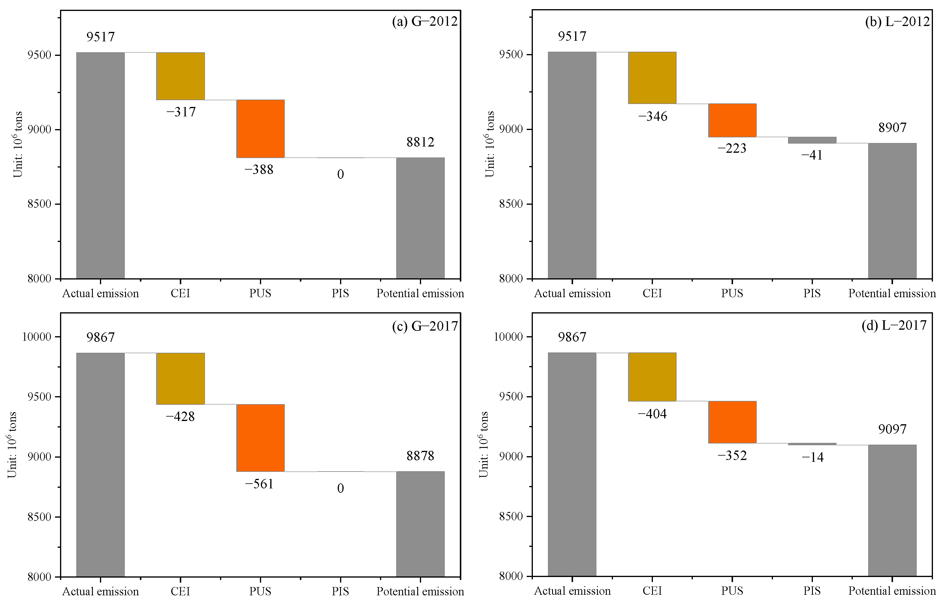
Figure 6 shows the decomposition results using the Ghosh SDA at the national level. When using the GGO method, the reduction potential from adjusting the primary input structure is zero. When using the GLO method, the average CERP of PIS is 27.5 billion tons. This result verifies Proposition 2 in Section 2. For CEI and PUS, only the potential of CEI in 2012 is lower using the GGO method, compared to the GLO method. Similar to the results of the Leontief SDA, the CERP of the product production process is significantly higher than the CERP of the industrial structure. This means the CERP is concentrated in the production process.
Figure 6.
National-level results using Ghosh SDA.
For China, optimizing the industrial chain and reducing intermediate inputs are more important actions for reducing carbon emissions than adjusting the industrial structure and final demand structure. The trend of change in the potentials of CEI and PUS is similar when comparing the two methods. The potentials of both CEI and PUS increase during the sample period. However, the PIS potential decreased from 41 billion tons in 2012 to 14 billion tons in 2017. This further highlights the importance of reducing emissions intensity and optimizing the production output structure.
Table 2 shows the Ghosh SDA decomposition results at the provincial level. The PUS in the GGO method does not dominate all provinces’ CERP values. For example, the CERP of CEI accounts for more than half the total CERP in Heilongjiang Province. This is another reminder of the heterogeneity associated with carbon reduction, which should encourage provinces to implement targeted measures and policies to reduce emissions. As for CEI, in most provinces, the CERP values resulting from adjusting the emission intensity with the GLO method are higher than those obtained with the GGO method. The result is the opposite with respect to the potential of PUS. Moreover, the potential of PUS and PIS in some provinces (e.g., Hunan and Sichuan) is negative when applying the GLO method. This indicates that adjusting the industrial structure has limited emission reduction potential and has no significant promoting effect on the production output structure.
Table 2.
Provincial results based on Ghosh SDA (Unit: 106 tons).
5. Conclusions
Breaking the black box of environmental performance assessment in multi-sector economies can provide useful information for those formulating environmental regulation policies. Both production and consumption perspectives are vital for evaluating environmental performance. The generalized Leontief input–output optimization (GLO) method has been proposed for production-side assessment, but tools for assessing the consumption side have been lacking. Further, differences in environmental performance assessment between the production side and consumption side have not been thoroughly or adequately compared. This hinders the development and perfection of assessment methods and makes it difficult for decision-makers to choose appropriate assessment methods. This study proposes the general Ghosh input–output optimization (GGO) method as an effective tool for assessing environmental performance on the consumption side. Then, the theoretical differences in environmental performance assessment between the consumption side and production side are compared, including theoretical basis, optimization objective, and inefficiency tracing. Finally, the tools are applied to analyze the potential for reducing CO2 emissions in China on both the consumption and production sides. The main findings and conclusions are as follows:
The GGO method, which is based on the Ghosh IO model, effectively assesses consumption-side environmental performance. The optimal values of primary inputs for each sector and the optimal total quantity of each type of final demand are equal to their given values in the GGO method. This means the improvement potential of the primary input is consistently zero when the environmental inefficiency is traced. In contrast, the GLO method, which is based on the Leontief IO model, assesses environmental performance on the production side. As such, environmental performance on the production side is significantly affected by the different types of final demands in each sector and the total quantity of each type of primary input. Similarly, their optimal values are equal to the given values in the GLO method; the improvement potential of the final demand is consistently zero. When policymakers focus on consumption-oriented environmental governance, the GGO method stands out as the more appropriate analytical tool due to its inherent focus on the consumption side. For initiatives targeting production-side pollution abatement and input efficiency improvement, the GLO method is better suited to capture relevant characteristics and provide reliable evaluation results. In practical environmental management, both production and consumption links play irreplaceable roles in pollution control and emission reduction. Accordingly, integrating GLO and GGO methods is necessary to conduct a comprehensive assessment and formulate holistic governance strategies.
In China, during the study period, the total reduction potential of CO2 emissions is significantly higher on the consumption side than on the production side. This points to the need for China to focus on potential consumption-side emission reductions. Refining industrial intermediate input structures and promoting green consumption from the final demand perspective constitute indispensable policy priorities for China. This requires not only targeted technological upgrades but also differentiated consumption incentive policies. For instance, targeted R&D investment in core technologies accelerates the low-carbon shift in energy-intensive industries, while tiered subsidies for new-energy vehicles and high-efficiency home appliances steer low-carbon consumption restructuring. From 2012 to 2017, the scales of both consumption-side and production-side potential increased significantly, while the emission efficiency decreased. China needs to invest greater effort and commitment to advance the stated dual-carbon goal of reaching the country’s carbon peak by 2030 and carbon neutrality by 2060.
Most of China’s emission reduction potential is concentrated in the production process, rather than in the final demand structure or industrial structure. Therefore, the production correlation between sectors must be urgently adjusted by innovating production technology and optimizing the industrial chain. Specifically, authorities can roll out special fiscal subsidies and tax reductions to support enterprises’ clean technology renovation and cross-industry collaborative low-carbon transformation, while introducing industrial guidance catalogs to phase out backward high-carbon intermediate input links and build low-carbon upstream–downstream industrial matching systems. Finally, China’s emission reduction potential is significantly heterogeneous across provinces and sectors. This highlights the need for relevant authorities to tailor policies to each region and sector. For instance, key high-potential provinces, including Shandong and Hebei, shall focus on consumption-side carbon governance. Inner Mongolia, Ningxia, Hainan, and Jiangxi ought to prioritize production-oriented emission control matching their higher production-side CERP. Shanxi and Heilongjiang need to center policy on lowering carbon emission intensity.
Although this study compares the GLO and GGO methods and explores China’s CO2 emission reduction potential from production and consumption perspectives, there are certain drawbacks. It merely adopts carbon emissions as the sole undesirable output while ignoring other common pollutants. Additionally, the empirical analysis is restricted to 2012–2017 due to data limitations. Correspondingly, future research can be optimized in the following ways: enrich the evaluation indicators to cover diverse pollutants for multidimensional environmental performance assessment, and extend the research period to analyze long-term efficiency evolution under relevant low-carbon policies.
Supplementary Materials
The following supporting information can be downloaded at: https://www.mdpi.com/article/10.3390/su18136486/s1, File S1: Ghosh model for 3 sectors; File S2: Ghosh model for 24 sectors; File S3: Leontief model for 3 sectors; File S4: 2012-3S-G MAT input-output dataset; File S5: 2017-3S-G MAT input-output dataset; File S6: 2012-24S MAT input-output dataset; File S7: 2017-24S MAT input-output dataset; File S8: 2012-3S-L MAT input-output dataset; File S9: 2017-3S-L MAT input-output dataset.
Author Contributions
Conceptualization, Y.W. and X.M.; Methodology, Y.W.; Software, Y.W.; Formal analysis, X.M.; Writing—original draft, Y.W. and X.M.; Writing—review & editing, X.M. All authors have read and agreed to the published version of the manuscript.
Funding
This article is supported by the National Natural Science Foundation of China (Grant No. 72174136), the Ministry of Education of China, Youth Project of Humanities and Social Sciences (Grant No. 25YJC790110), the Social Science Foundation of Jiangsu Province (Grant No. 24GLC019), and the Humanities & Social Sciences Research Project of Soochow University (Grant No. 25XM1016).
Institutional Review Board Statement
Not applicable.
Informed Consent Statement
Not applicable.
Data Availability Statement
The data and code used in this article are provided in the Supplementary Materials.
Conflicts of Interest
The authors declare no conflicts of interest.
Appendix A. Extension to Non-Zero Substitution Elasticity Assumption
Under the non-zero substitution elasticity (NIS) assumption, the allocation structure of goods for each sector is not considered to be an indivisible whole. The generalized GGO model is shown in Equation (A1).
The first three constraints in Equation (A1) correspond one-to-one with Equation (1). The term is the scale factor vector used to assess environmental performance. The terms , , and represent the weight matrices for constructing , , and , respectively. The main differences between Equation (A1) and Equation (1) are the construction methods of the potential coefficient matrices and the potential environmental factor intensity matrix. The , , and are shown in Equations (A2)–(A4).
Next, , , , and are the optimal values found by solving Equation (A1). The sum of the potential allocation coefficients is set as unity: . This ensures a balanced relationship in the potential input–output table in the GGO model under the NIS assumption.
Proposition A1.
The optimal gross output (
) is equal to the optimal gross input () for each sector in Equation (A1).
Proof.
is rearranged as . Because , is equal to . □
By letting , and , Equation (A1) is transformed into a linear programming problem as Equation (A5). In Equation (A5), , , , and . Because , , and , we obtain . Moreover, to satisfy the balance rule of the IO table, is set as unity and is equal to . Therefore, Equation (A1) is written as Equation (A5):
Appendix B. Sensitivity Analysis Associated with Sector Aggregation Schemes
Table A1.
Sector classification.
Table A2.
Provincial results of 24-sector economy (Unit: 106 tons).
References
- Liang, S.; Wang, Y.; Zhang, C.; Xu, M.; Yang, Z.; Liu, W.; Liu, H.; Chiu, A.S. Final production-based emissions of regions in China. Econ. Syst. Res. 2018, 30, 18–36. [Google Scholar] [CrossRef] [Scilit]
- Sun, Y.-F.; Zhang, Y.-J.; Su, B. How does global transport sector improve the emissions reduction performance? A demand-side analysis. Appl. Energy 2022, 311, 118648. [Google Scholar] [CrossRef] [Scilit]
- Tsukioka, A. Supply chain hotspot analysis of the Nexus between energy costs and CO2 emissions: Evidence from Japan. Energy Econ. 2026, 154, 109152. [Google Scholar] [CrossRef] [Scilit]
- Cai, J.; Huang, J.; Yang, J.; Liu, M.; Fang, W.; Ma, Z.; Bi, J. A better balance: Energy transition and industrial restructuring for a sustainable economy-climate-environment pathway. J. Environ. Manag. 2025, 381, 125265. [Google Scholar] [CrossRef] [Scilit] [PubMed]
- Tsukioka, A.; Kagawa, S. Identifying critical supply chain sources of imported inflation: Evidence from Japan. Econ. Syst. Res. 2025, 37, 335–352. [Google Scholar] [CrossRef] [Scilit]
- Teixeira, J.E.; Tavares-Lehmann, A.T.C. Industry 4.0 in the European Union: Policies and national strategies. Technol. Forecast. Soc. Change 2022, 180, 121664. [Google Scholar] [CrossRef] [Scilit]
- Hampf, B.; Rødseth, K.L. Carbon dioxide emission standards for US power plants: An efficiency analysis perspective. Energy Econ. 2015, 50, 140–153. [Google Scholar] [CrossRef] [Scilit]
- Tang, L.; Qu, J.; Mi, Z.; Bo, X.; Chang, X.; Anadon, L.D.; Wang, S.; Xue, X.; Li, S.; Wang, X.; et al. Substantial emission reductions from Chinese power plants after the introduction of ultra-low emissions standards. Nat. Energy 2019, 4, 929–938. [Google Scholar] [CrossRef] [Scilit]
- Neves, S.A.; Marques, A.C.; Silva, I.P. Promoting the circular economy in the EU: How can the recycling of e-waste be increased? Struct. Change Econ. Dyn. 2024, 70, 192–201. [Google Scholar] [CrossRef] [Scilit]
- Wu, F.; Dogan, B.; Tiwari, S.; Ghosh, S.; Bashir, M.F.; Balsalobre-Lorente, D. From policy to practice: How eco-innovation, green finance, and environmental taxes drive carbon neutrality and sustainable development. Sustain. Dev. 2026, 34, 2146–2165. [Google Scholar] [CrossRef] [Scilit]
- Dai, S.; Qian, Y.; He, W.; Wang, C.; Shi, T. The spatial spillover effect of China’s carbon emissions trading policy on industrial carbon intensity: Evidence from a spatial difference-in-difference method. Struct. Change Econ. Dyn. 2022, 63, 139–149. [Google Scholar] [CrossRef] [Scilit]
- Zeng, A.; Cheng, Y.; Liu, Y.; Zhu, T.; Liu, H. The linkage of emissions trading system and green electricity certificate brings economic benefits in China. J. Clean. Prod. 2026, 543, 147613. [Google Scholar] [CrossRef] [Scilit]
- Song, M.; An, Q.; Zhang, W.; Wang, Z.; Wu, J. Environmental efficiency evaluation based on data envelopment analysis: A review. Renew. Sustain. Energy Rev. 2012, 16, 4465–4469. [Google Scholar] [CrossRef] [Scilit]
- Vlontzos, G.; Niavis, S.; Manos, B. A DEA approach for estimating the agricultural energy and environmental efficiency of EU countries. Renew. Sustain. Energy Rev. 2014, 40, 91–96. [Google Scholar] [CrossRef] [Scilit]
- Martínez, C.I.P. An analysis of eco-efficiency in energy use and CO2 emissions in the Swedish service industries. Socio-Econ. Plan. Sci. 2013, 47, 120–130. [Google Scholar] [CrossRef] [Scilit]
- Ben Abdallah, K.; Belloumi, M.; De Wolf, D. International comparisons of energy and environmental efficiency in the road transport sector. Energy 2015, 93, 2087–2101. [Google Scholar] [CrossRef] [Scilit]
- Halkos, G.E.; Polemis, M.L. The impact of economic growth on environmental efficiency of the electricity sector: A hybrid window DEA methodology for the USA. J. Environ. Manag. 2018, 211, 334–346. [Google Scholar] [CrossRef] [Scilit] [PubMed]
- Halkos, G.; de Alba, J.M.; Bampatsou, C. Determinants of environmental efficiency and sources of productivity change in the manufacturing sector: A comparative analysis between Europe and Asia. Energy 2024, 291, 130355. [Google Scholar] [CrossRef] [Scilit]
- Zhang, J.; Ouyang, Y.; Ballesteros-Pérez, P.; Li, H.; Philbin, S.P.; Li, Z.; Skitmore, M. Understanding the impact of environmental regulations on green technology innovation efficiency in the construction industry. Sustain. Cities Soc. 2021, 65, 102647. [Google Scholar] [CrossRef] [Scilit]
- Mahlberg, B.; Luptáčik, M. Eco-efficiency and eco-productivity change over time in a multisectoral economic system. Eur. J. Oper. Res. 2014, 234, 885–897. [Google Scholar] [CrossRef] [Scilit]
- Wang, Y.; Jeong, S.; Hang, Y.; Wang, Q. Multi-sector environmental efficiency and productivity: A general Leontief optimization method. Omega 2024, 126, 103052. [Google Scholar] [CrossRef] [Scilit]
- Tan-Soo, J.S.; Qin, P.; Quan, Y.; Li, J.; Wang, X. Using cost-benefit analyses to identify key opportunities in demand-side mitigation. Nat. Clim. Change 2024, 14, 1158–1164. [Google Scholar] [CrossRef] [Scilit]
- Zhu, L.; Liu, P. How demand-side mitigation can help shape effective climate policies. Nat. Clim. Change 2024, 14, 1117–1118. [Google Scholar] [CrossRef] [Scilit]
- Murphy, J. From production to consumption: Environmental policy in the European Union. In Exploring Sustainable Consumption; Pergamon: London, UK, 2001; pp. 39–58. [Google Scholar] [CrossRef] [Scilit]
- Golmohamadi, H. Demand-side management in industrial sector: A review of heavy industries. Renew. Sustain. Energy Rev. 2022, 156, 111963. [Google Scholar] [CrossRef] [Scilit]
- Peattie, K. Green consumption: Behavior and norms. Annu. Rev. Environ. Resour. 2010, 35, 195–228. [Google Scholar] [CrossRef] [Scilit]
- Gleim, M.R.; Smith, J.S.; Andrews, D.; Cronin, J.J., Jr. Against the green: A multi-method examination of the barriers to green consumption. J. Retail. 2013, 89, 44–61. [Google Scholar] [CrossRef] [Scilit]
- Nascimento, J.; Loureiro, S.M.C. Understanding the desire for green consumption: Norms, emotions, and attitudes. J. Bus. Res. 2024, 178, 114675. [Google Scholar] [CrossRef] [Scilit]
- Zurano-Cervelló, P.; Pozo, C.; Mateo-Sanz, J.M.; Jiménez, L.; Guillén-Gosálbez, G. Eco-efficiency assessment of EU manufacturing sectors combining input-output tables and data envelopment analysis following production and consumption-based accounting approaches. J. Clean. Prod. 2018, 174, 1161–1189. [Google Scholar] [CrossRef] [Scilit]
- Wang, H.; Pan, C.; Wang, Q.; Zhou, P. Assessing sustainability performance of global supply chains: An input-output modeling approach. Eur. J. Oper. Res. 2020, 285, 393–404. [Google Scholar] [CrossRef] [Scilit]
- Wang, Q.; Jiang, F.; Li, R. Assessing supply chain greenness from the perspective of embodied renewable energy–A data envelopment analysis using multi-regional input-output analysis. Renew. Energy 2022, 189, 1292–1305. [Google Scholar] [CrossRef] [Scilit]
- Ocampo, L.; Masbad, J.G.; Noel, V.M.; Omega, R.S. Supply-side inoperability input-output model (SIIM) for risk analysis in manufacturing systems. J. Manuf. Syst. 2016, 41, 76–85. [Google Scholar] [CrossRef] [Scilit]
- Oosterhaven, J. Price re-interpretations of the basic IO quantity models result in the ultimate input-output equations. Econ. Syst. Res. 2024, 36, 191–200. [Google Scholar] [CrossRef] [Scilit]
- Oosterhaven, J. On the plausibility of the supply-driven input-output model. J. Reg. Sci. 1988, 28, 203–217. [Google Scholar] [CrossRef] [Scilit]
- De Mesnard, L. Is the Ghosh model interesting? J. Reg. Sci. 2009, 49, 361–372. [Google Scholar] [CrossRef] [Scilit]
- Oosterhaven, J. Adding supply-driven consumption makes the Ghosh model even more implausible. Econ. Syst. Res. 2012, 24, 101–111. [Google Scholar] [CrossRef] [Scilit]
- Guerra, A.I.; Sancho, F. Revisiting the original Ghosh model: Can it be made more plausible? Econ. Syst. Res. 2011, 23, 319–328. [Google Scholar] [CrossRef] [Scilit]
- Dietzenbacher, E. In vindication of the Ghosh model: A reinterpretation as a price model. J. Reg. Sci. 1997, 37, 629–651. [Google Scholar] [CrossRef] [Scilit]
- Cheng, X.; Wu, X.; Guan, C.; Sun, X.; Zhang, B. Impacts of production structure changes on global CH4 emissions: Evidences from income-based accounting and decomposition analysis. Ecol. Econ. 2023, 213, 107967. [Google Scholar] [CrossRef] [Scilit]
- Liang, S.; Wang, H.; Qu, S.; Feng, T.; Guan, D.; Fang, H.; Xu, M. Socioeconomic drivers of greenhouse gas emissions in the United States. Environ. Sci. Technol. 2016, 50, 7535–7545. [Google Scholar] [CrossRef] [Scilit] [PubMed]
- Hsiang, S.; Kopp, R.; Jina, A.; Rising, J.; Delgado, M.; Mohan, S.; Rasmussen, D.J.; Muir-Wood, R.; Wilson, P.; Oppenheimer, M.; et al. Estimating economic damage from climate change in the United States. Science 2017, 356, 1362–1369. [Google Scholar] [CrossRef] [Scilit] [PubMed]
- Chen, F.; Zhang, X.; Chen, Z. Behind climate change: Extreme heat and health cost. Struct. Change Econ. Dyn. 2023, 64, 101–110. [Google Scholar] [CrossRef] [Scilit]
- Weiskopf, S.R.; Rubenstein, M.A.; Crozier, L.G.; Gaichas, S.; Griffis, R.; Halofsky, J.E.; Hyde, K.J.; Morelli, T.L.; Morisette, J.T.; Muñoz, R.C.; et al. Climate change effects on biodiversity, ecosystems, ecosystem services, and natural resource management in the United States. Sci. Total. Environ. 2020, 733, 137782. [Google Scholar] [CrossRef] [Scilit] [PubMed]
- Abudureheman, M.; Jiang, Q.; Gong, J.; Yiming, A. Technology-driven smart manufacturing and its spatial impacts on carbon emissions: Evidence from China. Comput. Ind. Eng. 2023, 181, 109283. [Google Scholar] [CrossRef] [Scilit]
- Liu, X.; Tao, X.; Wen, Y.; Zeng, Y. Improving carbon emission performance of thermal power plants in China: An environmental benchmark selection approach. Comput. Ind. Eng. 2022, 169, 108249. [Google Scholar] [CrossRef] [Scilit]
- Mo, J.; Nie, H.; Wang, W.; Liu, Y. Exploring pathway to achieving carbon neutrality in China under uncertainty. Comput. Ind. Eng. 2023, 185, 109689. [Google Scholar] [CrossRef] [Scilit]
- Zhao, X.; Ma, X.; Chen, B.; Shang, Y.; Song, M. Challenges toward carbon neutrality in China: Strategies and countermeasures. Resour. Conserv. Recycl. 2022, 176, 105959. [Google Scholar] [CrossRef] [Scilit]
- Emrouznejad, A.; Yang, G.-L.; Amin, G.R. A novel inverse DEA model with application to allocate the CO2 emissions quota to different regions in Chinese manufacturing industries. J. Oper. Res. Soc. 2019, 70, 1079–1090. [Google Scholar] [CrossRef] [Scilit]
- Zhou, Z.; Li, K.; Liu, Q.; Tao, Z.; Lin, L. Carbon footprint and eco-efficiency of China’s regional construction industry: A life cycle perspective. J. Oper. Res. Soc. 2021, 72, 2704–2719. [Google Scholar] [CrossRef] [Scilit]
- Tian, J.; Sun, M.; Gong, Y.; Chen, X.; Sun, Y. Chinese residents’ attitudes toward consumption-side climate policy: The role of climate change perception and environmental topic involvement. Resour. Conserv. Recycl. 2022, 182, 106294. [Google Scholar] [CrossRef] [Scilit]
- Lei, M.; Ding, Q.; Cai, W.; Wang, C. The exploration of joint carbon mitigation actions between demand-and supply-side for specific household consumption behaviors—A case study in China. Appl. Energy 2022, 324, 119740. [Google Scholar] [CrossRef] [Scilit]
- Shan, Y.; Guan, D.; Zheng, H.; Ou, J.; Li, Y.; Meng, J.; Mi, Z.; Liu, Z.; Zhang, Q. China CO2 emission accounts 1997–2015. Sci. Data 2018, 5, 170201. [Google Scholar] [CrossRef] [Scilit] [PubMed]
- Shan, Y.; Huang, Q.; Guan, D.; Hubacek, K. China CO2 emission accounts 2016-2017. Sci. Data 2020, 7, 54. [Google Scholar] [CrossRef] [Scilit] [PubMed]
- Yu, X.; Tan, C. China’s process-related greenhouse gas emission dataset 1990–2020. Sci. Data 2023, 10, 55. [Google Scholar] [CrossRef] [Scilit] [PubMed]

Disclaimer/Publisher’s Note: The statements, opinions and data contained in all publications are solely those of the individual author(s) and contributor(s) and not of MDPI and/or the editor(s). MDPI and/or the editor(s) disclaim responsibility for any injury to people or property resulting from any ideas, methods, instructions or products referred to in the content. |
© 2026 by the authors. Licensee MDPI, Basel, Switzerland. This article is an open access article distributed under the terms and conditions of the Creative Commons Attribution (CC BY) license.