An Innovative Approach for Direct Identification of Microplastics in Freshwater Samples Using SWIR Hyperspectral Imaging

Abstract

Microplastics (MPs) are widely recognized as emerging contaminants in freshwater environments. Their identification often relies on extensive sample preparation and chemical treatments, which increase analysis time, reagent use, and overall resource consumption. Consequently, there is a growing need for sustainable analytical approaches enabling reliable MP detection while minimizing sample handling. This study proposes an analytical workflow based on hyperspectral imaging (HSI) as a proof-of-concept approach for direct identification of MPs in freshwater samples. Water samples collected from three different rivers, containing heterogeneous natural materials, were spiked with MPs (250–1000 μm) of three common polymers, namely high-density polyethylene (HDPE), polystyrene (PS), and polypropylene (PP), to simulate realistic contamination scenarios. HSI acquisitions were performed in the short-wave infrared range (SWIR: 1000–2500 nm). Spectral preprocessing and principal component analysis (PCA) were applied for data exploration, while a hierarchical partial least squares-discriminant analysis (Hi-PLS-DA) model was developed to classify five target classes: natural materials, water, HDPE, PS, and PP. Despite sample complexity, the proposed workflow achieved satisfactory classification results, as demonstrated by the predicted class map and the corresponding statistical metrics (sensitivity, specificity, precision, and F1-score: 0.900–0.999). These results highlight the potential of the SWIR-HSI-based approach as a rapid and sustainable method for direct MP identification in freshwater samples and provide methodological insights for rapid MP screening strategies requiring minimal sample preparation.

1. Introduction

The accumulation of plastic waste in aquatic and terrestrial ecosystems is currently one of the most pressing environmental issues [1,2]. In particular, microplastics (MPs), defined as plastic particles smaller than 5 mm [3], are widely recognized as emerging contaminants in aquatic environments, raising increasing concern due to their persistence, widespread distribution, and potential impacts on the environment and human health [4,5,6,7]. Freshwater systems play a key role in transporting MPs from terrestrial sources to marine environments, acting both as accumulation zones and dynamic pathways [8,9]. Within these systems, surface-floating MPs represent a relevant component for assessing the transfer of river-to-sea plastic debris [10,11]. Despite their relevance, freshwater environments remain less studied than marine systems, particularly with regard to the development of analytical approaches suitable for rapid and sustainable environmental monitoring [12,13].

Currently, the most widely used workflows for MP identification in aqueous matrices rely on protocols involving a rigorous sequence of steps to extract polymeric particles from water and separate them from natural matter. These procedures typically include filtration, density separation, and chemical or enzymatic digestion, followed by polymer identification using analytical techniques such as Fourier-transform infrared spectroscopy (FTIR) and Raman spectroscopy [10,11,13,14,15,16]. Although these approaches provide reliable chemical information, their application is often limited by long analysis times, extensive sample preparation, and potential operator-dependent bias [17]. Furthermore, the high reagent consumption raises concerns about the long-term sustainability and cost-effectiveness of these methods for large-scale monitoring programs [18,19,20]. These inherent limitations have driven interest toward non-destructive optical detection techniques, among which hyperspectral imaging (HSI) has emerged as a promising alternative [17,21,22,23]. HSI enables the simultaneous acquisition of spatial and spectral information, allowing non-destructive material identification from the pixel to the object scale [24,25]. Although originally developed for remote sensing applications, HSI has been increasingly applied across different fields, including precision agriculture, recycling, food science, and environmental monitoring [25,26,27,28]. In the context of MPs, several studies have explored the application of HSI for the identification of plastic particles, including approaches based on particle isolation from seawater filtrates [27] and increasingly complex matrices, such as sand [28,29], soil [30], and water [31]. For instance, Serranti et al. [21] systematically evaluated the influence of spectral range, spatial resolution, and classification models on MP detection performance. Despite these advances, the direct application of HSI for MP identification in real freshwater samples, without sample pretreatment and particle isolation, remains limited and analytically challenging due to the presence of heterogeneous natural materials and complex spectral interferences. In this context, a methodological workflow was developed to investigate the feasibility of identifying MPs directly in freshwater samples under controlled conditions using HSI, in the short-wave infrared range (SWIR: 1000–2500 nm), combined with chemometrics. The study focused on selected MPs, i.e., high-density polyethylene (HDPE), polystyrene (PS), and polypropylene (PP), spiked into freshwater samples characterized by different levels of suspended natural matter, thus providing a more realistic representation of environmental matrices.

A hierarchical partial least squares-discriminant analysis (Hi-PLS-DA) model was developed to classify the investigated MPs in complex freshwater matrices within a laboratory-scale framework. To the best of our knowledge, this study represents one of the few attempts to investigate MP identification by HSI combined with chemometric approaches in complex freshwater matrices, explicitly accounting for matrix heterogeneity and spectral interferences while avoiding particle isolation procedures. Within this framework, the proposed proof-of-concept workflow can represent a step towards the development of rapid and environmentally sustainable analytical approaches for MP identification requiring minimal sample preparation, in line with the principles of the United Nations Sustainable Development Goals (SDGs) [32].

2. Materials and Methods

2.1. Samples

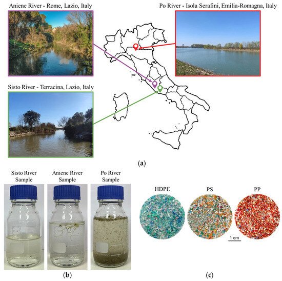
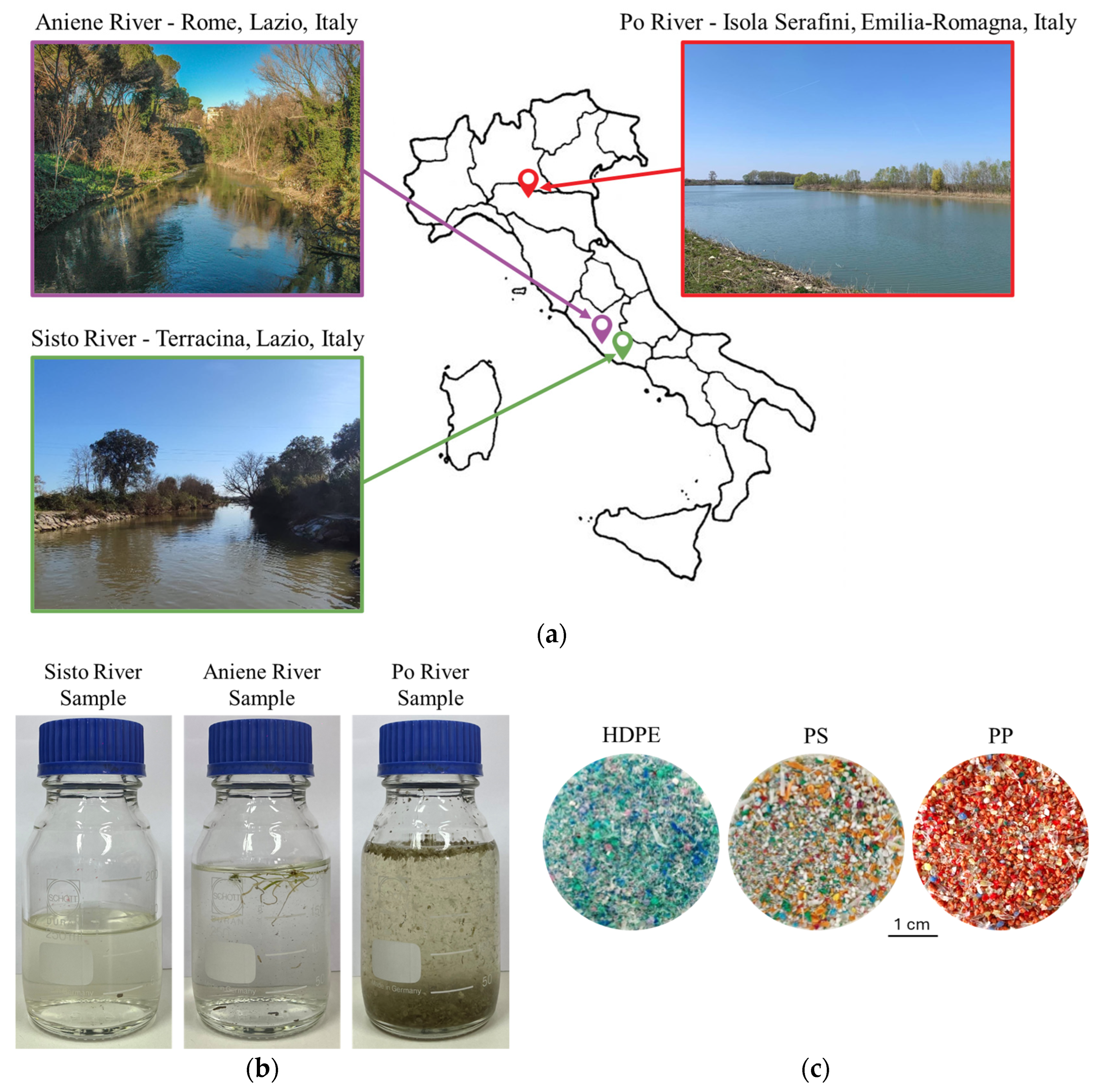
Freshwater samples were collected from three different Italian rivers, i.e., Sisto, Aniene and Po (Figure 1a,b), to provide increasing levels of spectral complexity associated with suspended natural materials. These materials were heterogeneous in composition and variable in abundance, including biogenic debris such as algae, plant residues, and other naturally occurring particulates typical of riverine systems. Samples were stored in glass jars (Schott AG, Mainz, Germany) at +4 °C until laboratory analysis in order to minimize physicochemical alterations prior to HSI acquisition. Prior to MP addition, the freshwater samples were preliminarily visually inspected by stereomicroscopy (Leica Microsystems GmbH, Wetzlar, Germany) to verify the absence of detectable MP particles under the adopted analytical conditions. No MPs were observed during this preliminary assessment.

Figure 1. (a) Location of the freshwater sampling sites in Italy: Sisto River (green), Aniene River (purple), and Po River (red) and (b) the corresponding freshwater samples stored in laboratory glass bottles prior to spectroscopic analysis. (c) MP particles of HDPE, PS, and PP used in this study.

MP particles were manually added to the freshwater samples to simulate controlled contamination scenarios. The studied MP fragments were obtained from the comminution of post-consumer plastic packaging selected among the most widespread polymers in environment, namely HDPE, PS, and PP (Figure 1c) [33]. These particles exhibited different colors, irregular shapes, and variable surface features, with sizes ranging between 250 μm and 1000 μm, selected based on a previous methodological study [21].

2.2. Hyperspectral Imaging Acquisition

Hyperspectral image acquisitions were carried out at the Raw Materials Laboratory (RawMaLab) of the Department of Chemical Engineering, Materials and Environment of Sapienza University of Rome (Italy) using a pushbroom SISUChema XL^TM Chemical Imaging Workstation (Specim, Spectral Imaging Ltd., Oulu, Finland) equipped with an ImSpector^TM N25E spectrometer (Specim, Spectral Imaging Ltd., Oulu, Finland), operating in the SWIR range (1000–2500 nm), coupled with an MCT camera (320 × 240 pixels). The selected configuration of the device uses a 31 mm lens, covering 5 cm field of view (FOV) with a spatial resolution of 150 μm/pixel, acquiring 256 spectral bands with a spectral sampling per pixel of 6.3 nm, and a scanning speed of 17.35 mm/s. A diffuse line illumination unit, consisting of two quartz halogen lamps, was used. The reflectance calibration of the acquired hypercube was set up by an internal standard reference target. Working distance between the spectrograph lens and the sample was about 30 cm.

Two independent sets of hyperspectral acquisitions were prepared and then combined to build the calibration and validation datasets, including five classes: water, natural materials, HDPE, PS, and PP. The “natural materials” class refers to suspended plant fragments and other naturally occurring components present in the freshwater samples.

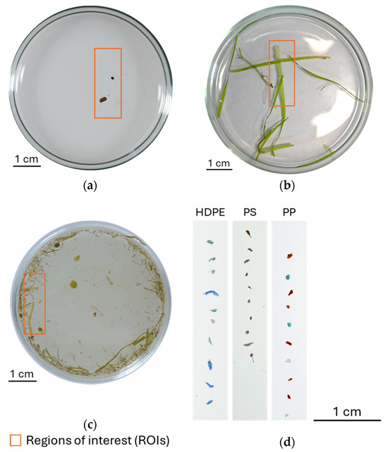
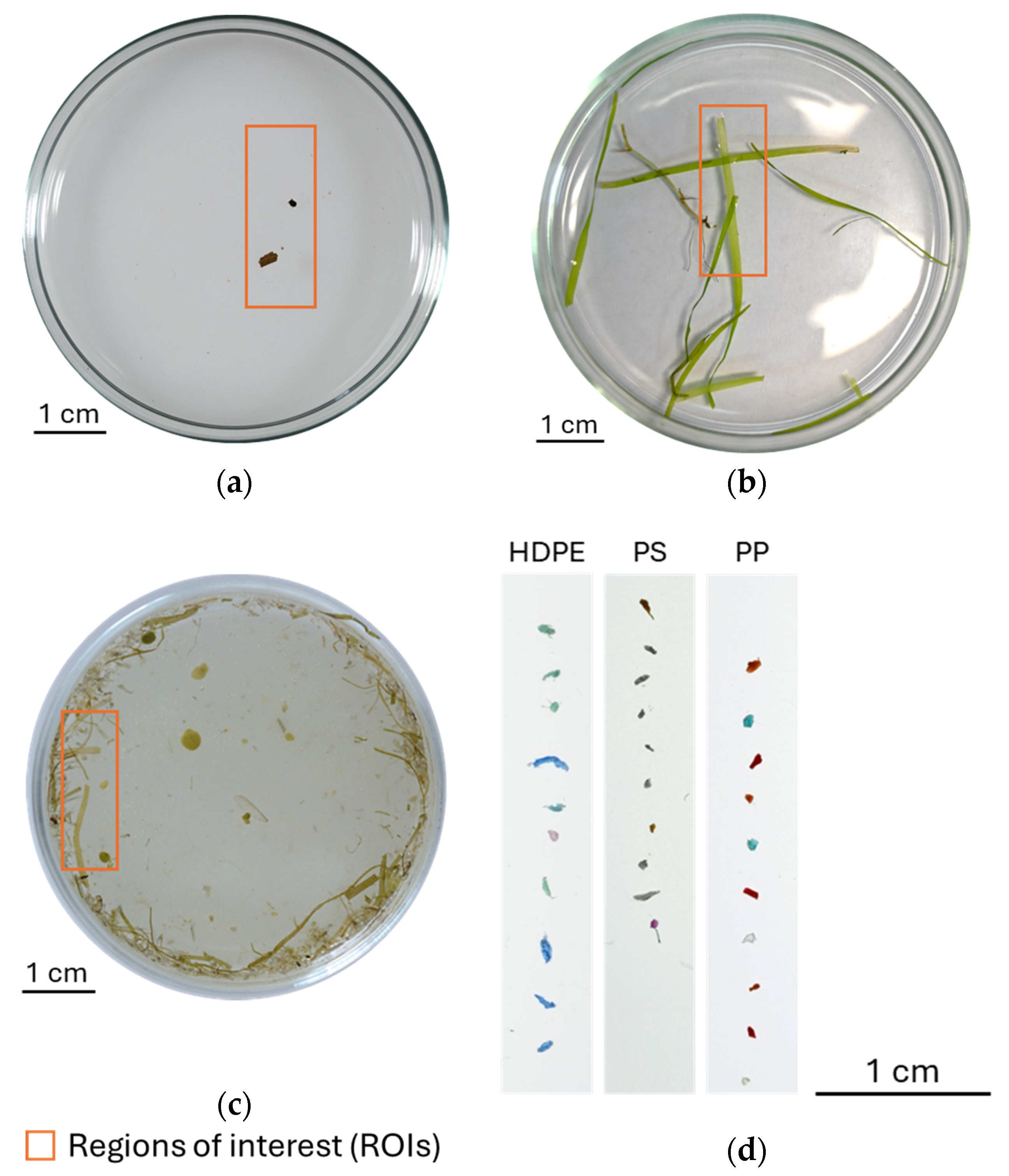
For the calibration dataset, hyperspectral acquisitions were performed on freshwater samples from the three rivers placed in glass Petri dishes (FGH Plus s.r.o., Šumperk, Czech Republic). One hyperspectral image per sample was acquired, capturing both the aqueous matrix and associated natural materials (Figure 2a–c). Regions of interest (ROIs) were selected from these images to build the calibration dataset. In addition, a separate hyperspectral image containing 30 isolated MP particles (10 HDPE, 10 PS, and 10 PP) was acquired under the same experimental conditions and included in the calibration dataset (Figure 2d). The selected particles were characterized by different colors, shapes, sizes (250–1000 μm), and surface characteristics to introduce intra-class variability within each polymer type while maintaining a manageable proof-of-concept experimental design. This dataset design enabled the construction of a representative pixel-wise spectral library including both environmental matrix components and target polymers.

Figure 2. Digital image of glass Petri dishes containing freshwater samples collected from (a) Sisto, (b) Aniene, and (c) Po rivers, characterized by the presence of suspended plant fragments (labelled as “natural materials” class). Orange boxes indicate the regions of interest (ROIs) acquired by HSI and used as calibration dataset containing natural materials and water. (d) Digital image of MP samples (HDPE, PS, and PP) included in the calibration dataset.

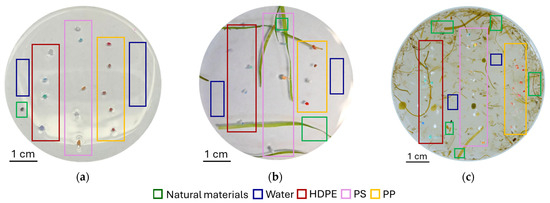
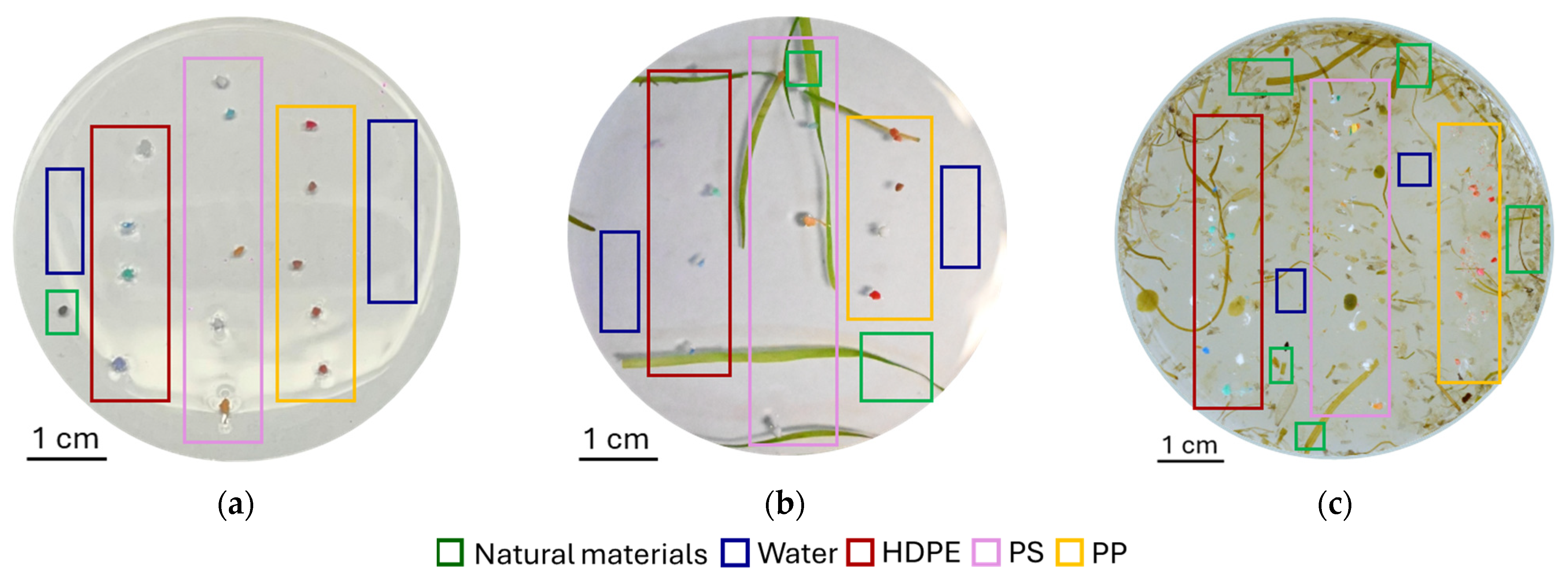
For the validation dataset, hyperspectral acquisitions were performed on independent freshwater samples from the same rivers. MP particles (HDPE, PS, and PP) were added to the samples, simulating environmental contamination scenarios, and one hyperspectral image per sample was acquired (Figure 3).

Figure 3. Digital images of glass Petri dishes containing freshwater samples collected from (a) Sisto, (b) Aniene, and (c) Po rivers, used as validation dataset. The samples are characterized by the presence of suspended natural materials and manually added MPs (HDPE, PS, and PP) to simulate environmental contamination.

2.3. Data Processing and Classification Model Building

Hyperspectral data processing, chemometric preprocessing, exploratory analysis, and classification model building were performed using the MIA Toolbox (version 3.1, Eigenvector Research Inc., Wenatchee, Washington, DC, USA) and the PLS Toolbox (version 9.3, Eigenvector Research Inc., Wenatchee, Washington, DC, USA) within MATLAB^® environment (version 9.12-R2024b, The MathWorks Inc., Natick, MA, USA).

Hyperspectral mosaics were generated for both the calibration and validation datasets. The calibration dataset was built from ROIs selected from freshwater samples (water and natural materials) and from hyperspectral images of individual MP particles (HDPE, PS, and PP), as illustrated in Figure 2. In contrast, the validation dataset consisted of hyperspectral mosaic image generated from freshwater samples different from those used for the calibration dataset, containing natural materials, and added MP particles (HDPE, PS, and PP), as shown in Figure 3.

Subsequently, noisy spectral regions at the beginning and end of the spectra in all datasets were removed, reducing the number of wavelengths from 256 to 240, while preserving the spectral range between 1000 nm and 2500 nm. Spectral preprocessing was then applied to enhance data quality, using commonly adopted algorithms in NIR/SWIR spectroscopy [34,35]. In particular, the following preprocessing algorithms were applied:

• Standard Normal Variate (SNV), to reduce light scattering effects. This method consists of centering each spectrum by subtracting its mean and scaling it by its standard deviation, thereby reducing multiplicative and additive effects [23].
• Smoothing, to attenuate high-frequency noise. This method assumes that adjacent variables in the data matrix (i.e., adjacent columns) are correlated and can be averaged to reduce noise without significant loss of the signal of interest. The degree of smoothing depends on the selected window size and polynomial order [34].
• Gap Segment 1st Derivative, to attenuate additive and multiplicative effects and enhance spectral features. This method computes derivatives between segments of data by a defined gap. The filter is defined by the derivative order, segment size (number of variables per window), and gap size (number of variables between windows) [36].
• Mean Center, to standardize variables prior to multivariate analysis. This step consists of subtracting the mean of each variable, thereby centering the dataset around zero. This preprocessing step removes offsets among variables and allows subsequent multivariate analysis methods (e.g., principal component analysis—PCA and PLS-DA) to focus on variance-related information rather than absolute intensity differences [34].

Following preprocessing, PCA was applied for exploratory analysis to assess spectral variability among the studied classes (i.e., natural materials, water, HDPE, PS, and PP). PCA is a technique capable of reducing high-dimensional data into a limited number of variables, called principal components (PCs), which capture the differences and similarities among the investigated samples [37]. More specifically, PCA score plots were used to visualize the distribution of samples (i.e., pixels) and identify groupings in the reduced multivariate space, whereas PCA loading plots were used to determine the spectral variables (i.e., wavelengths) that most strongly contributed to the variability.

Based on PCA results, a hierarchical classification approach based on partial least square-discriminant analysis (Hi-PLS-DA) was implemented to identify polymer types (i.e., HDPE, PS, and PP) within freshwater matrices. The hierarchical approach represents an efficient strategy for handling complex spectral datasets such as those considered in this study. Its dendrogram-based structure enables a stepwise classification process, while its inherent modularity allows the model to be flexibly adapted and optimized for specific classification tasks [38,39,40]. Accordingly, each node within the hierarchical classifier is implemented as an individual PLS-DA model.

PLS-DA is a linear classification method that is particularly useful for addressing issues of multi-collinearity among variables. It reduces the dimensionality of the original data matrix (X) by projecting it onto a set of latent variables (LVs), maximizing the covariance between the predictor variables (X) and the response variables (Y). The extent of dimensionality reduction is determined by the number of significant LVs. Selection of the appropriate number of LVs is essential to balance the model’s ability and predictive ability [41]. To select an appropriate number of LVs and to reduce overfitting, each PLS-DA model was cross-validated using the Venetian Blind method with a window of 10 split [42].

The Hi-PLS-DA classification model was developed to identify five target classes, i.e., natural materials, water, HDPE, PS, and PP, along with a Not Classified (NC) class, assigned when samples do not belong to any of the predefined classes. This condition typically occurs when the Q residuals or Hotelling T² statistics exceeds the predefined assigned threshold values [43].

2.4. Performance Evaluation

Model performance was assessed by comparing ground truth class maps with class predicted probability maps [41]. Furthermore, pixel-level statistical parameters (i.e., sensitivity and specificity) were used to evaluate classification performance.

To ensure statistical consistency, class populations of all datasets were balanced by randomly selecting the same number of pixels for each class, based on the least represented class. The statistical performances of the classifiers in terms of sensitivity and specificity were evaluated in the calibration, cross-validation, and prediction phases. Pixel-based performance statistics for the calibration and cross-validation phases were obtained from the calibration mosaic dataset, whereas prediction results were obtained from the external validation mosaic dataset. In the prediction phase, additional performance metrics, namely precision and F1-score, were also considered. Equation (1) defines the sensitivity that assesses the model’s ability to correctly identify true positive cases in proportion to all actual positive cases, whereas Equation (2) defines the specificity that assesses the model’s ability to correctly identify true negative cases in proportion to all actual negative cases [44]. Precision (Equation (3)) represents the proportion of correctly classified positive samples among all samples predicted as positive, including both true positives and false positives [28]. F1-score (Equation (4)) combines precision and sensitivity through their harmonic mean, providing a balanced and comprehensive assessment of classification performance [23]. All statistical parameters range from 0 to 1, where 1 corresponds to the ideal value.

$$\mathrm{S}\mathrm{e}\mathrm{n}\mathrm{s}\mathrm{i}\mathrm{t}\mathrm{i}\mathrm{v}\mathrm{i}\mathrm{t}\mathrm{y}={\displaystyle \frac{\mathrm{T}\mathrm{r}\mathrm{u}\mathrm{e} \mathrm{P}\mathrm{o}\mathrm{s}\mathrm{i}\mathrm{t}\mathrm{i}\mathrm{v}\mathrm{e}\mathrm{s}}{\mathrm{T}\mathrm{r}\mathrm{u}\mathrm{e} \mathrm{P}\mathrm{o}\mathrm{s}\mathrm{i}\mathrm{t}\mathrm{i}\mathrm{v}\mathrm{e}\mathrm{s}+\mathrm{F}\mathrm{a}\mathrm{l}\mathrm{s}\mathrm{e} \mathrm{N}\mathrm{e}\mathrm{g}\mathrm{a}\mathrm{t}\mathrm{i}\mathrm{v}\mathrm{e}\mathrm{s}}}$$

(1)

$$\mathrm{S}\mathrm{p}\mathrm{e}\mathrm{c}\mathrm{i}\mathrm{f}\mathrm{i}\mathrm{c}\mathrm{i}\mathrm{t}\mathrm{y}={\displaystyle \frac{\mathrm{T}\mathrm{r}\mathrm{u}\mathrm{e} \mathrm{N}\mathrm{e}\mathrm{g}\mathrm{a}\mathrm{t}\mathrm{i}\mathrm{v}\mathrm{e}\mathrm{s}}{\mathrm{T}\mathrm{r}\mathrm{u}\mathrm{e} \mathrm{N}\mathrm{e}\mathrm{g}\mathrm{a}\mathrm{t}\mathrm{i}\mathrm{v}\mathrm{e}\mathrm{s}+\mathrm{F}\mathrm{a}\mathrm{l}\mathrm{s}\mathrm{e} \mathrm{P}\mathrm{o}\mathrm{s}\mathrm{i}\mathrm{t}\mathrm{i}\mathrm{v}\mathrm{e}\mathrm{s}}}$$

(2)

$$\mathrm{P}\mathrm{r}\mathrm{e}\mathrm{c}\mathrm{i}\mathrm{s}\mathrm{i}\mathrm{o}\mathrm{n}={\displaystyle \frac{\mathrm{T}\mathrm{r}\mathrm{u}\mathrm{e} \mathrm{P}\mathrm{o}\mathrm{s}\mathrm{i}\mathrm{t}\mathrm{i}\mathrm{v}\mathrm{e}\mathrm{s}}{\mathrm{T}\mathrm{r}\mathrm{u}\mathrm{e} \mathrm{P}\mathrm{o}\mathrm{s}\mathrm{i}\mathrm{t}\mathrm{i}\mathrm{v}\mathrm{e}\mathrm{s}+\mathrm{F}\mathrm{a}\mathrm{l}\mathrm{s}\mathrm{e} \mathrm{P}\mathrm{o}\mathrm{s}\mathrm{i}\mathrm{t}\mathrm{i}\mathrm{v}\mathrm{e}\mathrm{s}}}$$

(3)

$$\mathrm{F}1-\mathrm{s}\mathrm{c}\mathrm{o}\mathrm{r}\mathrm{e}={\displaystyle \frac{2\times \mathrm{P}\mathrm{r}\mathrm{e}\mathrm{c}\mathrm{i}\mathrm{s}\mathrm{i}\mathrm{o}\mathrm{n}\times \mathrm{S}\mathrm{e}\mathrm{n}\mathrm{s}\mathrm{i}\mathrm{t}\mathrm{i}\mathrm{v}\mathrm{i}\mathrm{t}\mathrm{y}}{\mathrm{P}\mathrm{r}\mathrm{e}\mathrm{c}\mathrm{i}\mathrm{s}\mathrm{i}\mathrm{o}\mathrm{n}+\mathrm{S}\mathrm{e}\mathrm{n}\mathrm{s}\mathrm{i}\mathrm{t}\mathrm{i}\mathrm{v}\mathrm{i}\mathrm{t}\mathrm{y}}}$$

(4)

3. Results

3.1. Average Reflectance Spectra and Exploration Analysis Results

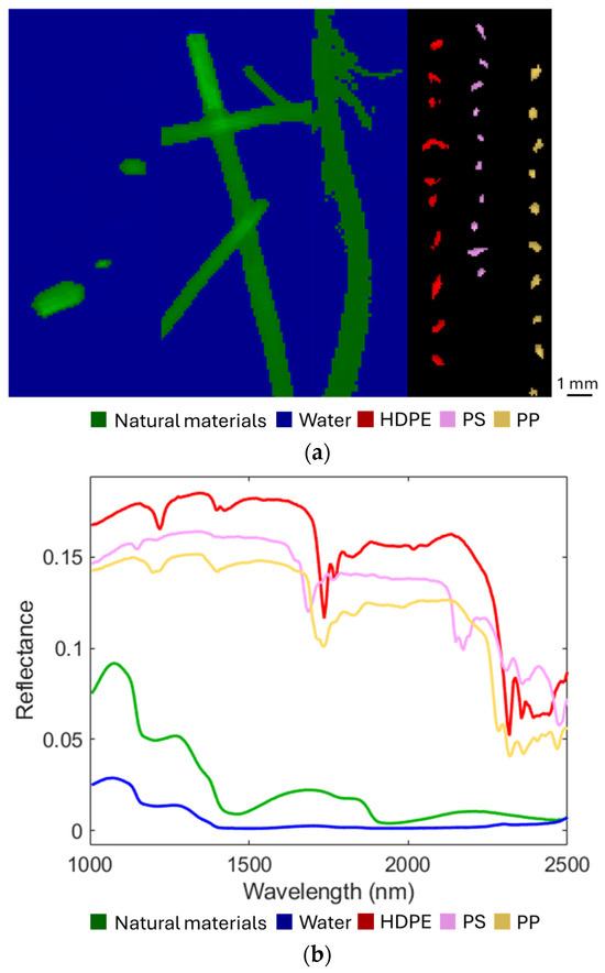
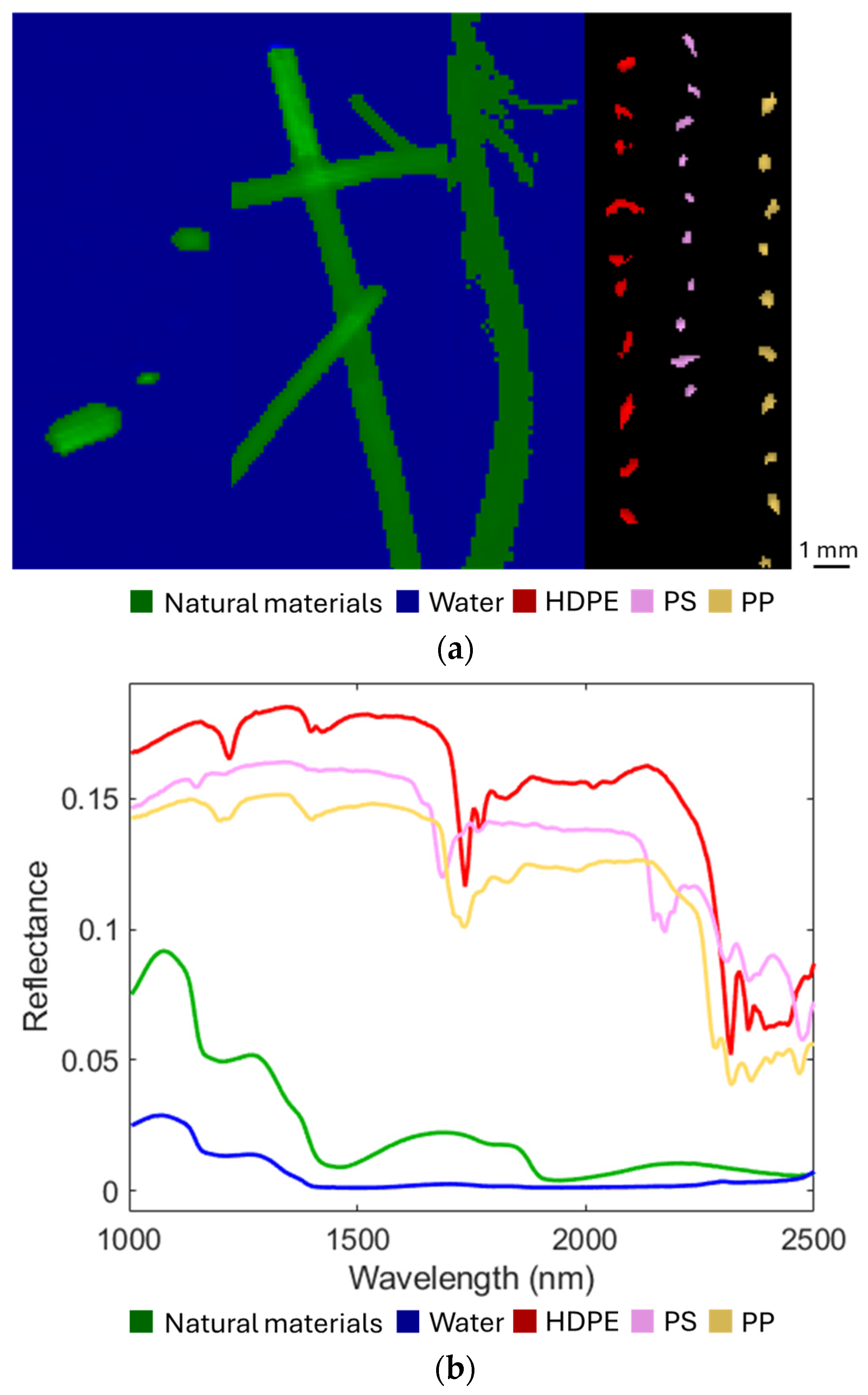
Figure 4a shows the hyperspectral mosaic used as calibration dataset (the corresponding source images are reported in Figure 2), comprising a total of 18,033 pixels distributed as follows: 2457 pixels for natural materials, 15,059 for water, 220 for HDPE, 121 for PS, and 176 for PP. Figure 4b reports the corresponding average raw reflectance spectra of each investigated class. The analysis of these spectra highlights the most significant SWIR regions useful for the characterization of the investigated classes.

Figure 4. (a) Calibration dataset showing the studied classes: natural materials, water, HDPE, PS and PP; (b) average raw reflectance spectra of the investigated classes in the SWIR range.

The reflectance spectrum of the natural materials class (green line), mainly consisting of leaves, algae, and other vegetal components, is characterized by absorption features observed around 1200 nm, and more prominently in the regions 1400–1500 nm and 1900–2000 nm. These features are mainly associated with O-H vibrations, reflecting the combined contribution of the vegetal components and the surrounding aqueous matrix [45]. Water (blue line) reflectance spectrum is characterized by absorption bands around 1200 nm and 1400 nm, followed by a relatively flat spectral profile at low reflectance levels, resulting from strong and broad absorption bands up to 2500 nm [46]. MP reflectance spectra show complex and structured profiles, with distinct absorption features for each polymer type (HDPE, PS and PP) in the SWIR range, contributing to their differentiation [47,48,49]. HDPE (red line) is characterized by a sharp band at 1210 nm which can be assigned to the C-H stretching of second overtone region, along with two bands around 1390 nm and 1420 nm related to the combination of C-H stretching in the second overtone region. The absorptions at 1730 and 1750 nm are related to C-H and C-H₂ in the first overtone region. PS (pink line) spectrum is characterized by one band at 1140 nm related to the C-H₃ stretching of second overtone region, 1210 nm band C-H stretching of second overtone region, 1700 nm band related to aromatic C-H stretch in the first overtone and three peaks assigned to aromatic C-H combination region (2100, 2150 and 2200 nm). PP (yellow line) spectrum shows two absorptions (1210 and 1220 nm) of C-H stretching in the second overtone region, peak at 1420 nm assigned to the C-H combination in the second overtone region, and asymmetric C-H stretch of first overtone (1700 and 1730 nm). All the three-polymer types show various bands in the first combination region related to C-H and C=O (2200–2500 nm).

The results obtained for the different preprocessing combinations and the corresponding PCA, selected for the definition of the Hi-PLS-DA rules, are presented and discussed in the following.

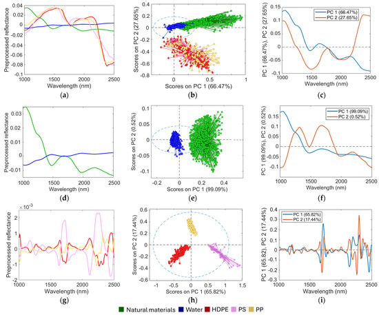
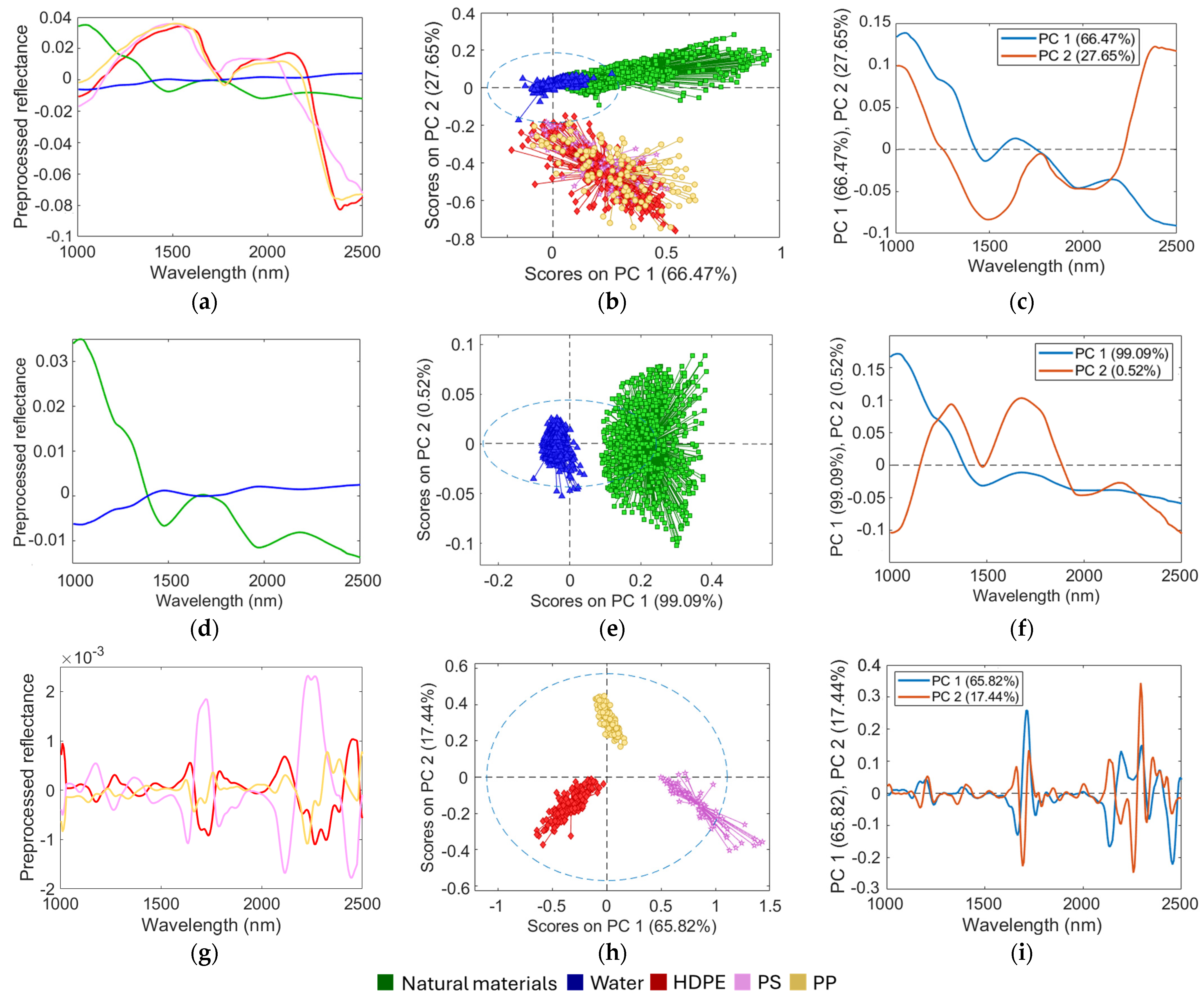
Rule 1: The preprocessed spectra (Figure 5a) were obtained after application of SNV (scale offset = 1.00), Smoothing (window: 25 pt), and Mean Center algorithms. The PCA score plot (Figure 5b) indicated that the first two PCs accounted for most of the data variability, with PC1 and PC2 explaining 66.47% and 27.65% of the total variance, respectively. The score plot highlighted the presence of two well-defined clusters: natural materials + water mainly distributed in the PC1 and PC2 positive values and HDPE + PS + PP mainly distributed in the PC1 positive and PC2 negative values. The loading plot (Figure 5c) shows that the main contribution for the definition of PC1 comes from positive values of the 1000–1450 nm region and negative values from 1550 to 2000 nm. The highest contribution for the definition of PC2 comes from positive values of 1000–1300 nm and 2200–2500 nm regions, and negative values between 1750 and 2300 nm.

Figure 5. Data processing and PCA results. Rule 1: (a) preprocessed reflectance spectra, (b) PCA score plot, (c) loading plot; Rule 2: (d) preprocessed reflectance spectra, (e) PCA score plot, (f) loading plot; Rule 3: (g) preprocessed reflectance spectra, (h) PCA score plot, (i) loading plot.

Rule 2: The preprocessed spectra (Figure 5d) were obtained after application of SNV (scale offset = 1.00), Smoothing (window: 25 pt), and Mean Center algorithms. The PCA score plot (Figure 5e) showed that the majority of the variance contained in the dataset was described by the first two PCs, where PC1 and PC2 explained 99.09% and 0.52% of the total variance, respectively. The score plot revealed a clear separation between two distinct clusters: natural materials class was located in the positive quadrant of PC1, while water was distributed in the negative values of PC1. The loading plot (Figure 5f) confirms that the main discriminant components are located around 1000 nm and 1200 nm and in the region between 1500 nm and 2000 nm. PC1 is predominantly characterized by positive values in the 1000–1300 nm range and negative values from around 1400 nm to 2500 nm. In contrast, PC2 exhibits alternating positive and negative contributions, with positive peaks around 1300 nm and 1700 nm and negative values near 1000 nm and above 2000 nm. This pattern indicates that PC2 captures the variance associated with natural materials, whose spectral response differs from water, with the sign of the loadings highlighting opposing contributions between the two components.

Rule 3: The preprocessed spectra (Figure 5g) were obtained after application of SNV, Gap Segment 1st Derivative (gap: 3, segment: 3), and Mean Center algorithms. The PCA score plot (Figure 5h) indicated that the first two PCs explained most of the data variability, accounting for 65.82% and 17.44% of the total variance for PC1 and PC2, respectively. The score plot showed a distinct separation between three main clusters: HDPE mainly distributed in the negative quadrants of PC1 and PC2, PS was located in the PC1 positive and PC2 negative values, while PP was situated along the zero axis of PC1 and in the positive values of PC2. The loading plot (Figure 5i) shows that the region around 1700 nm allows the three polymers (HDPE, PS, and PP) to be distinguished from one another. The region between 2000 and 2500 nm is also crucial for distinguishing between the different spectral features of these polymers.

The results obtained from this exploratory analysis suggest the potential for exploiting a hierarchical classification structure based on the progressive spectral separability of the different classes, with the aim of preserving polymer-related information while mitigating the influence of the surrounding matrix.

3.2. Hi-PLS-DA Model Structure

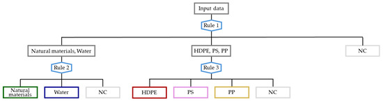
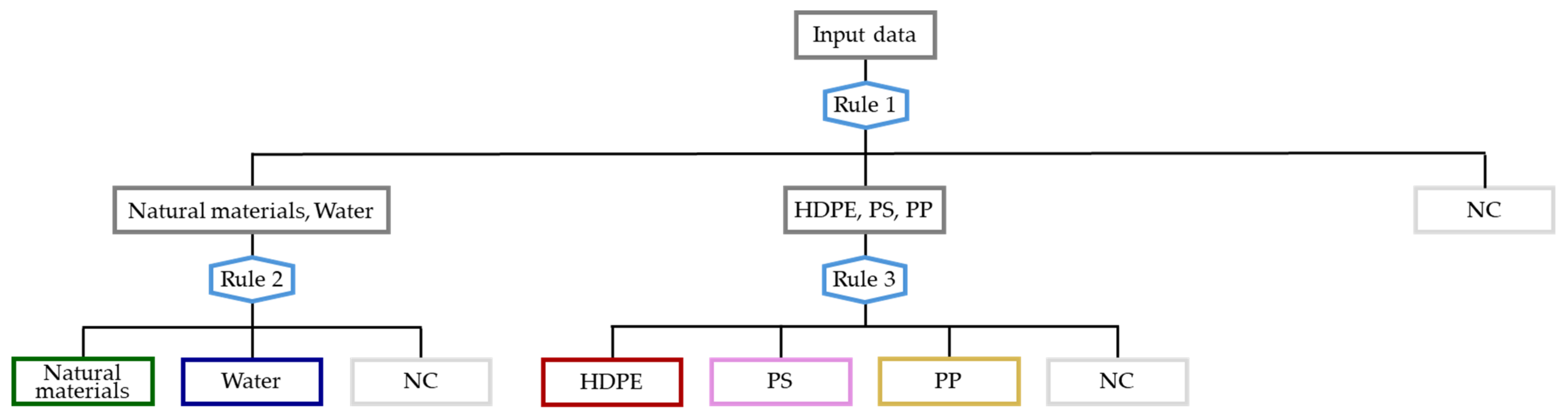
Based on the patterns identified through PCA, a hierarchical classification structure, composed of three sequential decision rules, each implemented as an individual PLS-DA model, was defined. Table 1 summarizes, for each rule, the corresponding preprocessing strategies, number of LVs, and classification outputs adopted in the Hi-PLS-DA model. Figure 6 illustrates the hierarchical classification structure.

Table 1. Summary of the Hi-PLS-DA classification scheme, including preprocessing strategies, number of LVs, and classification output for each rule.

Rules	Preprocessing Strategy	LVs	Classification Target Output
Rule 1	SNV (scale offset = 1.00) + Smoothing (window: 25 pt) + Mean Center	2	Natural materials + Water vs. HDPE + PS + PP
Rule 2	SNV (scale offset = 1.00) + Smoothing (window: 25 pt) + Mean Center	4	Natural materials vs. Water
Rule 3	SNV + Gap Segment 1st Derivative (gap: 3, segment: 3) + Mean Center	3	HDPE vs. PS vs. PP

Figure 6. Dendrogram-based structure of the Hi-PLS-DA model used to classify the five studied classes (i.e., natural materials, water, HDPE, PS, and PP). Additional NC class = not classified class.

Rule 1 provided a classification output distinguishing non-MP classes (natural materials and water) from MP classes (HDPE, PS, and PP). Rule 2 refined the classification by discriminating between natural materials and water, while Rule 3 further resolved the MP classes by distinguishing HDPE, PS, and PP.

3.3. Classification Results

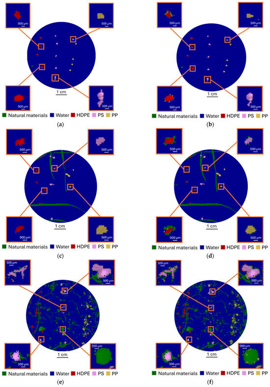
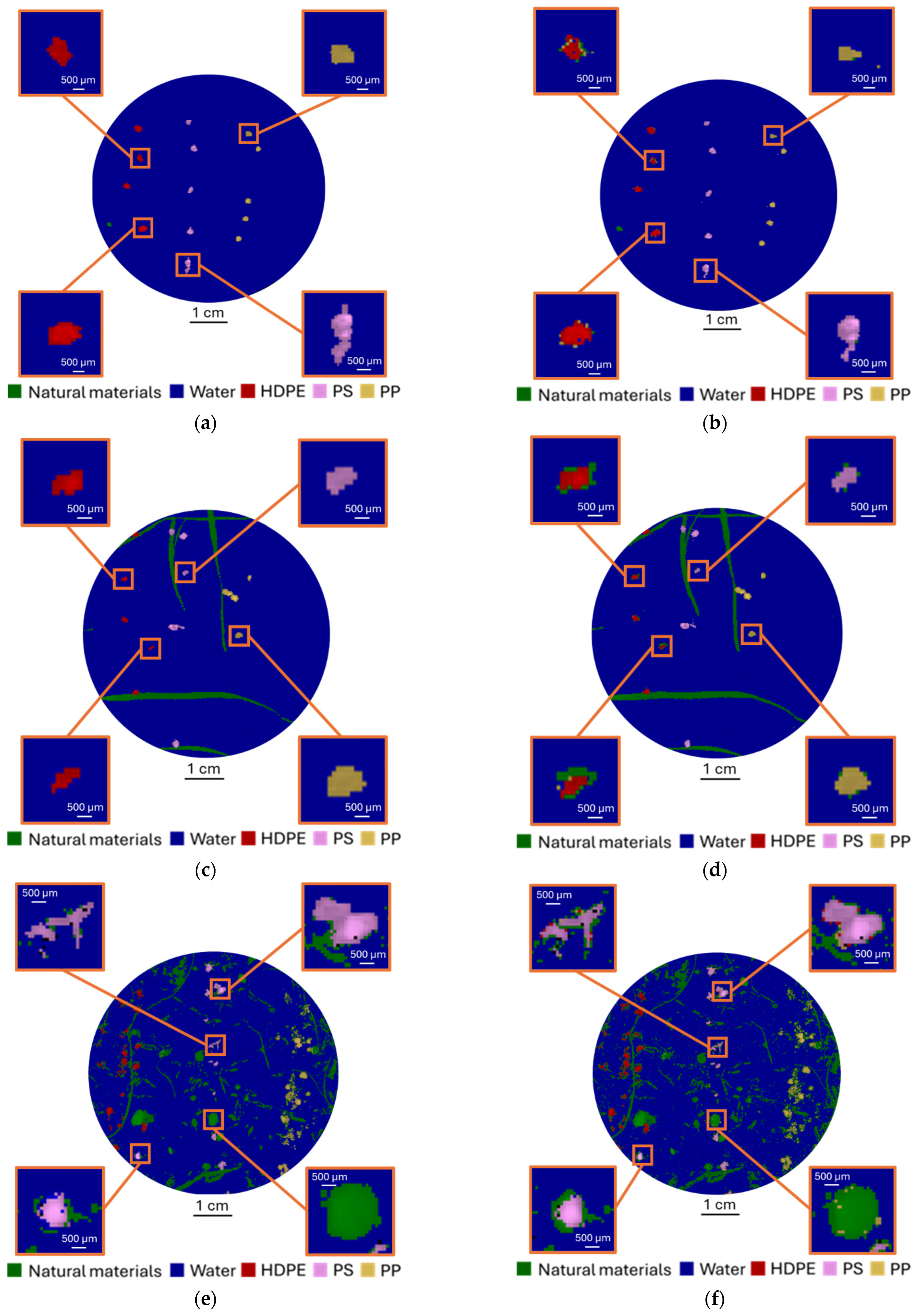
Figure 7a–f shows the classification results obtained for the validation mosaic dataset. For visualization purposes, the results are presented as individual images, one for each considered freshwater matrix, to better illustrate the classification outcomes and support a more comprehensive interpretation of the image-based prediction results. For each hyperspectral image, the ground truth class map (Figure 7a,c,e) and the corresponding Hi-PLS-DA predicted class map (Figure 7b,d,f) are shown. A direct visual comparison between the ground truth and predicted maps indicates that the model was not only able to correctly identify the presence of suspended MPs in the aqueous matrix, but also to discriminate between different types of polymers (i.e., HDPE, PS, and PP). In addition to polymer discrimination, the model also shows consistent performance in identifying the natural materials class across the freshwater samples. The prediction maps of the validation dataset correctly show the gradient of matrix complexity observed among the analyzed samples, ranging from low in the Sisto River to moderate in the Aniene River and high in the Po River. Despite this overall agreement, some localized classification errors can be observed. For the Sisto (Figure 7a,b) and Aniene images (Figure 7c,d), the results show limited misclassifications, mainly at the edges of MP particles. These effects can be attributed to boundary conditions, where individual pixels include spectral contributions from both the polymer and the surrounding matrix due to the limited spatial resolution (150 µm/pixel), resulting in spectral mixing and reduced accuracy in class attribution. In addition, the presence of water introduces strong absorption features that can attenuate and partially mask the spectral signature of polymers, further reducing their discriminability. Furthermore, prediction results for the Po sample, representing the most complex case in terms of both the abundance and variability of natural materials as well as the higher number of MP particles, reveal a higher number of misclassified pixels compared to the Sisto and Aniene samples. This increased heterogeneity of the matrix, including mucilage-like components, amplifies spectral interference and reduces class separability. To better understand the model’s performance, some cases of misclassification have been enlarged and highlighted in orange boxes.

Figure 7. Hi-PLS-DA results for the validation mosaic dataset, displayed as individual images according to freshwater matrix for visualization purposes: (a) ground truth and (b) predicted maps for Sisto; (c) ground truth and (d) predicted maps for Aniene; (e) ground truth and (f) predicted maps for Po. Orange boxes highlight representative classification errors by comparing the ground truth areas with the corresponding predicted areas.

Overall, despite these effects, the model provides reliable identification of MP particles, with consistent pixel-wise class attribution within particle regions and misclassifications mainly confined to boundary areas. This behavior is consistent with the statistical performance of the model, reported in Table 2 and Table 3. In particular, the results obtained in calibration and cross-validation indicate high performance, with sensitivity and specificity values ranging from 0.926 to 1.000 (Table 2). Rule 1 exhibits excellent performance, with both sensitivity and specificity exceeding 0.992 in calibration and cross-validation, confirming the robustness of the model in discriminating between the freshwater matrix containing suspended natural materials and the polymer classes (HDPE, PS, and PP).

Table 2. Statistical parameters (sensitivity and specificity) in calibration (Cal) and cross-validation (CV) phases for each rule of the Hi-PLS-DA.

Rules	Classes	Sensitivity (Cal)	Specificity (Cal)	Sensitivity (CV)	Specificity (CV)
Rule 1	Natural materials + Water	1.000	0.992	1.000	0.992
	HDPE + PS + PP	0.992	1.000	0.992	1.000
Rule 2	Natural materials	0.999	0.926	0.999	0.926
	Water	0.926	0.999	0.926	0.999
Rule 3	HDPE	1.000	1.000	1.000	1.000
	PS	1.000	1.000	1.000	1.000
	PP	1.000	1.000	1.000	1.000

Table 3. Statistical parameters (sensitivity, specificity, precision and F1-score) in prediction (Pred) phase for each class of the Hi-PLS-DA.

Classes	Sensitivity (Pred)	Specificity (Pred)	Precision (Pred)	F1-Score (Pred)
Natural materials	0.977	0.982	0.931	0.953
Water	0.980	0.973	0.900	0.938
HDPE	0.970	0.998	0.991	0.980
PS	0.934	0.999	0.997	0.964
PP	0.930	0.996	0.984	0.956

Rule 2 shows strong performance in discriminating between natural materials and water, with sensitivity and specificity values consistently above 0.926. Finally, Rule 3 achieves very high classification performance in distinguishing among the three polymer types (HDPE, PS, and PP), with both sensitivity and specificity equal to 1.000 in calibration and cross-validation.

The statistical parameters in the prediction phase (Table 3), calculated using the balanced validation mosaic dataset (1320 pixels per class, corresponding to the least represented class, i.e., PS), range from 0.900 to 0.999, indicating overall satisfactory predictive performance.

This pattern is consistent with the limited misclassifications observed in the prediction maps, mainly located at particle boundaries, and supports the reliability of the hierarchical classification approach. For completeness, the confusion matrix corresponding to the balanced validation mosaic dataset is reported in the Supplementary Materials (Table S1), together with the confusion matrices obtained from the Sisto, Aniene, and Po River subsets (Tables S2–S4), which reflect the naturally unbalanced class distributions observed in the freshwater samples.

4. Discussion

The results obtained in this study demonstrate that the proposed SWIR-HSI-based workflow, combined with chemometrics and hierarchical modeling, enables the direct identification of suspended MPs in freshwater samples without preliminary sample pretreatment or manual particle isolation, even in the presence of complex environmental matrices. Unlike conventional analytical procedures, which typically rely on filtration, density separation, organic matter removal, and manual particle selection, the proposed approach operates directly on untreated freshwater samples, preserving matrix heterogeneity while avoiding any preliminary isolation steps.

Building upon previous studies such as Gebejes et al. [31], which demonstrated the feasibility of direct identification of MPs in tap water samples under controlled conditions by HSI, the present work extends this approach using real freshwater samples containing natural materials from three Italian rivers. This introduces additional matrix complexity and provides a representative description of environmental conditions. Moreover, the MPs investigated in this study were obtained from the comminution of post-consumer plastic packaging, thereby introducing variability in composition, additives, and surface properties, thus better reflecting real-world contaminated river scenarios.

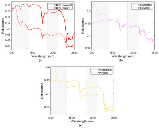
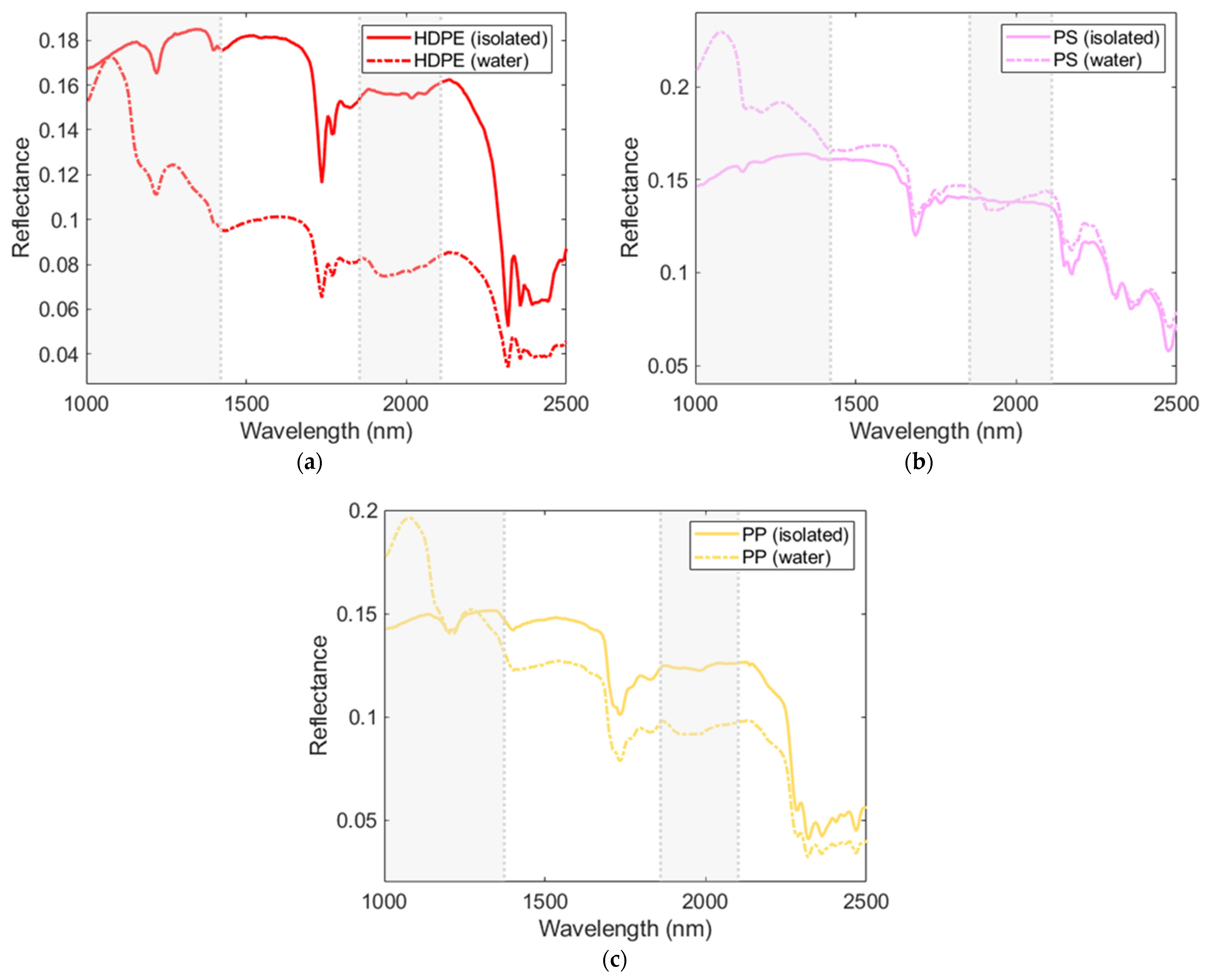
Consistently with previous observations [23,31], the presence of the aqueous matrix can affect the spectral response of MPs, leading to modifications of spectral profiles and partial overlap with additional spectral contributions. In particular, the comparison between the average reflectance spectra obtained from the calibration dataset (isolated MPs) and the validation dataset (MPs in freshwater) highlights aqueous matrix-induced effects on the polymer spectrum, mainly in the 1000–1400 nm and 1810–2090 nm regions (highlighted by grey areas in Figure 8). Despite these challenges, MP particles were generally correctly identified, indicating that the proposed hierarchical classification strategy effectively supports their detection under these complex conditions. By decomposing the classification problem into sequential decision steps, the Hi-PLS-DA framework enables progressive discrimination among spectral classes, reducing matrix-related interference. The spectral mixing and partial masking effects are particularly evident only at particle boundaries, where contributions from adjacent classes may lead to confusion both among different MPs and between MPs and surrounding matrix components (including natural materials). This approach is consistent with previous studies demonstrating that structured or hierarchical modeling can improve robustness in complex multiclass problems [38,39,40].

Figure 8. SWIR average reflectance spectra of (a) HDPE, (b) PS, and (c) PP acquired as isolated particles (calibration dataset) and under aqueous conditions (validation dataset). Grey shaded areas highlight spectral regions (1000–1400 nm and 1850–2100 nm) where differences between isolated and aqueous conditions are more evident.

At the same time, it should be noted that real environmental MPs exhibit substantially greater heterogeneity than the particles investigated in this study. In addition to a broader variety of polymer types and blends, variable pigmentation, irregular shapes, and a wider particle size distribution, environmental MPs may undergo photo-oxidation, mechanical abrasion, biofilm formation, and adsorption of organic and inorganic contaminants. These factors may increase spectral complexity and further challenge polymer identification. In particular, smaller particles, potentially approaching or below the instrumental limit of detection, may not be reliably resolved. Furthermore, as observed in more complex samples (e.g., Po River), particle aggregation can occur, hindering the clear delineation of individual particle boundaries and complicating the interpretation of quantification results. Within these constraints, the present proof-of-concept study provides preliminary evidence supporting the feasibility of direct MP identification in untreated freshwater matrices using SWIR-HSI. In the investigated samples and under controlled conditions, the characteristic absorption bands of the polymer matrix remained sufficiently detectable to enable satisfactory MP classification despite the presence of freshwater matrix interferences (Figure 8). The proposed workflow, based on direct analysis of untreated samples, eliminates the need for preliminary sample pretreatment and manual particle isolation, thereby reducing sample handling and eliminating time-consuming preprocessing steps, with a consequent simplification of the overall analytical workflow. This feature may represent an advantage for future environmental monitoring applications, where rapid, operationally simple, and more sustainable analytical strategies are desirable. In this context, the approach is aligned with the SDGs, in particular SDG9, SDG14, and SDG15, supporting the development of analytical strategies with lower resource consumption and reduced environmental impact [32].

5. Conclusions

This proof-of-concept study investigated the potential of SWIR-HSI combined with a hierarchical chemometric approach for the direct identification of selected MPs spiked into freshwater samples under controlled conditions and characterized by the presence of suspended natural materials.

The results demonstrate that the proposed workflow enables the discrimination of different polymer types (HDPE, PS, and PP) in complex and heterogeneous matrices, supporting the feasibility of MP identification without preliminary sample treatment. At the same time, some limitations were observed. In particular, classification errors at particle boundaries highlight the influence of spectral mixing, water-induced signal modifications, and matrix heterogeneity. Despite these effects, sufficient spectral variability is preserved to allow class discrimination through the classification model. Although obtained within a laboratory-scale methodological framework, these results provide useful insights for the development of rapid and environmentally sustainable analytical approaches for MP identification in complex freshwater matrices with minimal sample preparation requirements. Further developments are required to extend the applicability of the approach to more complex and representative environmental scenarios, including the detection of smaller particles than those investigated in this study (i.e., below 250 μm), the inclusion of a wider range of polymer types and morphologies, environmentally weathered MPs affected by oxidation and biofilm formation, and the assessment of matrix–particle interactions under naturally contaminated conditions.

References

- Uddin, M.; Kormoker, T.; Uddin, M.S.; Idris, A.M.; Ampah, J.D.; Haque, M.K.; Hossain, M.Y.; BakarSiddique, M.A.; Islam, M.S.; Islam, A.R.M.T.; et al. Micro (nano) plastics as emerging pollutants in global aquatic and terrestrial ecosystems: A bibliometric analysis. Environ. Forensics 2025, 26, 58–90. [Google Scholar] [CrossRef] [Scilit]
- Dey, S.; Veerendra, G.T.N.; Babu, P.A.; Manoj, A.P.; Nagarjuna, K. Degradation of plastics waste and its effects on biological ecosystems: A scientific analysis and comprehensive review. Biomed. Mater. Devices 2024, 2, 70–112. [Google Scholar] [CrossRef] [Scilit]
- Thompson, R.C.; Olsen, Y.; Mitchell, R.P.; Davis, A.; Rowland, S.J.; John, A.W.; McGonigle, D.; Russell, A.E. Lost at sea: Where is all the plastic? Science 2004, 304, 838. [Google Scholar] [CrossRef] [Scilit] [PubMed]
- Talreja, N.; Hegde, C.; Kumar, E.M.; Chavali, M. Emerging environmental contaminants: Sources, consequences and future challenges. In Green Technologies for Industrial Contaminants; Wiley: Hoboken, NJ, USA, 2025; pp. 119–149. [Google Scholar] [CrossRef] [Scilit]
- Thompson, R.C.; Courtene-Jones, W.; Boucher, J.; Pahl, S.; Raubenheimer, K.; Koelmans, A.A. Twenty years of microplastic pollution research—What have we learned? Science 2024, 386, eadl2746. [Google Scholar] [CrossRef] [Scilit] [PubMed]
- Vishavjeet, R.; Ahlawat, Y.K.; Singh, R.; Bhardwaj, J.K.; Ajaybeer, K.; Kumar, S.; Sharma, P.; Choudhary, R.; Didwania, N.; Kumar, D.; et al. Microplastics and Health: A Review on Environmental Exposure, Toxicokinetics and Biological Effects. Sustainability 2026, 18, 3527. [Google Scholar] [CrossRef] [Scilit]
- Mokhtar, D.M. Microplastics in Aquatic Ecosystems: Implications for Ecosystem Services and the Sustainability of Fisheries. Sustainability 2026, 18, 3021. [Google Scholar] [CrossRef] [Scilit]
- Duis, K.; Coors, A. Microplastics in the aquatic and terrestrial environment: Sources (with a specific focus on personal care products), fate and effects. Environ. Sci. Eur. 2016, 28, 2. [Google Scholar] [CrossRef] [Scilit] [PubMed]
- Hamidiaala, S.; Babajamaaty, G.; Mohammadian, A.; Pilechi, A.; Ghazizadeh, M. Identification of Microplastic Accumulation Zones in a Tidal River: A Case Study of the Fraser River, British Columbia, Canada. Sustainability 2025, 17, 8591. [Google Scholar] [CrossRef] [Scilit]
- González, D.; Hanke, G.; Tweehuysen, G.; Bellert, B.; Holzhauer, M.; Palatinus, A.; Hohenblum, P.; Oosterbaan, L. Riverine Litter Monitoring—Options and Recommendations; MSFD GES TG Marine Litter Thematic Report; Publications Office of the European Union: Luxembourg, 2016.
- Mekong River Commission. Protocol for Riverine Microplastics Monitoring: A Detailed Methodology for Long-Term and Cost-Effective Monitoring of Riverine Plastic Debris Pollution in the Lower Mekong River; Mekong River Commission Secretariat: Vientiane, Laos, 2024. [Google Scholar]
- Lin, C.T.; Chiu, M.C.; Kuo, M.H. A mini-review of strategies for quantifying anthropogenic activities in microplastic studies in aquatic environments. Polymers 2022, 14, 198. [Google Scholar] [CrossRef] [Scilit] [PubMed]
- United Nations Environment Programme. Monitoring Plastics in Rivers and Lakes: Guidelines for the Harmonization of Methodologies; United Nations Environment Programme: Nairobi, Kenya, 2020. [Google Scholar]
- Rani, M.; Ducoli, S.; Depero, L.E.; Prica, M.; Tubić, A.; Ademovic, Z.; Morrison, L.; Federici, S. A complete guide to extraction methods of microplastics from complex environmental matrices. Molecules 2023, 28, 5710. [Google Scholar] [CrossRef] [Scilit] [PubMed]
- AMAP. AMAP Litter and Microplastics Monitoring Guidelines, Version 1.0; Arctic Monitoring and Assessment Programme (AMAP): Tromsø, Norway, 2021; 257p.
- GESAMP. Guidelines for the Monitoring and Assessment of Plastic Litter and Microplastics in the Ocean; Kershaw, P.J., Turra, A., Galgani, F., Eds.; Rep. Stud. GESAMP No. 99; GESAMP: London, UK, 2019; 130p. [Google Scholar]
- Serranti, S.; Bonifazi, G.; Cocozza, P.; Cucuzza, P.; Palmieri, R.; Benzi, M.; Lezzi, M.; Mazziotti, C.; Riccardi, E.; Barbieri, E.; et al. Comparison of hyperspectral imaging and FTIR spectroscopy for microplastic polymer identification: Proposal of a scalable protocol validated in a 12-month river survey. Talanta 2026, 302, 129361. [Google Scholar] [CrossRef] [Scilit] [PubMed]
- Xu, J.L.; Thomas, K.V.; Luo, Z.; Gowen, A.A. FTIR and Raman imaging for microplastics analysis: State of the art, challenges and prospects. TrAC Trends Anal. Chem. 2019, 119, 115629. [Google Scholar] [CrossRef] [Scilit]
- Mikulec, V.; Adamović, P.; Cvetković, Ž.; Ivešić, M.; Gajdoš Kljusurić, J. Green techniques for detecting microplastics in marine with emphasis on FTIR and NIR spectroscopy—Short review. Processes 2023, 11, 2360. [Google Scholar] [CrossRef] [Scilit]
- Picó, Y.; Barceló, D. Analysis of microplastics and nanoplastics: How green are the methodologies used? Curr. Opin. Green Sustain. Chem. 2021, 31, 100503. [Google Scholar] [CrossRef] [Scilit]
- Serranti, S.; Capobianco, G.; Cucuzza, P.; Bonifazi, G. Efficient microplastic identification by hyperspectral imaging: A comparative study of spatial resolutions, spectral ranges and classification models to define an optimal analytical protocol. Sci. Total Environ. 2024, 954, 176630. [Google Scholar] [CrossRef] [Scilit] [PubMed]
- Serranti, S.; Bonifazi, G.; Capobianco, G.; Gorga, E.; D’Agostini, M.; Dall’Ava, A. Custom hyperspectral imaging scanner for microplastic detection and classification: Hardware and data processing specifications. In Proceedings of the Algorithms, Technologies, and Applications for Multispectral and Hyperspectral Imaging XXXI, Orlando, FL, USA, 13–17 April 2025; SPIE: Bellingham, WA, USA, 2025; Volume 13455, pp. 247–257. [Google Scholar] [CrossRef] [Scilit]
- Kitahashi, T.; Nakajima, R.; Nomaki, H.; Tsuchiya, M.; Yabuki, A.; Yamaguchi, S.; Zhu, C.; Kanaya, Y.; Lindsay, D.J.; Chiba, S.; et al. Development of robust models for rapid classification of microplastic polymer types based on near infrared hyperspectral images. Anal. Methods 2021, 13, 2215–2222. [Google Scholar] [CrossRef] [Scilit] [PubMed]
- de Juan, A.; de Oliveira, R.R. Hyperspectral image and chemometrics. A step beyond classical spectroscopic PAT tools. Anal. Bioanal. Chem. 2026, 418, 23–34. [Google Scholar] [CrossRef] [Scilit] [PubMed]
- Cheng, M.F.; Mukundan, A.; Karmakar, R.; Valappil, M.A.E.; Jouhar, J.; Wang, H.C. Modern trends and recent applications of hyperspectral imaging: A review. Technologies 2025, 13, 170. [Google Scholar] [CrossRef] [Scilit]
- Khort, D.O.; Kutyrev, A.; Smirnov, I.; Andriyanov, N.; Filippov, R.; Chilikin, A.; Astashev, M.E.; Molkova, E.A.; Sarimov, R.M.; Matveeva, T.A.; et al. Enhancing sustainable automated fruit sorting: Hyperspectral analysis and machine learning algorithms. Sustainability 2024, 16, 10084. [Google Scholar] [CrossRef] [Scilit]
- Karlsson, T.M.; Grahn, H.; van Bavel, B.; Geladi, P. Hyperspectral imaging and data analysis for detect-ing and determining plastic contamination in seawater filtrates. J. Near Infrared Spectrosc. 2016, 24, 141–149. [Google Scholar] [CrossRef] [Scilit]
- Shan, J.; Zhao, J.; Liu, L.; Zhang, Y.; Wang, X.; Wu, F. A novel way to rapidly monitor microplastics in soil by hyperspectral imaging technology and chemometrics. Environ. Pollut. 2018, 238, 121–129. [Google Scholar] [CrossRef] [Scilit] [PubMed]
- Rizzo, A.; Serranti, S.; Cucuzza, P.; Lisco, S.; Marsico, A.; Bonifazi, G.; Mastronuzzi, G. Application of hyperspectral imaging and machine learning for the automatic identification of microplastics on sandy beaches. In Proceedings of the Algorithms, Technologies, and Applications for Multispectral and Hyperspectral Imaging XXX, National Harbor, MD, USA, 7 June 2024; SPIE: Bellingham, WA, USA, 2024; Volume 13031, pp. 181–193. [Google Scholar] [CrossRef] [Scilit]
- Seidel, M.; Hutengs, C.; Bauer, J.; Schneider, B.; Ortner, M.; Thiele-Bruhn, S.; Vohland, M. Efficient screening of microplastics in soils using hyperspectral imaging in the short-wave infrared range coupled with machine learning–A laboratory-based experiment. Ecol. Indic. 2025, 173, 113301. [Google Scholar] [CrossRef] [Scilit]
- Gebejes, A.; Hrovat, B.; Semenov, D.; Kanyathare, B.; Itkonen, T.; Keinänen, M.; Koistinen, K.; Peiponen, K.-E.; Roussey, M. Hyperspectral imaging for identification of irregular-shaped microplastics in water. Sci. Total Environ. 2024, 944, 173811. [Google Scholar] [CrossRef] [Scilit] [PubMed]
- United Nations Department of Economic and Social Affairs Sustainable Development. The 17 Goals. Available online: https://sdgs.un.org/goals (accessed on 9 April 2026).
- Kushwaha, M.; Shankar, S.; Goel, D.; Singh, S.; Rahul, J.; Rachna, K.; Singh, J. Microplastics pollution in the marine environment: A review of sources, impacts and mitigation. Mar. Pollut. Bull. 2024, 209, 117109. [Google Scholar] [CrossRef] [Scilit] [PubMed]
- Yan, C. A review on spectral data preprocessing techniques for machine learning and quantitative analysis. iScience 2025, 28, 112759. [Google Scholar] [CrossRef] [Scilit] [PubMed]
- Haque, S.M.; Umar, Y.; Kabir, A. Advanced Chemometric Techniques for Environmental Pollution Monitoring and Assessment: A Review. Chemosensors 2025, 13, 268. [Google Scholar] [CrossRef] [Scilit]
- Ma, T.; Schimleck, L.; Dahlen, J.; Yoon, S.-C.; Inagaki, T.; Tsuchikawa, S.; Sandak, A.; Sandak, J. Comparative Performance of NIR-Hyperspectral Imaging Systems. Foundations 2022, 2, 523–540. [Google Scholar] [CrossRef] [Scilit]
- Gewers, F.L.; Ferreira, G.R.; Arruda, H.F.D.; Silva, F.N.; Comin, C.H.; Amancio, D.R.; Costa, L.D.F. Principal component analysis: A natural approach to data exploration. ACM Comput. Surv. 2021, 54, 1–34. [Google Scholar] [CrossRef] [Scilit]
- Myles, A.J.; Brown, S.D. Decision pathway modeling. J. Chemom. 2004, 18, 286–293. [Google Scholar] [CrossRef] [Scilit]
- Sendin, K.; Manley, M.; Marini, F.; Williams, P.J. Hierarchical classification pathway for white maize, defect and foreign material classification using spectral imaging. Microchem. J. 2021, 162, 105824. [Google Scholar] [CrossRef] [Scilit]
- Arnalds, T.; McElhinney, J.; Fearn, T.; Downey, G. A hierarchical discriminant analysis for species identification in raw meat by visible and near infrared spectroscopy. J. Near Infrared Spectrosc. 2004, 12, 183–188. [Google Scholar] [CrossRef] [Scilit]
- Ballabio, D.; Consonni, V. Classification tools in chemistry. Part 1: Linear models. PLS-DA. Anal. Methods 2013, 5, 3790–3798. [Google Scholar] [CrossRef] [Scilit]
- Westerhuis, J.A.; Hoefsloot, H.C.; Smit, S.; Vis, D.J.; Smilde, A.K.; van Velzen, E.J.; van Duijnhoven, J.P.M.; van Dorsten, F.A. Assessment of PLSDA cross validation. Metabolomics 2008, 4, 81–89. [Google Scholar] [CrossRef] [Scilit]
- Castro-Reigía, D.; Valencia, O.; Ortiz, M.C.; Sarabia, L.A. A study on Q and T2 in Partial Least Squares regression models. Chemom. Intell. Lab. Syst. 2026, 274, 105734. [Google Scholar] [CrossRef] [Scilit]
- Hosseini, E.; Ghasemi, J.B.; Daraei, B.; Asadi, G.; Adib, N. Near-infrared spectroscopy and machine learning-based classification and calibration methods in detection and measurement of anionic surfactant in milk. J. Food Compos. Anal. 2021, 104, 104170. [Google Scholar] [CrossRef] [Scilit]
- Beć, K.B.; Grabska, J.; Bonn, G.K.; Popp, M.; Huck, C.W. Principles and applications of vibrational spectroscopic imaging in plant science: A review. Front. Plant Sci. 2020, 11, 1226. [Google Scholar] [CrossRef] [Scilit] [PubMed]
- Zhu, C.; Kanaya, Y. Eliminating the interference of water for direct sensing of submerged plastics using hyperspectral near-infrared imager. Sci. Rep. 2023, 13, 15991. [Google Scholar] [CrossRef] [Scilit] [PubMed]
- Workman, J.; Weyer, L. Practical Guide and Spectral Atlas for Interpretive Near-Infrared Spectroscopy, 2nd ed.; CRC Press: Boca Raton, FL, USA, 2012. [Google Scholar] [CrossRef] [Scilit]
- Henriksen, M.L.; Karlsen, C.B.; Klarskov, P.; Hinge, M. Plastic classification via in-line hyperspectral camera analysis and unsupervised machine learning. Vib. Spectrosc. 2022, 118, 103329. [Google Scholar] [CrossRef] [Scilit]
- Masoumi, H.; Safavi, S.M.; Khani, Z. Identification and classification of plastic resins using near infrared reflectance. Int. J. Mech. Ind. Eng. 2012, 6, 213–220. [Google Scholar] [CrossRef]
Disclaimer/Publisher’s Note: The statements, opinions and data contained in all publications are solely those of the individual author(s) and contributor(s) and not of MDPI and/or the editor(s). MDPI and/or the editor(s) disclaim responsibility for any injury to people or property resulting from any ideas, methods, instructions or products referred to in the content. |
© 2026 by the authors. Licensee MDPI, Basel, Switzerland. This article is an open access article distributed under the terms and conditions of the Creative Commons Attribution (CC BY) license.