


Abstract
As extreme weather events increasingly threaten global food systems, accurately assessing climate risks and predicting regional crop yields remains a critical challenge. Conventional prediction models often rely on direct weather-to-yield relationships, bypassing continuous crop physiological responses and limiting their capacity to capture fine-grained temporal impacts of meteorological anomalies. To address this, we propose a novel two-stage spatiotemporal functional framework that integrates high-resolution daily weather trajectories with satellite-derived indicators, utilizing the Enhanced Vegetation Index (EVI) and Land Surface Water Index (LSWI) to represent canopy structural vigor and hydraulic status, respectively. In the first stage, a Historical Functional Linear Model (HFLM) dynamically maps daily meteorological trajectories (temperature, precipitation, and solar radiation) onto continuous physiological curves under strict temporal causality constraints. This generates bivariate coefficient surfaces that reveal dynamic windows of vulnerability and capture divergent, lagged physiological responses to climate stress. In the second stage, a spatially heterogeneous functional additive model integrates these weather-shaped physiological trajectories alongside raw meteorological dynamics as joint predictors for county-level yields. By extracting functional principal components and modeling flexible non-linear biological responses while accounting for continuous spatial heterogeneity, this dual-channel frameworkcaptures key aspects of both chronic physiological stress and acute meteorological shocks. Validated across a 25-year (2000–2024) U.S. Corn Belt panel, the proposed DC-FAM achieves a mean weighted mean squared prediction error (WMSPE) of 242.33 (bu/acre)2 and a median out-of-sample of 0.422, outperforming all benchmarks including a random forest. Attribution of the 2012 flash drought further demonstrates the framework’s capacity to mechanistically trace the complete disaster propagation chain from anomalous spring warming to mid-summer hydraulic failure. The proposed framework provides a transparent, biophysically grounded tool for decoding dynamic climate stress trajectories and disaster propagation chains, offering potential implications for adaptive farm management and precision agricultural insurance.
1. Introduction
Ensuring global food security amid accelerating climate change represents a primary objective for sustainable agriculture, aligning directly with the United Nations Sustainable Development Goals [1,2]. As global mean temperatures rise, staple crop production faces intensifying threats from shifting climate baselines and the rising frequency of intra-seasonal meteorological anomalies, such as severe heatwaves and rapid soil moisture depletion [3,4]. For sustainable agricultural management worldwide, predicting aggregated end-of-season yield remains insufficient. Policymakers and farmers require scalable analytical tools to identify dynamic windows of vulnerability, specific phenological periods when crops are highly susceptible to climate stressors, to optimize timely adaptive interventions like precision irrigation.
To develop and validate such a scalable agro-meteorological framework with potential for broader applicability, this study utilizes the “Corn Belt” in the United States Midwest as a representative testbed. Characterized by dense meteorological observation networks, continuous satellite monitoring, and a major role in global caloric supply, this region provides a highly suitable setting for tracking continuous crop physiological responses to climatic shocks. Historical extreme events within this region, particularly the severe 2012 North American drought, offer well-documented stress cases for evaluating model structural integrity under compound environmental forcing [5,6].
Despite advancements in crop yield modeling, existing methodological approaches face specific structural and scaling limitations. Process-based crop models, such as the Agricultural Production Systems sIMulator (APSIM) and the Decision Support System for Agrotechnology Transfer (DSSAT) [7,8], explicitly simulate biophysical mechanisms by integrating physiological, edaphic, and meteorological interactions to track continuous plant development. While these mechanistic frameworks provide detailed localized assessments, their intense demand for deep expert knowledge and high-resolution field inputs, requiring specific soil properties and daily management data, creates severe scaling bottlenecks for regional or global applications. To bypass these constraints, researchers frequently employ statistical and econometric models. By leveraging historical observational data, these empirical approaches efficiently quantify nonlinear climate thresholds over large geographical domains without requiring a priori agronomic knowledge or granular field inputs [9,10,11,12,13]. Yet, these models face inherent structural limitations. Beyond their inability to reliably extrapolate crop responses outside historically observed climate extremes, they frequently rely on temporally aggregated scalar climate variables, such as seasonal average temperatures or cumulative precipitation [13,14,15]. Because biological systems respond dynamically to the timing of meteorological forcing, where thermal stress during the silking stage of corn causes significantly more damage than identical stress during early vegetative growth [2,14], scalar aggregations systematically mask these highly sensitive phenological windows.
To resolve these temporal constraints, machine learning and deep learning architectures increasingly utilize high-resolution daily weather data. While these data-driven algorithms achieve high predictive accuracy, they frequently map inputs directly to end-of-season yield [16,17,18]. Although recent advancements in interpretable machine learning, such as SHAP-based analyses, attention mechanisms, and physics-guided hybrid models [19,20], have significantly improved model transparency by providing post-hoc feature importance, they still often bypass the explicit modeling of intermediate biophysical processes. For agricultural risk management, stakeholders benefit from complementary frameworks that structurally decouple the sequential disaster transmission pathways—specifically, how weather anomalies translate into physiological stress before ultimately determining yield penalties.
A persistent limitation across these forecasting paradigms is the failure to structurally separate external meteorological forcing from internal crop physiological responses. To enhance model accuracy, researchers frequently integrate satellite-derived vegetation indicators alongside raw meteorological data as parallel predictors [21,22]. However, this parallel treatment mathematically obscures the biophysical transmission chain: weather anomalies dictate environmental stress, which subsequently alters crop physiological states, ultimately determining the final yield penalty [6,23]. Without decoupling this pathway, models risk conflating natural weather-driven shocks with human-induced management signals (e.g., emergency irrigation or fertilization) embedded within satellite imagery [24,25]. Consequently, such biases underestimate the true destructive capacity of climate shocks, as anthropogenic interventions artificially mask severe thermal and hydraulic damage. This misattribution obscures the intrinsic survival limits of the crops, ultimately misguiding resource allocation and the design of climate-adaptive agricultural policies.
To decouple the transmission chain while simultaneously overcoming the aforementioned limitations of temporal aggregation, a mathematical framework capable of modeling continuous daily trajectories is required. Functional Data Analysis (FDA) fulfills this requirement by treating longitudinal daily weather and satellite records as continuous curves, preserving the full temporal variations of the growing season [26,27]. While recent studies increasingly adopt FDA to quantify the impact of continuous meteorological variables and remote sensing time-series on agricultural yields [28,29,30], the majority of applied functional regression models still predominantly rely on strictly linear formulations [31]. These functional linear models do not account for the biological reality that crops exhibit nonlinear thresholds, such as the inverted-U response to thermal forcing. Additionally, standard functional applications frequently omit the treatment of unobserved spatial heterogeneity, such as variations in soil taxonomy, topography, and localized farming practices. However, recent methodological advances confirm that these spatial factors act as latent confounders in estimated climate–yield relationships, demonstrating that incorporating spatial structures is necessary to mitigate estimation biases within functional frameworks [32,33].
To address these methodological gaps, this study proposes a two-stage Dual-Channel Functional Additive Model (DC-FAM). Utilizing a 25-year (2000–2024) panel dataset across the core U.S. Corn Belt, the framework integrates bivariate Historical Functional Linear Models (HFLM) [34,35] with Multivariate Functional Principal Component Analysis (MFPCA) [36] and Functional Additive Models (FAM) [37]. Rather than treating climate and vegetation as parallel predictors, this design mathematically mirrors the actual biophysical transmission chain: meteorological anomalies first shape physiological trajectories, which subsequently dictate yield penalties.
In the first stage, we establish a causality-constrained mapping from the meteorological channel (temperature, precipitation, and solar radiation) to the physiological channel (Enhanced Vegetation Index (EVI) and Land Surface Water Index (LSWI)) via HFLMs. By extracting the weather-driven physiological anomalies, the framework decouples external climate shocks from internal biological responses, filtering out human-management artifacts and mitigating potential confounding effects common in standard multivariate regressions. In the second stage, we advance the application of FDA in agriculture by incorporating MFPC scores into a FAM framework. The DC-FAM captures global nonlinear biological thresholds triggered by varying intensities of climatic exposure. Simultaneously, by embedding two-dimensional continuous spatial smoothers, temporal trend functions, and county-level random intercepts, the model isolates temporal climate shocks from baseline spatial heterogeneity. Through a leave-one-year-out ablation experiment against scalar, linear, and tree-based benchmarks, alongside a spatial attribution of the 2012 flash drought, this study aims to decode the sequence of the disaster chain. The framework provides an observable biophysical progression, demonstrating how anomalous spring warming induced structural overshoot [6], which compounded with summer moisture collapse [5,38] to reduce yields, offering a practical basis for adaptive farm management and agricultural insurance.
Finally, it is important to explicitly position this study in relation to our previous work on spatially heterogeneous functional yield modeling [30]. While our earlier SH-FAM framework established a solid foundation by utilizing functional data analysis to predict corn yields, it relied on a single-stage, direct mapping from meteorological forcing to crop yields, without explicitly resolving the intermediate biological processes. To overcome these limitations, the current research structurally advances the framework by transitioning to a mechanism-decoupled, two-stage architecture. A comprehensive point-by-point comparison detailing the differences in data sources, spatial coverage, model architecture, and validation design between the two studies is provided in Appendix Table A1.
In summary, the core methodological and empirical innovations of this study are threefold. First, we introduce a mechanistic decoupling strategy that mathematically mirrors the biophysical disaster transmission chain. By employing Historical Functional Linear Models (HFLMs) under strict temporal causality constraints, the framework isolates pure weather-driven physiological footprints from confounding anthropogenic management artifacts embedded in raw satellite imagery. Second, we advance the application of functional data analysis in agro-meteorology by proposing the Dual-Channel Functional Additive Model (DC-FAM). This architecture integrates continuous weather and physiological trajectories with non-linear additive structures and continuous spatial smoothing, enabling the explicit identification of phase-dependent climate memory, asymmetric biological thresholds, and unobserved spatial heterogeneity. Third, beyond conventional input-to-output predictive frameworks, our model provides a transparent, spatiotemporally explicit diagnostic lens for extreme climate event attribution. By decoding the chronological disaster propagation sequence, specifically illustrating how early-season anomalous warming induces structural overshoot that substantially compounds with subsequent summer moisture deficits, this research delivers a biophysically grounded and scalable tool with potential implications for adaptive farm management and dynamic agricultural insurance design.
The remainder of this paper is organized as follows: Section 2 details the multi-source dataset and study area and introduces the mathematical formulation of the DC-FAM framework. Section 3 presents the non-linear response evaluation, model ablation results, and the spatial residual analysis of the 2012 drought. Finally, Section 4 and Section 5 discuss the implications for sustainable agricultural management and concludes.
2. Materials and Methods
2.1. Data
This study integrates county-level agricultural records, high-resolution daily meteorological data, and satellite-derived physiological indicators across Illinois, Indiana, and Iowa from 2000 to 2024. The spatial domain focuses on these three primary states in the U.S. Corn Belt due to their dominant contribution to national corn production and their high susceptibility to climate variability.
County-level annual corn yield data (measured in bushels per acre) and corresponding harvested acreage were obtained from the United States Department of Agriculture National Agricultural Statistics Service (USDA NASS) Quick Stats database (https://quickstats.nass.usda.gov, accessed on 20 May 2026). The study domain encompasses all 293 administrative counties across these three states (102 in Illinois, 92 in Indiana, and 99 in Iowa). The harvested acreage serves as a heteroskedasticity-adjusting weight in subsequent modeling stages to account for varying production scales and measurement reliability across administrative units. The temporal coverage spans the 2000–2024 period, with a median of 25 available years per county. Corn yield exhibits substantial spatiotemporal variation, ranging from 19 to 248 bushels per acre, with an overall mean of 167.8 bushels per acre. Harvested land size also varies significantly, ranging from 1000 to 394,000 acres, with a mean of 104,495 acres.
Daily gridded meteorological data were acquired from the GRIDMET dataset (https://www.climatologylab.org/gridmet.html, accessed on 20 May 2026), which provides high-resolution (∼4 km) surface weather data designed for ecological and hydrological applications [39]. GRIDMET combines the high spatial accuracy of Parameter-elevation Regressions on Independent Slopes Model (PRISM) with the temporal consistency of North American Land Data Assimilation System Phase 2 (NLDAS-2) reanalysis, ensuring spatially and temporally complete records. For each county and growing season (1 April to 31 October, corresponding to Day of Year (DOY) 91–304), we extracted four key meteorological variables: daily maximum air temperature (), daily minimum air temperature (), total precipitation (Prcp), and surface downward shortwave radiation (SRad). These four variables were selected because they constitute the fundamental biophysical drivers of crop development and represent the canonical meteorological inputs required by international standard process-based crop models (e.g., APSIM and DSSAT) [7,8]. To ensure perfect temporal alignment across the 25-year panel, leap days (29 February) were systematically excluded, locking the 1 April 1 to 31 October window consistently to a 214-day sequence. To better capture antecedent effective soil moisture rather than transient daily rainfall, daily precipitation was transformed into a 14-day rolling cumulative sum, a well-established hydrological proxy for root-zone moisture retention [40]. Hereafter, the term “precipitation” (and its abbreviation Prcp) strictly denotes this 14-day cumulative sum. County-level daily weather values were derived through the spatial aggregation of all GRIDMET grid points falling within each county boundary, defined by the Global Administrative Areas (GADM) version 4.1 shapefile. Specifically, using spatial intersection operations, , , Prcp, and SRad were spatially averaged across all grid points within a county to represent the mean environmental conditions experienced by crops.
Satellite physiological indicators were acquired from the Moderate Resolution Imaging Spectroradiometer (MODIS) MOD13Q1 Version 61 product via the Google Earth Engine data catalog [41] (https://developers.google.com/earth-engine/datasets/catalog/MODIS_061_MOD13Q1, accessed on 20 May 2026), providing 16-day composite imagery at 250-m spatial resolution. We utilized the EVI to capture canopy greenness and structural vigor, and the LSWI to track equivalent water thickness and rapid dehydration signals associated with flash drought stress. Quality assurance flags (specifically, the built-in SummaryQA band) provided within the satellite product were strictly applied to retain only pixels with a QA value of 0, effectively masking out observations contaminated by clouds, shadows, and heavy aerosols.
Because the U.S. Corn Belt features prevalent corn-soybean crop rotation, we implemented a rigorous pixel-purity masking strategy using the dynamic, year-specific USDA Cropland Data Layer (CDL) [42] provided by the Google Earth Engine platform (https://developers.google.com/earth-engine/datasets/catalog/USDA_NASS_CDL, accessed on 20 May 2026). The native 30 m annual corn-specific land cover data were spatially degraded to the 250 m MODIS grid utilizing GEE’s reduceResolution function with a mean reducer. A stringent binary threshold was then applied, retaining only 250 m pixels where the corn cultivation proportion exceeded 70 percent. The selection of this 70% threshold is firmly grounded in established remote sensing practices for the U.S. Corn Belt, as recent specialized literature confirms that intermediate thresholds (70–80%) provide the optimal empirical balance between filtering out mixed-pixel boundary noise and retaining sufficient sample sizes [43,44,45]. Within each U.S. Census Bureau TIGER/Line county boundary, the masked EVI and LSWI values were spatially averaged (reduceRegion function), yielding a county-level mean trajectory with up to 23 valid 16-day observations per county-year. Given that GADM U.S. county boundaries are fundamentally derived from TIGER/Line data with only minor geometric simplifications for global consistency, the use of these two respective boundary sets for meteorological and satellite data aggregation has a negligible impact on county-level spatial aggregation and does not materially affect the resulting values. All spatial extraction procedures were executed on the Google Earth Engine platform.
Subsequently, to impute missing values caused by residual cloud cover and to align the native 16-day MODIS observations with daily meteorological inputs, the aggregated EVI and LSWI trajectories were temporally interpolated into continuous daily curves (DOY 91–304) in the local R environment (version 4.4.1). This was achieved using penalized cubic regression splines (implemented via the mgcv::gam function). The shrinkage penalty (bs = “cs”) allows redundant basis functions to be penalized to zero, ensuring automatic smoothness selection. To prevent overfitting on sparse data, the spline basis dimension k was adaptively constrained to , where n is the number of valid 16-day observations for a given county-year.
Finally, to manage missing data, we implemented a rigorous two-tier quality control procedure. First, at the spatial aggregation stage on GEE, counties lacking sufficient pure corn pixels or completely obscured by clouds generated no spatial mean for that specific year. Second, following temporal interpolation in R, any fitted county-year trajectory containing residual missing values, typically occurring in seasons with fewer than five valid 16-day composites, was removed via list-wise deletion (complete.cases function). Rather than permanently excluding an entire county across the 25-year panel, this observation-level filtering ensures that only county-year units with fully resolved and highly reliable physiological trajectories enter the downstream modeling pipeline.
2.2. Methodology
This study proposes a theoretical framework for crop yield prediction based on mechanistic decoupling. The core academic premise is that meteorological anomalies do not directly equate to yield reduction; rather, they first shape the physiological trajectory of the crop, and this impaired physiological trajectory subsequently determines the final yield. To overcome the limitations of traditional purely weather-driven models in capturing the non-linear physiological responses of crops, this research constructs a two-stage modeling paradigm. To address the spatiotemporal complexity of climate impacts, this framework constructs a rigorous time-dimensional weighted regression mechanism, quantifying the dynamic accumulation and lagged effects of meteorological conditions through a weighting function along the temporal dimension (e.g., Figure 1 and Figure 2).
Figure 1.
Estimated bivariate coefficient surfaces from the HFLMs, illustrating the dynamic and lagged effects of meteorological drivers on structural greenness (EVI). The horizontal (s) and vertical (t) axes represent the continuous daily progression of the meteorological forcing and the physiological observation, respectively, with tick marks denoting the start of each month for readability. The blank region () reflects the strict temporal causality constraint (i.e., future weather cannot affect past physiology). Warm colors (red) indicate positive physiological stimulation, whereas cool colors (blue) represent delayed structural degradation and lagged physiological costs.
Figure 2.
Estimated bivariate coefficient surfaces capturing the dynamic sensitivity of canopy water status (LSWI) to meteorological forcing. Following the same causality constraint () and continuous daily axes as Figure 1, these surfaces highlight a distinct physiological decoupling. Notably, LSWI exhibits highly immediate positive responses to precipitation (characterized by the dense red clustering along the diagonal) and acute vulnerability to mid-summer thermal stress.
- Stage 1: HFLM for Climate Memory
The first stage establishes the temporal linkage between continuous weather shocks and the subsequent physiological degradation of crops. We formulate two independent HLFMs to capture how historical daily weather conditions drive the daily variations in canopy greenness and canopy water status. Let i denote the county-year unit and t denote the DOY within the active growing season, such that , where (1 April) and (31 October). To respect the physical law of causality, we enforce the constraint that the physiological state on day t is only influenced by weather conditions that occurred on or before day t within the current season. The reconstruction models for each physiological indicator are specified as:
In these formulations, and represent the observed daily physiological trajectories for a county i at time t. The fitted values, denoted as and , which correspond to the deterministic integral terms without , represent the pure weather-driven physiological footprints. The term denotes the baseline seasonal phenological curve, while corresponds to the m-th meteorological index (, , Prcp, and SRad) on day s. The bivariate coefficient surface quantifies the lagged and accumulated effect of a meteorological anomaly occurring on day s on the physiological state at day t. The upper integration limit t strictly enforces temporal causality () by constructing upper-triangular design matrices in the basis expansion, ensuring that future weather cannot influence current physiological states. The disturbance term captures residual functional noise, encompassing unmodeled anthropogenic management effects, sensor measurement errors, and stochastic environmental variability. These equations are estimated via functional gradient boosting with P-spline basis expansions, implemented in the R package FDboost [46]. This approach accommodates high-dimensional functional covariates while automatically selecting optimal smoothing parameters and stopping iterations via cross-validation, allowing for the explicit visualization of dynamic climate memory windows without imposing rigid parametric assumptions.
- Stage 2: Dual-Channel Functional Additive Model for Yield Prediction
Following the extraction of weather-driven physiological footprints, the second stage integrates these continuous trajectories with raw meteorological dynamics to estimate annual county-level corn yields. Rather than imposing discrete spatial partitions, which fragment continuous agro-ecological gradients and reduce statistical power, we adopt a global functional additive framework augmented by continuous spatial smoothing. This design ensures that the dominant spatiotemporal variability captured by the MFPCs is preserved without artificial regional stratification.
Let denote the scalar corn yield for county i in year t. The prediction model is specified as:
where captures the non-linear temporal trend of technological progress and management intensification over the years. The term represents a county-level random intercept, absorbing time-invariant site attributes such as baseline soil fertility and drainage characteristics. The scalar scores and correspond to the leading MFPCs extracted from the meteorological and physiological trajectories, respectively. Specifically, are extracted from the climate-driven components predicted in Stage 1 ( and ), effectively filtering out the potential confounding effects associated with human-induced management signals in the raw satellite observations. The smooth functions and are estimated using thin-plate regression splines, allowing the model to flexibly capture non-linear threshold effects, saturation plateaus, and asymmetric stress responses that linear specifications inherently miss. The bivariate smooth term accounts for residual spatial autocorrelation through a continuous geographic field, eliminating the need for arbitrary climate zoning. To correct for heteroskedasticity introduced by varying production scales, the residual error term is weighted by the annual harvested acreage . Statistically, this is specified as , ensuring that larger production areas exert proportionally greater influence on parameter estimation.
This formulation enables the formal testing of two core hypotheses: (1) functional trajectories contain superior predictive information compared to static seasonal aggregates, evaluated via cross-validation against scalar benchmarks (M1–M2); and (2) non-linear additive smoothing outperforms linear response assumptions in quantifying climate-induced yield anomalies, assessed through ablation analysis and partial effect visualization (Section 3).
2.2.1. Ablation Experimental Design
To evaluate the predictive performance and interpretability of the proposed DC-FAM, we designed a hierarchical benchmark system consisting of nine models (M1–M9). These models are categorized based on their input types (static vs. functional) and model structures (linear vs. additive vs. tree-based ensemble).
Let be the corn yield for county i in year t. To systematically evaluate the contribution of each mathematical component, the nine benchmark models are structurally grouped into static baselines, single-channel functional models, and dual-channel frameworks.
The first group establishes static baselines using aggregated seasonal meteorological means, where denotes the seasonal averages of , , Prcp, and SRad. The Static Linear Model (M1: SLM) applies a conventional linear specification formulated as:
To capture non-linear effects of these seasonal aggregates along with unobserved spatial factors, the Static Additive Model (M2: SAM) relaxes the linear assumption:
The second group isolates the predictive contribution of continuous trajectories through single-channel functional models. The weather-only models exclusively utilize the meteorological MFPC scores (), configured as either the linear model (M3: FLM-W):
or its non-linear counterpart, the additive model (M4: FAM-W):
Similarly, the physiology-only models depend exclusively on the physiological MFPC scores () derived from Stage 1. This yields the linear model (M5: FLM-P):
and the additive model (M6: FAM-P):
The final group tests the integration of both functional pathways. The Dual-Channel Functional Linear Model (M7: DC-FLM) establishes a baseline by assuming strictly linear responses for both meteorological and physiological features:
This progression culminates in the proposed DC-FAM (M8), which seamlessly integrates both physiological trajectories and meteorological shocks with spatial smoothing, as formulated previously in Equation (1). Finally, a Random Forest (M9) serves as a non-parametric machine learning benchmark. To ensure a fair architectural comparison, M9 was provided with the exact same multivariate FPC scores ( and ) as DC-FAM, with observations weighted by harvested acreage to maintain consistency with the heteroskedasticity correction applied across all models. The number of predictor variables randomly sampled as candidates at each split was set to the square root of the total number of input features, and the minimum terminal node size was set to 5. County-level spatial heterogeneity was accounted for via county-specific yield demeaning, and the variable Year was included as a numeric feature to capture secular productivity trends. The LOYO protocol was strictly identical across all models M1 through M9. For each held-out test year, all models were retrained from scratch using only data from the remaining training years. No information from the test year entered the training process at any stage, including HFLM estimation, MFPCA extraction, and model fitting.
This hierarchical benchmark design functions as an ablation study. Specifically, the progression from static baselines (M1 and M2) to functional models evaluates the predictive contribution of continuous daily trajectories compared to aggregated seasonal means. The division between single-channel models (M3–M6) and dual-channel models (M7 and M8) tests the hypothesis that integrating physiological degradation and meteorological shocks improves yield estimation. Furthermore, contrasting linear specifications with additive smoothing assesses the effect of non-linear threshold responses and spatial heterogeneity. Finally, the inclusion of M9 benchmarks the physically interpretable DC-FAM framework against a data-driven machine learning approach, verifying whether mechanistic transparency compromises predictive accuracy.
To ensure the model’s generalizability and robustness to inter-annual climate variability, we employed a Leave-One-Year-Out (LOYO) cross-validation strategy. In each iteration, data from one year (e.g., 2012) is held out as the test set, while the remaining years are used for model training. Crucially, all HFLM estimation, MFPCA extraction, and model fitting were performed strictly within each training fold of the LOYO process to ensure complete independence and prevent data leakage. This process is repeated for all years in the study period. Model performance is quantified using two primary metrics: the Weighted Mean Squared Prediction Error (WMSPE, in (bu/acre)2) and the out-of-sample R-squared (). For a given held-out validation year t, the WMSPE accounts for heteroskedasticity by weighting each county’s error by its harvested acreage :
where is the weighted mean of the observed yields in the validation year t. It is important to distinguish the out-of-sample from the conventional in-sample . While the latter measures goodness-of-fit on the training data and is susceptible to inflation by model complexity, assesses the model’s capacity to explain variance in an entirely unseen year, providing a reliable measure of generalization for real-world forecasting.
2.2.2. Summary of the Modeling Workflow
To synthesize the methodological procedures outlined above, the complete analytical workflow is structured into four sequential steps:
- Step 1:
- Data Alignment and Integration: High-resolution GRIDMET meteorological variables and MODIS satellite imagery (EVI and LSWI) are spatially masked to pure-corn pixels and aggregated to the county level. The discrete time series are then interpolated into continuous daily trajectories for the entire growing season.
- Step 2:
- Weather-Driven Physiological Reconstruction via HFLM: HFLMs with strict temporal causality constraints are employed to model the daily physiological responses solely as a function of antecedent weather. While inherent baseline management factors (e.g., typical cultivar choices, planting dates, or soil drainage) remain embedded in the regional signal, this step mitigates the confounding effects of transient, non-meteorological interventions, isolating the weather-driven component of the physiological footprints ( and ).
- Step 3:
- Dimensionality Reduction via MFPCA: Within each cross-validation fold, the meteorological dynamics (W) and purified physiological trajectories (P) from the training set are subjected to MFPCA. This extracts FPCs that capture the dominant modes of variation while maintaining physical interpretability.
- Step 4:
- Yield Prediction via M1–M9: The extracted dual-pathway FPC scores are integrated into the DC-FAM. This final step captures the non-linear effects of chronic physiological stress and acute weather shocks, validated through the LOYO cross-validation framework.
3. Results
3.1. Bridging Weather and Physiology: Extracting Time-Varying Climate Memory
To untangle the complex, time-lagged impacts of weather anomalies on crop physiological development, we first examined the bivariate coefficient surfaces generated by the HFLMs. By enforcing a strict temporal causality constraint (), the models ensure that current physiological states are mathematically dependent only on antecedent and concurrent weather events.
The coefficient surfaces (Figure 1 and Figure 2) reveal that crop vitality responses to meteorological forcing are highly time-varying across different phenological stages. Rather than exhibiting static linear relationships, these responses are characterized by distinct ecological memory and divergent sensitivities between EVI and LSWI.
Thermal forcing demonstrates a complex dual nature heavily dependent on phenological timing. For EVI, maximum temperature () acts as an early-season catalyst from April to June (Figure 1, top-left), where moderate warming accelerates the accumulation of growing degree days and facilitates rapid canopy expansion. However, this early stimulation incurs a lagged physiological cost later in the season. Early heat drives overly vigorous initial growth that prematurely depletes finite soil moisture reserves, leading to severe lagged suppression in canopy vigor during the late summer [5,6]. Concurrently, an acute reproductive shock occurs when extreme strikes in July and August, driving exponential spikes in vapor pressure deficit that force stomatal closure and halt carbon assimilation. Minimum temperature () follows a comparable but attenuated pattern for EVI (Figure 1, top-right). However, canopy water status exhibits a different thermal sensitivity. LSWI is less responsive to the early-season stimulation, instead responding with a much sharper and more concentrated mid-summer dehydration penalty (Figure 2, top-left). Conversely, LSWI is extraordinarily sensitive to during the early to mid-season (Figure 2, top-right). Favorable nighttime temperatures significantly reduce dark respiration and nighttime transpiration, generating a positive effect on canopy water.
The hydrological memory driven by precipitation further highlights this physiological decoupling. For EVI, early-season precipitation (Prcp) exhibits a pronounced delayed effect (Figure 1, bottom-left), characterized by a short-term suppressive effect followed by a delayed positive contribution to late-season canopy maintenance via deep soil water recharge. Excessive spring rainfall induces transient root hypoxia and coincides with radiation deficits, temporarily suppressing EVI. Yet, this same precipitation recharges the deep soil water profile, yielding a positive effect months later during the grain-filling stages when surface moisture is depleted. In stark contrast, the moisture response of LSWI is highly immediate (Figure 2, bottom-left). Canopy water status bypasses the short-term spring penalty entirely, translating early precipitation directly into enhanced canopy hydration. This divergence underscores that while precipitation requires a lagged biological transformation to manifest as EVI, its physical replenishment of LSWI is instantaneous.
Finally, solar radiation (SRad) exhibits phase-dependent impacts that balance photochemical promotion against radiation-induced stress. While early-season radiation enhances radiation use efficiency and biomass accumulation for EVI (Figure 1, bottom-right), excessive early radiation coupled with thermal stress can induce lagged photo-inhibition and moisture depletion, negatively impacting late-season EVI. However, late-season radiation exerts a distinctly stronger positive effect on LSWI compared to EVI (Figure 2, bottom-right). Adequate autumn radiation supports late-stage stomatal regulation and water-use efficiency, effectively buffering canopy dehydration even as the accumulation of structural biomass plateaus.
In summary, the HFLM coefficient surfaces unveil a highly phenologically time-varying, phase-dependent climate memory within the crop life cycle. The systematic functional divergence between EVI and LSWI confirms that meteorological extremes do not induce a uniform decline in crop vitality; rather, they trigger a complex interplay of delayed structural degradation (such as the lagged costs of early-season thermal stimulation) and acute hydraulic fluctuations (such as immediate moisture alleviation). By capturing these nuanced spatiotemporal lag mechanisms, this initial stage of the framework effectively translates raw meteorological trajectories into physiologically meaningful predictors, establishing a mechanism-driven foundation for the subsequent dual-channel yield modeling.
3.2. Bridging Trajectories and Yield: Dual-Channel Feature Extraction and Non-Linear Attribution
The second stage of the framework explicitly connects the continuous daily trajectories to final yield outcomes by integrating the three core methodological steps of our approach. The MFPCs define the specific physical shape of a climate or physiological stressor. The corresponding functional scores quantify the magnitude of a crop’s exposure to that specific stressor in a given year. Finally, the partial response curves estimated by the DC-FAM reveal the non-linear sensitivity of the crop to varying intensities of that exposure. This sequence translates functional anomalies into specific biological thresholds, demonstrating how crop vitality declines under increasing meteorological stress.
3.2.1. Deconstructing Trajectories via MFPCA
Following the isolation of weather-driven physiological trajectories ( and ), MFPCA was applied to both the physiological (P-Channel) and meteorological (W-Channel) data. This procedure reduces continuous daily dynamics into orthogonal scalar scores, providing an interpretable foundation for subsequent yield modeling.
The decomposition process begins by establishing the climatological baseline for the U.S. Corn Belt through the mean functions of the weather variables (Figure 3, top-left). This baseline depicts a typical agricultural climate regime defined by hot, humid summers and relatively cool, dry transition periods in spring and autumn. , , and SRad exhibit synchronized unimodal seasonal patterns, all peaking during mid-summer. Prcp, however, follows a distinct bimodal distribution with a primary peak in late spring and a secondary peak in mid-summer. Together, these mean functions characterize the foundational hydro-thermal endowment that supports the typical phenological progression of corn in the region.
Figure 3.
MFPCs of the meteorological channel (W-Channel). (Top-left) Mean seasonal trajectories of maximum temperature (red), minimum temperature (blue), precipitation (green), and solar radiation (yellow). (Other panels) The leading MFPCs capture the dominant modes of inter-annual weather variability. The horizontal axis represents the growing season (April to October), while the vertical axis denotes the standardized functional weight. Vertical dashed lines delineate the spring, summer, and autumn phases.
To capture inter-annual anomalies deviating from this baseline, the leading MFPCs were extracted to represent the dominant modes of variation. Specifically, the weather channel was decomposed to capture acute meteorological shocks. To rigorously preserve the physical magnitude of the original observations, the meteorological variables were centered rather than standardized prior to the MFPCA, and variance-reciprocal weights were applied. The leading 8 meteorological FPCs were retained, collectively explaining over 85% of the cumulative weather variance. By concurrently extracting the dominant physiological scores, we obtained a concise set of dual-channel features ( and ). Ultimately, this framework translates high-dimensional continuous trajectories into distinct, quantifiable physical processes ready for yield attribution.
W-FPC1 (Heat–Drought Dominant Mode): This component stands as the most prominent large-scale anomaly pattern. Temperature and solar radiation anomalies remain persistently positive throughout the growing season, with intensified deviations specifically in April and October. In sharp contrast, precipitation anomalies are only weakly positive in early April before becoming consistently negative from mid-May onward, indicating a widespread and prolonged moisture deficit. Agronomically, this mode describes a deceptive early-season stimulation; the initial warmth and moisture promote rapid emergence and early canopy expansion, but the subsequent shut-off of rainfall, combined with persistent heat, drives an unsustainable atmospheric evaporative demand. This season-long moisture deficit steadily exhausts the soil water reserves and drains the crop’s physiological resilience during its peak growth stages.
W-FPC2 (Hydrothermal Inversion Mode): This mode is defined by strong and persistent inverse variations between temperature and precipitation anomalies throughout the early and middle growing season. This stable inverse coupling appears as rapid oscillations between warm–dry and cool–wet phases across April, May, June, and July. Physiologically, these alternating extremes force the crop into a state of continuous readjustment between contrasting environmental stressors. The crop is often subjected to early-season root chilling and waterlogging during cool–wet phases, followed immediately by acute dehydration during warm–dry phases. This high-frequency volatility disrupts stable phenological progression and prevents the crop from establishing a balanced resource allocation strategy.
W-FPC3 (Cold Spring–Moisture Recovery Mode): Distinguished by weak overall thermal fluctuations but with notably negative temperature anomalies in early spring, precipitation serves as the dominant variable in this mode. Rainfall declines continuously from April to late June into a substantial deficit before rebounding sharply from July onward and peaking in September. This trajectory represents a severe timing mismatch between climate supply and crop demand. The prolonged cold spring suppresses early seedling vigor and delays planting, while the subsequent mid-summer moisture collapse restricts biomass accumulation right when water demand is highest. Although the late-summer moisture recovery is significant, it offers minimal physiological benefit to the maturing grain and likely interferes with the necessary natural dry-down in autumn.
Figure 4 presents the MFPCA applied to the physiological channel. By decomposing the continuous, weather-driven trajectories across the growing season, this procedure distills temporal dynamics into orthogonal modes. Each component isolates a distinct phenological window, providing a structured basis for linking inter-annual physiological variability to yield fluctuations.
Figure 4.
MFPCs of the physiological channel (P-Channel). (Top-left) Mean seasonal trajectories of EVI (green) and LSWI (blue). (Top-right to bottom-right) The first three physiological FPCs (P-FPC1 to P-FPC3) capture the dominant modes of inter-annual variability. Positive and negative functional weights indicate synchronous deviations above or below the mean phenological curve. Vertical dashed lines delineate the spring, summer, and autumn growing phases.
The mean functions establish the fundamental phenological baseline for the crop (Figure 4, top-left). Both indices exhibit unimodal seasonal patterns, yet they display a biologically meaningful phase offset. The LSWI rises more steeply in spring and reaches its plateau earlier, reflecting rapid canopy closure and maximum leaf water saturation prior to full structural biomass accumulation. Conversely, in autumn, LSWI declines more rapidly than EVI, capturing the physiological dry-down during grain maturation. This baseline confirms the inherent temporal divergence between hydraulic status and structural greenness, serving as a robust reference for interpreting subsequent anomaly modes.
P-FPC1 (Delayed Establishment and Summer Recovery): Characterized by a moderate negative deviation in spring (April–May), followed by a sustained positive plateau from June through October. Notably, the spring dip is more pronounced for LSWI than for EVI. This mode likely captures a “slow-start” phenotype, where early-season moisture or thermal constraints temporarily suppress canopy hydration, but subsequent favorable conditions enable strong mid-to-late season recovery. Counties with high positive scores on this component typically experience delayed spring establishment but robust summer vigor.
P-FPC2 (Early-Season Vulnerability): This component features a deep, synchronous trough spanning April to May, with LSWI exhibiting a substantially larger negative amplitude than EVI. This pattern suggests that early vegetative growth is highly sensitive to spring stressors (e.g., cold snaps or transient soil moisture deficits), where hydraulic status deteriorates rapidly before structural degradation becomes visually apparent. The subsequent sharp rise into a summer peak indicates a compensatory growth response once environmental conditions stabilize.
P-FPC3 (Mid-Season Acute Stress): Shifting focus to the critical mid-season transition, this mode displays a positive spring peak, followed by a synchronized, steep decline centered in June and July, and a partial recovery in autumn. The mid-summer trough aligns closely with the tasseling and silking (VT–R1) stages, a period of peak water and thermal demand. The near-synchronous plunge of both indices reflects acute physiological stress, where rapid canopy dehydration and photosynthetic inhibition occur concurrently, typically driven by flash droughts or extreme heat events.
3.2.2. Geographical Distribution of Climatic Anomaly Modes
Following the extraction of the MFPC scores, we examine their spatial distributions to understand how dominant climate stressors and physiological responses are geographically organized across the region. To evaluate long-term spatial susceptibility, we averaged the annual functional scores for each county over the 25-year study period. Figure 5 illustrates these geographic footprints, displaying the multi-year average scores for the meteorological channel (W-Channel, top row) and the physiological channel (P-Channel, bottom row) across the U.S. Corn Belt. The red and blue gradients indicate the magnitude and direction of local deviations from the regional mean trajectories.
Figure 5.
Spatial distribution of the temporally averaged MFPC scores. (Top row) The first three functional principal components of the meteorological channel (W-FPC1 to W-FPC3). (Bottom row) The corresponding first three functional principal components of the physiological channel (P-FPC1 to P-FPC3). Red colors indicate a positive multi-year average deviation from the regional mean function, while blue colors denote a negative deviation. The mapping highlights distinct latitudinal, longitudinal, and mesoscale gradients of climate risk across the U.S. Corn Belt.
The scores of the first-order components (W-FPC1 and P-FPC1) exhibit a pronounced north-south gradient. Both the weather and physiological scores for this mode (Figure 5, top-left and bottom-left) display consistent latitudinal stratification. Positive scores are heavily concentrated in the southern counties, indicating that these locations are significantly more susceptible to the Heat–Drought Dominant Mode (defined in Section 3.2.1) and experience a corresponding suppression in canopy vigor. Conversely, northern counties exhibit widespread negative scores, reflecting a climatic tendency toward cooler deviations and an enhanced physiological baseline relative to the regional mean. This first-order spatial structure captures the primary axis of regional climate variability and its direct imprint on crop canopy development.
The scores of the second-order components (W-FPC2 and P-FPC2) shift the spatial organization toward an east-west orientation. The scores for the Hydrothermal Inversion Mode (Figure 5, top-middle and bottom-middle) show a clear longitudinal division. The western portion is dominated by positive scores, revealing that this region is highly prone to rapid, anti-phase oscillations between early-season warmth and mid-season moisture stress. The corresponding physiological scores exhibit a similar but slightly rotated southwest-to-northeast gradient. This pattern indicates that early-season establishment variability and the subsequent phenological phase shifts are spatially organized along the transition zone between the arid western plains and the more humid eastern states, rather than adhering to uniform administrative boundaries.
The scores of the third-order components (W-FPC3 and P-FPC3) display more fragmented, multi-centered distributions. Unlike the broad directional gradients seen earlier, the scores representing the Cold Spring–Moisture Recovery Mode and its corresponding physiological mid-season acute stress (Figure 5, top-right and bottom-right) show localized clusters of positive and negative anomalies. The absence of a dominant directional gradient at this order suggests that higher-frequency climate anomalies and their biological impacts are increasingly influenced by sub-regional topography, soil drainage characteristics, and localized weather systems. This progressive loss of spatial coherence from the first to the third component underscores the necessity of incorporating a continuous two-dimensional spatial smooth term in the yield model, allowing the framework to absorb structured geographic heterogeneity without imposing discrete climate zones.
Collectively, the spatial alignment between meteorological forcing and physiological response validates the dual-channel decomposition strategy. The maps demonstrate that climate risk is organized along distinct latitudinal, longitudinal, and mesoscale gradients rather than being uniformly distributed. By translating continuous daily trajectories into geographically explicit risk footprints, the framework provides a spatially resolved basis for actionable agricultural risk management, including: (i) precision irrigation scheduling in western counties prone to hydrothermal inversions, (ii) targeted deployment of heat-tolerant hybrids in southern heat-drought corridors, and (iii) dynamic calibration of index-based agricultural insurance triggers that account for sub-regional phenological vulnerability rather than relying on uniform, state-level thresholds.
3.2.3. Non-Linear Yield Responses to MFPC Scores and Spatiotemporal Dynamics
Having established the spatial organization of climate risk modes, we now examine how these functional anomalies translate into non-linear yield responses through the dual-channel additive framework. Specifically, the second stage of the DC-FAM explicitly maps the extracted functional scores and spatiotemporal covariates to the final crop yield. Before isolating the climate-driven anomalies, however, we first establish the baseline productivity dictated by long-term technological advancements and inherent geographical disparities. Figure 6 illustrates the estimated baseline shifts driven by the technological time trend and unobserved spatial heterogeneity. The estimated technological time trend (Figure 6, left) exhibits a continuous upward trajectory from 2000 to 2024. This curve shifts from negative to positive contributions around the year 2010 and displays an accelerated climbing rate after 2020, capturing the cumulative yield gains derived from modern genetic improvements and precision agronomic management. Simultaneously, the unobserved spatial effect term isolates the baseline geographic productivity across the study area (Figure 6, right). The resulting spatial heat map reveals a distinct core-periphery pattern. The central Midwest regions, particularly Iowa and central Illinois, maintain a strong positive baseline yield advantage. This high productivity is primarily attributed to the widespread presence of deep, organic-rich Mollisol soils [47], optimal flat topography, and the subsurface tile drainage systems that prevent early-season waterlogging [48]. Conversely, the eastern fringes and specific southern borders exhibit predominantly negative baseline effects, largely constrained by less fertile soil orders, rolling topography prone to erosion, and sub-optimal baseline hydro-thermal endowments. By explicitly modeling technological trends and spatial heterogeneity, the framework isolates the predominantly climate-driven component of yield variability, minimizing confounding from time-invariant site attributes and secular management improvements.
Figure 6.
Estimated baseline shifts driven by technological progress and unobserved spatial heterogeneity. (Left) The non-linear temporal trend representing cumulative yield gains from agricultural technology and management intensification from 2000 to 2024. (Right) The two-dimensional unobserved spatial effect capturing the baseline geographic productivity, highlighting the core-periphery yield advantage across the U.S. Corn Belt. Shaded areas in the left panel represent the 95% confidence intervals.
Building upon this detrended baseline, the partial response curves for the weather channel reveal the complex, non-linear penalties imposed by specific climate stressors. Figure 7 presents the partial non-linear response curves for the physiological and meteorological functional principal components. The first weather component, representing the Heat–Drought Dominant Mode (Figure 7, bottom-left), exhibits a classic inverted U-shaped response, consistent with the well-documented non-linear temperature-yield relationship in maize [2,9]. Yield potential reaches its maximum near the neutral mean state, while extreme deviations toward the positive heat-drought tail trigger substantial and accelerating yield penalties. The second weather component (Figure 7, bottom-center) displays a continuous downward trend across its entire domain, indicating that positive scores associated with the Hydrothermal Inversion Mode progressively degrade crop productivity. The third weather component (Figure 7, bottom-right) also follows an asymmetric inverted U-shape, where the steep decline on the positive tail confirms the severe detrimental impact of the Cold Spring–Moisture Recovery Mode. Together, these meteorological response curves demonstrate that extreme deviations from the historical climate norm consistently act as absolute limiting factors for final production. The estimated partial effects for the supplementary meteorological components (W-FPC4 to W-FPC8) are provided in Appendix Figure A1, further illustrating the non-linear biological responses to secondary climate anomaly modes.
Figure 7.
Partial non-linear response curves estimated by the DC-FAM. (Top row) The partial effects of the first three physiological components (P-FPC1 to P-FPC3) on corn yield. (Bottom row) The partial effects of the leading meteorological components (W-FPC1 to W-FPC3). The horizontal axes represent the extracted functional scores, and the vertical axes represent the marginal effect on yield (bushels per acre). The solid lines denote the estimated non-linear responses, with shaded areas representing the 95% confidence intervals.
The partial response curves for the physiological channel further translate these environmental forcings into direct biological consequences. The first physiological component, associated with Delayed Establishment and Summer Recovery (Figure 7, top-left), shows a stable positive yield contribution in its negative domain and near zero, but transitions into a rapid, steep decline as scores become increasingly positive. This sharp downward trajectory indicates a critical threshold beyond which systemic physiological degradation substantially and persistently reduces final yield potential, consistent with the concept of irreversible stress accumulation during reproductive stages [2]. The second physiological component, representing Early-Season Vulnerability (Figure 7, top-center), reveals a distinct unimodal response peaking near the zero baseline. This reinforces the biological principle that any significant phenological phase shift, whether a premature advancement or a prolonged delay, disrupts the optimal developmental schedule and reduces yield, aligning with the concept of phenological-stage-specific vulnerability to environmental stress [14]. Finally, the third physiological component, capturing Mid-Season Acute Stress (Figure 7, top-right), exhibits a monotonically decreasing, approximately linear response, reflecting the proportional yield penalties associated with acute mid-season physiological decoupling. By integrating these multi-channel non-linear responses, the framework transparently quantifies how varying intensities of hydro-thermal stress and canopy degradation interact to determine regional corn production.
3.3. Model Performance and Mechanism Validation via Ablation
To systematically evaluate the predictive capability of the proposed framework and isolate the contribution of each methodological component, we conducted an ablation study using the LOYO cross-validation framework. Table 1 summarizes the aggregate performance metrics for the nine competing specifications. The proposed DC-FAM (M8) establishes a clear superiority, achieving the lowest mean squared prediction error alongside the highest median coefficient of determination. While non-parametric algorithms like the RF baseline (M9) provide reasonable predictive accuracy, the proposed DC-FAM achieves lower error rates while maintaining transparent biophysical interpretability. This indicates that integrating domain-specific functional structures can effectively constrain the model and improve generalization capabilities without relying solely on data-driven architectures.
Table 1.
Summary of predictive performance statistics for the nine competing models averaged over the 25-year LOYO cross-validation period.
The step-wise ablation results provide systematic evidence for the contribution of both the functional and non-linear mathematical structures. The transition from aggregated scalar variables (SAM, M2) to continuous functional trajectories yields immediate analytical benefits. More importantly, replacing traditional linear regressions with generalized additive structures substantially reduces prediction error. This is most evident when comparing the weather-only functional linear model (FLM-W, M3) against its non-linear counterpart (FAM-W, M4). The linear specification (M3) exhibits one of the highest error rates among all functional models. The severe out-of-sample prediction failures of linear baseline models during extreme anomalies stem from large extrapolation errors. As previously illustrated in the partial response curves (Figure 7), the yield response to meteorological forcing is fundamentally non-linear, often following an inverted U-shaped trajectory. A global linear fit misrepresents these critical threshold dynamics. The performance improvement observed in M4 supports the value of the additive structure within the framework, as it accommodates saturation points and asymmetric penalties. Furthermore, the complementary nature of external climate forcing and internal biological response is empirically supported by examining the channel configurations. The integrated dual-channel framework (DC-FAM, M8) significantly outperforms both the isolated weather channel (FAM-W, M4) and the isolated physiological channel (FAM-P, M6). By mathematically fusing the acute meteorological shock pathways with the continuous physiological degradation signals, the dual-channel approach substantially reduces the attribution gaps inherent in single-domain modeling.
Beyond aggregate statistical summaries, examining the temporal trajectory of the weighted prediction errors reveals the framework’s stability across inter-annual climate variations. As illustrated in the annual error tracking trajectories (Figure 8), baseline linear models and single-channel configurations exhibit severe performance degradation during major shock years. This structural vulnerability is highly pronounced during the historic 2012 central United States flash drought, where competing specifications display pronounced upward spikes in prediction error. These prediction failures confirm that standard algorithms struggle to manage extreme meteorological inputs without proper structural constraints. In contrast, the proposed M8 model maintains a consistently stable and low error profile throughout the entire period, substantially reducing prediction error during the 2012 drought event. By explicitly incorporating non-linear thresholds and dual-channel verification, the framework accurately maps extreme hydro-thermal forcing to yield penalties, securing reliable predictive performance during extreme climate events.
Figure 8.
Annual out-of-sample WMSPE across the 25-year study period for the nine competing models. The proposed DC-FAM (M8) maintains consistent error levels, effectively mitigating the pronounced prediction spikes observed in baseline linear and single-channel models during the 2012 historic flash drought.
The paired Wilcoxon signed-rank tests (Table A2 in Appendix A) confirm that DC-FAM (M8) significantly outperforms the FAM-W (M4), FAM-P (M6), and RF (M9) benchmarks. While the median difference between DC-FAM and the DC-FLM (M7) is not statistically significant, this primarily reflects their comparable performance during near-normal years. However, during climatic extremes (e.g., 2012), the rigid linear structure of M7 causes large extrapolation errors, whereas the non-linear smoothers in M8 impose functional biological thresholds that cap error propagation. This is further evidenced by M8’s substantially tighter error variance, reducing the standard deviation of WMSPE by nearly four-fold compared to M7 (123.7 vs. 458.2), indicating that the DC-FAM provides greater predictive reliability during high-impact disasters.
In summary, the ablation results indicate that the superior performance of the dual-channel framework stems directly from its ability to retain high-resolution temporal information via functional inputs, capture critical threshold dynamics through non-linear additive smoothing, and maintain consistent performance during extreme events through the integration of complementary meteorological and physiological signals. These collective findings validate the framework’s utility, demonstrating its capacity to deliver both reliable predictive forecasting and mechanistic climate risk attribution for sustainable agricultural management.
3.4. Spatiotemporal Attribution of Extreme Events: The 2012 Flash Drought
To evaluate the structural integrity of the framework under extreme forcing, we conduct a spatial attribution analysis focusing on the historic 2012 North American flash drought. This event represents a critical stress case, characterized by extreme thermal forcing and rapid soil moisture depletion that caused widespread yield losses across the U.S. Corn Belt. Figure 9 presents the spatial yield prediction residuals for the nine competing models during this event. The visual evidence confirms that static baselines (e.g., SLM, M1) and single-channel functional linear models suffer from prediction failures, particularly across Illinois and Indiana (Figure 9, top and middle rows). These models exhibit massive positive residual clusters, indicating a severe underestimation of the actual yield collapse. Such spatial biases demonstrate the inherent inability of linear structures to extrapolate beyond historical means when environmental stressors cross biological tipping points. In contrast, the proposed DC-FAM (M8) maintains a more uniform residual distribution and the lowest spatial autocorrelation (Moran’s I, Figure 9, bottom-center), capturing high-magnitude climate shocks through its non-linear additive smoothing components.
Figure 9.
Spatial yield prediction residuals (bushels/acre) for the nine competing models during the 2012 flash drought. Positive residuals (red) indicate an underestimation of the actual yield penalty, while negative residuals (blue) indicate an overestimation. The proposed DC-FAM (M8) exhibits the most geographically uniform residual distribution and the lowest spatial autocorrelation (Moran’s I), demonstrating superior stability under extreme climate shocks.
To deconstruct the biophysical mechanisms driving this predictive advantage, Figure 10 contrasts the multi-channel disaster propagation chain of the 2012 extreme event against the 2006 stable baseline. During the 2006 growing season, meteorological drivers fluctuated within the historical standard deviation (SD) envelope (indicated by the gray shaded areas). This stable environmental forcing supported a typical phenological progression, where both canopy structure and internal water status closely tracked their respective historical mean trajectories without exhibiting any signs of physiological decoupling (Figure 10, left panel). In stark contrast, the 2012 early growing season was marked by an anomalous warm spring, highlighted by the blue shaded region centered at the peak precipitation deficit (Figure 10, right panel). During this window, the high temperatures and the accompanying precipitation deficits induced a state of structural overshoot [6]. Favorable thermal conditions prompted rapid canopy expansion, causing both EVI and LSWI to stay above their historical mean trajectories. This warming-induced early phenological development promoted an overdeveloped canopy that expanded the transpirational surface area, prematurely depleting subsurface soil water resources and exhausting the agricultural system’s hydrological buffer ahead of the critical reproductive stages. This biophysical progression, where an unbuffered early boom leads to subsequent hydraulic failure, is corroborated by the findings of Wolf et al. [5].
Figure 10.
Comparative analysis of the meteorological-physiological disaster propagation chain. (Left) The 2006 normal baseline year. (Right) The 2012 extreme flash drought year. Top panels show the daily trajectories of maximum temperature and 14 day cumulative precipitation, while bottom panels display the continuous physiological responses of EVI and LSWI. Solid lines represent the daily observations for the respective year, and dotted or dashed lines denote the historical multi-year means. The gray shaded areas represent the historical SD envelope. The blue and red shaded regions explicitly define the identified anomalous spring warming window and the subsequent acute flash drought stress window, respectively.
The transition from this unbuffered early boom to the final collapse illustrates the complete disaster propagation pathway captured by the dual-channel framework. As the flash drought stress window emerged in mid-summer (Figure 10, red hatched region in the right panel), the meteorological channel recorded a sharp surge in maximum temperature alongside a prolonged absence of rainfall. Without sufficient soil moisture to sustain evaporative cooling through latent heat fluxes, the resulting land-atmosphere feedback intensified heat accumulation and atmospheric demand. This mechanism further aligns with Zhang et al. [6], demonstrating that structural overshoot accelerates soil moisture exhaustion and triggers abrupt vegetation collapse during flash droughts. Interestingly, the physiological response reveals that EVI began its decline earlier than LSWI, crossing below the historical baseline first (Figure 10, bottom-right). This early drop suggests that structural growth was suppressed as an active survival defense once the unbuffered thermal stress hit. This was followed by a precipitous decline of LSWI within the peak stress window, reflecting an acute hydraulic failure where the internal water status could no longer support the biomass accumulated during the warm spring. A parallel analysis of minimum temperature and solar radiation, which exhibits similar forcing-response dynamics, is provided in Appendix Figure A2.
A final notable observation is the eventual convergence of the physiological curves toward the historical mean during the late-season maturation phase. Biologically, this reflects the universal onset of senescence, where all crops undergo terminal dehydration and chlorophyll degradation regardless of mid-season trauma. Although the 2012 curves return to the baseline in autumn, the substantial yield penalty had already been incurred during the mid-summer windows of decoupling. This confirms that final yield is dictated by the integrated loss of physiological vigor during stress-sensitive stages rather than the end-of-season state. By capturing the complete cause-and-effect continuum from the warm spring overshoot to the unique sequence of structural and hydraulic failures, the DC-FAM provides a mechanistically grounded explanation for crop resilience that single-domain models inherently miss.
4. Discussion
The proposed DC-FAM offers a complementary perspective to conventional crop yield forecasting paradigms. While prevailing machine learning approaches frequently rely on opaque, direct weather-to-yield mappings, the two-stage functional architecture mathematically mirrors the biophysical disaster transmission chain. By explicitly decoupling external meteorological shocks (W-Channel) from internal physiological degradation (P-Channel) via HFLMs, the framework isolates climate-driven structural and hydraulic responses from potential anthropogenic noise, such as emergency irrigation or sensor artifacts. This decoupling mechanism addresses the persistent challenge of confounding effects in parallel predictor models, allowing for a more transparent attribution of climate-induced yield penalties.
In the context of extreme climate events, the empirical results align with recent eco-hydrological findings regarding the “structural overshoot” phenomenon. The spatiotemporal attribution of the 2012 flash drought illustrates that early-season thermal stimulation (captured by the anomalous spring warming window) drives premature canopy expansion. While this initial surge in EVI appears structurally beneficial, it paradoxically increases transpirational surface area, prematurely exhausting subsurface soil moisture. Consequently, when the mid-summer meteorological shock arrives, the unbuffered agricultural system experiences a severe hydraulic collapse, captured by the acute plunge in LSWI. By demonstrating that physiological indices exhibit asynchronous, lagged sensitivities to thermal and hydrological forcing, this approach renders an observable biophysical progression of crop stress that aggregated seasonal data may systematically obscure.
Beyond risk attribution, the framework suggests potential practical implications for guiding agricultural management. First, understanding the exact phenological timing of vulnerability could inform precision resource allocation; for instance, anticipating a mid-summer hydraulic collapse following a spring overshoot could inform proactive, stage-specific irrigation scheduling to conserve finite water reserves. Second, the spatial patterns of the functional scores highlight distinct regional vulnerabilities across the U.S. Corn Belt, informing the targeted deployment of climate-resilient crop hybrids to high-risk corridors. Finally, the extracted functional anomalies provide a foundation that could support the design of dynamic, index-based agricultural insurance. Rather than relying on generic seasonal rainfall averages, which often suffer from substantial basis risk, insurers could calibrate payout triggers to stage-specific hydraulic failures (e.g., acute mid-summer LSWI degradation). This biophysically grounded approach could help mitigate basis risk, potentially enabling more accurate and timely compensation for farmers facing compound climate extremes.
Despite these insights, several limitations warrant acknowledgment. First, the proposed DC-FAM framework remains subject to certain inherent biophysical limitations, particularly when confronted with anomalous climate–yield relationships. For instance, the weather-driven channel cannot fully account for specific phenological inversions; while standard thermal accumulation models typically penalize heat-unit deficits, [49] demonstrated that anomalous summer cooling actually boosts U.S. maize yields by extending the critical grain-filling period, leading the model to substantially underestimate yields in 2009 (). Furthermore, the framework’s reliance on current-season dynamics neglects cross-seasonal hydrological memory. Following the historic 2012 drought, 2013 spring precipitation suggested a full hydrological recovery to the weather-driven components. However, [50] revealed that deep soil moisture remained substantially depleted—a sub-surface legacy deficit not captured by meteorological inputs but accurately captured by the physiological remote-sensing channel, contributing to the pronounced prediction failure in 2013 ().
Second, the empirical application relies on MODIS imagery. While MODIS provides a highly consistent long-term temporal record, its moderate spatial resolution may obscure sub-field microclimates and specific localized management heterogeneities. Future extensions could integrate higher-resolution remote sensing products, such as Sentinel-2 optical imagery or Sentinel-1 microwave data, to refine precision at the farm scale. Simultaneously, converting the native 16-day MODIS observations to daily curves via cubic regression splines necessarily smooths day-scale physiological discontinuities, which may reduce the apparent steepness of rapid LSWI declines during flash drought onset. This trade-off is currently unavoidable: daily optical products (e.g., MOD09GQ) suffer from pervasive cloud contamination across the core Corn Belt, precluding reliable daily trajectory construction, while the functional data analysis framework mathematically requires continuous input curves. Critically, the downstream MFPCA extracts dominant modes of seasonal variance from the full trajectory shape rather than relying on instantaneous derivatives, ensuring that the accumulated physiological deficit integrated over the stress window is preserved. Moreover, county-level spatial aggregation further dilutes pixel-scale interpolation artifacts.
Third, regarding model validation, it is crucial to distinguish between temporal generalization and spatial transferability. Our LOYO cross-validation rigorously evaluates temporal generalization—the ability to predict yield responses to unseen climate trajectories for already-observed locations. However, because the county-level random intercepts and 2D spatial smoothers are explicitly calibrated to the historical baselines and coordinates of the U.S. Corn Belt, the framework does not evaluate spatial transferability. Consequently, extrapolating the DC-FAM to unobserved counties or entirely new agro-ecological zones would require local re-calibration. Expanding this dual-channel approach to test spatial transferability remains a critical next step for generalizing the modeling framework.
5. Conclusions
In the context of accelerating climate change, securing global food systems requires transparent and scalable tools to assess dynamic climate risks. This study introduces a two-stage spatiotemporal functional framework to bridge the gap between high-resolution weather trajectories, satellite-derived vegetation indicators, and regional crop yields.
The empirical analysis yields three primary conclusions. First, crop physiological responses to meteorological forcing are highly time-varying and phase-dependent, exhibiting a distinct functional divergence between canopy structural vigor (EVI) and internal water status (LSWI). Second, integrating continuous functional trajectories with non-linear additive smoothing outperforms static scalar inputs and standard linear benchmarks, effectively reducing out-of-sample prediction errors during extreme climate shocks. Third, the framework provides a transparent diagnostic lens into disaster propagation. By mapping the evolutionary sequence of the 2012 flash drought, the dual-channel approach mechanistically illustrates how anomalous spring warming induces a structural overshoot that substantially compounds with subsequent summer moisture deficits.
Ultimately, this framework contributes an interpretable, biophysically grounded tool to decode climate vulnerability, mitigate basis risk in agricultural insurance, and support climate-smart agricultural resilience.
Author Contributions
Conceptualization, Y.L. and X.H.; methodology, Y.L. and X.H.; formal analysis, X.H.; investigation, Y.L. and X.H.; data curation, X.H.; writing—original draft preparation, Y.L. and X.H.; writing—review and editing, Y.L. and X.H.; visualization, X.H.; supervision, Y.L. and X.H.; project administration, Y.L.; funding acquisition, Y.L. All authors have read and agreed to the published version of the manuscript.
Funding
This research was funded by the National Key R&D Program of China (Project: Key Technologies for Digital Inclusive Financial Services in Characteristic Agricultural Industries) grant number 2024YFD1601302.
Institutional Review Board Statement
Not applicable.
Informed Consent Statement
Not applicable.
Data Availability Statement
The yield data were obtained from the U.S. Department of Agriculture (USDA) National Agricultural Statistics Service (NASS) Quick Stats database (https://quickstats.nass.usda.gov, accessed on 20 May 2026). Daily meteorological data were obtained from the GRIDMET dataset [39] (https://www.climatologylab.org/gridmet.html, accessed on 20 May 2026). Administrative boundary data were obtained from the Global Administrative Areas (GADM) version 4.1 shapefile (https://gadm.org/download_country.html, accessed on 20 May 2026). The satellite-derived physiological indicators (MOD13Q1 Version 61) and the crop-specific masking layers (USDA CDL) were accessed and processed utilizing the Google Earth Engine platform (https://earthengine.google.com, accessed on 20 May 2026).
Acknowledgments
This research was supported by the project “Key Technologies for Digital Inclusive Financial Services in Characteristic Agricultural Industries”. The authors acknowledge the USDA National Agricultural Statistics Service and the Climatology Lab for making the data publicly available. We also extend our gratitude to NASA’s Land Processes Distributed Active Archive Center (LP DAAC) for providing the MODIS satellite imagery, and the Google Earth Engine team for their invaluable cloud computing platform.
Conflicts of Interest
The authors declare no conflicts of interest. The funders had no role in the design of the study; in the collection, analyses, or interpretation of data; in the writing of the manuscript; or in the decision to publish the results.
Abbreviations
The following abbreviations are used in this manuscript:
| DC-FAM | Dual-Channel Functional Additive Model |
| HFLM | Historical Functional Linear Model |
| MFPCA | Multivariate Functional Principal Component Analysis |
| FDA | Functional Data Analysis |
| FPC | Functional Principal Component |
| FAM | Functional Additive Model |
| FLM | Functional Linear Model |
| SLM | Static Linear Model |
| SAM | Static Additive Model |
| EVI | Enhanced Vegetation Index |
| LSWI | Land Surface Water Index |
| Tmax | Maximum Air Temperature |
| Tmin | Minimum Air Temperature |
| Prcp | 14-Day Cumulative Precipitation |
| SRad | Surface Downward Shortwave Radiation |
| DOY | Day of Year |
| LOYO | Leave-One-Year-Out |
| WMSPE | Weighted Mean Squared Prediction Error |
| RF | Random Forest |
Appendix A
This appendix provides appendix figures, tables, and analyses supporting the biophysical analysis and methodological validation presented in the main text. Specifically, it includes: (i) visualizations of higher-order meteorological FPCs and additional meteorological drivers to support the disaster propagation analysis; (ii) a conceptual and technical comparison between the previous SH-FAM and the proposed DC-FAM framework; and (iii) paired Wilcoxon signed-rank test results evaluating the statistical significance of predictive performance gains.
Figure A1.
Partial non-linear response curves estimated by the DC-FAM for the supplementary meteorological components (W-FPC4 to W-FPC8). The horizontal axes represent the extracted functional scores, and the vertical axes represent the marginal effect on corn yield. The solid lines denote the estimated non-linear responses, with shaded areas representing the 95% confidence intervals.
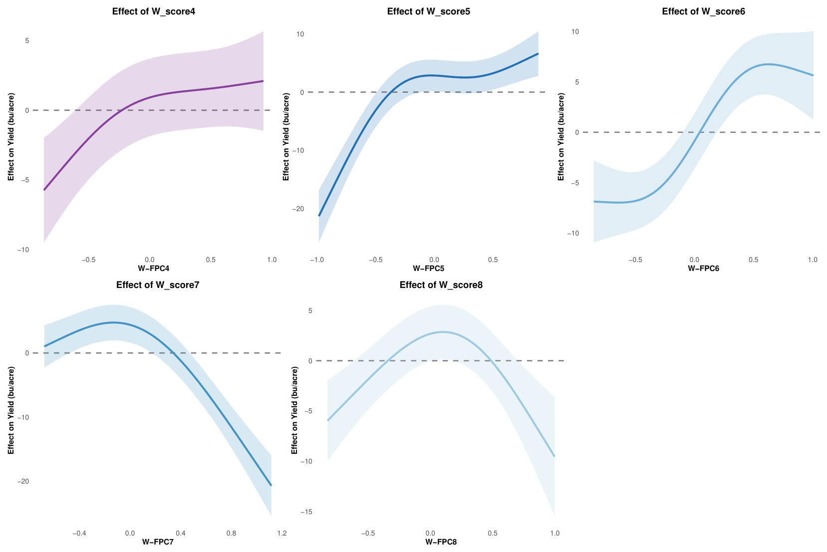
Table A1.
Methodological and conceptual comparison between the previously published SH-FAM framework and the proposed DC-FAM framework.
Figure A2.
Comparative analysis of the supplementary meteorological drivers and the physiological disaster propagation chain. (Left) The 2006 normal baseline year. (Right) The 2012 extreme flash drought year. Top panels show the daily trajectories of minimum temperature and solar radiation, while bottom panels display the continuous physiological responses of EVI and LSWI. Solid lines represent the daily observations for the respective year, and dotted or dashed lines denote the historical multi-year means. The gray shaded areas represent the historical SD envelope. In the 2012 panels, the blue and red shaded regions explicitly define the identified anomalous spring warming window and the subsequent acute flash drought stress window, respectively.
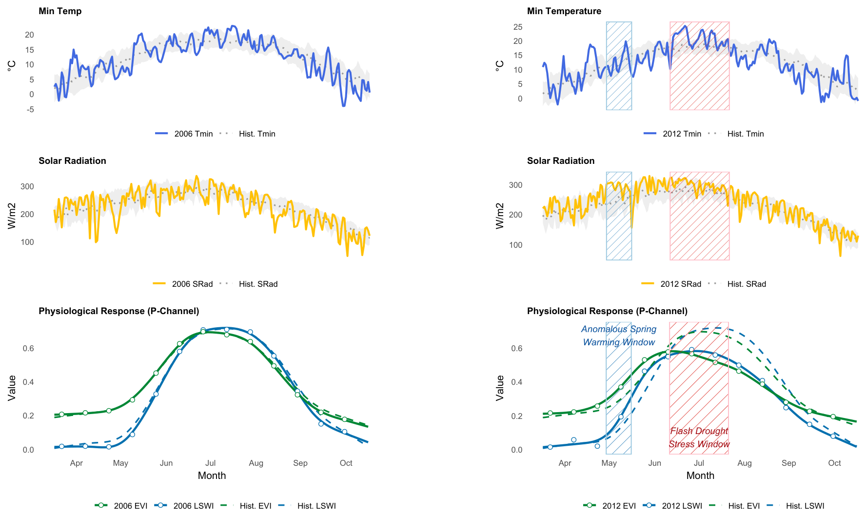
Table A2.
Paired Wilcoxon signed-rank tests comparing DC-FAM (M8) against the four principal competing models on fold-wise Weighted MSPE across 25 hold-out years.
References
- United Nations. Transforming Our World: The 2030 Agenda for Sustainable Development; UN General Assembly: New York, NY, USA, 2015; Available online: https://docs.un.org/en/A/RES/70/1 (accessed on 20 May 2026).
- Lobell, D.B.; Hammer, G.L.; McLean, G.; Messina, C.; Roberts, M.J.; Schlenker, W. The critical role of extreme heat for maize production in the United States. Nat. Clim. Change 2013, 3, 497–501. [Google Scholar] [CrossRef] [Scilit]
- Ortiz-Bobea, A.; Ault, T.R.; Carrillo, C.M.; Chambers, R.G.; Lobell, D.B. Anthropogenic climate change has slowed global agricultural productivity growth. Nat. Clim. Change 2021, 11, 306–312. [Google Scholar] [CrossRef] [Scilit]
- Otkin, J.A.; Svoboda, M.; Hunt, E.D.; Ford, T.W.; Anderson, M.C.; Hain, C.; Basara, J.B. Flash droughts: A review and assessment of the challenges dictating extreme rapid intensification of droughts. Bull. Am. Meteorol. Soc. 2018, 99, 911–919. [Google Scholar] [CrossRef] [Scilit]
- Wolf, S.; Keenan, T.F.; Fisher, J.B.; Baldocchi, D.D.; Desai, A.R.; Richardson, A.D.; Scott, R.L.; Law, B.E.; Litvak, M.E.; Brunsell, N.A.; et al. Warm spring reduced carbon cycle impact of the 2012 US summer drought. Proc. Natl. Acad. Sci. USA 2016, 113, 5880–5885. [Google Scholar] [CrossRef] [Scilit] [PubMed]
- Zhang, Y.; Keenan, T.F.; Zhou, S. Exacerbated drought impacts on global ecosystems due to structural overshoot. Nat. Ecol. Evol. 2021, 5, 1490–1498. [Google Scholar] [CrossRef] [Scilit] [PubMed]
- Holzworth, D.P.; Huth, N.I.; de Voil, P.G.; Zurcher, E.J.; Herrmann, N.I.; McLean, G.; Chenu, K.; van Oosterom, E.J.; Snow, V.; Murphy, C.; et al. APSIM – Evolution towards a new generation of agricultural systems simulation. Environ. Model. Softw. 2014, 62, 327–350. [Google Scholar] [CrossRef] [Scilit]
- Jones, J.W.; Hoogenboom, G.; Porter, C.H.; Boote, K.J.; Batchelor, W.D.; Hunt, L.A.; Wilkens, P.W.; Singh, U.; Gijsman, A.J.; Ritchie, J.T. The DSSAT cropping system model. Eur. J. Agron. 2003, 18, 235–265. [Google Scholar] [CrossRef] [Scilit]
- Schlenker, W.; Roberts, M.J. Nonlinear temperature effects indicate severe damages to US crop yields under climate change. Proc. Natl. Acad. Sci. USA 2009, 106, 15594–15598. [Google Scholar] [CrossRef] [Scilit] [PubMed]
- Shi, W.; Tao, F.; Zhang, Z. A review on statistical models for identifying climate contributions to crop yields. J. Geogr. Sci. 2013, 23, 567–576. [Google Scholar] [CrossRef] [Scilit]
- Lesk, C.; Rowhani, P.; Ramankutty, N. Influence of extreme weather disasters on global crop production. Nature 2016, 529, 84–87. [Google Scholar] [CrossRef] [Scilit] [PubMed]
- Blanc, E.; Schlenker, W. The use of panel models in assessments of climate impacts on agriculture. Rev. Environ. Econ. Policy 2017, 11, 258–279. [Google Scholar] [CrossRef] [Scilit]
- Vogel, E.; Donat, M.G.; Alexander, L.V.; Meinshausen, M.; Ray, D.K.; Karoly, D.; Meinshausen, N.; Frieler, K. The effects of climate extremes on global agricultural yields. Environ. Res. Lett. 2019, 14, 054010. [Google Scholar] [CrossRef] [Scilit]
- Ortiz-Bobea, A.; Wang, H.; Carrillo, C.M.; Ault, T.R. Unpacking the climatic drivers of US agricultural yields. Environ. Res. Lett. 2019, 14, 064003. [Google Scholar] [CrossRef] [Scilit]
- He, Y.; Qiu, B.; Cheng, F.; Chen, C.; Sun, Y.; Zhang, D.; Lin, L.; Xu, A. National Scale Maize Yield Estimation by Integrating Multiple Spectral Indexes and Temporal Aggregation. Remote Sens. 2023, 15, 414. [Google Scholar] [CrossRef] [Scilit]
- Crane-Droesch, A. A semiparametric neural network alternative to ordinary least squares for estimating climate change impacts on agriculture. Am. J. Agric. Econ. 2018, 100, 448–458. [Google Scholar] [CrossRef] [Scilit]
- Iqbal, N.; Shahzad, M.U.; Sherif, E.M.; Tariq, M.U.; Rashid, J.; Le, T.V.; Ghani, A. Analysis of Wheat-Yield Prediction Using Machine Learning Models under Climate Change Scenarios. Sustainability 2024, 16, 6976. [Google Scholar] [CrossRef] [Scilit]
- Malashin, I.; Tynchenko, V.; Gantimurov, A.; Nelyub, V.; Borodulin, A.; Tynchenko, Y. Predicting Sustainable Crop Yields: Deep Learning and Explainable AI Tools. Sustainability 2024, 16, 9437. [Google Scholar] [CrossRef] [Scilit]
- Hu, T.; Steunenberg, B.; Myers, R.J.; Ortiz-Bobea, A. Crop yield prediction via explainable AI and interpretable machine learning: Dangers of black box models for evaluating climate change impacts on crop yield. Agric. For. Meteorol. 2023, 336, 109458. [Google Scholar] [CrossRef] [Scilit]
- Wang, S.; Guan, K.; Jin, Z.; Peng, B.; Jiang, C.; Portmann, A.J.; Zhu, Q.; Wu, D.; Li, X.; Sacks, E.S.; et al. A flexible and efficient knowledge-guided machine learning data assimilation (KGML-DA) framework for agroecosystem prediction in the US Midwest. Remote Sens. Environ. 2023, 299, 113880. [Google Scholar] [CrossRef] [Scilit]
- Dong, J.; Xiao, X.; Wagle, P.; Zhang, G.; Zhou, Y.; Jin, C.; Torn, M.S.; Meyers, T.P.; Suyker, A.E.; Wang, J.; et al. Understanding the EVI and LSWI to monitor the dynamics of vegetation greenness and water content in the US Corn Belt. Agric. For. Meteorol. 2015, 214, 250–261. [Google Scholar] [CrossRef] [Scilit]
- Guan, K.; Berry, J.A.; Zhang, Y.; Joiner, J.; Guanter, L.; Badgley, G.; Lobell, D.B. Improving the monitoring of crop productivity using spaceborne solar-induced fluorescence. Glob. Change Biol. 2016, 22, 716–726. [Google Scholar] [CrossRef] [Scilit] [PubMed]
- Fahad, S.; Bajwa, A.A.; Nazir, U.; Anjum, S.A.; Farooq, A.; Zohaib, A.; Sadia, S.; Nasim, W.; Adkins, S.; Saud, S.; et al. Crop production under drought and heat stress: Plant responses and management options. Front. Plant Sci. 2017, 8, 1147. [Google Scholar] [CrossRef] [Scilit] [PubMed]
- Deines, J.M.; Kendall, A.D.; Crowley, M.A.; Kramer, J.; Hyndman, D.W. Mapping three decades of annual irrigation across the US High Plains Aquifer using Landsat and Google Earth Engine. Remote Sens. Environ. 2019, 233, 111400. [Google Scholar] [CrossRef] [Scilit]
- Basso, B.; Antle, J. Digital agriculture to design sustainable agricultural systems. Nat. Sustain. 2020, 3, 254–256. [Google Scholar] [CrossRef] [Scilit]
- Ramsay, J.O.; Silverman, B.W. Functional Data Analysis, 2nd ed.; Springer: New York, NY, USA, 2005. [Google Scholar] [CrossRef] [Scilit]
- Sartore, L.; Rosales, A.N.; Johnson, D.M.; Spiegelman, C.H. Assessing machine learning algorithms on crop yield forecasts using functional covariates derived from remotely sensed data. Comput. Electron. Agric. 2022, 194, 106704. [Google Scholar] [CrossRef] [Scilit]
- Graczyk, M.; Kurasiak-Popowska, D.; Niedziela, G. Changes in Camelina sativa Yield Based on Temperature and Precipitation Using FDA. Agriculture 2025, 15, 2051. [Google Scholar] [CrossRef] [Scilit]
- Mancini, A.; Solfanelli, F.; Coviello, L.; Martini, F.M.; Mandolesi, S.; Zanoli, R. Time Series from Sentinel-2 for Organic Durum Wheat Yield Prediction Using Functional Data Analysis and Deep Learning. Agronomy 2024, 14, 109. [Google Scholar] [CrossRef] [Scilit]
- He, X.; Luo, Y. Enhancing Agricultural Climate Resilience: A Spatially Heterogeneous Functional Framework for Corn Yield Prediction in the U.S. Midwest. Sustainability 2026, 18, 2338. [Google Scholar] [CrossRef] [Scilit]
- Reiss, P.T.; Goldsmith, J.; Shang, H.L.; Ogden, R.T. Methods for scalar-on-function regression. Int. Stat. Rev. 2017, 85, 228–251. [Google Scholar] [CrossRef] [Scilit] [PubMed]
- Park, Y.; Li, B.; Li, Y. Crop yield prediction using Bayesian spatially varying coefficient models with functional predictors. J. Am. Stat. Assoc. 2023, 118, 70–83. [Google Scholar] [CrossRef] [Scilit]
- Park, Y.; Li, B.; Li, Y. Spatially varying deep functional neural network: Application in large-scale crop yield prediction. J. R. Stat. Soc. Ser. C Appl. Stat. 2026, qlag023. [Google Scholar] [CrossRef] [Scilit]
- Malfait, N.; Ramsay, J.O. The historical functional linear model. Can. J. Stat. 2003, 31, 115–128. [Google Scholar] [CrossRef] [Scilit]
- Kim, K.; Şentürk, D.; Li, R. Recent history functional linear models for sparse longitudinal data. J. Stat. Plan. Inference 2011, 141, 1554–1566. [Google Scholar] [CrossRef] [Scilit] [PubMed]
- Chiou, J.M.; Chen, Y.T.; Yang, Y.F. Multivariate functional principal component analysis: A normalization approach. Stat. Sin. 2014, 24, 1571–1596. [Google Scholar] [CrossRef] [Scilit]
- Müller, H.G.; Yao, F. Functional additive models. J. Am. Stat. Assoc. 2008, 103, 1534–1544. [Google Scholar] [CrossRef] [Scilit]
- Jin, C.; Luo, X.; Xiao, X.; Dong, J.; Li, X.; Yang, J.; Zhao, D. The 2012 Flash Drought Threatened US Midwest Agroecosystems. Chin. Geogr. Sci. 2019, 29, 768–783. [Google Scholar] [CrossRef] [Scilit]
- Abatzoglou, J.T. Development of gridded surface meteorological data for ecological applications and modelling. Int. J. Climatol. 2013, 33, 121–131. [Google Scholar] [CrossRef] [Scilit]
- Schoener, G.; Stone, M.C. Monitoring soil moisture at the catchment scale–A novel approach combining antecedent precipitation index and radar-derived rainfall data. J. Hydrol. 2020, 589, 125155. [Google Scholar] [CrossRef] [Scilit]
- Gorelick, N.; Hancher, M.; Dixon, M.; Ilyushchenko, S.; Thau, D.; Moore, R. Google Earth Engine: Planetary-scale geospatial analysis for everyone. Remote Sens. Environ. 2017, 202, 18–27. [Google Scholar] [CrossRef] [Scilit]
- Boryan, C.; Yang, Z.; Mueller, R.; Craig, M. Monitoring US agriculture: The US Department of Agriculture, National Agricultural Statistics Service, Cropland Data Layer Program. Geocarto Int. 2011, 26, 341–358. [Google Scholar] [CrossRef] [Scilit]
- Hao, P.; Zhan, Y.; Wang, L.; Niu, Z.; Shakir, M. Feature Selection of Time Series MODIS Data for Early Crop Classification Using Random Forest: A Case Study in Kansas, USA. Remote Sens. 2015, 7, 5347–5369. [Google Scholar] [CrossRef] [Scilit]
- Zeng, L.; Wardlow, B.D.; Wang, R.; Shan, J.; Tadesse, T.; Hayes, M.J.; Li, D. A hybrid approach for detecting corn and soybean phenology with time-series MODIS data. Remote Sens. Environ. 2016, 181, 237–250. [Google Scholar] [CrossRef] [Scilit]
- Ji, Z.; Pan, Y.; Zhu, X.; Ji, J.; Adem, E.S. Crop-Mask Thresholds Optimization for Vegetation Indices in MODIS-Based Corn Yield Estimation at the United States. IEEE J. Sel. Top. Appl. Earth Obs. Remote Sens. 2026, 19, 9053–9068. [Google Scholar] [CrossRef] [Scilit]
- Brockhaus, S.; Rügamer, D.; Greven, S. Boosting functional regression models with FDboost. J. Stat. Softw. 2020, 94, 1–50. [Google Scholar] [CrossRef] [Scilit]
- Liu, X.; Lee Burras, C.; Kravchenko, Y.S.; Duran, A.; Huffman, T.; Morras, H.; Studdert, G.; Zhang, X.; Cruse, R.M.; Yuan, X. Overview of Mollisols in the world: Distribution, land use and management. Can. J. Soil Sci. 2012, 92, 383–402. [Google Scholar] [CrossRef] [Scilit]
- Valayamkunnath, P.; Barlage, M.; Chen, F.; Gochis, D.J.; Franz, K.J. Mapping of 30-m resolution tile-drained croplands using a geospatial modeling approach. Sci. Data 2020, 7, 257. [Google Scholar] [CrossRef] [Scilit] [PubMed]
- Partridge, T.F.; Winter, J.M.; Liu, L.; Kendall, A.D.; Basso, B.; Hyndman, D.W. Mid-20th century warming hole boosts US maize yields. Environ. Res. Lett. 2019, 14, 114008. [Google Scholar] [CrossRef] [Scilit]
- Bell, J.E.; Leeper, R.D.; Palecki, M.A.; Coopersmith, E.; Wilson, T.; Bilotta, R.; Embler, S. Evaluation of the 2012 Drought with a Newly Established National Soil Monitoring Network. Vadose Zone J. 2015, 14, 6. [Google Scholar] [CrossRef] [Scilit]
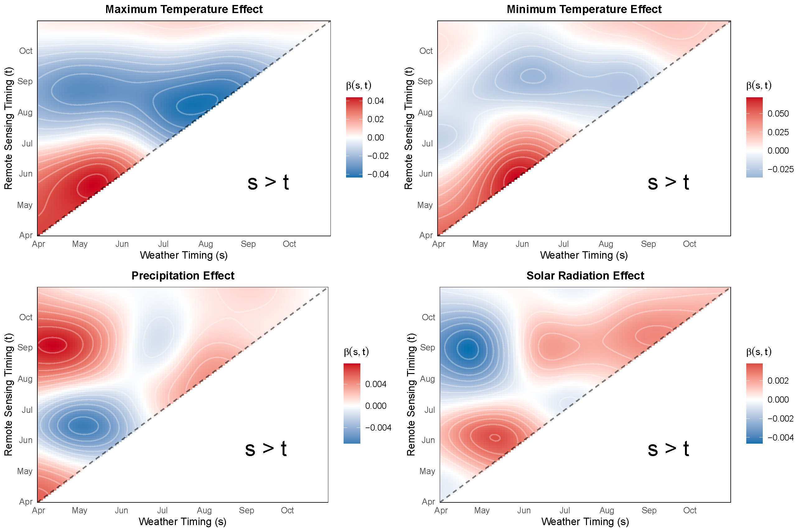
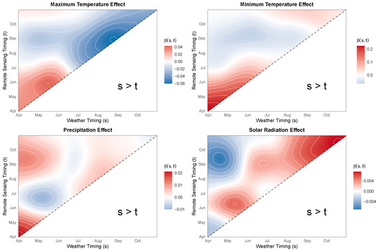
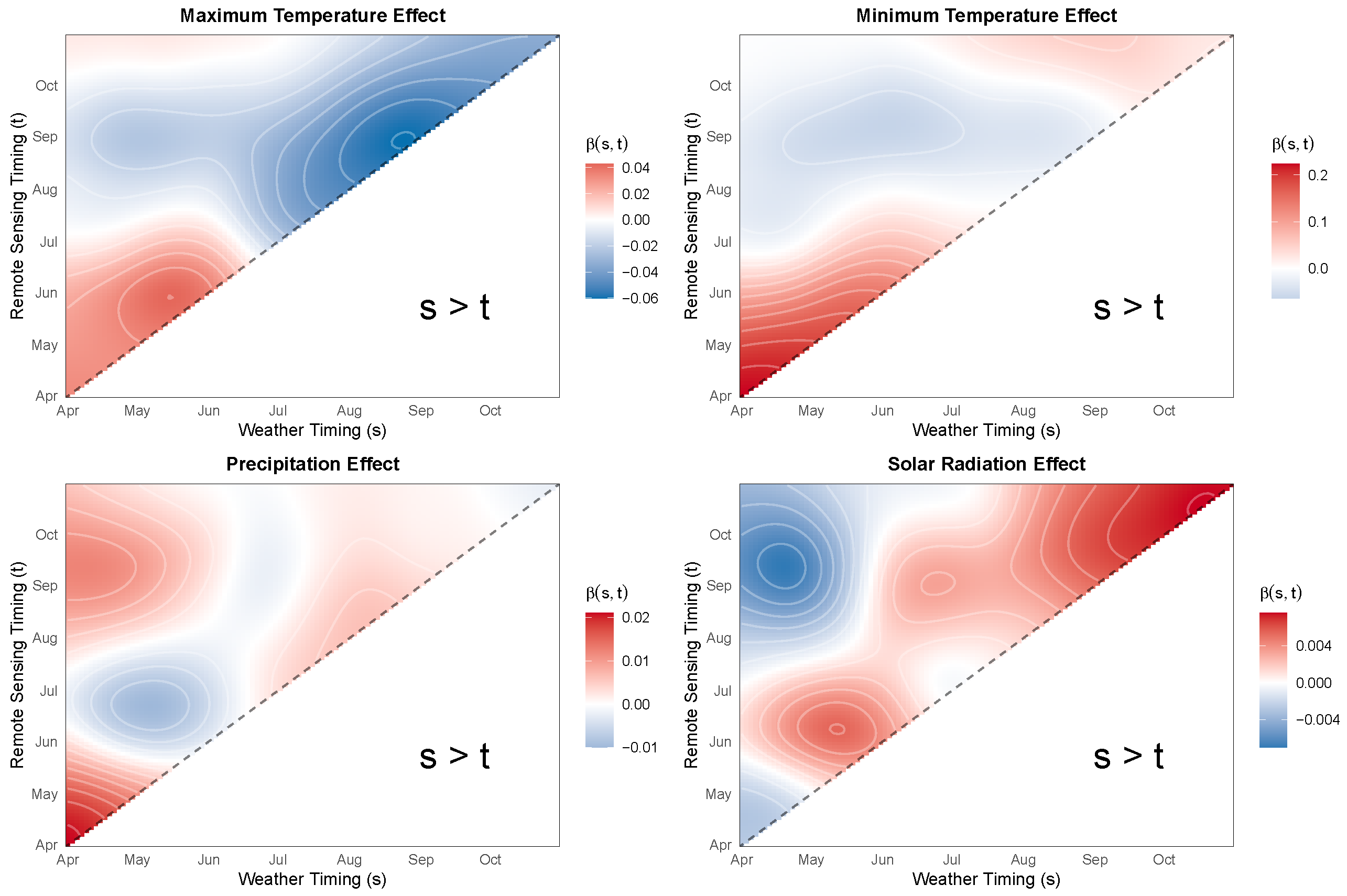
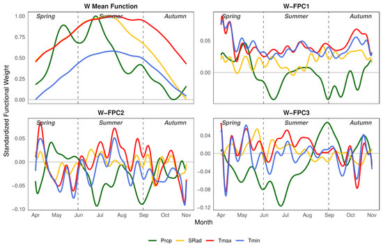
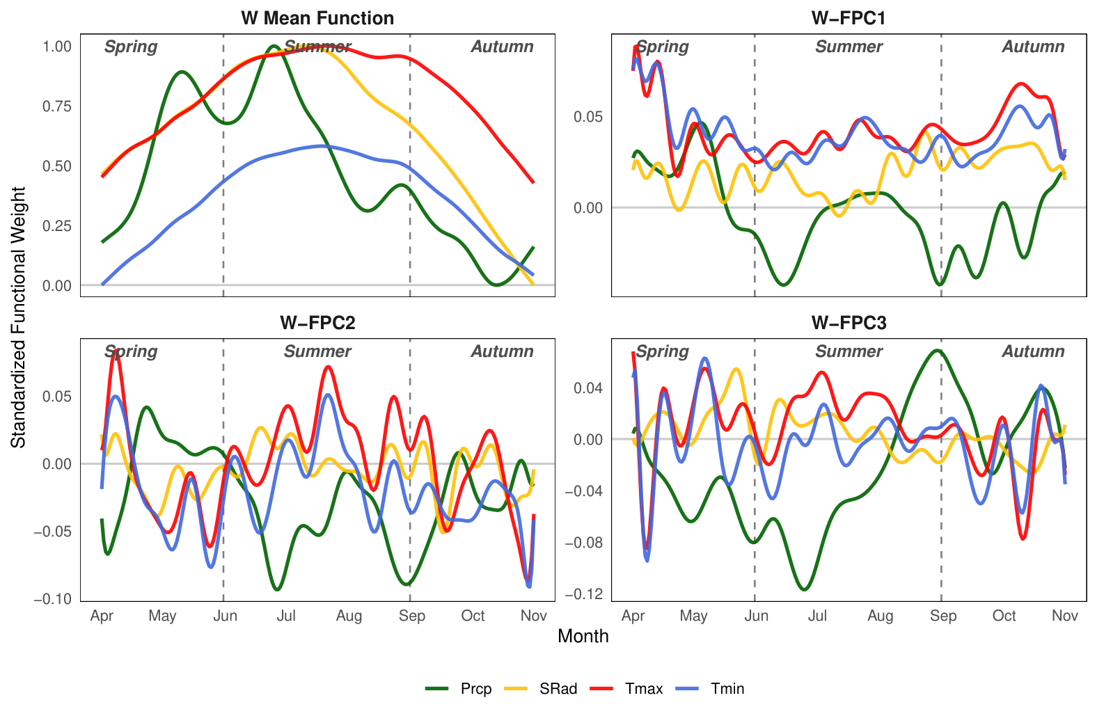
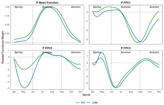
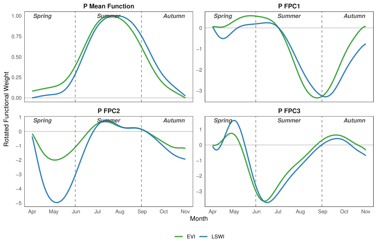
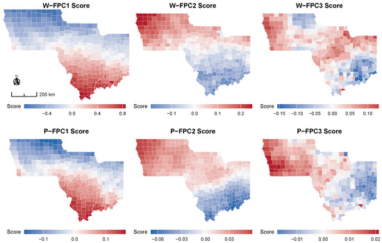
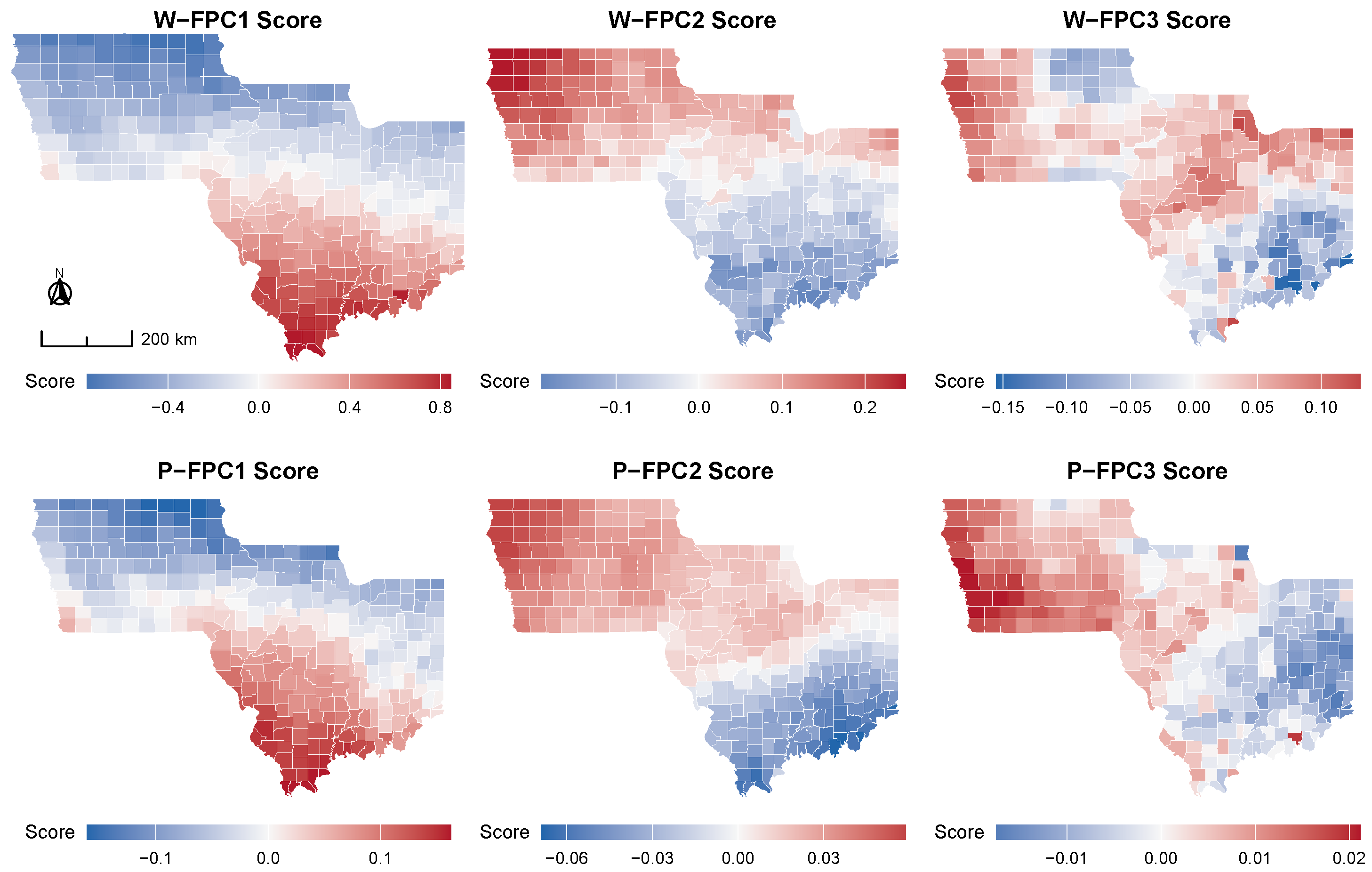
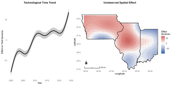
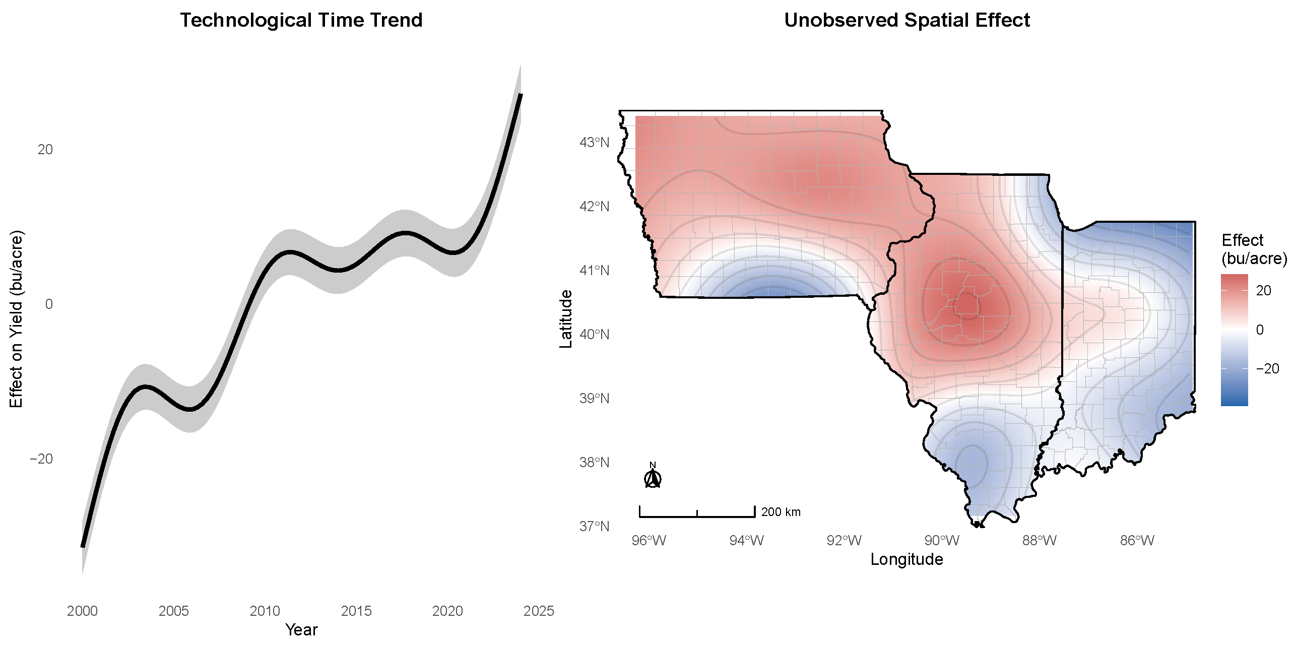
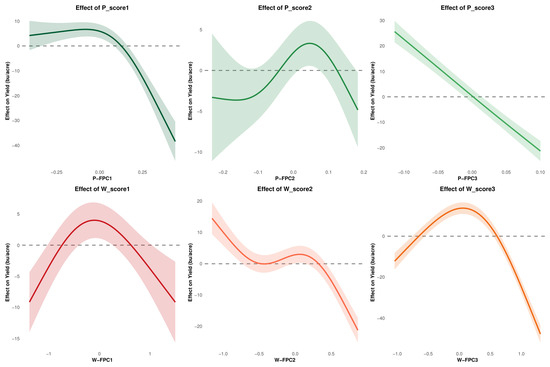
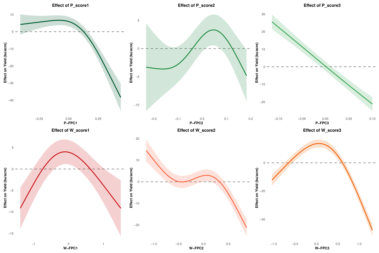
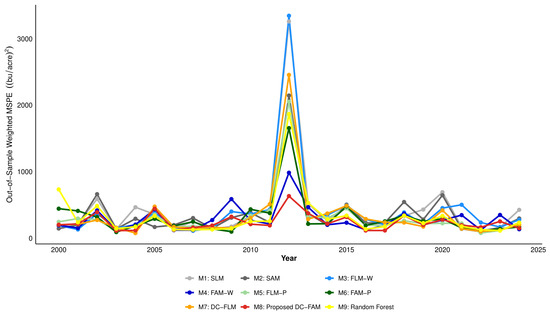
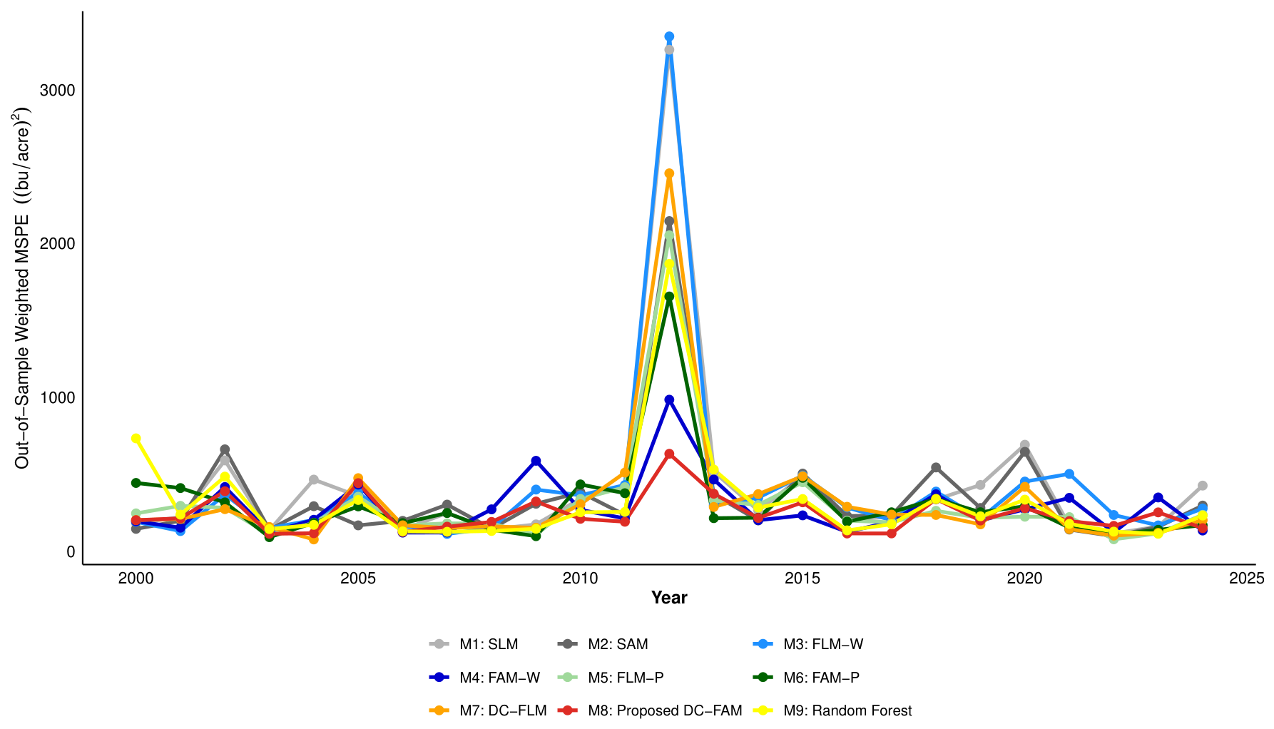
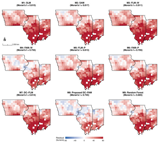
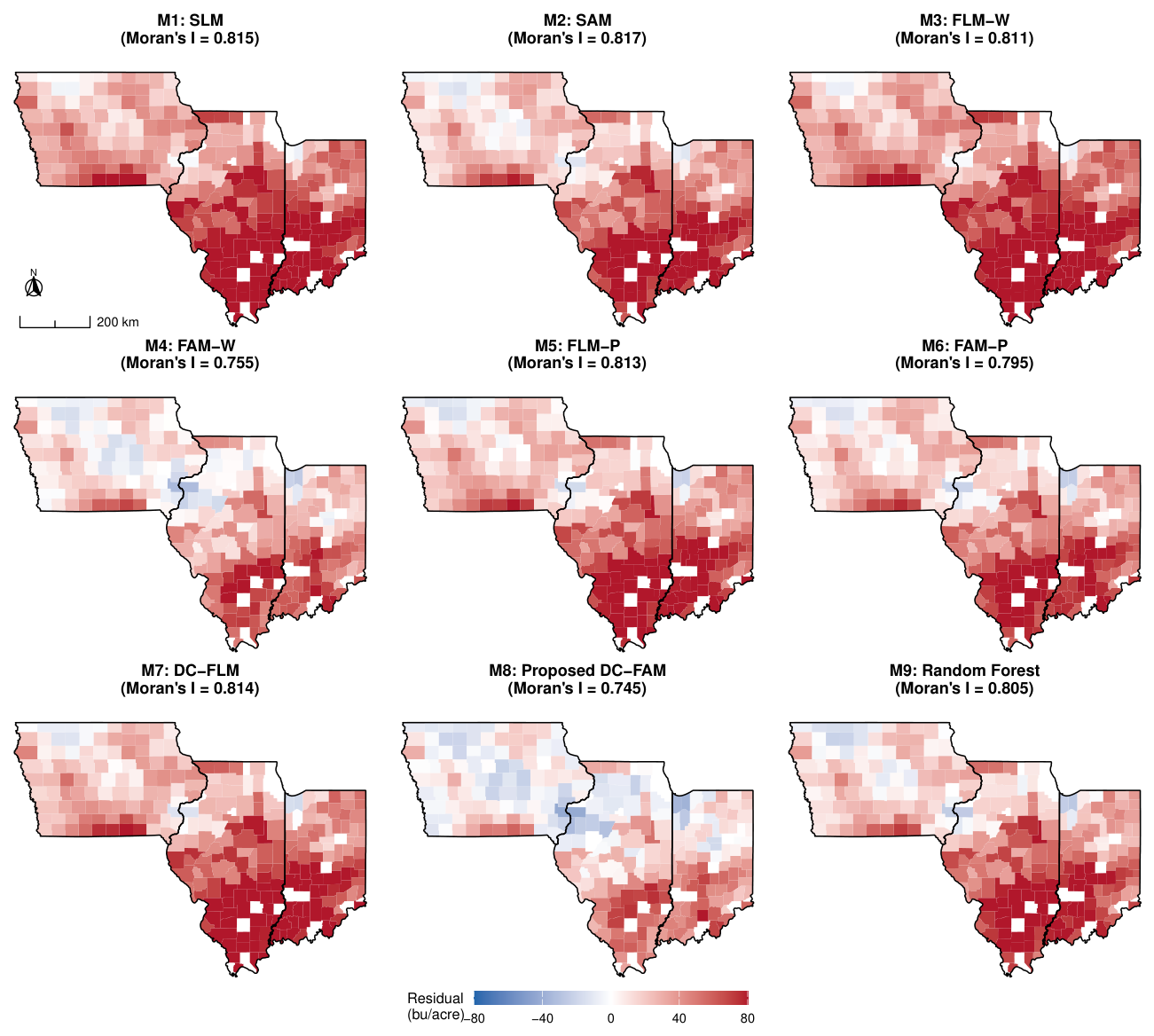
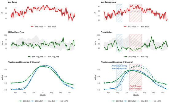
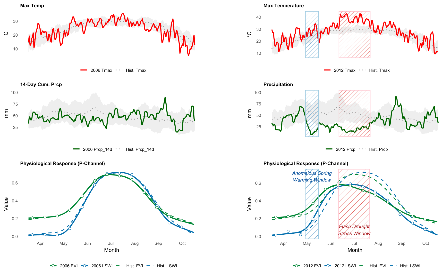

Disclaimer/Publisher’s Note: The statements, opinions and data contained in all publications are solely those of the individual author(s) and contributor(s) and not of MDPI and/or the editor(s). MDPI and/or the editor(s) disclaim responsibility for any injury to people or property resulting from any ideas, methods, instructions or products referred to in the content. |
© 2026 by the authors. Licensee MDPI, Basel, Switzerland. This article is an open access article distributed under the terms and conditions of the Creative Commons Attribution (CC BY) license.