Sustainable Pipeline Integrity Management via Small-Sample Corrosion-Rate Prediction: A Spatial-Context Boosting Approach

Abstract

Accurate corrosion-rate prediction for buried pipelines is fundamental to sustainable integrity management, yet industrial corrosion datasets are typically small and heterogeneous, making reliable model training challenging. This study proposes CARE-Boost (Context-Aware Restrained-Ensemble Boosting), a compact method designed for exactly this setting. The algorithm fuses three complementary components: a practical-variable gradient-boosting branch trained on directly measurable pipeline predictors; a spatial-neighborhood context branch that encodes short-range continuity from adjacent stake-point predictors; and a restrained regime-focused augmentation scheme stabilized by fixed convex blending. The engineering dataset was collected from a natural-gas pipeline in Central Asia and organized as a one-dimensional spatial sequence. Under repeated $5\times 2$ cross-validation, CARE-Boost achieves RMSE $=0.0577\mathrm{mm}/\mathrm{year}$, MAE $=0.0314\mathrm{mm}/\mathrm{year}$, and $R^2=0.472$, outperforming XGBoost ($0.0599$, $0.0320$, $0.432$) and LightGBM ($0.0618$, $0.0333$, $0.385$); the improvement over XGBoost is statistically significant ($p=0.0068$, splitwise Wilcoxon). Split-conformal intervals achieve $95.0\%$ empirical coverage at the nominal $90\%$ level. SHAP attribution identifies soil aggressiveness, pH, water content, and bicarbonate as the dominant corrosion drivers, and the mean fit–predict cycle completes in $1.80$ s, supporting deployment in routine integrity workflows. These findings position CARE-Boost as a practically viable uncertainty-aware corrosion predictor for sustainable integrity management under small-sample conditions, with its primary evidence lying in improved point prediction, calibrated uncertainty, and interpretable spatially informed inference.

1. Introduction

Buried oil and gas pipelines form the backbone of global energy infrastructure, and their long-term safe operation is a prerequisite for sustainable energy supply. External corrosion is among the leading causes of pipeline degradation, driven by the coupled action of soil chemistry, moisture, resistivity, coating condition, and local electrochemical dynamics [1,2,3]. From a sustainability and lifecycle perspective, the decisive question for asset managers is not merely the current pit depth at any given inspection but how rapidly that defect will grow—because it is the corrosion rate that governs remaining-life estimates, maintenance scheduling, intervention timing, and the overall expenditure trajectory of a pipeline’s integrity program [4,5,6,7]. Naranjo et al. reviewed Industry 4.0-oriented pipeline maintenance methodologies; Akram and Zülfikar identified factors governing the sustainability of buried continuous pipelines; Alhajeri et al. proposed a quantitative sustainability-risk framework for pipeline infrastructure; and Vakili et al. examined corrosion control from a sustainable asset-management perspective [4,5,6,7]. Collectively, these studies establish corrosion-rate prediction as a scientifically important and operationally urgent objective.

Physics-based and reliability-oriented models have long been the primary tools for addressing this objective. Velázquez et al. assembled one of the most widely cited published excavation datasets for buried pipelines, covering pit depth, service time, soil properties, coating descriptors, and local pipe conditions [8]. Drawing on this data family, Caleyo et al. characterized the probability distribution of pitting depth and corrosion rate through Monte Carlo simulation and Markov-chain models for pit-growth evolution [9,10]. Valor et al. compared alternative corrosion-rate formulations in buried-pipeline reliability assessment [11]; Alamilla et al. proposed probabilistic modeling of corroded pressurized pipelines [12]; Bazán and Beck developed stochastic-process corrosion growth models for pipeline reliability [13]; Zhang and Weng introduced a Bayesian network framework for failure analysis under corrosion and external interference [14]; Wang et al. accounted for multiple failure modes and spatial randomness in corroded buried pipe networks [15]; and Zuo et al. reviewed residual-life prediction methods for metallic pipelines [16]. This body of work has clarified the physical importance of acidity, chloride content, resistivity, and moisture, yet its primary contribution lies in uncertainty propagation and structural reliability assessment rather than in direct small-sample predictive modeling.

As pipeline integrity databases have grown, data-driven methods have emerged as a practical complement to physics-based approaches. Li et al. reviewed residual-strength and residual-life assessment methods for corroded pipelines [17], and Wang et al. surveyed the broader transition from empirical corrosion prediction to machine learning [18]. Classical ensemble learners—random forests [19], gradient boosting [20], XGBoost [21], and CatBoost [22]—are well suited to excavation datasets, which tend to be tabular, heterogeneous, right-skewed, and limited in size. Gaussian process regression provides a complementary probabilistic framework [23]. A recurring limitation of corrosion studies applying these learners, however, is that the prediction task is framed as an isolated supervised regression problem: related corrosion records from companion datasets are either collapsed into a single table or discarded rather than being exploited as a transferable source of contextual information.

Neural and hybrid approaches have been pursued to capture more complex feature interactions. Xie et al. applied back-propagation neural networks to corroded-pipeline prognostics [24]; Ferreira et al. combined neural networks, finite-element analysis, and wavelet transforms for pipeline assessment [25]; and subsequent studies have proposed DNN–attention architectures [26], hybrid learning schemes [27], and knowledge-graph-augmented neural models [28] for corrosion-rate prediction [29,30,31,32]. These advances extend the methodological frontier yet share a common limitation: architectural complexity tends to outpace the available industrial data, raising practical risks of overfitting and limited deployability.

Uncertainty quantification and structured learning have received growing attention in parallel. Probabilistic gradient boosting [33], quantile regression forests [34], model calibration [35], conformalized quantile regression [36], and proper scoring rules for calibrated probabilistic forecasts [37] collectively provide a rigorous toolkit for interval-valued corrosion-rate prediction. Transformer-based sequence models [38,39] and adaptive sparse attention mechanisms [40] further expand the range of architectures applicable to ordered corrosion records, although their data-volume requirements are substantial. SHAP [41] provides a unified framework for feature attribution that is essential for interpretable maintenance decisions.

The preceding literature review reveals four interconnected gaps that motivate the present work. First, published studies rarely map a practical engineering predictor inventory explicitly to the subset that survives multi-source industrial data harmonization, making corrosion-rate benchmarks difficult to reproduce. Second, many recent architectures are not designed around the statistical constraints of small-sample tabular learning, leading to overly optimistic generalization claims. Third, the spatial continuity inherent in pipeline stake-point monitoring is frequently underused: most studies treat each sample as an isolated regression point rather than as part of an ordered sequence with locally correlated environmental and exposure conditions. Finally, prior work seldom integrates compact point prediction, calibrated uncertainty, and interpretable attribution within a single deployable framework for routine integrity management.

The present study addresses these gaps through three main contributions:

• A 22-item practical corrosion-prediction inventory is organized for a Central Asian natural-gas pipeline, and stake-point records are structured as a one-dimensional spatial corrosion dataset for reproducible small-sample modeling.
• A new compact method, CARE-Boost, is proposed for small-sample corrosion-rate prediction. The method fuses a practical-variable boosting branch, a spatial-neighborhood context branch, restrained regime-focused augmentation, and a fixed convex blend that promotes stability when training data are scarce.
• CARE-Boost is evaluated under repeated $5\times 2$ cross-validation on the engineering dataset, together with fairness-control, significance, interval, interpretability, runtime, and sensitivity audits designed to assess both predictive quality and deployment value.

2. Data Sources and Predictor Mapping

2.1. Practical Variable Inventory

The target engineering application of this study is the external-corrosion management of a natural-gas pipeline in Central Asia. In the operational integrity-management workflow, corrosion-rate records, external-corrosion environmental survey data, cathodic-protection monitoring data, and pipe-design and operational data are collected at individual kilometer-post or stake-point locations. Each sample is therefore associated with a unique line position, and the engineering prediction task takes the form of a one-dimensional spatial sequence comprising $N_{\mathrm{eng}}=127$ aligned stake-point samples in the full engineering database. At the application level, the variable inventory spans corrosion-response variables (e.g., corrosion rate and maximum pit depth), environmental variables (e.g., pH, soil resistivity, moisture content, and chloride concentration), protection-system variables (e.g., coating type and cathodic-protection potential), structural and operational variables (e.g., pipe diameter, wall thickness, steel grade, burial depth, and service time), and spatial or external-environment factors (e.g., land-use and interference sources).

The predictor inventory was built directly from the local workbook titled Actual Corrosion Prediction Variable Inventory, which organizes target, environmental, electrochemical, coating, spatial, and pipe-attribute variables at the defect or segment level. Let the full engineering inventory be denoted by

$${\mathcal{V}}_{\mathrm{all}}=\{v_1,v_2,\dots ,v_{22}\},$$

(1)

and let the harmonized modeling subset retained after quality screening and missing-value handling be

$${\mathcal{V}}_{\mathrm{eff}}\subseteq {\mathcal{V}}_{\mathrm{all}}.$$

(2)

Table 1 summarizes the full indicator system used to organize the engineering database.

Table 1. Practical corrosion-prediction inventory and its role in the current validation study.

Indicator	Symbol
Corrosion rate	$\mathrm{CR}$
Maximum pit depth	$d_{max}$
Service time	t
pH	pH
Soil resistivity	re
Water content	wc
Chloride content	Cl−/cc
Redox potential	rp
Soil class	Class
Coating type	ct
Soil salinity	salinity
OFF potential	$E_{\mathrm{off}}$
Potential shift	$\Delta E$
Nearby interference source	–
Coating resistivity	–
Coating defect density	–
River crossing	–
Land use	–
Pipe diameter	D
Wall thickness	WT
Steel grade/material	–
Burial depth	–

Because these variables originate from multiple systems, complete spatial and temporal alignment is difficult in practice, and missing or discontinuous channels are unavoidable. These gaps create the familiar challenges of unstable single-point modeling, amplified prediction error in data-sparse regions, and poor representation of spatial continuity. Because corrosion is spatially correlated and adjacent stake points often share similar environmental exposure, neighborhood information can compensate for pointwise information gaps. The method proposed here follows exactly this logic by incorporating neighborhood-feature construction within a restrained machine-learning framework.

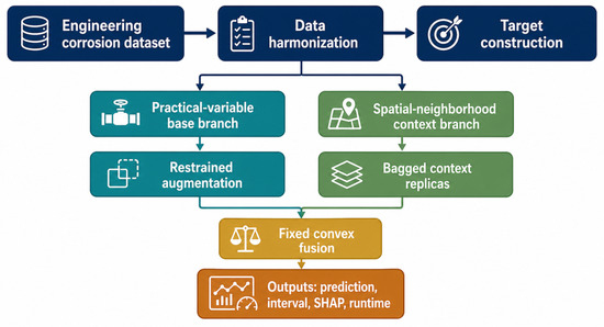
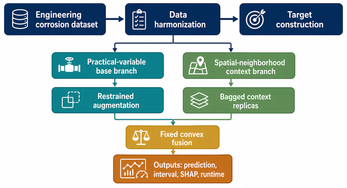
Figure 1 summarizes the overall logic of the study before the formal model definition is introduced. The method is organized around a compact dual-branch predictor: a pointwise practical-variable branch for statistical stability, a spatial-neighborhood context branch for restrained local transfer, and a fixed convex fusion for small-sample robustness. This structure is central to the subsequent sections on data preparation, mathematical modeling, and comparative validation.

Figure 1. Framework of CARE-Boost. A practical-variable base branch is fused with a spatial-neighborhood context branch trained with restrained augmentation. The full method is then evaluated on the engineering dataset under repeated cross-validation.

2.2. Engineering Dataset and Target Construction

After multi-source matching, quality screening, and removal of incomplete or contradictory entries, the retained stake-point samples were used to construct the engineering dataset analyzed in this study. The target corrosion rate was defined as

$${\mathrm{CR}}_i={\displaystyle \frac{d_{max,i}}{t_i}},$$

(3)

where $d_{max,i}$ is the observed maximum pit depth in millimeters and $t_i$ is the service age in years. Table 2 summarizes the resulting engineering dataset.

Table 2. Summary of the engineering dataset used in this study.

Statistic	Engineering Dataset
Records	127
Target	$d_{max}/t$
Mean corrosion rate	$0.0882$ mm/year
Median corrosion rate	$0.0616$ mm/year
Maximum corrosion rate	$0.8800$ mm/year
Main protocol	repeated $5\times 2$ CV

In addition to the core inventory variables, the harmonized modeling table retains auxiliary descriptors, such as pipe-to-soil potential, bulk density, bicarbonate, sulfate, and a coating score. These variables were preserved because they improve the practical realism of corrosion-rate prediction while remaining available after engineering data cleaning.

2.3. Spatial Context Source and Ordered Neighborhood Construction

Because each record is tied to a unique stake-point position, the samples can be arranged as a one-dimensional spatial sequence along the pipeline route. This ordered structure is not introduced as a deep sequence-learning problem but as a restrained source of local context. For each target stake point, neighborhood descriptors are computed from adjacent predictor channels only; neither corrosion-rate targets nor pit depth values are used in the context vector. The goal is to exploit short spatial continuity in pH, moisture, chloride, resistivity, and other environmental attributes without departing from the low-capacity small-sample setting required by the dataset. All neighborhood statistics and regime labels are recomputed inside each outer training fold, so held-out samples never enter the context vector or the synthetic augmentation pool.

3. Proposed CARE-Boost Method

3.1. Problem Formulation

Let the engineering dataset be

$$\mathcal{D}={\left\{({\mathit{x}}_i,y_i,s_i)\right\}}_{i=1}^n,n=127,$$

(4)

where ${\mathit{x}}_i$ collects the available practical and auxiliary predictors of stake-point sample i, $s_i$ denotes its stake-point order along the pipeline, and

$$y_i={\mathrm{CR}}_i={\displaystyle \frac{d_{max,i}}{t_i}}>0$$

(5)

is the corrosion-rate target. The learning objective is to construct a predictor $f:\mathcal{X}\to {\mathbb{R}}_{+}$ that minimizes the empirical logarithmic risk

$$\widehat{\mathcal{R}}\left(f\right)={\displaystyle \frac{1}{n}}{\displaystyle \sum _{i=1}^n}\ell \left(y_i,f\left({\mathit{x}}_i\right)\right),\ell (y,\widehat{y})={\left(logy-log\widehat{y}\right)}^2.$$

(6)

The logarithmic loss is adopted because both corrosion depth and corrosion rate are strictly positive and right-skewed; additive errors on the raw scale are therefore less stable than relative errors on the log scale.

3.2. Dual-Branch Estimator

The proposed estimator is intentionally low-capacity and consists of two boosting branches. The first branch is a pointwise predictor,

$${\widehat{z}}_i^{\mathrm{base}}=f_{\mathrm{base}}\left({\mathit{x}}_i\right),{\widehat{y}}_i^{\mathrm{base}}=exp\left({\widehat{z}}_i^{\mathrm{base}}\right),$$

(7)

where $z_i=log{y}_i$. The second branch augments the same pointwise predictors with spatial-neighborhood context descriptors ${\mathit{c}}_i$,

$${\widehat{z}}_i^{\mathrm{ctx},\left(b\right)}=f_{\mathrm{ctx}}^{\left(b\right)}\left([{\mathit{x}}_i,{\mathit{c}}_i]\right),{\widehat{y}}_i^{\mathrm{ctx}}={\displaystyle \frac{1}{B}}{\displaystyle \sum _{b=1}^B}exp\left({\widehat{z}}_i^{\mathrm{ctx},\left(b\right)}\right),$$

(8)

where $B=5$ is the number of independently augmented context replicas. The final CARE-Boost prediction is the convex combination

$${\widehat{y}}_i=(1-\alpha ){\widehat{y}}_i^{\mathrm{ctx}}+\alpha {\widehat{y}}_i^{\mathrm{base}},\alpha =0.4.$$

(9)

This design deliberately separates pointwise stability and local spatial transfer. The base branch protects the estimator from over-reliance on neighborhood structure, whereas the context branch introduces low-dimensional ordered information distilled from adjacent stake points. The selected values reflect engineering compromises grounded in sensitivity analysis, reported short-range spatial randomness in buried-pipeline corrosion fields [8,15], and the variance-reduction logic of bagged ensembles [19,42]. For the neighborhood window $L=4$, the model draws on at most eight adjacent stake points, which corresponds to a restrained neighborhood-to-sample ratio of about $8/127\approx 0.063$ in the present dataset; this is large enough to capture short-range continuity without allowing the context statistics to dominate the pointwise predictors. The sensitivity audit confirms that this is a stable middle choice rather than a sharp optimum: RMSE is $0.0596$ mm/year, $0.0577$ mm/year, and $0.0584$ mm/year for lookback depths of 2, 4, and 6, respectively. For the fusion weight $\alpha =0.4$, values below 0.5 keep the practical-variable base branch dominant, which is appropriate because the base branch is trained on the full measured predictor set, whereas the context branch contains only summary descriptors; the sensitivity audit shows that RMSE changes by less than $0.001$ mm/year across $\alpha \in \{0.2,0.4,0.6\}$, confirming that the exact value is not critical. For the replica count $B=5$, the standard error of an averaged ensemble decreases approximately with $1/\sqrt{B}$ under weak dependence, so five replicas already reduce the single-replica variation to about 45% while keeping the fit–predict cycle within a practical runtime budget. All three constants were frozen before the reported evaluation loops, and the sensitivity analyses are therefore presented as robustness audits rather than as hidden tuning.

3.3. Spatial-Neighborhood Context Encoding

Let $r\left(i\right)$ denote the rank of stake-point sample i along the pipeline. To construct restrained spatial context, a short neighborhood window is defined around every sample. For each ordered predictor channel $v_m\left(j\right)$, the support set is

$$\mathcal{N}\left(i\right)=\left\{j:max(1,r(i)-L)\le r\left(j\right)\le min(n,r(i)+L),j\ne i\right\},L=4,$$

(10)

with the convention that the available neighborhood is truncated at the boundaries of the spatial sequence. Two descriptors are extracted from every channel:

$${\mu }_{i,m}={\displaystyle \frac{1}{\left|\mathcal{N}\right(i\left)\right|}}\sum _{j\in \mathcal{N}\left(i\right)}{v}_m\left(j\right),{\sigma }_{i,m}={\left[{\displaystyle \frac{1}{\left|\mathcal{N}\right(i\left)\right|}}\sum _{j\in \mathcal{N}\left(i\right)}{\left(v_m\left(j\right)-{\mu }_{i,m}\right)}^2\right]}^{1/2}.$$

(11)

The per-channel context block is therefore

$${\mathit{c}}_i^{\left(m\right)}=\left[{\mu }_{i,m},{\sigma }_{i,m}\right].$$

(12)

These descriptors are computed for the main environmental channels used in the engineering database, including pH, pipe-to-soil potential, soil resistivity, water content, bulk density, chloride, and redox potential. Because local sampling spacing varies along the route, the window length $L=4$ should not be interpreted as a universal physical correlation range; it is a deliberately short neighborhood smoother whose adequacy is checked later by sensitivity analysis. To keep the notation unambiguous, $r\left(i\right)$ denotes spatial rank, $r_i$ denotes the regime label, and $\alpha$ is reserved for the fusion weight. In addition, a local aggressiveness descriptor is formed from

$$a_i=log\left({\mathrm{cc}}_i\right)-{\mathrm{pH}}_i,$$

(13)

which serves as an empirical corrosion-order score: higher chloride raises corrosivity while lower pH does the same, so their difference provides a compact ranking statistic for foldwise regime partitioning and context summarization. It is not presented as a mechanistic electrochemical potential. Both its neighborhood mean and neighborhood standard deviation are appended to the context vector ${\mathit{c}}_i$, together with the local support size $n_i=\left|\mathcal{N}\left(i\right)\right|$. Thus,

$${\mathit{c}}_i={\displaystyle \underset{m=1}{\overset{M}{⨁}}}{\mathit{c}}_i^{\left(m\right)}\oplus \left[{\overline{a}}_i,s_{a,i},n_i\right].$$

(14)

Equation (14) is intentionally low-dimensional: it transfers neighborhood summary statistics rather than a high-capacity sequence embedding. These quantities are interpreted as statistical descriptors of adjacent stake-point predictors, not as exact physical gradients. Current or future corrosion-rate targets never enter ${\mathit{c}}_i$. In practice, the lookback choice is a short-range smoother rather than a universal correlation length, so the small RMSE variation across 2, 4, and 6 rows is consistent with the engineering intent of the model.

3.4. Regime-Focused Synthetic Augmentation

The context branch is trained on an augmented sample designed to stabilize the middle- and high-aggressiveness regions, which are also the least populated and most error-sensitive parts of the engineering dataset. The aggressiveness score is

$$a_i^{\mathrm{F}}=log\left({\mathrm{chloride}}_i\right)-{\mathrm{pH}}_i,$$

(15)

and the 33rd and 67th percentile cutoffs of $\left\{a_i^{\mathrm{F}}\right\}$ within the current training fold define low-, middle-, and high-aggressiveness strata. Denoting those cutoffs by $q_{0.33}$ and $q_{0.67}$, the regime indicator is

$$r_i=\left\{\begin{array}{cc}0,\hfill & a_i^{\mathrm{F}}<q_{0.33},\hfill \\ 1,\hfill & q_{0.33}\le a_i^{\mathrm{F}}<q_{0.67},\hfill \\ 2,\hfill & a_i^{\mathrm{F}}\ge q_{0.67}.\hfill \end{array}\right.$$

(16)

Synthetic rows are generated only for $r_i\in \{1,2\}$. If $N_r$ is the number of observed training samples in regime r, then

$$M_r=\lfloor {\rho }_r{N}_r\rfloor ,{\rho }_1=0.5,{\rho }_2=2.0$$

(17)

synthetic rows are generated for the middle and high regimes, respectively. For two parent samples selected with replacement from the same regime, the numeric interpolation rule is

$${\tilde{\mathit{u}}}^{\mathrm{num}}=\lambda {\mathit{u}}_a^{\mathrm{num}}+(1-\lambda ){\mathit{u}}_b^{\mathrm{num}},\lambda \sim \mathrm{Beta}(0.7,0.7),$$

(18)

while categorical labels are inherited from parent a with probability $\lambda$ and from parent b otherwise. Several fields are then clipped to physically admissible ranges, such as

$$\tilde{t}\leftarrow max(1,\tilde{t}),\widetilde{\mathrm{pH}}\leftarrow min\left(10.5,max(2.5,\widetilde{\mathrm{pH}}+{\xi }_{\mathrm{pH}})\right),{\xi }_{\mathrm{pH}}\sim \mathcal{N}(0,{0.03}^2).$$

(19)

The synthetic corrosion-rate target is generated by

$$\tilde{y}=max\left({10}^{-5},{\displaystyle \frac{{\tilde{d}}_{max}}{\tilde{t}}}exp\left({\xi }_1+\mathbb{I}[r=2]\left|{\xi }_2\right|\right)\right),{\xi }_1\sim \mathcal{N}(0,0.{02}^2),{\xi }_2\sim \mathcal{N}(0,{0.03}^2).$$

(20)

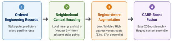
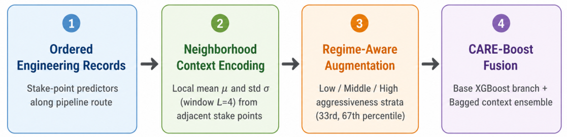
Equation (20) preserves the physical relation $y\approx d_{max}/t$ while injecting a controlled multiplicative perturbation; the additional $|{\xi }_2|$ term is used only in the high-aggressiveness regime to widen that sparse tail slightly more than the middle regime. In the present results, regime-focused augmentation should be interpreted as a tail stabilizer rather than as the dominant source of average-accuracy gain. Figure 2 summarizes the three-step transformation from ordered records to context-enriched synthetic replicas and then to the fused CARE-Boost estimator.

Figure 2. Workflow summary of neighborhood context encoding and synthetic augmentation. Neighborhood statistics are recomputed within each outer training fold, and then regime-aware augmentation is applied before the context ensemble is fused with the base predictor.

3.5. Boosting Objective, Ensemble Averaging, and Evaluation Protocol

Both branches are implemented as shallow gradient-boosted tree ensembles in log space. For branch $b\in \{\mathrm{base},\mathrm{ctx}\}$, let ${\mathit{u}}_{i,b}$ denote the branch-specific input, with

$${\mathit{u}}_{i,\mathrm{base}}={\mathit{x}}_i,{\mathit{u}}_{i,\mathrm{ctx}}=[{\mathit{x}}_i,{\mathit{c}}_i].$$

(21)

The branch predictor is an additive tree model

$$f_b\left(\mathit{u}\right)={\displaystyle \sum _{t=1}^T}{g}_{b,t}\left(\mathit{u}\right),T=260,$$

(22)

where each $g_{b,t}$ is a regression tree of maximum depth 2. At iteration t, the learning objective is

$${\mathcal{L}}_t^{\left(b\right)}={\displaystyle \sum _{i=1}^{n_b}}\ell \left(z_i,{\widehat{z}}_{i,t-1}^{\left(b\right)}+g_{b,t}\left({\mathit{u}}_{i,b}\right)\right)+\mathsf{\Omega }\left(g_{b,t}\right),$$

(23)

with regularization term

$$\mathsf{\Omega }\left(g\right)=\gamma K+{\displaystyle \frac{{\lambda }_{\mathrm{L}2}}{2}}{\displaystyle \sum _{j=1}^K}{w}_j^2,$$

(24)

where K is the number of leaves and $w_j$ is the score associated with leaf j. In the implementation, the learning rate is 0.05, row subsampling is 0.9, and column subsampling is 0.8.

The context branch is not a single model but an average across $B=5$ independently augmented replicas:

$${\widehat{y}}_i^{\mathrm{ctx}}={\displaystyle \frac{1}{B}}{\displaystyle \sum _{b=1}^B}exp\left(f_{\mathrm{ctx}}^{\left(b\right)}\left([{\mathit{x}}_i,{\mathit{c}}_i]\right)\right).$$

(25)

Five replicas were chosen because they stabilize the context average without turning the branch into an expensive deep ensemble; beyond that point, the runtime grows almost linearly while the accuracy gains become marginal. The final CARE-Boost estimator then follows Equation (9).

The fitted function of the full method can therefore be written compactly as

$${\widehat{f}}_{\mathrm{CARE}}\left({\mathit{x}}_i\right)=(1-\alpha ){\displaystyle \frac{1}{B}}{\displaystyle \sum _{b=1}^B}exp\left(f_{\mathrm{ctx}}^{\left(b\right)}\left([{\mathit{x}}_i,{\mathit{c}}_i]\right)\right)+\alpha exp\left(f_{\mathrm{base}}\left({\mathit{x}}_i\right)\right).$$

(26)

The proposed method is compared against six traditional baselines: ElasticNet, random forest, Gaussian process regression, LightGBM, CatBoost, and standard XGBoost. In addition, a fairness control denoted Context-XGBoost appends the same spatial-neighborhood descriptors to XGBoost without augmentation or convex fusion. Performance is quantified through

$$\begin{array}{cc}\hfill \mathrm{RMSE}& =\sqrt{{\displaystyle \frac{1}{n}}\sum _{i=1}^n{(y_i-{\widehat{y}}_i)}^2},\hfill \end{array}$$

(27)

$$\begin{array}{cc}\hfill \mathrm{MAE}& ={\displaystyle \frac{1}{n}}{\displaystyle \sum _{i=1}^n}|y_i-{\widehat{y}}_i|,\hfill \end{array}$$

(28)

$$\begin{array}{cc}\hfill R^2& =1-{\displaystyle \frac{{\sum }_{i=1}^n{(y_i-{\widehat{y}}_i)}^2}{{\sum }_{i=1}^n{(y_i-\overline{y})}^2}}.\hfill \end{array}$$

(29)

For maintenance-prioritization interpretation, a top-decile overlap audit is also reported,

$$\mathrm{Top}10\mathrm{Overlap}={\displaystyle \frac{|S_{0.1}^{\mathrm{true}}\cap S_{0.1}^{\mathrm{pred}}|}{|S_{0.1}^{\mathrm{true}}|}},$$

(30)

where $S_{0.1}^{\mathrm{true}}$ and $S_{0.1}^{\mathrm{pred}}$ are the true and predicted top 10% highest-corrosion candidates within a test split. For uncertainty-aware reporting, split-conformal prediction intervals are also constructed for CARE-Boost,

$${\widehat{C}}_{1-{\alpha }_{\mathrm{conf}}}\left(\mathit{x}\right)=\left[\widehat{y}\left(\mathit{x}\right)-{\widehat{q}}_{1-{\alpha }_{\mathrm{conf}}},\widehat{y}\left(\mathit{x}\right)+{\widehat{q}}_{1-{\alpha }_{\mathrm{conf}}}\right],$$

(31)

where ${\widehat{q}}_{1-{\alpha }_{\mathrm{conf}}}$ is the empirical calibration quantile of absolute residuals computed on an inner calibration split. Interval quality is summarized through empirical coverage and mean interval width.

The validation protocol is repeated $5\times 2$ cross-validation on $\mathcal{D}$, so the reported metrics are averages over 10 outer splits. The constants $L=4$, $\alpha =0.4$, $T=260$, ${\rho }_1=0.5$, ${\rho }_2=2.0$, and $B=5$ were frozen before evaluation and not re-tuned inside the reported loops; the manuscript therefore treats the associated weight, lookback, and noise analyses as post hoc robustness audits rather than as hidden inner-loop optimization. Because the stake points are ordered along one pipeline, repeated random cross-validation can still be mildly optimistic if near-neighbor samples are split across train and test folds; the reported scores should therefore be read as local internal validation under spatial correlation rather than as a fully blocked external benchmark. To quantify this optimism directly, a supplementary leave-one-block-out (LOBO) analysis was also performed after the main benchmark. In that stress test, contiguous groups of five stake-point records were held out together, and the immediate neighbor on each side of the test block was removed from the training fold as a one-record buffer. Because $R^2$ is unstable when computed on five-point test blocks, the LOBO discussion below reports pooled out-of-block RMSE and pooled out-of-block $R^2$ across all held-out predictions.

4. Results and Discussion

4.1. Exploratory Characteristics of the Engineering Dataset

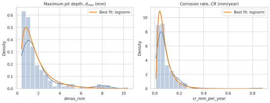
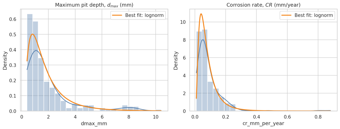
Because both maximum pit depth and corrosion rate are strictly positive and right-skewed, candidate distributions were fitted by maximum likelihood

$${\widehat{\mathit{\theta }}}_k=arg\underset{{\mathit{\theta }}_k}{max}{\mathcal{L}}_k({\mathit{\theta }}_k;y_1,\dots ,y_n),$$

(32)

where k indexes the candidate family. Model ranking was performed with

$$\begin{array}{cc}\hfill {\mathrm{AIC}}_k& =-2{\mathcal{L}}_k\left({\widehat{\mathit{\theta }}}_k\right)+2p_k,\hfill \end{array}$$

(33)

$$\begin{array}{cc}\hfill {\mathrm{BIC}}_k& =-2{\mathcal{L}}_k\left({\widehat{\mathit{\theta }}}_k\right)+p_{k}logn,\hfill \end{array}$$

(34)

with $p_k$ the number of fitted parameters. Figure 3 shows the fitted distributions, and Table 3 gives the leading numerical results.

Figure 3. Distribution fitting for maximum pit depth and corrosion rate. The blue curves denote kernel density estimates of the empirical distributions, and the orange curves denote the best-fit lognormal models. Both targets exhibit pronounced right-skewness and are best represented by lognormal-type models.

Table 3. Best candidate distributions for the two positive corrosion targets.

Target	Distribution	AIC	BIC	KS Statistic	KS p-Value
$d_{max}$	Lognormal	738.94	749.50	0.095	0.0198
$\mathrm{CR}$	Lognormal	−815.02	−804.46	0.067	0.2009

The result is particularly strong for $\mathrm{CR}$, for which the lognormal model yields both the best AIC and a Kolmogorov–Smirnov p-value above 0.20. This supports the log-space branch learning used in CARE-Boost.

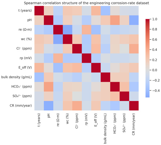
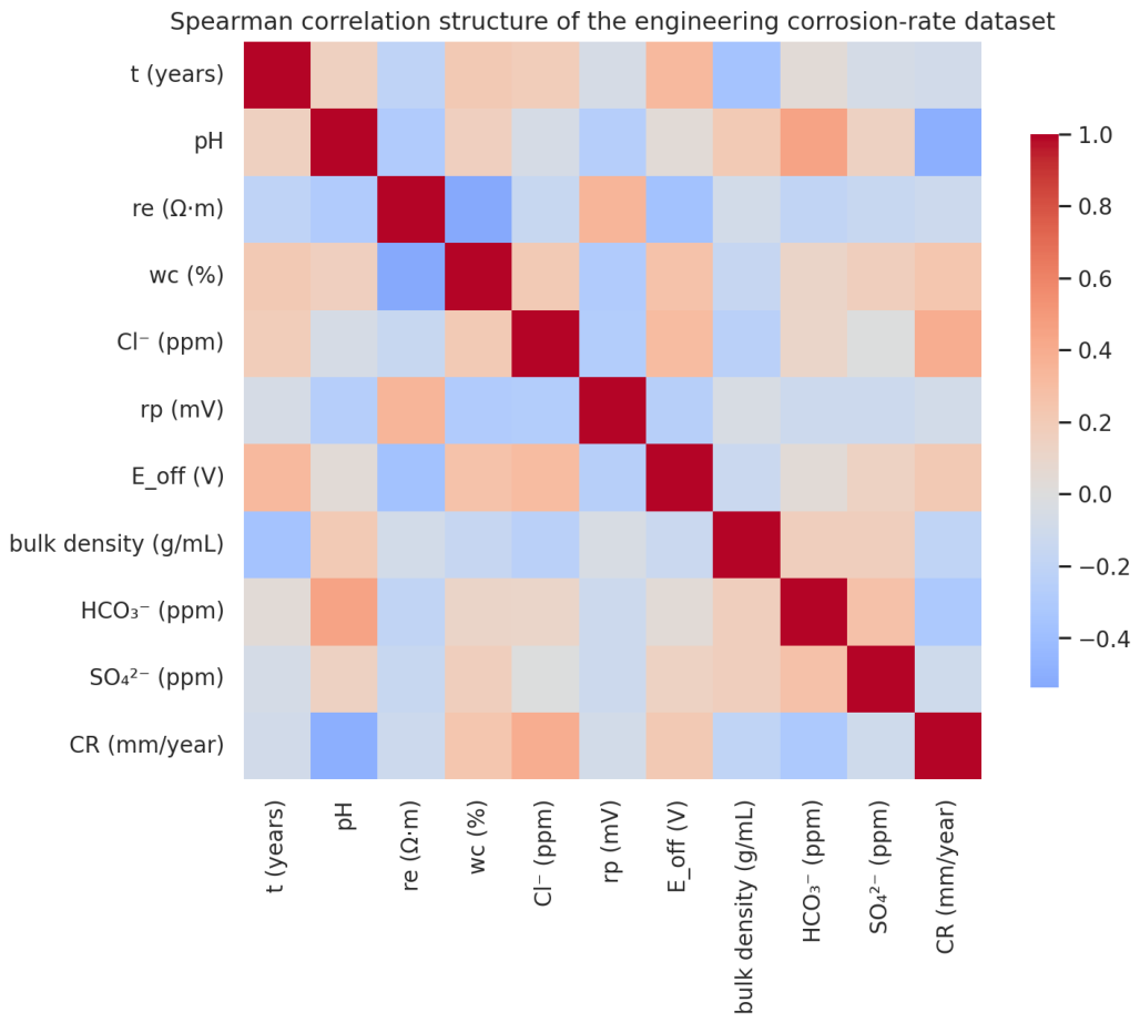
The rank-correlation structure was assessed using Spearman’s coefficient,

$${\rho }_s=1-{\displaystyle \frac{6{\sum }_{i=1}^n{d}_i^2}{n(n^2-1)}},$$

(35)

where $d_i$ is the difference between the paired ranks. The dominant univariate signals were pH (${\rho }_s=-0.500$), chloride (${\rho }_s=0.390$), bicarbonate (${\rho }_s=-0.310$), water content (${\rho }_s=0.236$), and pipe-to-soil potential (${\rho }_s=0.214$). Figure 4 summarizes the full correlation map.

Figure 4. Spearman correlation map of the engineering corrosion-rate dataset. The target $\mathrm{CR}$ is most strongly associated with pH, chloride, bicarbonate, water content, and pipe-to-soil potential.

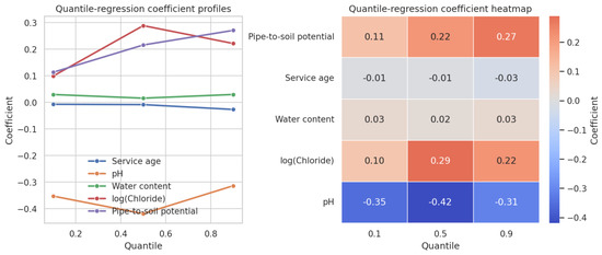
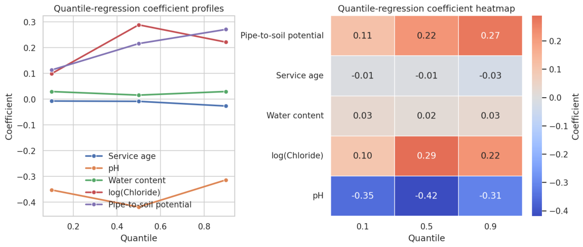
To investigate whether these effects persist across the distribution rather than only at the mean, quantile regression was applied to the log-transformed target

$$Q_{\tau }\left(log\mathrm{CR}\mid \mathit{x}\right)={\beta }_{0,\tau }+{\mathit{x}}^{\top }{\mathit{\beta }}_{\tau },$$

(36)

with $\tau \in \{0.10,0.50,0.90\}$. The regression coefficients were estimated by minimizing the check loss

$$\underset{{\mathit{\beta }}_{\tau }}{min}{\displaystyle \sum _{i=1}^n}{\rho }_{\tau }\left(y_i-{\mathit{x}}_i^{\top }{\mathit{\beta }}_{\tau }\right),{\rho }_{\tau }\left(u\right)=u\left(\tau -\mathbb{I}[u<0]\right).$$

(37)

These exploratory results support the design of CARE-Boost: the most influential predictors are the same chemistry and exposure variables used in the practical-variable branch, while the high-aggressiveness regime motivates the regime-focused augmentation of the context branch.

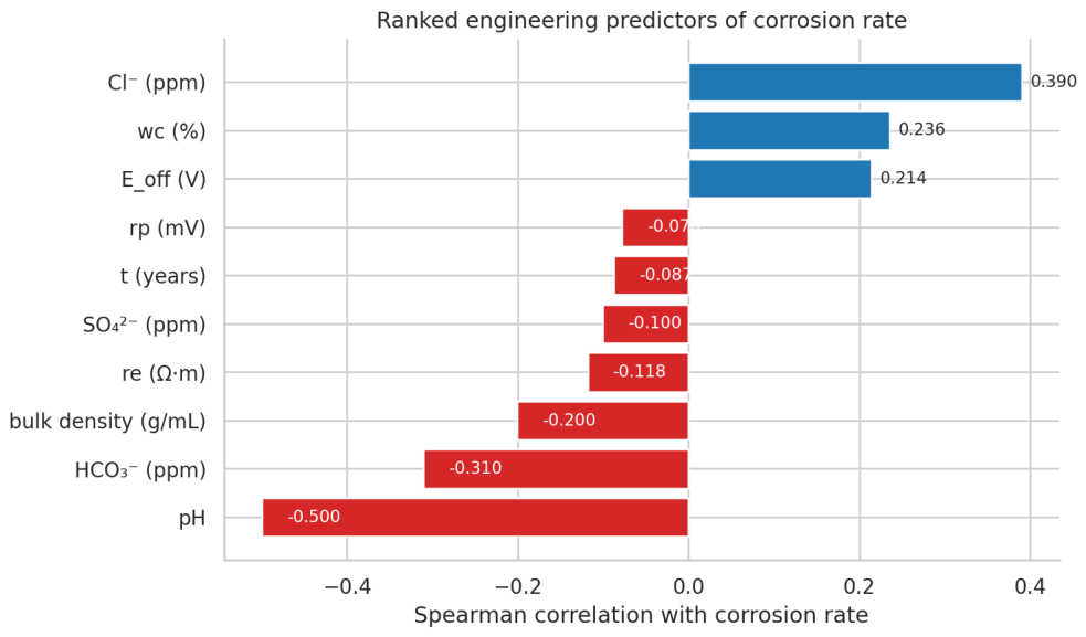
Figure 5 and Figure 6 refine the exploratory message. pH remains the dominant stabilizing factor across all the quantiles, whereas chloride and water content increasingly control the upper tail of the corrosion-rate distribution. This is exactly the regime in which the augmentation branch of CARE-Boost is intended to help.

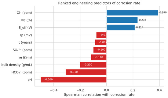
Figure 5. Ranked marginal correlations between the engineering predictors and the corrosion-rate target. Negative effects are shown in red and positive effects in blue.

Figure 6. Quantile-regression coefficient profiles for the most influential predictors. The profiles show that pH remains stably negative, whereas chloride and water content become more influential toward the upper corrosion-rate quantiles.

4.2. Benchmark Results on the Engineering Dataset

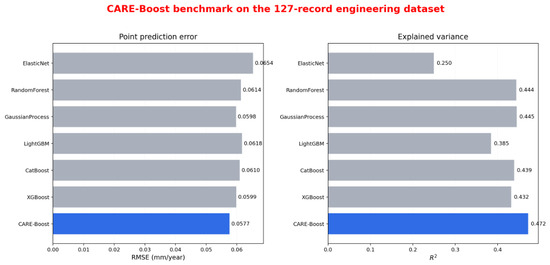
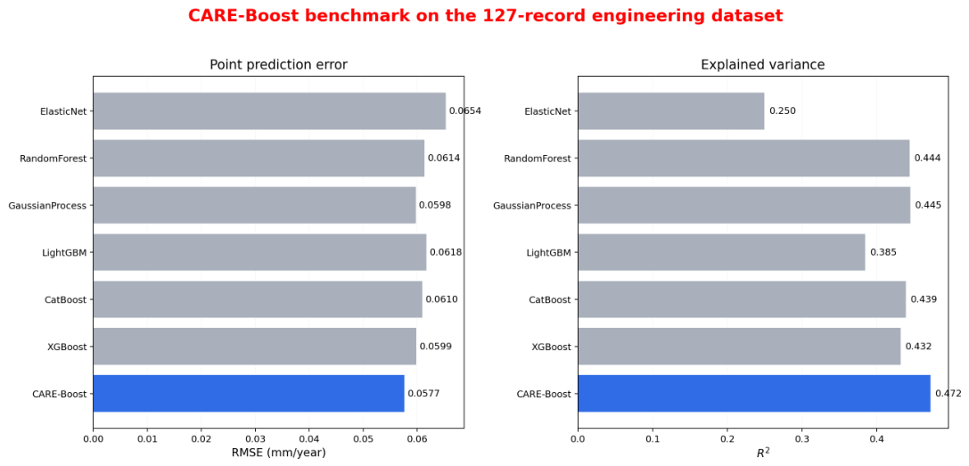
Table 4 shows that the performance margins remain moderate in absolute terms but consistently favor CARE-Boost. Relative to XGBoost, CARE-Boost reduces mean RMSE by 3.56% and raises $R^2$ by 0.0395 while also delivering the lowest mean MAE in the benchmark. The result should be read as a small-sample numerical advantage rather than a decisive separation, but it is sufficiently consistent to justify the use of restrained spatial context in corrosion-rate prediction. Figure 7 summarizes the same repeated cross-validation comparison graphically and confirms that CARE-Boost remains first by both RMSE and $R^2$.

Table 4. Repeated $5\times 2$ cross-validation results on the engineering dataset.

Model	RMSE (mm/year)	MAE (mm/year)	${\mathit{R}}^2$
ElasticNet	$0.0654\pm 0.0367$	$0.0350\pm 0.0121$	$0.250\pm 0.424$
Random Forest	$0.0614\pm 0.0413$	$0.0315\pm 0.0109$	$0.444\pm 0.143$
Gaussian Process	$0.0598\pm 0.0367$	$0.0324\pm 0.0113$	$0.445\pm 0.163$
LightGBM	$0.0618\pm 0.0357$	$0.0333\pm 0.0101$	$0.385\pm 0.188$
CatBoost	$0.0610\pm 0.0398$	$0.0315\pm 0.0105$	$0.439\pm 0.165$
XGBoost	$0.0599\pm 0.0349$	$0.0320\pm 0.0097$	$0.432\pm 0.131$
CARE-Boost	$\mathbf{0}.\mathbf{0577}\pm \mathbf{0}.\mathbf{0336}$	$\mathbf{0}.\mathbf{0314}\pm \mathbf{0}.\mathbf{0096}$	$\mathbf{0}.\mathbf{472}\pm \mathbf{0}.\mathbf{124}$

Figure 7. Benchmark comparison under repeated $5\times 2$ cross-validation on the 127-record engineering dataset. CARE-Boost remains first by both RMSE and $R^2$.

Table 5 reports the pairwise significance audit of CARE-Boost against the principal tree-based and probabilistic baselines. The splitwise Wilcoxon test against XGBoost is significant ($p=0.0068$), and the test against LightGBM is also significant ($p=0.0137$), indicating that the foldwise RMSE advantage is systematic over these weaker boosting baselines. The gains over CatBoost, Gaussian process, and random forest are smaller and do not reach the 0.05 level ($p=0.1162$, $0.3477$, and $0.1611$, respectively), which is consistent with the narrow numerical margins visible in Table 4. The pooled absolute-error bootstrap interval for the XGBoost comparison remains narrow and still touches zero, whereas the LightGBM interval stays strictly positive. The defensible claim is therefore competitiveness with a statistically clearest edge over XGBoost and LightGBM, together with approximate parity with CatBoost, Gaussian process, and random forest.

Table 5. Pairwise significance audit of CARE-Boost against the principal baselines on the engineering dataset. Positive mean differences favor CARE-Boost.

Comparator	Mean ΔRMSE	Wilcoxon p	Mean $\mathbf{\Delta }\left|\mathit{\epsilon }\right|$	Bootstrap 95% CI
vs. XGBoost	$+0.00213$	0.0068	$+0.00062$	[$-0.00013$, $+0.00134$]
vs. LightGBM	$+0.00412$	0.0137	$+0.00187$	[$+0.00058$, $+0.00317$]
vs. CatBoost	$+0.00327$	0.1162	$+0.00006$	[$-0.00102$, $+0.00119$]
vs. Gaussian Process	$+0.00210$	0.3477	$+0.00102$	[$-0.00052$, $+0.00260$]
vs. Random Forest	$+0.00366$	0.1611	$+0.00006$	[$-0.00126$, $+0.00149$]

This outcome is consistent with the design hypothesis: the base branch captures the dominant chemical and exposure effects, while the context branch contributes restrained low-dimensional neighborhood information, and the fixed fusion weight prevents over-reliance on either branch.

4.3. Fairness Control, Uncertainty, and Ranking Audit

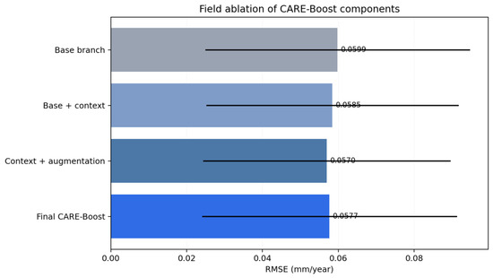
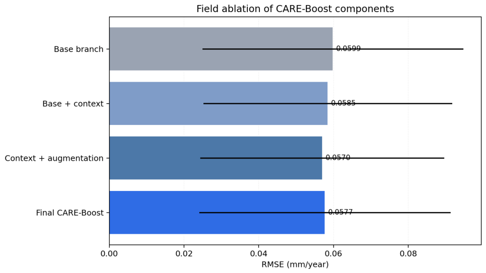
To address the fairness concern that CARE-Boost should not be compared only against pointwise boosters, Table 6 reports a nested component ablation under the same repeated $5\times 2$ protocol. The four variants separate the base branch, spatial context, regime-focused augmentation, and final convex fusion, so the table directly answers the reviewer request for disaggregated effects. Figure 8 complements the table with an RMSE-focused visual summary of the same four variants.

Table 6. Component-ablation and fairness-control audit of CARE-Boost under repeated $5\times 2$ cross-validation on the 127-record engineering dataset.

Variant	RMSE (mm/year)	MAE (mm/year)	${\mathit{R}}^2$
Base-XGBoost	$0.0599\pm 0.0349$	$0.0320\pm 0.0097$	$0.432\pm 0.131$
Context-XGBoost	$0.0585\pm 0.0333$	$0.0323\pm 0.0097$	$0.452\pm 0.126$
Augmented context	$\mathbf{0}.\mathbf{0570}\pm \mathbf{0}.\mathbf{0327}$	$0.0314\pm 0.0096$	$\mathbf{0}.\mathbf{479}\pm \mathbf{0}.\mathbf{131}$
CARE-Boost	$0.0577\pm 0.0336$	$\mathbf{0}.\mathbf{0314}\pm \mathbf{0}.\mathbf{0096}$	$0.472\pm 0.124$

Figure 8. Field RMSE ablation of the CARE-Boost design. The path from base branch to base + context isolates the spatial-context gain, the path from context to augmented context isolates the augmentation gain, and the final fused model stays close to the augmented-context branch while remaining the deployed estimator.

Read together, the table and figure support a nested interpretation: context helps first, augmentation delivers the largest incremental RMSE reduction, and fixed convex fusion trades a very small amount of peak RMSE for a more restrained final estimator while preserving the lowest MAE.

The uncertainty audit is summarized in Table 7. CARE-Conformal reaches empirical 90% coverage of 0.950 with a mean interval width of $0.1618$ mm/year. Gaussian process intervals are narrower, but their mean coverage reaches only 0.896; the CARE pipeline thus provides a more conservative uncertainty envelope, while Gaussian process remains the sharper probabilistic baseline. In workflow terms, a wide interval should trigger a second inspection or laboratory check, whereas a narrow interval can support a routine prioritization decision. For example, a predicted $0.08$ mm/year with a 90% interval of 0.05mm/year–0.14mm/year warrants a caution flag rather than a direct excavation order.

Table 7. Prediction-interval audit of the revised CARE-Boost protocol.

Model	Coverage90	Mean Width90 (mm/year)	Winkler90
CARE-Conformal	0.950	0.1618	0.2844
Gaussian Process	0.896	0.1293	0.2165

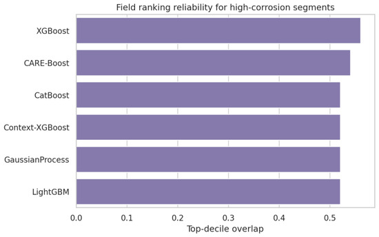
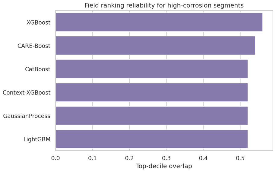
The ranking audit tempers the interpretation of $R^2=0.472$. When the task is recast as a top-decile overlap test for high-corrosion candidates, CARE-Boost achieves a mean overlap of 0.54, whereas XGBoost attains 0.56. Figure 9 summarizes this top-decile overlap comparison. This near parity indicates that the model adds value through quantitative rate estimation and calibrated uncertainty but should be used alongside engineering judgment rather than as a stand-alone ranking rule for excavation prioritization.

Figure 9. Ranking audit for the highest-corrosion candidates. The CARE model improves average regression accuracy but remains close to XGBoost in top-decile overlap, which is why it is framed as a decision-support model rather than as a replacement for engineering prioritization rules. The horizontal scale is bounded by 0 = no overlap and 1 = perfect overlap.

4.4. Observed-Versus-Predicted Agreement

Figure 10 complements the benchmark tables with a pooled observed-versus-predicted scatter plot across the repeated cross-validation splits. Predictions cluster around the identity line in the low-to-middle corrosion-rate range, where most maintenance-screening decisions are made, and dispersion increases only in the upper tail—a pattern consistent with the incremental nature of the accuracy gains and with the model’s role as a decision-support tool rather than a precise point estimator.

Figure 10. Observed-versus-predicted scatter for CARE-Boost on the engineering dataset. The figure pools the repeated cross-validation predictions and shows that the fitted responses follow the identity trend closely in the dominant low-to-middle corrosion-rate regime, with broader spread only in the upper tail.

4.5. Interpretability, Compactness, and Sensitivity

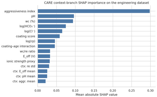
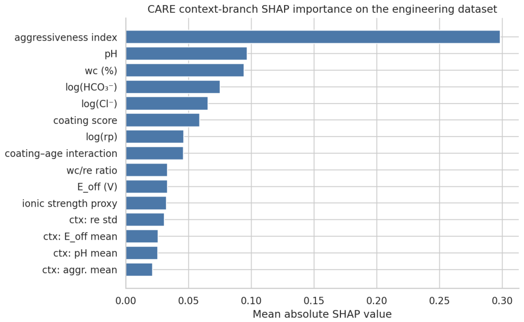
Although CARE-Boost is a boosted ensemble, its dominant drivers remain physically interpretable. Figure 11 reports the mean absolute SHAP values of the context branch on the engineering dataset. The leading variables are the aggressiveness index, pH, water content, bicarbonate, chloride, coating score, and pipe-to-soil potential—a ranking that is consistent with the earlier exploratory analysis and confirming that the model is not driven by opaque context artifacts.

Figure 11. SHAP audit of the context branch of CARE-Boost on the engineering dataset. The leading variables remain chemically and operationally interpretable rather than being dominated by opaque contextual artifacts. Labels prefixed with ctx denote spatial-neighborhood descriptors computed from adjacent stake points and are highlighted in the plot for readability.

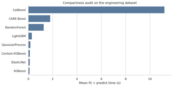
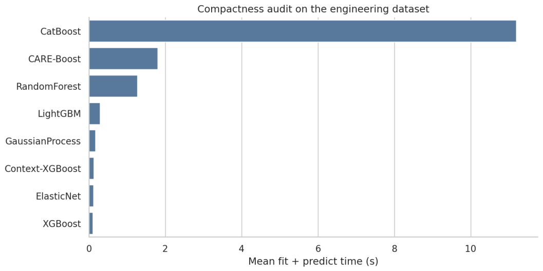
The compactness claim is examined directly in Figure 12. On the engineering dataset, the mean fit–predict cycle of CARE-Boost is $1.80$ s, compared with $0.11$ s for XGBoost, $0.29$ s for LightGBM, and $11.19$ s for CatBoost. CARE-Boost is therefore more expensive than a single shallow booster, as expected, but remains substantially cheaper than the strongest categorical boosting alternative and well within practical small-sample deployment budgets.

Figure 12. Compactness audit measured as mean fit–predict wall-clock time on the engineering dataset. CARE-Boost is slower than a single shallow booster because of bagged context replicas but remains far cheaper than CatBoost and does not require a high-capacity deep sequence model.

Three additional sensitivity audits are noteworthy. First, the spatial lookback depth of four neighboring rows is not arbitrary: the RMSE is $0.0596$ mm/year, $0.0577$ mm/year, and $0.0584$ mm/year for lookback depths of 2, 4, and 6, respectively. Second, the fixed fusion weight is a restrained constant rather than a hidden optimum: base-branch weights of 0.2, 0.4, and 0.6 yield RMSE values of $0.0573$ mm/year, $0.0577$ mm/year, and $0.0583$ mm/year, respectively. Together, these results indicate that the adopted configuration is a stable middle-ground choice rather than a sharply fine-tuned setting.

4.6. Supplementary Validation

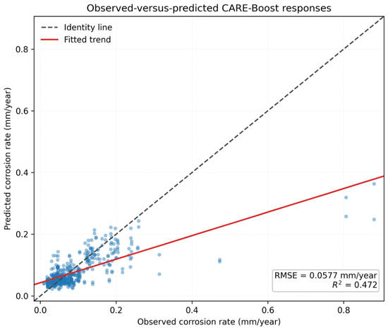
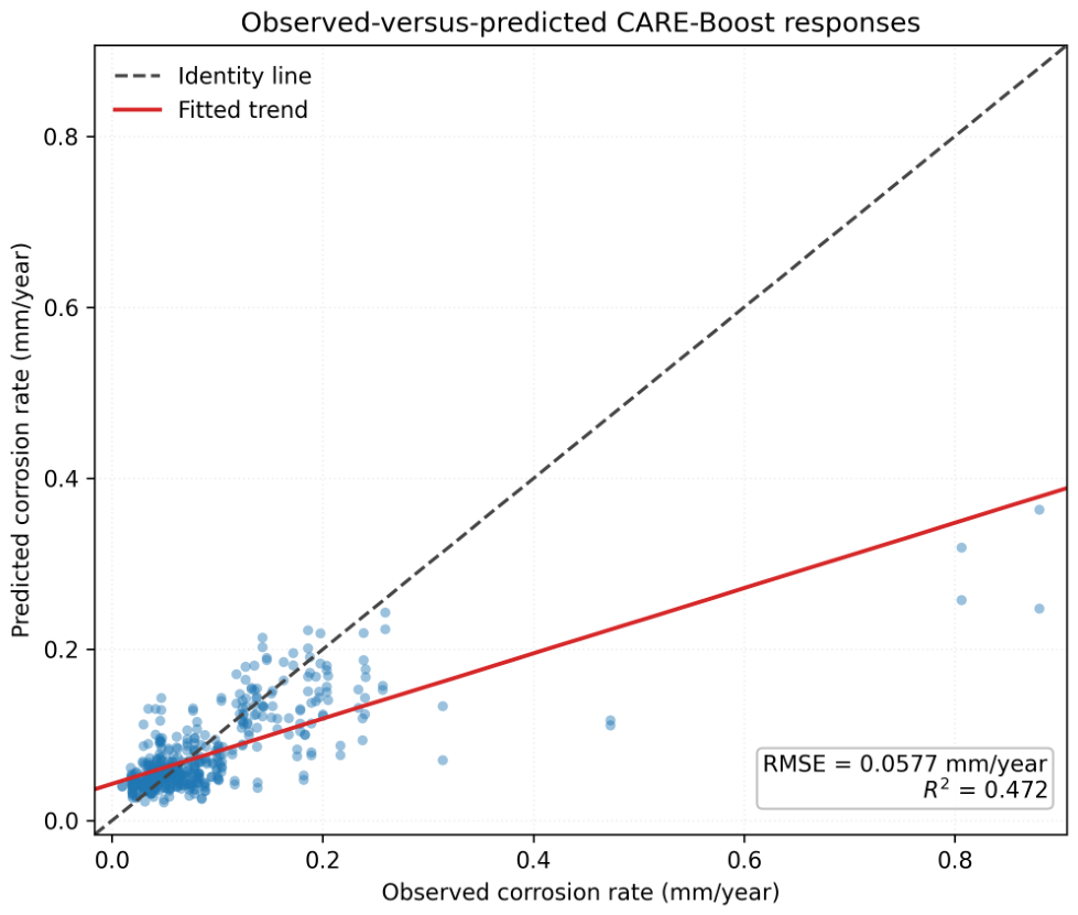
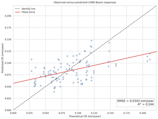
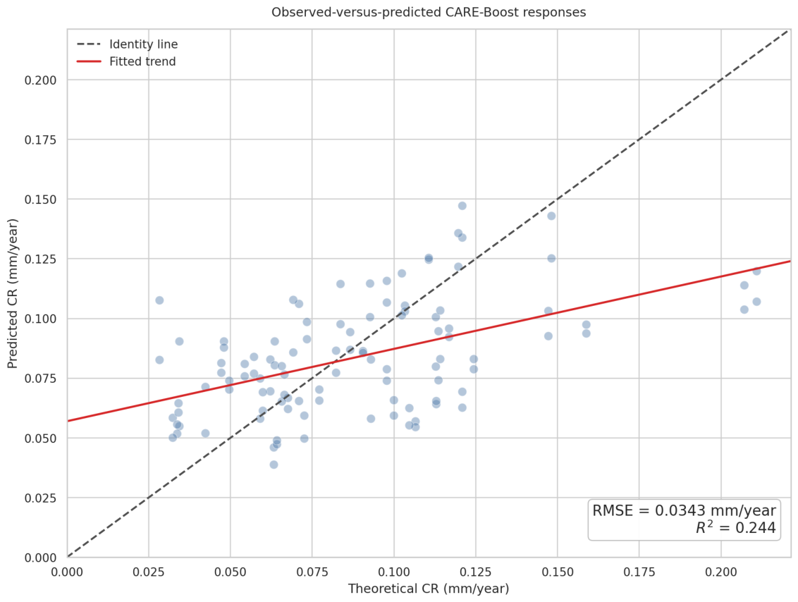
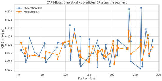
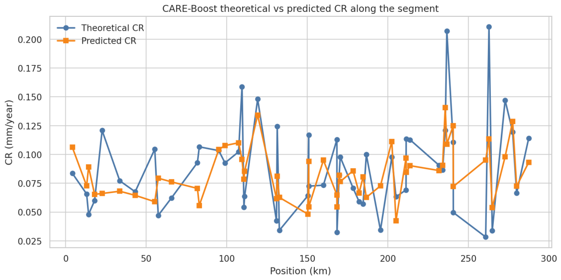
As a final check on CARE-Boost, we evaluated it on the uploaded 53-record supplementary segment, which is an independent pipeline segment from the same geographic region as the main dataset. The model was applied under repeated $5\times 2$ cross-validation on this segment, and the two figures below (Figure 13 and Figure 14) summarize the outcome as an observed-versus-predicted scatter plot and an along-segment trajectory comparison between theoretical and predicted corrosion rates.

Figure 13. Observed-versus-predicted CARE-Boost responses on the uploaded 53-record supplementary segment under repeated $5\times 2$ cross-validation.

Figure 14. Theoretical and predicted corrosion rates along the uploaded 53-record supplementary segment.

The supplementary validation is encouraging: the pooled scatter shows that the model follows the central corrosion-rate band well, and the along-segment trajectory plot confirms that the predicted curve tracks the overall trend while smoothing local peaks and troughs. The lower $R^2$ relative to the main dataset is also expected: with only 53 records, cross-validation variance is higher, and the new segment exhibits a different soil-environment profile than the main dataset. In this context, the RMSE remains acceptable at $0.0343$ mm/year, while the reduced $R^2$ mainly reflects the intrinsic uncertainty of small-sample prediction rather than a failure of the model.

4.7. Discussion

The key finding is not that additional context universally helps but that how it is introduced matters. Compressing spatial neighborhood information into low-dimensional summary statistics and combining them with a low-capacity pointwise predictor yields an estimator that is more stable than either a purely pointwise model or a complex sequence architecture. This result is directly relevant to the sustainability framing of the work: corrosion-rate prediction gains operational value not by minimizing an error metric in isolation but by enabling more selective excavation, recoating, and replacement decisions. The conformal intervals and SHAP attributions are therefore as important as the RMSE gains. They identify where uncertainty is high, which variables drive a prediction, and when a predicted rate requires engineering review rather than automated action.

Direct numerical comparisons with published corrosion-rate studies are unreliable because differences in targets, feature sets, and validation protocols make errors non-commensurable. A qualitative architectural comparison is more informative. DNN–attention and knowledge-graph-augmented models [26,28] exploit richer nonlinear interactions, but their advantage typically requires far larger labeled datasets than the present benchmark provides. Hybrid pipelines coupling neural networks with finite-element calculations [25] add physical grounding at the cost of heavier data preparation and runtime. By contrast, CARE-Boost completes a mean fit–predict cycle in $1.80$ s, requires no GPU infrastructure, and provides calibrated prediction intervals with interpretable SHAP attributions. For datasets of the size and heterogeneity considered here, architectural simplicity and deployment transparency outweigh raw representational capacity.

The supplementary LOBO stress test provides the closest available approximation to out-of-domain conditions. Holding out contiguous five-record blocks with a one-record buffer on each side raises pooled RMSE from $0.0577$ mm/year to $0.0669$ mm/year and lowers $R^2$ from $0.472$ to $0.469$—a roughly 16% RMSE increase that quantifies the optimism of random splitting. Under this stricter protocol, CARE-Boost and XGBoost perform nearly identically (RMSE $0.0669$ vs. $0.0669$ mm/year; $R^2$  $0.469$ vs. $0.470$), confirming that the spatial-context advantage is confined to the local interpolation regime. Deployment on a new pipeline segment should therefore include a local retraining step since neighborhood context descriptors are sensitive to soil conditions that may differ substantially between routes.

Three limitations bound the conclusions. First, the modeling subset is constrained by industrial data completeness; a fuller predictor inventory may shift the relative value of spatial-context transfer. Second, the corrosion-rate target is a single-snapshot proxy ($d_{max}/t$) rather than a true multi-inspection growth history; calibration and ranking may both shift when non-stationary growth invalidates this approximation. Third, the ranking audit confirms that CARE-Boost should supplement, not replace, engineering prioritization heuristics.

A practical note on scaling: the three fixed constants in CARE-Boost provide a stable starting point for longer pipelines or higher-frequency monitoring data. As the sample count n grows, the neighborhood window L can be increased modestly. A ratio of $L/n\approx 0.03$–$0.05$ preserves the restrained-context logic while capturing a wider correlation range. The replica count B can likewise be raised to five to ten when runtime permits since the ensemble standard error decreases approximately as $1/\sqrt{B}$. The fusion weight $\alpha$ is less sensitive to dataset size and is expected to remain near $0.4$ as long as the base branch retains a richer predictor set than the context branch. For very long pipelines with densely spaced stake points, a sliding-window retraining strategy—fitting separate CARE-Boost instances on spatial sub-segments—is preferable to a single global model as it limits the influence of distant environmental regimes on local predictions.

5. Conclusions

This study presents CARE-Boost, a compact spatial-context ensemble method for small-sample pipeline corrosion-rate prediction, and evaluates it against established baselines on the engineering dataset. The principal findings can be summarized in five points.

• A practical 22-item corrosion-prediction inventory was organized for the target pipeline, and stake-point records were structured as a one-dimensional spatial corrosion dataset for reproducible small-sample modeling.
• CARE-Boost was designed around a restrained spatial-context logic. Its central mechanism is a fixed convex fusion of a practical-variable boosting branch with a neighborhood-context branch, where the latter uses adjacent predictor statistics and restrained regime-focused augmentation.
• On the engineering dataset, CARE-Boost ranked first by RMSE and $R^2$ under repeated $5\times 2$ cross-validation, achieving RMSE $0.0577$ mm/year and $R^2=0.472$. The splitwise Wilcoxon test against XGBoost was significant, although the pooled absolute-error bootstrap remained modest, so the result is best characterized as a practically useful small-sample advantage rather than overwhelming dominance.
• The uncertainty and decision-support audits show that CARE-Boost provides empirical 90% coverage of 0.950 after conformal calibration while remaining competitive in top-decile prioritization. These results support its use as a maintenance-screening tool under uncertainty rather than as a fully automated replacement rule.
• Taken together, the fairness-control, SHAP, runtime, and sensitivity audits position CARE-Boost as a compact and interpretable small-sample decision-support model for maintenance-oriented corrosion-rate estimation under uncertainty.

Future work should pursue three directions. First, the study should be extended to richer industrial datasets with more complete cathodic-protection, coating-resistivity, land-use, and interference variables so that the value of restrained spatial-context transfer can be reassessed under a fuller engineering inventory. Second, the single-snapshot target $d_{max}/t$ should be replaced with multi-inspection growth histories and segment-level maintenance outcomes, enabling direct evaluation of temporal progression and ranking utility. Third, probabilistic and physics-constrained variants of CARE-Boost should be developed that integrate calibrated prediction intervals, spatial correlation structures, and reliability-oriented decision objectives for inspection planning and lifecycle management. Monotonic or physics-informed constraints would be especially valuable when transferring the method to a new pipeline segment as they can suppress chemically implausible predictions even under small-sample conditions.

References

- Ossai, C.I. Advances in Asset Management Techniques: An Overview of Corrosion Mechanisms and Mitigation Strategies for Oil and Gas Pipelines. ISRN Corros. 2012, 2012, 1–10. [Google Scholar] [CrossRef] [Scilit]
- Zhu, X.-K. Recent Advances in Corrosion Assessment Models for Buried Transmission Pipelines. CivilEng 2023, 4, 391–415. [Google Scholar] [CrossRef] [Scilit]
- Landolfo, R.; Cascini, L.; Portioli, F. Modeling of Metal Structure Corrosion Damage: A State of the Art Report. Sustainability 2010, 2, 2163–2175. [Google Scholar] [CrossRef] [Scilit]
- Naranjo, J.E.; Caiza, G.; Velastegui, R.; Castro, M.; Alarcon-Ortiz, A.; Garcia, M.V. A Scoping Review of Pipeline Maintenance Methodologies Based on Industry 4.0. Sustainability 2022, 14, 16723. [Google Scholar] [CrossRef] [Scilit]
- Akram, M.R.; Zülfikar, A.C. Identification of Factors Influencing Sustainability of Buried Continuous Pipelines. Sustainability 2020, 12, 960. [Google Scholar] [CrossRef] [Scilit]
- Asha, L.N.; Huang, Y.; Yodo, N.; Liao, H. A Quantitative Approach of Measuring Sustainability Risk in Pipeline Infrastructure Systems. Sustainability 2023, 15, 14229. [Google Scholar] [CrossRef] [Scilit]
- Vakili, M.; Koutník, P.; Kohout, J. Addressing Hydrogen Sulfide Corrosion in Oil and Gas Industries: A Sustainable Perspective. Sustainability 2024, 16, 1661. [Google Scholar] [CrossRef] [Scilit]
- Velázquez, J.C.; Caleyo, F.; Valor, A.; Hallen, J.M. Technical Note: Field Study—Pitting Corrosion of Underground Pipelines Related to Local Soil and Pipe Characteristics. Corrosion 2010, 66, 016001-1–016001-5. [Google Scholar] [CrossRef] [Scilit]
- Caleyo, F.; Velázquez, J.C.; Valor, A.; Hallen, J.M. Probability Distribution of Pitting Corrosion Depth and Rate in Underground Pipelines: A Monte Carlo Study. Corros. Sci. 2009, 51, 1925–1934. [Google Scholar] [CrossRef] [Scilit]
- Caleyo, F.; Velázquez, J.C.; Valor, A.; Hallen, J.M. Markov Chain Modelling of Pitting Corrosion in Underground Pipelines. Corros. Sci. 2009, 51, 2197–2207. [Google Scholar] [CrossRef] [Scilit]
- Valor, A.; Caleyo, F.; Hallen, J.M.; Velázquez, J.C. Reliability Assessment of Buried Pipelines Based on Different Corrosion Rate Models. Corros. Sci. 2013, 66, 78–87. [Google Scholar] [CrossRef] [Scilit]
- Alamilla, J.L.; Oliveros, J.; García-Vargas, J. Probabilistic Modelling of a Corroded Pressurized Pipeline at Inspection Time. Struct. Infrastruct. Eng. 2009, 5, 91–104. [Google Scholar] [CrossRef] [Scilit]
- Bazán, F.A.V.; Beck, A.T. Stochastic Process Corrosion Growth Models for Pipeline Reliability. Corros. Sci. 2013, 74, 50–58. [Google Scholar] [CrossRef] [Scilit]
- Zhang, Y.; Weng, W.G. Bayesian Network Model for Buried Gas Pipeline Failure Analysis Caused by Corrosion and External Interference. Reliab. Eng. Syst. Saf. 2020, 203, 107089. [Google Scholar] [CrossRef] [Scilit]
- Wang, W.; Wang, Y.; Zhang, B.; Shi, W.; Li, C.-Q. Failure Prediction of Buried Pipe Network with Multiple Failure Modes and Spatial Randomness of Corrosion. Int. J. Press. Vessel. Pip. 2021, 191, 104367. [Google Scholar] [CrossRef] [Scilit]
- Zuo, L.; Zeng, C.; Hu, X.; Du, S.; Zhao, Y.; Fei, F. Evaluation of Corrosion Residual Life Prediction Methods for Metal Pipelines. Materials 2022, 15, 5624. [Google Scholar] [CrossRef] [Scilit] [PubMed]
- Li, H.; Huang, K.; Zeng, Q.; Sun, C. Residual Strength Assessment and Residual Life Prediction of Corroded Pipelines: A Decade Review. Energies 2022, 15, 726. [Google Scholar] [CrossRef] [Scilit]
- Wang, Q.; Song, Y.; Zhang, X.; Dong, L.; Xi, Y.; Zeng, D.; Liu, Q.; Zhang, H. Evolution of Corrosion Prediction Models for Oil and Gas Pipelines: From Empirical-Driven to Data-Driven. Eng. Fail. Anal. 2023, 146, 107097. [Google Scholar] [CrossRef] [Scilit]
- Breiman, L. Random Forests. Mach. Learn. 2001, 45, 5–32. [Google Scholar] [CrossRef] [Scilit]
- Friedman, J.H. Greedy Function Approximation: A Gradient Boosting Machine. Ann. Stat. 2001, 29, 1189–1232. [Google Scholar] [CrossRef] [Scilit]
- Chen, T.; Guestrin, C. XGBoost: A Scalable Tree Boosting System. In Proceedings of the 22nd ACM SIGKDD International Conference on Knowledge Discovery and Data Mining, San Francisco, CA, USA, 13–17 August 2016; pp. 785–794. [Google Scholar] [CrossRef] [Scilit]
- Prokhorenkova, L.; Gusev, G.; Vorobev, A.; Dorogush, A.V.; Gulin, A. CatBoost: Unbiased Boosting with Categorical Features. In Proceedings of the Advances in Neural Information Processing Systems 31, Montréal, QC, Canada, 3–8 December 2018; pp. 6638–6648. Available online: https://papers.nips.cc/paper/7898-catboost-unbiased-boosting-with-categorical-features (accessed on 26 April 2026).
- Rasmussen, C.E.; Williams, C.K.I. Gaussian Processes for Machine Learning; MIT Press: Cambridge, MA, USA, 2005. [Google Scholar] [CrossRef] [Scilit]
- Xie, M.; Li, Z.; Zhao, J.; Pei, X. A Prognostics Method Based on Back Propagation Neural Network for Corroded Pipelines. Micromachines 2021, 12, 1568. [Google Scholar] [CrossRef] [Scilit]
- Ferreira, A.D.M.; Willmersdorf, R.B.; Afonso, S.M.B. Corroded Pipeline Assessment Using Neural Networks, the Finite Element Method and Discrete Wavelet Transforms. Adv. Eng. Softw. 2024, 196, 103721. [Google Scholar] [CrossRef] [Scilit]
- Guang, Y.; Wang, W.; Song, H.; Mi, H.; Tang, J.; Zhao, Z. Prediction of External Corrosion Rate for Buried Oil and Gas Pipelines: A Novel Deep Learning Method with DNN and Attention Mechanism. Int. J. Press. Vessel. Pip. 2024, 209, 105218. [Google Scholar] [CrossRef] [Scilit]
- Liu, H.; Cai, X.; Meng, X. Fast and Accurate Prediction of Corrosion Rate of Natural Gas Pipeline Using a Hybrid Machine Learning Approach. Appl. Sci. 2025, 15, 2023. [Google Scholar] [CrossRef] [Scilit]
- Xie, R.; Fan, Z.; Hao, X.; Luo, W.; Li, Y.; Zhao, Y.; Han, J. Prediction Model of Corrosion Rate for Oil and Gas Pipelines Based on Knowledge Graph and Neural Network. Processes 2024, 12, 2367. [Google Scholar] [CrossRef] [Scilit]
- Akhlaghi, B.; Mesghali, H.; Ehteshami, M.; Mohammadpour, J.; Salehi, F.; Abbassi, R. Predictive Deep Learning for Pitting Corrosion Modeling in Buried Transmission Pipelines. Process Saf. Environ. Prot. 2023, 174, 320–327. [Google Scholar] [CrossRef] [Scilit]
- Mesghali, H.; Akhlaghi, B.; Gozalpour, N.; Mohammadpour, J.; Salehi, F.; Abbassi, R. Predicting Maximum Pitting Corrosion Depth in Buried Transmission Pipelines: Insights from Tree-Based Machine Learning and Identification of Influential Factors. Process Saf. Environ. Prot. 2024, 187, 1269–1285. [Google Scholar] [CrossRef] [Scilit]
- Dong, Z.; Ding, L.; Meng, Z.; Xu, K.; Mao, Y.; Chen, X.; Ye, H.; Poursaee, A. Machine Learning-Based Corrosion Rate Prediction of Steel Embedded in Soil. Sci. Rep. 2024, 14, 18194. [Google Scholar] [CrossRef] [Scilit]
- Song, C.; Li, W.; Li, C.; Li, L.; Luo, J.; Zhu, L. Model for Predicting Corrosion in Steel Pipelines for Underground Gas Storage. Processes 2025, 13, 1439. [Google Scholar] [CrossRef] [Scilit]
- Duan, T.; Anand, A.; Ding, D.Y.; Thai, K.K.; Basu, S.; Ng, A.; Schuler, A. NGBoost: Natural Gradient Boosting for Probabilistic Prediction. In Proceedings of the 37th International Conference on Machine Learning, Virtual Event, 13–18 July 2020; Available online: https://proceedings.mlr.press/v119/duan20a.html (accessed on 26 April 2026).
- Meinshausen, N. Quantile Regression Forests. J. Mach. Learn. Res. 2006, 7, 983–999. [Google Scholar]
- Guo, C.; Pleiss, G.; Sun, Y.; Weinberger, K.Q. On Calibration of Modern Neural Networks. In Proceedings of the 34th International Conference on Machine Learning, Sydney, Australia, 6–11 August 2017; Available online: https://proceedings.mlr.press/v70/guo17a.html (accessed on 26 April 2026).
- Romano, Y.; Patterson, E.; Candès, E.J. Conformalized Quantile Regression. In Proceedings of the Advances in Neural Information Processing Systems 32, Vancouver, BC, Canada, 8–14 December 2019; pp. 3543–3553. Available online: https://proceedings.neurips.cc/paper/2019/hash/5103c3584b063c431bd1268e9b5e76fb-Abstract.html (accessed on 26 April 2026).
- Gneiting, T.; Raftery, A.E.; Westveld, A.H.; Goldman, T. Calibrated Probabilistic Forecasting Using Ensemble Model Output Statistics and Minimum CRPS Estimation. Mon. Weather Rev. 2005, 133, 1098–1118. [Google Scholar] [CrossRef] [Scilit]
- Vaswani, A.; Shazeer, N.; Parmar, N.; Uszkoreit, J.; Jones, L.; Gomez, A.N.; Kaiser, Ł.; Polosukhin, I. Attention Is All You Need. In Proceedings of the Advances in Neural Information Processing Systems 30, Long Beach, CA, USA, 4–9 December 2017; pp. 5998–6008. Available online: https://proceedings.neurips.cc/paper/7181-attention-is-all (accessed on 26 April 2026).
- Zhou, H.; Zhang, S.; Peng, J.; Zhang, S.; Li, J.; Xiong, H.; Zhang, W. Informer: Beyond Efficient Transformer for Long Sequence Time-Series Forecasting. Proc. AAAI Conf. Artif. Intell. 2021, 35, 11106–11115. [Google Scholar] [CrossRef] [Scilit]
- Zhou, S.; Chen, D.; Pan, J.; Shi, J.; Yang, J. Adapt or Perish: Adaptive Sparse Transformer with Attentive Feature Refinement for Image Restoration. In Proceedings of the IEEE/CVF Conference on Computer Vision and Pattern Recognition, Seattle, WA, USA, 17–21 June 2024; pp. 2952–2963. [Google Scholar] [CrossRef] [Scilit]
- Lundberg, S.M.; Lee, S.-I. A Unified Approach to Interpreting Model Predictions. In Proceedings of the Advances in Neural Information Processing Systems 30, Long Beach, CA, USA, 4–9 December 2017; pp. 4765–4774. Available online: https://papers.nips.cc/paper/7062-a-unified-approach-to-interpreting-model-predictions (accessed on 26 April 2026).
- Bühlmann, P.; Yu, B. Analyzing Bagging. Ann. Stat. 2002, 30, 927–961. [Google Scholar] [CrossRef] [Scilit]
Disclaimer/Publisher’s Note: The statements, opinions and data contained in all publications are solely those of the individual author(s) and contributor(s) and not of MDPI and/or the editor(s). MDPI and/or the editor(s) disclaim responsibility for any injury to people or property resulting from any ideas, methods, instructions or products referred to in the content. |
© 2026 by the authors. Licensee MDPI, Basel, Switzerland. This article is an open access article distributed under the terms and conditions of the Creative Commons Attribution (CC BY) license.