Field and Modeling Evaluation of Furrow Irrigation Hydraulic Characteristics Under Varying Furrow Lengths and Land Slopes in Clay Loam Soil

Abstract

Water shortage severely restricts agricultural output in arid and semi-arid regions, rendering improved irrigation management approaches necessary. This study assessed the hydraulic behavior of furrow irrigation in non-vegetated clay loam soil, investigating the effects of different land slopes (LS) 0, 0.05, and 0.15% and furrow length (FL) 50 and 75 m. In order to do this, field tests were conducted on a privately held farm in Banha, Qalyubia Governorate, Egypt, in March 2024. The experiment utilized a split-plot design with three repetitions, and laser-based land smoothing was used to establish the desired slopes accurately. Key hydraulic variables, namely advance time, recession time, infiltration rate, application efficiency (AE), deep percolation (DP), and distribution uniformity (DU), were recorded and calculated. The field data collected were used to calibrate and validate the WinSRFR model version 5.1.1, and its predictive ability was assessed using the coefficient of determination, root mean square error, Nash–Sutcliffe efficiency, and percent bias. The results showed that shorter FL 50 m paired with steeper gradients (0.15%) achieved better hydraulic outcomes than longer ones (75 m) with gentler slopes. Statistical analysis demonstrated that furrow length exerted a highly significant influence on all hydraulic parameters (p < 0.001). Ground slope also demonstrated a statistically meaningful influence (p < 0.05 to p < 0.01) for selected performance indicators, and the combination of LS and FL was also significant (p < 0.05). The most effective configuration, a 50 m FL paired with a 0.15% LS, yielded the highest DU (90%) and AE (87%) and the smallest DP (6%). The WinSRFR model showed outstanding accuracy in estimating advance times (R² > 0.99, RMSE < 0.55 min) and infiltration depths (R² > 0.98, RMSE < 1.3 mm), and reasonable performance for recession times (R² > 0.87, RMSE < 5.4 min). Consequently, the validated model can be confidently used to design and manage furrow irrigation in clay loam soils. These findings are anticipated to promote sustainable water consumption in farming and provide valuable input for water management policy-making.

1. Introduction

One of the most urgent issues facing world agriculture today is freshwater scarcity, particularly in arid and semi-arid regions where irrigation uses the majority of extracted water [1,2]. Improving irrigation system efficiency is essential for preserving food security in the face of growing resource constraints because irrigated agriculture produces about 40–45% of the world’s food from less than 20% of farmed land [3,4].

Surface irrigation continues to be the predominant technique worldwide, representing over 85% of irrigated land in numerous developing nations. Notwithstanding the increasing utilization of pressurized systems, conventional techniques such as furrow irrigation remain prevalent owing to their reduced expenses and uncomplicated management demands [5,6]. Furrow irrigation predominates in Egypt’s Nile Valley and Delta, where clay soil types frequently lead to diminished application efficiency and significant water losses [7].

The hydraulic behavior of furrow irrigation systems results from a complex interplay between various design variables, including furrow length (FL), land slope (LS), inflow discharge rate, and soil infiltration characteristics. A recent investigation demonstrated that tuning these variables can notably improve irrigation efficiency [8]. Gupta et al. [9] executed field experiments and simulations on sunflower cultivation, revealing that an FL of 65 m with optimized inflow rates attained 87% application efficiency and 91% distribution uniformity, while sensitivity analysis determined that inflow rate and cutoff timing had the greatest influence.

Similarly, Shah [10] assessed raised bed furrow irrigation and determined that extending furrow length negatively impacted irrigation performance, resulting in diminished application efficiency and distribution uniformity, alongside heightened deep percolation losses. Their findings demonstrated that current systems had just 60% application efficiency and up to 40% deep percolation loss, underscoring the urgent need to optimize furrow design parameters. Garelnabi and Mohammed [11] employed mathematical modeling to evaluate FLs and LSs in clay soils in particular. They discovered that distribution efficiency reached 95.9% under ideal circumstances, while application efficiency reached 80.2% for 100 m furrows at 1% LS in clay soils. The significance of furrow design for local conditions has been validated by studies conducted in the Nile Delta region. In clay soils, Sayed et al. [7] assessed irrigation efficiency under various FLs (75, 100, and 125 m) with 0.1% LS and discovered that 75 m furrows with laser levelling had the best water application efficiency. In their investigation of furrow irrigation design for clay soils in the North Nile Delta, Khalifa and Shabana [8] showed that with suitable cut-off irrigation techniques, applied water distribution uniformity exceeded 0.9.

An essential hydraulic factor in furrow irrigation design is infiltration characteristics. Furrow irrigation evaluation is now more accurate because of recent developments in soil infiltration coefficient estimation [12]. Valipour and Montazar [13] demonstrated that combining hydrodynamic models with HYDRUS-2D significantly increases accuracy in estimating Kostiakov–Lewis infiltration equation parameters, with an RMSE of 17.62% as compared to the 36.02% for conventional methods. According to Ebrahimian et al. [14], precisely determining infiltration parameters is necessary for surface irrigation system planning. Water distribution uniformity and application efficiency remain key indicators for evaluating furrow irrigation performance. Mostafazadeh and Farzamnia [15] investigated hydraulic performance under different discharge management methods, finding that cut-back methods achieved 69–70% application efficiency in heavy texture soils compared to 42.7% for conventional methods, with deep percolation ratios of 13.7–18.6%. Ashine et al. [16] demonstrated that peak water application efficiency, measured at 65.0%, is attained with an FL of 50 m and an inflow rate of 1.2 L s⁻¹; in contrast, employing shorter furrows with elevated flow rates leads to a decline in this efficiency.

The use of simulation models has become increasingly critical for optimizing furrow irrigation performance. WinSRFR, a specialized software package from the USDA-ARS Arid Land Agricultural Research Center, was specifically designed for the hydraulic analysis and engineering of surface irrigation methods [17]. The software combines runoff, infiltration processes, and advance and recession trajectory simulation with optimization tools to find better design and management options. WinSRFR has been widely validated and applied under various field conditions, demonstrating high accuracy in predicting advance times (R² = 0.94–0.99), recession curves, and irrigation performance indicators including distribution uniformity, application efficiency, and deep percolation and runoff fractions [9,10].

Recent studies have successfully employed WinSRFR for furrow irrigation evaluation and optimization. Raised bed furrow irrigation performance was assessed by Shah et al. [10] using WinSRFR. The model was calibrated using field-observed advance times and Manning’s n values, and the effects of FL, inflow rate, and cutoff time on performance indicators were then examined. Gupta et al. [9] achieved significant gains in application efficiency and distribution uniformity by optimizing furrow irrigation for sunflower production through a combination of field tests and WinSRFR simulations. These investigations show that WinSRFR can accurately model the hydraulics of furrow irrigation and offer trustworthy suggestions for design optimization.

Despite these advances, limited research has integrated field observations with simulation modeling to thoroughly evaluate the interactive influence of land slope (LS %) and FL on overall hydraulic performance indicators under bare soil conditions in Egyptian clay soils [18]. Although many studies have concentrated on crop-based assessments, creating solid design standards requires an understanding of the basic hydraulic behavior of furrow systems independent of crop influences. The basis for optimizing irrigation system design before crop establishment is the hydraulic characterization of advance time, recession time, infiltration parameters, distribution uniformity, and application efficiency under different FLs and LSs. Furthermore, integrating field measurements with WinSRFR simulations enables validation of model accuracy under local conditions and subsequent extrapolation to identify optimal design combinations.

Therefore, this study aims to evaluate the hydraulics of furrow irrigation using furrow length (FL) of 50 and 75 m, based on integrated field measurements and WinSRFR modeling. Laser leveling was employed to establish a land slope (LS %) of 0, 0.05, and 0.15% under bare soil conditions in clay loam soils. The following are the specific goals: (i) using field measurements to determine advance and recession characteristics; (ii) estimating infiltration parameters using the two-point method; (iii) evaluating water distribution uniformity and application efficiency; (iv) calibrating and validating WinSRFR (version 5.1.1) using field-observed data; and (v) determining the best combinations of FL and S% to maximize hydraulic performance. The results will contribute to more sustainable water use in agriculture by offering useful suggestions for enhancing furrow irrigation design and management in Egyptian clay loam soils.

2. Materials and Methods

2.1. Description of the Study Site

Hydraulic assessment evaluations were carried out on 15 March 2024, at a privately owned farm situated in Banha, within the Qalyubia Governorate, Egypt. The farm is located in the southern region of the Nile Delta. Its geographical coordinates are 30°27′10.08″ N, 31°14′2.04″ E, with an elevation of approximately 10 m above sea level. The experimental field was maintained under bare-soil conditions with no crops present during the hydraulic measurements.

The field had been left fallow for 40 days prior to the experiment without any irrigation or rainfall. The initial soil water content measured before irrigation ranged from 11.5% to 12.2% (by weight) across all treatments, with no significant differences among treatments (p > 0.05). These low values reflect the dry conditions typical of the pre-planting period in the Nile Delta. The dry initial condition is appropriate for hydraulic characterization studies under bare-soil conditions, as it ensures high initial infiltration capacity and consistent antecedent moisture across all treatments.

The experimental field consisted of clay loam soil. Before the experiment, samples were taken from two depths (0–30 cm and 30–60 cm). For each depth, the collected subsamples were thoroughly mixed to form a single representative composite sample. After air-drying, crushing, and sieving, these composite samples underwent physical analysis. Soil particle-size distribution was determined using the pipette technique, which allowed for textural classification of the soil [19]. The moisture retention characteristics, including field capacity “FC” and permanent wilting point “PWP”, were established with a pressure plate apparatus [20]. Subsequently, hydraulic conductivity “HC” was measured by applying the constant head method [21]. The basic physical attributes of the soil at the study site are summarized in

Table 1. Physical characteristics of the experimental soil at the study site.

Soil Layer (cm)	Particle Size Distribution (%)				Texture Class	Moisture Content (%)			Hydraulic Conductivity (cm h−1)	Bulk Density (g cm−3)
	Coarse Sand	Fine Sand	Silt	Clay		FC	PWP	AW
0–30	0.7	27.7	41.4	30.2	Clay loam	31.4	15.2	16.2	2.75	1.26
30–60	0.6	28.3	37.7	33.4	Clay loam	30.7	15.9	14.8	1.65	1.28

Abbreviations: “FC” “Field Capacity”, “PWP” “Permanent Wilting Point” and “AW” “Available Water”.

.

2.2. Layout of the Experiment and Treatment Structure

A split-block design was employed, with three replicates. The total experimental field had dimensions of 51.4 m across by 75 m along. This area was split into three full blocks (replicates), each measuring 51.4 m in width and 75 m in length. To investigate the hydraulic performance, two treatment factors were varied: the FL (using two lengths: 50 m and 75 m) and the LS (adjusted via laser leveling to three levels: 0%, 0.05%, and 0.15%). The overall breadth of the test trial measured (6 plots × 4.2 m) across, oriented perpendicular to the furrow direction, plus buffer zones. Within each replication, the three LS treatments were randomly assigned to the main plots, while the two FLs were arranged as strips perpendicular to the slopes. Six main plots, each with 6 furrows spaced 0.7 m apart, were created from this breadth. This configuration led to individual experimental plots having a standard width of 4.2 m, derived from six furrows each 0.7 m wide (6 × 0.7 m). The plot length was determined by the assigned treatment, measuring 50 m or 75 m along the direction of water flow. Adjacent plots were separated by a 1 m wide buffer zone to prevent any hydraulic interaction and maintain the autonomy of each experimental unit. Six treatment combinations (three slopes × two lengths) were produced by this arrangement, which made it possible to examine the primary impacts and how they interacted with the hydraulic parameters being examined.

2.3. Land Preparation and Laser Leveling

Laser-guided land leveling was employed to achieve a high degree of precision in leveling the entire field before the experiment began. This technology proved critical for the accurate creation of the three specified LSs: 0%, 0.05%, and 0.15%. Following levelling, a furrow plough was used to create furrows with specific lengths (50 and 75 m) and spacing (0.7 m). The field was maintained under bare soil conditions throughout the experimental period, with no crop planted.

2.4. Irrigation Method Description

The irrigation method employed was surface furrow irrigation. Water was sourced from a nearby open channel using a centrifugal pump “Pedrollo HF 30B, 5.5 kW/7.6 hp, Pedrollo S.p.A., San Bonifacio, Verona, Italy”, which then conveyed it through a main 110 mm diameter PVC line placed along the upstream side of the experimental plots. Each plot featured its own dedicated outlet equipped with a control valve, ensuring precise and independent water delivery to every experimental unit. The amount of water supplied per irrigation application for each treatment was registered by a flow meter fitted on the primary pipeline. Each furrow received a steady inflow rate of 2 L s⁻¹, which was confirmed at the upstream end of every plot through a calibrated volumetric measurement approach. Irrigation was terminated when the water front advanced to the full length of the furrow, a method known as distance-based cutoff. The cutoff point for each treatment was defined by the water front’s arrival at the furrow’s downstream end: this was set at 50 m for the shorter furrows and at 75 m for the longer ones. The actual cutoff times recorded during the field experiments were approximately 27 min for 50 m furrows and 48 min for 75 m furrows, with slight variations depending on the LS (ranging from 25.7 to 27.8 min for 50 m furrows and from 44.0 to 50.0 min for 75 m furrows).

Using stakes placed at 10 m intervals along each furrow, the actual advance time was logged. A profile meter, fabricated locally for this purpose, was used to take measurements of the furrow’s geometric dimensions. Cross-sectional measurements were taken manually along 36 individual furrows, with each furrow measured four times. The average values across all measurements were then calculated to determine the overall furrow shape parameters. The Manning roughness coefficient for bare soil was calibrated within a range of 0.03 to 0.08, based on literature values for bare clay loam soils, using the observed advance time data. The calibrated value was found to be 0.05, which was subsequently used in the WinSRFR simulations.

2.5. Hydraulic Measurements

The following hydraulic parameters were monitored and noted during the irrigation event:

2.5.1. Time Advance (t_a)

It was noted how long it took the water front to get to particular locations along the furrow. Along the whole length of each furrow, stations were marked at intervals of 10 m (at 0, 10, 20, 30, 40, and 50 m for 50 m furrows; additionally at 60 and 70 m for 75 m furrows). When water was first released into the furrow, a stopwatch was set, and each station’s water front arrival time was noted. Additionally, the advance time to the furrow end (t₁) was noted.

2.5.2. Recession Time (t_r)

Once the inflow was cut off, the moment the water surface vanished from each station’s location was recorded. Recession time at the furrow end was also noted.

2.5.3. Infiltration Parameters

The cumulative infiltration and infiltration rate were estimated using the two-point method of Elliott and Walker [22], based on the advance data, to determine the Kostiakov infiltration equation parameters (k and a) for each treatment as input for the WinSRFR model. The formula for Kostiakov infiltration is as follows:

$$Z=k\times t^a$$

(1)

where the term Z represents the total depth of infiltrated water (mm); t is the opportunity time for infiltration (hr); k is the infiltration coefficient (mm hr^−a); and a is the dimensionless infiltration exponent.

The observed infiltration depths used for model validation were directly measured in the field. Soil samples were collected at each marked station (10 m intervals) before irrigation and 48 h after irrigation to determine the actual infiltrated depth gravimetrically.

Table 2. Kostiakov infiltration parameters were calibrated for each combination of treatments.

Furrow Length	Slope	k (mm hr−a)	a
50 m	0%	108	0.31
	0.05%	110	0.3
	0.15%	112	0.29
75 m	0%	102	0.33
	0.05%	108	0.31
	0.15%	112	0.29

k is the infiltration coefficient (mm hr^−a), a is the infiltration exponent (dimensionless).

shows the calibrated Kostiakov infiltration parameters (k and a) for every combination of treatments.

2.5.4. Water Distribution Uniformity (DU)

According to Elliott [23], DU is computed as a percentage by dividing the average infiltrated depth in the furrow’s lowest quarter by the average infiltrated depth across the furrow’s whole length.

2.5.5. Water Application Efficiency (AE)

According to [24], AE is computed by dividing the average water depth retained by the average water depth applied in the root zone, then turning the result into a percentage.

2.5.6. Deep Percolation Ratio (DP)

Deep percolation (DP) is defined as the fraction of irrigation water that moves downward beyond the assumed effective root zone. In these bare-soil trials, the effective root zone depth was taken as 60 cm, aligning with the two soil sampling layers (0–30 cm and 30–60 cm) presented in Table 1. The calculation for DP involved subtracting the water stored in the 0–60 cm soil profile from the total infiltrated depth (D_inf) and then expressing this difference as a percentage of the applied water. The Kostiakov infiltration equation, calibrated with field data [22], was used to determine the infiltrated depth at each point along the furrow.

2.6. WinSRFR Simulation Model

2.6.1. Model Description

WinSRFR (version 5.1.1) is a specialized software tool developed by the USDA-ARS Arid Land Agricultural Research Center, intended for the hydraulic analysis, design, and evaluation of surface irrigation [17]. The software’s capabilities are built around simulating one-dimensional unsteady flow using models like full hydrodynamic, zero-inertia, or kinematic wave. It also offers event analysis and optimization tools. WinSRFR’s simulations cover advance and recession trajectories, infiltration processes, and runoff. Output performance indicators include distribution uniformity, application efficiency, deep percolation %, and runoff %.

2.6.2. Model Input Parameters

The WinSRFR model was parameterized using measured field data for each treatment combination. Input parameters included the following:

Two FL values, 50 and 75 m, were selected, together with a furrow spacing of 0.7 m, to define the field geometry under three LS values (0, 0.05, and 0.15%);

Furrow geometry: The maximum furrow depth, top width and bottom width were 0.14 m, 0.572 m, and 0.142 m, respectively;

Soil infiltration characteristics: Kostiakov infiltration parameters (k and a) determined from the two-point method analysis of field advance data;

Hydraulic roughness: Manning’s roughness coefficient (n) was estimated based on soil surface conditions and calibrated using observed advance times.

2.6.3. Calibration and Validation of Models

To calibrate the model, observed data for advance, recession, and infiltration from specific treatments (0.05% S and a 50 m FL) were utilized. The calibration process was iterated until the simulated curve achieved a close match with the trajectory observed in the field. Validation was then performed using independent advance data from the remaining treatments. The coefficient of determination (R²) was employed to evaluate the model’s performance. According to Ref. [25], an R² value approaching 1.0 indicates the proportion of variance in the observed data that is accounted for by the simulated values, as shown in Equation (2):

$$R^2={\left({\displaystyle \frac{{\sum }_{i=1}^n\left(y_o-y_o^{-}\right)\left(y_s-y_s^{-}\right)}{\sqrt{{\sum }_{i=1}^n{\left(y_o-y_o^{-}\right)}^2}\times \sqrt{{\sum }_{i=1}^n{\left(y_s-y_s^{-}\right)}^2}}}\right)}^2$$

(2)

where:

$y_o^{-}$ = the mean of observed values;

$y_s^{-}$ = the mean of simulated values;

$y_o$ = the observed value;

$y_s$ = the simulated value.

On the other hand the root mean square error (RMSE) was used to show how much the simulation under or overestimate the measurements [26] Equation (3):

$$RMSE=\sqrt{{\displaystyle \frac{\sum {\left(y_o-y_s\right)}^2}{N}}}$$

(3)

where

y_o = observed value;

y_s = simulated value;

N = total number of observations.

Also, Nash–Sutcliffe efficiency (NSE) coefficient [25] and percent bias (PBIAS) [27] Equations (4) and (5):

$$\mathrm{N}\mathrm{S}\mathrm{E}=1-{\displaystyle \frac{{\sum }_{i=1}^n{\left(y_o-y_s\right)}^2}{{\sum }_{i=1}^n{\left(y_o-y_o^{-}\right)}^2}}$$

(4)

$$PBIAS={\displaystyle \frac{{\sum }_{i=1}^n\left(y_s-y_o\right)}{{\sum }_{i=1}^n{y}_o}}\times 100$$

(5)

where

$y_o$ = observed value;

$y_s$ = simulated value;

$y_o^{-}$ = the mean of observed value and n is the number of observations.

2.7. Statistical Analysis

All statistical analyses were conducted using SPSS version 25. Following Snedecor and Cochran [28], a two-way analysis of variance (ANOVA) was used to assess the separate effects of FL and LS as well as their combined interaction. Duncan’s Multiple Range Test [29] was then used to compare the means when the F-test revealed significant differences at p < 0.05. The three replications were used to calculate the standard error (SE) of the mean for each treatment.

3. Results and Discussion

3.1. Model Performance for Advance Time Simulation

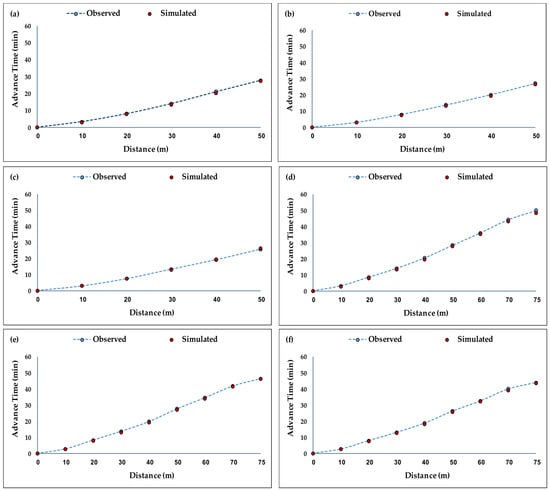
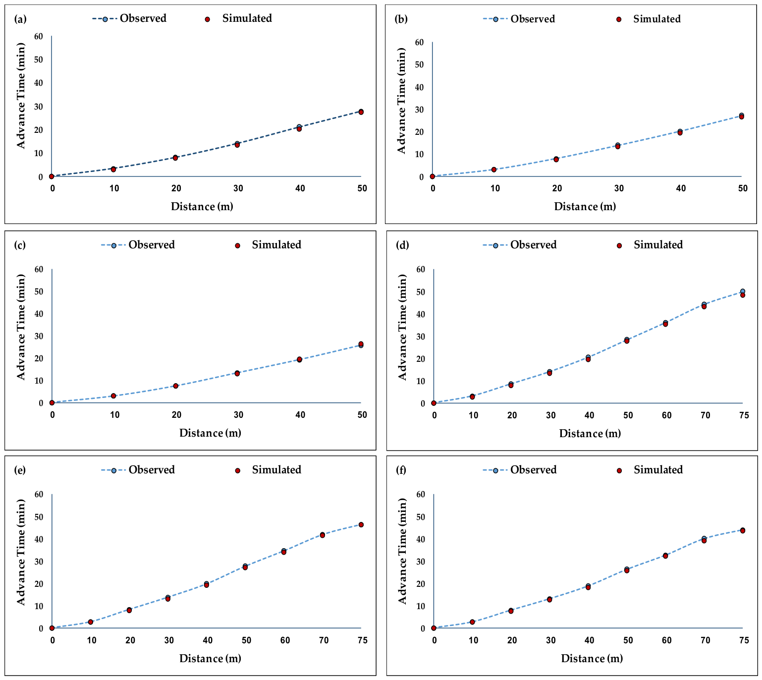
To assess how accurately the WinSRFR model predicts advance times, field-measured data were compared against model-generated outputs across all treatment combinations, as illustrated in Figure 1a–f. Analysis of variance of the advance time dataset demonstrated that FL exerted a strongly significant influence (F = 245.6, p < 0.001). A statistically significant effect was also observed for LS (F = 4.5, p < 0.05), but the combination of FL and LS was not significant (F = 1.67, p > 0.05). A concise overview of the statistical assessment for the advance time simulations is presented in Table 2.

Four statistical measures were used to evaluate the model’s performance: percent bias (PBIAS), root mean square error (RMSE), Nash–Sutcliffe efficiency (NSE), and coefficient of determination (R²). R² and NSE should be close to 1.0, RMSE should be near zero, and PBIAS should be near zero for a perfect model fit, showing little systematic over- or under-prediction. The statistical evaluation results for advance time simulation are summarized in

Table 3. Statistical evaluation of WinSRFR model performance for advance time, recession time and infiltration depth simulation.

Furrow Length	Slope	Advance Time (min)				Recession Time (min)				Infiltration (mm)
		R2	RMSE	NSE	PBIAS	R2	RMSE	NSE	PBIAS	R2	RMSE	NSE	PBIAS
50 m	0%	0.99	0.42	0.99	−1.8	0.96	0.83	0.816	−1.17	0.98	1.27	0.988	−1.36
	0.05%	0.99	0.45	0.99	−2.1	0.91	1.29	0.223	−5.19	0.99	0.91	0.993	−4.85
	0.15%	0.99	0.48	0.99	−2.99	0.9	1.09	0.508	−3.47	0.99	0.54	0.997	−0.59
75 m	0%	0.99	0.55	0.99	0.5	0.98	0.97	0.912	−1.10	0.99	1.29	0.997	−1.60
	0.05%	0.99	0.52	0.99	−1.2	0.87	1.21	0.432	−3.17	0.99	1.31	0.995	−1.13
	0.15%	0.99	0.50	0.99	−2.5	0.97	0.98	0.802	−2.21	0.99	0.84	0.998	−0.70

.

In all LS situations, the model showed good agreement with field observations for the 50 m FL treatments. The simulated values (2.91, 7.63, 13.43, 20.06, and 27.39 min) nearly matched the observed advance times (3.3, 8.0, 14.0, 21.0, and 27.8 min at distances of 10, 20, 30, 40, and 50 m, respectively) at 0% LS. Similar to the observed data, the generated advance curves for 0.05% and 0.15% LSs showed a similar pattern, with a minor underestimation in the mid-furrow area (20–40 m). This pattern is in line with research by [9,30], who found that the simplified description of infiltration dynamics causes WinSRFR to somewhat underestimate progress times in clay loam soils during the mid-furrow phase.

The model performed comparably well for the 75 m FL treatments. The measured advance times (3.1, 8.5, 14.0, 20.5, 28.3, 36.1, 44.3, and 50.0 min) under 0% LS were precisely reproduced by simulations (2.66, 7.97, 13.42, 19.62, 27.87, 35.34, 43.30, and 48.28 min). The 0.05% and 0.15% LS treatments also showed a high degree of agreement; the 0.15% LS gave the fastest advance times (observed: 2.65, 7.9, 13.0, 18.8, 26.2, 32.6, 40.0, and 44.0 min; simulated: 2.59, 7.57, 12.59, 18.2, 25.57, 32.17, 39.13, and 43.47 min). The observed pattern of faster water advance with increasing LS is hydraulically coherent because higher slopes increase flow velocity and decrease resistance.

As shown in Table 3, the statistical evaluation confirmed the model’s high predictive capability. R² values reached 0.99 for all treatments, indicating that 99% of the variability in observed advance times was explained by the simulated values. The RMSE ranged from 0.42 to 0.55 min (approximately 25 to 33 s), representing less than 2% of the total advance time, which is considered excellent for surface irrigation modeling. NSE values were consistently 0.99, demonstrating that the model predictions were superior to using the mean observed values as a baseline predictor. PBIAS values ranged from −2.99% to +0.5%, indicating negligible systematic bias, with slight underestimation observed primarily under the steeper slope conditions (PBIAS = −2.99% for 50 m with 0.15% LS).

These statistical findings align with previous validation studies of WinSRFR. According to [30], the RMSE and NSE values for advance time simulation in sugarcane fields with furrow irrigation varied from 3.64 to 13.7 min and 0.87 to 0.99, respectively. Additionally, Ref. [9] demonstrated that when growing sunflowers with varying FLs and input rates, WinSRFR was highly similar to what was observed in the field (R² > 0.93, RMSE 1.4%). The careful calibration of infiltration parameters (k = 108–112 mm hr^−a, a = 0.29–0.31) and Manning’s roughness coefficient (n = 0.05) for the clay loam soil conditions is responsible for the improved performance seen in this study (R² = 0.99, RMSE < 0.55 min). The high accuracy of the WinSRFR model in simulating advance times has important implications for sustainable irrigation management. Water application efficiency and deep percolation losses are directly impacted by accurate cutoff time prediction made possible by accurate water advance simulation. Radmanesh et al. [31] reported, based on a study in a cropped field, that simulation models can help farmers schedule irrigation more effectively, save water, and potentially sustain or enhance crop yields under cultivated conditions. Sustainable farming is closely connected to multiple Sustainable Development Goals, particularly Goal 2 (zero hunger) along with Goal 6 (clean water and sanitation). The validated WinSRFR model offers useful support for irrigation extension services in their policy-related decision-making. Policy-makers, through simulated advice on optimal FL and LS configurations, can incentivize farmers to adopt laser leveling and better furrow designs. This is especially true in Egypt, where a lack of water and small, broken-up landholdings make it hard to keep farming going [32].

3.2. Model Performance Evaluation for Recession Time Simulation

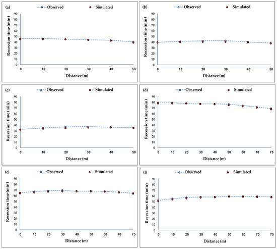
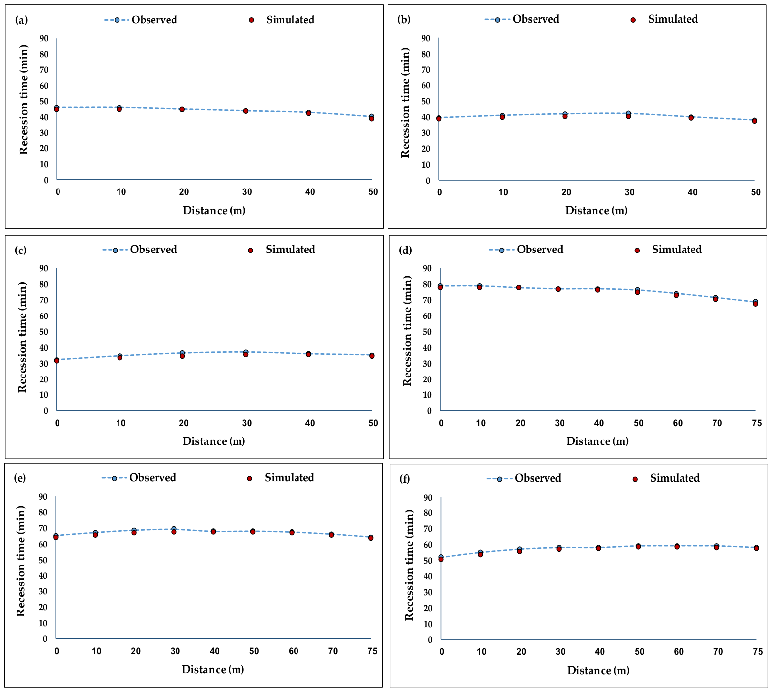
The ability of the WinSRFR model to predict recession times was evaluated by comparing field-observed data with simulated results across every treatment combination, which is displayed in Figure 2a–f. Based on the ANOVA for recession time, FL had a considerable effect (F = 189.3, p < 0.001), and LS also showed a high effect (F = 12.0, p < 0.01), whereas their combination did not reach statistical significance (F = 0.67, p > 0.05). The statistical evaluation results for recession time simulation are summarized in Table 3.

Recession time is the amount of time it takes for water to fully soak into or drain from the soil surface after the inflow has stopped. It is an important factor for figuring out how much water is lost through deep percolation and how well water is applied. Advance time is mostly controlled by the rate of inflow and the shape of the furrow. Recession time, on the other hand, is more affected by differences in soil infiltration properties and micro-topography, which makes it harder to simulate accurately.

The model achieved an R² of 0.96 for the 50 m FL with a 0% LS. This means that 96% of the differences in observed recession times could be explained by the simulated values. The RMSE was 0.83 min, which is less than 2% of the total time of the recession. This is great for modeling surface irrigation. The model predictions outperformed the mean observed value as a predictor, as evidenced by the NSE value of 0.816. Because the model assumes uniform soil qualities, the PBIAS of −1.17% shows a tiny underestimating of recession periods that is hydraulically consistent. However, actual field circumstances usually show slight spatial variability that can delay recession locally. This result is consistent with [31], who found that under uniform LS settings, recession time models are typically more accurate because of the decreased hydraulic complexity. The model displayed a different pattern for the 50 m FL with a 0.05% LS. The NSE fell precipitously to 0.223, while the R² stayed high at 0.91, suggesting a strong linear association between observed and simulated values. This variation is analytically noteworthy since it shows that, despite the model’s excellent correlation with the overall trend of recession times, there were large absolute discrepancies between the simulated and observed numbers. The PBIAS reached −5.19%, the greatest underestimate of any treatment, while the RMSE rose to 1.29 min. The hydraulic behavior of water during the recession phase is responsible for this noticeable underestimation under mild LS conditions. Water tends to collect in micro-depressions along the furrow on a 0.05% LS, resulting in small areas of stagnant water that drain slowly. Recession times are consistently underestimated because the WinSRFR model, which is predicated on a smooth, continuous furrow bed, is unable to adequately account for these micro-topographic impacts. This interpretation is supported by [30], who observed that model accuracy for recession time decreases under gentle slopes due to increased surface storage effects.

The model showed markedly better performance for the 50 m FL under the 0.15% LS treatment compared with the 0.05% LS condition, recording an R² value of 0.90 and an NSE of 0.508. In addition, the PBIAS reached −3.47%, while the RMSE was 1.09 min. The improved accuracy observed under steeper slope conditions may be attributed to the enhanced drainage behavior within the furrow system. At a 0.15% LS, gravitational forces become more dominant than capillary and surface tension forces, thereby reducing the influence of small-scale surface irregularities on recession timing. As a result, water movement becomes more uniform, making the recession phase easier for the model to simulate accurately. This observation aligns with hydraulic principles indicating that steeper slopes enhance model reliability by reducing the relative effect of localized surface water storage. Gupta et al. [9,18] reported similar findings, noting that WinSRFR performs better for recession time simulation under steeper slopes where gravitational flow dominates. For the 75 m FL at an LS of 0%, the model demonstrated the best performance among all treatments, with an R² of 0.98, an NSE of 0.912, and an RMSE of only 0.97 min. The PBIAS of −1.10% indicates negligible systematic bias. The superior performance for this treatment is analytically important for two reasons. First, the longer FL (75 m) lessens the impact of localized measurement mistakes by providing more data points for model calibration (nine measurement stations as opposed to six for 50 m furrows). Second, in zero-slope settings, infiltration rather than gravitational drainage drives the recession process, resulting in a more spatially uniform pattern that the model can more accurately depict. This result is in line with the findings of [30], who noted that when FL increases, model accuracy increases as relative measurement error decreases. For the 75 m FL at an LS of 0.05%, the model achieved an R² of 0.87 and an NSE of 0.432, with an RMSE of 1.21 min and a PBIAS of −3.17%. Similar to the 50 m case with 0.05% LS, the substantial difference between R² (high) and NSE (moderate) indicates that while the model captured the overall recession trend, absolute prediction errors were more significant. The longer FL amplified the effect of gentle slope on recession dynamics. At 75 m, water must travel a greater distance to drain, creating more opportunities for micro-topographic variations to influence recession timing. The model’s assumption of uniform soil infiltration along the entire FL becomes increasingly problematic as FL increases under gentle LS conditions, explaining the moderate NSE value despite the high R².

The model demonstrated strong performance at a 75 m FL at an LS of 0.15%, with a coefficient of determination (R²) of 0.97 and a Nash–Sutcliffe efficiency coefficient (NSE) of 0.802, indicating that the model’s predictions explained 80% of the variance in observed recession timings. The root mean square error (RMSE) was 0.98 min, while the relative bias of error (PBIAS) was −2.21%. Combining a longer FL and a steeper LS appears to improve model performance. Where the longer length provides more data points for calibration, while the steeper slope reduces the effects of surface storage, thus simplifying soil retreat. This synergistic effect is analytically important because it suggests that the optimal conditions for model accuracy (longer furrows, steeper slopes) align with the optimal conditions for irrigation efficiency identified in earlier sections of this study. Specifically, the 75 m FL at an LS of 0.15% provided the most reliable recession time predictions, while the 50 m FL at an LS of 0.15% achieved the best overall hydraulic performance. An interesting analytical pattern was found when several treatments were compared. In comparison to treatments with a 0.05% LS (0.223 for 50 m and 0.432 for 75 m), treatments with a 0% LS (0.816 for 50 m and 0.912 for 75 m) consistently recorded higher Nash–Sutcliffe efficiency coefficient (NSE) values. This suggests that LS has a major impact on how accurately the model predicts the recession time, with 0% LS conditions yielding the best accurate predictions. The 0.15% LS treatments, on the other hand, produced intermediate NSE values (0.508 for 50 m, 0.802 for 75 m), indicating that steeper slopes reduce but do not totally remove the prediction errors linked to moderate slopes. Practical ramifications for irrigation management result from the systematic underestimating of recession times across all treatments (negative PBIAS values ranging from −1.10% to −5.19%). The model may indicate that water has completely drained from the soil surface earlier than really happens if it underestimates the recession time. If farmers solely depend on model projections without field validation, this could result in early recommendations for upcoming irrigation events, thereby leading to water stress. As a result, even while the model is useful for comparing various treatments, its absolute recession time forecasts should be evaluated cautiously, especially in situations with moderate slopes where underestimating is most noticeable. The high accuracy of the WinSRFR software in simulating recession times under zero and steeper slope conditions has important implications for sustainable irrigation management. Precise calculation of deep percolation losses and water application efficiency, which are essential for optimizing irrigation scheduling in water-scarce areas, is made possible by accurate recession time prediction. Through accurate modeling of the irrigation advance and recession stages, water managers can identify the ideal moment to terminate irrigation, thereby reducing water waste and maintaining adequate soil moisture for plant development under cultivated conditions [31]. This directly supports the Sustainable Development Goals for sustainable agriculture, particularly Goal 6 (clean water and sanitation) by reducing water waste, and Goal 2 (zero hunger) by maintaining or increasing agricultural productivity. From a policy standpoint, farmers can optimize cutoff times depending on field-specific conditions by integrating the verified WinSRFR model for recession time simulation into irrigation consulting services. However, local field validation should be added to model suggestions, especially in regions where 0.05% LSs are typical, given the found underestimate bias under mild slopes. Such decision-support tools can encourage the adoption of better irrigation techniques while recognizing the limitations of model predictions under particular topographic conditions in Egypt, where water scarcity and fragmented landholdings pose serious challenges to agricultural sustainability [32].

3.3. Model Performance Evaluation for Infiltration Depth Simulation

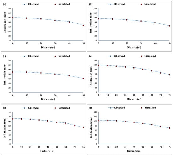
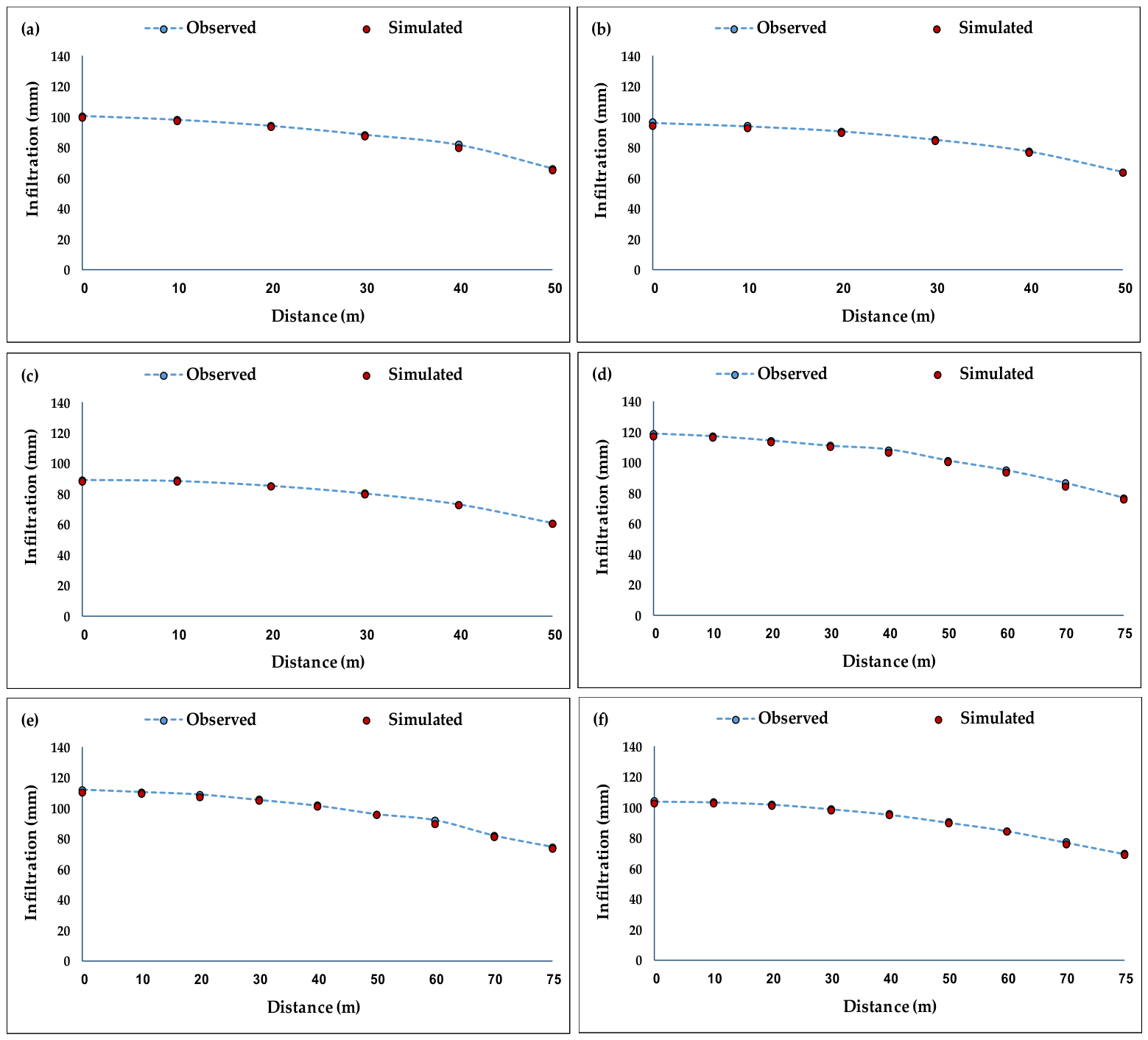
Figure 3a–f shows a comparison between simulated and actual cumulative infiltration depths for all treatment combinations, which was used to evaluate the ability of the WinSRFR model to predict infiltration. The ANOVA conducted on infiltration depth measurements demonstrated that FL exerted an extremely pronounced influence (F = 98.8, p < 0.001). LS also produced a notable effect (F = 7.32, p < 0.05), whereas the interaction between the two factors did not reach statistical significance (F = 0.48, p > 0.05). The statistical evaluation results for infiltration depth simulation are summarized in Table 3.

Infiltration amount serves as a key indicator for assessing deep percolation losses, irrigation efficiency, and water retention within the crop root zone, which is the amount of water that seeps into the soil profile per unit area along the FL. Infiltration depth is particularly sensitive to spatial variability in soil texture, initial moisture content, and furrow geometry because it directly reflects the combination between applied water and soil hydraulic properties, unlike advance and recession times, which characterize the surface hydraulics of water flow. The statistical evaluation results for the infiltration depth simulation are summarized in Table 3.

The model showed outstanding agreement with field measurements at every measurement point for the 50 m furrow 50 m FL at an LS of 0%. The diminishing opportunity time for infiltration as water moves down the furrow is reflected in the observed infiltration depths, which gradually declined from 100.5 mm at the furrow head (0 m) to 66.0 mm at the tail (50 m). This pattern is hydraulically consistent, tail regions have shorter soaking times because water arrives later, whereas spots nearer the furrow head are buried for longer periods of time, allowing more water to permeate. With an R² value of 0.988, which shows that the simulated values accounted for 98.8% of the variation in observed infiltration depths, the statistical examination validated the model’s strong predictive capacity. For surface irrigation modeling, the RMSE of 1.27 mm, or less than 2% of the total infiltration depth, is outstanding. While the PBIAS of −1.36% shows minimal systematic underestimating, the NSE value of 0.988 reveals that the model predictions were better than utilizing the average recorded value for prediction purposes. Interestingly, the model mistakes were mostly random rather than systematic, with no discernible bias in the direction or size of predictions, according to the equality of R² and NSE (both 0.988).

The measured infiltration depths, varying between 96.1 mm near the upstream end and 63.7 mm toward the downstream end, were uniformly smaller for the 50 m furrow combined with a 0.05% LS compared to those recorded under a 0% LS. This decrease in infiltration is explained by the quicker water advance in sloping settings, which shortens the amount of time that water has to seep into the soil at any one location along the furrow. The model obtained an NSE of 0.993, an RMSE of 0.91 mm, and an R² of 0.993. A modest systematic underestimating of infiltration under mild slope conditions is suggested by the PBIAS of −4.85%, which was marginally higher than for other treatments. Despite this, the equality of R² and NSE (both 0.993) indicates that the model captured the spatial pattern of infiltration along the furrow with remarkable consistency, and the underestimation was uniform rather than varying systematically with distance. This underestimation may be attributed to the model’s difficulty in fully capturing the complex combination between flow velocity and infiltration dynamics when water advance is accelerated by even a small slope gradient.

For a 50 m FL at an LS of 0.15%, the reported infiltration depths, ranging from 89.1 mm at the start to 60.7 mm at the end, were the lowest among the three LS treatments. A steeper slope accelerates water movement, reducing cumulative infiltration along the entire furrow by decreasing opportunity time. With an R² of 0.997, an RMSE of just 0.54 mm (less than 1 mm), and an NSE of 0.997, this therapy outperformed all other 50 m treatments statistically. The PBIAS of −0.59% indicates nearly perfect agreement between observed and simulated values, with negligible systematic bias. The equality of R² and NSE (both 0.997) demonstrates that the model’s predictions were both well-correlated and accurate in absolute terms. This high level of accuracy indicates that the Kostiakov infiltration parameters (k = 108–112 mm hr^−a, a = 0.29–0.31) were particularly well-calibrated for the clay loam soil conditions under steeper slopes, where gravitational forces dominate over capillary effects. The pattern of decreasing infiltration with increasing slope observed across the three 50 m treatments is analytically significant. Head-section infiltration dropped from 100.5 mm at 0% LS to 96.1 mm at 0.05% LS (a 4.4% decline) and then to 89.1 mm at 0.15% LS (an 11.3% decrease from the baseline at 0% LS). With higher slopes decreasing infiltration at the furrow head and possibly increasing distribution uniformity over the FL, this trend shows that LS gradient directly affects water distribution patterns. The high R² and NSE values for each of the three slope treatments show that the model was successful in capturing this steady decrease in infiltration with increasing slope. With values ranging from 118.6 mm at 0 m to 76.6 mm at 75 m, the observed infiltration depths for the 75 m FL with 0% LS displayed a similar decreasing pattern from head to tail. The longer FL, which results in a greater cumulative water volume supplied to the upstream areas during the advance phase, is reflected in the higher infiltration depths at the head when compared to the 50 m furrow treatment. The statistical analysis revealed a PBIAS of −1.60%, an R² of 0.997, an RMSE of 1.29 mm, and an NSE of 0.997. The model’s small and impartial mistakes are confirmed by the equivalence of R² and NSE (both 0.997). Given the larger number of measurement points (9 vs. 6) and the longer FL, which adds more spatial variability in infiltration patterns, the slightly higher RMSE (1.29 mm vs. 0.54–1.27 mm) in comparison to the 50 m treatments is expected.

The observed infiltration depths for the 75 m FL with a 0.05% LS varied from 112.0 mm at the head to 74.5 mm at the tail. The combined impact of longer FL and mild LS on water advance dynamics is reflected in the decrease in infiltration as compared to the 0% LS treatment (a decrease of roughly 5.6% at the head). With a PBIAS of −1.13%, the model obtained an R² of 0.995, an RMSE of 1.31 mm, and an NSE of 0.995. The model’s predictions were accurate and well-correlated, as evidenced by the equality of R² and NSE (both 0.995). The slightly lower R² and NSE (0.995 vs. 0.997) in comparison to the 0% LS treatment indicate that the mild slope adds some more complexity to infiltration patterns, which the model nonetheless captures with a high degree of accuracy.

The combination of a 75 m FL and a 0.15% LS yielded the smallest infiltration amounts, where recorded infiltration depths varied between 104.0 mm near the upstream end and 69.3 mm toward the downstream end. The most uniform infiltration distribution along the furrow was achieved by combining a longer FL with a steeper LS; the disparity between head and tail infiltration was reduced to about 35 mm instead of 42 mm under 0% LS conditions. This therapy performed significantly better than all other 75 m treatments, with an R² of 0.998, an RMSE of 0.84 mm, an NSE of 0.998, and a PBIAS of −0.70%. The model is especially well-suited for predicting infiltration under steeper slope conditions, where flow is more uniform and gravitational forces predominate over surface storage effects, as confirmed by the excellent agreement between observed and simulated values and the equality of R² and NSE.

By comparing the statistical results between the treatments, several significant patterns emerge. First, independent of FL or LS condition, the model accurately depicted the general trend of decreasing infiltration from head to tail, with R² values consistently above 0.98 across all treatments. Second, the RMSE values were consistently less than 1.5 mm, with the 0.15% LS treatments showing the lowest values (0.54 mm for 50 m and 0.84 mm for 75 m). This indicates that the model’s accurate prediction increases with slope, probably because micro-topographic differences have less of an impact on water distribution on steeper slopes. Third, there was no discernible bias in the direction or size of predictions, and the NSE values were almost the same as the R² values for every treatment, suggesting that the model’s errors were mostly random rather than systematic. Fourth, the PBIAS values were consistently negative but small in magnitude (varying from −0.59% to −4.85%), suggesting a persistent underestimating of infiltration depths that is particularly noticeable when the slope is moderate.

The high accuracy in the prediction of the infiltration depth using WinSRFR will have important repercussions on irrigation management practices. Estimation of the moisture storage capability of the soil within the root zone can be achieved through precise estimation of the depth of infiltration, an aspect that plays a critical role in optimizing irrigation practices and minimizing deep percolation loss. Irrigation managers will benefit from accurate modeling of the depth of infiltration along the entire length of the furrow to determine ideal combinations of LS and FL. According to [33], correct prediction of cumulative infiltration as a function of opportunity time is crucial for increasing irrigation efficiency, and infiltration characteristics are key to surface irrigation analysis and design.

From a policy perspective, the validated WinSRFR model for infiltration simulation can inform decisions about irrigation system design and water allocation in water-scarce regions. In Egypt, the combination of water scarcity and fragmented land ownership poses serious obstacles to sustainable agriculture [32]. Simulation tools like the one validated in this study can assist in designing more efficient new irrigation schemes and enhancing existing ones, thereby advancing national water-saving objectives and contributing to global development targets, specifically those related to clean water (Goal 6) and food security (Goal 2).

3.4. Performance Indicators of Furrow Irrigation

Water distribution uniformity (DU), water application efficiency (AE), and deep percolation (DP) were the three key indicators employed to evaluate the performance of furrow irrigation across the various treatments of FL and LS. These indicators collectively determine the effectiveness of irrigation management and directly influence water productivity and sustainability of agricultural systems. Based on the ANOVA performed for the performance indicators, FL produced a statistically very strong effect on DU (F = 89.4, p < 0.001), AE (F = 156.3, p < 0.001), and DP (F = 367.9, p < 0.001). Land slope also exhibited an exceptionally significant influence on all three indicators, with F-values spanning from 23.4 to 56.3 (p < 0.001). The combined effect of FL with land slope proved significant for AE (F = 4.1, p < 0.05) and DP (F = 4.1, p < 0.05), whereas it was not significant for DU (F = 2.4, p > 0.05). An overview of these results is presented in

Table 4. Hydraulic performance indicators for furrow irrigation under varying furrow lengths and slopes.

Furrow Length	Slope	Water Distribution Uniformity (%)		Water Application Efficiency (%)		Deep Percolation (%)
		Observed	Simulated	Observed	Simulated	Observed	Simulated
50 m	0%	85.0 ± 0.58 C	85	84.0 ± 0.58 B	84	11.0 ± 0.12 C	10.6
	0.05%	88.0 ± 0.58 B	85	86.0 ± 0.58 A	86	9.0 ± 0.06 B	7
	0.15%	90.0 ± 0.58 A	86	87.0 ± 0.58 A	89	6.0 ± 0.15 A	4
75 m	0%	79.0 ± 0.58 F	84	74.0 ± 0.58 E	72	24.0 ± 0.88 F	22
	0.05%	83.0 ± 0.58 E	85	78.0 ± 0.58 D	76	15.0 ± 0.58 E	18
	0.15%	86.0 ± 0.58 D	85	82.0 ± 0.58 C	80	12.0 ± 0.58 D	14

Data are presented as the mean of three replicates ± standard error (SE). According to Duncan’s Multiple Range Test at p < 0.05, means in the same column that are marked with different letters (A–F) are statistically different, while those with the same letter are not.

.

3.4.1. Water Distribution Uniformity (DU)

The DU along the length of the furrow is reflected in water distribution uniformity. In order to achieve uniform water distribution (which is essential for crop growth and to minimize potential water stress at the tail end of furrows), more uniform water application is indicated by higher DU values. The observed DU values ranged from 79% for the 75 m long furrow with a 0% LS to 90% for the 50 m long furrow with a 0.15% LS. Across all treatments, the DU values showed a clear pattern: shorter furrows (50 m) achieved higher uniformity (85–90%) than longer furrows (75 m), which ranged from 79% to 86% Table 4. Because lengthier furrows encounter more variability in infiltration opportunity time along their length, resulting in an uneven distribution at the downstream end, this pattern is hydraulically consistent.

In the context of LS’s impact, DU was enhanced for both FLs when LS was increased from 0% to 0.15%. The DU for the 50 m furrow increased by 5.9%, from 85% at 0% LS to 90% at 0.15% LS, while the DU for the 75 m furrow increased by 8.9%, from 79% at 0% LS to 86% at 0.15% LS. The faster water movement under steeper slopes, which shortens the time available for differential infiltration over the FL, is responsible for this improvement. Similar increases in DU under ideal furrow irrigation conditions were reported by [9]. Even the highest DU values (90% for 50 m with 0.15% LS), however, are still within the 91–94% range recorded under alternate furrow irrigation, indicating that more inflow rate and cutoff timing optimization may improve uniformity.

3.4.2. Water Application Efficiency (AE)

The term water application efficiency (AE) describes how much of the water applied through irrigation stays in the root zone and remains usable for plant uptake in cropped fields.

According to [34], higher AE values signify more effective irrigation water utilization, which is essential for sustainable agriculture in water-scarce areas. The 50 m furrow with a 0.15% LS had an AE value of 87%, whereas the 75 m furrow with a 0% LS had an AE value of 74%. AE was consistently higher for shorter furrows (50 m) than for longer furrows (75 m), much like DU. AE improved by 3.6% for the 50 m furrow, rising from 84% at 0% LS to 87% at 0.15% LS. AE improved by 13.5% for the 75 m FL, rising from 74% at 0% LS to 84% at 0.15% LS. Slope modification is especially important for reducing the efficiency losses related to longer furrows, as evidenced by the more noticeable improvement for longer furrows. The AE values recorded in the present study (84 to 87% for 50 m furrows) are consistent with those reported by [9,18], who obtained an application efficiency of 87% under alternate furrow irrigation using optimized operating conditions. In contrast, the AE observed for the 75 m FL under a 0% LS condition (74%) was lower than the range generally regarded as acceptable for modern irrigation systems. This finding underscores the importance of integrating suitable FLs with appropriate slope design to achieve efficient irrigation performance.

The relationship between AE and slope can be explained by the balance between water advance time and infiltration opportunity. Water moves more quickly under steeper slopes, ensuring that enough water reaches the tail while decreasing the amount of time available for profound percolation at the furrow head. Achieving the right slope is essential, as excessive steepness may lead to surface runoff, whereas insufficient slope can cause deep percolation near the furrow inlet and inadequate water supply toward the downstream end, as demonstrated by Park et al. [35].

3.4.3. Deep Percolation (DP)

The fraction of irrigation water that infiltrates below the root zone and thus becomes inaccessible to the crop is called “deep percolation”. Inefficient water use and possible groundwater contamination are indicated by high DP values. For the 50 m furrow with a 0.15% LS and the 75 m furrow with a 0% LS, the observed DP values varied from 6% to 24%.

FL and LS showed a substantial inverse connection with DP. In comparison to larger furrows (75 m), which ranged from 12% to 24%, shorter furrows (50 m) regularly displayed lower DP (6–11%). This pattern shows that when the FL is shorter, there is less time for water to penetrate below the root zone. Slope had a similarly noticeable impact on DP. DP dropped by 50% for the 75 m furrow, from 24% at 0% LS to 12% at 0.15% LS. This significant improvement shows how important LS is in reducing deep percolation losses, especially for longer furrows.

The 6% DP value recorded for the optimal treatment (50 m FL with a 0.15% LS) is consistent with values reported in previous studies. For instance, with optimal alternate furrow irrigation, Shah et al. and Gupta et al. [9,10] reported deep percolation of about 15%. The low DP values found in this study show that water losses can be successfully reduced while keeping high uniformity and efficiency when laser levelling, optimal FL, and suitable slope selection are combined. It is important to note very low DP values (below 5%) may indicate inadequate irrigation, which could potentially lead to water stress at the end of the field under cropped conditions. The high AE (87%) and DU (90%) values in this study suggest that the 6% DP achieved for a 50 m furrow with a 0.15% LS represents an ideal equilibrium.

3.4.4. Integration of Performance Indicators

This combination is consistent with findings from cropping studies [31], suggesting a potential relationship between hydraulic performance and crop productivity under field conditions. Conversely, the lowest performance across all indicators was recorded for the treatment combining a 75 m FL and a 0% LS, yielding DU of 79%, AE of 74%, and DP of 24%. This highlights the need for appropriate furrow design for crop productivity and hydraulic efficiency. Although the 50 m furrow with 0.15% LS remained superior, the significant improvements obtained by increasing LS from 0% to 0.15% for the 75 m FL (AE increased by 8 percentage points (from 74% to 82%), DP decreased by 50%) show that LS optimization can partially offset the negative effects of longer FLs.

3.4.5. Comparison Between Observed and Simulated Values

The comparison of observed and simulated results provides valuable insight into the predictive accuracy of the model. For distribution uniformity (DU), the model demonstrated strong agreement with the measured data for the 50 m furrow treatments, where simulated values (85 to 86%) were very close to the observed values (85 to 90%), with deviations remaining below 4%.

For the 75 m furrow treatments, however, the model tended to overpredict DU under the 0% and 0.05% LS conditions, with simulated values ranging from 84 to 85% compared with observed values of 79 to 83%. In contrast, a slight underestimation was noted for the 0.15% LS treatment, where the simulated DU value was 85% versus an observed value of 86%. These findings indicate that the WinSRFR model may have limited capability in fully representing the greater variability in water distribution associated with longer FLs, especially under level and mildly sloping field conditions [18].

For AE, the model demonstrated high accuracy for the 50 m furrow treatments, where simulated values (84–89%) were within 1–2% of observed values (84–87%). For the 75 m furrow treatments, however, the model consistently underestimated AE, with simulated values (72–80%) being 4–6% lower than observed values (78–84%). This systematic underestimation for longer furrows suggests that, given the clay loam soil conditions of the research location, the model’s infiltration parameters may need to be recalibrated for FLs longer than 50 m.

For DP, the model showed good agreement for the 75 m furrow treatments, where simulated values (14–22%) were within 2–3% of observed values (12–24%). However, for the 50 m furrow treatments, the model consistently underestimated DP, with simulated values (4–10.6%) being 0.4–3% lower than observed values (6–11%). This pattern suggests that the model may overestimate the efficiency of water retention in shorter furrows, potentially due to simplified representation of root zone storage capacity.

The observed discrepancies between measured and simulated performance indicators highlight the importance of field validation for model-based recommendations. While WinSRFR proved highly reliable for simulating advance times (R² > 0.99) and infiltration depths (R² > 0.98), its accuracy for predicting AE and DP was somewhat lower for longer FLs. These findings align with [30], who noted that model accuracy decreases with increasing FL due to cumulative errors in infiltration parameter estimation. Therefore, while WinSRFR is a valuable tool for comparative analysis and optimization, its absolute predictions should be interpreted with caution, particularly for FLs exceeding 50 m in clay soils.

3.4.6. Implications for Sustainable Water Management

The performance indicators evaluated in this study have direct implications for sustainable water management and policy development. The high DU and AE values achieved under optimal combinations (50 m FL at an LS of 0.15%) demonstrate that properly designed furrow irrigation systems can achieve efficiency levels comparable to more advanced irrigation technologies. This is particularly significant in developing countries where smallholder farmers may lack the capital to invest in pressurized irrigation systems, as noted by [34].

The findings emphasize the significance of encouraging laser levelling technology and giving farmers advice on the ideal furrow dimensions from a policy standpoint. According to [36], focused extension programs may result in large water savings at the national level because of the significant improvements made possible by very inexpensive interventions like laser levelling and optimized furrow design. Additionally, under ideal circumstances, the decreased deep percolation losses (6–12%) suggest a lower chance of agrochemical contamination of groundwater, supporting environmental sustainability objectives.

It is notable that these results correlate with the Sustainable Development Goals (SDGs). Reduced water loss and increased irrigation efficiency directly help SDG 6 (clean water and sanitation). The potential for increased crop productivity and yield stability (under cropped conditions) would help achieve SDG 2 (zero hunger). More resilient agricultural systems that can adjust to growing water scarcity help achieve SDG 13 (climate action). According to [34,35], integrating performance-based irrigation design with sustainability goals offers a framework for evidence-based policy-making that can direct investments in agricultural water management.

4. Conclusions

The hydraulic performance of furrow irrigation on clay loam soils was investigated using field measurements and WinSRFR modeling, with FLs set at 50 and 75 m and land LSs at 0%, 0.05%, and 0.15%. The 50 m furrows consistently exceeded the 75 m furrows across all performance measures, demonstrating that FL has a substantial influence on all hydraulic parameters. In comparison to 75 m furrows, which recorded DU of 79–86%, AE of 74–82%, and DP of 12–24%, the 50 m furrows achieved higher water distribution uniformity (85–90%), higher water application efficiency (84–87%), and reduced deep percolation losses (6–11%). Increasing the LS from 0% to 0.15% improved all hydraulic parameters for both FLs, indicating that LS was crucial in enhancing irrigation efficacy. Slope optimization is especially crucial for longer furrows, as evidenced by the 75 m furrow, where increasing the LS to 0.15% decreased deep percolation by 50% (from 24% to 12%) and increased application efficiency by 8 percentage points (from 74% to 82%). The best combination, which produced the highest DU (90%), highest AE (87%), and lowest DP (6%), was a 50 m FL at an LS of 0.15%.

The WinSRFR model accurately predicted advance times and infiltration depths, with R² values above 0.99 for advance times with RMSE less than 0.55 min and exceeding 0.98 for infiltration depths with RMSE less than 1.3 mm. Model performance during recessions varied considerably across treatments. For the 0% and 0.15% LS treatments, the model performed well (NSE = 0.802–0.912, R² = 0.90–0.98). However, for the 0.05% LS treatments, the model showed unsatisfactory performance (NSE = 0.223 for the 50 m furrow and NSE = 0.432 for the 75 m furrow, both below the 0.50 threshold). This suggests that recession dynamics, particularly under gentle slope conditions, are more complex to adequately replicate due to micro-topographic effects and surface storage. Model accuracy varied with treatment conditions, with WinSRFR performing better for shorter FLs (50 m) than longer FLs (75 m), and for steeper LSs (0.15%) than mild LSs (0.05%). The persistent underestimation of AE for 75 m furrows (simulated values 4–6% lower than observed) suggests that model calibration should be performed separately for each FL to attain the best accuracy.

Study Limitations: This study was conducted under specific conditions: clay loam soil, bare-soil conditions, March 2024 (single month), and a single location (Banha, Egypt). The FLs were limited to 50 and 75 m, and LSs to 0%, 0.05%, and 0.15%. Therefore, the findings may not be directly transferable to other soil types, climatic conditions, or cropped situations without further validation.

Recommendations for Future Research: To build on these findings, additional studies are necessary to confirm their applicability under different soil textures, cropped environments, long-term trials, and variable weather patterns, as well as to assess the economic feasibility of adopting optimized furrow designs at different spatial scales.

References

- Hashemi, S.Z.; Darzi-Naftchali, A.; Karandish, F.; Ritzema, H.; Solaimani, K. Enhancing agricultural sustainability with water and crop management strategies in modern irrigation and drainage networks. Agric. Water Manag. 2024, 305, 109110. [Google Scholar] [CrossRef] [Scilit]
- Perez, N.; Singh, V.; Ringler, C.; Xie, H.; Zhu, T.; Sutanudjaja, E.H.; Villholth, K.G. Ending groundwater overdraft without affecting food security. Nat. Sustain. 2024, 7, 1007–1017. [Google Scholar] [CrossRef] [Scilit]
- Boutagayout, A.; Hamdani, A.; Boutgayout, I.; Adiba, A. Towards sustainable water management in Morocco: Assessing resources, challenges, and adaptation strategies. Front. Sustain. Food Syst. 2025, 9, 1666555. [Google Scholar] [CrossRef] [Scilit]
- Amer, M.H.; Amer, M.M. Surge-Flow Irrigation as Inexpensive Technique for Water Rationalization in Nile Delta. Misr J. Agric. Eng. 2025, 42, 33–48. [Google Scholar] [CrossRef] [Scilit]
- Ward, F.A.; Potter, N.A.; Hrozencik, R.A. Managing agricultural water use in the Western United States: A search for efficient climate adaptation institutions. Agric. Water Manag. 2025, 308, 109279. [Google Scholar] [CrossRef] [Scilit]
- Li, Z.; Meng, Q.; Li, L.; Bai, Z.; Li, Y.; Liu, H.; Li, P.; Wang, T. Integrated deep vertical rotary tillage and subsurface pipe drainage techniques for sustainable soil salinization management and cotton production in arid regions. Agric. Water Manag. 2025, 312, 109429. [Google Scholar] [CrossRef] [Scilit]
- Sayed, A.A.; El-Bagoury, K.F.; Hassan, S.S.; Abdou, S.H. Irrigation efficiency for the modified irrigation system under different line lengths in the Egyptian old valley. Misr J. Agric. Eng. 2024, 41, 113–124. [Google Scholar] [CrossRef] [Scilit]
- Khalifa, R.M.; Shabana, M.M.A. Furrow irrigation design and evaluation for enhancing indices of water usage performance and productivity of canola crop in North Nile Delta soils. Environ. Biodivers. Soil. Secur. 2024, 8, 51–71. [Google Scholar] [CrossRef] [Scilit]
- Gupta, A.; Rao, K.R.; Rajwade, Y.A.; Randhe, R.D.; Singh, K.; Kumar, M.; Singh, R.K. Optimizing furrow irrigation performance with WinSRFR software through field experiments and simulations in sunflower cultivation. Sci. Rep. 2025, 15, 33884. [Google Scholar] [CrossRef] [Scilit] [PubMed]
- Shah, M.A.; Waseem, M.; Iqbal, M.; Nabi, G.; Tariq, M.A.U.R.; Arshed, A.B.; Sultan, U.; Laraib, M.; Abbas, K. Improving Irrigation Performance of Raised Bed Furrow Using WinSRFR Model. Water Conserv. Sci. Eng. 2024, 9, 44. [Google Scholar] [CrossRef] [Scilit]
- Garelnabi, M.A.; Mohammed, H.I. Improving furrow irrigation performance using Skogerboe models of continuous flow for different soil. J. Agric. Res. Adv. 2024, 6, 33–41. [Google Scholar]
- Bautista, E.; Schlegel, J.L. Estimation of infiltration and hydraulic resistance in furrow irrigation, with infiltration dependent on flow depth. Trans. ASABE 2017, 60, 1873–1884. [Google Scholar] [CrossRef] [Scilit]
- Valipour, M.; Montazar, A.A. Optimize of all effective infiltration parameters in furrow irrigation using Visual Basic and genetic algorithm. J. Agric. Sci. 2012, 4, 123–132. [Google Scholar]
- Ebrahimian, H.; Liaghat, A.; Ghanbarian-Alavijeh, B.; Abbasi, F. Evaluation of various quick methods for estimating furrow infiltration. Biosyst. Eng. 2010, 105, 418–426. [Google Scholar] [CrossRef] [Scilit]
- Mostafazadeh, B.; Farzamnia, M. The Study of Hydraulic Performance of Furrow Irrigation Under Different Methods of Discharge Management. J. Water Soil. Sci. 2000, 4, 1–11. Available online: https://www.oalib.com/research/2863508 (accessed on 9 April 2026).
- Ashine, E.T.; Bedane, M.T.; Mengesha, A.A.; Admassu Lakewu, R.; Tadesse Kebede, H. Determination of appropriate furrow length and inflow rate for furrow irrigation practice on smallholder farmers at Omo Nada district for maize (Zea maize L.) production. Air Soil. Water Res. 2025, 18, 11786221241308144. [Google Scholar] [CrossRef] [Scilit]
- Bautista, E.; Clemmens, A.J.; Strelkoff, T.S.; Schlegel, J. Modern analysis of surface irrigation systems with WinSRFR. Agric. Water Manag. 2009, 96, 1146–1154. [Google Scholar] [CrossRef] [Scilit]
- Dewedar, O.M.; Mehanna, H.M.; El-Shafie, A.F. Validation of WinSRFR for some hydraulic parameters of furrow irrigation in Egypt. Plant Arch. 2019, 19, 2108–2115. [Google Scholar]
- Gee, G.W.; Bauder, J.W. Particle-size analysis. In Methods of Soil Analysis: Part 1 Physical and Mineralogical Methods; American Society of Agronomy: Madison, WI, USA, 1986; Volume 5, pp. 383–411. [Google Scholar] [CrossRef] [Scilit]
- Gardner, W.H. Water content. In Methods of Soil Analysis: Part 1 Physical and Mineralogical Methods; American Society of Agronomy: Madison, WI, USA, 1986; Volume 5, pp. 493–544. [Google Scholar] [CrossRef] [Scilit]
- Klute, A.; Dirksen, C. Hydraulic conductivity and diffusivity: Laboratory methods. In Methods of Soil Analysis: Part 1 Physical and Mineralogical Methods; American Society of Agronomy: Madison, WI, USA, 1986; Volume 5, pp. 687–734. [Google Scholar] [CrossRef] [Scilit]
- Elliott, R.L.; Walker, W.R. Field evaluation of furrow infiltration and advance functions. Trans. ASAE 2012, 25, 396–400. [Google Scholar] [CrossRef] [Scilit]
- Burt, C.M.; Clemmens, A.J.; Strelkoff, T.S.; Solomon, K.H.; Bliesner, R.D.; Hardy, L.A.; Howell, T.A.; Eisenhauer, D.E. Irrigation performance measures: Efficiency and uniformity. J. Irrig. Drain. Eng. 1997, 123, 423–442. [Google Scholar] [CrossRef] [Scilit]
- Merriam, J.L.; Keller, J. Farm Irrigation System Evaluation: A Guide for Management; Agricultural and Irrigation Engineering Department, Utah State University: Logan, UT, USA, 1978; Available online: https://digitalcommons.usu.edu/cee_facpub/3779 (accessed on 10 April 2026).
- Nash, J.E.; Sutcliffe, J.V. River flow forecasting through conceptual models part I—A discussion of principles. J. Hydrol. 1970, 10, 282–290. [Google Scholar] [CrossRef] [Scilit]
- Willmott, C.J.; Matsuura, K. Advantages of the mean absolute error (MAE) over the root mean square error (RMSE) in assessing average model performance. Clim. Res. 2005, 30, 79–82. [Google Scholar] [CrossRef] [Scilit]
- Moriasi, D.N.; Arnold, J.G.; Van Liew, M.W.; Bingner, R.L.; Harmel, R.D.; Veith, T.L. Model evaluation guidelines for systematic quantification of accuracy in watershed simulations. Trans. ASABE 2007, 50, 885–900. [Google Scholar] [CrossRef] [Scilit]
- Snedecor, G.W.; Cochran, W.G. Statistical Methods, 8th ed.; Iowa State University Press: Ames, IA, USA, 1989. [Google Scholar]
- Duncan, D.B. Multiple range and multiple “F” test. Biometrics 1955, 11, 1–42. [Google Scholar] [CrossRef] [Scilit]
- Mazarei, R.; Mohammadi, A.S.; Naseri, A.A.; Ebrahimian, H.; Izadpanah, Z. Optimization of furrow irrigation performance of sugarcane fields based on inflow and geometric parameters using WinSRFR in Southwest of Iran. Agric. Water Manag. 2020, 228, 105899. [Google Scholar] [CrossRef] [Scilit]
- Radmanesh, M.; Ahmadi, S.H.; Sepaskhah, A.R. Measurement and simulation of irrigation performance in continuous and surge furrow irrigation using WinSRFR and SIRMOD models. Sci. Rep. 2023, 13, 5768. [Google Scholar] [CrossRef] [Scilit]
- Salem, S.A.; MOumer, A.; Dhehibi, B.; Abda-Allah Abdallah, I.; Souissi, A.; Baum, M. Farmers’ Bottlenecks and Risks to Innovate and Adopt New Technologies in Egypt: A Systematic Review; International Center for Agricultural Research in the Dry Areas (ICARDA): Beirut, Lebanon, 2024; Available online: https://cgspace.cgiar.org/items/47afa413-70be-4aaf-8ada-fdb7852d58c1 (accessed on 15 April 2026).
- Amer, A.M. Effects of water infiltration and storage in cultivated soil on surface irrigation. Agric. Water Manag. 2011, 98, 815–822. [Google Scholar] [CrossRef] [Scilit]
- Taguta, C.; Dirwai, T.L.; Senzanje, A.; Sikka, A.; Mabhaudhi, T. Sustainable irrigation technologies: A water-energy-food (WEF) nexus perspective towards achieving more crop per drop per joule per hectare. Environ. Res. Lett. 2022, 17, 073003. [Google Scholar] [CrossRef] [Scilit] [PubMed]
- Park, S.H.; Kim, H.K.; Lee, J.Y.; Choi, J.Y. Improving wheat yield and water use efficiency through soil water-guided furrow irrigation and hydraulic simulation. Agric. Water Manag. 2025, 308, 109234. [Google Scholar] [CrossRef] [Scilit]
- Mirshadiev, M.; Fleskens, L.; van Dam, J.; Pulatov, A. Scoping of promising land management and water use practices in the dry areas of Uzbekistan. Agric. Water Manag. 2022, 200, 105000. [Google Scholar] [CrossRef] [Scilit]
Disclaimer/Publisher’s Note: The statements, opinions and data contained in all publications are solely those of the individual author(s) and contributor(s) and not of MDPI and/or the editor(s). MDPI and/or the editor(s) disclaim responsibility for any injury to people or property resulting from any ideas, methods, instructions or products referred to in the content. |
© 2026 by the authors. Licensee MDPI, Basel, Switzerland. This article is an open access article distributed under the terms and conditions of the Creative Commons Attribution (CC BY) license.