A Deep Learning Semantic Segmentation Method for Landslide Scene Based on Transformer Architecture

Abstract

Semantic segmentation technology based on deep learning has developed rapidly. It is widely used in remote sensing image recognition, but is rarely used in natural disaster scenes, especially in landslide disasters. After a landslide disaster occurs, it is necessary to quickly carry out rescue and ecological restoration work, using satellite data or aerial photography data to quickly analyze the landslide area. However, the precise location and area estimation of the landslide area is still a difficult problem. Therefore, we propose a deep learning semantic segmentation method based on Encoder-Decoder architecture for landslide recognition, called the Separable Channel Attention Network (SCANet). The SCANet consists of a Poolformer encoder and a Separable Channel Attention Feature Pyramid Network (SCA-FPN) decoder. Firstly, the Poolformer can extract global semantic information at different levels with the help of transformer architecture, and it greatly reduces computational complexity of the network by using pooling operations instead of a self-attention mechanism. Secondly, the SCA-FPN we designed can fuse multi-scale semantic information and complete pixel-level prediction of remote sensing images. Without bells and whistles, our proposed SCANet outperformed the mainstream semantic segmentation networks with fewer model parameters on our self-built landslide dataset. The mIoU scores of SCANet are 1.95% higher than ResNet50-Unet, especially.

1. Introduction

Landslide [1] is a geological phenomenon with great danger. The occurrence of landslide is caused by both natural and human factors. Natural factors mainly include terrain, lithology, geological structure, bad weather, etc. And human factors are mainly human activities that violate the laws of nature and destroy the stable conditions of slopes. Landslides cause great damage to industrial and agricultural production as well as people’s lives and properties. In severe cases, landslides even cause devastating disasters. For instance, in October 2021, landslides in Northeast and Southwest India caused massive casualties, infrastructure damage, crop damage and other serious disasters. After a landslide occurs, so as to facilitate rescue operations and ecological restoration work, it is very important to use satellite data or aerial photography data to quickly locate and estimate the area of the landslide [2]. In recent years, with the rapid development of remote sensing technology, more and more high-resolution remote sensing images [3] can be obtained. With rich information and high resolution, remote sensing images are gradually playing a more important role in various fields of national life. For example, in landslide disasters, remote sensing images are used to assess the area and extent of landslide impact. In order to identify landslide hazards and perform further analysis and processing, we need specific methods to separate and extract regions of interest from remote sensing images. At the same time, various remote sensing image vision tasks based on deep learning [4] methods have been greatly promoted and developed. Specifically, remote sensing image segmentation [5] can complete the pixel-level prediction of the image to effectively obtain image information. For landslide scenes, deep learning semantic segmentation methods accurately identify landslide areas to carry out disaster relief work. It is very suitable and great to solve the above regional positioning and area estimation.

Deep learning is used to learn the underlying distribution and representation level of sample data. The goal of deep learning is to make machines have the ability to analyze problems and learn knowledge like humans. Deep learning, a data-driven machine learning algorithm, has made outstanding progress in many fields, such as video scene [6] and vision scene [7]. However, deep learning methods have not been applied deeply enough in the field of various natural disasters. So as to achieve the effect of controlling, managing and reducing disasters, using deep learning technology [8] to predict and evaluate landslide areas can quickly and accurately obtain space disaster information. Taking landslide disasters in the Loess Plateau as the research object, to complete the regional positioning and area estimation of landslides, we used semantic segmentation technology based on deep learning to process and analyze remote sensing landslide images.

There are various segmentation methods based on deep learning. The mainstream architecture of semantic segmentation methods is the Encoder-Decoder [9] architecture. In order to obtain the high-level and low-level semantic information, we use the encoder to extract the features of the original image. At present, universal encoder networks are the Convolutional Neural Network [10] (CNN) based on convolution operation and the Transformer [11] self-attention mechanism [12]. Many experiments [13] showed that Transformer has a stronger ability than the convolutional neural network to extract image features. The strong performance of Transformer is attributed to the self-attention mechanism capturing global information. However, due to the self-attention mechanism causing the existence of high computational complexity, Transfromer is not widely used. The decoder network is used to fuse high-level and low-level semantic information [14] obtained by the encoder. In the decoder stage, through processing the low-level feature information after downsampling in the encoder stage to extract rich high-level feature semantic information, then, through related techniques, the corresponding feature information is adjusted to the resolution of the input image to complete pixel-level prediction. Currently, there are still very few pixel-level landslide labeled datasets. Due to the fact that pixel-by-pixel labeling of landslide datasets requires a lot of labor and financial costs, conducting experiments and testing effect in landslide scenarios by using deep learning semantic segmentation methods is difficult.

Faced with the above problems, the main contributions of this paper are as follows:

• We construct a landslide dataset based on landslide remote sensing Image in the Loess Plateau. We use support vector machines to annotate the remote sensing images of landslides to get preliminary label data. By image post-processing and manual correction, we obtained a well-labeled landslide dataset.
• On the existing landslide dataset, we conduct related experiments on different and representative semantic segmentation network. After that, we compare and analyze the performance of different networks.
• We propose a deep learning semantic segmentation method based on Encoder-Decoder architecture for landslide recognition, called Separable Channel Attention Network (SCANet). SCANet consists of two parts, Poolformer as the encoder and Separable Channel Attention Feature Pyramid Network (SCA-FPN) as the decoder. Poolformer is based on transformer improvement. SCA-FPN is our uniquely designed feature pyramid network. Final experiments show that our method is better than the existing representative semantic segmentation networks on the landslide dataset.

2. Materials

2.1. Dataset Source

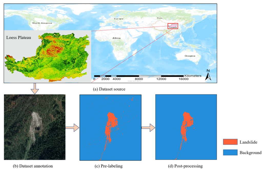
The dataset of images of landslides in this paper are derived from high-resolution remote sensing images and landslide datasets based on terrain interpretation. The contents of the images mainly cover the landslide area of the Loess Plateau.

2.2. Dataset Annotation

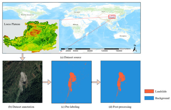
The landslide dataset used in this paper only contains 500 remote sensing images. There are no pixel-level annotations for the landslide areas in these images. Our annotation process, shown in Figure 1, can be divided into three steps: Pre-labeling, Post-processing, Manual correction.

Figure 1. The source and production process of the landslide dataset.

2.2.1. Pre-Labeling

We used support vector machine [15] (SVM) to complete the pre-annotation of the image. SVM is a machine learning algorithm that uses supervised learning methods for the binary classification of data. The learning strategy of SVM is to maximize the interval, which can transform the algorithm process into solving the convex optimal quadratic programming problem. It does not need to rely on overall data, but solves small sample machine learning problems well.

Our specific approach was as follows. On the landslide dataset, for each image, we first manually selected some small rectangular areas that can represent the landslide in the image, then selected some small rectangular areas that represented the background in the picture. It means that, except for the landslide area, other areas are regarded as the background. These areas are support vectors to update the model parameters of the optimized support vector machine to complete the pre-labeling of the landslide dataset.

2.2.2. Post-Processing

We used principal or second components analysis [16] to post-process the labeled images. Principal components analysis (PCA) is a method of post-processing similar to convolution filtering. It classifies all pixels in the region according to which area corresponds to the transform kernel size into principal category. Similarly, second components analysis (SCA) classifies all pixels in the region according to which area corresponds to the transform kernel size into principal category. The formula is as follows:

$$C_{x,y}=F(x,y)=\left\{\begin{array}{cc}\hfill C_{pri},& \hfill (x,y)\in R,PCA,\\ \hfill C_{sec},& \hfill (x,y)\in R,SCA.\end{array}\right.$$

(1)

where R represents the image area of the same size as the transform kernel, $(x,y)$ represents the coordinate position of the pixel, F represents the transform kernel algorithm, $C_{pri}$ represents principal components, $C_{sec}$ represents second components, $C_{x,y}$ represents the category in which the image area is classified.

2.2.3. Manual Correction

Labels obtained through support vector machines and image post-processing methods had several label errors. For this part, we manually corrected this part to obtain the final labeled landslide dataset. With the use of machine learning methods for pre-labeling, manual correction only requires very little human and financial resources compared to manual labeling.

2.3. Dataset Preprocessing

The image sizes in our landslide dataset were different. There were too many pixels in a single remote sensing landslide image. In order to facilitate model training, we cropped the remote sensing image to make it reach a fixed size. At the same time, deep neural networks often require large amounts of data to train to avoid overfitting. To solve this problem, we used data augmentation to increase the diversity of the landslide dataset to better train neural network models.

2.3.1. Image Cropping

We crop the image to a fixed size. For the training set, we use the smooth cropping method to crop the remote sensing image and the corresponding annotation data to a size of $256\times 256$. For the problem of boundary continuity, the overlap ratio was set to $0.25$ during the cropping process. In order to ensure that the number of foreground pixels and background pixels does not differ much, we remove the landslide image where the ratio of landslide pixels is too large or small and only keep the landslide image with the ratio of landslide pixels in the range of 0.05–0.9. For the test set, since the test process does not modify the model weights, the image cropping operation can be omitted.

2.3.2. Data Augmentation

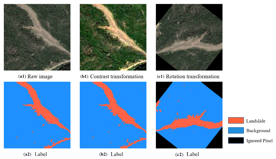
The data augmentation method [17] for image semantic segmentation is similar to other computer vision tasks. The methods we used are mainly as follows:

• Flip transformation;
• Color dithering;
• Contrast transformation;
• Noise perturbation;
• Rotation transformation.

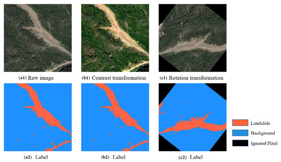
For color dithering, contrast transformation and noise perturbation, the label corresponding to the remote sensing image does not change. For flip transformation and rotation transformation, the label changes as the image changes. It can be seen in Figure 2 that the raw image has some changes in color dithering and rotation transformation.

Figure 2. Data-augmented visualization results with color dithering and rotation transformation.

3. Related Works

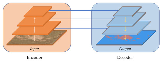
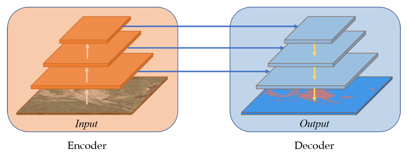
Semantic segmentation [18] is a classic visual scene problem, where the vision task is to take raw image data as input and transform them into masks with salient interests. According to the object, each pixel in the raw image data is assigned to a specified category it belongs to. The semantic segmentation task can provide pixel-level image understanding in a completely human-perceived way. It combines visual tasks such as image classification and object detection. Semantic segmentation divides the image into regional blocks with certain semantic meaning by a specific method and identifies the semantic category of each regional block. It implements the process of the inference from low-level semantics to high-level semantics and finally obtains segmented images with pixel-by-pixel annotations. At present, image semantic segmentation methods include traditional machine learning methods [19] and modern deep learning methods [20]. Traditional semantic segmentation methods can be divided into statistical-based methods [21] and geometric-based methods [22]. With the continuous development of artificial intelligence, the semantic segmentation method of deep learning greatly surpasses the traditional semantic segmentation method. Compared with traditional semantic segmentation methods, deep learning methods use neural networks to automatically learn image features and directly complete end-to-end learning tasks. A large quantity of image semantic segmentation experiments showed that deep learning methods perform better in improving the accuracy of semantic segmentation. The current mainstream end-to-end semantic segmentation networks based on deep learning are encoder-decoder structures, which is shown in Figure 3. The encoder extracts the features of the original image, and the decoder completes the fusion of information based on these features, thereby completing the pixel-by-pixel prediction of the original image.

Figure 3. The encoder-decoder architecture.

3.1. Mainstream Encoder Networks

3.1.1. Convolutional Neural Network

Convolutional neural network [23] is a kind of feedforward neural network [24] including convolutional computation, and has the ability of representation learning. While ensuring translation invariance, convolutional neural network can process input data according to its hierarchical structure. The structural characteristics of convolutional neural networks are local area connection, weight sharing, and downsampling. These characteristics effectively reduce the number of parameters of the network and alleviate the overfitting problem of the model. The main structure of the convolutional neural network is as follows:

• Convolutional layer
  Each convolutional layer consists of several convolution kernels. The parameters of each convolution are obtained through the back-propagation algorithm. The purpose of the convolution operation is to extract different features of the input data. Shallow convolution can extract low-level features such as edges, lines, and corners. Deep convolution can extract more complex high-level features.
• Rectified Linear Units layer
  This layer needs to use an activation function [25]. The activation function activates a certain part of the neurons in the neural network and transmits the activation information to the next layer of the neural network. Activation functions are generally non-linear functions. The reason why neural networks can solve non-linear problems is that they introduce a non-linear activation function which makes up for the expressive ability of the linear model.
• Pooling layer
  After the convolutional layer, features with larger dimensions will be obtained. The pooling operation can divide the features into several regions. Then, it performs some operations, such as taking maximum value or average value, to obtain new, smaller dimensional features. The pooling operation [26] can achieve a nonlinear effect and expand the receptive field. The pooling operation also has the invariance of translation, rotation and scale.
• Fully-Connected layer
  The function of this layer is to integrate the semantic information output by each block, which combines local information into global information to calculate the final classification score. When the convolutional neural network is used as an encoder, the fully connected layer [27] will be removed.

At present, there are various variants of convolutional neural networks. Representative networks include VGGNet [28], ResNet [29], ConvNeXt [30], etc. Lightweight convolutional networks [31] include ShuffleNet [32], MobileNet [33], EfficientNet [34], etc.

3.1.2. Transformer Architecture

Before the advent of Transformer [11], the mainstream networks in natural language processing [35] were based on recurrent or convolutional neural networks. The recurrent neural network [36] connected by the attention mechanism has the best performance. Recurrent neural network is a sequential model [37] which cannot solve the problem of long dependencies [38]. When the sequence of input data is too long, in the process of data processing by the sequence model, the information will be gradually lost. At the same time, it is also difficult to perform parallel computing in the sequential model. Transformer is a simple model that abandons the neural network structure of recurrent and convolution and only relies on the attention mechanism. Transformer introduces a self-attention mechanism that makes the modeling of dependencies independent of the input and output sequences, which solves the problem of long-distance dependencies and supports parallel computing.

By the end of 2020, Transformer had shown a revolutionary improvement in the field of computer vision. Transformer architecture surpassed the performance of the convolutional neural network, which often topped the vision list in many fields. This also showed that computer vision and natural language processing were expected to be unified under the Transformer [13] architecture. The power of the Transformer network relies on the self-attention mechanism. Its main structure mainly includes:

• Self-attention
  The attention mechanism formula is as follows:

  $$Attention(Q,K,V)=Softmax\left(\frac{Q{K}^T}{\sqrt{d_k}}\right)$$

  (2)

  where the matrix Q, K, V has the same dimensions $N\times C$, $N=H\times W$, which represent the length of the sequence, C represents the embedding dimensions, where $\frac{1}{\sqrt{d_k}}$ is the scaling factor.

  $$Q,K,V=Linear\left(X\right),Linear\left(X\right),Linear\left(X\right)$$

  (3)

  where X represents the input features. Self-attention does linear mapping based on the attention mechanism to obtain the matrix $Q,K,V$.

  $$\begin{array}{c}\hfill MultiHead(Q,K,V)=Linear\left(Concat(hea{d}_1,hea{d}_2,...,hea{d}_n)\right)\\ \hfill wherehea{d}_i=Attention(Q_i,K_i,V_i)\end{array}$$

  (4)

  where $Q,K,V$ is split into Multi-Head $Q_{1,2,...,n},K_{1,2,...,n},V_{1,2,...,n}$. By calculating the attention of multiple heads, it will be found that each of the different channels in the space of attention is different. While the computational complexity of the model is similar, the representation ability of the model is improved.
• Positional Encodings
  Since Transformer contains no recurrence and no convolution, in order for Transformer to make use of the order of the sequence, Transformer is injected with some information about the relative or absolute position of the tokens in the sequence. The positional encodings have the same dimension as the embeddings. There are many choices of positional encodings [39]. However, Transformer uses sine and cosine functions of different frequencies:

  $$\begin{array}{c}\hfill P{E}_{pos,2i}=sin(pos/{10000}^{2i/d_{model}})\\ \hfill P{E}_{pos,2i+1}=cos(pos/{10000}^{2i/d_{model}})\end{array}$$

  (5)

  where pos is the position, i is the dimension and $d_{model}$ is the embedding dimensions. That is, each dimension of the positional encoding corresponds to a sinusoid.

At present, there are applications based on transformers in three major visual fields of classification, detection and segmentation. Representative networks include ViT [40], Mix Transformer [41], Swin Transformer [42], etc.

3.2. Mainstream Decoder Networks

3.2.1. Symmetrical Architecture

Symmetric network [43] can actually be regarded as a codec structure. Representative networks include UNet [44] and LinkNet [45], etc. UNet is a U-shaped symmetric structure with convolutional layers on the left and upsampling layers on the right. When implementing, we can design the network from scratch and initialize the weights. After that, we train the model, also can use the existing network and load the corresponding trained weight files, then we build the upsampling layers for training calculation. Lineknet draws on the idea of U-Net, and the innovation of it lies in the connection between the encoder and the decoder. After multiple downsampling by the encoder, spatial information is lost partly. It is difficult to restore the lost spatial information in the decoder part, so the input and output of the encoder are sent together to the network for training.

3.2.2. Multi-Scale Analysis

Multi-scale analysis is a representative method in image processing which has been widely used in various neural networks. The specific method is to use the inherent multi-scale pyramid hierarchy of deep convolutional neural networks to construct feature pyramids with marginal additional cost. Currently, there are many variants of feature pyramid networks [46], such as the Pyramid Scene Parsing Network [47] (PSPNet). It is a multi-scale network that can better learn global contextual representations of scenes. PSPNet uses a residual network as a feature extractor to extract different feature maps. Then, according to different size patterns, these features are mapped into the pyramid module. Each scale-sized feature map corresponds to a pyramid layer. At the same time, these feature maps are processed to reduce the dimensions by a 1 × 1 convolutional layer. The output of the pyramid is upsampled and concatenated with the initial feature maps to capture local and global contextual information. Finally, pixel-wise prediction is finished by using a softmax layer.

3.2.3. DeepLab Based on Dilated Convolution

Dilated convolution [48] introduces dilated rate in the convolutional layer. It can enlarge the receptive field without increasing the computational cost. The Deeplabv2 [49] network uses dilated convolution to solve the problem of reduced resolution in the network caused by max pooling and striding. The key structure of Deeplabv2 network is Atrous Spatial Pyramid Pooling (ASPP). To classify the center pixel, ASPP exploits multi-scale features by employing multiple parallel filters with different rates. Deeplab-ASPP captures object and image context at multiple scales to reliably segment objects at multiple scales. It combines the methods of deep CNN networks and probabilistic graphical models to improve the localization of object boundaries. On this basis, Deeplabv3 [50] proposes a more general framework which is suitable for semantic segmentation tasks in more scenarios. The Deeplabv3 model can control feature extraction and learn network structure of multi-scale features. In the Deeplabv3 model, based on the pre-trained ResNet, the last ResNet block uses dilated convolution. At the same time, it uses different hole rates to obtain multi-scale information, and the decoding part also uses Atrous Space Pyramid Pooling.

4. Methods

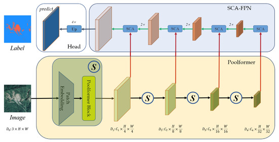
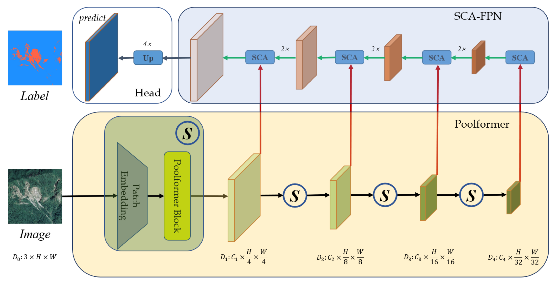
The framework of our Separable Channel Attention Network (SCANet) is based on mainstream Encoder-Decoder architectures, which are illustrated in Figure 4. The framework consists of two parts, Poolformer [51] as the encoder and Separable Channel Attention Feature Pyramid Network (SCA-FPN) as the decoder. Firstly, Poolformer is improved on the basis of Transfromer architecture. Poolformer replaces the self-attention mechanism in Transformer with a pooling operation. This replacement greatly reduces the complexity of the network while maintaining very good performance. Secondly, SCA-FPN is a feature pyramid structure. We inserted a separable channel attention module that we designed originally into SCA-FPN. Separable channel attention includes spatial attention and channel attention. SCA-FPN can fuse different levels of spatial information and channel information obtained by separable channel attention. At the same time, Separable channel attention is an independent module in the calculation process, so that it can be easily embedded and used in other networks. The overall SCANet network, we designed, is spliced by Poolformer and SCA-FPN, and it exhibits better performance with reduced network computational complexity.

Figure 4. The framework of the proposed SCANet, which consists of the Poolformer as encoder, Separable Channel Attention Feature Pyramid Network (SCA-FPN) as decoder. S means Poolformer block.

4.1. Poolformer Encoder

Poolformer adopts the same general framework as Transformer. Its structure is shown in Figure 4. Poolformer has the ability to extract multi-scale information. Given an input image $I\in R^{H\times W\times C}$, we fed it into Poolformer to extract features to obtain multi-level feature maps $C_i(i=1,2,3,4)$ in size $S_i\in$$\left\{\frac{1}{4},\frac{1}{8},\frac{1}{16},\frac{1}{32}\right\}$ of the original image resolution. Poolformer has four important components, including Patch Embedding, Layer Normalization, Residual Connection and Toekn Mixers.

4.1.1. Patch Embedding

The function of Patch Embedding [52] is encoding the input image to adapt the input interface of Poolformer. It cuts an input image into a series of image blocks which have the same size, then encodes the image blocks by convolution to obtain image embedding. Convolution kernel is the same as the size of the image block. In order to ensure the continuity between the image blocks, we use an overlap cutting method in the process of converting the image into image blocks. Another function of Patch Embedding is to downsampling the feature map between Poolformer blocks. It means that each Poolformer block has Patching Embedding. Regardless of continuity, Patch Embedding can be expressed as:

$$\begin{array}{c}\hfill Y_{H_o\times W_o}=Con{v}_{K\times K}\left(X_{H_i\times W_i}\right)\\ \hfill Z_N=InputEmbed\left(Y_{H_o\times W_o}\right)\end{array}$$

(6)

where Y represents the output feature, X represents the input feature, $H_o=\frac{H_i}{k}$, $W_o=\frac{W_i}{k}$, $N=H_o\times W_o$.

4.1.2. Layer Normalization

In the process of using the gradient descent algorithm to optimize model parameters, with the deepening of the network depth, data distribution will have changed. In order to ensure the stability of data distribution and prevent the occurrence of gradient explosion, it is necessary to normalize the data transmitted in the network. Batch Normalization [53] is usually used in convolutional neural networks to normalize data in the dimension of batches. It can balance the data distribution and speed up the convergence of the network. However, for modeling problems of uncertain length sequences, Batch Normalization cannot be embedded in the network to use. Poolformer is actually an indeterminate long sequence modeling network, so it adds Layer Normalization [54] to each Poolformer block rather than Batch Normalization. Layer Normalization prevents gradient diffusion and speeds up parameter convergence for Poolformer. Different from Batch Normalization, Layer Normalization calculates the mean and variance in the channel dimension to normalize the data. The specific formula is as follows:

$$\begin{array}{c}\hfill {\mu }^l=\frac{1}{H}\sum _{i=1}^H{x}_i^l\\ \hfill {\sigma }^l=\sqrt{\frac{1}{H}\sum _{i=1}^H{(x_i^l-{\mu }^l)}^2}\\ \hfill y^l=\frac{x^l-{\mu }^l}{{\sigma }^l+ϵ}\ast \gamma +\beta \end{array}$$

(7)

where l represents the number of layers of the neural network, H represents the number of hidden units in the layer, $ϵ$ is the bias that prevents standard deviation from being zero, $\gamma$ and $\beta$ are linear affine transformation parameters.

4.1.3. Residual Connection

Poolformer is a network with deep layers like Transformer. As the number of neural network layers increases, semantic information at different levels in Poolformer can be extracted. After obtaining a large amount of shallow and deep semantic information, we will have more ways to fuse this semantic information to make more accurate predictions. However, too-deep neural network layers will lead to some problems, such as vanishing gradients and exploding gradients. With the number of network layers increasing, the characteristics of the neural network also change unpredictably. The performance of a deep network may be worse than that of a shallow network. Residual structure can solve the problem of network degradation, vanishing gradients and exploding gradients very well. In Poolformer, adjacent layers are connected through a residual structure. Residual connection is defined as the superposition of the input and the nonlinear change of the input. The formula of the residual connection is as follows:

$$x_{l+1}=f(h\left(x_l\right)+F(x_l,W_l))$$

(8)

where l represents the position of the network layer, W represents the weight of the network layer, $h,F,f$ are short-cut mapping, residual mapping, activation mapping.

4.1.4. Token Mixers

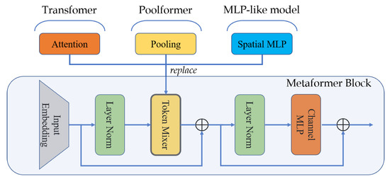
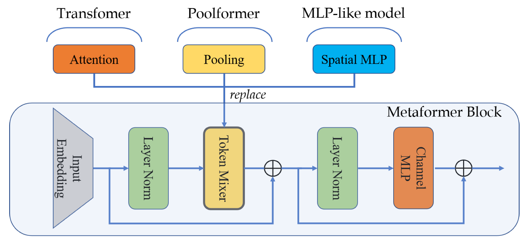
MetaFormer [51]’s components are similar to Transformer except for token mixer. MetaFormer is a general architecture where the token mixer is not specified, which is illustrated in Figure 5. For example, TokenMixer is replaced with a pooling operation in Poolformer. Embedding tokens that come from Patch embedding X are fed to Metaformer blocks. Each Meataformer block consists of two residual sub-blocks. The first sub-blocks use the token mixer to communicate information from embedding tokens. It can be expressed as:

$$Y=TokenMixer\left(LN\right(X\left)\right)+X$$

(9)

where $LN(·)$ represents Layer Normalization. $TokenMixer(·)$ represents a module that can work for mixing token information such as the self-attention mechanism in vision Transformer models, spatial MLP in MLP-like models [55] and the pooling operation in Poolformer.

Figure 5. Metaformer block. Replace TokenMixer with attention to obtain Transformer block. Replace TokenMixer with pooling to obtain Poolformer block. Replace TokenMixer with spatial MLP to obtain MLP-like models block.

The second sub-blocks use two-layer MLP with non-linear activation to communicate information from token mixer. It can be expressed as

$$Z=\sigma \left(LN\left(Y\right)W_1\right)W_2+Y$$

(10)

where $W_1\in R^{C\times C_{hidden}}$ and $W_2\in R^{C_{hidden}\times C}$ are linear affine transformation parameters. $\sigma (·)$ represents a non-linear activation, such as ReLU, GELU, SiLU.

Compared with Transformer, Poolformer removes Transformer’s self-attention mechanism. The main difference made by Poolformer is using simple pooling as a token mixer. For input data $T\in R^{(C\times W\times H)}$, the pooling operation is expressed as

$$T_{i,j}^{\prime }=\frac{1}{K\times K}\sum _{p,q=1}^K{T}_{i+p-\frac{K+1}{2},j+q-\frac{K+1}{2}}-T_{i,j}$$

(11)

where K is the pooling size.

4.2. SCA-FPN

SCA-FPN is the decoder of SCANet we designed. The function of SCA-FPN is to fuse semantic features of different levels obtained by Poolformer encoder to complete the pixel-level prediction of the original image. SCA-FPN has two important components, including Separable Channel Attention and Feature Pyramid Network.

4.2.1. Separable Channel Attention

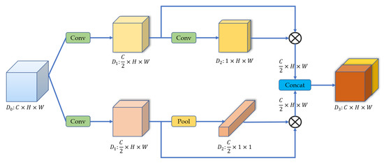
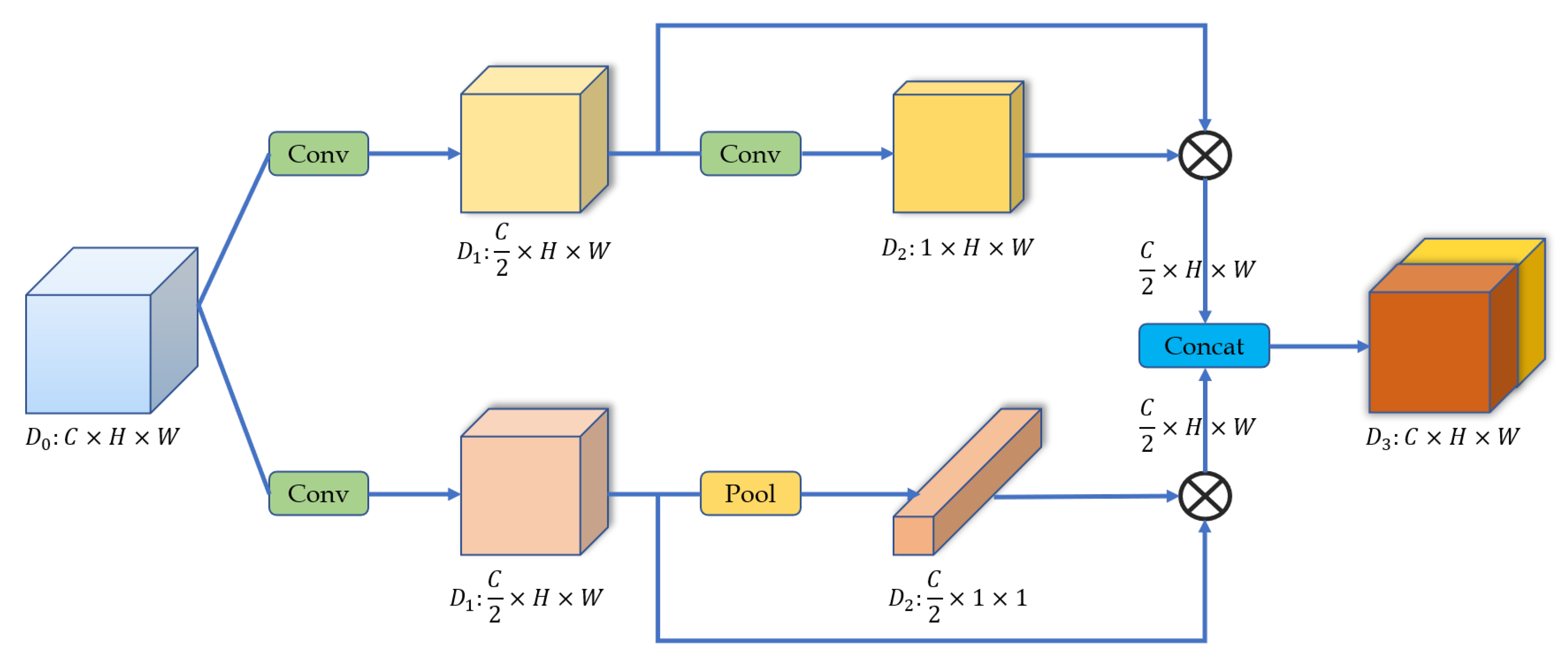
The thought of Separable Channel Attention (SCA) is to focus on different information in different dimensions. Separable channel attention module, shown in Figure 6, divides semantic features into spatial dimensions and channel dimensions. Half of the semantic features are used to focus on spatial information, and half of the semantic features are used to focus on channel information. We use the full convolution operation to get spatial information and use convolution and pooling operations to get channel information. The final feature map is obtained by splicing spatial information and channel information. The specific implementation formula is as follows:

$$\begin{array}{c}\hfill Y_1^s=Con{v}_{\frac{C}{2}\times W\times H}\left(X\right),Y_1^c=Con{v}_{\frac{C}{2}\times W\times H}\left(X\right)\\ \hfill Y_2^s=Con{v}_{1\times W\times H}\left(Y_1^s\right),Y_2^c=Poo{l}_{W\times H}\left(Y_1^c\right)\\ \hfill Z=Concat(Y_1^s\times Y_2^s,Y_1^c\times Y_2^c)+X\end{array}$$

(12)

where $s,c$ represent spatial information and channel information, respectively.

Figure 6. Separable Channel Attention Module.

4.2.2. Feature Pyramid Network

Feature Pyramid Network [46] (FPN) is a structure based on multi-scale analysis. The overall structure of SCA-FPN is a feature pyramid network, which is shown in Figure 4, to fuse low-resolution and high-resolution features. Feature Pyramid Network consists of bottom-up paths, top-down paths and lateral connections.

The bottom-up process is a normal forward propagation process of the neural network. The feature map usually becomes smaller and smaller after being calculated by the convolution kernel. The top-down process is used to upsample more abstract and semantically stronger high-level feature maps. Lateral connection is to merge feature maps obtained in the process of bottom-up and top-dowm. Firstly, we double upsample the low-resolution feature map, and the sampling method is nearest neighbor upsampling. Secondly, we merge the upsampled map with the corresponding bottom-up map by element-wise addition. The overall process is an iterative algorithm.

In our designed SCA-FPN decoder, The fusion method of feature maps is no longer a simple lateral connection. We inserted a SCA module in the laterally connected part of the network to produce the output of each stage. For semantic segmentation task, it uses a two-layer multilayer perceptron at the end of the network to generate masks. Finally, it generates predicted results by the way of upsampling.

4.3. Loss Function

Loss function is used to measure the degree of inconsistency between the predicted value of the model and the real value. In the training phase, our SCANet uses the standard cross-entropy loss and Dice loss [56] as the loss function. For the final predicted output F and the ground truth G, the formula is as follows:

Cross-Entropy Loss

$$loss(F,G)=-\frac{1}{N}\sum _{k=1}^N[G_{k}log\left(F_K\right)+(1-G_k)log(1-F_k)]$$

(13)

Dice Loss

$$loss(F,G)=1-\frac{2|F\cap G|}{\left|F\right|+\left|G\right|}$$

(14)

Total Loss

$$loss=0.5los{s}_{ce}+0.5los{s}_{dice}$$

(15)

where k is the index of pixels and N is the number of pixels in F.

5. Experiments and Discussion

In this section, we conduct extensive experiments on the landslide dataset, which was mentioned in Section 2 to evaluate the the performance of our proposed SCANet. The details of the experimental setup are in Section 5.1. The comparison experiments and analysis of SCANet and mainstream semantic segmentation networks on the landslide dataset are provided in Section 5.2. The ablation experimental results and analysis on Poolformer and separable channel attention module are presented in Section 5.3. Overall effectiveness analysis of SCANet and mainstream semantic segmentation networks is provided in Section 5.4.

5.1. Experimental Settings

5.1.1. Implementation Details

We divide the landslide dataset into a training set and a test set. Due to the small number of data sets, the test set and validation set are the same. In the process of training the model, we perform data augmentation operations on the training set. The specific implementation is is shown in Table 1.

Table 1. The specification of the landslide remote sensing images dataset.

Landslide Dataset	Number	Size	Augmentation
Training Set	1802	256 × 256	√
Validation/Test Set	591	256 × 256	-

The SCANet is implemented in the PyTorch framework, trained and tested on a platform with a single NVIDIA GeForce RTX 3060(12 GB RAM) with CUDA version 10.3 and Cudnn version 8.2.0. On the landslide dataset, we randomly cropped $256\times 256$ patches from the original image and randomly mirrored and rotated them with specified angles ($0^{\circ },{90}^{\circ },{180}^{\circ },{270}^{\circ }$). The stochastic gradient descent with momentum (SGDM) optimizer with a momentum of 0.9 and an initial learning rate of 0.001 was set to guide the optimization. During the network training, a poly learning rate policy was adopted to adjust the learning rate. The batch size was set to 16 and the total number of training epochs was set to 300. Experimental settings are shown in Table 2.

Table 2. Experimental settings.

Configuration	Contents
Operating system	Ubuntu 18.04.5 LTS
GPU	NVIDIA GeForce RTX 3060 (12 GB RAM)
Deep-learning framework	Pytorch 1.11.0 and Torchvision 0.12.0
Parallel computer platform	Cuda 11.3 and Cudnn 8.2.0
Program	Python 3.7.11
Optimizer	SGDM
Learning rate	0.001
LR policy	Poly
Batch size	16
Total epochs	300
Momentum	0.9
Data augmentation	Random flip and Random rotate
Loss function	CrossEntropy and Dice

5.1.2. Comparison Methods and Evaluation Metrics

Intending to fully prove the performance of the proposed SCANet for semantic segmentation of landslide remote sensing images, we compare the proposed SCANet with ten mainstream semantic segmentation networks based on Encoder-Decoder architecture, including MobileNetv2-DeepLabv3Plus [50,57], MobileNetv2-UNet [44,57], MobileNetv2-FPN [46,57], MobileNetv2-PSPNet [47,57], MobileNetv2-LinkNet [45,57], ResNet50-DeepLabv3Plus [29,50], ResNet50-UNet [29,44], ResNet50-FPN [29,46], ResNet50-PSPNet [29,47] and ResNet50-LinkNet [29,45].

In order to fairly compare our proposed SCANet with mainstream semantic segmentation methods on the landslide dataset, we use the widely used evaluation metrics as follows:

IoU

$$\begin{array}{c}\hfill Io{U}_i=\frac{x_{i,i}}{{\sum }_{j=1}^n{x}_{i,j}+{\sum }_{j=1}^n{x}_{j,i}-x_{i,i}}\\ \hfill mIoU=\frac{1}{n}\sum _{i=1}^{n}Io{U}_i\end{array}$$

(16)

where $x_{i,j}$ means the number of instances of class i predicted as class j, and n is the number of classes.

Accuracy

$$OA=\frac{TP+TN}{P+N}$$

(17)

where $OA$ is the ratio of the number of correctly predicted pixels to the total number of pixels.

F1-score

$$F_1=2\times \frac{precision\times recall}{precision+recall}$$

(18)

where $precision=\frac{TP}{TP+FP}$ and $recall=\frac{TP}{TP+FN}$.

5.2. Comparative Experiments

We follow the experimental setup in Section 5.1 and conduct extensive experiments on the landslide dataset to compare the performance of our proposed SCANet and mainstream semantic segmentation networks, including MobileNetv2-DeepLabv3Plus [50,57], MobileNetv2-UNet [44,57], MobileNetv2-FPN [46,57], MobileNetv2-PSPNet [47,57], MobileNetv2-LinkNet [45,57], ResNet50-DeepLabv3Plus [29,50], ResNet50-UNet [29,44], ResNet50-FPN [29,46], ResNet50-PSPNet [29,47] and ResNet50-LinkNet [29,45].

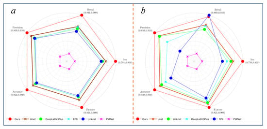
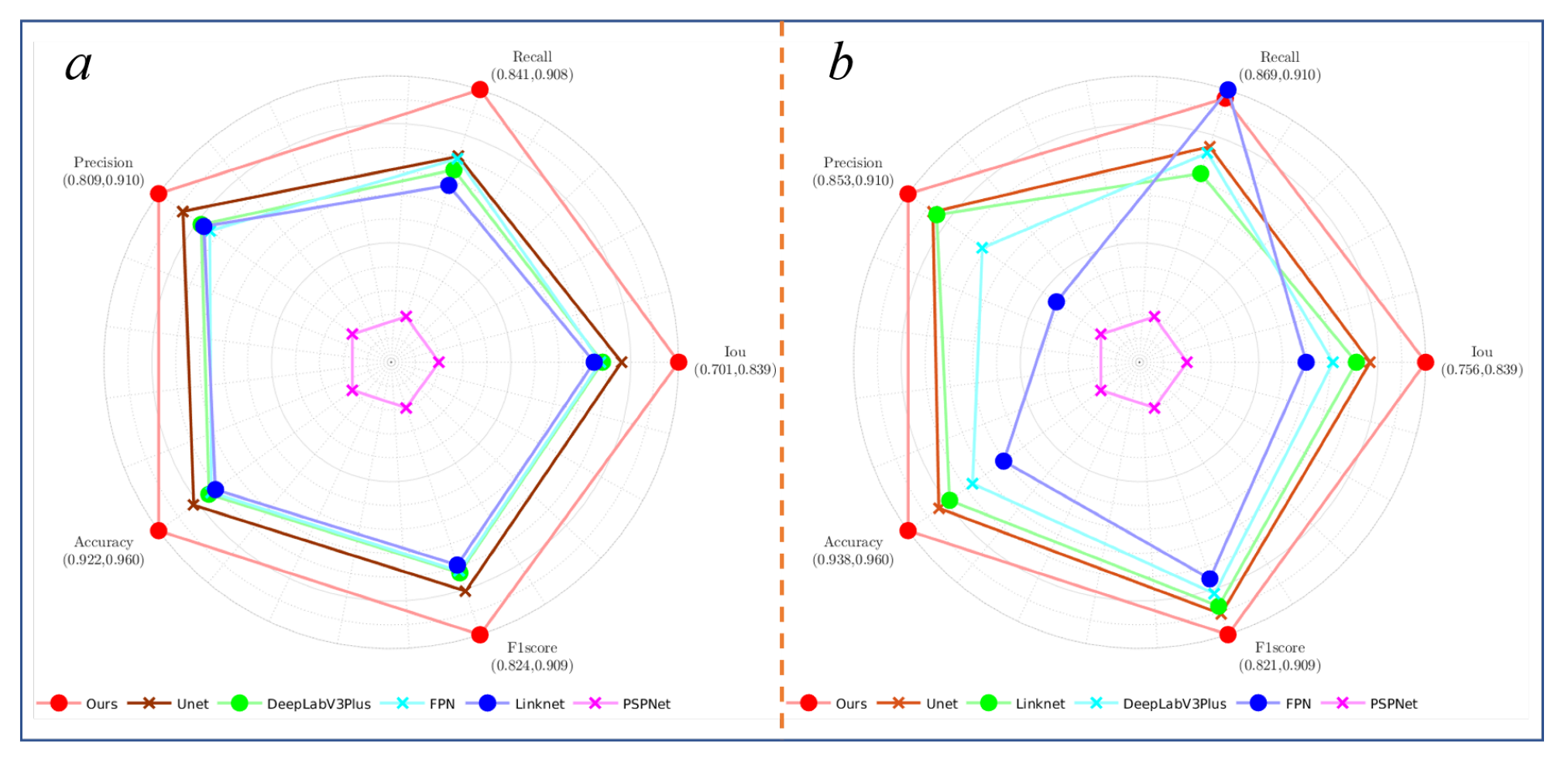
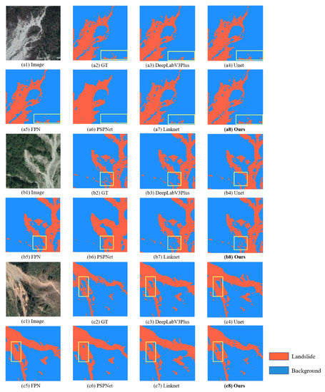
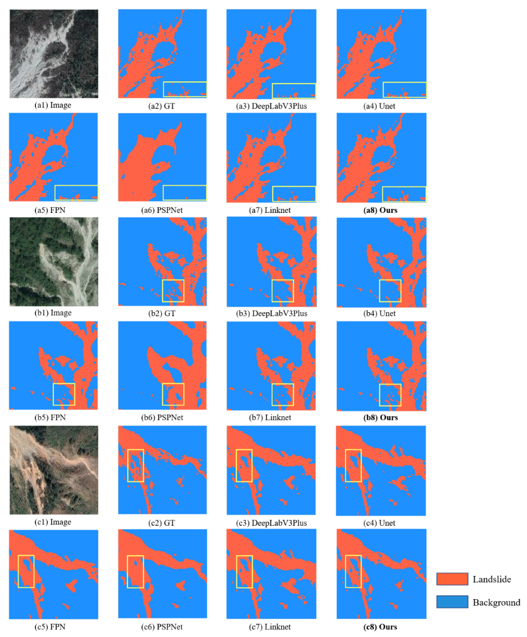
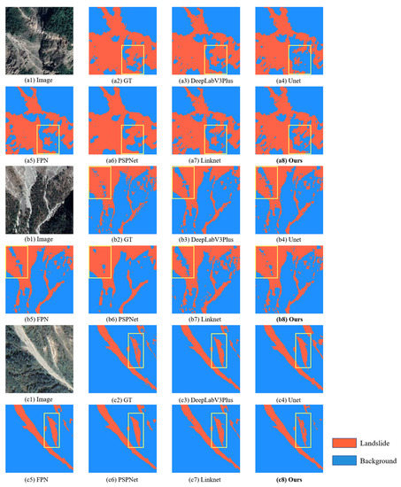
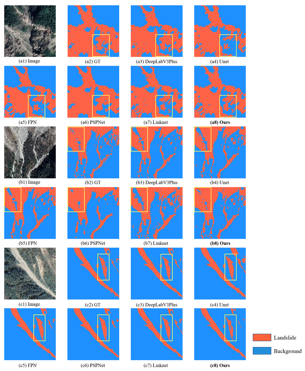
The quantitative results of our comparative experiments on the landslide dataset are shown in Table 3. The visual analysis of evaluation metrics is shown in Figure 7, the visualization results of our proposed SCANet and mainstream semantic segmentation networks using Mobilenet_v2 as encoder are shown in Figure 8 and the visualization results of our proposed SCANet and mainstream semantic segmentation networks using ResNet50 as encoder are shown in Figure 9. Our proposed SCANet achieve SOTA in all semantic segmentation methods mentioned above.

Table 3. The quantitative results of mainstream semantic segmentation methods and the proposed SCANet. The best results are highlighted in bold, and the second-best results are underlined.

Method		Recall (%)	Precision (%)	OA (%)	F1-score (%)	IoU (%)	Params (M)	Times (ms/Img)
Encoder	Decoder
Mobilenet_v2	DeepLabV3Plus	88.45	88.76	95.02	88.60	79.54	4.4	9.388
Mobilenet_v2	Unet	88.85	89.71	95.32	89.28	80.64	6.6	8.217
Mobilenet_v2	FPN	88.78	88.31	94.97	88.54	79.44	4.2	8.243
Mobilenet_v2	PSPNet	84.09	80.86	92.16	82.44	70.13	2.3	7.245
Mobilenet_v2	Linknet	87.99	88.62	94.89	88.31	79.06	4.3	7.837
ResNet50	DeepLabV3Plus	89.84	88.77	95.29	89.31	80.68	26.7	11.699
ResNet50	Unet	89.96	90.24	95.67	90.10	81.98	32.5	11.955
ResNet50	FPN	90.98	86.58	94.94	88.73	79.74	26.1	10.773
ResNet50	PSPNet	86.91	85.26	93.84	82.05	75.57	24.3	9.325
ResNet50	Linknet	89.48	90.13	95.55	89.80	81.50	31.2	12.624
Poolformer	SCA-FPN	90.83	90.98	96.02	90.91	83.93	21.6	11.426

Figure 7. Visual analysis of evaluation metrics. (a) Visualization of the proposed SCANet compared with other networks (MobileNetv2-DeepLabv3Plus, MobileNetv2-UNet, MobileNetv2-FPN, MobileNetv2-PSPNet and MobileNetv2-LinkNet) using Mobilenet_v2 as encoder; (b) Visualization of the proposed SCANet compared with other networks (ResNet50-DeepLabv3Plus, ResNet50-UNet, ResNet50-FPN, ResNet50-PSPNet and ResNet50-LinkNet) using ResNet50 as encoder.

Figure 8. The visualization results of our proposed SCANet and mainstream semantic segmentation networks (MobileNetv2-DeepLabv3Plus, MobileNetv2-UNet, MobileNetv2-FPN, MobileNetv2-PSPNet and MobileNetv2-LinkNet) using Mobilenet_v2 as encoder.

Figure 9. The visualization results of our proposed SCANet and mainstream semantic segmentation networks (ResNet50-DeepLabv3Plus, ResNet50-UNet, ResNet50-FPN, ResNet50-PSPNet and ResNet50-LinkNet) using ResNet50 as encoder.

As can be observed from Table 3 and Figure 7, our method achieves the best results on the evaluation metrics of Precision, OA, F1-score and IoU. Compared with mainstream semantic segmentation networks that use Mobilenet_v2 [57] as an encoder, though the amount of our model parameters increased, our method performed well. Specifically, our proposed SCANet outperformed the second-best method, Mobilenet_v2-Unet [44,57], by 3.29% and the third-best method, Mobilenet_v2-DeepLabV3Plus [50,57], by 4.39% in the IoU score. Compared with mainstream semantic segmentation networks that use ResNet50 [29] as an encoder, our method performed well while the amount of our model parameters decreased. Specifically, our proposed SCANet outperformed the second-best method, ResNet50-Unet [29,44], by 1.95% and the third-best method, ResNet50-DeepLabV3Plus [29,50], by 3.25% in the IoU score.

In addition, we conduct many detailed visual comparison experiments, further confirming the performance of the proposed SCANet for semantic segmentation tasks on the landslide dataset. The visualization results of the proposed SCANet and mainstream semantic segmentation networks that use Mobilenet_v2 [57] as an encoder are shown in Figure 8. The visualization results of the proposed SCANet and mainstream semantic segmentation networks that use ResNet50 [29] as an encoder are shown in Figure 9. Benefitting from Poolformer encoder, which effectively transfers global information to each pyramid-level feature map, SCANet can generate high-resolution feature maps with high-level semantic information. Benefitting from SCA-FPN decoder, which introduced separable channel attention, SCANet can predict the edge texture information of the image more accurately. The combination of Poolformer encoder and SCA-FPN decoder makes our method achieve the best performance.

5.3. Ablation Experiments

In this subsection, we evaluate the effectiveness of two key modules of our proposed SCANet based on Encoder-Decoder architecture, Poolformer as the encoder module, Separable Channel Attention used in SCA-FPN. The ablation experiments are also trained and tested on the landslide dataset. To verify the effect of Poolformer encoder, we conduct extensive ablation experiments in Section 5.3.1 that compare Poolformer with ResNet50 while keeping the decoder consistent. To verify the effect of Separable Channel Attention, we conduct extensive ablation experiments in Section 5.3.2 that compared SCA-FPN with FPN while keeping the encoder consistent.

5.3.1. Effect of Poolformer

Poolformer encoder can be spliced with many decoding modules flexibly, such as Unet [44], FPN [46], PSPNet [47], LinkNet [45]. Poolformer encoder was used to obtain pyramid-level features, and the final output was expressed as:

$$Out=Up(Up(Up(Up\left(C_1\right)+C_2)+C_3)+C_4)$$

(19)

where $C_i(i=1,2,3,4)$ represents pyramid-level features, $Up$ represents upsampling.

As can be seen in Table 4, semantic segmentation networks using Poolformer encoder had better effects than networks using ResNet50 encoder, improving the IoU by 2.79%, 1.97%, 0.73%, 1.24% 2.91%, the F1-score by 1.66%, 1.21%, 0.82%, 0.76% 2.02% while using Unet [44], FPN [46], PSPNet [47], LinkNet [45], SCA-FPN as decoders, respectively. The performance improvement is due to Poolformer encoder, which can capture global information well. Compared with other decoders, the method using SCA-FPN decoder has the largest performance increase, improving the IoU by 2.79%, the F1-score by 1.66% after replacing ResNet50 with Poolformer. It indicates that the SCA-FPN decoder that we designed is more suitable for Poolformer encoder. All in all, Poolformer encoder actually provides a significant performance improvement for landslide scene segmentation.

Table 4. The quantitative results of different semantic segmentation networks using ResNet50 and Poolformer as encoders, respectively. The results of semantic segmentation network using Poolformer as encoder are highlighted in bold.

Decoder	Encoder		IoU (%)	F1-score (%)
	ResNet50	Poolformer
Unet	√	-	81.98	90.10
	-	√	84.77	91.76
FPN	√	-	79.74	88.73
	-	√	81.71	89.94
PSPNet	√	-	75.57	82.05
	-	√	76.30	82.87
Linknet	√	-	81.50	89.80
	-	√	82.74	90.56
SCA-FPN	√	-	81.02	88.89
	-	√	83.93	90.91

5.3.2. Effect of SCA

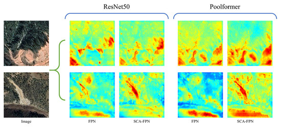
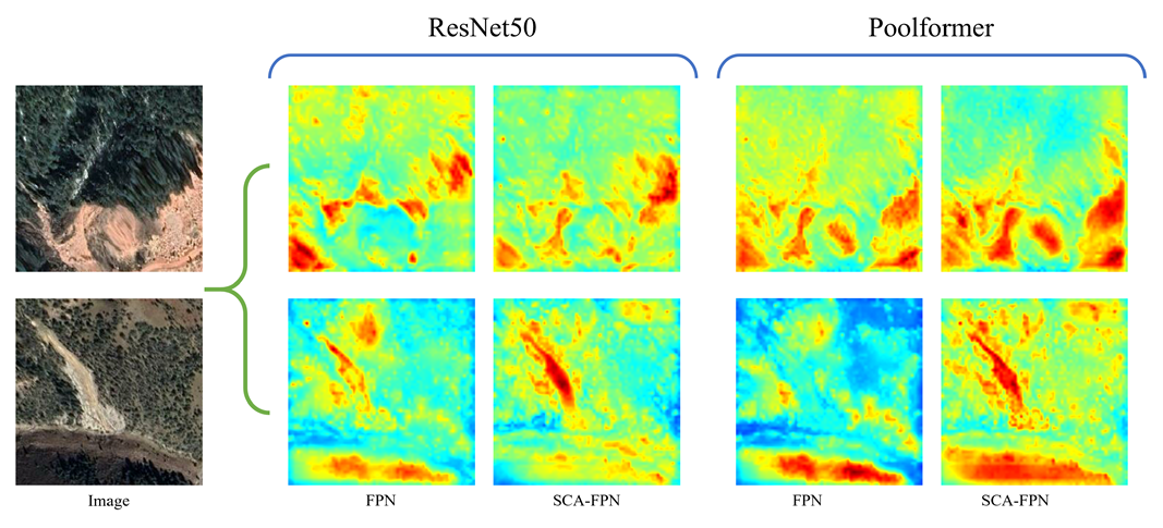
We evaluate the effectiveness of our proposed SCA module by comparing FPN with SCA-FPN while keeping the encoder consistent. As is shown Table 5, the landslide segmentation performance is improved after adding SCA. ResNet50-SCA-FPN improves the IoU score by 1.28% compared to ResNet50-FPN while both networks use ResNet50 encoder. SCANet improves the IoU score by 2.22% compared to Poolformer-FPN while both networks use Poolformer encoder. Figure 10 shows four models’ heatmap that derived from the features before the network classification layer. We can see the network’s attention to the landslide area is enhanced after replacing FPN with SCA-FPN. It indicates the insertion of SCA makes the model pay more attention to the edge region and texture of the landslide area. Therefore, SCA is surely an effective module for semantic segmentation network in the landslide scene.

Table 5. The quantitative results of different semantic segmentation networks using FPN and SCA-FPN as decoders, respectively.

Encoder		Decoder		IoU (%)	F1-score (%)
ResNet50	Poolformer	FPN	SCA-FPN
√	-	√	-	79.74	88.73
√	-	-	√	81.02	88.89
-	√	√	-	81.71	89.94
-	√	-	√	83.93	90.91

Figure 10. The heatmap that derived from the features before the network classification layer on different networks.

5.4. Analysis of Methods

We test the current mainstream semantic segmentation methods in the landslide scene. On our landslide dataset, experiments are carried out to evaluate the performance of each method. Comparing different SOTA networks, the neworks (MobileNetv2-UNet [44,57], ResNet50-UNet [29,44]) using Unet decoder performs the best. Unet decoder, as a representative of a lightweight decoder, achieves the best performance with combinations of different encoders.

Our proposed SCANet uses Poolformer as an encoder and SCA-FPN as a decoder. Unlike convolutional neural networks, Poolformer is based on Transformer architecture. In Poolformer, self-attention mechanisms in the network are replaced by pooling layers, which ensure that the model computational complexity is low. Compared with ResNet50 encoder, Poolformer encoder performs better while the model complexity is reduced. Besides, based on the FPN decoder, we embed our own designed SCA module to build a new SCA-FPN decoder for feature fusion and pixel prediction. From the ablation experiments, we can see that the SCA-FPN decoder we designed is better than the FPN decoder. SCA-FPN introduces a separable channel attention module to make the landslide area more focused. In short, compared with the mainstream semantic segmentation network mentioned above, our proposed SCANet performs best in the task of semantic segmentation of landslide scenes.

6. Conclusions

In this paper, based on the remote sensing images of landslides on the Loess Plateau, we use machine learning methods to construct a dataset of landslide scenes. In order to compare the performance of current mainstream semantic segmentation networks, we do relevant experiments on the landslide dataset for analysis. Unlike convolutional neural networks, we propose a new framework for semantic segmentation of remote sensing images named Separable Channel Attention Network (SCANet), which relies on the transformer architecture. SCANet contains two components, the Poolformer encoder and the SCA-FPN decoder. In the encoder part, for the convolutional neural network, the trained network cannot capture the global mutual information. However, Poolformer, which we use, makes up for the lack of the convolutional neural network. Limited by the high complexity of the self-attention algorithm in Transformer, Poolformer replaces self-attention mechanisms with pooling operations. This change still maintains network performance better than the convolutional neural network. In the decoder part, in order to make the network pay more attention to the image edge texture information, SCA-FPN uses a feature pyramid structure to obtain multi-scale information. The separable channel attention mechanism we designed is also inserted into SCA-FPN, which makes the network pay more attention to the foreground information and improves the accuracy of pixel-level classification.

In addition, we conduct extensive experiments on the landslide dataset. Through these experiments, we demonstrate that our SCANet can achieve good segmentation results on the semantic segmentation task of the remote sensing images. Our network outperforms other mainstream methods on the landslide dataset. Our research also validates that semantic segmentation techniques can be used to locate and estimate landslide areas. We hope this research can inspire more researchers in this area and deploy practical applications.

References

- Davies, T. Landslide hazards, risks, and disasters: Introduction. In Landslide Hazards, Risks, and Disasters; Elsevier: Amsterdam, The Netherlands, 2015; pp. 1–16. [Google Scholar]
- Baum, R.L.; Godt, J.W.; Savage, W.Z. Estimating the timing and location of shallow rainfall-induced landslides using a model for transient, unsaturated infiltration. J. Geophys. Res. Earth Surf. 2010, 115, F03013. [Google Scholar] [CrossRef] [Scilit]
- Camps-Valls, G.; Tuia, D.; Gómez-Chova, L.; Jiménez, S.; Malo, J. Remote sensing image processing. Synth. Lect. Image Video Multimed. Process. 2011, 5, 1–192. [Google Scholar]
- LeCun, Y.; Bengio, Y.; Hinton, G. Deep learning. Nature 2015, 521, 436–444. [Google Scholar] [CrossRef] [Scilit]
- Dey, V.; Zhang, Y.; Zhong, M. A Review on Image Segmentation Techniques with Remote Sensing Perspective; ISPRS IC VII Symposium: Vienna, Austria, 2010; Volume 38. [Google Scholar]
- Liu, D.; Li, Y.; Lin, J.; Li, H.; Wu, F. Deep learning-based video coding: A review and a case study. ACM Comput. Surv. (CSUR) 2020, 53, 1–35. [Google Scholar] [CrossRef] [Scilit]
- Voulodimos, A.; Doulamis, N.; Doulamis, A.; Protopapadakis, E. Deep learning for computer vision: A brief review. Comput. Intell. Neurosci. 2018, 2018, 7068349. [Google Scholar] [CrossRef] [Scilit]
- Ghorbanzadeh, O.; Blaschke, T.; Gholamnia, K.; Meena, S.R.; Tiede, D.; Aryal, J. Evaluation of different machine learning methods and deep-learning convolutional neural networks for landslide detection. Remote Sens. 2019, 11, 196. [Google Scholar] [CrossRef] [Scilit]
- Badrinarayanan, V.; Kendall, A.; Cipolla, R. Segnet: A deep convolutional encoder-decoder architecture for image segmentation. IEEE Trans. Pattern Anal. Mach. Intell. 2017, 39, 2481–2495. [Google Scholar] [CrossRef] [Scilit] [PubMed]
- Albawi, S.; Mohammed, T.A.; Al-Zawi, S. Understanding of a convolutional neural network. In Proceedings of the 2017 International Conference on Engineering and Technology (ICET), Antalya, Turkey, 21–23 August 2017; pp. 1–6. [Google Scholar]
- Vaswani, A.; Shazeer, N.; Parmar, N.; Uszkoreit, J.; Jones, L.; Gomez, A.N.; Kaiser, Ł.; Polosukhin, I. Attention is all you need. Adv. Neural Inf. Process. Syst. 2017, 30. [Google Scholar] [CrossRef] [Scilit]
- Niu, Z.; Zhong, G.; Yu, H. A review on the attention mechanism of deep learning. Neurocomputing 2021, 452, 48–62. [Google Scholar] [CrossRef] [Scilit]
- Han, K.; Wang, Y.; Chen, H.; Chen, X.; Guo, J.; Liu, Z.; Tang, Y.; Xiao, A.; Xu, C.; Xu, Y.; et al. A survey on visual transformer. arXiv 2020, arXiv:2012.12556. [Google Scholar]
- Zhang, Z.; Zhang, X.; Peng, C.; Xue, X.; Sun, J. Exfuse: Enhancing feature fusion for semantic segmentation. In Proceedings of the European conference on computer vision (ECCV), Munich, Germany, 8–14 September 2018; pp. 269–284. [Google Scholar]
- Hearst, M.A.; Dumais, S.T.; Osuna, E.; Platt, J.; Scholkopf, B. Support vector machines. IEEE Intell. Syst. Their Appl. 1998, 13, 18–28. [Google Scholar] [CrossRef] [Scilit]
- Dunteman, G.H. Principal Components Analysis; Sage: New York, NY, USA, 1989; p. 69. [Google Scholar]
- Shorten, C.; Khoshgoftaar, T.M. A survey on image data augmentation for deep learning. J. Big Data 2019, 6, 60. [Google Scholar] [CrossRef] [Scilit]
- Lateef, F.; Ruichek, Y. Survey on semantic segmentation using deep learning techniques. Neurocomputing 2019, 338, 321–348. [Google Scholar] [CrossRef] [Scilit]
- Fu, K.S.; Mui, J. A survey on image segmentation. Pattern Recognit. 1981, 13, 3–16. [Google Scholar] [CrossRef] [Scilit]
- Minaee, S.; Boykov, Y.Y.; Porikli, F.; Plaza, A.J.; Kehtarnavaz, N.; Terzopoulos, D. Image segmentation using deep learning: A survey. IEEE Trans. Pattern Anal. Mach. Intell. 2021, 44, 3523–3542. [Google Scholar] [CrossRef] [Scilit]
- Yi, L.; Zhijun, G. A review of segmentation method for MR image. In Proceedings of the 2010 International Conference on Image Analysis and Signal Processing, Zhejiang, China, 9–11 April 2010; pp. 351–357. [Google Scholar]
- Minaee, S.; Fotouhi, M.; Khalaj, B.H. A geometric approach to fully automatic chromosome segmentation. In Proceedings of the 2014 IEEE Signal Processing in Medicine and Biology Symposium (SPMB), Philadelphia, PA, USA, 13 December 2014; pp. 1–6. [Google Scholar]
- O’Shea, K.; Nash, R. An introduction to convolutional neural networks. arXiv 2015, arXiv:1511.08458. [Google Scholar]
- Svozil, D.; Kvasnicka, V.; Pospichal, J. Introduction to multi-layer feed-forward neural networks. Chemom. Intell. Lab. Syst. 1997, 39, 43–62. [Google Scholar] [CrossRef] [Scilit]
- Ramachandran, P.; Zoph, B.; Le, Q.V. Searching for activation functions. arXiv 2017, arXiv:1710.05941. [Google Scholar]
- Sun, M.; Song, Z.; Jiang, X.; Pan, J.; Pang, Y. Learning pooling for convolutional neural network. Neurocomputing 2017, 224, 96–104. [Google Scholar] [CrossRef] [Scilit]
- Basha, S.S.; Dubey, S.R.; Pulabaigari, V.; Mukherjee, S. Impact of fully connected layers on performance of convolutional neural networks for image classification. Neurocomputing 2020, 378, 112–119. [Google Scholar] [CrossRef] [Scilit]
- Muhammad, U.; Wang, W.; Chattha, S.P.; Ali, S. Pre-trained VGGNet architecture for remote-sensing image scene classification. In Proceedings of the 2018 24th International Conference on Pattern Recognition (ICPR), Beijing, China, 20–24 August 2018; pp. 1622–1627. [Google Scholar]
- He, K.; Zhang, X.; Ren, S.; Sun, J. Deep residual learning for image recognition. In Proceedings of the IEEE conference on computer vision and pattern recognition, Las Vegas, NV, USA, 27–30 June 2016; pp. 770–778. [Google Scholar]
- Liu, Z.; Mao, H.; Wu, C.Y.; Feichtenhofer, C.; Darrell, T.; Xie, S. A convnet for the 2020s. In Proceedings of the IEEE/CVF Conference on Computer Vision and Pattern Recognition, New Orleans, LA, USA, 19–20 June 2022; pp. 11976–11986. [Google Scholar]
- Zhou, Y.; Chen, S.; Wang, Y.; Huan, W. Review of research on lightweight convolutional neural networks. In Proceedings of the 2020 IEEE 5th Information Technology and Mechatronics Engineering Conference (ITOEC), Chongqing, China, 12–14 June 2020; pp. 1713–1720. [Google Scholar]
- Zhang, X.; Zhou, X.; Lin, M.; Sun, J. Shufflenet: An extremely efficient convolutional neural network for mobile devices. In Proceedings of the IEEE Conference on Computer Vision and Pattern Recognition, Salt Lake City, UT, USA, 18–22 June 2018; pp. 6848–6856. [Google Scholar]
- Howard, A.G.; Zhu, M.; Chen, B.; Kalenichenko, D.; Wang, W.; Weyand, T.; Andreetto, M.; Adam, H. Mobilenets: Efficient convolutional neural networks for mobile vision applications. arXiv 2017, arXiv:1704.04861. [Google Scholar]
- Tan, M.; Le, Q. Efficientnet: Rethinking model scaling for convolutional neural networks. In Proceedings of the International Conference on Machine Learning, PMLR, Long Beach, CA, USA, 9–15 June 2019; pp. 6105–6114. [Google Scholar]
- Chowdhary, K. Natural language processing. In Fundamentals of Artificial Intelligence; Springer: New Delhi, India, 2020; pp. 603–649. [Google Scholar]
- Mikolov, T.; Karafiát, M.; Burget, L.; Cernockỳ, J.; Khudanpur, S. Recurrent neural network based language model. In Proceedings of the 11th Annual Conference of the International-Speech-Communication-Association 2010, Makuhari, Japen, 1 January 2010; Volume 2, pp. 1045–1048. [Google Scholar]
- Chung, J.; Gulcehre, C.; Cho, K.; Bengio, Y. Empirical evaluation of gated recurrent neural networks on sequence modeling. arXiv 2014, arXiv:1412.3555. [Google Scholar]
- Lin, T.; Horne, B.G.; Tino, P.; Giles, C.L. Learning long-term dependencies in NARX recurrent neural networks. IEEE Trans. Neural Netw. 1996, 7, 1329–1338. [Google Scholar] [PubMed]
- Gehring, J.; Auli, M.; Grangier, D.; Yarats, D.; Dauphin, Y.N. Convolutional sequence to sequence learning. In Proceedings of the International Conference on Machine Learning, PMLR, Sydney, Australia, 6–11 August 2017; pp. 1243–1252. [Google Scholar]
- Dosovitskiy, A.; Beyer, L.; Kolesnikov, A.; Weissenborn, D.; Zhai, X.; Unterthiner, T.; Dehghani, M.; Minderer, M.; Heigold, G.; Gelly, S.; et al. An image is worth 16x16 words: Transformers for image recognition at scale. arXiv 2020, arXiv:2010.11929. [Google Scholar]
- Chen, J.N.; Sun, S.; He, J.; Torr, P.H.; Yuille, A.; Bai, S. Transmix: Attend to mix for vision transformers. In Proceedings of the IEEE/CVF Conference on Computer Vision and Pattern Recognition, New Orleans, LA, USA, 19–20 June 2022; pp. 12135–12144. [Google Scholar]
- Liu, Z.; Lin, Y.; Cao, Y.; Hu, H.; Wei, Y.; Zhang, Z.; Lin, S.; Guo, B. Swin transformer: Hierarchical vision transformer using shifted windows. In Proceedings of the IEEE/CVF International Conference on Computer Vision, Virtual Event, 11–17 October 2021; pp. 10012–10022. [Google Scholar]
- Golubitsky, M.; Stewart, I. Recent advances in symmetric and network dynamics. Chaos Interdiscip. J. Nonlinear Sci. 2015, 25, 097612. [Google Scholar] [CrossRef] [Scilit] [PubMed]
- Ronneberger, O.; Fischer, P.; Brox, T. U-net: Convolutional networks for biomedical image segmentation. In International Conference on Medical Image Computing and Computer-Assisted Intervention; Springer: Berlin/Heidelberg, Germany, 2015; pp. 234–241. [Google Scholar]
- Chaurasia, A.; Culurciello, E. Linknet: Exploiting encoder representations for efficient semantic segmentation. In Proceedings of the 2017 IEEE Visual Communications and Image Processing (VCIP), St. Petersburg, FL, USA, 10–13 December 2017; pp. 1–4. [Google Scholar]
- Lin, T.Y.; Dollár, P.; Girshick, R.; He, K.; Hariharan, B.; Belongie, S. Feature pyramid networks for object detection. In Proceedings of the IEEE Conference on Computer Vision and Pattern Recognition, Honolulu, HI, USA, 21–26 July 2017; pp. 2117–2125. [Google Scholar]
- Zhao, H.; Shi, J.; Qi, X.; Wang, X.; Jia, J. Pyramid scene parsing network. In Proceedings of the IEEE Conference on Computer Vision and Pattern Recognition, Honolulu, HI, USA, 21–26 July 2017; pp. 2881–2890. [Google Scholar]
- Yu, F.; Koltun, V. Multi-scale context aggregation by dilated convolutions. arXiv 2015, arXiv:1511.07122. [Google Scholar]
- Chen, L.C.; Papandreou, G.; Kokkinos, I.; Murphy, K.; Yuille, A.L. Deeplab: Semantic image segmentation with deep convolutional nets, atrous convolution, and fully connected crfs. IEEE Trans. Pattern Anal. Mach. Intell. 2017, 40, 834–848. [Google Scholar] [CrossRef] [Scilit] [PubMed]
- Chen, L.C.; Zhu, Y.; Papandreou, G.; Schroff, F.; Adam, H. Encoder-decoder with atrous separable convolution for semantic image segmentation. In Proceedings of the European conference on computer vision (ECCV), Munich, Germany, 8–14 September 2018; pp. 801–818. [Google Scholar]
- Yu, W.; Luo, M.; Zhou, P.; Si, C.; Zhou, Y.; Wang, X.; Feng, J.; Yan, S. Metaformer is actually what you need for vision. In Proceedings of the IEEE/CVF Conference on Computer Vision and Pattern Recognition, New Orleans, LA, USA, 19–20 June 2022; pp. 10819–10829. [Google Scholar]
- Bailer, C.; Varanasi, K.; Stricker, D. CNN-based patch matching for optical flow with thresholded hinge embedding loss. In Proceedings of the IEEE Conference on Computer Vision and Pattern Recognition, Honolulu, HI, USA, 21–26 July 2017; pp. 3250–3259. [Google Scholar]
- Ioffe, S.; Szegedy, C. Batch normalization: Accelerating deep network training by reducing internal covariate shift. In Proceedings of the International Conference on Machine Learning, PMLR, Lille, France, 7–9 July 2015; pp. 448–456. [Google Scholar]
- Ba, J.L.; Kiros, J.R.; Hinton, G.E. Layer normalization. arXiv 2016, arXiv:1607.06450. [Google Scholar]
- Borji, A.; Lin, S. SplitMixer: Fat Trimmed From MLP-like Models. arXiv 2022, arXiv:2207.10255. [Google Scholar]
- Milletari, F.; Navab, N.; Ahmadi, S.A. V-net: Fully convolutional neural networks for volumetric medical image segmentation. In Proceedings of the 2016 Fourth International Conference on 3D Vision (3DV), Stanford, CA, USA, 25–28 October 2016; pp. 565–571. [Google Scholar]
- Sandler, M.; Howard, A.; Zhu, M.; Zhmoginov, A.; Chen, L.C. Mobilenetv2: Inverted residuals and linear bottlenecks. In Proceedings of the IEEE Conference on Computer Vision and Pattern Recognition, Salt Lake City, UT, USA, 18–23 June 2018; pp. 4510–4520. [Google Scholar]
Publisher’s Note: MDPI stays neutral with regard to jurisdictional claims in published maps and institutional affiliations. |
© 2022 by the authors. Licensee MDPI, Basel, Switzerland. This article is an open access article distributed under the terms and conditions of the Creative Commons Attribution (CC BY) license (https://creativecommons.org/licenses/by/4.0/).