Travel Time Reliability of Highway Network under Multiple Failure Modes

Abstract

Network reliability reflects a system’s ability to perform specified functions under specified topological and traffic conditions. Network reliability is the weighted sum of connection reliability and travel time reliability. Based on complex network theory, a new method was proposed to calculate the travel time reliability of road networks. The topology model of a regional highway network in China was built using the dual method. After a random attack or deliberate attack, node sizes in the sub-network can be used to reflect the node importance for network connection reliability. Some conclusions were drawn after the change in travel time coefficient and delay coefficient. The increases in the two coefficients will accelerate the decrease of travel time reliability of the highway network. After a comparison among three methods of travel time reliability, including variation coefficient, the misery indexes, and the new equation, the new method was further verified. The influence factors of highway network reliability were analyzed under the condition of different highway blockage and congestion.

1. Introduction

Road network reliability (NR) is the reliable degree of road traffic network under a certain service level [1]. Comprehensive evaluation on the reliability of a specific road network can help road managers optimize the road network according to the different traffic flow, improve the overall accessibility of the road network, and put forward a reasonable and feasible emergency plan when traffic accidents or natural disasters occur in parts of the road network. It helps road users to reduce the travel time and improve transportation efficiency.

At present, there are 150,000 km of expressways in China, and the expressways have been connected into a network. The development of a road network has changed from the previous rapid construction stage to the maintenance and operation stage. Therefore, whether the network has a good topology and can operate reliably in the road network needs to be carefully studied.

The structure indexes and operation characters of the road network include invulnerability, reliability, and robustness. The invulnerability of a road transportation system reflects the network sensitivity to traffic incidents, which leads to the decrease of service capacity of the road network [2]. In 1995, a great earthquake occurred in Kobe, Japan. Snelder et al. developed a consistent framework for robustness, including a definition, terms related to robustness, indicators, and an evaluation method [3]. Scholars in the transportation field began to research the reliability of road networks, especially the travel time reliability (TTR) [4]. Road NR is divided into two categories, including connection reliability (CR) and TTR. The former is the system structure index and the latter describes the operation character of the road network. CR describes the connection probability between two network nodes. TTR describes the probability that a trip can be completed within a certain time range. Carrion et al. pointed out that TTR represents the temporal uncertainty experienced by users in their movement between any two nodes in a network [5]. The importance of the time reliability depends on the penalties incurred by the users.

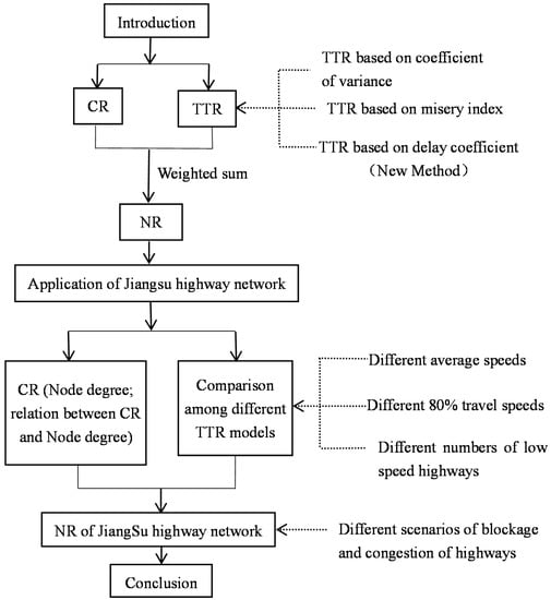
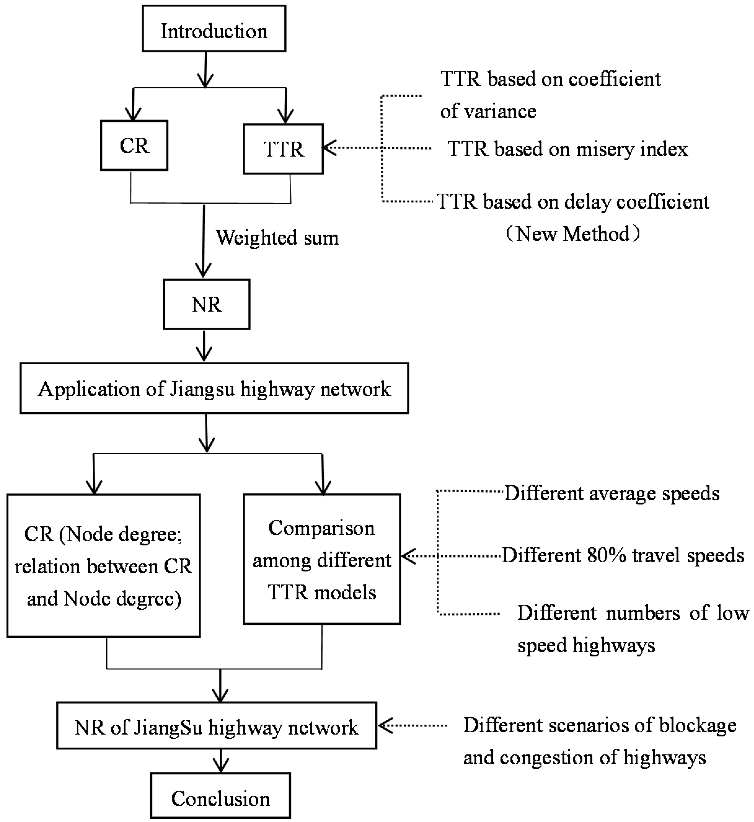
By building the dual topology model of a highway network in a certain area, the node degrees can be obtained in the topology network. The CR of the network was analyzed under random attack and deliberate attack. A new calculation method of TTR is proposed, and the change rule of the TTR of the road network was studied under a different travel time coefficient and delay coefficient. After comparison among different methods of TTR, the new method, named “TTR based on delay coefficient,” was verified. The method can be used in a large-scale highway network. Furthermore, the reliability of the road network was calculated under the different conditions of blockage and congestion. The structure of this research is shown in Figure 1.

Figure 1. The structure of this research.

As showed in Figure 1, methods based on the coefficient of variance and misery index are commonly used to calculate TTR. The two methods are expressed as Equation (4) in Section 3.2 and Equation (5) in Section 3.3. We propose the method based on the delay coefficient in Equation (9) in Section 4.1. Network connection reliability in complex network theory, shown as Equation (1) in Section 3.1, is used to calculate CR. The weighted sum of CR and TTR is NR, expressed as Equation (10) in Section 4.2. These reliability indexes can be applied in the Jiangsu highway network. The CR of the network when under deliberate attack or random attack was calculated and analyzed based on the topological network of the field network. These three TTR methods were compared when changing values of the average speed, 80% travel speed, and the number of low-speed highways. Therefore, the validity of the new method can be verified if it has a similar change rule. NR was also calculated under different block and congestion conditions to cognize the characteristic of highway network reliability.

2. Literature Review

Different probability distribution families could yield different values for the same measure of TTR. The probability mass function of the travel time in the road section was estimated by designing a kind of sampling process, and the distribution characteristics of travel time were analyzed under random and dynamic changes. Rakha et al. assumed that travel times follow a normal distribution and that segment travel times are independent. Their model demonstrated that computing the trip travel-time coefficient of variation provided estimates within 70% of trip travel-time variance for both uncongested and congested conditions [6]. Yang et al. found that specific selection of probability distribution families had few effects on measuring TTR. Lognormal distribution was the best fit among Weibull, gamma, normal, and lognormal distributions [7]. The proposed travel time estimation model captured the temporal pattern of travel time and its distribution well [8].

The application of TTR in a large-scale road network needs massive and dynamic survey data of traveling vehicles. The acquisition and processing of data is important to calculate TTR. GPS technology, digital maps, and Bluetooth technology are usually used to collect data. Woodard et al. introduced the Travel-Time Reliability: Issues and Proposed (TRIP) method to predict the probability distribution of travel time on an arbitrary route in a road network at an arbitrary time, using GPS data from mobile phones or other probe vehicles. TRIP provides improved interval predictions (forecast ranges for travel time) relative to Microsoft’s engine for travel time prediction as used in Bing Maps [9]. Hainen et al. estimated route choice and TTR with field observations of Bluetooth probe vehicles. It is useful for public agencies to assess mobility and TTR along alternate routes [10]. Guo calculated TTR in different periods by using the survey data of probe vehicles to establish an evaluation model of the operational efficiency in urban control systems [11]. Bhouri et al. evaluated the ramp metering impact based on traffic and TTR. The results indicated improvements in both aspects [12].

By using TTR, some researches were about designing the road network or finding the shortest path in the network. Sun et al. designed a new metric of TTR. Comparisons of TTR at the OD level were provided and the network reliabilities across multiple periods were also evaluated [13]. Uchida proposed the easier method because the number of unknown parameters was much smaller than that of the standard maximum likelihood estimation method [14]. Mittal et al. presented a networkwide evaluation of the effect of connectivity on TTR. A maximum entropy multi-criteria user equilibrium (ME-MUE) model was more consistent with the real trip process in that the reliable travel time was increasing with decreasing travel distance in the routes used, and the road traffic was smoother when using the ME-MUE model to design the road network [15,16]. Xu selected the indicators CR, TTR, and capability reliability as the optimization goals of the design problems in the urban road network, and established continuous models of the urban road network [17]. Zhi et al. used the reliability of travel time as the weight of path selection via the Dijkstra algorithm, and the method reflected the actual vehicle path selection more accurately [18]. Chen et al. proposed a deviation path algorithm to solve the K reliable shortest paths (KRSP) problem in large-scale networks. The A* technique was introduced to further improve the KRSP finding performance [19]. A small number of methods was used to calculate TTR in freight transportation, but not in passenger transportation. For the value of reliability (VOR), Shams et al. indicated that the estimated VOR values varied largely from one study to another, probably due to the use of different units, reliability measures, and survey design approaches [20].

Bai summarized the reliability indexes of travel time, such as variation coefficient, buffer time, tardy trip, and travel time distribution reliability. From the three perspectives of travel time boundary, buffer time, and delay time, travel time measures were estimated from average travel time and 95th travel time [21]. Schroeder et al. presented a methodology for incorporating freeway reliability analysis in the Highway Capacity Manual. The methodology uses a scenario-based approach [22].

In summary, connection reliability describes the static structure character, or connection probability, between two nodes in an abstract network. The calculation of TTR needs to process a large amount of data due to the huge number of vehicles running on the highways. Specific selection of probability distribution families has little effect on measuring TTR. It is difficult to accurately calculate TTR if all vehicle speeds on the different road grades are counted all together to obtain the average speed. Therefore, some NR methods, such as TTR based on the coefficient of variation, are effectively applied in individual roads, but they are usually not reasonable in a large-scale road network. The misery index can be used to calculate the weighted sum of each road misery index as the TTR of the road network. However, the weighting method is unclear.

3. Reliability Indexes of a Complex Highway Network

The indexes of a complex network include node degree, intermediary centrality, proximity centrality, average path length, aggregation coefficient, network global efficiency, invulnerability, reliability, and so on [23,24]. Node degree $k\left(v_i\right)$ is the number of nodes connected directly to the $i$th node. Average path length $d$ is the average of the edge numbers in the shortest paths between any two points divided by the total edge number. We introduced the main indexes, such as reliability indexes, including CR, TTR, and NR.

3.1. Connection Reliability

Connection reliability can be defined as the probability that at least one path is connected between any two nodes in the road network [25,26]. As long as there is a path between any two points in the whole network, the network will be reliable to some extent. The equation is as follows:

$$R_C=\frac{{{\displaystyle \sum }}_{i=1}^{\omega }{N}_i\left(N_i-1\right)}{\omega {{\displaystyle \sum }}_{i=1}^{\omega }{N}_i\left(N_i-1\right)d_i}$$

(1)

where $R_C$ is the network connection reliability $0\le R_C\le 1$. The value of $R_C$ is 1 when the network is fully connected, $\omega$ is the number of subnets formed after the node is removed, $N_i$ is the number of nodes that connect to the $i$th subnet, and $d_i$ is the average shortest path of the $i$th subnet—that is to say, the sum of the edge numbers in the shortest paths between any two points is divided by the total edge number.

3.2. TTR Based on the Coefficient of Variation

The method calculates the travel time based on mathematical statistics, and uses the coefficient of variation as the TTR [27]. The reliability equations are as follows:

$$S\left(t\right)=\frac{1}{n}{\displaystyle \sum }_{i=1}^n{\left(t_i-\overline{t}\right)}^2$$

(2)

$$\sigma =\sqrt{S}$$

(3)

$$CV(t)=\frac{t_d-\sigma }{\overline{t}}$$

(4)

where $S\left(t\right)$ is the variance in travel times, $n$ is the number of statistical vehicles, $t_i$ is the travel time of the $i$th vehicle, and $\overline{t}$ is the average travel time of all vehicles. $\sigma$ is the standard deviation of travel times, and $CV\left(t\right)$ is the coefficient of variation. $t_d$ is defined as the unit blockage time close to the blocking status.

The TTR model based on the coefficient of variation uses the average travel time of all vehicles. Although all vehicles run smoothly on the road network, the field speeds of vehicles are significantly different if the designed speeds of roads are varied. Therefore, it is difficult to reflect the objective operation state by using the average travel time $\overline{t}$. The TTR model based on the coefficient of variation is reasonable for calculating the single road, but not feasible for calculating the whole road network.

3.3. Misery Index

The misery index can be calculated by taking data from the worst 20% of data and finding the average travel time for just those trips. The misery index reflects the relative distance between the average travel time of the 20% most unlucky travelers and the average travel time of all travelers [28]. It is defined as follows:

$$MI=\frac{M_{\left(t_i>t_{80\%}\right)}-\overline{M}}{\overline{M}}\times 100\%$$

(5)

where $MI$ is the misery index, $M\left(t_i>t_{80\%}\right)$. is the average travel time of the longest 20% of all trips, and $\overline{M}$ is the average travel time.

The influence of different path length on travel time can be eliminated by using the coefficient of variation. Usually, the misery index is used to evaluate the impact of accidental factors on travel time. The misery index is an effective measure of the TTR of a single road. In the field, the road network is composed of roads of different grades, and the same distance will take significantly different travel hours on different grades of roads. Therefore, it is difficult to calculate the TTR of the whole road network.

4. A New Method of TTR

The BPR (Bureau of Public Road) function calculates the travel time of a single road section, but does not reflect its reliability directly. Equations (4) and (5) are effective in calculating the TTR of individual roads; however, they are not reasonable for a large-scale road network. In road networks, different grades of roads usually have different design speeds. If using the average speed directly, the reliability of the field traffic network cannot be accurately calculated because of different speed limits.

With consideration of the limitations of the above methods, a new method based on the delay coefficient is proposed in order to accurately describe the highway NR. By calculating the relevant ratio of travel time, this method eliminates the influence of different speed limits on different road grades.

4.1. TTR Based on the Delay Coefficient

The travel time of the unit distance can be obtained by use of the maximum speed limit, which is regarded as the minimum unit travel time $t_{i,\min }$ for the $i$th highway ($i=1,\dots ,n,n$ is the number of roads). Using the average travel speed of each highway, the unit travel time $t_i$ can also be calculated. The relevant ratio of the unit travel time $t_i$ to the minimum unit travel time $t_{i,\min }$ of the highway is called the travel time coefficient ${\mathsf{\Delta }}_i$. The average value ${\mathsf{\Delta }}_x$ of all ${\mathsf{\Delta }}_i$ is shown as Equation (6). $t_d$ is defined as the unit blockage time close to the blocking status (for example, the average vehicle speed is 10 km/h). The travel time coefficient ${\mathsf{\Delta }}_d$, called the blockage coefficient, is calculated similarly using Equation (7). The ratio of the 80% travel time $t_{i,80}$ (the 80th percentile value of the travel time distribution, as in Equation (5)) to the minimum unit travel time $t_{i,\min }$ is called the delay coefficient ${\mathsf{\Delta }}_{i,80}$ of the ith highway. The average value is ${\mathsf{\Delta }}_{x,80}$, shown in Equation (8). Finally, TTR $R_t$ is calculated by ${\mathsf{\Delta }}_x$, ${\mathsf{\Delta }}_d$, and ${\mathsf{\Delta }}_{x,80}$, which is shown in Equation (9).

$${\mathsf{\Delta }}_x=\frac{1}{n}\sum _{i=1}^n{\mathsf{\Delta }}_i=\frac{1}{n}\sum _{i=1}^n\frac{t_i-t_{i,\min }}{t_{i,\min }}$$

(6)

$${\mathsf{\Delta }}_d=\frac{1}{n}\sum _{i=1}^n\frac{t_{i,d}-t_{i,\min }}{t_{i,\min }}$$

(7)

$${\mathsf{\Delta }}_{x,80}=\frac{1}{n}\sum _{i=1}^n\frac{t_{i,80}-t_{i,\min }}{t_{i,\min }}$$

(8)

$$R_t=1-\sqrt{\frac{{\mathsf{\Delta }}_x+{\mathsf{\Delta }}_{x,80}}{2{\mathsf{\Delta }}_d}}$$

(9)

In the equations, ${\mathsf{\Delta }}_x$ is the travel time coefficient, ${\mathsf{\Delta }}_d$ is the blockage coefficient, ${\mathsf{\Delta }}_{x,80}$ is the delay coefficient, $t_i$ is the unit travel time of the $i$th highway, $t_{i,min}$ is the minimum unit travel time of the $i\mathrm{th}$ highway, $t_{i,d}$ is the unit blockage time of the $i$th highway, $t_{i,80}$ is the 80% travel time of the ith highway, and $R_t$ is TTR.

The travel time variation and the ratio of actual travel time and ideal travel time are used in the model. This can eliminate the influence of absolute difference of the different design speeds and the different travel time. Therefore, the method can be used in a road network with different grades of roads.

TTR is related to the number of low-speed roads, the travel coefficient, and the delay coefficient, whereas CR depends on the node degree of the blocking highways.

4.2. The Hybrid Reliability of a Highway Network

CR and TTR represent the reliability of the network structure character and the traffic operation character, respectively. The field road network can be represented by NR, and weighted by the CR and TTR. The equation of road NR $R$ is as follows:

$$R={\alpha }_c{R}_c+{\alpha }_t{R}_t$$

(10)

where ${\alpha }_c$ is the weight of CR, ${\alpha }_t$ is the weight of TTR, and ${\alpha }_c+{\alpha }_t=1$.

Sumalee et al. found that the weight of TTR ${\alpha }_t$ was relativity large at 0.625 when a sudden traffic jam occurred, and the weight of CR ${\alpha }_c$ was relatively large at 0.691 when a natural disaster caused a road blockage [29].

5. Calculation of the Highway Network Topology Index

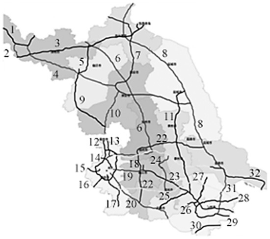
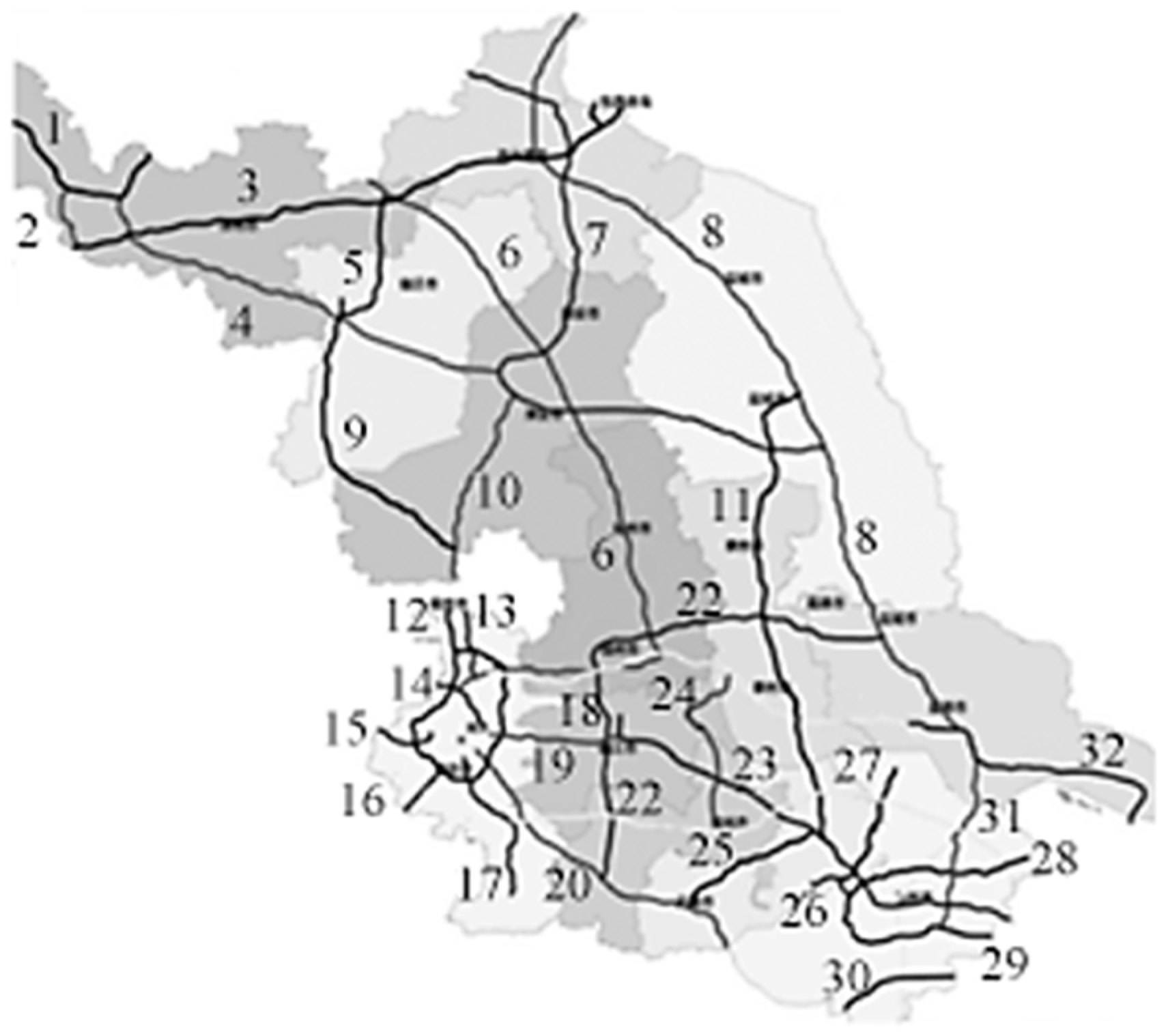
The Jiangsu highway network is shown in Figure 2, in which 32 highways are marked. Jiangsu province has a developed economy in China. Its road network density and highway level are relatively high. The maintenance and management of the highway network are important work for the transportation administration department. TTR is one of the focus indexes.

Figure 2. Highway network in Jiangsu province.

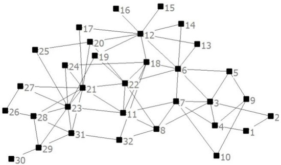
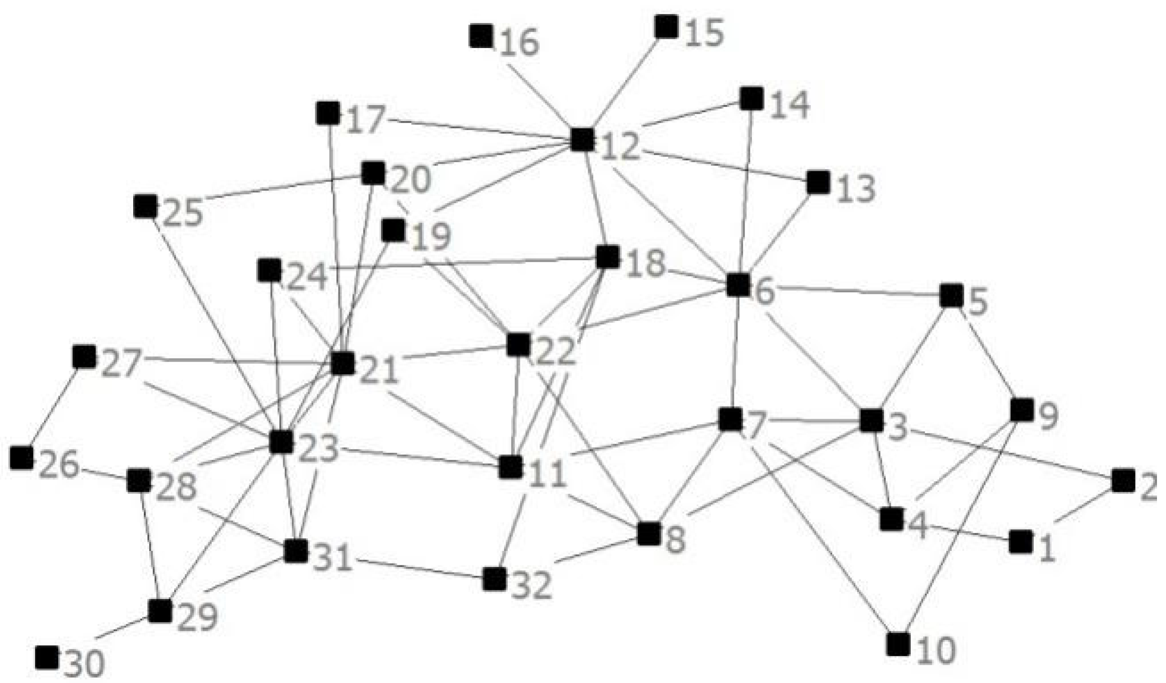
The topological structure of the regional highway network was obtained with a dual method, as shown in Figure 3. The highway was regarded as the network node, and the connection relationship between them was regarded as the edge of the network.

Figure 3. Dual topological graph of the highway network.

The Ucinet software, a comprehensive package for the analysis of social network data as well as other 1-mode and 2-mode data that can handle a maximum of 32,767 nodes, was used to calculate the node degree of each highway in the topological network, and the results are shown in Table 1.

Table 1. Node degrees of the highway network.

Node	Degree	Node	Degree	Node	Degree	Node	Degree
1	2	9	3	17	2	25	2
2	2	10	2	18	6	26	2
3	6	11	6	19	3	27	3
4	4	12	9	20	4	28	5
5	3	13	2	21	9	29	4
6	8	14	2	22	7	30	1
7	6	15	1	23	9	31	5
8	5	16	1	24	3	32	3

CR reflects the structure character and TTR reflects the traffic operation. By using different methods and designing some scenarios under random attacks and deliberate attack circumstances, we found the change rule of CR and the TTR of the highway network. The highway NR in the region could be comprehensively evaluated.

6. Connection Reliability Analysis of a Highway Network

6.1. Network Connection Reliability under Random Attack and Selected Attack

In complex networks, an “attack” refers to the failure or break of edges. In a highway network, an attack can be regarded as the failure or break of the highway, including highway damage caused by natural disasters, highway blockage caused by traffic accidents or serious traffic congestion, closure caused by construction and maintenance of the highway, or even highway damage caused by terrorist attacks. The selected attack is a kind of malicious damage aimed at the highway network structure, which quickly paralyzes the highway network, whereas a random attack does not choose a specific highway, but rather randomly attacks one by one, finally leaving the highway network paralyzed.

The network connection reliability is calculated by removing nodes one by one under a random attack or selected attack. Nodes are removed in the order of 32 randomly generated numbers under a random attack, whereas nodes are removed in order of node degree from large to small under a selected attack.

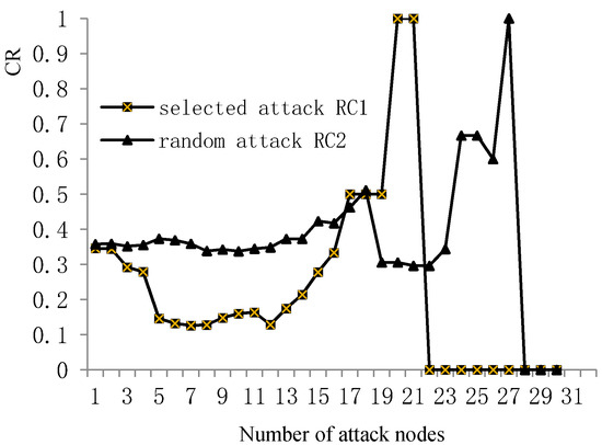
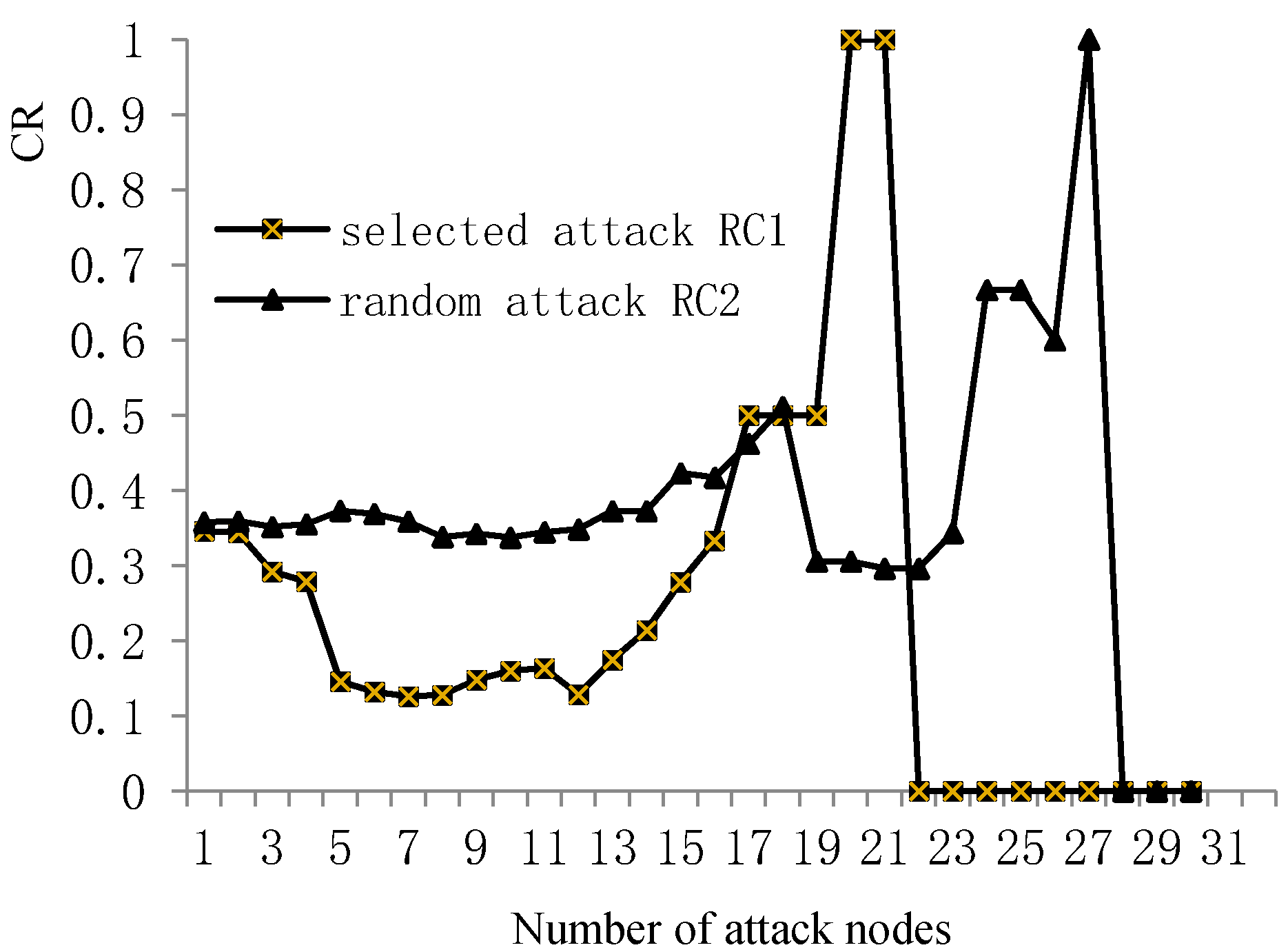
Highway network paralysis is a certain type of failure state in which all nodes are isolated—that is to say, all highways are disconnected. Figure 4 shows that in a network connection reliability under random attack, RC2 was reduced to 0 after 28 steps, whereas for the network connection reliability under selected attack, RC1 = 0 after 22 steps. The connection reliability RC1 under selected attack was always lower than that under random attack within 16 steps. Starting from step 17, the remaining network under selected attack was composed of three two-node subnets, whereas the remaining network under random attack was a connected subnet with 11 nodes.

Figure 4. CR of the network under selected attack or random attack.

To sum up, the CR of the highway network was greatly reduced when the nodes with a high node degree were selectively removed. When the nodes were removed stochastically, the network connection reliability decreased more slowly than under selected attack. It can be seen that the highways represented by high-degree nodes were more important to the regional highway NR than other highways, and the blockage of these important highways had a serious impact on the whole highway network structure.

6.2. Network Connection Reliability of Removing Multiple Nodes

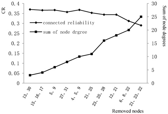
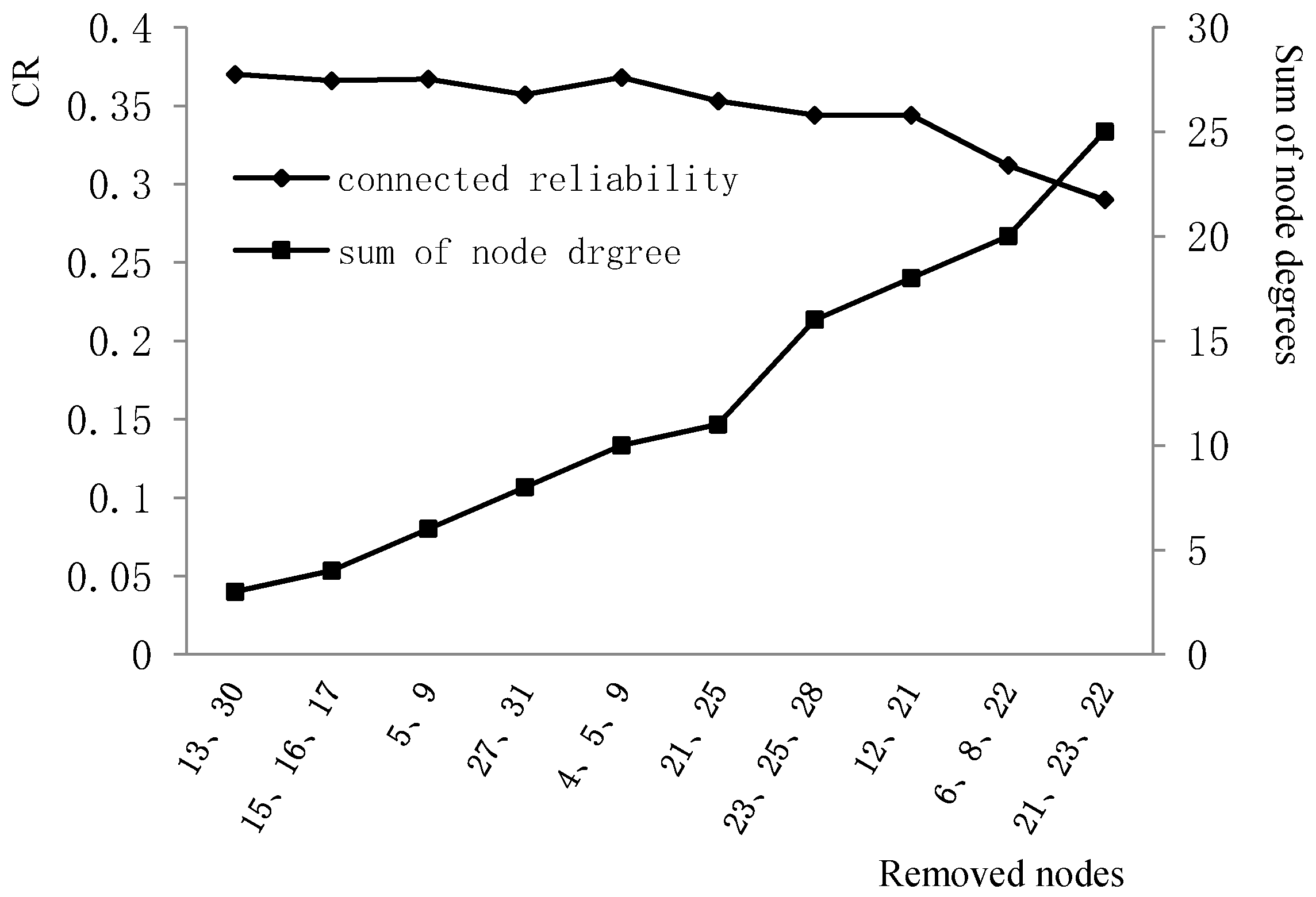
The above attacks against the network were to remove the nodes one by one. One highway blockage in the network will cause the blockage of other highways in turn, or the destruction of the highways one by one. In the field highway network, traffic accidents or natural disasters always cause a large area of traffic jam, resulting in the blockage of several highways. After designing the following simulation scenarios of a several-highway blockage, the sum of the node degrees of the blocked highways was statistically calculated. The network connection reliability was calculated and analyzed as shown in Figure 5.

Figure 5. Correlation of the connection reliability and node degree after deleting some nodes.

From Figure 5, it can be seen that the network connection reliability had an obvious downward trend with an increase in the sum of the removed node degrees. Therefore, increasing the number of highways, especially highways with a large node degree, is an effective measure to improve the CR of a highway network. In the field network, the number of highway in the southern region was obviously different than that in the northern region. The highway mileage in the southern region accounted for more than half of the total mileage, whereas the area in the northern region occupied about one third of the total area. The node degrees and CR in the southern region were higher than those in the northern region. Therefore, the reliability of the regional highway network can be improved by increasing the density of the highway network or increasing the connection of highways in the northern region.

7. TTR Using Different Methods

Connection reliability reflects the overall structure character in the highway network. TTR is used to reflect NR based on the different vehicle running speeds. The relationship between the average speed and the variance of speeds can be derived. Therefore, different TTR methods can be calculated and compared based on the same road network and traffic flow status. We applied three methods in the highway network of Jiangsu province.

In Equation (4), $\overline{t}$ is the average travel time of all vehicles in the road network. The variable needs to be substituted in Equation (4) to calculate the TTR. The speed limits are different for different grades of roads. Therefore, vehicle speeds of different roads show significant differences. It is inappropriate to use the average travel time in the same equation if the model is used in a network composed of different grades of roads. There is the same flaw with $M\left(t_i>t_{80\%}\right)$ in Equation (5). Therefore, Equations (4) and (5) are feasible for individual roads or roads of the same grade in a network, but are not feasible for a network with different grades of roads. For the new method, $t_i$ is the unit travel time of the $i$th highway in Equation (6). $t_{i,min}$ is the minimum unit travel time of the $i\mathrm{th}$ highway. These variables for different grades of roads can be calculated by using the relevant ratio of the unit travel time $t_i$ to the minimum unit travel time $t_{i,\min }$. Equations (6)–(9) were designed to avoid the flaw existing in Equations (4) and (5). With the new method, Equation (9) can be used in a network composed of different grades of roads.

Taking all the vehicles in the highway network during the survey time as the statistical object, the unit travel time of each highway can be obtained by calculating the average vehicle speed. The average value and variance of the unit travel time can be obtained for each highway correspondingly. The total average value and the total variance can be calculated, which are related to the average and variance of the unit travel time, respectively. The detailed derivation process is shown in the following section.

7.1. Speed Average and Variance in the Network of Different Grades of Highways

The vehicle speeds in the highway network are assumed to follow a normal distribution. When the maximum speed limit and the blocking speed are given, TTR $R_t$ is only related to the vehicle speed on each highway.

It is supposed that there are $m$ highways in a highway network. The number of vehicles on each highway is $n_1$, $n_2$, $n_3$, $n_4$, $n_5$, …, $n_m$. By statistical calculation, the average speeds of each highway are $\overline{x_1}$, $\overline{x_2}$, $\overline{x_3}$, $\overline{x_4}$, $\overline{x_5}$, …, $\overline{x_m}$, and the speed variances of vehicles on each highway are $S_1$, $S_2$, $S_3$, $S_4$, $S_5$, …, $S_m$. After all the vehicle data are mixed, the average speed and speed variance of all vehicles are solved as follows.

$$\overline{X}=\frac{n_1\overline{x_1}+n_2\overline{x_2}+\dots +n_m\overline{x_m}}{n_1+n_2+\dots +n_m}=\frac{{\displaystyle {\displaystyle \sum }_{i=1}^m}{n}_i\overline{x_i}}{{\displaystyle {\displaystyle \sum }_{i=1}^m}{n}_i}$$

(11)

where $\overline{X}$ denotes the average speed of the total vehicles.

Therefore, the speed variance of each highway can be expressed as:

$$S_k=\frac{1}{n_k}{{\displaystyle \sum _{i=1}^{n_k}\left(x_{k,i}-\overline{x_k}\right)}}^2=\frac{1}{n_k}{\displaystyle \sum _{i=1}^{n_k}{x}_{k,i}{}^2-{\overline{x_k}}^2}$$

(12)

where $S_k$ is the speed variance of the $k$th highway, $n_k$ is the number of vehicles on the $k$th highway, and ${\overline{x}}_k$ is the average speed of all vehicles on the $k$th highway.

The overall speed variance can be expressed as:

$$S=\frac{{\displaystyle \sum _{i=1}^m{\displaystyle \sum _{j=1}^{n_i}{x}_{ij}^2}}}{{\displaystyle \sum _{i=1}^m{n}_i}}-{\overline{X}}^2=\frac{{\displaystyle \sum _{j=1}^{n_1}{x}_{1j}^2}+{\displaystyle \sum _{j=1}^{n_2}{x}_{2j}^2}+\dots +{\displaystyle \sum _{j=1}^{n_m}{x}_{mj}^2}}{{\displaystyle \sum _{i=1}^m{n}_i}}-{\overline{X}}^2=\frac{{\displaystyle \sum _{i=1}^m{n}_i\left(S_i+{\overline{x_i}}^2-\overline{x_i}\right)}}{{\displaystyle \sum _{i=1}^m{n}_i}}$$

(13)

It is supposed that the number of vehicles on each highway is the same. When $n_1=n_2=\dots =n_m$, the average speed value and variance after mixing can be expressed as follows:

$$\overline{X}=\frac{{\displaystyle {\displaystyle \sum }_{i=1}^m}\overline{x_i}}{m}$$

(14)

$$S=\frac{1}{m}{\displaystyle \sum _{i=1}^m\left(S_i+{\overline{x_i}}^2\right)}-{\left(\frac{{\displaystyle \sum _{i=1}^m\overline{x_i}}}{m}\right)}^2=\frac{1}{\mathrm{m}}{\displaystyle \sum _{i=1}^m{S}_i}+\frac{1}{\mathrm{m}}{\displaystyle \sum _{i=1}^m{\overline{x_i}}^2}-\overline{X}=\frac{1}{\mathrm{m}}{\displaystyle \sum _{i=1}^m{S}_i}+S^{\prime }$$

(15)

where $S$ is the speed variance of all vehicles in the whole road network, and $S^{\prime }$ denotes the variance of the average speed of each highway.

7.2. TTR with Different Travel Time Coefficients

When the maximum speed limit and the blocking speed are given, TTR $R_t$ is only related to the vehicle speed on each highway, which is reflected in ${\mathsf{\Delta }}_x$ of Equation (8) and ${\mathsf{\Delta }}_{x,80}$ of Equation (10). Therefore, it can be divided into two cases: the TTR of the congested highway with different travel time coefficients and the one with different delay coefficients.

Given the average vehicle speed $v_d=10\mathrm{km}/\mathrm{h}$ close to the blocking state, the maximum speed limit of each highway is 120 km/h. The unobstructed speed of all highways is 110 km/h. The blocking coefficient is calculated as ${\mathsf{\Delta }}_d=11$ using Equation (7). One or more of the highways are in the “low speed status,” whose speeds are regarded as between 10 km/h and 110 km/h. The TTR can be calculated by using Equation (9), and at this point, CR of the highway network does not change.

Assuming that the vehicle velocities follow normal distribution, the 80% speed $v_{i,80}$ of all highways is 50 km/h, and the variance of unit travel times can be calculated as 0.605 min². The average speed of each highway vehicle is 70 km/h, 90 km/h, and 110 km/h, and the variance is 0.166 min², 0.401 min², and 0.508 min², respectively. With the vehicle speeds on some highways changing and the number of low-speed highways increasing gradually, the travel time reliabilities of the highway network can be calculated. The results are shown in Table 2 using different methods.

Table 2. TTR of the highway network with different numbers of low-speed highways (partial).

Number of Low-Speed Highways		Travel Time		TTR
$v_i$ = 70 km/h $v_{i,80}$ = 50 km/h	$v_i$ = 110 km/h $v_{i,80}$ = 50 km/h	Total Average (min)	Total Variance (min2)	Delay Coefficient	Coefficient of Variation	Delay Travel Index
1	31	0.555	0.594	0.738	1.390	0.221
2	30	0.565	0.584	0.736	1.353	0.206
3	29	0.574	0.572	0.735	1.317	0.198
…	…	…	…	…	…	…
28	4	0.818	0.231	0.696	0.588	0.102
29	3	0.828	0.215	0.694	0.560	0.101
30	2	0.838	0.199	0.693	0.532	0.103
31	1	0.847	0.182	0.691	0.504	0.103
32	0	0.857	0.166	0.690	0.475	0.104

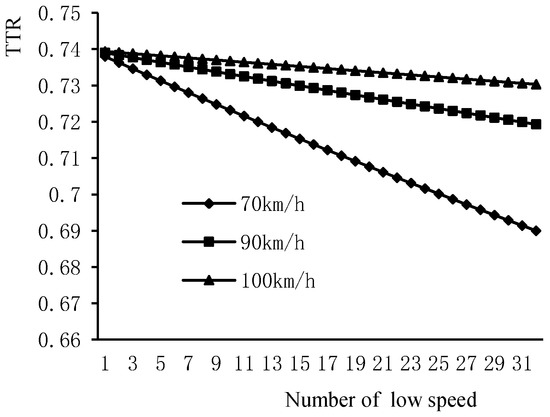
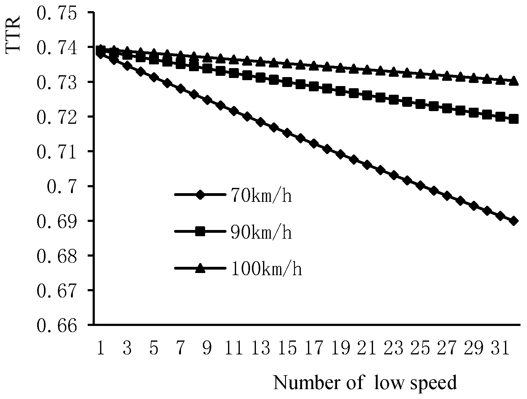
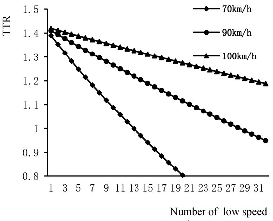
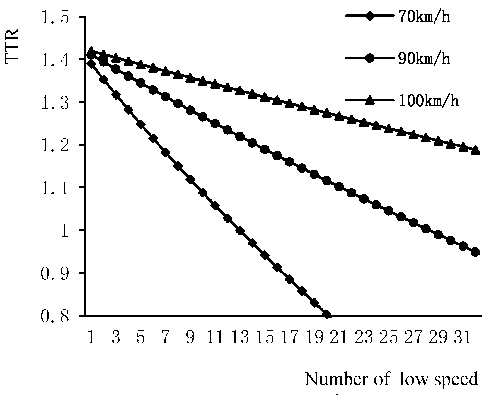
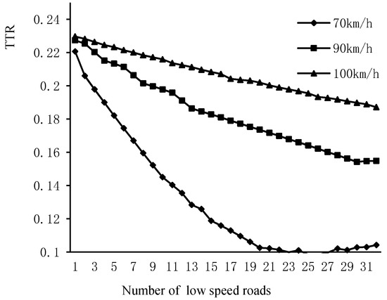
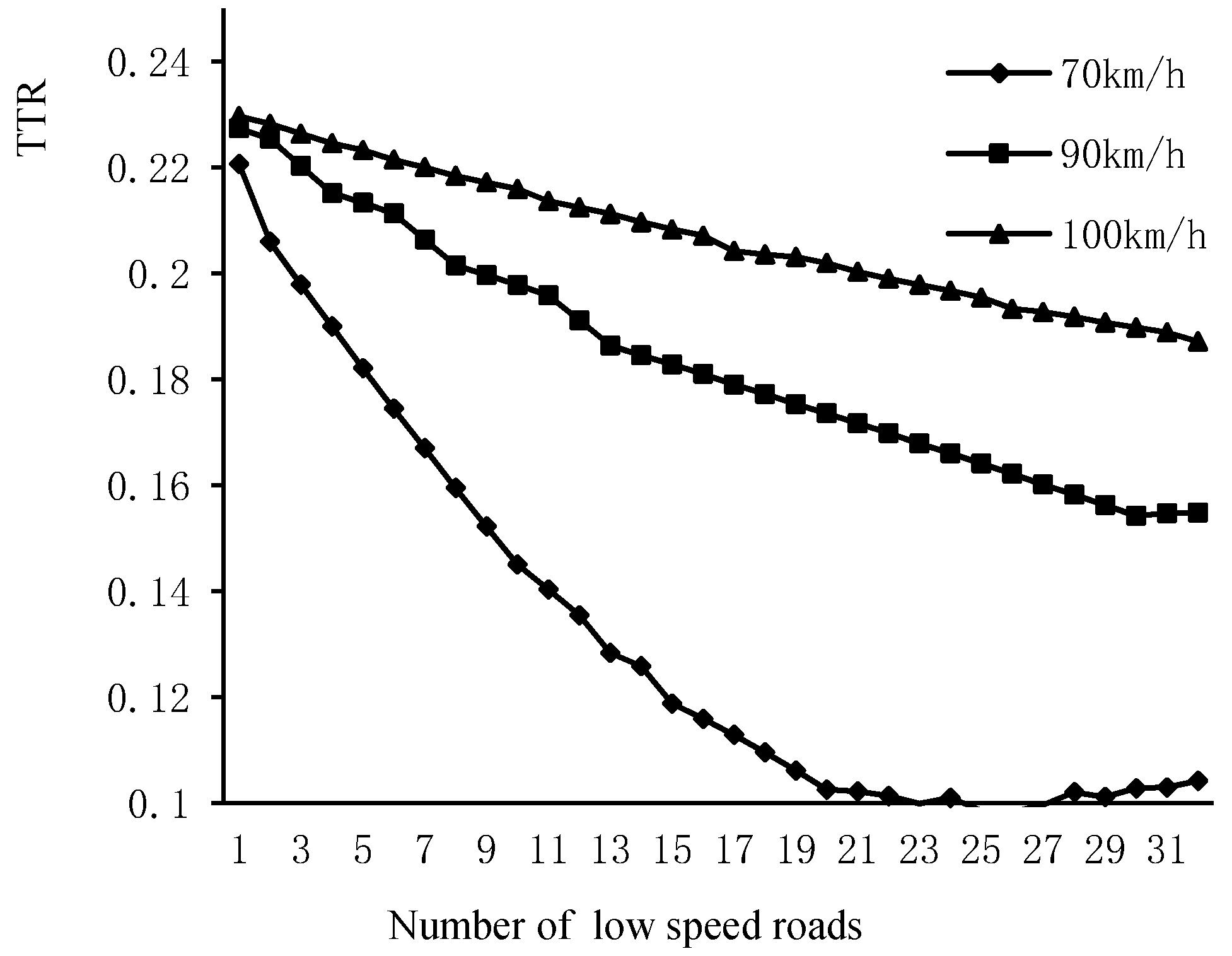
By using different methods of TTR, including Equations (4), (5) and (9), the calculation values can be shown, as in Figure 6, Figure 7 and Figure 8.

Figure 6. TTR based on the delay coefficient, Equation (9) ($v_i$ = 70, 90, 100 km/h).

Figure 7. TTR based on the coefficient of variation, Equation (4) ($v_i$ = 70, 90, 100 km/h).

Figure 8. TTR based on the misery index, Equation (5) ($v_i$ = 70, 90, 100 km/h).

As shown in Figure 6, the TTR values varied in a narrow range from 0.68 to 0.74. That is to say, when the average speed was reliably high, the TTR was high despite many low-speed highways. Under the condition that the delay coefficient does not change, TTR decreased with the increase in the number of low-speed highways, and the TTR of the highway network decreased with the increase in the travel time coefficient. When the speed was 90 km/h, the TTR of the highway network decreased slowly even if there were many low-speed highways. TTR was still 0.719 even when the average speed on all highways was 90 km/h. When the average speed was 70 km/h, the TTR was 0.69 and the network operation was relatively reliable. However, when the speed continuously decreased, the TTR of the highway network had a trend of quickly decreasing, which was also in line with the field traffic status of the highway network.

By comparing Figure 6, Figure 7 and Figure 8, it can be seen that under the condition of the constant delay coefficient, TTR (9) had the same changing trend as the coefficient of variation (4) and misery index (5) when the travel time coefficient changed. When the travel time coefficient became the minimum, the vehicle speed on all highways reached the unobstructed speed of 110 km/h. The TTR of Equations (4), (5) and (9) all reached the maximum value. With the increase in the number of low-speed highways, TTR decreased and the change rules of three indexes were similar.

7.3. TTR with Different Delay Coefficients

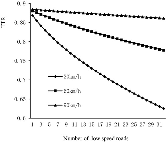
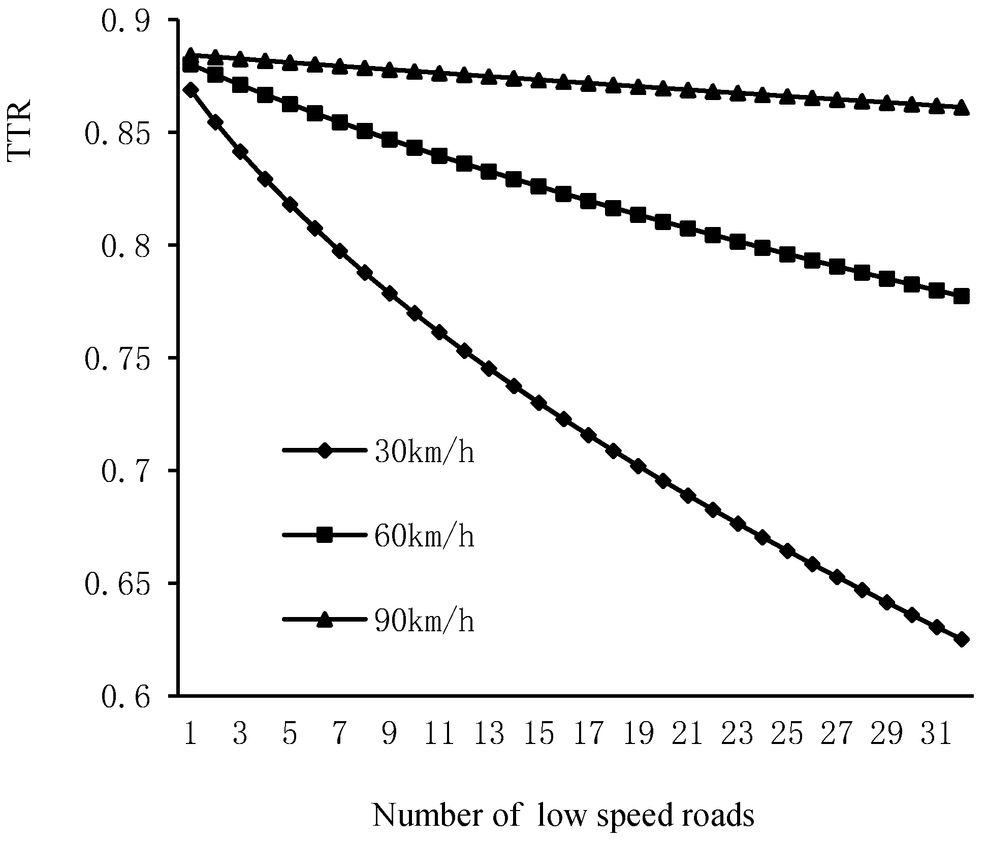
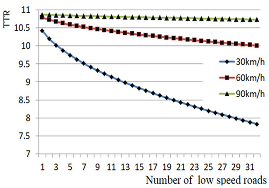
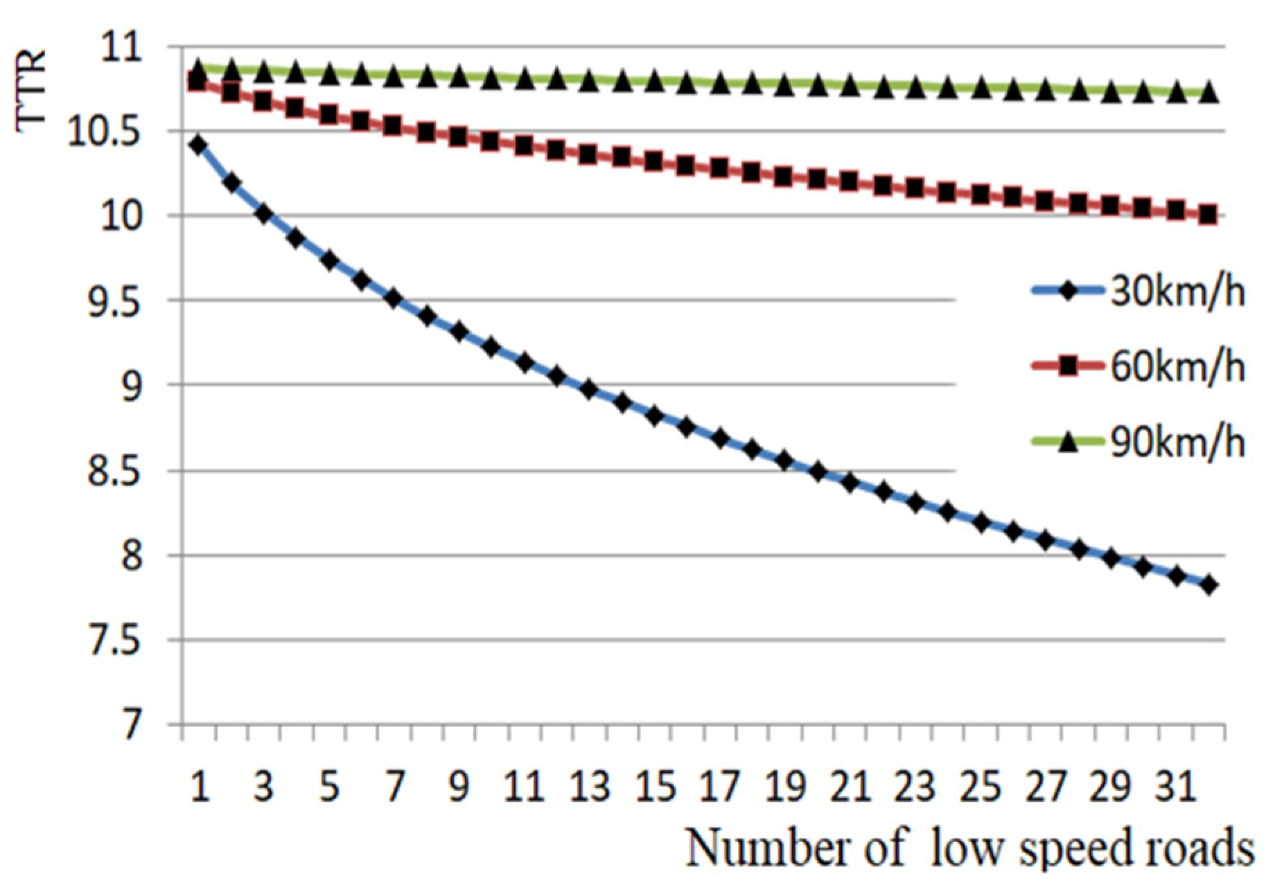
When the average speed of the highway network was set to 110 km/h, that is, the average unit travel time of all highways was 0.545 min and the variance of unit travel time varied with the variance of the unit travel time, the variations in the TTR by use of different methods were calculated and are shown in Figure 9, Figure 10 and Figure 11.

Figure 9. TTR based on the delay coefficient, Equation (9) ($v_{i,80}$ = 30, 60, 90 km/h).

Figure 10. TTR based on the coefficient of variation, Equation (4) ($v_{i,80}$ = 30, 60, 90 km/h).

Figure 11. TTR based on the misery index, Equation (5) ($v_{i,80}$ = 30, 60, 90 km/h).

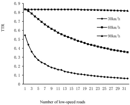
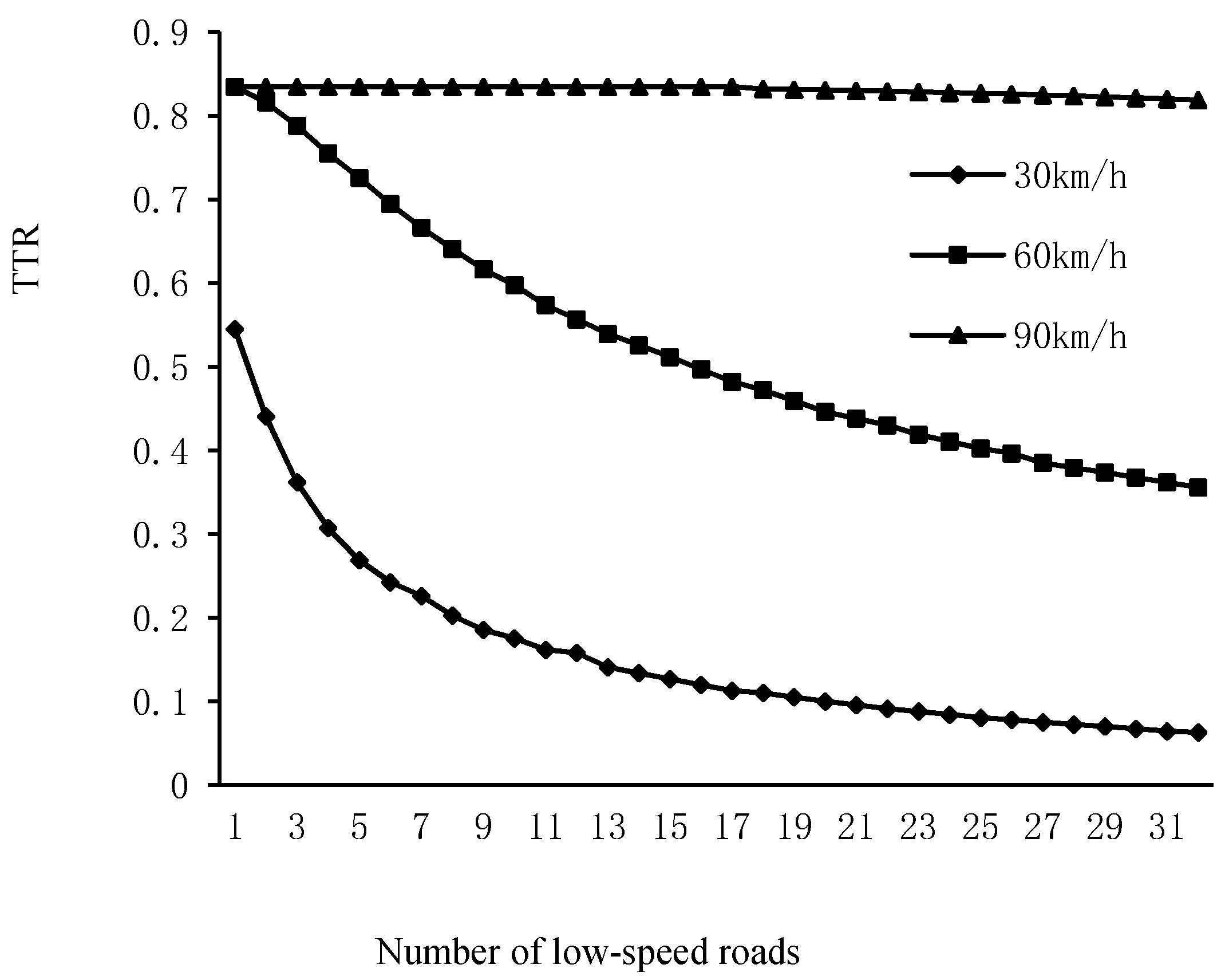
Figure 9 shows that TTR of the highway network decreased along with the increase in the number of low-speed highways when the travel coefficient was constant. The highway network TTR decreased as the delay coefficient increased, or $v_{i,80}$ decreased. There were multiple roads in the low-speed status when $v_{i,80}$ was 90 km/h, and the TTR of the road network did not greatly decrease. Even when all roads were in the low-speed status, the TTR was still 0.861 and the road network operation was relatively reliable. When $v_{i,80}$ decreased, the TTR of the road network had a tendency to drop quickly, which was in line with the field traffic conditions.

By comparing Figure 9 with Figure 10 and Figure 11, it was found that under the condition of the constant travel time coefficient, when the delay coefficient changed, the TTR showed the same trend as the coefficient of variation and misery index. When the delay coefficient was the minimum, that is, when $v_{i,80}$ of all roads in the highway network reached 100 km/h, the travel time reliabilities of Equations (4), (5) and (9) reached the maximum value. The three methods had the same change rule. The reliability method of travel time based on the delay coefficient was verified.

7.4. TTR with Different Travel Time Coefficients and Delay Coefficients

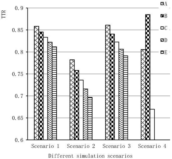
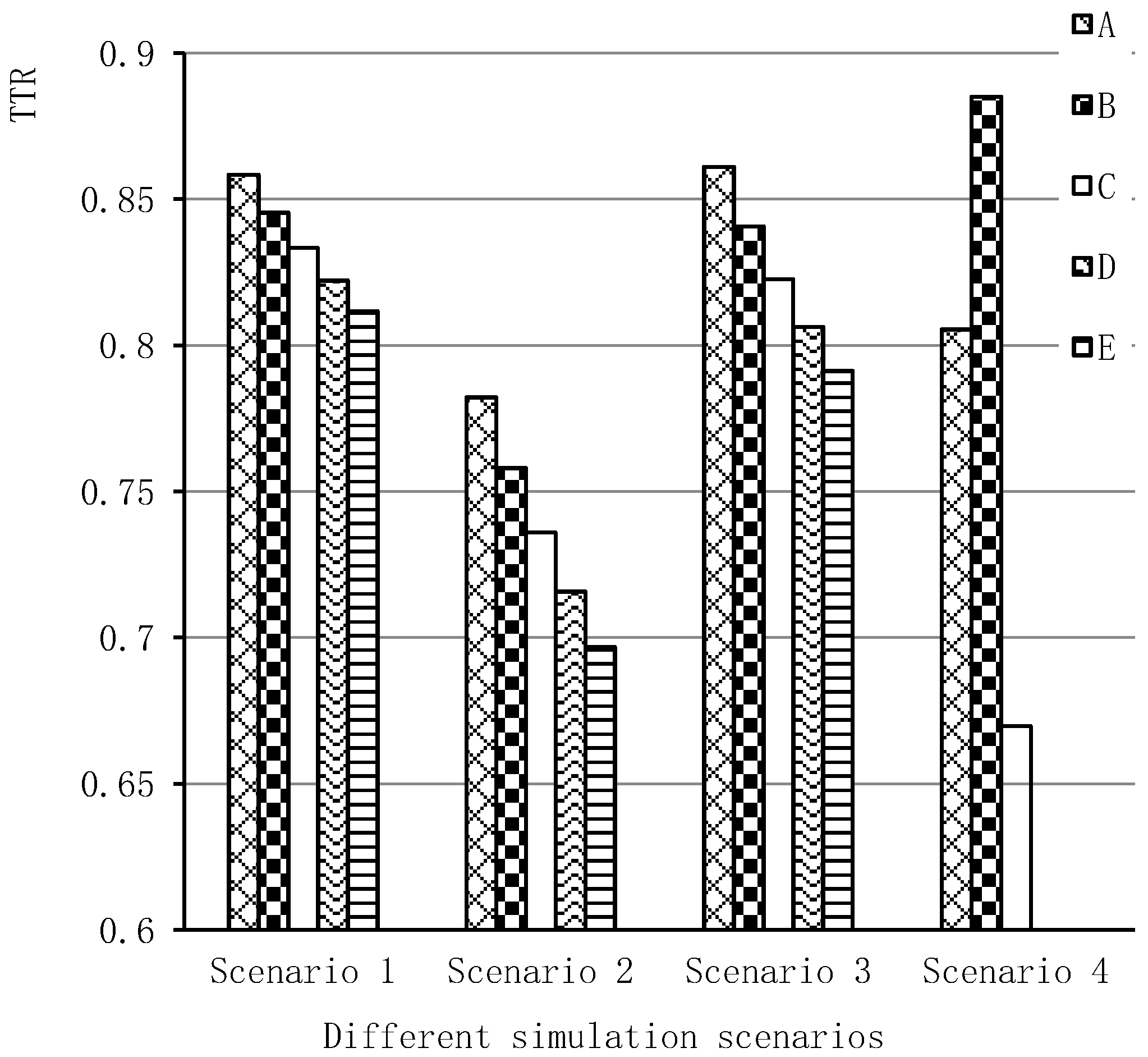
When the average speed was 60 km/h, 90 km/h, and 110 km/h, the average 80% travel speed $v_{i,80}$ was 50 km/h, 80 km/h, and 100 km/h, respectively. At this time, the average unit travel time of the highway network was 1, 0.667, and 0.545 min, respectively, and the corresponding variance was 0.0566, 0.0098, and 0.004225 min², respectively. The TTR varied along with the number of low-speed roads, as shown in Table 3 and Figure 12.

Table 3. TTR based on the delay coefficient.

Simulation Scenario		Number of Low-Speed Roads			TTR
		$v_{i,80}$ = 50 km/h $v_i$ = 60 km/h	$v_{i,80}$ = 80 km/h $v_i$ = 90 km/h	$v_{i,80}$ = 100 km/h $v_i$ = 110 km/h	Delay Coefficient Equation (9)
Scenario 1	A	1	5	26	0.858
	B	1	10	21	0.845
	C	1	15	16	0.833
	D	1	20	11	0.822
	E	1	25	6	0.812
Scenario 2	A	5	25	2	0.782
	B	10	20	2	0.758
	C	15	15	2	0.736
	D	20	10	2	0.716
	E	25	5	2	0.697
Scenario 3	A	1	4	27	0.861
	B	2	8	22	0.841
	C	3	12	17	0.823
	D	4	16	12	0.806
	E	5	20	7	0.791
Scenario 4	A	0	32	0	0.805
	B	0	0	32	0.885
	C	32	0	0	0.670

Figure 12. TTR based on the delay coefficient.

As shown in Figure 12, the TTR of highway network decreased when the number of low-speed highways increased. Scenario 4 shows that when the average travel speed $v_i$. and 80% speed $v_{i,80}$ of the highway network were largest in the three conditions, the reliability of the travel time of the highway network was the greatest reliability. When both $v_i$ and $v_{i,80}$ were the smallest, the difference of the TTR was obviously smallest under all conditions. By comparing to the other three simulation scenarios, it can be seen that TTR had a slight change from 0.697 to 0.861 when the number of highways of $v_i$ and $v_{i,80}$ was much the same.

8. Highway NR under Blockage and Congestion States

When traffic jams or serious natural disasters result in highway blockage, travelers pay different attention to connection reliability. When traffic jams occur, people pay more attention to travel time, whereas when highway blocks occur, they are more concerned with highway network accessibility.

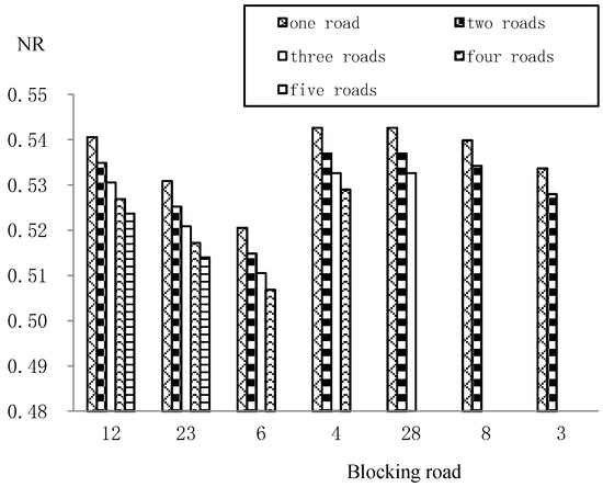
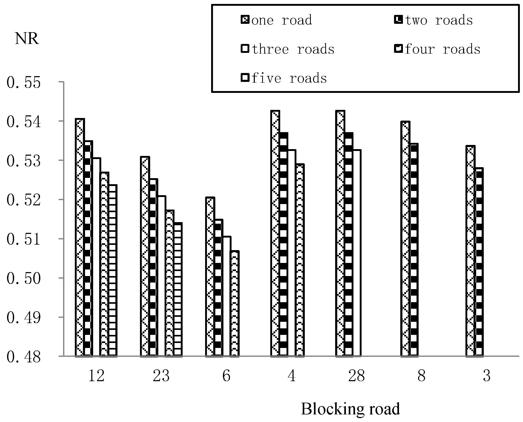
It was assumed that $v_i=90\mathrm{km}/\mathrm{h}$ and $v_{i,80}=60\mathrm{km}/\mathrm{h}$. The highway network of the researched region was as shown in Figure 2. It was assumed that one highway blockage occurred and that several highways were congested (assumed speed of 10 km/h); NR Equation (10) is shown in Table 4 and Figure 13.

Table 4. NR with a blockage or congestion on highways.

Blocked Highway	Congested Highway	Number of Low-Speed Highways	Travel Time Reliability	Connection Reliability	Network Reliability
12	13	1	0.9558	0.355	0.5405
	13, 14	2	0.9375	0.355	0.5349
	13, 14, 15	3	0.9234	0.355	0.5305
	13, 14, 15, 16	4	0.9116	0.355	0.5269
	13, 14, 15, 16, 17	5	0.9011	0.355	0.5236
23	22	1	0.9558	0.341	0.5308
	22, 24	2	0.9375	0.341	0.5252
	22, 24, 27	3	0.9234	0.341	0.5209
	22, 24, 27, 29	4	0.9116	0.341	0.5172
	22, 24, 27, 29, 31	5	0.9011	0.341	0.5140
6	7	1	0.9558	0.326	0.5205
	7, 4	2	0.9375	0.326	0.5148
	7, 4, 10	3	0.9234	0.326	0.5105
	7, 4, 10, 3	4	0.9116	0.326	0.5068
4	5	1	0.9558	0.358	0.5426
	5, 9	2	0.9375	0.358	0.5369
	5, 9, 2	3	0.9234	0.358	0.5326
	5, 9, 2, 3	4	0.9116	0.358	0.5289
28	23	1	0.9558	0.358	0.5426
	23, 29	2	0.9375	0.358	0.5369
	23, 29, 31	3	0.9234	0.358	0.5326
8	3	1	0.9558	0.354	0.5398
	3, 7	2	0.9375	0.354	0.5342
3	2	1	0.9558	0.345	0.5336
	2, 4	2	0.9375	0.345	0.5280

Figure 13. NR with a blockage or congestion on highways.

From Table 4 and Figure 13, the blocked highways 6, 12, and 23 caused a quick decline in NR. The three nodes had high node degrees of 8, 9, and 9, respectively. The blocked highways 3, 4, 8, and 28 had relatively low node degrees of 6, 4, 5, and 5, respectively. For the highways with a high node degree that connected well with other highways, their blockage affected many highways in the adjacent area and cause a rapid decline in NR. Therefore, much attention should be paid to these highway networks in traffic guidance or emergency response.

9. Conclusions

A new method calculating TTR based on the delay coefficient was proposed. The change rule of TTR was studied under different average speeds. Under the mixed conditions of highway blockage and highway congestion, the variation trend of highway NR using different methods was obtained. By comparing different TTR models, the proposed method had a similar change rule as the classified TTR models based on the same highway network in Jiangsu province, and the new method could be verified. It was practical to calculate a large-scale complex highway network and helpful. On the other hand, finding the important nodes and roads was helpful to improve the robustness of the network. Some detail conclusions are as follows:

(1) The new TTR method based on the delay coefficient was verified to be effective by comparison with the other methods. It can be used in the mixed scenario of blocked highways and congested highways.

(2) A highway blockage with a high node degree will seriously affect the whole highway network. Increasing the number of highways, especially highways with a high node degree, is an effective way to improve the CR of a highway network.

(3) For the large-scale highway network, the variation in TTR was analyzed under different travel time coefficients and different delay coefficients. The new model of TTR effectively reflected the network operation characteristics under different traffic conditions.

(4) With the increase in the number of congested highways, the TTR of the highway network decreased rapidly; with the increase in the travel time coefficient and delay coefficient, the TTR of the highway network had a tendency to decrease. Only when the travel time coefficient and delay coefficient took the minimum value did the TTR of the highway network demonstrate the maximum value.

(5) The number of low-speed highways, the average speed, and the 80% travel speed of highways were the most impact factors. The former factor was positively correlated with TTR, and the latter two factors were negatively correlated with TTR.

(6) By calculating the weighted TTR and connection reliability, the traffic reliability of a highway network can be comprehensively judged from both the network structure and operational status.

References

- Taylor, M.A.; Susilawati. Remoteness and accessibility in the vulnerability analysis of regional road networks. Transp. Res. Part A-Policy Pract. 2012, 46, 761–771. [Google Scholar] [CrossRef] [Scilit]
- Berdica, K. An introduction to road vulnerability: What has been done, is done and should be done. Transp. Policy 2002, 9, 117–127. [Google Scholar] [CrossRef] [Scilit]
- Snelder, M.; Van Zuylen, H.J.; Immers, L.H. A framework for robustness analysis of road networks for short term variations in supply. Transp. Res. Part A-Policy Pract. 2012, 46, 828–842. [Google Scholar] [CrossRef] [Scilit]
- Clark, S.; Watling, D. Modelling network travel time reliability under stochastic demand. Transp. Res. Part B 2005, 39, 119–140. [Google Scholar] [CrossRef] [Scilit]
- Carrion, C.; Levinson, D.M. Value of Travel Time Reliability: A Review of Current Evidence. Transp. Res. Part A-Policy Pract. 2012, 46, 720–741. [Google Scholar] [CrossRef] [Scilit]
- Rakha, H.; El-Shawarby, I.; Arafeh, M. Trip Travel-Time Reliability: Issues and Proposed Solutions. J. Intell. Transp. Syst. 2010, 14, 232–250. [Google Scholar] [CrossRef] [Scilit]
- Yang, S.; Wu, Y. Mixture Models for Fitting Freeway Travel Time Distributions and Measuring Travel Time Reliability. Transp. Res. Rec. 2016, 2594, 95–106. [Google Scholar] [CrossRef] [Scilit]
- Lu, C.; Dong, J. Estimating freeway travel time and its reliability using radar sensor data. Transp. B-Transp. Dyn. 2018, 6, 97–114. [Google Scholar] [CrossRef] [Scilit]
- Woodard, D.; Nogin, G.; Koch, P.; Racz, D.; Goldszmidt, M.; Horvitz, E. Predicting Travel Time Reliability using Mobile Phone GPS Data. Transp. Res. Part C-Emerg. Technol. 2017, 75, 30–44. [Google Scholar] [CrossRef] [Scilit]
- Wang, J.; Wang, C.; Lv, J.; Zhang, Z.; Li, C. Modeling Travel Time Reliability of Road Network Considering Connected Vehicle Guidance Characteristics Indexes. J. Adv. Transp. 2017, 2017, 2415312. [Google Scholar] [CrossRef] [Scilit]
- Guo, F.; Rakha, H.; Park, S. Multistate Model for Travel Time Reliability. Transp. Res. Rec. 2010, 2188, 46–54. [Google Scholar] [CrossRef] [Scilit]
- Bhouri, N.; Haj-Salem, H.; Kauppila, J. Isolated versus coordinated ramp metering: Field evaluation results of travel time reliability and traffic impact. Transp. Res. Part C-Emerg. Technol. 2013, 28, 155–167. [Google Scholar] [CrossRef] [Scilit]
- Sun, Y.; Shi, J.; Schonfeld, P.M. Identifying passenger flow characteristics and evaluating travel time reliability by visualizing AFC data: A case study of Shanghai Metro. Public Transp. 2016, 8, 341–363. [Google Scholar] [CrossRef] [Scilit]
- Uchida, K. Travel Time Reliability Estimation Model Using Observed Link Flows in a Road Network. Comput.-Aided Civ. Infrastruct. Eng. 2015, 30, 449–463. [Google Scholar] [CrossRef] [Scilit]
- Guo, Z.; Wang, W. Area traffic control system evaluation method based on travel time reliability. J. Southeast Univ. 2010, 40, 848–851. (In Chinese) [Google Scholar]
- Sun, C.; Cheng, L.; Zhu, S.; Han, F.; Chu, Z. Multi-criteria user equilibrium model considering travel time, travel time reliability and distance. Transp. Res. Part D-Transp. Environ. 2017, 66, 3–12. [Google Scholar] [CrossRef] [Scilit]
- Xu, L. Urban road Transportation Network Design Problem Based on Reliability Analysis. Ph. D. Thesis, Beijing Jiaotong University, Beijing, China, 2006. (In Chinese) [Google Scholar]
- Zhi, L.; Zhou, X.; Zhao, J. Vehicle Routing for Dynamic Road Network Based on Travel Time Reliability. IEEE Access 2020, 8, 190596–190604. [Google Scholar] [CrossRef] [Scilit]
- Chen, B.Y.; Li, Q.; Lam, W.H. Finding the k reliable shortest paths under travel time uncertainty. Transp. Res. Part B-Methodol. 2016, 94, 189–203. [Google Scholar] [CrossRef] [Scilit]
- Shams, K.; Asgari, H.; Jin, X. Valuation of travel time reliability in freight transportation: A review and meta-analysis of stated preference studies. Transp. Res. Part A Policy Pract. 2016, 102, 228–243. [Google Scholar] [CrossRef] [Scilit]
- Bai, X.H. Review on travel time reliability research of freeways. J. Transp. Eng. Inf. 2014, 12, 71–76. (In Chinese) [Google Scholar]
- Schroeder, B.J.; Rouphail, N.M.; Aghdashi, S. Deterministic Framework and Methodology for Evaluating Travel Time Reliability on Freeway Facilities. Transp. Res. Rec. 2018, 2396, 61–70. [Google Scholar] [CrossRef] [Scilit]
- LI, F.; Guo, R.J. The complex network characteristics of urban trunk road network. J. Shandong Univ. Technol. 2016, 30, 16–25. [Google Scholar] [CrossRef] [Scilit]
- Li, Q.; Zhou, G.J.; Zuo, R. Reliability analysis of highway network in China based on complex network theory. IOP Conf. Ser. Mater. Sci. Eng. 2020, 792, 012018. [Google Scholar] [CrossRef] [Scilit]
- Higatani, A.; Kitazawa, T.; Tanabe, J.; Suga, Y.; Sekhar, R.; Asakura, Y. Empirical analysis of travel time reliability measures in hanshin expressway network. J. Intell. Transp. Syst. 2009, 13, 28–38. [Google Scholar] [CrossRef] [Scilit]
- Higatani, A.; Kitwazawa, T.; Tanabe, J. Empirical analysis of travel time reliability measures in urban expressway network. Turk. J. Pediatr. 2007, 53, 522–527. [Google Scholar]
- Tang, X.Y. Travel time reliability assessment for traffic network. China Civ. Eng. J. 2007, 40, 84–88, 110. (In Chinese) [Google Scholar]
- Lomax, T.; Schrank, D.; Turner, S.; Margiotta, R. Selecting Travel Reliability Measures; NCHRP Draft Report; Texas Transportation Institute: Bryan, TX, USA, 2003. [Google Scholar]
- Sumalee, A.; Pan, T.; Zhong, R.; Uno, N.; Indra-Payoong, N. Dynamic stochastic journey time estimation and reliability analysis using stochastic cell transmission model: Algorithm and case studies. Transp. Res. Part C 2013, 35, 263–285. [Google Scholar] [CrossRef] [Scilit]
Publisher’s Note: MDPI stays neutral with regard to jurisdictional claims in published maps and institutional affiliations. |
© 2022 by the authors. Licensee MDPI, Basel, Switzerland. This article is an open access article distributed under the terms and conditions of the Creative Commons Attribution (CC BY) license (https://creativecommons.org/licenses/by/4.0/).