


Abstract
The integration of electric vehicles with grid vehicles promotes the creation of multi-energy microgrid models. One of the aims of these models is to decrease electricity usage through Vehicle-to-Grid planning. Effective management of microgrids necessitates sophisticated automation and control systems, which can prove challenging to establish and sustain. To tackle these challenges, the author introduces a hybrid model that merges a Linear Regression model and a Feedforward Neural Network, created using Matlab software. This combined algorithm adjusts the quantity of hidden neurons to enhance performance, guided by the evaluation criteria of Mean Squared Error, Root Mean Squared Error, and Mean Absolute Percentage Error based on batteries B0005, B0006, and B0007 from the NASA PCoE Research Center Dataset. The author forecasts the lifespan of the battery that most accurately reflects its degradation, revealing important implications for the future advancement of systems that employ Linear Regression and Feedforward Neural Networks for integrating electric vehicles into Vehicle-to-Grid systems. The comparison among the training, testing, and validation stages of the methodology serves to thoroughly demonstrate its effectiveness. Furthermore, the author indicates that the LR-FFN algorithm provides predictive tools relevant for the management of V2G-compatible EV systems and performs superiorly compared to other methods noted in the existing literature. Additionally, the author aimed to specifically identify the attributes of the LR-FNN model for prospective usages, emphasizing its efficacy in developing effective microgrid management, promoting energy efficiency, and ensuring that microgrids remain secure and resilient against failures or threats.
1. Introduction
Lithium-ion batteries have transformed various sectors owing to their impressive energy density, effectiveness, and adaptability. Notably, these batteries serve as the main energy source for electric vehicles (EVs) [1,2,3,4], powering a multitude of gadgets including smartphones, laptops, and tablets [5,6,7,8]. They are also utilized in large-scale energy storage solutions to accumulate surplus power from renewable sources like solar and wind energy [9,10,11,12]. Additionally, due to their compactness and reliability, these batteries are essential in numerous medical technologies, such as portable defibrillators and insulin pumps [13,14,15,16]. Vehicle-to-Grid (V2G) technology allows electric vehicles to act as portable energy storage systems, enabling them to both pull from and contribute energy to the grid. This capability can improve energy distribution, facilitate the incorporation of renewable energy, and offer backup power during peak demand or outages, thus aiding in grid balance while promoting effective energy utilization [17]. V2G systems represent cutting-edge innovation in scientific exploration, reshaping the methods of energy storage and consumption. This technology permits electric vehicles to not only receive energy but also to return it to the grid, effectively transforming them into mobile energy centers. For researchers globally, these systems embody a more robust and efficient energy framework. This creates an interactive dynamic where electric vehicles function as both energy consumers and suppliers, thereby aiding grid stability by storing excess power during low demand and releasing it during high demand. This dual functionality brings advantages for both efficiency and sustainability. Electric vehicles, along with their lithium-ion batteries, create an energy distribution system capable of stabilizing the grid, averting blackouts, and optimizing energy consumption. This positions vehicles as vital components of a smart energy network that redefines our approach to sustainable energy solutions [18]. Indeed, researchers are investigating diverse structures, control techniques, and associated services aimed at maximizing the effectiveness of electric vehicles in V2G contexts. This research includes refining how electric vehicles can deliver support services to the grid, such as balancing loads, reducing peaks, and transferring loads. More specifically, V2G technology aids in achieving a more balanced energy distribution across the grid, lowering the risk of overloads, providing energy during peak periods, thus minimizing the necessity for additional power generation units, and shifting energy usage to off-peak times, thereby enhancing the convenience of energy consumption. Particularly, Perez in his article [19] presents a thorough examination of the present status and future developments in Vehicle-to-Grid (V2G) technologies, underlining the critical importance of communication and data science to their efficacy. The article addresses increasing electricity demand, concerns regarding climate change, and the challenges involved in managing variable renewable energy sources. The authors illustrate how V2G strategies can mitigate these challenges by offering support services such as load balancing, peak reduction, and load transfer. Furthermore, the article outlines significant challenges faced in V2G implementation, including technical, regulatory, and economic obstacles, while exploring potential advantages and opportunities, such as enhanced grid stability and better integration of renewable energy sources [19]. Zhang in his article [20] evaluates the most recent developments in vehicle-to-grid (V2G) technology, concentrating on the control systems designed to manage the energy exchange between electric vehicles and the grid. He emphasizes the economic advantages of V2G, such as cost reductions for both EV owners and grid operators, along with possible income through energy transactions. Nevertheless, he also identifies considerable challenges that may surface, including technological difficulties, regulatory barriers, and financial limitations. The author concludes that while V2G provides numerous benefits, overcoming these difficulties is essential for broader acceptance [20]. Bortolotti, in his article [21], advocates for a comprehensive strategy regarding V2G integration, focusing on several elements, including energy demand, grid infrastructure, and regulatory policies. The authors stress the significance of integrated resource planning in enhancing V2G systems to ensure effective resource usage and reduced costs. They also outline the potential advantages of V2G systems, which include improved grid stability, enhanced integration of renewable energy sources, and decreased dependency on conventional power plants. The challenges in implementing V2G are described in the article, detailing technical issues, regulatory complications, and economic constraints. Furthermore, the article offers possible solutions to surmount these difficulties and discusses future research directions for V2G, encompassing advancements in communication technologies, data analysis, and regulatory frameworks. In summary, the article indicates that V2G technology has substantial potential to bolster both the efficiency and sustainability of the power grid, while also highlighting the critical collaboration among stakeholders necessary for its successful application [21]. Sassi [22] presents a summary of the current landscape and future prospects in Vehicle-to-Grid (V2G) and wireless V2G technologies. It elaborates on the capabilities of these technologies to establish user-friendly electricity markets and underscores the existing two-way wireless power transfer technology available for electric vehicles (EVs). The article also examines the challenges and opportunities involved in the implementation of V2G and wireless V2G systems, emphasizing the significance of improvements in communication protocols and power transfer efficiency [22]. Zountouridou, in his article [23], reviews several wireless access technologies vital for enabling Vehicle-to-Grid (V2G) applications. He outlines the critical role of wireless communication in facilitating effective and trustworthy V2G systems, where electric vehicles can connect with the power grid. In this work, various technologies such as Wi-Fi, Bluetooth, and Dedicated Short-Range Communications (DSRC) are evaluated based on parameters including data transfer speed, dependability, and security. The author also introduces new challenges such as interference and latency, offering solutions and suggestions for advancements to enhance V2G implementation [23]. The specific integration of vehicle-to-grid (V2G) frameworks with electric vehicles continues to present a current and compelling challenge, encouraging multiple approaches. Researchers are diligently examining solutions for new energy demand models designed to optimize the benefits and utilize lithium-ion batteries more effectively in V2G applications, devising advanced algorithms to predict energy demand, optimize battery charging and discharging, and improve the integration of renewable energy sources. Specifically, innovative models based on Machine Learning are being investigated to enhance V2G technology and achieve these significant objectives [24,25]. Naik, in his publication [24], highlights the capabilities of Vehicle-to-Grid (V2G) technology in enhancing the development of smart grids. His analysis reviews various investigations concerning the integration of electric vehicles (EVs) into the grid ecosystem. Furthermore, he suggests innovative solutions to tackle prospective challenges related to V2G advancements. The paper delves into optimization strategies for upgrading V2G functionalities, concentrating on advancements in network stability, cost reduction, and describing enhancements in overall performance achieved through sophisticated algorithms [24]. Du, in his article [25], investigates a machine learning-based, multi-objective optimization strategy for V2G systems that primarily relies on data-driven user demand responsiveness. His study assesses the applicability of machine learning algorithms in effectively forecasting and regulating energy consumption. Furthermore, this research emphasizes the charging characteristics of electric vehicles across various regions and delineates the energy storage management strategy connecting EVs with the grid through V2G. The findings underscore the advantages of this methodology, including enhanced grid stability, optimal resource utilization, and improved overall efficiency in V2G operations, as well as directions for future research [25]. According to another source [26], the batteries of EVs possess specific attributes that are not easily quantifiable directly. The indirect nature of measuring these battery-specific values introduces substantial challenges. Factors such as battery degradation, surrounding environmental conditions, internal temperature fluctuations, and material composition have an impact on performance; however, accurately assessing these in real-time is complicated. As a result, a significant number of researchers are focusing on advanced modeling and machine learning methodologies, which can yield predictive insights grounded in observable data [27]. To analyze these challenging-to-measure parameters, researchers have employed crucial data-driven techniques in their investigations and described the intricate workings of artificial neural networks (ANN) [28,29,30,31,32,33]. Chaturvedi, within a relevant work [34], evaluates an established electrochemical model sourced from the existing literature. The intent of the author is to present the recommended model through the lens of systems and controls while addressing the research obstacles inherent to the modeling, estimation, and regulation of lithium-ion batteries. Moreover, he introduces a new evaluation of various machine learning models, including ANN, aimed at studying lithium-ion batteries. The approach adopted for scrutinizing this reformulated model entails deriving an approximate model known as the single particle model, along with identifying its approximation limitations. EVs integrate with power grids, enabling bidirectional energy flow and can store and return surplus electricity to the grid. One feasible solution to increase the flexibility of the grid is the use of EV batteries, by storing surplus electricity and supplying it back when needed. The presence of bidirectional energy exchange is empowered by this process, allowing individuals and companies to contribute flexibility in electricity markets and helping to maintain the supply–demand balance [35]. The research work by Xiao [36] introduces an innovative event-based framework for frequency regulation in power systems that integrates the contribution of electric vehicles (EVs). The objective of the study is to enhance communication efficiency while improving the performance of secondary frequency control. Regarding the Event-Based Frequency Regulation Framework, the author proposes a strategy in which EVs participate in frequency regulation through vehicle-to-grid (V2G) functionalities. Unlike traditional approaches relying on continuous communication, the framework employs event-triggered signaling, which significantly reduces communication requirements. The model incorporates the charging and discharging behavior of distributed EV aggregators, along with realistic travel patterns, thus enabling a more accurate representation of EV impact on grid stability. In particular, the paper presents a new event-driven mechanism designed to optimize the transmission of control commands from dispatch centers to both generators and EV aggregators. This mechanism uses broadcast actions that adapt to real-time bandwidth availability, ensuring robust performance under varying network conditions. In doing so, it prevents communication congestion while maintaining effective control capability. Article [37] examines the challenges associated with the State of Charge (SOC) and State of Health (SOH) of batteries. To address these issues, the authors introduce a combined SOC/SOH co-monitoring framework capable of accounting for battery behavior in the presence of unknown but bounded preprocessing and measurement noise (UBB). The proposed approach incorporates the dynamics of two interdependent monitoring units and integrates measurements acquired on different time scales, which are updated intermittently. The framework determines measurement updates by considering both variations in the measured signals and the real-time conditions of the communication network, making efficient use of limited and time-varying resources. The actual SOC and SOH trajectories are continuously reconstructed through a pair of coupled monitors, developed using state predictors and estimators designed specifically for joint SOC/SOH assessment. To enhance system resilience, the authors propose an attack-detection strategy based on calculating the intersection over union (IoU), enabling the identification of potential malicious disturbances. Finally, a compensation mechanism is introduced to replace corrupted state estimates when an attack is detected, thereby mitigating its adverse effects. Jerouschek, in his research [38], addresses the complexities tied to the modeling, estimation, and management of lithium-ion batteries. He conducts an in-depth analysis of the model to predict battery behavior, assess state of charge (SoC), and realize effective control strategies. The investigation further explores the deployment of machine learning methodologies, notably artificial neural networks (ANN) [39,40,41,42,43], to enhance the precision and efficacy of these systems. Many scholars have frequently combined the Linear Regression (LR) model with Artificial Neural Networks (ANN) in their studies. The LR model offers several advantages when paired with ANN for predicting the State of Health (SOH) and Remaining Useful Life of lithium-ion batteries. The benefits of integrating linear regression (LR) with artificial neural networks (ANN) in the examination of lithium-ion batteries are extensive. The first advantage is cross-validation; LR can function as a straightforward reference model to validate the reliability and robustness of more complex models such as ANNs. The second advantage is interpretability; LR provides clear insights into the relationships between independent and dependent variables, facilitating the identification of critical factors affecting battery performance. The third benefit is training speed; LR typically requires less computational time for training compared to ANNs, enabling quicker iterations and initial analyses. In addition, LR is less prone to overfitting, particularly when dealing with noisy or limited datasets, thereby serving as a foundation for understanding the intricate nature of the data. Feedforward Neural Networks (FNNs) represent one fundamental category of artificial neural networks (ANNs). In FNNs, data progresses through neurons in a singular direction, from input to output, devoid of loops or feedback. These networks are applied in a variety of tasks, including classification and regression. The combined utilization of both models—LR for linear trends and FNN for complex nonlinear trends—provides predictive tools relevant for the management of V2G-compatible EV systems and facilitates a more robust and precise analysis of lithium-ion batteries. The fusion of Linear Regression (LR) with Feedforward Neural Networks (FNN) offers a powerful methodological framework. Researchers utilize LR due to its straightforwardness and interpretability, which aid in understanding fundamental relationships within the dataset. Subsequently, FNN is employed to capture complex nonlinear patterns that may not be addressed by the linear dimensions of LR. This synergistic approach augments predictive accuracy and fosters a more comprehensive understanding of the data. The objective of this research is to examine the integration of electric vehicles (EVs) with vehicle-to-grid (V2G) technology along with the factors influencing lithium battery condition in order to develop a model that assesses the life condition of a battery. The primary goal of this article is to establish a predictive model for determining the aging condition of lithium batteries by employing both LR and FNN models. Cervellieri presents an innovative method for selecting model architecture aimed at defining an optimal mixed configuration, grounded on comparisons with known techniques and the minimization of errors, specifically MSE (Mean Squared Error), RMSE (Root Mean Squared Error), MAPE (Mean Absolute Percentage Error), and RMSPE (Root Mean Squared Percentage Error) for battery models B0005, B0006, and B0007 [44,45] sourced from the NASA PCoE Research Center dataset.
This article is structured in the following manner:
- Section 2 presents an overview of the Data Acquisition NASA Prognostics Center of Excellence Dataset;
- Section 3 outlines the development of the LR-FNN Model and its architectural framework;
- Section 4 details the proposed methodology for the LR-FNN;
- Section 5 examises the Mathematical Formulas
- Section 6 examines the results along with discussions;
- Section 7 provides Comparison between the proposed Hybrid Algorithm and other Methods in the Literature;
- Section 8 provides the Concept of Robustness
- Section 9 examines the Generalization
- Finally, Section 10 summarizes the conclusions.
2. Describes the Data Acquisition NASA Prognostics Center of Excellence Dataset
This section provides an overview of the Feed-Forward Neural Network (FNN) propagation system related to the Linear Regression network utilizing the NASA Prognostic Center of Excellence dataset [1]. Specifically, the predicted lifespan of batteries is assessed through the repeated processes of charging and discharging. Experimental development data from NASA’s PCoE Research Center supports the mixed algorithm I developed. The batteries B0005, B0006, and B0007 undergo thorough and simultaneous charge and discharge cycles based on predetermined parameters and environmental conditions linked to the completed charge and usage metrics from the environmental chamber. The researchers opted to investigate the internal characteristics of the batteries by conducting periodic measurements of the Electrochemical Impedance Spectroscopy (EIS) parameters. In this paper, a hybrid algorithm was formulated, integrating advanced FNN and LR models, and was evaluated using experimental data from NASA’s PCoE Research Center, including test duration, passage time, cell surface voltage, and temperature. The researchers carried out simulation tests by extracting available data from the official NASA PCoE Research Center website.
As illustrated in Figure 1, Figure 2 and Figure 3, the parameters of current, voltage, and temperature for batteries B00005, B00006, and B00007 exhibit significant variations during charge or discharge phases as they age. During charging, for instance, the current transitions from 1.5 A to 0 A in the initial phase and reaches 0.2 A at 5500 s, while in the discharge process, the current starts at −2 A and concludes at 0 A. The associated voltage during charging for battery B0005 starts from an initial value of 3.8730 V and rises to a final value of 4.1911 V. Figure 1 depicts the capacity trend during discharge, beginning at 1.8564 and ending at 1.3250. For battery B0006, during charging, the initial current reads 8.1999 A with a starting voltage of 3.8646 V until it hits the voltage limit of 4.2 V. The discharge for battery B0006 initiates with a current of −2 A, reaching a voltage limit of 2.6 V. Figure 2 illustrates the capacity trend during discharge ranging from an initial value of 2.0353 to a final value of 1.1856. Figure 3 demonstrates the capacity trend during discharge from an initial value of 1.8910 to a final value of 1.4324.
Figure 1.
Trend of Capacity in case of discharge for battery B0005. The discharge capacity of battery B0005 shows a steady decline over successive cycles, consistent with typical battery aging behavior.
Figure 2.
Trend of Capacity in case of discharge for battery B0006. For battery B0006 under rapid-discharge conditions, capacity decreases progressively with cycling. The degradation is initially mild but accelerates after the knee point, likely due to combined mechanisms such as SEI layer growth, lithium plating, and electrode structural deterioration.
Figure 3.
Trend of Capacity in case of discharge for battery B0007. Battery B0007 exhibits a gradual reduction in discharge capacity across repeated charge–discharge cycles, a process commonly referred to as capacity fade. Although the overall decline is approximately monotonic, minor fluctuations may appear due to transient recovery effects or measurement variability.
3. Described the LR-FNN Model Development and the Architecture of the Model
The estimation of State of Health (SOH) and the assessment of Remaining Useful Life (RUL) have been accomplished through a hybrid algorithm integrating Linear Regression and Feedforward Neural Network techniques. The results achieved, along with the computed errors, demonstrate a high level of precision in estimating the SOH. Three specific parameters were selected—discharge capacity, cycle number for current integral, and cycle number—based on their relevance in predicting the State of Charge SOH.
The model was trained using 80% of the available dataset, while 10% was reserved for the testing phase and the remaining 10% was allocated to validation.
This partitioning was guided by evaluations focusing on the characteristics of the hybrid algorithm developed to ensure the reliability of the outcomes. The “poslin” activation function was applied in this study, situated between the input and hidden layers, which is illustrated in Equation (1):
f(x) = max(0,x)
This implies that for a positive input x, the output corresponds to x; if the input is negative, the output becomes 0. The non-linearity brought by the ReLU function enhances the ability of neural networks to learn intricate patterns and supports a computation-efficient process. The author opted for a Linear activation function in the output layer, described in Equation (2):
The integration of Linear Regression (LR) with Feedforward Neural Networks (FNN) led to the development of strong models for SOH prediction. The hybrid algorithm commenced by analyzing data using LR to establish the necessary features for both input and output parameters, enabling the recognition of SOH trends. Initiating the process with LR aids in understanding the fundamental linear relationships present in the data from the NASA PCoE Research Center. Logistic regression is primarily used to obtain a preliminary representation of data characteristics, ensuring that the most relevant information is available to the latent reasoning module of the LLM-based model. This approach yields a straightforward and interpretable model capable of emphasizing significant predictors. Insights derived from the LR model were utilized to generate new features that encapsulate critical trends and correlations within the data. For the training segment, the FNN model was employed, incorporating the parameters obtained from the earlier analysis into a Feedforward Neural Network. This method is essential as FNN can recognize more intricate, non-linear patterns that LR potentially overlooks. An Ensemble Approach was utilized, merging predictions from both the LR and FNN models to enhance overall accuracy. This hybrid method effectively combines the simplicity and interpretability of LR with the advanced pattern recognition capabilities of FNN, rendering it a flexible strategy for optimizing model performance, see the diagram of hybrid algorithm of Linear Regression (LR) and Feedforward Neural Network (FNN) (Figure 4).
f(x) = x
Figure 4.
Diagram of the hybrid algorithm of Linear Regression (LR) and Feedforward Neural Network (FNN).
4. Described the Proposed LR-FNN Methodology
The software outlined within the MATLAB 2025 script is crafted for the purpose of examining battery cycle data to forecast the State of Health (SOH) and determine the degradation of batteries. It utilizes a combination of a Linear Regression model and a Feedforward Neural Network (FNN) for making these estimations. The predictive framework adopts a cascade structure: Logistic Regression (LR) generates a first representation of the characteristics starting from the input data, which is subsequently used by the Feedforward Neural Network (FNN) to model higher order non-linear interactions. This sequential application helps to improve both the interpretability and the overall performance of the model. The following hybrid algorithm is structured into several distinct phases. In the Battery Data Selection phase, the user indicates the specific battery data file to be loaded. The script accommodates multiple datasets, each recognized by unique identifiers (B0005, B0006, and B0007). During the Data Loading phase, the chosen battery data file is incorporated into the MATLAB environment. In the Variable Assignment phase, the information from the file is designated to a variable for more straightforward access. Regarding data analysis, the initial phase is Cycle Range Specification, where the script establishes the cycle range for analysis, usually starting from the second cycle and concluding at the second-to-last cycle. The second phase is Capacity Calculation, which consists of two processes. The first process is the Discharge Capacity Calculation, where the script computes the discharge capacity by integrating the current recorded during each discharge cycle. The second process involves Extraction from Dataset, wherein direct discharge capacity values are retrieved from the dataset for comparison and additional scrutiny. In the SOH prediction phase, two procedures are executed. The first is the SOH Calculation, which determines the SOH as the ratio of discharge capacity at each cycle to the rated capacity. The second procedure, Feature Preparation, involves organizing features for the prediction models, including discharge capacity and cycle number. In the Modeling and Prediction phase, an interaction is established between the Linear Regression algorithm and the Feedforward Neural Network. The first algorithm is employed for Model Training and SOH Prediction, while the second algorithm focuses on defining activation functions, network training, and SOH forecasting. Specifically, in the Linear Regression algorithm, a model is prepared using the features and the calculated SOH. The SOH prediction is executed via the trained linear regression model. Moreover, for the Feedforward Neural Network (FNN) algorithm, the FNN is configured with designated numbers of inputs, hidden layers, and hidden units. The activation functions for the network layers are also outlined. Furthermore, the dataset is partitioned into training, validation, and testing subsets, and the FNN is trained with the organized features and SOH values. The SOH is predicted through the trained FNN. To assess the performance, various metrics are defined to gauge the accuracy and reliability of the proposed hybrid algorithm. In evaluating metrics such as Mean Squared Error (MSE), Root Mean Squared Error (RMSE), Mean Absolute Percentage Error (MAPE), and Root Mean Squared Percentage Error (RMSPE) for batteries B0005, B0006, and B0007 from the NASA PCoE Research Center dataset, the hybrid model’s performance is appraised for its precision. In this study, LR was not used as the final predictive model; rather, it served as a methodological instrument for generating intermediate representations and informative feature sets. LR provides a straightforward and interpretable mechanism for capturing linear structures within the raw data, thereby facilitating subsequent processing by the Latent Reasoning modules within the LLM-based architecture. Within the overall computational pipeline, LR functions as an initial stage for producing meaningful and architecture-compatible features, contributing to dimensionality reduction and the identification of the most salient signals. Thus, LR does not constitute the central component of the final model; instead, it supports the data-preparation process, enabling the latent reasoning component to operate with greater stability and efficiency. The use of LR offers several methodological advantages:
- Establishing interpretable baseline representations for key features.
- Enhancing the stability of downstream training processes by providing inputs that are already filtered and information-rich.
- Increasing the transparency of the model’s early decision-making steps, thereby supporting ablation studies and clarifying why certain features exert a more pronounced influence on the final outcomes.
4.1. Parameters Considered for the Realization of the Model
The input parameters used in this study were obtained from the NASA dataset corresponding to battery B0005. The available variables include test_time (s), step_time (s), step_index, voltage (V), current (A), and surface_temperature (°C). These experimental data, provided by the NASA PCoE Research Center, form the basis for the simulations conducted in this work. The analysis focuses on using information from the charging phase to estimate the state of health (SOH) of battery B0005. To build and evaluate the predictive model, the dataset was divided into three parts: 80% for training, 10% for testing, and 10% for validation. This structure ensured that the model was developed, tuned, and assessed in a systematic and reliable manner. Overall, the modeling approach follows a sequential workflow, with each phase contributing to the refinement and verification of the final predictive framework. During the initial training stage, the model checks whether all the necessary conditions are satisfied. If they are, it moves on to the testing phase, where its performance is evaluated using the test dataset. If the criteria are not met, the process loops back to the beginning for further refinement. After completing the testing phase, the researcher finalized the development of the model and carried out its validation.
4.2. Normalization Techniques
Normalization plays an essential role in enhancing a model’s performance. It ensures that all features are expressed on a similar scale, preventing those with larger numerical ranges from disproportionately influencing the model’s behavior.
4.2.1. Min–Max Scaling
Min–Max Scaling helps bring all feature values into the same preset interval, usually between 0 and 1. This approach is particularly useful when the dataset includes variables expressed in different units or showing wide differences in their value ranges. The transformation is calculated using the formula:
- X is the original value of the feature;
- Xmin is the minimum value of the feature;
- Xmax is the maximum value of the characteristic;
- Xnorm is the normalized value.
4.2.2. Z-Score Normalization
Z-score normalization, often called standardization, reworks the data so that each variable has a mean of 0 and a standard deviation of 1. This method is especially useful when you want to compare characteristics by looking at how much each value deviates from its mean, measured in standard deviations.
The formula used is:
- X is the original value of the feature.
- µ is the average of the feature.
- σ is the standard deviation of the feature.
- X_std is the standardized value.
4.2.3. Hybrid Normalization Technique for the Calculation of the State of Health (SOH)
In this study, I tested both normalization methods on the dataset and compared their outcomes to identify which one delivered the best performance for the neural network. The results showed that z-score normalization led to a noticeable improvement compared to Min–Max Scaling. For this reason, when estimating the State of Health (SOH) of lithium-ion batteries, I adopted a hybrid normalization approach that draws from both Min–Max Scaling and z-score normalization. The code used for SOH calculation implements this combined strategy, merging elements of each technique to produce a more effective normalization tailored to the model’s needs.
SOH = capacity/initial_capacity;
4.2.4. Direct Model or Single Output Model
Figure 4 shows a single output model explained with the preprocessed dataset. The author chose to use three parameters as initial variables and a single element as the target variable. The State of Charge was chosen as the target and the output variable. The determined input variables are:
- X is the set of input variables;
- x1 is the battery current;
- x2 is the battery voltage;
- x3 is the battery temperature.
Similarly, the set of output variables can be represented as:
Figure 4 shows that there is only one output variable:
is the set of the output variables.
x ∈ R and y ∈ Rn.
Here, it is possible to define R as a real number.
4.2.5. Test Data and Training
The author illustrates in Figure 4 the structure of the Feed-Forward Back-Propagation Neural Network and displays three components in the input: the current, voltage, and temperature of battery B0005. For the discharge scenario, the output selected was the State of Health (SOH) value. The first hidden layer consisted of five neurons, while the second hidden layer also contained five neurons. As indicated in the following figures, three input variables were utilized, resulting in an input variable size of 3. The model was assessed using mean squared error and root mean squared error.
4.2.6. Training Algorithm Used
When the algorithm comes to the weights of the interconnection of the neurons in training, this was randomly initialized by its author. This trained data is fed into the network, from input to output and in this step, I calculated the difference between predicted output and required (desired) output.
After the training model is completed, 10% of data were used to validation the trained model.
At a certain level of desired accuracy, the algorithm is validated on new (10% of the dataset) data. The end result was that the researcher received highly accurate modeling results from simulations with R2 values approaching 1.0. In Figure 4, the proposed network consists of three layers with a total of three inputs for two hidden layers and an output layer.
The author has formulated a visualization of the Sigmoid function (Tansig), which is evident in the graph and is utilized within the hidden layer. Additionally, there is a depiction of the linear function (Purelin), which is applied in the output layer. To maintain transparency and guarantee the replicability of the reported scientific findings, Table 1 and Table 2 display the standard parameters for training the neural networks discussed in this study.
Table 1.
Parameters of Lithium-ion Batteries B0005, B0006, and B0007.
Table 2.
Assessment of standard parameters for neural network training.
5. Mathematical Formulas
The mathematical formulas of the hybrid algorithm can be classified as follows:
5.1. Prediction Models
5.1.1. Linear Regression
The linear regression model can be represented as:
Y = β0 + β1X1 + β2 X2 + …+ βp Xπ + ε
In which:
- Y is the dependent variable (State of Health—SOH);
- X1, X2, …, Xp are the independent variables;
- β0, β1, …, βp are the model coefficients;
- ε is the error.
5.1.2. Feedforward Neural Network
For a Feedforward Neural Network, a neuron’s output Y was calculated as:
In which:
- are the weights;
- are the input;
- b is the bias;
- f is the activation function.
5.1.3. Weight Update Rule
- wij: Weight between neurons (i) and (j);
- : Learning rate;
- : Error.
In the newly developed algorithm, the author has established a novel Equation (7) intended for calculating the weight between neurons (i) and (j). This equation incorporates a process of retroactive weight adjustment that is closely linked to both the Learning Rate and the errors generated by the output calculation algorithm. Through this innovative Equation (5), the author aims to facilitate an automated adjustment of neurons, allowing them to promptly adapt to retroactive trends that align with the Learning Rate, while also considering the errors produced by the hybrid algorithm [2]. The outcomes derived from this approach indicate that the model demonstrates enhanced performance and improved accuracy, distinguishing it as more favorable than traditional methodologies when evaluated against the existing literature. Equation (7) does not describe a simple standard update of the weights, as occurs in traditional gradient descent. On the contrary, it introduces a feedback mechanism that transfers the weights derived from the LR model within the FNN. In practice, the coefficients of the logistic regression are reworked through a fuzzy adaptation mechanism, so as to incorporate preliminary linear knowledge directly into the activation function of the neural network. This allows the FNN to maintain the ability to learn nonlinear relationships while benefiting from informed initialization. The novelty does not lie so much in the single formula, but in the synergistic combination between two components:
- LR component, which offers stability and interpretability, providing initial weights based on linear structures present in the data.
- FNN component, which acquires the residual non-linear relationships by updating the weights via a fuzzy mechanism that uses the weights coming from the LR model as a reference.
This integration allows a retroactive alignment of the weights: each update of the neural network is influenced by the underlying linear structure, favoring a more stable convergence and reducing uncertainty in learning.
The equation is designed to:
- Transfer information from the LR model to subsequent neural levels;
- Make the network more robust against noisy or incomplete data;
- Preserve a certain degree of interpretability on relevant parameters.
Although hybrid models exist in the literature (e.g., FNN GPR for battery health or KNN LR/LGB+LR approaches), these methods generally do not formalize an explicit transfer of linear weights within the activation of the neural network. My proposal instead introduces explicit and structured feedback, which represents the distinctive element of the method. I believe that these clarifications highlight the real innovative scope of the methodology: it is not a simple update of the weights, but a coherent integration of linear information into the fuzzy dynamics of the FNN, with measurable benefits in terms of stability, partial interpretability and adaptive capacity.
5.1.4. Mathematical Models of V2G Operations
- 1.
- SOC (State of Charge)
It is now defined as the amount of electrical charge currently available in the battery relative to its nominal capacity, expressed as a percentage. This parameter reflects the immediately usable charge level. In the revised text, I have clearly separated the definition of SOC and its estimation methodologies—such as coulomb counting, voltage-based approaches, and Kalman-filter-based techniques—from the discussion on mechanisms of battery degradation.
- 2.
- SOH (State of Health)
The manuscript now explicitly presents SOH as an indicator of the overall degradation of the battery with respect to its initial condition. This metric encompasses factors such as remaining capacity, internal resistance, and power capability, also expressed as a percentage. I have emphasized its conceptual distinction from SOC in order to prevent ambiguity between a battery’s instantaneous charge level and its long-term aging state.
- 3.
- RUL (Remaining Useful Life)
RUL is introduced as an estimate of the residual service life of the battery, derived from the combined analysis of SOC, SOH, and historical operating parameters. The revised text highlights more explicitly that RUL predictions are influenced by the degradation trends captured by the SOH metric.
- 4.
- State of Discharge
The manuscript clarifies the relationship between SOC and Depth of Discharge (DoD), where DoD represents the percentage of the battery’s capacity that has already been utilized. This relationship is expressed as:
For example, a battery with an SOC of 70% corresponds to a DoD of 30%, meaning that 30% of its total capacity has been consumed.
5.1.5. Charging and Discharging Optimization
The operational foundation of Vehicle-to-Grid (V2G) systems lies in the coordinated optimization of electric vehicle (EV) charging and discharging activities. This requires simultaneously ensuring the stability of the electrical grid, safeguarding battery health, and minimizing operational costs. To capture these interacting factors, the literature commonly adopts mathematical frameworks based on multi-objective optimization, defined over a time horizon and involving a fleet of vehicles.
Objective Functions may include:
- 1.
- Minimizing user charging/discharging cost:
- 2.
- Minimizing charging station waiting time:
- 3.
- Maximizing SOC at departure:
Constraints Include:
- Battery SOC limits:
- Power limits:
- Grid capacity constraints:
- EV availability windows: .
5.1.6. Dispatchable Capacity Modeling
The dispatchable capacity of each electric vehicle—namely, the portion of stored energy that can be made available to the grid without compromising the vehicle’s ability to meet its subsequent mobility requirements—is commonly defined as follows:
where:
- = battery capacity;
- = currentSOC;
- = minimum allowableSOC;
- = vehicle range per full charge;
- = expected travel distance to station .
This formulation expresses the available capacity as a function of the battery’s state of charge, anticipated travel needs, and planned discharge activities, thereby enabling more realistic and operationally coherent scheduling across multi-vehicle and multi-station V2G environments.
5.1.7. Frequency Regulation and Microgrid Stability
V2G participation can contribute to microgrid frequency stabilization by adjusting active power output in response to observed deviations.
where is again coefficient, is nominal frequency, and is the instantaneous gridfrequency.
In this study, the author presents a two-stage hybrid framework for estimating battery State of Health (SOH), which integrates regularized linear regression with a compact feedforward neural network. The innovative contribution does not lie merely in the combination of two modeling approaches, but rather in the conditional and modular structure adopted. In this formulation, the linear regression model provides an interpretable, low-variance baseline estimate, whereas the neural network is specifically trained to learn only the nonlinear residual relative to this baseline. The final prediction is then obtained as the sum of these two components.
where X_aug includes normalized features and concatenated LR estimation.
5.1.8. Algorithmic Architecture and Pipeline
This architecture makes it possible to leverage the respective strengths of both methods: the interpretability and stability offered by linear regression, and the capacity of the neural network to capture nonlinear relationships. The proposed approach is conceived to deliver higher accuracy, improved generalization in out-of-deployment conditions, and computational efficiency compatible with real-time implementation in battery management systems (BMS).
5.1.9. Feature Extraction and Pre-Processing
For each cycle or time interval, a set of physically meaningful features is extracted, including measured capacitance, estimated internal resistance R0, slope of the voltage–SOC curve, delivered energy, average current, discharge duration, temperature, and local degradation indicators. These features are then normalized using the μ and σ parameters computed on the training set:
X_norm = (X − μ)/σ.
Normalization is essential for ensuring the stability of both the regression process and the training of the FNN, as well as for enabling consistent and reproducible deployment within battery management systems (BMS).
5.1.10. Stage 1—Regularized Linear Regression (LR)
I estimate the parameter vector by minimizing the quadratic loss function augmented with an L2 regularization term (ridge regression).
The parameter vector is obtained as
The linear regression model then yields:
The regularization parameter is selected through cross-validation (either k-fold or leave-one-cell-out) to achieve an appropriate balance between bias and variance. The coefficients of the linear regression are further accompanied by estimates of their uncertainty (for example, via bootstrap confidence intervals), thereby enhancing their physical interpretability.
1. Construction of the Input for the FNN
Within the training set, the residual is first computed as
The input matrix for the feed-forward neural network (FNN) is then assembled by concatenating the normalized predictors, the linear regression predictions, and—where appropriate—additional nonlinear transformations (such as quadratic terms , interaction features, or sinusoidal functions of the cycle index to capture periodic patterns). Formally,
Incorporating into the input explicitly conditions the FNN to concentrate on correcting the residual bias left by the linear model, rather than attempting to reconstruct the entire input–output mapping from scratch. This design improves learning efficiency and enhances interpretability of the combined model.
5.1.11. Stage 2—FNN for Residual Modeling
The feed-forward neural network (FNN) is designed to remain deliberately compact—for example, comprising two hidden layers with approximately 50 neurons each and ReLU activation functions. The network is trained to predict the residual r through minimization of a loss function combining mean squared error (MSE) with an weight-decay regularization term applied to the network parameters.
Optimization is performed using the Adam algorithm, employing mini-batch learning and incorporating early stopping based on validation performance. Both the architectural hyperparameters and the early-stopping criteria are selected through systematic exploration, such as grid search or Bayesian optimization, conducted on the validation folds. Since the FNN is tasked exclusively with learning the residual component rather than the full input–output relationship, a model with substantially reduced capacity can be employed. This approach mitigates the risk of overfitting and lowers computational demands compared to a standalone FNN trained directly on the original targets.
Technical Motivation and Advantages Compared to Existing Methods.
5.1.12. Bias and Variance Reduction
The linear regression (LR) component captures the dominant linear relationships, which are generally transferable across different operating conditions. The feedforward neural network (FNN) is dedicated to modeling only the nonlinear residual component. Training the FNN on the residual reduces the network’s required complexity and increases its robustness to unseen data, yielding better performance than a standalone FNN.
5.1.13. Interpretability
The LR coefficients retain clear physical and statistical meaning, allowing the identification of the variables that most strongly influence the State of Health (SOH). This enhances the model’s acceptance in engineering contexts and supports diagnostic analyses aimed at understanding degradation mechanisms.
5.1.14. Robustness in Transfer Scenarios
In scenarios involving transfer across different conditions—such as varying currents, temperatures, or cell chemistries—the baseline linear estimate tends to generalize effectively. The FNN provides localized corrections without replacing the interpretable LR foundation, thereby improving performance under out-of-distribution conditions.
5.1.15. Efficiency and Deployability
The combined LR+FNN architecture reduces the overall computational burden compared with larger end-to-end neural networks. This efficiency is particularly important for deployment in Battery Management Systems (BMS), where computational and memory resources are limited.
5.1.16. Ease of Experimental Validation
The modular architecture enables clear ablation studies and systematic comparisons with alternative models, including LR-only, standalone FNN, Kalman filters based on electrical models, and standard machine learning approaches such as Support Vector Regression and Random Forest. Evaluation metrics include , , , and , as well as robustness assessments across test sets characterized by diverse operating conditions.
5.2. Model Evaluation
The author conducted a comparison between the performance of the hybrid model and that of separate LR and FNN models. The algorithm’s accuracy was measured using metrics that include the Evaluation of MSE (Mean Squared Error), RMSE (Root Mean Squared Error), MAPE (Mean Absolute Percentage Error), and RMSPE (Root Mean Squared Error) calculations for batteries B0005, B0006, and B0007 from the NASA PCoE Research Center dataset. This approach enabled the integration of the strengths inherent in both models, leading to enhanced precision and the robustness of the forecasts.
5.3. Training Algorithm
The training methodology implemented in the software aimed at the feedforward neural network (FNN) model adheres to a sequence of procedures designed to educate the model in forecasting the State of Health (SOH) of batteries. Initially, during the data preparation stage, the inputs for the neural network comprise significant features such as discharge capacity and cycle count. This information is structured into an array (X). Subsequently, the author identified a target variable—the State of Health (SOH)—which is organized into a vector (Y). The next stage involves configuring the neural network itself. The architecture includes an input layer, two hidden layers, and an output layer. Each hidden layer is specified to contain a predetermined number of units (neurons), with the author opting for two hidden layers, each consisting of 50 neurons. Concerning the activation functions, the ReLU (Rectified Linear Unit) activation function was selected for the hidden layers to incorporate nonlinearities. Conversely, a linear activation function was employed for the output layer to facilitate the model’s output. The dataset is partitioned into three subsets: the Training Set, which is devoted to training the model (utilizing 80% of the data); the Validation Set, which is utilized to fine-tune the model architecture and avert overfitting (utilizing 10% of the data); and the Test Set, which is engaged to assess the trained model’s performance (utilizing 10% of the data). When determining the training parameters, a specific parameter was selected that defines the magnitude of the incremental adjustments to be made when modifying the weights (Learning Rate), set at a value of 0.01. The training process is capped at a maximum of 1000 iterations (epochs). During the model training phase, the author employed an optimization algorithm to reduce the discrepancy between the model’s predictions and the actual SOH values. In the backward pass, the error is communicated backward through the network, resulting in updates to the weights and biases informed by the error gradient. Weights within the network are adjusted iteratively utilizing gradient descent to minimize the loss function, such as mean squared error. Throughout the training process, the model’s performance is evaluated on the validation set to guard against overfitting and to ascertain the appropriate moment to cease training. After training is concluded, the model undergoes evaluation using the test set to verify its competence in generalizing to novel data. Ultimately, the trained model is employed to predict the SOH of the input data, thereby offering insights into battery health.
6. The Results and Discussions
The author utilized the NASA dataset for batteries B0005, B0006, and B0007 in order to validate and test the hybrid algorithm. The training, testing, and validation stages are depicted in the following Figure 5, Figure 6 and Figure 7, represented as R2 plots corresponding to the three distinct phases during training for the anticipated cells. The author confirmed the validity of the algorithm after training the neural network by utilizing accessible data from NASA, leading to the development of a hybrid algorithm capable of yielding outputs with R2 values nearing 1. The results acquired were deemed satisfactory.
Figure 5.
Neural Network Training Regression B0005.
Figure 6.
Neural Network Training Regression B0006.
Figure 7.
Neural Network Training Regression B0007.
6.1. Performance Evaluation Metrics
In this paper, the author has assessed the efficacy of each phase—Training, Validation, and Testing—by employing the Mean Square Error (MSE) Formula (20) [44]:
where are defined:
- ○
- MSE is the Mean of error squares;
- ○
- Oa is Actual output;
- ○
- Op is Predicted output;
- ○
- n is the number of samples.
The MSE is characterized as the average squared difference between the predicted State of Health (SOH) values and the actual SOH values. The graphs illustrate that lower MSE values are indicative of superior algorithm performance. Notably, the optimal validation performance trends for the Mean Squared Error (MSE) concerning the batteries B0005, B0006, and B0007 from the NASA Prognostics Center of Excellence dataset are depicted in Figure 8, Figure 9 and Figure 10. These figures illustrate the performance trends across the Training, Validation, and Testing phases in relation to the epochs for the battery datasets of B0005, B0006, and B0007. For battery B0005, the Validation trend indicates a peak performance of 2.98110 × 10⁻⁵ at the 14th epoch. Battery B0006 exhibits a validation trend with an optimal performance of 2.404810 × 10⁻⁶ at the 7th epoch, while battery B0007 achieves a best performance of 4.095210 × 10⁻⁶ at the 7th epoch. In Figure 8, Figure 9 and Figure 10 the green circle indicates the best validation performance of 2.7548 × 10⁻⁷ at epoch 13 for battery B0005, the best validation performance of 1.1144 × 10⁻⁵ at epoch 6 for battery B0006, and the best validation performance of 1.0151 × 10⁻⁵ at epoch 2 for battery B0007.
Figure 8.
Best Validation Performance for battery B0005.
Figure 9.
Best Validation Performance for battery B0006.
Figure 10.
Best Validation Performance for battery B0007.
6.2. Evaluation Criteria—Root Mean Squared Error—Mean Absolute Percentage Error
In this study, the author has computed the Root Mean Squared Error (RMSE) and the Mean Absolute Percentage Error (MAPE) to assess the precision of the proposed hybrid algorithm for SOH prediction [44,45,46].
where:
- = actual value;
- = predicted value;
- n is the total number of observations.
- n is the total number of observations;
- y is the observed value;
- = predicted value by the model.
6.3. Prediction of SOH Results
In this study, following the computation of the Actual State of Health (SOH) using a combination of Linear Regression and Forward Neural Network models, these results were employed to estimate the SOH value at the final time point. The equation applied for determining the battery SOH is as follows (23):
In this paper, the author defines SOH as the ratio of the battery’s effective capacity (Ca) to its rated capacity (Cr), where effective capacity indicates the quantity of capacity actually utilized when the battery is fully charged. The rated capacity of a fully charged battery is represented as 100%, whereas the capacity of a fully depleted battery is 0%. The subsequent Figure 11, Figure 12 and Figure 13 illustrate the error trends during the Training, Validation, and Test phases for batteries B0005, B0006, and B0007, which were analyzed at the NASA PCoE Research Center. For battery B0005, the maximum error recorded is 0.1328 × 10⁻⁶. For battery B0006, the largest error noted is 0.9297 × 10⁻⁶. Battery B0007 has a maximum error of 0.3681 × 10⁻⁶. These findings affirm the effectiveness of the hybrid LR-FNN algorithm across all conducted simulations.
Figure 11.
Errors battery B0005.
Figure 12.
Errors battery B0006.
Figure 13.
Errors battery B0007.
6.4. SOH Calculation Results
Figure 14, Figure 15 and Figure 16 above depict the outcomes of the predictive model for SOH; the actual values are represented in blue, while the values forecasted by the hybrid algorithm are presented in red. The predicted SOH for the lithium-ion battery datasets illustrates how the LR-FNN hybrid method achieves an excellent alignment between the actual and predicted values for all batteries simulated. Table 3 shows an Evaluation of MSE Mean Squared Error, RMSE Root Mean Squared Error, MAPE Mean Absolute Percentage Error, RMSPE Root Mean Squared Error of battery B0005, B0006, B0007 of Dataset NASA PCoE Research Center for Methods Linear Regression and Feed-Forward Neural Network. Consequently, the hybrid algorithm for SOH Prediction demonstrates accuracy and reliability.
Figure 14.
State of Health (SOH) Prediction using linear Regression and Feed-Forward Neural Network for battery B0005.
Figure 15.
State of Health (SOH) Prediction using linear Regression and Feed-Forward Neural Network for battery B0006.
Figure 16.
State of Health (SOH) Prediction using linear Regression and Feed-Forward Neural Network for battery B0007.
Table 3.
Evaluation of MSE Mean Squared Error, RMSE Root Mean Squared Error, MAPE Mean Absolute Percentage Error, RMSPE Root Mean Squared Error of battery B0005, B0006, B0007 of Dataset NASA PCoE Research Center for Methods Linear Regression and Feed-Forward Neural Network.
7. Comparison Between the Proposed Hybrid Algorithm and Other Methods in the Literature
This section provides a comparison of various methods from the literature concerning the prediction of SOH. The author has selected these articles from the scientific literature, as they all analyze data based on NASA PCoE datasets for batteries B0005, B0006, and B0007 [46]. A comparison utilizing the Root Mean Squared Error (RMSE) values obtained from the literature reveals that the hybrid algorithm integrating Linear Regression and Feedforward Neural Network exhibits superior validity and accuracy. The author concludes from the parameters detailed in Table 4 that the SOH predictions for lithium-ion batteries generated by the proposed LR-FNN algorithm in this study have been accurately estimated.
Table 4.
Evaluation of RMSE Root Mean Squared Error of Methods of Literature based on NASA dataset of battery B0005, B0006, B0007.
The data were extracted from Chen’s article [47]. Table 5 reports a comparison of the prediction errors obtained by the FOTLSPSO-BPNN, TLSPSO-BPNN, FOPSO-BPNN, and PSO-BPNN data-driven models, all combined with the ECM and evaluated on the NASA dataset for SOH estimation. As shown in Table 3, the FOTLSPSO-BPNN model consistently outperforms TLSPSO-BPNN, FOPSO-BPNN, and PSO-BPNN, achieving substantially lower RMSE values across different batteries and training-set ratios. For battery B0006, when 50% of the data are used for training, the FOTLSPSO-BPNN model yields a notably lower RMSE compared with the PSO-BPNN model, confirming its superior predictive accuracy. In the context of battery aging prediction, it is essential to adopt validation strategies that accurately reflect the temporal dynamics and the underlying correlation structure of the data. Randomly splitting samples originating from different cycles can lead to a significant loss of information (information leakage), as temporally adjacent cycles exhibit strong correlations. As a result, similar temporal instances may appear in both the training and testing sets, yielding an artificially optimistic estimate of the model’s performance. To ensure a realistic and transferable evaluation of predictive models, it is advisable to follow two complementary principles. First, when the objective is to forecast the future evolution of the same cell, the training set should comprise only the early cycles, while the test set should evaluate the model’s ability to predict degradation in subsequent cycles (time-forward validation). This approach relies on monotonic temporal splits, with folds that preserve chronological order—for example, training on the first N cycles and validating on the following M cycles—potentially repeated through sliding windows to capture variability and strengthen confidence in the results. Second, to evaluate a model’s capacity to generalize across different cells or operating conditions, it is appropriate to employ “leave-one-battery-out or leave-group-out” validation strategies. In these frameworks, entire batteries—or entire groups of conditions, such as temperature, current profile, or cell chemistry—are withheld from the training process and used exclusively for testing. This approach enables a rigorous assessment of the model’s ability to transfer acquired knowledge to new, real-world instances and helps reveal any excessive adaptation to the training data. Overall, both strategies contribute to mitigating the effects of strong temporal correlations and support the identification of models that learn genuine degradation mechanisms rather than spurious temporal patterns or experimental artifacts. From a methodological standpoint, temporal validation requires careful attention to several practical considerations. When employing features aggregated over windows of cycles (for example, voltage slope or average capacity computed over k consecutive cycles), it is crucial to ensure that these windows do not overlap between the training and test sets. Similarly, all normalization parameters and scaling statistics must be computed exclusively from the training data and subsequently applied—without modification—to the test set, thereby preventing any form of data contamination. Hyperparameter tuning should likewise be conducted through an internal validation scheme that preserves the same temporal or group-based structure, in order to avoid leakage during the optimization process. To obtain a robust and transparent assessment of model performance, it is advisable to complement aggregate metrics such as RMSE, MAE, and MAPE with more granular forms of evaluation. These may include reporting results for each individual battery or operating scenario, providing confidence intervals—derived, for example, through bootstrap methods applied at the group level or by examining the distribution of metrics across different folds—and presenting temporal error curves or residual distributions as a function of cycle number. Such analyses help determine whether the model exhibits systematic performance degradation during specific phases of the battery lifetime or displays biases associated with particular testing conditions. When assessing generalization capabilities, it may also be beneficial to conduct controlled transfer experiments. Examples include training on a subset of current levels and testing on previously unseen currents, or training on cells with one chemistry and evaluating on another. These experiments help delineate the regions of the input domain in which the model can be deemed reliable, as well as those where additional data or adaptation techniques may be necessary. To address data scarcity and enhance robustness—without resorting to unrealistic data-splitting procedures—various complementary practices can be employed. Among these are feature engineering informed by physical principles, hybrid modeling approaches that incorporate physical constraints or parameters (for instance, equivalent-circuit models with adaptive estimation), the use of strong regularization and compact model architectures to limit overfitting, and carefully designed data augmentation strategies. Any augmentation should introduce only physically plausible variations, such as sensor-consistent noise, and must never incorporate information from future cycles, thereby ensuring the integrity of the validation process. To clarify that Linear Regression (LR) and Feedforward Neural Networks (FNN) are not treated as separate models but operate together within the LR-FNN hybrid framework for battery SOH estimation, the concept can be described as follows.
Table 5.
The RMSE and MAPE that assess the accuracy of the SOH prediction for LIB B0006 [47].
- 1.
- Complementary Functions
- LR Component: It captures the main linear degradation tendencies in the battery data, such as the evolution of voltage–capacity behavior over cycling. This part of the model offers interpretability and stable estimates.
- FNN Component: It learns the nonlinear behaviors of the electrochemical system, which may arise from temperature changes, dynamic load profiles, or nonlinear aging mechanisms.
- Hybrid Operation: Instead of running independently, the two models work within a unified prediction flow. The output of one model directly supports and enhances the other, ensuring that the final estimate reflects both linear and nonlinear characteristics of battery degradation.
- 2.
- Integration Strategy
- In the LR-FNN configuration, the prediction generated by LR serves as an initial approximation. The FNN then adjusts this estimate by mapping the nonlinear residual error.
- Mathematically, if is the LR prediction for a feature vector , the hybrid output is defined as:
where models the nonlinear residuals that LR alone cannot account for.
This hybrid formulation brings several advantages because both components act as parts of a single prediction system rather than generating separate results.
Among the benefits are:
- Improved predictive performance, where LR supplies a robust linear baseline and the FNN captures overlooked nonlinear effects.
- Reduced overfitting, thanks to the complementary combination of a simple linear model and a flexible neural network.
- Better adaptability, as the hybrid structure responds more effectively to changing operating conditions.
In the proposed LR-FNN model, LR and FNN are therefore integrated into one coherent architecture, not evaluated independently. LR identifies the dominant linear degradation trends, while the FNN models the nonlinear residuals, effectively refining the LR estimate. The reported LR-FNN results thus represent the combined action of both components working together within a single hybrid model, rather than the outputs of two separate methods.
7.1. Synthesis of Novelty, Architecture, and Motivation
The author proposed a two-stage hybrid framework for estimating battery State of Health (SOH), integrating regularized linear regression (LR) with a compact feedforward neural network (FNN). The novelty of the method does not derive merely from the combination of two predictive models, but from the conditional and modular structure governing their interaction. In the first stage, the LR component provides an interpretable, low-variance baseline estimate of SOH. In the second stage, the FNN is trained specifically to model the nonlinear residual relative to this baseline.
The final prediction is defined as:
with
where consists of normalized features augmented with the LR estimate, included as an additional input. This formulation allows the model to leverage the complementary strengths of the two components: the interpretability, robustness, and stability of linear regression, alongside the FNN’s capacity to learn complex nonlinear relationships that exceed the representational power of the LR model. The architecture is designed to achieve higher predictive accuracy, enhanced generalization under out-of-deployment or distribution-shift conditions, and computational efficiency compatible with real-time requirements and the resource constraints typical of Battery Management Systems (BMS).
7.2. Technical Motivation and Advantages Compared to Existing Methods
To address this issue, the proposed model adopts a cycle-based or time-based data split that preserves the chronological evolution of battery aging. This choice ensures that:
- Sequential dependencies between cycles are maintained.
- Information from future cycles cannot influence the prediction of past ones.
- The evaluation of predictive performance remains realistic, as the model is tested exclusively on genuinely unseen future data.
Random data splitting would also introduce distortions in the LR → FNN pipeline, since the linear regression (LR) component would generate features implicitly contaminated by information from future cycles. By enforcing a temporally coherent data flow, the proposed approach ensures that the FNN receives only causally consistent inputs, thereby improving both the accuracy and robustness of State of Health (SOH) estimation. The innovation introduced here lies not only in the integration of LR and FNN, but also in the rigorous formalization of the data flow according to the real temporal sequence of battery aging. This procedure reduces bias and enhances generalization, overcoming the limitations of existing methods that rely on random data partitioning. In summary, the proposed methodology directly addresses the well-known drawbacks of random cycle-level splits and introduces a more rigorous and reliable strategy for battery aging prediction. This ensures that the reported performance is statistically valid, methodologically sound, and representative of real-world operational conditions.
8. Concept of Robustness
In this scientific article, robustness is understood as the capacity of an analysis to deliver stable and trustworthy results even when the data present variations, errors, or partial gaps. This concept can be considered from two main perspectives:
- Statistical perspective: focuses on methods that remain reliable in the presence of outliers or systematic errors. Common approaches include robust estimators of central tendency and variability, median-based techniques, bootstrapping, and various forms of sensitivity analysis.
- Decision-making perspective: concerns the ability to reach consistent and reproducible conclusions even when the available data are incomplete, noisy, or affected by measurement inaccuracies.
8.1. Robustness in the Presence of Data Loss
Loss of data can significantly compromise the robustness of conclusions. For this reason, robustness should be understood as the ability of an analysis to maintain reliable results even when the data is incomplete or deteriorated. For Data integrity, partial loss of information can alter both descriptive statistics and forecasts. Robust analytical methods help reduce the effects of accidental deletions, measurement errors, or corrupted data. In case of sensitivity analysis, evaluating how the results change in the presence of different data loss scenarios allows us to understand how much the conclusions depend on individual observations or specific groups. A robust model maintains stability even when the amount or probability of missing data varies. In case of Redundancy and imputation techniques, the use of multiple backups and advanced imputation procedures allows you to recover missing information without compromising the reliability of the analyses. These strategies make the analytics infrastructure more resilient. In the particular case of continuous monitoring and feedback, robustness is not a static condition: constantly monitoring analytical performance allows timely identification of deviations due to data loss or corruption. Useful indicators include changes in estimates, anomalous residuals, and signs of operational instability.
8.2. Practical Applications
As regards risk assessment, robust analyzes allow the risk linked to hardware failures or unexpected events to be reliably estimated, even when the data is not complete. Furthermore, thanks to the robustness of the models, it is possible to make operational decisions based on partial but still reliable data. Finally, techniques such as bootstrap, sensitivity testing and robustness analysis help verify that predictive models maintain stability even in the presence of missing or corrupt data.
9. Generalization
Generalization refers to a model’s capacity to sustain strong performance when applied to data or conditions that were not available during the optimization process. It serves as a key criterion for assessing whether the high degree of accuracy achieved on the training set reflects genuine learning rather than an overfitted response to the examples encountered during training.
- Formal:
- Is a model trained on dataset .
- The quality of fit up may be high, but generalization is measured by performance on or over a set of distributions do not observe.
- Typical generalization index: , where L is a loss or error function.
9.1. Factors Influencing Generalization
- 1.
- Model capabilities
Models that are too complex tend to “memorize” the training data, reducing generalization.
- 2.
- Data variability regularization
More representative datasets of the entire domain increase the probability of good generalization.
- 3.
- Quantity and quality of data
More significant and diversified data improves the estimate of the real distribution of the phenomena.
9.2. Implications of the Concept
In computational genetics and evolutionary algorithms, optimizing for local fitness alone is insufficient. It is essential to favor individuals whose capacity for adaptation extends to environments that are related yet not identical to those encountered during evaluation. Similarly, in machine learning, a model that achieves excellent fit without developing adequate generalization will exhibit limited effectiveness when applied to real-world tasks, where data often differ from the training conditions.
9.3. Measurements and Tests
Cross-validation procedures—including k-fold and leave-one-out techniques—are employed to obtain unbiased estimates of a model’s generalized performance.
- Regularized loss functions are introduced to discourage excessive model complexity and to enhance robustness against noise and overfitting.
- Evaluations on distributions not represented in the training phase serve as stress tests for assessing an algorithm’s adaptability to novel or shifted environments.
9.4. Conceptual Synthesis
The generalization of adaptive quality constitutes a unifying principle that connects evolutionary theory, statistical inference, and machine learning. Generalization can be succinctly expressed as:
“Generalization” = “Capacity to preserve satisfactory performance under conditions not encountered during optimization.” This notion differentiates apparent efficiency—the ability to fit known data—from true robustness, understood as the capacity to remain effective in previously unseen scenarios. As such, it represents a fundamental criterion for evaluating predictive models and adaptive systems in both theoretical and applied contexts.
10. Conclusions
The goal of the author in this article is to forecast a State of Health concerning the incorporation of electric vehicles into smart grids, aiming for a more sustainable, efficient, and enduring energy framework. Specifically, the combination of electric vehicles with smart grids allows an exchange of energy, fostering decentralized power production, whereby electric vehicles act as mobile energy providers. By contrasting the Linear Regression and Feedforward Neural Network algorithms, the author has devised a hybrid algorithm for decentralized energy generation that transforms electric vehicles into mobile energy sources, thereby lessening reliance on centralized power facilities. Furthermore, the integration of electric vehicles paves the way for microgrids, which are localized energy systems capable of functioning either independently or in conjunction with the primary grid. In isolated areas or during crises, microgrids powered by electric vehicles enhance energy reliability and activate disaster resilience strategies. The LR-FNN algorithm presented in this article provides predictive tools relevant for the management of V2G-compatible EV systems and aspires to encourage the evolution of smarter transportation systems through electric vehicle integration. By evaluating the State of Discharge, electric vehicles can enhance control over charging cycles, optimizing traffic patterns and increasing transportation efficiency. To estimate the health of a lithium-ion battery, the author constructed a Feedforward Neural Network model with multiple hidden layers. The initial data is processed and utilized to train the model following the backpropagation method. The hidden layers develop abstract data interpretations, while the output layer yields the final predictions.
For battery B0005, the Linear Regression model produced a Mean Square Error of 0.009011 and a Root Mean Square Error of 0.094928.
In the case of battery B0006, the Linear Regression model yielded a Mean Square Error of 0.015789 and a Root Mean Square Error of 0.125634.
For battery B0007, the Linear Regression model recorded a Mean Square Error of 0.006436 and a Root Mean Square Error of 0.080224.
Regarding battery B0005, the Feedforward Neural Network model resulted in a Mean Square Error of 0.008994 and a Root Mean Square Error of 0.094838.
For battery B0006, a Mean Square Error of 0.015748 and a Root Mean Square Error of 0.125511 were observed for the Feedforward Neural Network model.
For battery B0007, the Feedforward Neural Network model indicated a Mean Square Error of 0.006452 and a Root Mean Square Error of 0.080322. These outcomes affirm the applicability of the Feedforward Neural Network algorithm across all simulations conducted, referencing frameworks in the existing literature based on NASA’s dataset for batteries B0005, B0006, and B0007. The author claims that the LR-FNN model offers superior performance compared to other methods for estimating SOH in electric vehicles. This statement is plausible and consistent with what is reported in the current literature. The integration between linear regression and feed-forward neural networks allows us to combine complementary strengths and describe complex degradation mechanisms more effectively, a particularly important aspect in Vehicle-to-Grid use contexts. In future research, this trained model will be utilized to predict the health of new batteries, incorporating their specifications as input to enhance the integration of electric vehicles with vehicle-to-grid technology.
Funding
This research received no external funding.
Data Availability Statement
The original contributions presented in this study are included in the article. Further inquiries can be directed to the corresponding author.
Conflicts of Interest
The author declare no conflict of interest.
References
- Cervellieri, A. A Lithium-Ion Battery Remaining Useful Life Prediction Method with A New Algorithm Based on Incremental Capacity Analysis. J. Electr. Syst. 2024, 20, 2090–2099. [Google Scholar] [CrossRef] [Scilit]
- Cervellieri, A. Advanced SOC Prediction for Lithium-Ion Batteries Using FNN Machine Learning Techniques: A Bayesian Regularization Training Approach. In Proceedings of the International Conferences on Digital Technology Driven Engineering; Springer: Berlin/Heidelberg, Germany, 2025; ISBN 978-3-032-28532-4. [Google Scholar]
- Deng, J.; Bae, C.; Denlinger, A.; Miller, T. Electric Vehicles Batteries: Requirements and Challenges. Joule 2020, 4, 511–515. [Google Scholar] [CrossRef] [Scilit]
- Safari, M. A Perspective on the Battery Value Chain and the Future of Battery Electric Vehicles. Batter. Energy 2024, 4, 20240016. [Google Scholar] [CrossRef] [Scilit]
- Masias, A.; Marcicki, J.; Paxton, W.A. Opportunities and Challenges of Lithium Ion Batteries in Automotive Applications. ACS Energy Lett. 2021, 6, 621–630. [Google Scholar] [CrossRef] [Scilit]
- Croy, J.R.; Abouimrane, A.; Zhang, Z. Next-generation lithium-ion batteries: The promise of near-term advancements. MRS Bull. 2014, 39, 407–415. [Google Scholar] [CrossRef] [Scilit]
- Scrosati, B.; Garche, J. Lithium Batteries: Status, Prospects and Future. J. Power Sources 2010, 195, 2419–2430. [Google Scholar] [CrossRef] [Scilit]
- Xie, J.; Lu, Y.-C. A retrospective on lithium-ion batteries. Nat. Commun. 2020, 11, 2499. [Google Scholar] [CrossRef] [Scilit]
- Rey, S.O.; Romero, J.A.; Romero, L.T.; Martínez, À.F.; Roger, X.S.; Qamar, M.A.; Domínguez-García, J.L.; Gevorkov, L. Powering the Future: A Comprehensive Review of Battery Energy Storage Systems. Energies 2023, 16, 6344. [Google Scholar] [CrossRef] [Scilit]
- Worku, M.Y. Recent Advances in Energy Storage Systems for Renewable Source Grid Integration: A Comprehensive Review. Sustainability 2022, 14, 5985. [Google Scholar] [CrossRef] [Scilit]
- Yang, Y.; Zhou, Q.; Zhang, L.; Du, D.; Zheng, M.; Niu, Q.; Gao, L.; Yuan, X. Recent progresses in state estimation of lithium-ion battery energy storage systems: A review. Trans. Inst. Meas. Control 2022, 47, 3064–3077. [Google Scholar] [CrossRef] [Scilit]
- Liu, G.; Wan, W.; Nie, Q.; Zhang, C.; Chen, X.; Lin, W.; Wei, X.; Huang, Y.; Li, J.; Wang, C. Controllable long-term lithium replenishment for enhancing energy density and cycle life of lithium-ion batteries. Energy Environ. Sci. 2024, 17, 1163–1174. [Google Scholar] [CrossRef] [Scilit]
- Takeuchi, E.S.; Leising, R.A.; Spillman, D.M.; Rubino, R.; Gan, H.; Takeuchi, K.J.; Marschilok, A.C. Lithium batteries for medical applications. In Lithium Batteries: Science and Technology; Springer: Boston, MA, USA, 2003. [Google Scholar]
- Williard, N.; He, W.; Osterman, M.; Pecht, M. Comparative Analysis of Features for Determining State of Health in Lithium-Ion Batteries. Int. J. Progn. Health Manag. 2013, 4, 1–7. [Google Scholar] [CrossRef] [Scilit]
- Liu, C.C.; Wu, T.; He, C. State of health prediction of medical lithium batteries based on multi-scale decomposition and deep learning. Adv. Mech. Eng. 2014, 12, 1–11. [Google Scholar] [CrossRef] [Scilit]
- Luo, X.; Tan, H.; Wen, W. Recent Advances in Wearable Healthcare Devices: From Material to Application. Bioengineering 2024, 11, 358. [Google Scholar] [CrossRef] [Scilit]
- Mustafa, İ.; Savrun, M.M.; Çelik, Ö. Integrating electric vehicles as virtual power plants: A comprehensive review on vehicle-to-grid (V2G) concepts, interface topologies, marketing and future prospects. J. Energy Storage 2022, 55, 105579. [Google Scholar] [CrossRef] [Scilit]
- Escoto, M.; Guerrero, A.; Ghorbani, E.; Juan, A.A. Optimization Challenges in Vehicle-to-Grid (V2G) Systems and Artificial Intelligence Solving Methods. Appl. Sci. 2024, 14, 5211. [Google Scholar] [CrossRef] [Scilit]
- Uribe-Pérez, N.; Gonzalez-Garrido, A.; Gallarreta, A.; Justel, D.; González-Pérez, M.; González-Ramos, J.; Arrizabalaga, A.; Asensio, F.J.; Bidaguren, P. Communications and Data Science for the Success of Vehicle-to-Grid Technologies: Current State and Future Trends. Electronics 2024, 13, 1940. [Google Scholar] [CrossRef] [Scilit]
- Chen, G.; Zhang, Z. Control Strategies, Economic Benefits, and Challenges of Vehicle-to-Grid Applications: Recent Trends Research. World Electr. Veh. J. 2024, 15, 190. [Google Scholar] [CrossRef] [Scilit]
- Bortotti, M.F.; Rigolin, P.; Udaeta, M.E.M.; Grimoni, J.A.B. Comprehensive Energy Analysis of Vehicle-to-Grid (V2G) Integration with the Power Grid: A Systemic Approach Incorporating Integrated Resource Planning Methodology. Appl. Sci. 2023, 13, 11119. [Google Scholar] [CrossRef] [Scilit]
- Ben Sassi, H.; Errahimi, F.; Essbai, N.; Alaoui, C. V2G and Wireless V2G concepts: State of the Art and Current Challenges. In Proceedings of the 2019 International Conference on Wireless Technologies, Embedded and Intelligent Systems (WITS), Fez, Morocco, 3–4 April 2019; pp. 1–5. [Google Scholar]
- Zountouridou, E.I.; Kiokes, G.C.; Hatziargyriou, N.D.; Uzunoglu, N.K. An evaluation study of wireless access technologies for V2G communications. In Proceedings of the 2011 16th International Conference on Intelligent System Applications to Power Systems (ISAP), Hersonissos, Greece, 25–28 September 2011; pp. 1–7. [Google Scholar]
- Naik, N.; Vyjayanthi, C. Optimization of Vehicle-to-Grid (V2G) Services for Development of Smart Electric Grid: A Review. In Proceedings of the 2021 International Conference on Smart Generation Computing, Communication and Networking (SMART GENCON), Pune, India, 29–30 October 2021; pp. 1–6. [Google Scholar]
- Du, Y.; Li, T.; Li, M.; Sun, Y. V2G Multi-Objective Optimization Considering Data-Driven User’s Demand Response. In Proceedings of the 2022 IEEE/IAS Industrial and Commercial Power System Asia (I&CPS Asia), Shanghai, China, 8–11 July 2022; pp. 1002–1008. [Google Scholar]
- Trinandana, G.A.; Pratama, A.W.; Prasetyono, E.; Anggriawan, D.O. Real Time State of Charge Estimation for Lead Acid Battery Using Artificial Neural Network. In Proceedings of the 2020 International Seminar on Intelligent Technology and Its Applications (ISITIA), Surabaya, Indonesia, 22–23 July 2020; pp. 363–368. [Google Scholar]
- How, D.N.; Hannan, M.A.; Lipu, M.S.H.; Sahari, K.S.; Ker, P.J.; Muttaqi, K.M. State-of-charge estimation of Li-ion battery in electric vehicles: A deep neural network approach. IEEE Trans. Ind. Appl. 2020, 56, 5565–5574. [Google Scholar] [CrossRef] [Scilit]
- Manoharan, A.; Begam, K.; Sooriamoorthy, D.; Aparow, V.R. Study on Artificial Neural Network Optimization for Electric Vehicle Battery State of Charge estimation. In Proceedings of the 2023 9th International Conference on Computer and Communication Engineering (ICCCE), Kuala Lumpur, Malaysia, 15–16 August 2023; pp. 334–339. [Google Scholar]
- Morsalin, S.; Mahmud, K.; Town, G. Electric vehicle charge scheduling using an artificial neural network. In Proceedings of the 2016 IEEE Innovative Smart Grid Technologies—Asia (ISGT-Asia), Melbourne, VIC, Australia, 28 November–1 December 2016; pp. 276–280. [Google Scholar]
- Bahmer, A.; Gupta, D.; Effenberger, F. Modern Artificial Neural Networks: Is Evolution Cleverer? Neural Comput. 2023, 35, 763–806. [Google Scholar] [CrossRef] [Scilit]
- Padmanaban, S.; Dhanamjayulu, C.; Khan, B. Artificial Neural Network and Newton Raphson (ANN-NR) Algorithm Based Selective Harmonic Elimination in Cascaded Multilevel Inverter for PV Applications. IEEE Access 2021, 9, 75058–75070. [Google Scholar] [CrossRef] [Scilit]
- Moosavi, S.K.R.; Zafar, M.H.; Akhter, M.N.; Hadi, S.F.; Khan, N.M.; Sanfilippo, F. A Novel Artificial Neural Network (ANN) Using The Mayfly Algorithm for Classification. In Proceedings of the 2021 International Conference on Digital Futures and Transformative Technologies (ICoDT2), Islamabad, Pakistan, 20–21 May 2021; pp. 1–6. [Google Scholar]
- Aaruththiran, M.; Begam, K.M.; Aparow, V.R.; Sooriamoorthy, D. Performance Analysis on Artificial Neural Network Based State of Charge Estimation for Electric Vehicles. In Proceedings of the 2021 IEEE International Conference on Internet of Things and Intelligence Systems (IoTaIS), Bandung, Indonesia, 23–24 November 2021; pp. 176–182. [Google Scholar]
- Chaturvedi, N.A.; Klein, R.; Christensen, J.; Ahmed, J.; Kojic, A. Modeling, estimation, and control challenges for lithium-ion batteries. In Proceedings of the 2010 American Control Conference, Baltimore, MD, USA, 30 June–2 July 2010; pp. 1997–2002. [Google Scholar]
- Eltohamy, M.S.; Tawfiq, M.H.; Ahmed, M.; Alaas, Z.; Mohammed, B.; Ahmed, I.; Youssef, H.; Raouf, A. A comprehensive review of Vehicle-to-Grid V2G technology: Technical, economic, regulatory, and social perspectives. Energy Convers. Manag. X 2025, 27, 101138. [Google Scholar] [CrossRef] [Scilit]
- Xiao, S.; Ge, X.; Ding, L.; Yue, D. A Bandwidth-Conscious Event-Based Control Approach to Secondary Frequency Regulation Under Vehicle-to-Grid Service. IEEE Trans. Smart Grid 2024, 15, 3739–3750. [Google Scholar] [CrossRef] [Scilit]
- Xiao, S.; Ding, L.; Ye, M.; Yue, D.; Ge, H. Resource-Efficient and Resilient SOC/SOH Co-Monitoring of EV Batteries with Attack Detection. IEEE Trans. Smart Grid 2025, 16, 2529–2540. [Google Scholar] [CrossRef] [Scilit]
- Jerouschek, D.; Tan, O.; Kennel, R.; Taskiran, A. Modeling Lithium-Ion Batteries Using Machine Learning Algorithms for Mild-Hybrid Vehicle Applications. In Proceedings of the 2021 International Conference on Smart Energy Systems and Technologies (SEST), Vaasa, Finland, 6–8 September 2021; pp. 1–6. [Google Scholar]
- Tang, W.; Ma, S. Application of Regression and Artificial Neural Network in Ground Temperature Processing. In Proceedings of the 2019 International Conference on Meteorology Observations (ICMO), Chengdu, China, 28–31 December 2019; pp. 1–4. [Google Scholar]
- Kayri, M.; Kayri, I.; Gencoglu, M.T. The performance comparison of Multiple Linear Regression, Random Forest and Artificial Neural Network by using photovoltaic and atmospheric data. In Proceedings of the 2017 14th International Conference on Engineering of Modern Electric Systems (EMES 2017), Oradea, Romania, 1–2 June 2017; pp. 1–4. [Google Scholar] [CrossRef] [Scilit]
- Rahman, M.; Asadujjaman. Implementation of Artificial Neural Network on Regression Analysis. In Proceedings of the 2021 5th Annual Systems Modelling Conference (SMC), Canberra, Australia, 14–15 September 2021; pp. 1–7. [Google Scholar]
- Gonenc, A.; Acar, E.; Demir, I.; Yilmaz, M. Artificial Intelligence Based Regression Models for Prediction of Smart Grid Stability. In Proceedings of the 2022 Global Energy Conference (GEC), Batman, Turkey, 26–29 October 2022; pp. 374–378. [Google Scholar]
- Shaik, N.B.; Pedapati, S.R.; Taqvi, S.A.A.; Othman, A.R.; Dzubir, F.A.A. A Feed-Forward Back Propagation Neural Network Approach to Predict the Life Condition of Crude Oil Pipeline. Processes 2020, 8, 661. [Google Scholar] [CrossRef] [Scilit]
- Zhang, Z.; Wang, S.; Lin, N.; Wang, Z.; Liu, P. State of Health Estimation of Lithium-Ion Batteries in Electric Vehicles Based on Regional Capacity and LGBM. Sustainability 2023, 15, 2052. [Google Scholar] [CrossRef] [Scilit]
- Zraibi, B.; Mansouri, M.; Loukili, S.E.; Ben Alla, S. Hybrid Neural Network Method for Predicting the SOH and RUL of Lithium-Ion Batteries. Adv. Sci. Technol. Eng. Syst. J. 2022, 7, 193–198. [Google Scholar] [CrossRef] [Scilit]
- Cervellieri, A. A Feed-Forward Back-Propagation Neural Network Approach for Integration of Electric Vehicles into Vehicle-to-Grid (V2G) to Predict State of Charge for Lithium-Ion Batteries. Energies 2024, 17, 6107. [Google Scholar] [CrossRef] [Scilit]
- Chen, L.; Bao, X.; Lopes, A.M.; Xu, C.; Wu, X.; Kong, H.; Ge, S.; Huang, J. State of health estimation of lithium-ion batteries based on equivalent circuit model and data-driven method. J. Energy Storage 2023, 73, 109195. [Google Scholar] [CrossRef] [Scilit]
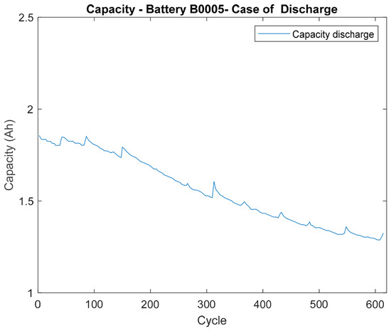
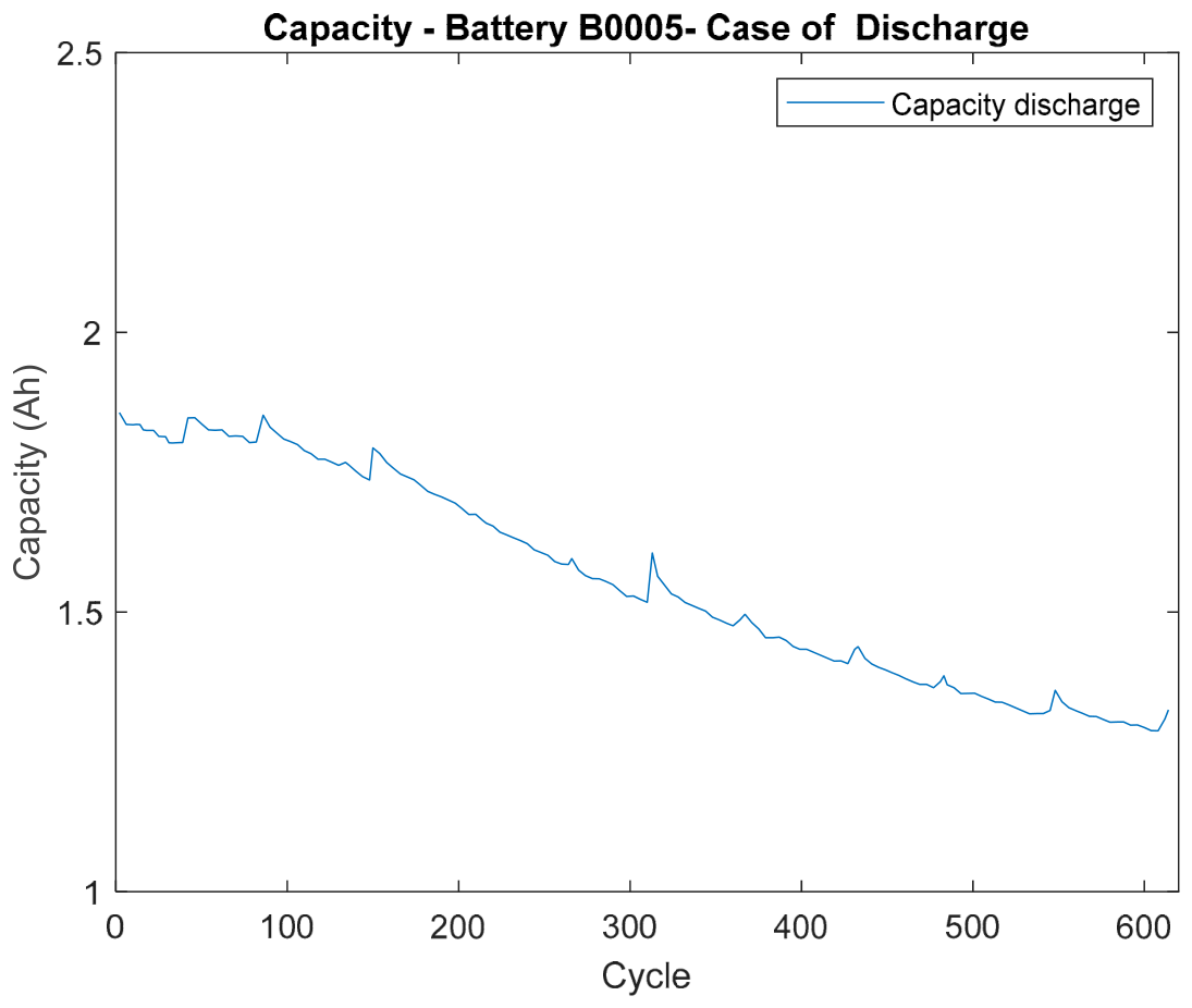
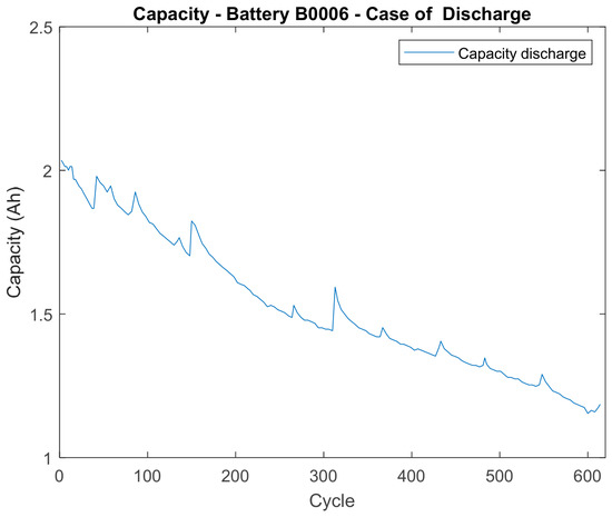
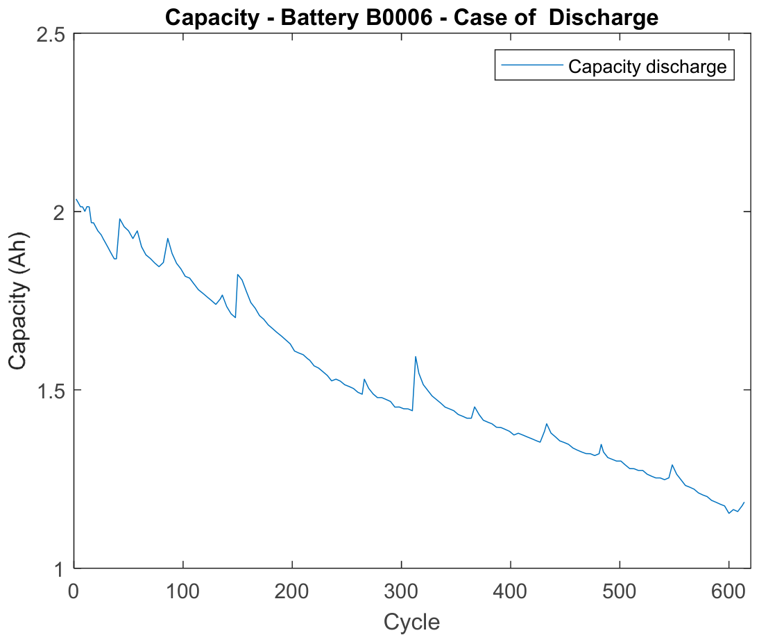
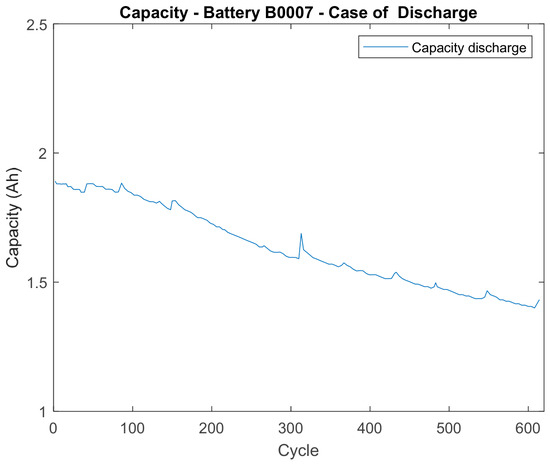
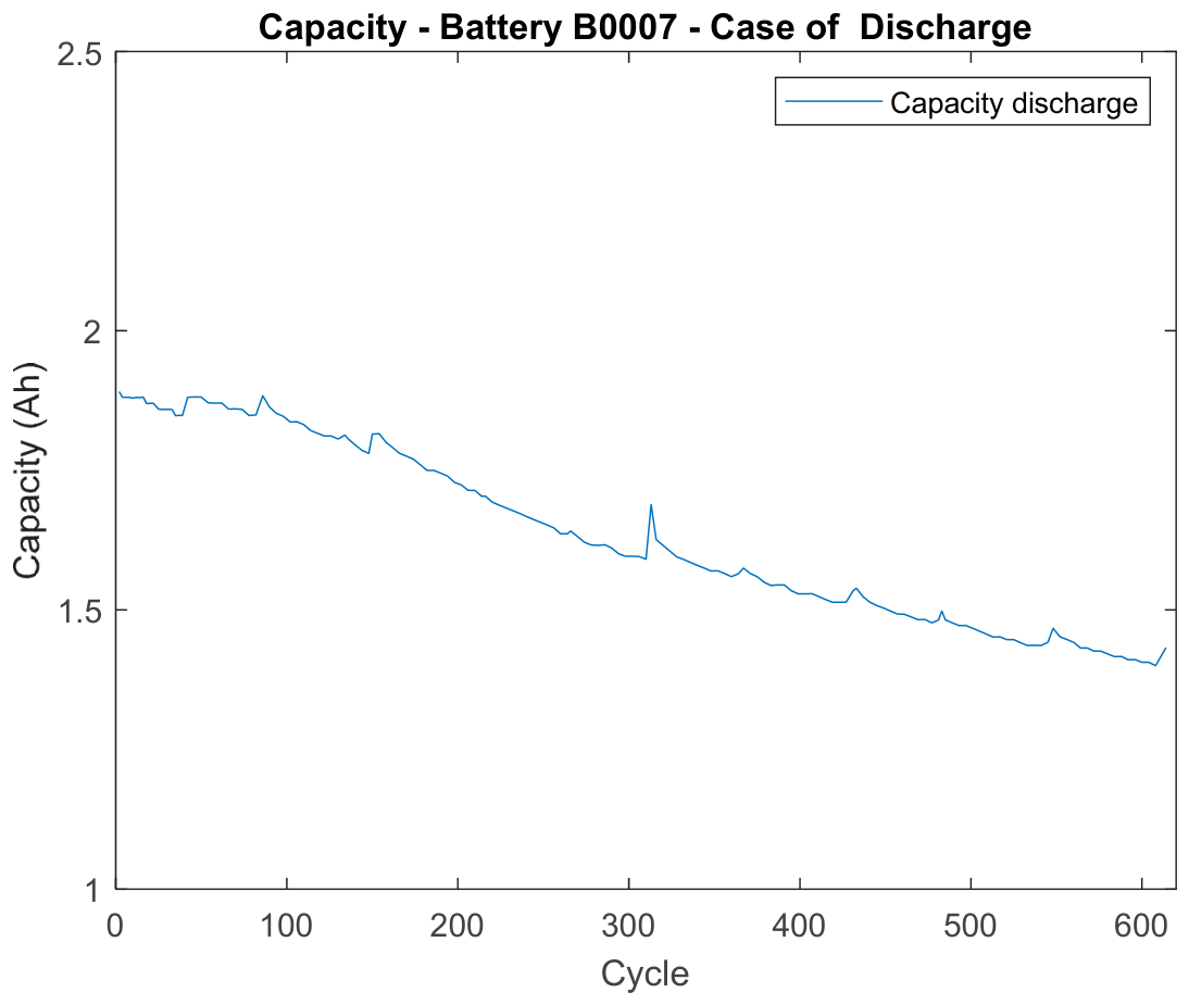
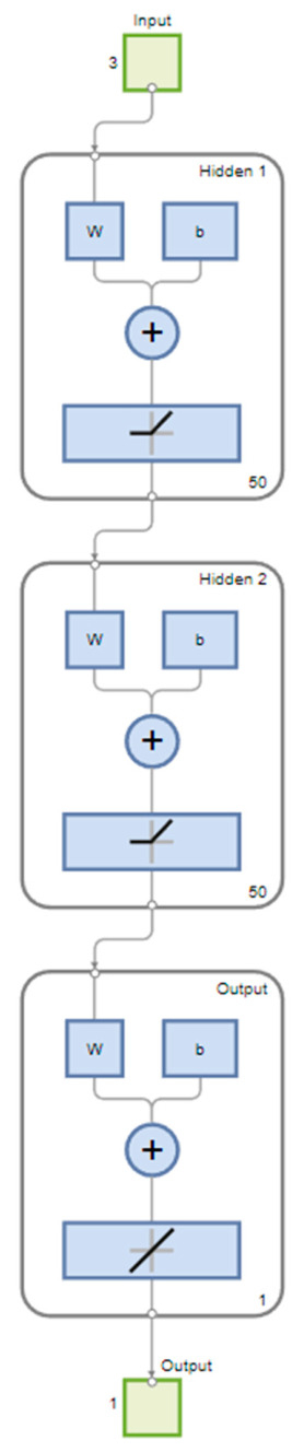
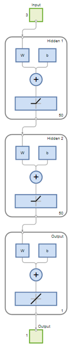
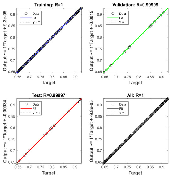
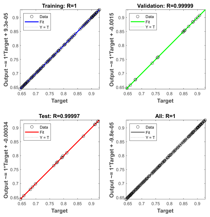
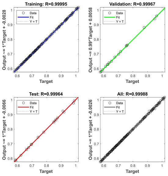
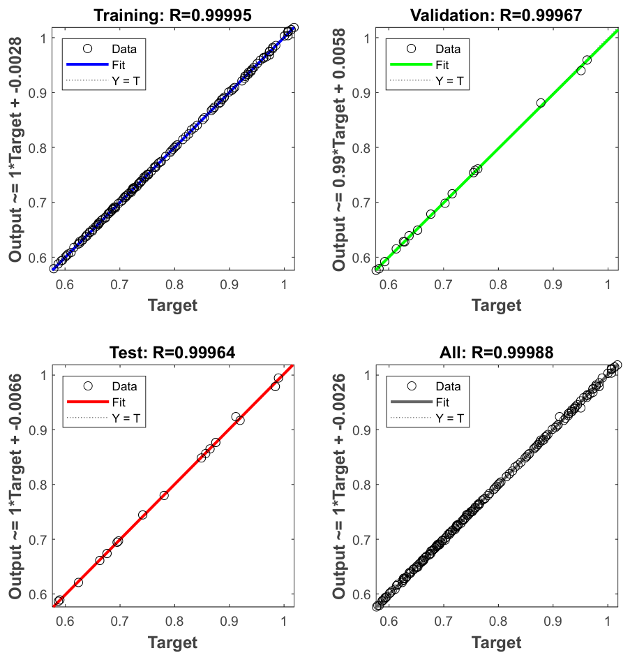
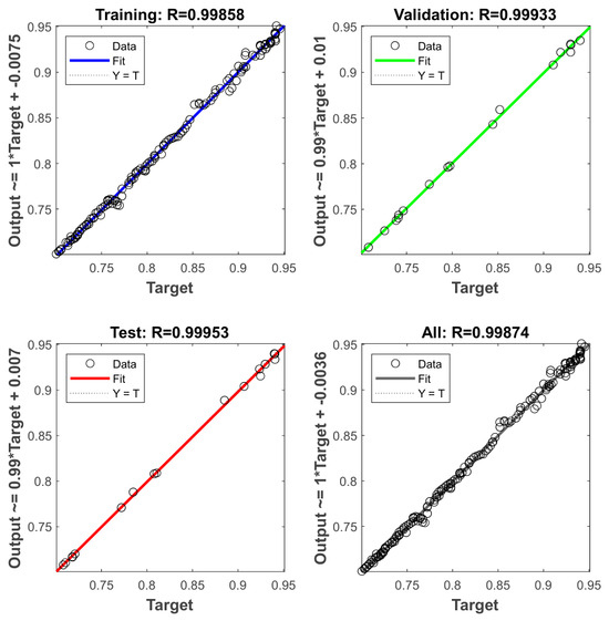
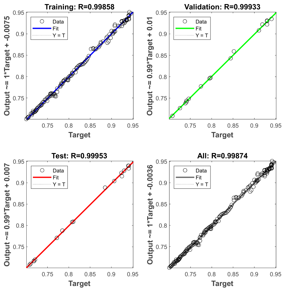
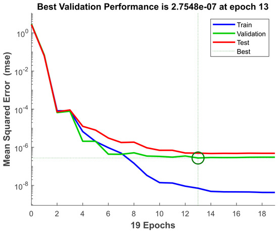
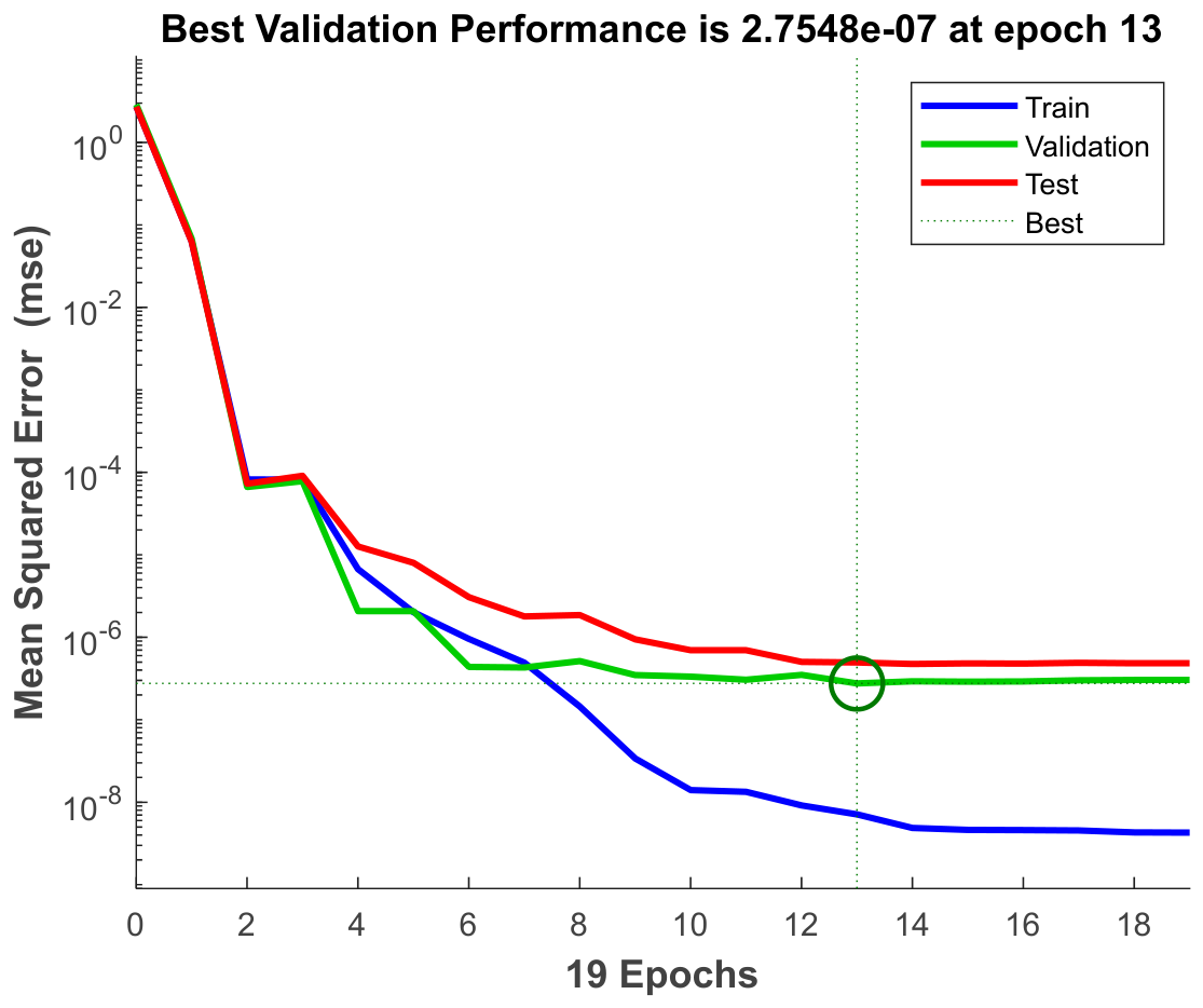
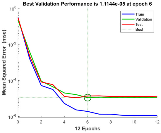
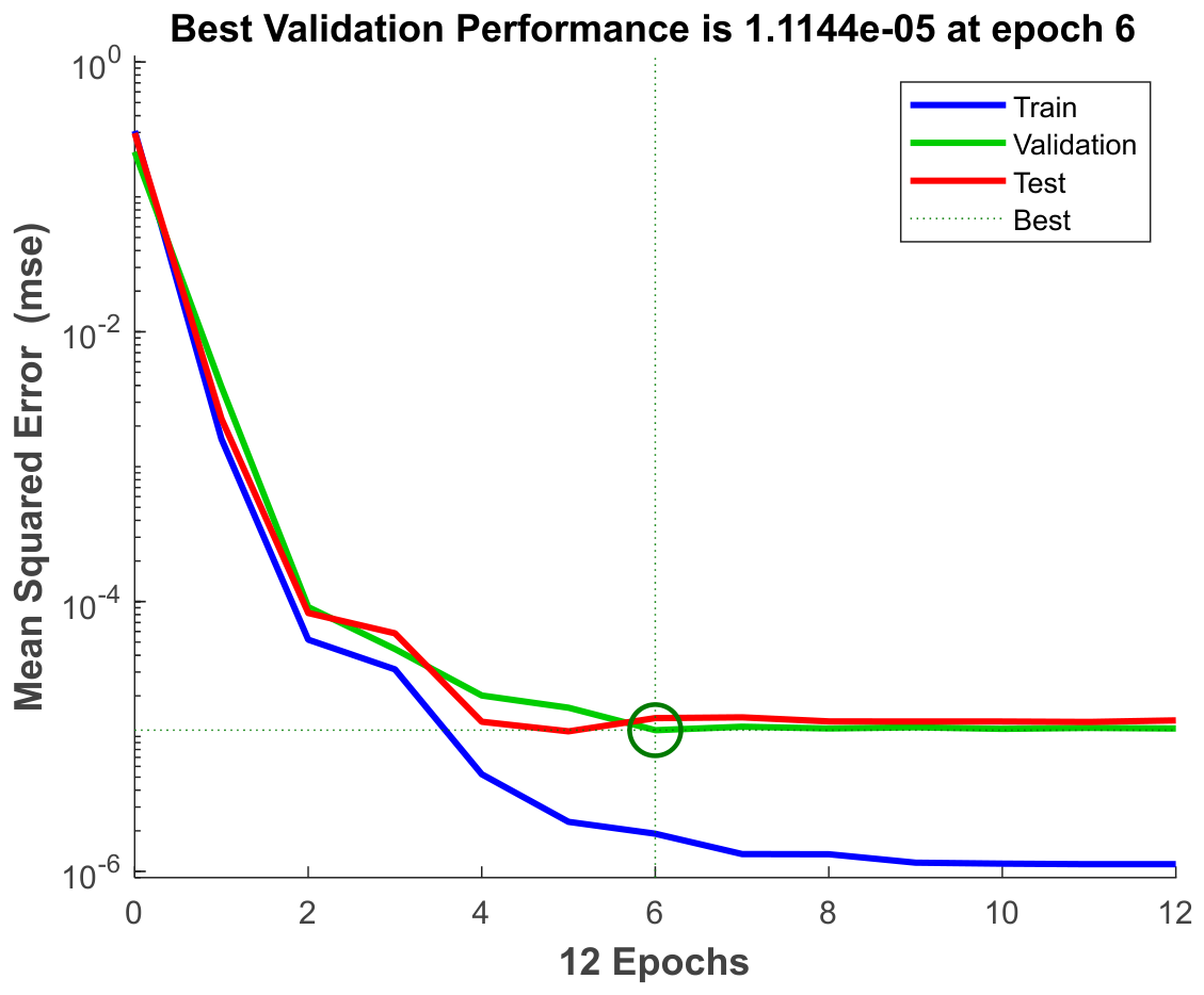
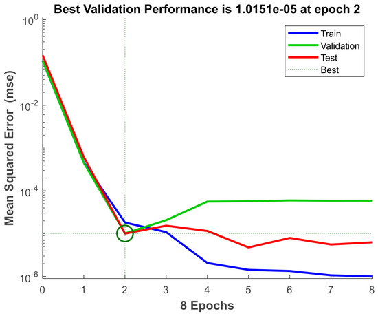
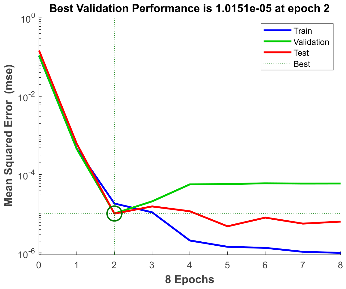
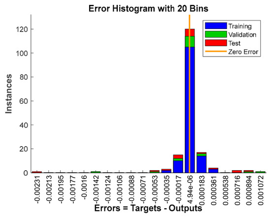
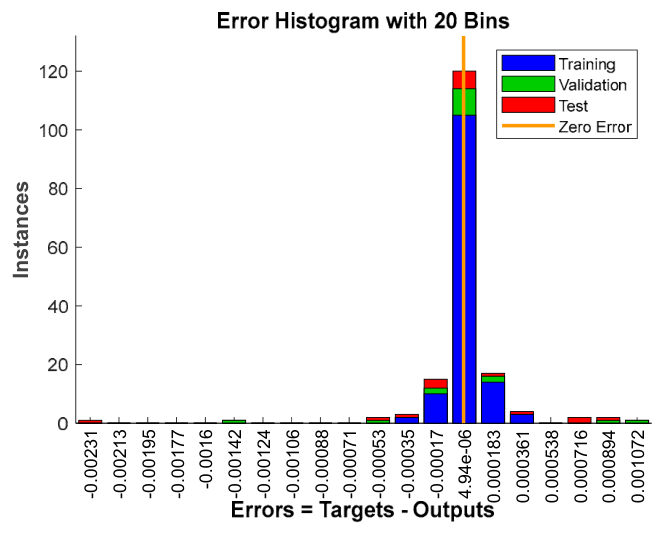
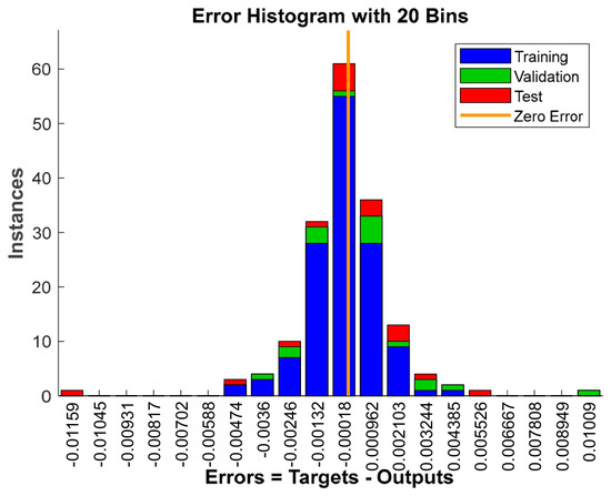
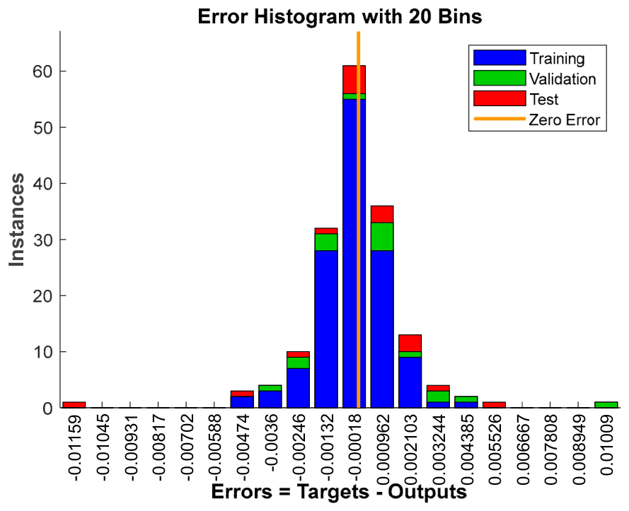
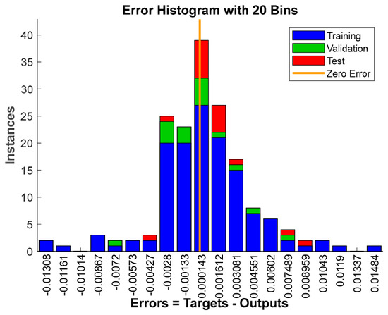
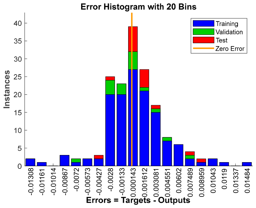
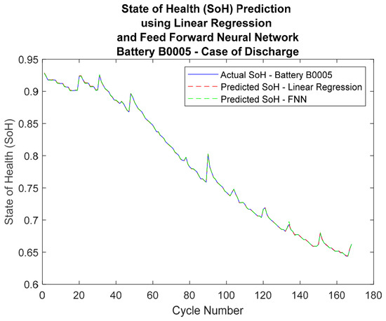
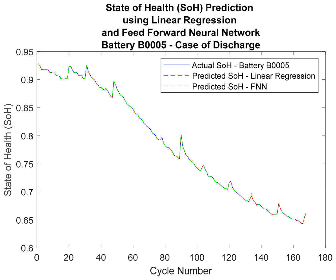
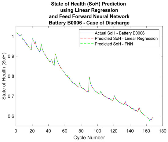
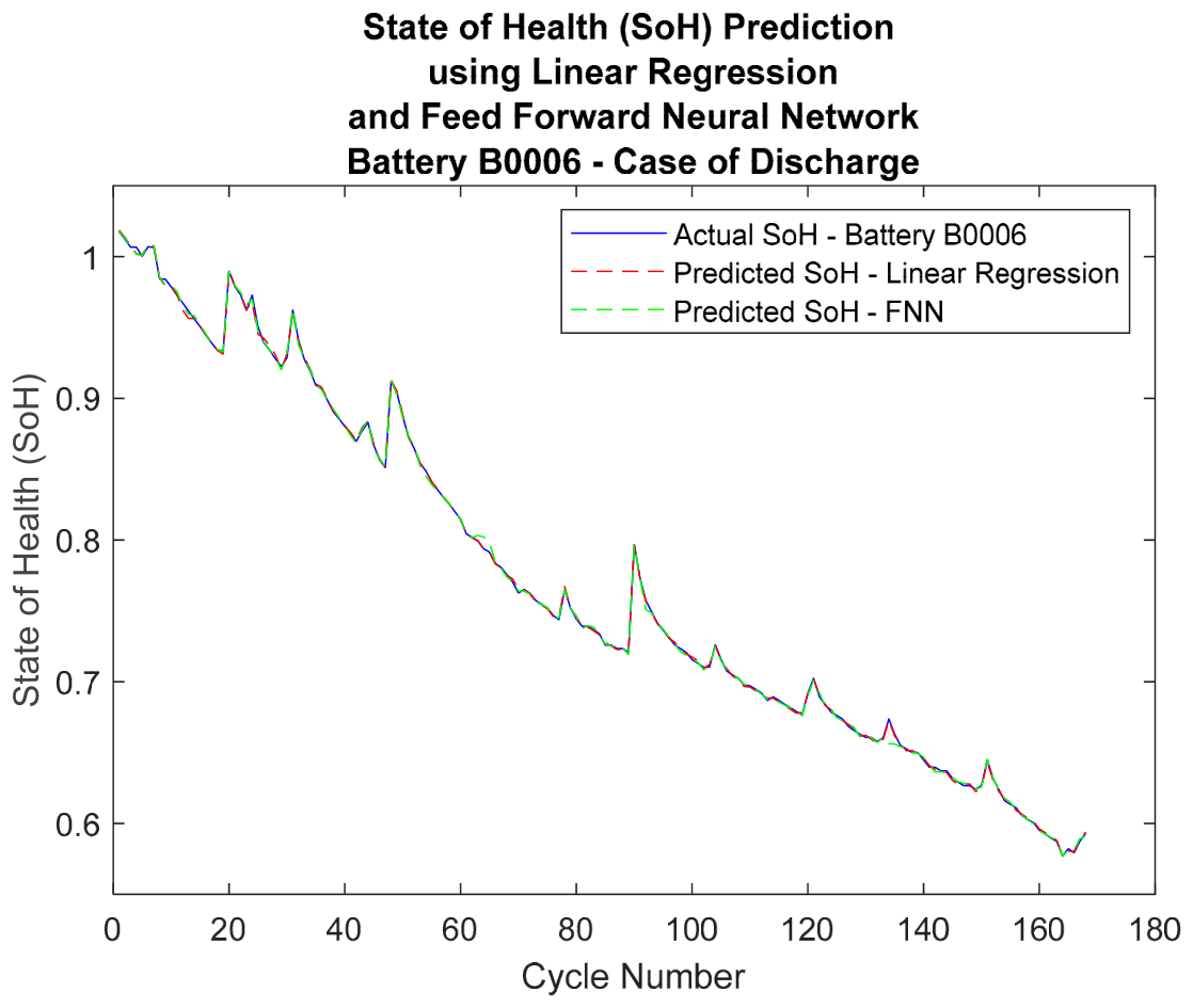
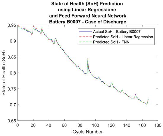
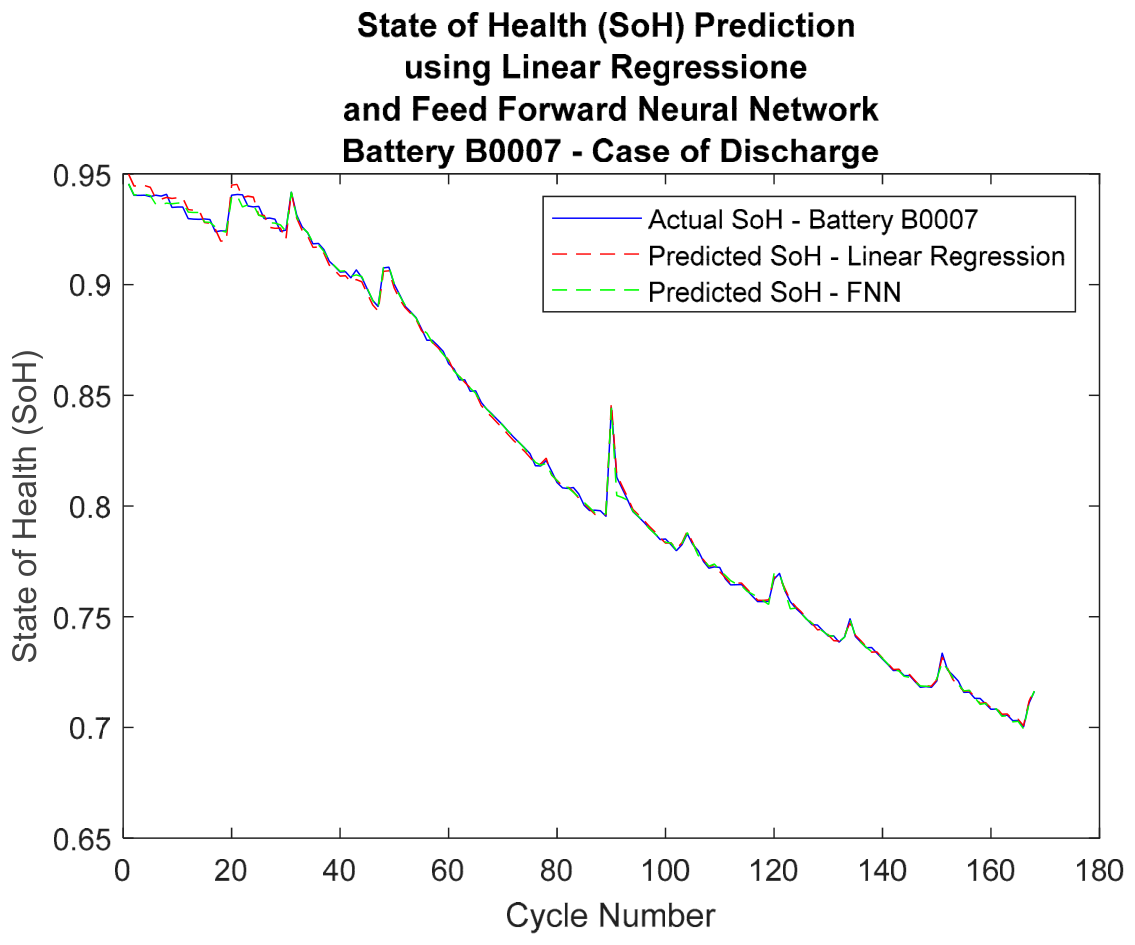

Disclaimer/Publisher’s Note: The statements, opinions and data contained in all publications are solely those of the individual author(s) and contributor(s) and not of MDPI and/or the editor(s). MDPI and/or the editor(s) disclaim responsibility for any injury to people or property resulting from any ideas, methods, instructions or products referred to in the content. |
© 2026 by the author. Published by MDPI on behalf of the World Electric Vehicle Association. Licensee MDPI, Basel, Switzerland. This article is an open access article distributed under the terms and conditions of the Creative Commons Attribution (CC BY) license.