


Abstract
Thermal management is a key factor for the efficiency, performance, and reliability of battery electric vehicles (BEVs), particularly in systems with strongly coupled components and heterogeneous thermal dynamics. This study proposes a centralized nonlinear model predictive control (NMPC) strategy for component cooling in BEVs, designed to maintain temperatures within optimal ranges while minimizing energy consumption and respecting actuator constraints. A reduced-order physics-based model is developed in MATLAB/Simulink R2024b, and the NMPC is implemented using CasADi, incorporating coolant temperatures as stabilizing states and a systematic parametrization of sampling time, prediction horizon, and weighting factors. The considered thermal management system consists of hydraulically coupled subsystems with different overall time constants, for which a single-horizon NMPC formulation is applied. Simulation results show that the proposed controller accurately tracks thermal dynamics across components with varying inertia and effectively captures cross-coupling effects. Sensitivity analyses indicate that variations in sampling time and prediction horizon have a limited impact on temperature trajectories and energy consumption, demonstrating robustness and real-time applicability. Compared to a rule-based controller, the NMPC achieves up to 30% reduction in energy consumption depending on ambient conditions and driving cycles, while improving temperature regulation, particularly for the high-voltage battery, with up to 2 K lower peak temperatures and a more balanced temperature distribution. These findings demonstrate that centralized NMPC is a suitable and efficient approach for thermal management in directly coupled BEV subsystems with heterogeneous dynamics.
1. Introduction
Effective thermal management is essential for ensuring the safety, efficiency, and longevity of battery electric vehicles (BEVs) and their components. The thermal management system (TMS) maintains optimal operating conditions for the high-voltage battery (HVB), electric motor (EM), power electronics, and other high-voltage (HV) components under varying environmental and load conditions. Since dynamic driving conditions significantly influence thermal loads and energy consumption, predictive control strategies have gained increasing attention as a means to improve overall system efficiency as investigated in [1,2]. In [3,4], it was shown that using optimization-based temperature regulation of the battery can improve the energy efficiency of the TMS compared to conventional approaches.
Cooling operation represents the dominant challenge in BEV thermal management. Limited heat exchanger capacity, strong dependence on ambient conditions, and large transient heat loads during high-power operation restrict the available cooling potential. In contrast, heating can be achieved more predictably using electrical heaters or heat pumps, although heat pump efficiency decreases at low ambient temperatures [5]. Consequently, advanced cooling control strategies are particularly relevant for improving system efficiency and component protection.
Conventional TMS control strategies are typically heuristic or rule-based (RB), relying on predefined temperature thresholds and sequential actuator logic. While robust and straightforward to implement, these approaches are inherently reactive and do not anticipate future thermal loads or subsystem interactions. As a result, actuator coordination is often suboptimal under dynamic driving conditions, leading to unnecessary energy consumption or uneven temperature distributions.
The increasing architectural complexity of modern BEVs introduces additional control challenges for the TMS. In many vehicle platforms, the coolant circuits of the HVB and EM are hydraulically and thermally coupled [6,7]. Shared coolant paths, controllable valves, and variable-speed pumps create strong cross-coupling effects between subsystems. Additionally, multiple interconnections between coolant loops at different temperature levels increase the available degrees of freedom in the system. Since HVB and EM components operate optimally in different temperature ranges, coordinated mixing of coolant flows can improve overall thermal efficiency. However, this coupling significantly enlarges the control space and complicates actuator coordination.
From a dynamical perspective, the coupled subsystems exhibit different overall thermal time scales. Due to its high thermal mass, the HVB evolves on comparatively slow time scales, whereas coolant temperatures and actuator dynamics respond faster. Multi-layer or multi-rate MPC formulations have been proposed for systems with pronounced time-scale separation [8,9]. However, in the considered TMS architecture, the dominant thermal states of the HVB and EM operate within comparable inertia ranges, and the faster fluid dynamics primarily act as internal coupling variables rather than independent control objectives. Therefore, the degree of time-scale separation is not sufficiently pronounced to warrant a hierarchical or multi-horizon optimization framework.
Furthermore, the strong hydraulic coupling between subsystems limits the applicability of hierarchical or multi-stage MPC approaches, in which subsystems are optimized sequentially or partially decoupled [10]. Valve positions and coolant mass flow rates simultaneously influence both thermal branches. Sequential optimization may therefore result in conflicting control actions or locally optimal yet globally suboptimal operating points. A centralized formulation is better suited to capture the interdependence between component temperatures, coolant states, actuator dynamics, and valve positions within a single optimization problem.
Although MPC-based automotive TMS control has been investigated in several studies [11,12,13,14,15], most contributions focus primarily on battery cooling circuits or on only thermally coupled subsystems. Strongly coupled multi-component cooling systems with shared hydraulic structures have received less attention. In such systems, accurate state-space modelling is crucial to represent thermal interactions and actuator coupling within the prediction model.
Considering these challenges, this work investigates a centralized nonlinear model predictive control (NMPC) approach for coupled BEV cooling systems. The controller is implemented within a high-fidelity, experimentally validated digital twin derived from first-principles physical equations. To ensure real-time feasibility, a reduced-order modelling approach is adopted that preserves dominant thermal dynamics while limiting computational complexity.
Although the coupled subsystems exhibit different overall thermal time constants, the dominant thermal states operate within comparable inertia ranges, and the hydraulic coupling introduces strong cross-dependencies between control inputs and subsystem temperatures. It is shown that, under these conditions, a centralized single-horizon NMPC formulation is sufficient to capture the relevant dynamics. This eliminates the need for multi-rate or hierarchical MPC architectures and avoids additional structural and computational complexity without sacrificing control performance.
A structured methodology for selecting sampling time, prediction horizon, control horizon, and cost-function weighting factors is proposed. The approach replaces heuristic tuning with a transparent and reproducible parametrization process, thereby reducing calibration effort and facilitating controller transferability to similar TMS configurations. A dedicated sensitivity study investigates the influence of the sampling time and prediction horizon on temperature regulation of components with different thermal inertia, and energy consumption.
The NMPC is formulated using a multi-objective cost function that simultaneously (i) maintains HVB and EM temperatures within optimal operating ranges, (ii) minimizes actuator energy consumption, and (iii) ensures smooth control actions to enhance actuator longevity. The proposed strategy is systematically compared to a conventional RB controller under various ambient temperatures and standardized driving cycles, evaluating thermal stability, energy efficiency, actuator coordination, and numerical robustness.
This publication is organized as follows. Section 2 presents the problem statement for applying NMPC to TMS and introduces the cooling architecture, designed for this study. Section 3 presents the physical modelling approach for the vehicle and its TMS, focusing on the physical equations that govern the coolant loop and heat exchange processes. Additionally, it details the mathematical formulations used to represent the TMS for prediction within the NMPC framework. Section 4 outlines the development of the nonlinear model predictive controller, including the formulation of the optimization problem, the structure of the cost function, and the constraints applied in the control problem. In Section 5 a parametric study is conducted to investigate the effects of sampling time, prediction horizon, control horizon and weighting factors on the objectives and stability of the controller. Section 6 presents simulation results comparing the NMPC strategy with a conventional RB controller across different standardized driving cycles and environmental conditions. A study on the coupling of subsystems with different thermal inertia, regarding the matching of the control objectives, is also conducted. Finally, Section 7 concludes the paper by summarizing the main findings and outlining potential directions for future research.
2. Problem Statement
The TMS used to implement and evaluate the proposed NMPC controller is illustrated in Figure 1. It comprises two separate coolant loops, one regulating the EM temperature and the other controlling the HVB. While the circuits can operate independently, they are hydraulically coupled via a central control valve that enables flow interaction between both branches. The HVB loop is additionally thermally connected to the refrigerant circuit of the air-conditioning (AC) system through a chiller.
Figure 1.
TMS separate cooling mode (a) and combined cooling mode (b).
The control objective is to maintain the HVB and EM within their respective optimal temperature ranges by coordinating the coolant, bypass, and expansion valves, and by regulating the coolant and air mass flow rates through the radiator and chiller. This study focuses exclusively on cooling operations under varying driving and ambient conditions. Charging and heating scenarios are not considered; therefore, components related to charging, such as the onboard charger, are modeled as constant thermal masses and do not actively participate in the TMS.
Due to the different optimal operating temperatures of the HVB and EM, two separate circuits are employed. The EM rejects heat to ambient air via a radiator equipped with an electric fan. Potential airflow restrictions, such as active grille shutters, are neglected. The HVB rejects heat indirectly through a coolant-to-refrigerant heat exchanger (chiller). Since the focus of this work is on coolant-circuit coordination, refrigerant-side dynamics are not modeled explicitly, and inlet refrigerant conditions at the chiller are assumed constant.
The TMS operates in two cooling modes. In the separate mode (Figure 1a), the HVB and EM are cooled independently via the chiller and radiator, respectively. This mode maximizes cooling performance for the HVB, making it suitable for high ambient temperatures and high-performance driving. However, it entails significant energy consumption, as chiller activation can reduce driving range by up to 10% depending on conditions [16]. In the combined mode (Figure 1b), both circuits are regulated via ambient air through the radiator while the chiller is bypassed. This mode is suitable for moderate or low ambient temperatures and low-performance driving, where the cooling demand is lower, resulting in significantly reduced TMS energy consumption. Under hot conditions or high-performance driving, short-term EM cooling via the chiller may be applied. In these cases, the strategy must account for thermal energy transferred from the EM to the HVB to avoid battery overheating and maintain a stable temperature profile.
The main control valve constitutes the central coupling element between the two circuits. By regulating the degree of hydraulic interconnection, it determines how coolant mass flow is distributed between the HVB and EM branches. This valve therefore directly links subsystems with different dominant thermal inertias: the HVB, characterized by high thermal mass and slow temperature evolution, and the EM cooling loop, which exhibits faster thermal responses due to lower thermal capacity. Adjustments of the main control valve simultaneously influence both subsystem temperatures. Increasing flow coupling may improve radiator utilization efficiency but can also transfer thermal disturbances between branches. Consequently, the valve introduces strong cross-coupling dynamics and prevents independent regulation of the subsystems. From a control perspective, it represents the primary source of interaction between slow battery dynamics and comparatively faster EM cooling dynamics.
Heat transfer in each branch is regulated by dedicated coolant pumps and bypass valves. The main control valve enables continuous transition between combined and separated operation. All valves operate with continuous control signals, where 0% corresponds to separated or bypass configuration and 100% to fully combined or cooling configuration. Proportional mixing allows partial interconnection of loops, preventing abrupt temperature gradients that could destabilize the controller or cause local undercooling. The coolant pumps and radiator fan are also continuously actuated within a normalized range of 0–100%. To prevent excessive actuator wear and oscillatory behaviour, constraints on minimum and maximum control increments are imposed. The high number of actuators, continuous control variables, and multiple operating modes significantly increase the dimension of the control problem. In particular, the presence of the hydraulically coupling main control valve transforms the system into a strongly interconnected multi-input multi-output (MIMO) structure. An optimal control formulation must therefore coordinate all actuators simultaneously while accounting for cross-coupling effects, differing thermal inertias, and energy-efficiency trade-offs to ensure stable, efficient, and reliable cooling performance.
3. Modeling Approach
Accurate system modelling is essential for MPC design, as the prediction model directly affects controller performance, numerical stability, predictive capability and constraint handling capability. This section presents the modelling approaches used to capture the dynamics and thermal behaviour of the digital twin of the TMS and to define the system’s state equations for MPC prediction. To ensure reliable state estimation and predictive performance, the MPC state equations are derived from a system model that has been experimentally validated under various driving scenarios and ambient conditions. The validation confirmed high modelling fidelity and accurate representation of system dynamics, making the developed model suitable as the basis for MPC design and implementation.
As illustrated in Figure 2, the model consists of three subsystems: the vehicle model, the thermohydraulic model, and the controller. The vehicle model computes heat generation in the components based on driving speed, vehicle properties, ambient temperature and road inclination. The heat flows, calculated in the vehicle model, are passed to the thermal model, where coolant and component temperatures are computed and defined as the states for the controller. The control inputs and system states will be discussed detailed in the subsequent sections.
Figure 2.
Model structure and interactions between the subsystems.
The thermohydraulic model captures heat transfer processes, coolant transport dynamics, and actuator effects. It computes the temperatures of the HVB, EM, and coolant circuits, which constitute the dominant thermal states of the system and are directly used in the NMPC prediction model. From a dynamical perspective, the model captures subsystems with different effective thermal inertias. The HVB is represented as a high thermal mass with slow temperature evolution, whereas the EM and coolant volumes exhibit comparatively faster dynamics due to lower heat capacity. Importantly, these states are not independent: the hydraulic interconnection via the main control valve introduces coupling terms in the energy balance equations, linking coolant temperatures and mass flow rates between both circuits. Consequently, temperature evolution in one branch influences the other through shared flow paths and mixing effects. Rather than separating slow and fast states into distinct prediction layers, the modelling approach preserves all dominant thermal dynamics within a unified state-space representation. Faster fluid dynamics are modeled in reduced-order form and primarily act as coupling and transport states, while slower component temperatures determine the long-term thermal behaviour. This structure enables the NMPC to account for cross-coupling effects without requiring multi-rate or hierarchical prediction schemes.
To maintain computational feasibility for real-time implementation, a reduced-order modelling approach is employed. Spatially distributed thermal phenomena are lumped into equivalent thermal masses, and coolant dynamics are represented using averaged temperatures and mass flow balances. This approach preserves dominant time constants and interaction mechanisms while limiting model order and nonlinear complexity. The resulting state vector consists primarily of component temperatures and coolant temperatures at key nodes within the circuits. Control inputs include pump speeds, radiator fan speed, and valve positions, including the main control valve that governs hydraulic coupling. The nonlinear state equations are derived from first-principles energy and mass balance relations and are discretized for use in the NMPC framework.
The model outputs include component temperatures, actuator power consumption, and heat rejection rates. These quantities provide quantitative performance metrics for evaluating thermal stability, energy efficiency, and actuator utilization under different operating conditions.
3.1. Vehicle Model
The vehicle submodel determines the traction power demand and the associated heat generation of the HVB and EM. These quantities serve as external disturbances for the thermohydraulic model and are calculated based on their respective efficiencies and the vehicle’s driving resistances [17]. The vehicle-related parameters required for the vehicle submodel are based on a representative Tesla Model 3 configuration reported in [18,19].
The total longitudinal driving resistance is obtained as the sum of aerodynamic drag, rolling resistance, acceleration resistance and slope resistance:
The required traction power is then obtained from the total resistance and vehicle velocity :
Considering the drivetrain efficiency , EM efficiency , energy conversion efficiency of HVB , regenerative braking efficiency and auxiliary power consumption , the battery load can be calculated as:
Using and the battery configuration, the power of an individual battery cell can be determined and scaled to the entire battery pack. All parameters required for this computation are either directly measurable or provided by manufacturer specifications.
Finally, the resulting electrical power flows are converted into heat generation terms for the EM and HVB based on their respective efficiencies. These heat losses constitute the primary thermal inputs to the thermohydraulic model and directly influence component temperature evolution within the MPC prediction framework.
3.2. Powertrain Thermal Submodel
The heat transfer from the EM to the coolant, is modeled as forced convection within internal round cooling channels. Since detailed information regarding the internal geometry of the EM cooling channels and the thermophysical properties of the associated thermal masses is not publicly available, the unknown channel parameters were calibrated to reproduce the measured coolant outlet temperature of the EM. After calibration, the model relies exclusively on physically motivated relationships. This is essential for NMPC, as it preserves predictive capability without resorting to purely black-box modelling approaches.
The thermal losses of the EM, representing the heat generated within the component, are computed using from Equation (2) together with the drivetrain efficiency .
The dynamic evolution of the EM temperature and the coolant temperature downstream of the EM is determined using a modified energy balance equation [20].
The convective heat transfer to the coolant is given by:
with the overall heat transfer coefficient
where , , , and denote the Nusselt number of the coolant flow in the cooling channels, the thermal conductivity of the coolant, the hydraulic diameter of the cooling channels, the heat transfer area of the EM and the overall EM heat transfer coefficient, respectively.
The modeling of the convective heat transfer is based on established Nusselt correlations reported in [20], which are implemented in a flow regime-dependent formulation. In contrast to quasi-static approaches, the heat transfer coefficient is evaluated dynamically using instantaneous flow conditions and temperature-dependent thermophysical fluid properties.
The Reynolds number is computed from the coolant mass flow rate and temperature-dependent fluid properties, while the Prandtl number and thermal conductivity are updated as functions of temperature. Based on these quantities, the Nusselt number is determined according to the local flow regime.
To account for non-linear fluid behaviour, the model distinguishes between laminar, transitional and turbulent flow regimes using lower and upper Reynolds number thresholds and . For laminar flow , a constant Nusselt number of = 3.66 is assumed, corresponding to fully developed laminar flow in a circular pipe with constant wall temperature as described in [20].
For turbulent flow , the Gnielinski correlation [20] is used to estimate the Nusselt number in the moderate and fully developed turbulent regime. This correlation provides improved predictive accuracy compared to simpler empirical relations, as it explicitly incorporates the Darcy friction factor and thereby accounts for wall effects and flow resistance.
In the transitional regime , the Nusselt number is formulated using a normalized Reynolds number, consistent with standard approaches for regime blending in convective heat transfer correlations [21]. Rather than applying a linear interpolation between the laminar and turbulent Nusselt numbers, a cubic Hermite interpolation is employed to ensure a continuously differentiable transition between flow regimes. A normalized Reynolds number is defined as:
The weighting function is given by:
The resulting Nusselt number in the transitional regime is then computed as:
This formulation ensures a smooth and physically consistent transition of the heat transfer coefficient across flow regimes, eliminating discontinuities that could negatively affect numerical stability. Consequently, the model captures regime-dependent heat transfer behaviour while remaining suitable for real-time NMPC, even under rapidly varying operating conditions.
This regime-dependent formulation is well suited to thermal management applications with internal circular cooling channels, where the coolant flow commonly spans laminar, transitional and turbulent regimes depending on operating conditions. Overall, the approach ensures physical consistency and robust prediction accuracy of convective heat transfer coefficients across the entire operating range.
In [22], it was shown that a simplified thermal model of the electric machine with constant thermophysical properties yields negligible deviations compared to experimental measurements. For modelling simplicity and computational efficiency, the specific heat capacity of the EM’s thermal mass is assumed constant over the operating temperature range.
The effective coolant temperature inside the EM is obtained from the inlet and outlet coolant temperatures [23]. Substituting Equation (11) into the energy balance defined in Equation (6) yields the coolant outlet temperature:
Substituting this relation into the energy balance yields the coolant outlet temperature:
where denotes the coolant specific heat capacity and is the coolant mass flow rate through the EM.
Finally, the heat transported by the coolant through the EM, , is calculated as:
3.3. Battery Thermal Submodel
An electrical equivalent circuit model (ECM) with two elements is used to describe the electrothermal behaviour of the HVB [24]. In this study, cylindrical lithium-ion cells are considered, with cooling provided by parallel coolant channels positioned between the cells, as described in [19]. All cells are assumed to be identical, without variations in load or capacity, allowing the modelling of a single representative cell. Based on the battery load calculated in Equation (3), along with the battery configuration and cell electrical parameters, the current of an individual cell can be determined. Using the cell current, the heat loss of the battery pack can then be calculated. The total heat loss consists of an irreversible portion and a reversible portion :
The irreversible heat generation results from the cell’s internal resistance and cell current , while the reversible component is determined from the entropic coefficients , which depend on the open-circuit voltage at different temperatures [25].
Heat transfer from the HVB to the coolant is modeled using a convective approach [20]:
with the overall heat transfer coefficient and the effective coolant temperature
where , , and representing the Nusselt number of the coolant flow, the coolant thermal conductivity, the hydraulic diameter of the cooling channels and the overall HVB heat transfer coefficient, respectively.
The thermal dynamics of the HVB are described using an energy balance [23]:
where is the battery temperature, is the battery mass, is the heat capacity and is the heat transfer rate from the HVB to the coolant. The heat transfer coefficient of the HVB is calculated analogously to that of the EM component, as described in Section 3.2. Under realistic operating conditions, including cooling operations and cooldown from the soaked temperature, the HVB temperature varies only within a range of approximately 25 K. Consequently, the resulting temperature dependence of the specific heat capacity is considered negligible over the investigated operating range. Therefore, the heat capacity of the HVB, is assumed to be constant over the considered operating conditions. The effective coolant temperature is calculated similarly to Equation (11), using HVB inlet and outlet coolant temperatures.
The coolant outlet temperature can then be expressed analogously to that of the EM using the heat transfer rate to the coolant, defined in Equation (17):
where is the coolant mass flow rate through the HVB.
Finally, the heat transported by the coolant mass flow is defined as:
3.4. Model of the Thermal Management System
Within the TMS, the pipe sections between components are modeled under the assumption of being adiabatic to the ambient. This simplification is justified by their close integration with surrounding vehicle components, which exchange heat among each other and with the environment.
As illustrated in Figure 1, the coolant flow can be split into the EM and HVB cooling loops by a three-way control valve, resulting in mass flow rates and , respectively. In the EM cooling loop, the coolant can bypass the cooler via a bypass path, while in the AC system, cooling through the chiller can be deactivated by redirecting the refrigerant flow through an electrically controlled expansion valve. In combined cooling mode, the EM circuit pump controls the mass flow, with the HVB pump synchronized accordingly. In separate mode, each pump is controlled independently based on the cooling requirements of the respective components.
The coolant mass flow rates within the system are determined using the principle of mass conservation, defined as functions of the pump-generated flow and control valve positions:
Using Equations (13)–(22), the cooling power in each circuit is calculated from the heat transfer within the respective heat exchangers:
Here, is the minimum heat capacity rate between the two fluids in the heat exchanger, respectively, as defined in the effectiveness-Number of Transfer Units (-NTU) method [26].
The thermophysical properties of the coolant, refrigerant, and air are obtained from the open-source database CoolProp [27]. The refrigerant mass flow rate through the chiller is assumed to be constant, as the air-conditioning system dynamics are not explicitly modeled in this study and are outside the scope of the present work. The chiller is represented by an ideal vapor-compression cycle in which the refrigerant is assumed to be fully evaporated, enabling a reduced-complexity model focused on coolant circuit dynamics. Phase change effects in the refrigerant cycle are therefore not explicitly modeled, as no phase change occurs within the considered operating range of the system.
Under this assumption, constant thermophysical properties can be applied for a given refrigerant mass flow rate. The assumed constant refrigerant mass flow rate represents typical operating conditions of automotive air conditioning systems for the studied vehicle performance class. Under these assumptions, the temperatures throughout the TMS can be computed consistently.
In addition to thermal efficiency, energy efficiency is also included among the control objectives. Electrical power consumption is described as a function of pump and fan rotational speeds, valve control frequencies, and their respective maximum power. Pumps exhibit an approximately cubic relationship between rotational speed and mechanical power, while fans follow a quadratic relationship. Mixing valves are neglected due to their comparatively low power consumption. The overall TMS electrical energy consumption is given by
The electrical power of each actuator is calculated from its mechanical power and efficiency:
where and represent the mechanical power, are dependent on the pump rotational speed, and are obtained from the component characteristic maps provided by the manufacturer.
4. Control Problem Formulation
The following section presents the formulation of the NMPC controller, including the formulation of the cost function and the state equations for the prediction model. The objective is to optimally coordinate distributed thermal actuators under dynamic driving conditions while explicitly accounting for thermal coupling, actuator limitations, and energy efficiency.
Using the equations of the designed model, MPC is capable to predict the system’s future behaviour by formulating the dynamics as ordinary differential equations (ODEs). The system dynamics are represented in continuous-time nonlinear state-space form
where denotes the system’s states, the control inputs, and the time-invariant system parameters. The state variables are selected to ensure they are measurable in a real-world vehicle. The prediction model includes six state variables
and five control inputs
and four disturbances
The inclusion of coolant temperatures as states is essential. They capture the thermal coupling between subsystems, transport delays within coolant circuits and storage effects due to distributed thermal masses. Neglecting these intermediate thermal states would result in an incomplete representation of internal heat accumulation and delayed heat rejection. First-order filters are applied to the controller to capture the thermal inertia of the state variables and improve the accuracy of the prediction model, as shown in Equation (31), where all variables are defined in the previous section.
The controller pursues three objectives: first, maintaining a uniform HVB temperature distribution and keeping the EM below its upper temperature limit while avoiding undercooling or overheating; second, ensuring smooth actuator operation to improve energy efficiency; and third, ensuring a more balanced coolant temperature for stable system operation and component temperature regulation. To achieve these objectives, a discrete-time finite-horizon optimal control problem (OCP) is formulated as:
The cost function represents the weighted sum of temperature tracking errors, actuator power consumption, and control move magnitudes. denotes the number of prediction steps and is the sampling time of the discrete prediction model. In the cost function, denotes the weighting factors, the change in rotational speed of the fan and pumps, and the change in the valve control signals. The temperature states and are defined in Equation (5) and Equation (20), respectively. It should be noted that the optimization problem becomes nonlinear primarily due to the formulation presented in Equation (15). Consequently, NMPC is implemented using the sequential quadratic programming method (SQP) [28,29,30]. A tracking term for the coolant temperature is also introduced to achieve a more stable thermal operation of the system, resulting in more uniform actuator control.
The cost function is composed of multiple terms: (1) three temperature tracking terms for the HVB and EM component temperatures, and for the coolant temperature at the outlet of the radiator, which drive the respective temperatures toward their reference values and optimal ranges; (2) two power consumption terms corresponding to the controlled actuators, representing the energy efficiency objectives of the controller; (3) one control move penalty term for the coolant pumps and fan, which limits rapid and large changes in actuator control inputs to promote smooth operation; (4) One control move penalty term for valve switching, to reduce frequent or abrupt valve operations.
Energy consumption is directly incorporated using physically derived actuator power models. Unlike heuristic penalties on control signals, this term reflects actual electrical consumption, enabling thermally optimal yet energy-aware operation. Constraints on the minimum and maximum changes in the control signals, the lower and upper bounds for the actuators, and the allowable ranges of the states are applied to ensure safe and feasible system operation. These constraints prevent excessive or abrupt actuator movements, protect components from operating outside their physical limits, and maintain the prediction model within realistic bounds, thereby enhancing control stability and reliability.
The coolant temperature at the radiator outlet is a direct measure of the EM-circuit’s heat dissipation capacity. The temperature dynamics of the coolant exhibit delays and storage effects determined by heat transport and transfer within the circuit. If the controller only considers the EM temperature, potential heat buildup in the cooling system may not be captured. This can lead to increased coolant temperatures, which may initially have little effect on the EM temperature but can compromise system efficiency and long-term safety. Maintaining a balanced coolant temperature also enables rapid response to sudden changes in load. The additional penalization integrates a thermal intermediate state that better reflects the effects of cooling performance fluctuations, enhancing the robustness of the control strategy. It also reduces thermal stress on the cooling system overall, helping to protect components and extend their lifespan. Since the coolant temperature at the radiator outlet directly impacts the EM temperature, it is weighted with the same factor . This approach also reduces the complexity of the cost function by limiting the number of terms, leading to faster convergence and more stable NMPC operation.
The power consumption of the pumps and fan is not explicitly penalized, as their operation is governed by thermal requirements to ensure adequate cooling. Including it in the cost function would have a minimal effect while increasing the complexity of the optimization.
To protect the actuators from frequent changes in operating states, minimum hold times were defined for each control signal, considering the dynamics of the respective actuators. For the valves, this minimum duration was set to 30 s, while for the fan and pumps it was set to 20 s. To prevent excessive controller response to short-term thermal spikes, first-order filters are applied to the calculated heat flow inputs.
In addition to the cost function, the NMPC formulation includes a set of constraints: soft constraints for component temperatures, operational limits on the control inputs, and bounds on the rate of change in these inputs. The desired operating temperature range for the HVB is set at 30 °C with a permitted deviation of +4 °C and −2 °C, as the optimal operating temperature range is defined between 15 °C and 40 °C as stated in [31,32]. For the EM, the maximum operating temperature is defined at 180 °C in [33]; therefore, the operating temperature range of the EM is defined between 120 °C and 180 °C with soft constraints and an optimum of 150 °C. Maintaining a constant high EM temperature is not optimal for component health, as prolonged exposure can accelerate aging. Allowing a defined temperature range with a maximum upper bound enables the EM to tolerate short periods of higher temperatures without compromising lifespan, while avoiding unnecessary cooling and improving overall system efficiency. In the controller, states and input variables are constrained with minimum and maximum threshold values to ensure a stable operation within desirable conditions.
Considering the ram air effect at the front of the vehicle, the fan operating bounds are defined as a function of vehicle speed. This approach allows the fan to remain inactive when its operation would not significantly increase airflow through the radiator at higher speeds. Due to rapid fluctuations in vehicle speed, which directly influence fan effectiveness, soft constraints are applied to the fan bounds. This ensures numerical stability and avoids infeasibility in the optimization problem caused by abrupt airflow changes. To model airflow inertia, a first-order transfer function was implemented. Similarly, first-order filters were applied to capture the thermal inertia of the components’ thermal masses. Additionally, the hydraulic inertia of the pumps and fan was modeled using first-order transfer functions, providing a realistic and stable representation of actuator behaviour within the control framework.
The simulations were conducted on a desktop computer with an AMD Ryzen 5 six-core 3.6GHz processor. The optimal control problem was formulated and solved using the Interior Point OPTimizer (IPOPT) [34] within the CasADi [35] framework in MATLAB R2024b. Various initial ambient conditions and driving scenarios were considered throughout the simulations; these are discussed in detail in Section 6.
5. NMPC Parametrization
To evaluate the efficiency and performance of the NMPC developed in the previous section, appropriate parameterization is essential. In particular, an optimal balance must be achieved between computational effort, control performance, optimization stability, and prediction accuracy. This balance depends critically on the selection of four key parameters: the controller’s sampling time, prediction horizon, control horizon and the weighting factors.
The parametric study was conducted in a closed-loop simulation using a driving cycle that combines the WLTP3 and Artemis Highway (150 km/h) profiles at an ambient temperature of 35 °C. This setup ensures that both urban and highway driving scenarios are represented within a single simulation under moderately elevated ambient conditions. To introduce realistic disturbances and test robustness, randomly generated road inclinations were applied, simulating variable vehicle loads and introducing unmeasurable, non-predictable effects into the control system.
Before initiating fine-tuning of the NMPC, an initial set of parameter values was identified to ensure stable controller operation and full actuation of all controlled components. This step guarantees that the controller can effectively interact with all actuators and that the controlled signals are coordinated, with system dependencies accurately represented.
The fine-tuning process proceeds in two main steps. First, the prediction horizon, control horizon, and sampling time of the controller are optimized to balance computational efficiency, control accuracy and stability. Second, the weighting factors in the NMPC cost function are determined by minimizing the squared error between the closed-loop response of the controller and the predefined reference trajectory. This approach ensures that the controller achieves both high performance in terms of temperature regulation and actuator coordination, while maintaining low computational cost for real-time applicability.
5.1. Sampling Time
The sampling time directly influences the computational load of the NMPC, as it determines how frequently the algorithm is executed during a given driving scenario. A shorter sampling time allows the controller to react more quickly to disturbances and can improve tracking accuracy; however, it also increases computational demand, potentially making real-time implementation infeasible. Conversely, a long sampling time may fail to capture the system’s current state with sufficient fidelity, resulting in slower responses to disturbances and degraded performance [36].
Since the investigated TMS exhibits relatively slow thermal dynamics in response to control actions and load variations, a parametric study was carried out for values ranging from 0.5 s to 10 s. The analysis focused on performance, robustness, and fulfilment of the cost function objectives. At this stage, prediction and control horizons as well as weighting factors were kept at initial, non-optimized values; thus, results serve primarily as relative performance indicators.
The upper diagram in Figure 3 presents the total accumulated cost for different values over the entire driving cycle. The cost reflects deviations from the temperature references, high electrical energy consumption, and rapid changes in the control signals, with higher costs indicating poorer overall performance. At very small , frequent optimization may induce overreactions and increase sensitivity to noise, although no significant instabilities were observed between consecutive steps. Since optimization outcomes are coupled with the horizon lengths, some cost variations are expected to change after horizon tuning.
Figure 3.
NMPC performance over different sampling times.
The middle diagram of Figure 3 shows that the solver consistently converged within the maximum allowed iterations for between 0.5 s and 2 s. For values up to 8 s, the rate of failed optimization steps remained acceptable. However, at 10 s, numerical convergence problems became significant, indicating a loss of control resolution and feasibility.
In real-world applications, real-time feasibility is crucial. Short sampling times reduce the available computation window, potentially causing premature solver termination and suboptimal solutions. Given the relatively slow system dynamics, using as small as 0.5 s offers negligible benefit and may be counterproductive.
The lower diagram in Figure 3 shows an almost linear increase in computation time per , except at 2 s, where a sharp rise occurs. This anomaly stems from the fixed prediction and control horizons, which in this configuration create a mismatch between the prediction window and effective control authority. The resulting ill-conditioned optimization problem increases nonlinearity and reduces degrees of freedom, leading to more iterations and longer solve times. This configuration induces a numerical issue, evident in the sharp rise in solver iteration count and simulation time. Overall, this behaviour highlights the sensitivity of MPC performance to the interaction between sampling time, horizon lengths, and the dynamics of the system. Since NMPC relies on a discrete-time model to predict future system behaviour, a larger increases the time step in the discretization of the underlying continuous-time nonlinear dynamics. This reduces model accuracy, making the optimizer’s predicted trajectories less reliable and increasing the likelihood of infeasible or unstable solutions, as illustrated in the middle diagram after 9s of sampling time.
The diagrams in Figure 4 illustrate how varying sampling time affects the control objectives. The results indicate that moderate sampling times, specifically between 2 and 5 s, provide the best overall balance across all objectives. Within this range, the controller effectively limits positive temperature deviations while maintaining low energy consumption of the TMS.
Figure 4.
Dependence of NMPC cost function objectives on the sampling time.
Although battery temperature control is generally less sensitive to changes in Ts, positive deviations are still minimized in this optimal range, as depicted in Figure 4 on the upper diagram. In contrast, sampling times greater than 5 s lead to increased temperature fluctuations and higher energy usage due to reduced control resolution and delayed actuation responses. Conversely, very small sampling times offer slightly better temperature control, but at the cost of increased computational demand and potential sensitivity to disturbances.
Considering both controller performance and control objectives, a sampling time of 5 s is selected for further parameterization, as it provides high stability, real-time computational feasibility, low overall cost, and a favourable trade-off between the objectives.
5.2. Prediction and Control Horizon
With the sampling time fixed at Ts = 5 s, the prediction and control horizons are optimized to further enhance NMPC performance. The slow thermal dynamics of the TMS suggest that a relatively long prediction horizon is advantageous for anticipating future states and disturbances [37]. In this study, a range of prediction steps, ph = [5, 15], and control steps, ch = [2, 5], was investigated, as values outside this range caused the control objectives to exceed acceptable limits. The range of ph was selected based on the chosen sampling time, corresponding to a prediction window of 25 to 75 s, providing a trade-off between accurate future state estimation, feasible computational effort, and rapid response to load and ambient changes. The control horizon was kept shorter than the prediction horizon to ensure the controller can effectively optimize future control actions; longer control horizons increase the number of decision variables, solver iterations, and computational complexity, potentially compromising numerical robustness and stability. An intermediate control horizon reduces solver load while maintaining predictive performance.
Figure 5 summarizes the impact of ph and ch combinations on four primary objectives, with respect to the NMPC stability over the whole driving cycle, average positive temperature deviation of the HVB and the coolant at the outlet of the radiator as well as the total energy consumption of the TMS. It should be noted that the average positive deviation of the HVB also includes the temperature deviation during the cooldown phase.
Figure 5.
Influence of number of prediction and control steps on the controller objectives and performance.
Based on the well-defined sampling time, the controller finds an optimal solution for the OCP in the range of ph = [8, 15] and control steps ch = [2, 4] for every combination. This is a critical requirement for real-time implementation, as solver divergence would render the controller unusable in practice. Solver failures encompass instances where the solver reaches the maximum number of iterations without satisfying the stopping criteria, resulting in non-convergence, as well as cases of complete failure due to numerical issues. Larger ch/ph ratios tend to increase the risk of solver instability by over-constraining the optimization problem with an excessive number of decision variables and reducing numerical robustness in the early prediction steps.
In NMPC, however, extending the control horizon increases the dimensionality of the optimization problem solved at each sampling instant. Specifically, a longer horizon introduces additional decision variables and constraints, as the control sequence must be optimized over more time steps. Furthermore, the system model must be propagated over the extended horizon during each iteration, increasing the number of nonlinear model evaluations. Since the computational complexity of nonlinear programming solvers generally scales superlinearly with the number of variables and constraints, the overall computation time grows accordingly.
Longer prediction horizons improve foresight over slow thermal dynamics, enabling precise regulation of HVB and coolant temperatures. For instance, ch = 3 combined with ph = 12 yields an HVB deviation of 2.16 K and a radiator outlet coolant deviation of 1.28 K, among the lowest across tested configurations. While longer control horizons can improve energy efficiency by enabling finer-grained control, they also increase computational complexity. The combination ch = 3 and ch = 12 achieves a total TMS energy consumption of 109 Wh over the driving cycle, demonstrating efficient thermal regulation without excessive actuator effort.
Temperature deviations will also vary significantly depending on the selected weighting factors in the cost function, as these determine the controller’s prioritization. The results indicate that an intermediate control effort, with ch = 3 and with a sufficient prediction depth of ph = 12, enables efficient operation without overheating or excessive actuation.
This configuration balances control granularity and predictive foresight: the moderate control horizon prevents over-constraining the optimizer and maintains solver stability, while the sufficiently long prediction horizon captures slow thermal dynamics for accurate temperature tracking. Consequently, energy consumption is minimized without compromising thermal performance, providing a practical and well-balanced NMPC design.
5.3. Weighting Factors
After ensuring the stability and performance of the controller using the optimal sampling time and horizon settings, the next step is to determine the optimal weighting factors based on the controller’s objectives. To determine the optimal weighting factors, they are grouped according to the control objectives. First, the weights and , related to component temperature regulation are varied. Second, the weighting factors and , primarily associated with power consumption and consequently affecting the temperature regulation, and secondarily influencing the cooling mode and mechanical protection of the actuators, are tuned. This structured approach enables a systematic evaluation of each objective’s impact on overall controller performance, while also considering the relative priority of the objectives.
The initial focus is placed on the thermal regulation of the components within the TMS. To identify the optimal combination of thermal weighting factors, a full factorial sweep was conducted over a predefined range of and . The parameters included the values , enabling comprehensive evaluation of possible weighting combinations within this range. Simulation results indicated that the weighting factors above resulted in significantly lower HVB and coolant temperatures compared to the reference trajectory, but at the cost of substantially higher energy consumption. Figure 6 illustrates the average positive temperature deviation of the HVB and coolant at the radiator outlet, along with the total energy consumption of the TMS and the average computational time for an NMPC time step, as functions of the weighting factors and . The plots indicate that a well-balanced trade-off between thermal performance, energy efficiency and solver robustness is achieved with weighting values of and , while maintaining both solver efficiency and energy efficiency of the TMS. The resulting average energy consumption of the TMS remains in the mid-range at 149 Wh over the driving cycle, but it can be further reduced by tuning the weighting factors of the controlled actuators.
Figure 6.
Variation in weighting factors for battery and electric motor temperature deviation.
In the next step, weighting factors related to the energy efficiency of the TMS were tuned, as illustrated in Figure 7. The results show that the thermal and computational performance of the controller is not significantly affected by these weighting factors compared to the previous parameterization. However, the energy efficiency can be substantially improved, along with the cooling performance in the EM circuit. Deviations of the HVB temperature from the reference trajectory indicate that an unbalanced ratio of the weighting factors leads to increased temperature deviations. It was also shown that these weighting factors should remain lower than the thermal weighting factors; otherwise, the controller’s thermal efficiency would be adversely affected. Conversely, assigning too low a weighting to actuator signal changes would result in frequent control actions, potentially reducing actuator lifespan. Analysing the results in Figure 7, a configuration with and was selected. This combination also moderates the dynamics of the NMPC controller in response to marginal cost increases, resulting in smoother load transitions and stable operation. Additionally, the control signals are subject to constraints, including defined minimum and maximum values as well as a minimum activation duration. These constraints contribute to more stable and predictable system operation.
Figure 7.
Variation in weighting factors for actuators and valves signal rate of change.
Lastly, using the tuned parameters, a closed-loop simulation was conducted to analyse the stability and real-time feasibility of the NMPC controller in greater detail. Since the NMPC parametrization involved parallel computations that heavily loaded the CPU, a standalone simulation using the optimized parameters was performed to ensure an unbiased evaluation of the controller’s real-time performance and numerical stability under realistic, non-parallelized conditions. As illustrated on the top diagram in Figure 8, the optimally tuned NMPC controller successfully converged at every step of the optimization and solved the problem within the prescribed iteration range at each time step. This confirms that the cost function is well parameterized, resulting in a stable evolution of the controller’s cost trajectory. Furthermore, it demonstrates that the chosen weights and constraints provide a proper balance between control performance and computational feasibility, contributing to reliable and robust controller operation. On average, the NMPC solution was obtained in approximately 18 iterations, well below the maximum limit of 100 iterations. The maximum iteration count was defined based on the average computational time per iteration, as computing 100 iterations for a single control step of 5 s would take approximately 2.2 s, leaving sufficient margin for real-time execution. This ensures that the controller can generate control actions within the available sampling interval, guaranteeing real-time capability and practical applicability for in-vehicle implementation. This efficient convergence resulted in relatively low computational effort, with an average computation time of 0.4 s per control step . A higher number of iterations is primarily required in sections of the driving cycle where rapid changes in the load profile occur, resulting in a more complex optimization problem for the controller to determine the optimal combination of actuator control signals. Moreover, the bottom diagram also shows that the standalone simulation takes approximately 0.2 s less than the simulations used for parameterization, further enhancing the controller’s real-time capability.
Figure 8.
NMPC solver details.
Based on this setup, the following section presents a comparative performance evaluation of the tuned NMPC strategy against a conventional rule-based control method under varying environmental conditions and driving profiles.
6. NMPC Evaluation
In the following section, the performance and efficiency of the NMPC controller are investigated and compared against the RB method. The comparison is carried out across a range of environmental conditions and driving profiles to evaluate thermal regulation capability, energy consumption, and actuator usage. This analysis aims to highlight the benefits and potential trade-offs of the NMPC approach relative to a conventional control strategy.
6.1. Driving Scenarios
To evaluate the advantages of the developed tuned NMPC strategy over a conventional rule-based approach, closed-loop simulations were conducted under various ambient conditions and driving scenarios. Standardized driving cycles were employed to assess the efficiency and robustness of the controllers across a broad range of thermal loads on vehicle components, as illustrated in Figure 9. The WLTP Class 3 driving profile was selected to represent urban conditions, while the Artemis Motorway 150 cycle was applied to simulate high-speed operation. In addition, a custom constant-speed profile was developed and appended to the WLTP and Artemis cycles to capture highway operation under steady-speed conditions. As illustrated in the bottom diagram of Figure 9, a randomly generated road inclination of up to 4% was incorporated into the driving scenarios to further challenge the predictive capability of the controllers. The heat generation of the HVB and EM components, calculated using the vehicle model described in Section 3.1 based on the current driving scenario, road inclination, and ambient temperature, is shown in Figure 9. The results are presented for an exemplary case with an ambient temperature of 30 °C.
Figure 9.
Combined velocity profile, road slope, EM heat generation and HVB heat generation based on the driving cycle and road inclination.
It can be observed that, during section III of the driving cycle, the generated heat exhibits reduced dynamic variations. This is because, in this section, the vehicle operates under constant-speed driving conditions, where the road inclination becomes the dominant contributor to the total driving resistance compared to other influencing factors.
Simulations were performed at ambient temperatures of 30 °C, 40 °C, and 50 °C to evaluate the impact of elevated thermal environments on controller performance. The vehicle speed profile and road slope is depicted in Figure 9, where section I corresponds to the WLTP Class 3 urban cycle, section II to the highway cycle, and section III to the constant-speed driving profile.
6.2. Evaluation Results Against Conventional Control Method
All simulations are initialized from a fully conditioned state, where components are equilibrated to the ambient temperature. Furthermore, all test cycles are initialized with the HVB at the same state of charge. To isolate the intrinsic behaviour of the controller, environmental radiation and convective heat exchange between components and the ambient air are neglected in the simulation model.
Using a variety of driving procedures, the performance of the NMPC strategy is evaluated against a conventional rule-based control method. The comparison is based on deviations between actual and target temperatures, actuator behaviour, and compliance with optimal operating temperature requirements.
The RB control method relies on a set of predefined thresholds and logic-based control rules to regulate the thermal management system.
The controller continuously monitors key variables, including component temperatures, coolant mass flow rates, ambient temperature, vehicle velocity, and component-specific cooling demands. Based on these inputs, actuator commands such as pump and fan rotational speeds as well as valve positions are adjusted to regulate coolant and refrigerant flow in accordance with the thermal requirements of the system.
To ensure a meaningful and fair comparison, the RB controller was systematically calibrated across multiple representative driving cycles, including urban, highway, and high-performance scenarios, as well as varying ambient temperature conditions. The calibration process involved tuning temperature thresholds, hysteresis bands, and control logic rules to achieve a balanced trade-off between thermal safety and energy efficiency.
The calibrated RB controller achieves stable temperature regulation across all considered scenarios and maintains component temperatures within the specified operating range. While the control strategy remains inherently reactive, it provides a realistic and well-tuned baseline for evaluating the benefits of the NMPC approach.
As shown in Figure 10, both control strategies successfully keep all components within their optimal temperature range throughout the entire driving cycle and under all ambient conditions. However, notable differences arise in how the RB and NMPC strategies manage thermal loads. The RB controller tends to drive the EM to a slightly lower temperature by employing stronger pump control for longer intervals. At an ambient temperature of 30 °C, this behaviour leads to overcompensation, resulting in undercooling of the HVB and a more fluctuating temperature profile. The increased pump operation reduces the frequency with which the chiller is activated, causing the thermal management to respond more reactively than optimally. At elevated ambient temperatures of 40 °C and 50 °C, the results show that the RB-controlled battery pump responds more aggressively to deviations from the HVB reference temperature. This behaviour leads to a slightly faster cooldown of the HVB but also results in minimal undercooling, where the temperature temporarily drops below the target value. In contrast, the NMPC strategy brings the HVB directly to its reference temperature without overshoot by applying lower pump control signals and utilizing more frequent but shorter chiller activation periods. This approach ensures stable temperature regulation while reducing unnecessary energy expenditure and mechanical stress on the pump.
Figure 10.
Comparison between NMPC and rule-based controller under the combined cycle of WLTP3, Artemis Motorway 150 km/h and 130 km/h constant speed driving at 30 °C (a,b), 40 °C (c,d) and 50 °C (e,f) ambient temperature with road slope.
On the other hand, NMPC occasionally exhibits short-term peaks in pump activity, which may be mitigated in future refinements. These peaks occur between 1900 s and 2200 s and between 3800 s and 4000 s, corresponding to periods in which the HVB experiences higher thermal loads due to strong acceleration and elevated road inclinations. During these intervals, the controller proactively increases pump operation to prevent potential overheating of critical components, compensating for transient thermal loads that cannot be fully predicted by the model. Overall, these observations confirm that NMPC not only improves energy efficiency but also provides robust thermal protection under varying driving conditions.
For the coolant temperature at the radiator outlet, a more fluctuating temperature profile can be observed under RB control, with larger deviations from the reference trajectory. At 30 °C ambient temperature, the maximum deviation from the reference is nearly the same for both control strategies. However, at higher ambient temperatures, NMPC maintains significantly smaller deviations. This improvement can be attributed to the NMPC’s ability to ensure more balanced and coordinated fan control, whereas the RB strategy relies on short-term, reactive actions that lead to abrupt changes in airflow and greater temperature oscillations.
Additionally, NMPC adjusts fan operation in accordance with vehicle speed, recognizing the maximum speed beyond which fan contribution to radiator cooling becomes ineffective. Importantly, NMPC anticipates periods of low thermal load, such as the final sections of the urban and highway cycles (sections I and II) and briefly actuates the main valve to provide additional cooling capacity to the EM. This pre-emptive action prepares the system for upcoming high-load phases, where the HVB and EM circuits may operate independently due to increased cooling requirements of the HVB.
It is significant that the NMPC strategy is able to cool the battery more accurately to the desired reference temperature without causing undercooling. Moreover, due to the short-term coupling of the subsystems within the NMPC framework, the EM temperature exhibits a more balanced trajectory with reduced oscillations. This results in a more stable coolant temperature at the radiator outlet, characterized by smaller peak variations.
Across all ambient conditions, NMPC maintains more stable and consistent pump control, resulting in a balanced temperature profile throughout the system, including at the radiator outlet. These results indicate that NMPC successfully captures the dynamic interactions between valve activation, pump and fan operation, and the cooling demands of individual components, thereby preventing unnecessary heat transfer from the EM to the HVB. Furthermore, NMPC achieves this while reducing chiller operation and overall energy consumption, highlighting its predictive advantage over RB control.
Regarding the control of the radiator bypass and main valve, both strategies exhibit similar behaviour over most of the driving cycles. The main difference occurs at the beginning of the simulations, where the RB controller briefly applies partial openings of the main valve in combination with a fully opened expansion valve to supply cool coolant to the EM without engaging the radiator. During the remainder of the cycles, the RB method makes no significant adjustments to the main valve. In contrast, NMPC occasionally performs short-term combinations of both circuits, particularly in stationary phases, to cool down the EM while potentially maintaining low fan usage. This approach allows NMPC to target cooling demands more precisely while minimizing unnecessary airflow generation.
A quantitative comparison of the RB and NMPC approaches is presented in Table 1 based on the root mean square error (RMSE) with respect to the reference temperature trajectories. The RMSE is evaluated for the EM temperature, HVB temperature and radiator coolant outlet temperature under all investigated ambient temperatures.
Table 1.
Root mean square error of component and fluid temperatures with respect to the reference trajectory across different driving profiles and ambient temperatures.
The results show that the NMPC consistently achieves lower RMSE values compared to the RB controller in most operating conditions. In particular, the advantage of NMPC becomes more pronounced at elevated ambient temperatures, where the NMPC strategy operates with more precise chiller activation and therefore with reduced pump power.
For the HVB temperature, the RMSE values show only minor differences between the two control strategies. However, the temperature trajectories in Figure 10 indicate that the NMPC achieves a more balanced and less oscillatory temperature profile of the component.
For the EM temperature, a comparatively high RMSE does not necessarily indicate inadequate NMPC performance, since a significantly wider admissible temperature tolerance range is defined for this component. In this case, the RMSE primarily reflects deviations within a relaxed operational band and should therefore be interpreted as a measure of tracking tightness rather than strict control accuracy.
In contrast, for the coolant temperature at the radiator outlet, the observed differences in RMSE are more relevant, as they directly influence the system’s ability to ensure stable thermal regulation. Here, the lower RMSE obtained with NMPC indicates improved temperature stability and enhanced heat rejection control.
Overall, the quantitative results confirm that the NMPC provides improved tracking performance and reduced temperature deviations compared to the RB strategy. In addition to the improved thermal performance, the NMPC approach also demonstrates a significant reduction in TMS energy consumption. This aspect is further analysed in the following subsection for each operating condition.
The energy consumption of the TMS was evaluated for both control strategies across the introduced driving scenarios and operating conditions. The analysis, presented in Figure 11, shows the total energy required by the TMS to maintain optimal operating temperatures. As illustrated in the signal plots of Figure 10, both control strategies respond to the increased energy demand of the chiller in the air-conditioning system. However, the chiller bypass signals reveal that NMPC operates with shorter activation periods and avoids wide valve openings, indicating more precise thermal regulation and a more efficient use of system components. The results indicate that the RB controller consistently consumes approximately 26% more energy than NMPC over a total driving distance of about 138 km. This increased consumption can be primarily attributed to the reactive nature of RB control, which relies on fixed thresholds and predefined logic, without anticipating future thermal loads. Such a reactive approach often leads to overshoot and unnecessary actuation of TMS components, increasing energy demand without improving thermal performance. In contrast, NMPC optimizes TMS operation over a predictive horizon, exploiting the thermal dynamics of the system to minimize energy use while maintaining target temperatures.
Figure 11.
Energy consumption with the RB and NMPC strategies at various ambient conditions, highlighting the contributions of the different driving scenarios.
A more detailed comparison across different driving cycles and ambient conditions is presented in Table 2, highlighting the performance of NMPC relative to the RB strategy. The results show that both the driving cycle characteristics and the ambient temperature significantly influence the achievable energy savings.
Table 2.
Energy saving by using NMPC across different driving profiles and ambient temperatures.
At a physical level, this behaviour is governed by the heat transfer capability of the thermal management system. At lower ambient temperatures, the temperature difference between the system and the environment is higher, which enhances heat rejection through the radiator. As ambient temperature increases (40–50 °C), the reduced temperature gradient significantly limits passive heat transfer, thereby shifting a larger portion of the thermal load to active cooling components, in particular the chiller. In this regime, the chiller operates more frequently and at lower efficiency due to the reduced coefficient of performance at elevated ambient temperatures. These thermodynamic constraints increase the baseline energy consumption of both control strategies and reduce the available optimization margin for NMPC. Consequently, the relative energy savings decrease, most notably in the WLTP3 cycle, where the reduction drops from 26% at 30 °C to 15% at 50 °C.
Although convective heat transfer and environmental radiation between components and the ambient air are neglected in the simulation model, the ambient temperature still has a direct influence on the thermal load of the system. This is because all simulations are initialized from a fully soaked condition at the ambient temperature. Consequently, a higher ambient temperature shifts the entire initial thermal state of the system to a higher absolute energy level. During subsequent operation, internal heat sources, primarily ohmic losses and electrochemical heat generation within the HVB, add to this initial thermal state. Since the system starts from a higher baseline temperature at elevated ambient conditions, less thermal headroom is available before reaching upper temperature limits.
From a control perspective, the WLTP3 cycle is characterized by highly transient load variations associated with urban and mixed driving conditions. This variability allows NMPC to anticipate future thermal loads and optimize cooling decisions more effectively at moderate ambient temperatures. It should be noted that the NMPC parameters were tuned using the WLTP3 and Artemis Motorway cycles at an ambient temperature of 35 °C. As a result, the controller exhibits slightly improved performance and efficiency in this operating region, where the tuning conditions closely match the system dynamics and thermal load characteristics. However, as thermal constraints become more dominant at elevated ambient temperatures, the system operates closer to its operational limits, reducing the flexibility of predictive optimization and thereby diminishing the relative advantage over the RB strategy.
In contrast, the Artemis Motorway and constant-speed scenarios exhibit more steady-state operating conditions with sustained thermal loads. Under these conditions, both NMPC and RB strategies tend to converge toward similar control actions dominated by continuous cooling requirements. This explains the smaller variation in results across temperature levels in these cycles.
Overall, the results indicate that NMPC performance depends on both ambient temperature and driving cycle dynamics. The highest energy savings are achieved at moderate temperatures under transient driving conditions, where prediction enables proactive thermal management and reduces unnecessary operation of auxiliary components such as pumps, fans, and the compressor. NMPC consistently achieves energy savings across all cases, demonstrating robust performance under varying environmental and operating conditions and confirming its potential to improve overall vehicle efficiency and extend electric driving range.
6.3. Sensitivity Analysis on Different Sampling Time Scales
To evaluate the robustness of the proposed NMPC controller with respect to differing thermal dynamics of the coupled subsystems, a structured sensitivity analysis is conducted. The objective is to verify that the controller captures and coordinates both fast and slow thermal dynamics without the need for multi-rate or hierarchical control strategies by applying a coolant tracking term and using appropriate parameterization. The analysis focuses on the temperature evolution of the EM, HVB, and radiator outlet coolant, as well as actuator trajectories under the load cycle introduced in Section 6.1 at an ambient temperature of 40 °C by using the optimized time horizons and weighting factors. The effectiveness of the proposed NMPC in capturing the thermal dynamics of coupled subsystems with different time constants is analysed using two complementary approaches.
In the first study, the prediction horizon length is kept constant at the optimized value of 60 s, while the sampling time is varied. To maintain a fixed prediction horizon, the number of prediction steps ph is adjusted accordingly. The number of control steps is kept constant at the optimal value This test isolates the effect of discretization on closed-loop performance. If the NMPC properly captures the intrinsic thermal dynamics of all subsystems, variations in sampling time, while preserving the same prediction horizon, should not significantly degrade the temperature tracking performance, constraint configuration, actuator smoothness or total energy consumption. Temperature trajectories and control inputs are compared across configurations to demonstrate that the controller remains stable and performance-consistent despite changes in temporal resolution. A prediction horizon in the range of ph = [24, 12, 6, 3] and sampling times of Ts = [2.5, 5, 10, 20] were compared.
Figure 12a shows stronger undercooling of the EM and higher peak temperatures in regions of high thermal load for the parameters Ts = 2.5 and ph = 24. The diagram in Figure 12b shows that a shorter sampling time of 2.5 s leads to a more sensible and dynamic controller behaviour with more frequent reactions. The faster reaction to disturbances and deviations from the reference trajectory leads to slightly less undercooling of the HVB, but overall, it shows no thermal advantages. Compared to the optimal parameters of Ts = 5 and ph = 12, a lower sampling rate leads to a slight delay in response, but the temperature shows no deviations. Additionally, a slightly longer cooldown phase of the HVB is observed for the shortest sampling time. Regarding the coolant temperature in Figure 12c, all parameter sets show a similar trajectory, with only small differences in the peak regions. A longer sampling time tends to lead to a larger temperature peak.
Figure 12.
Controller evaluation regarding different discretization and control resolution: (a) EM temperature, (b) HVB temperature and (c) coolant temperature.
Since the temperature trajectories obtained with higher sampling times show similar behaviour and do not provide additional thermal benefits, the variation in the actuator control signals was evaluated as a secondary objective of the cost function. The control signal variation is calculated according to Equation (33), and the corresponding results are summarized in Table 3.
Table 3.
Actuator control signal variation for different prediction times.
Although a lower variation in the HVB pump is observed at a sampling time of 2.5 s, the overall best trade-off, considering both thermal performance and control smoothness, is achieved with a sampling time of 5 s and 12 prediction steps.
In the second method, the controller sampling time is fixed at 5 s, and the number of prediction steps ph is varied in the range of [6, 12, 18, 24], effectively increasing the prediction horizon. This corresponds to prediction horizons of [30, 60, 90, 120] s. Here, the objective is to determine whether extending the prediction horizon improves performance, particularly for subsystems with larger thermal inertia.
The comparison of the temperature trajectories in Figure 13 shows generally similar overall behaviour for all parameter sets. The EM temperature trajectory in Figure 13a exhibits a similar trend, with larger fluctuations and deviations around 2000 s and 3000 s, corresponding to periods with no load when the vehicle is stopped. For the HVB temperature, as illustrated in Figure 13b, larger prediction horizons lead to higher temperature peaks, more pronounced undershoots, and slightly larger oscillations during high-load phases. This indicates that a reduced prediction horizon limits the controller’s ability to respond promptly to slower thermal dynamics. In contrast, the coolant temperature in Figure 13c shows only minor sensitivity to variations in the prediction horizon. The overall trajectory remains nearly unchanged, with differences appearing only in the peak regions during high load at 1800–2000 s and 3000–3200 s.
Figure 13.
Controller evaluation regarding different prediction steps: (a) EM temperature, (b) HVB temperature and (c) coolant temperature.
The evaluation has shown that the developed parametrization method, introduced in Section 5, is capable of systematically determining suitable controller parameters in order to meet the defined control objectives. In particular, the method enables the identification of an optimal balance between sampling time and prediction horizon length, ensuring stable and efficient closed-loop performance. The results demonstrate that the proposed approach adapts the NMPC configuration appropriately to components with different thermal inertias and to directly coupled subsystems. Fast thermal dynamics would require shorter sampling times and finer discretization to guarantee sufficient responsiveness and disturbance rejection. In contrast, components with higher thermal inertia can be controlled effectively with coarser discretization without significant performance degradation. The developed cost function, introduced in Section 4, along with the parameterization conducted in Section 5, enables a good balance in achieving the control objectives for thermally and hydraulically coupled subsystems operating on different time scales.
Overall, the parametrization strategy ensures that both transient and steady-state requirements are satisfied, while avoiding unnecessary computational effort. This confirms that the developed method provides a systematic and reliable framework for tuning NMPC for directly coupled subsystems and components exhibiting different dynamic behaviour. The analysis demonstrates the robustness of the controller to different sampling intervals while maintaining predictive accuracy.
7. Conclusions
This study presents a centralized nonlinear MPC strategy for the TMS of battery electric vehicles, demonstrating its effectiveness in enhancing both thermal and electrical performance for subsystems operating with different thermal dynamics. Leveraging a simple yet accurate reduced-order model, the NMPC implemented via SQP achieves stable, real-time-capable operation, maintaining uniform high-voltage battery temperatures, keeping the electric motor below its upper thermal limit, and preventing undercooling or overheating. Its state-space formulation accurately captures the interdependence between component temperatures, coolant circuit temperatures, coolant mass flow rates, and valve positions, enabling the controller to exploit thermal interactions more effectively for improved prediction accuracy and control decisions. By optimizing valve activations and pump operation over a predictive horizon, the controller minimizes energy consumption while preserving actuator longevity, thereby improving overall vehicle energy efficiency and extending driving range.
Comparative simulations against a conventional rule-based controller show that NMPC achieves more balanced component temperatures and substantial energy savings, with reductions of up to 35%, particularly in high-dynamic driving cycles at lower ambient temperatures where predictive control can fully exploit thermal inertia. Even under high ambient temperatures, NMPC maintains a consistent advantage, delivering similar proportional energy savings compared to RB while preserving optimal thermal performance. The controller demonstrates robustness across a range of ambient temperatures and driving conditions, with efficient convergence achieved in approximately 18 iterations per control step and low computational effort, confirming its suitability for real-time automotive applications. Sporadic short-term peaks in pump activity, observed during periods of high thermal load, highlight opportunities for future refinements.
Furthermore, the conducted sensitivity analysis on sampling time and prediction horizon demonstrates that the chosen parametrization provides a well-balanced trade-off between predictive capability and computational efficiency. Overall, the parameterization strategy ensures that the requirements of components with different thermal dynamics are satisfied while avoiding unnecessary computational effort. This confirms that the developed method provides a systematic and reliable framework for tuning NMPC for directly coupled subsystems and components exhibiting different dynamic behaviour.
Future work will focus on incorporating vehicle speed prediction and extending the TMS model to include the heating, ventilation, and air conditioning (HVAC) system, enabling a more comprehensive investigation of the vehicle’s thermal system. Overall, the study confirms that NMPC provides a robust, energy-efficient, and predictive approach to managing thermal loads in electric vehicles, balancing performance, safety, and computational feasibility.
Author Contributions
Conceptualization, M.M., U.R., M.H.-H. and U.N.; methodology, M.M.; software, M.M.; formal analysis, M.M.; investigation, M.M.; resources, M.M.; data curation, M.M.; writing—original draft preparation, M.M.; writing—review and editing, M.M.; visualization, M.M.; supervision, U.R., M.H.-H. and U.N.; funding acquisition, U.R. All authors have read and agreed to the published version of the manuscript.
Funding
This work has been supported by IAV GmbH Ingenieurgesellschaft Auto und Verkehr.
Data Availability Statement
The original contributions presented in this study are included in the article. Further inquiries can be directed to the corresponding author.
Conflicts of Interest
Ulrich Rengstl is employee of IAV GmbH Ingenieurgesellschaft Auto und Verkehr. The remaining authors declare that the research was conducted in the absence of any commercial or financial relationships that could be constructed as a potential conflict of interest. The authors declare that this study received funding from IAV GmbH Ingenieurgesellschaft Auto und Verkehr. The funder had the following involvement with the study: Data Curation, Supervision, Funding Acquisition.
Abbreviations
The following abbreviations are used in this manuscript:
| AC | Air conditioning |
| BEV | Battery electric vehicle |
| ECM | Equivalent circuit model |
| EM | Electric motor |
| HV | High voltage |
| HVAC | Heating, ventilation, and air conditioning |
| HVB | High-voltage battery |
| IPOPT | Interior point optimizer |
| MPC | Model predictive control |
| NMPC | Nonlinear model predictive control |
| NTU | Number of transfer units |
| OCP | Optimal control problem |
| ODE | Ordinary differential equation |
| RB | Rule-based |
| SQP | Sequential quadratic programming |
| TMS | Thermal management system |
| WLTP | Worldwide harmonized light vehicles test procedure |
References
- Murugan, M.; Elumalai, P.V.; Vijayakumar, K.; Babu, M.; Kumar, K.S.; Ganesh, M.; Kuang, L.; Prabhakar, S. A Comprehensive Review of Thermal Management Methods and Ideal System Design for Improved Electric Vehicle Battery Pack Performance and Safety. Energy Sci. Eng. 2025, 13, 1011–1036. [Google Scholar] [CrossRef] [Scilit]
- Zolot, M.; Pesaran, A.A.; Mihalic, M. (Eds.) SAE Technical Paper Series; SAE International: Warrendale, PA, USA, 2002. [Google Scholar]
- Bauer, S.; Suchaneck, A.; Puente León, F. Thermal and energy battery management optimization in electric vehicles using Pontryagin’s maximum principle. J. Power Sources 2014, 246, 808–818. [Google Scholar] [CrossRef] [Scilit]
- Masoudi, Y.; Mozaffari, A.; Azad, N.L. Battery Thermal Management of Electric Vehicles: An Optimal Control Approach. In Proceedings of the ASME 8th Annual Dynamic Systems and Control Conference—2015: Presented at ASME 2015 8th Annual Dynamic Systems and Control Conference, Columbus, OH, USA, 28–30 October 2015. [Google Scholar] [CrossRef] [Scilit]
- Zhu, Z.; Zhang, Y.; Chen, A.; Chen, J.; Wu, Y.; Wang, X.; Fei, T. Review of integrated thermal management system research for battery electrical vehicles. J. Energy Storage 2025, 106, 114662. [Google Scholar] [CrossRef] [Scilit]
- Previati, G.; Mastinu, G.; Gobbi, M. Thermal Management of Electrified Vehicles—A Review. Energies 2022, 15, 1326. [Google Scholar] [CrossRef] [Scilit]
- Chowdhury, S.; Leitzel, L.; Zima, M.; Santacesaria, M.; Titov, G.; Lustbader, J.; Rugh, J.; Winkler, J.; Khawaja, A.; Govindarajalu, M. Total Thermal Management of Battery Electric Vehicles (BEVs). In Proceedings of the CO2 Reduction for Transportation Systems Conference, Turin, Italy, 6 June 2018; SAE Technical Paper Series; National Renewable Energy Laboratory (NREL): Golden, CO, USA, 2018. [Google Scholar] [CrossRef] [Scilit]
- Lefort, A.; Bourdais, R.; Ansanay-Alex, G.; Guéguen, H. Hierarchical control method applied to energy management of a residential house. Energy Build. 2013, 64, 53–61. [Google Scholar] [CrossRef] [Scilit]
- Amini, M.R.; Sun, J.; Kolmanovsky, I. Two-Layer Model Predictive Battery Thermal and Energy Management Optimization for Connected and Automated Electric Vehicles. In Proceedings of the 2018 IEEE Conference on Decision and Control (CDC), Miami Beach, FL, USA, 17–19 December 2018; pp. 6976–6981. [Google Scholar] [CrossRef] [Scilit]
- Hu, Q.; Amini, M.R.; Wang, H.; Kolmanovsky, I.; Sun, J. Integrated Power and Thermal Management of Connected HEVs via Multi-Horizon MPC. In Proceedings of the 2020 American Control Conference, Online, 1–3 July 2020; Oishi, Ed.; Sheraton Denver Downtown Hotel: Denver, CO, USA, 2020; pp. 3053–3058. [Google Scholar] [CrossRef] [Scilit]
- Sanz, J.L.; Ocampo-Martinez, C.; Alvarez-Florez, J.; Eguilaz, M.M.; Ruiz-Mansilla, R.; Kalmus, J.; Gräeber, M.; Lux, G. Nonlinear Model Predictive Control for Thermal Management in Plug-in Hybrid Electric Vehicles. IEEE Trans. Veh. Technol. 2016, 66, 31. [Google Scholar] [CrossRef]
- Chen, Y.; Kwak, K.H.; Kim, J.; Jung, D.D.; Kim, Y. Integrated Thermal Management of Electric Vehicles Based on Model Predictive Control with Approximated Value Function. IEEE Access 2024, 12, 58898–58914. [Google Scholar] [CrossRef] [Scilit]
- Hu, Q.; Amini, M.R.; Wiese, A.; Semel, R.; Seeds, J.B.; Kolmanovsky, I.; Sun, J. Robust Thermal Management of Electric Vehicles Using Model Predictive Control with Adaptive Optimization Horizon and Location-Dependent Constraint Handling Strategies. IEEE Trans. Contr. Syst. Technol. 2023, 31, 2119–2131. [Google Scholar] [CrossRef] [Scilit]
- Lopez-Sanz, J.; Ocampo-Martinez, C.; Alvarez-Florez, J.; Moreno-Eguilaz, M.; Ruiz-Mansilla, R.; Kalmus, J.; Graeber, M.; Lux, G. Thermal Management in Plug-In Hybrid Electric Vehicles: A Real-Time Nonlinear Model Predictive Control Implementation. IEEE Trans. Veh. Technol. 2017, 66, 7751–7760. [Google Scholar] [CrossRef] [Scilit]
- Nam, K.; Ahn, C. Energy-Efficient Battery Thermal Management in Electric Vehicles Using Artificial-Neural-Network-Based Model Predictive Control. World Electr. Veh. J. 2025, 16, 279. [Google Scholar] [CrossRef] [Scilit]
- Krüger, I.; Schmitz, G.; Limperich, D.; Schmitz, G. Energy Consumption of Battery Cooling in Hybrid Electric Vehicles. In Proceedings of the International Refrigeration and Air Conditioning Conference at Purdue, West Lafayette, IN, USA, 16–19 July 2012; no. 2334. Available online: https://docs.lib.purdue.edu/iracc/1266 (accessed on 26 April 2026).
- Guo, D.; Ren, H.; Feng, X.; Han, X.; Lu, L.; Ouyang, M. Battery Test Profile Generation Framework for Electric Vehicles. Batteries 2023, 9, 256. [Google Scholar] [CrossRef] [Scilit]
- Rosenberger, N.; Rosner, P.; Bilfinger, P.; Schöberl, J.; Teichert, O.; Schneider, J.; Gamra, K.A.; Allgäuer, C.; Dietermann, B.; Schreiber, M.; et al. Quantifying the State of the Art of Electric Powertrains in Battery Electric Vehicles: Comprehensive Analysis of the Tesla Model 3 on the Vehicle Level. World Electr. Veh. J. 2024, 15, 268. [Google Scholar] [CrossRef] [Scilit]
- de Carvalho Pinheiro, H. PerfECT Design Tool: Electric Vehicle Modelling and Experimental Validation. World Electr. Veh. J. 2023, 14, 337. [Google Scholar] [CrossRef] [Scilit]
- Çengel, Y.A. (Ed.) Heat Transfer: A Practical Approach, 2nd ed.; McGraw-Hill Series in Mechanical Engineering; McGraw-Hill: Boston, MA, USA, 2003. [Google Scholar]
- Taler, A. A new heat transfer correlation for transition and turbulent fluid flow in tubes. Int. J. Therm. Sci. 2016, 108, 108–122. [Google Scholar] [CrossRef] [Scilit]
- Liang, J.; Liang, K.; Shao, Z.; Niu, Y.; Song, X.; Sun, P.; Feng, J. Research on Temperature-Rise Characteristics of Motor Based on Simplified Lumped-Parameter Thermal Network Model. Energies 2024, 17, 4717. [Google Scholar] [CrossRef] [Scilit]
- Bergman, T.L.; Lavine, A.S. Fundamentals of Heat and Mass Transfer; Wiley: Hoboken, NJ, USA, 2019; Available online: https://permalink.obvsg.at/AC15758116 (accessed on 26 April 2026).
- Reiter, C. Thermische Vorauslegung Hochbelasteter Batteriesysteme für Elektrofahrzeuge in der Konzeptphase. Ph.D. Thesis, Technische Universität München, Munich, Germany, 2020. [Google Scholar]
- Bernardi, D.; Pawlikowski, E.; Newman, J. A General Energy Balance for Battery Systems. J. Electrochem. Soc. 1985, 132, 5–12. [Google Scholar] [CrossRef] [Scilit]
- Borjigin, S.; Zhang, S.; Zeng, M.; Wang, Q.; Ma, T. Coupling ε-NTU method for thermal design of heat exchanger in cabinet cooling system. Appl. Therm. Eng. 2019, 159, 113972. [Google Scholar] [CrossRef] [Scilit]
- Bell, I.H.; Wronski, J.; Quoilin, S.; Lemort, V. Pure and Pseudo-pure Fluid Thermophysical Property Evaluation and the Open-Source Thermophysical Property Library CoolProp. Ind. Eng. Chem. Res. 2014, 53, 2498–2508. [Google Scholar] [CrossRef] [Scilit]
- Boggs, P.T.; Tolle, J.W. Sequential Quadratic Programming. Acta Numer. 1995, 4, 1–51. [Google Scholar] [CrossRef] [Scilit]
- Quirynen, R.; Di Cairano, S. Sequential Quadratic Programming Algorithm for Real-Time Mixed-Integer Nonlinear MPC. In Proceedings of the 2021 60th IEEE Conference on Decision and Control (CDC), Austin, TX, USA, 13–17 December 2021; pp. 993–999. [Google Scholar] [CrossRef] [Scilit]
- Boiroux, D.; Jørgensen, J.B. Sequential ℓ1 Quadratic Programming for Nonlinear Model Predictive Control. IFAC-PapersOnLine 2019, 52, 474–479. [Google Scholar] [CrossRef] [Scilit]
- Naunin, D. Hybrid-, Batterie- und Brennstoffzellen-Elektrofahrzeuge: Technik, Strukturen und Entwicklungen; mit 8 Tabellen, 3rd ed.; Kontakt & Studium 255; Expert Verlag: Renningen, Germany, 2004. [Google Scholar]
- Yadav, P.; Jinadasa, L.; Wray, A.; Petrovich, S.; Georgiou, M.; Ebrahimi, K. Battery Electric Vehicle Thermal Management System Modelling and Validation. Thermo 2026, 6, 4. [Google Scholar] [CrossRef] [Scilit]
- Fischer, T. Modellprädiktive Regelung Eines Innovativen Thermomanagement-Systems für Batterieelektrische Fahrzeuge; Karlsruher Institut für Technologie (KIT): Eggenstein-Leopoldshafen, Germany, 2022; Available online: https://publikationen.bibliothek.kit.edu/1000142971 (accessed on 26 April 2026).
- Wächter, A.; Biegler, L.T. On the implementation of an interior-point filter line-search algorithm for large-scale nonlinear programming. Math. Program. 2006, 106, 25–57. [Google Scholar] [CrossRef] [Scilit]
- Andersson, J.A.E.; Gillis, J.; Horn, G.; Rawlings, J.B.; Diehl, M. CasADi: A software framework for nonlinear optimization and optimal control. Math. Prog. Comp. 2019, 11, 1–36. [Google Scholar] [CrossRef] [Scilit]
- Cao, Y.; Chen, W.-H. Variable sampling-time nonlinear model predictive control of satellites using magneto-torquers. Syst. Sci. Control. Eng. 2014, 2, 593–601. [Google Scholar] [CrossRef] [Scilit]
- Amini, M.R.; Kolmanovsky, I.; Sun, J. Hierarchical MPC for Robust Eco-Cooling of Connected and Automated Vehicles and Its Application to Electric Vehicle Battery Thermal Management. IEEE Trans. Contr. Syst. Technol. 2021, 29, 316–328. [Google Scholar] [CrossRef] [Scilit]
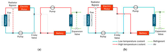
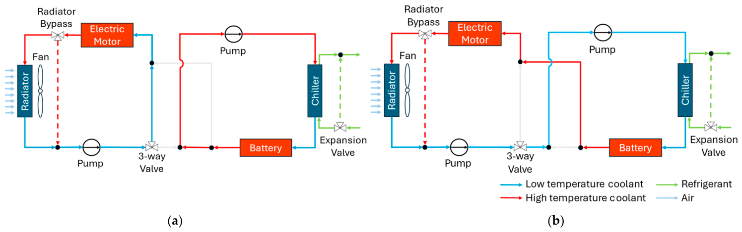
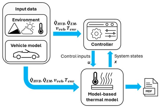
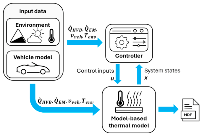
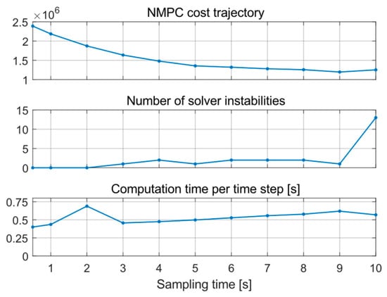
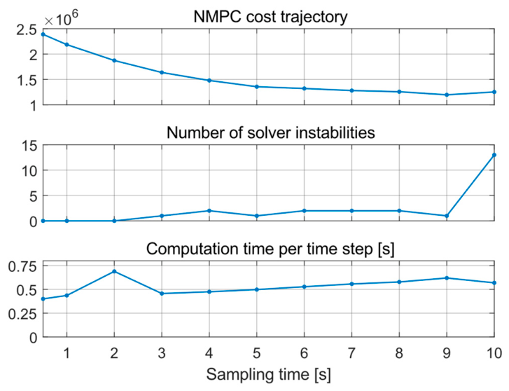
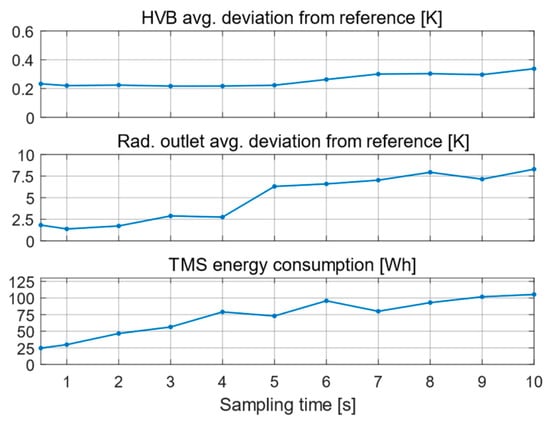
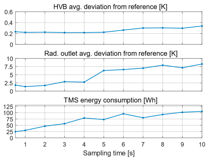
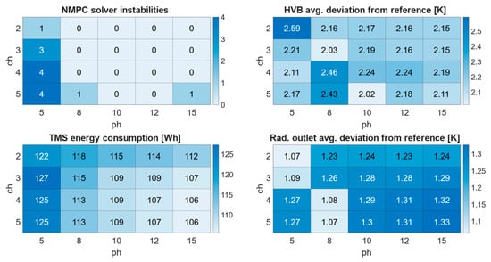
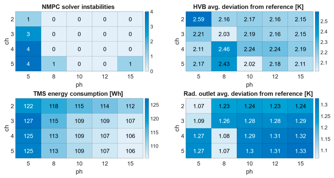
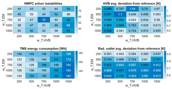
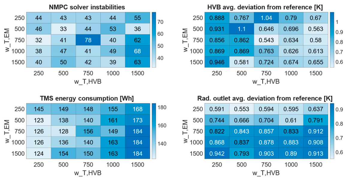
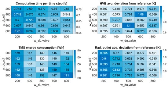
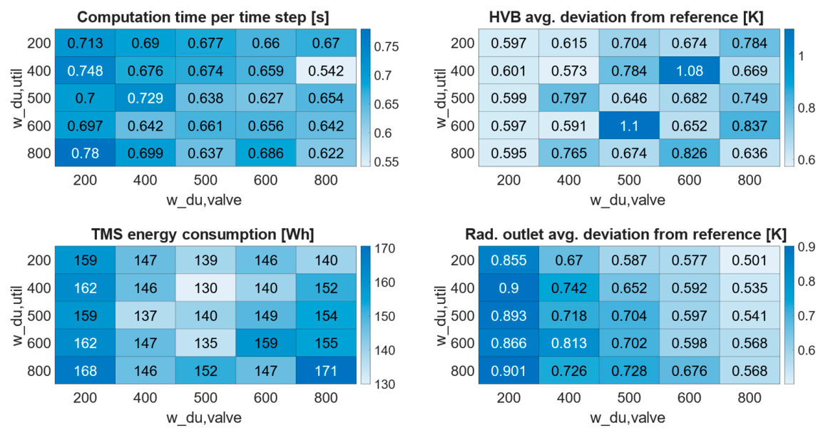
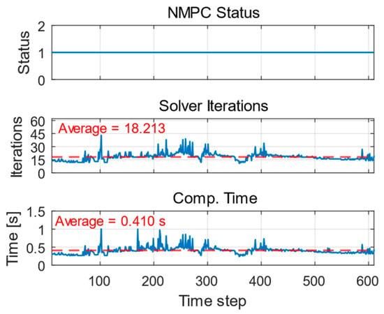
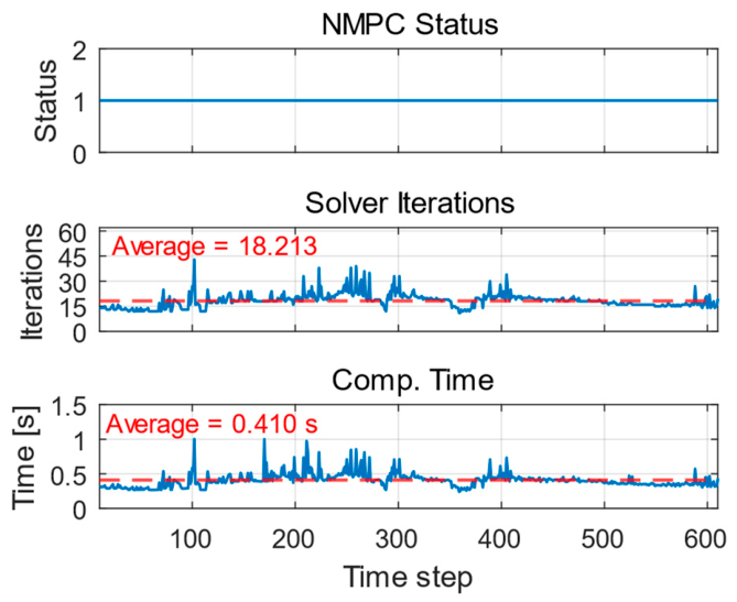
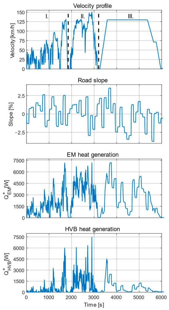
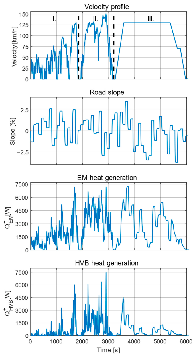
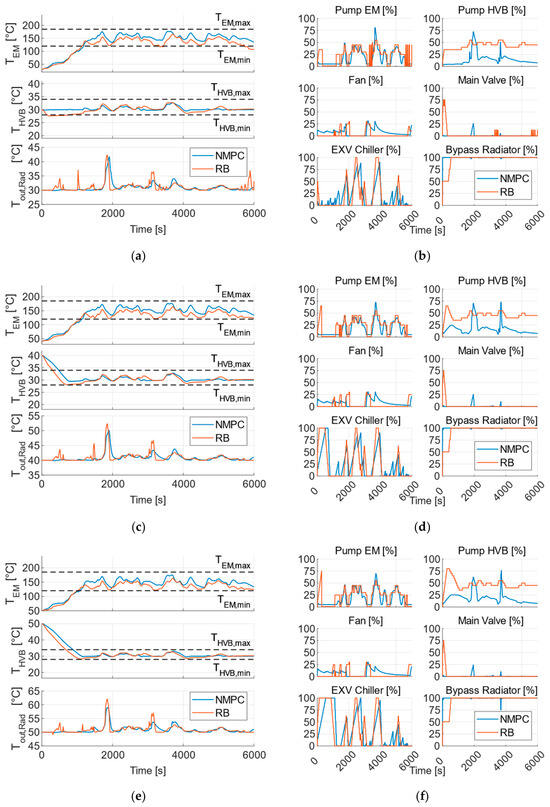
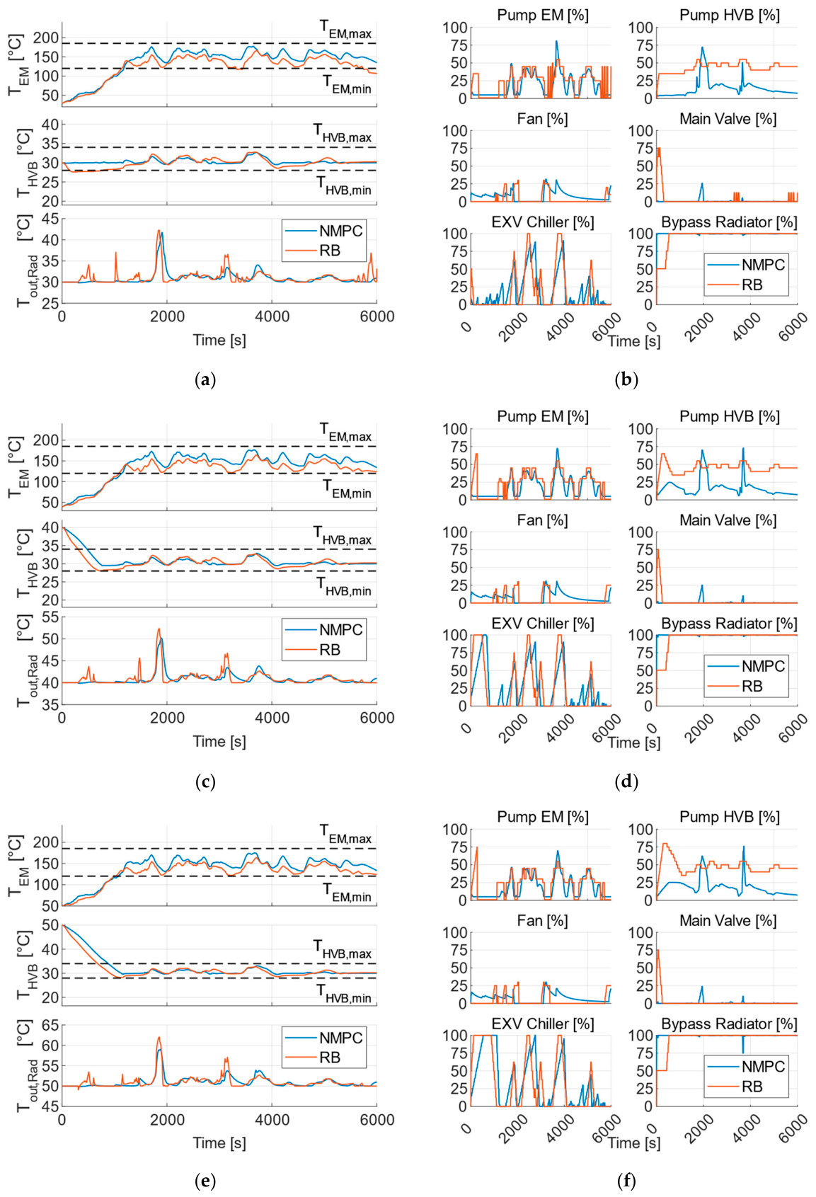
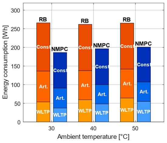
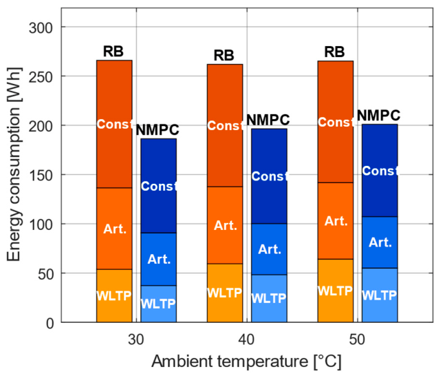
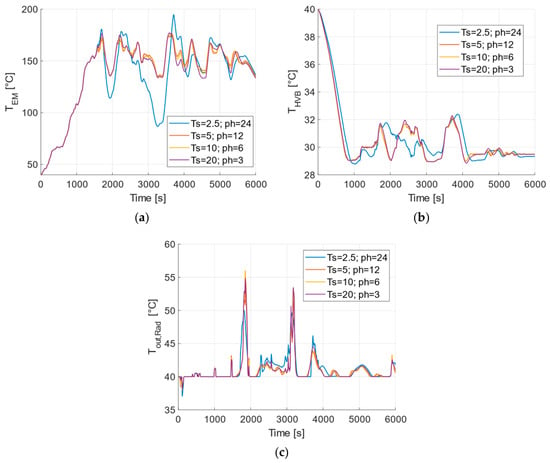
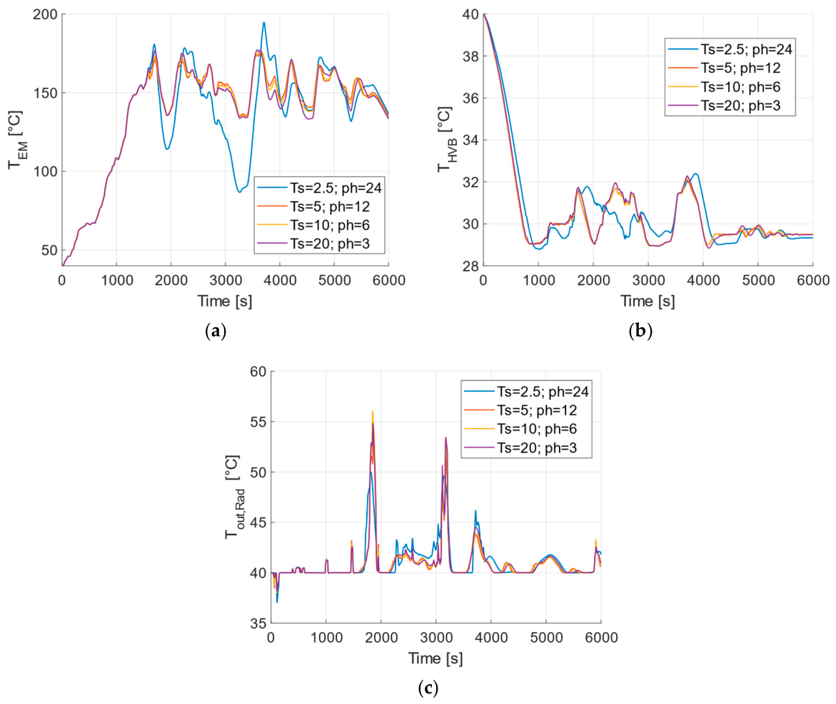
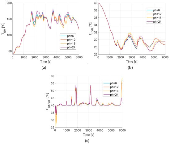
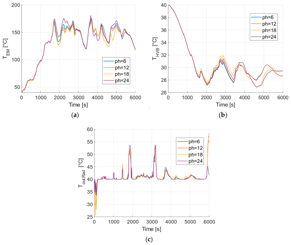

Disclaimer/Publisher’s Note: The statements, opinions and data contained in all publications are solely those of the individual author(s) and contributor(s) and not of MDPI and/or the editor(s). MDPI and/or the editor(s) disclaim responsibility for any injury to people or property resulting from any ideas, methods, instructions or products referred to in the content. |
© 2026 by the authors. Published by MDPI on behalf of the World Electric Vehicle Association. Licensee MDPI, Basel, Switzerland. This article is an open access article distributed under the terms and conditions of the Creative Commons Attribution (CC BY) license.