


Highlights
What are the main findings?
- A physics-informed multi-objective genetic algorithm (NSGA-II, an evolutionary AI method) coupled with 2D finite-element evaluation was applied in two stages to Fe, Me and Vi at 85 kHz. In the first stage (10 kW), the analytical power density differed from the FEMM-validated value by 73.7% (Fe), 22.7% (Vi) and 11.4% (Me), so the analytical sizing is conservative; in the second, independent stage (22 kW, five seeds per material), the finite-element model raised the total loss by a median of 3–11%, lowered the leakage inductance by about 48% and exposed a winding hotspot about four times the lumped rise, which excludes 31–54% of the designs under a 100 K limit.
- In the first stage, Vi gave the best efficiency–compactness balance (11.84 W/cm3 FEMM-validated at a simulated peak transformer-only efficiency of 99.46%, with a broad search indicating up to 61.2 W/cm3 before thermal and manufacturing constraints); in the second stage, Fe and Vi reach 6–37 and 7–27 W/cm3 at 99.8–99.9% efficiency and Me 5–9 W/cm3, limited by its loss at 85 kHz. The Fe–Vi ranking depends on the loss fits, the cooling coefficient and the temperature limit, and all results are simulated.
What are the implications of the main findings?
- Replacing the uniform-flux and lumped-thermal assumptions by field and heat-conduction solutions reveals flux crowding, skin and proximity effects and a winding hotspot that analytical models cannot capture, and the Litz optimisation (AWG 44–46 single-strand windings with an AC-to-DC inflation factor below 3.0; AWG 38–42 transposed double-strand bundles with 1.08–1.16) is consistent with the finest-strand designs selected by the second-stage search.
- The module-level ranking is independent of the ISOS, IPOS, ISOP or IPOP arrangement, so the pairing of Vi with ISOP stages and Me with IPOP stages is retained as indicative guidance; a closed-loop dual-active-bridge simulation with the extracted inductance and a controller designed for a 55° phase margin shows soft switching and a well-damped current loop, pending prototype and three-dimensional thermal validation.
Abstract
Integrating electric vehicles (EVs) into power grids requires efficient, compact high-frequency transformers (HFTs) for solid-state-transformers (SST) and charging stages. This paper combines a physics-informed multi-objective genetic algorithm (NSGA-II, an evolutionary AI method), two-dimensional finite-element (FE) evaluation and dual-active-bridge (DAB) simulation to size HFTs at 85 kHz for ferrite 3C94 (Fe), Metglas 2605SA1 (Me) and Vitroperm 500F (Vi). In a first, FEMM-based stage (10 kW), analytical power density differed from FEMM by 73.7% (Fe), 22.7% (Vi) and 11.4% (Me); Vi reached 11.84 W/cm3 at a simulated peak transformer-only efficiency of 99.46%, and Litz optimisation identified AWG 44–46 and AWG 38–42 operating points. A second, independent stage (22 kW, five seeds per material) shows that the FE model raises the total loss by 3–11%, lowers the leakage inductance by about 48% and reveals hotspots about four times the lumped rise, excluding 31–54% of the designs at a 100 K limit. Fe and Vi then reach 6–37 and 7–27 W/cm3 at 99.8–99.9% efficiency and Me 5–9 W/cm3, and a designed DAB current loop is well damped (55° phase margin). The ranking is sensitive to loss fits and cooling prediction.
1. Introduction
The global effort to reduce GHG emissions has accelerated the transition of the transportation sector from internal combustion engine vehicles (ICEVs) toward electrified mobility [1,2]. Although EVs can reduce dependence on petroleum-based transportation, their practical performance is strongly influenced by the efficiency of the electric drivetrain, the usable energy capacity of the battery pack and the operating conditions imposed by the vehicle drive cycle [3,4]. These factors directly affect charging demand, energy consumption and driving range. Consequently, improving charging infrastructure is essential for supporting the large-scale deployment of EVs [5,6].
Both static and dynamic charging of EVs need reliable, high-quality power. While static charging involves charging a stationary EV or hybrid EV, Dynamic Wireless Power Transfer (DWPT) has emerged as a promising approach for reducing the range limitations associated with battery-powered transportation, even as the car is in motion or partially in motion (quasi-static) [7,8]. Unlike conventional plug-in charging, DWPT transfers electrical energy to a moving vehicle through magnetic coupling between a roadway-mounted transmitter and a receiver installed beneath the vehicle [9,10]. A representative DWPT system is illustrated in Figure 1.
Figure 1.
DWPT system.
The primary-side power-conversion chain generally consists of an AC–DC rectifier, a power-factor-correction (PFC) stage, and a HF inverter [11,12,13]. The rectifier and PFC stage establish a regulated DC-Link (DCL) and shape the grid current, whereas the inverter converts the DCL voltage into a HF excitation waveform for the transmitting pad [14,15]. On the vehicle side, the receiving pad captures the transferred HF electromagnetic power and supplies it to a compensation and conversion system [16,17]. Depending on the selected architecture, this system may include a resonant compensation network, a HF rectifier, an isolated DC–DC converter, and battery-charging control [18]. These stages regulate the voltage and current delivered to the EV battery while maintaining galvanic isolation and accommodating variations in coupling coefficient, air gap, vehicle position, and battery operating point [19]. Figure 1 should be interpreted as a representative conversion architecture rather than a universal circuit configuration [20].
The High Frequency Transformer (HFT) is a key isolation and energy-transfer component in the proposed conversion system. HFT is the Solid-State Transformer (SST) core, while the DC–DC (like the Dual Active Bridge (DAB)) converter unit is the SST central processing unit. It should be distinguished from a complete Power Electronic Transformer (PET) or SST. While the HFT provides HF galvanic isolation and voltage transformation, the PET/SST comprises the HFT together with the associated semiconductor converters, control system and auxiliary components. The SST structural classification matrix, types, conversion stages, PFC system, DCLs, bidirectional capability, efficiency and relative cost trend are detailed in Figure 2.
Figure 2.
PET types (a) PET conversion stages, (b) topology matrix and (c) efficiency vs. relative production cost model.
Role of the HFT in the charging chain. The closed-core HFT designed here is the isolation and voltage-transformation element of the DC–DC stage (DAB/LLC) of an SST-based or on-board charger. Its magnetic circuit is closed and tightly coupled, so that core loss, saturation margin, winding loss, leakage inductance and insulation dominate the design. This differs from the loosely coupled transmitter/receiver coil pair of a wireless power transfer (WPT) system (Figure 1), where leakage, compensation and pad geometry dominate. The frequency of 85 kHz is the nominal SAE J2954 value, so the results apply to converter stages feeding J2954-class pads, not to the coupler.
Terminology used in the title. “AI-assisted” denotes the evolutionary multi-objective search (a branch of artificial intelligence) combined with physics-based models; no learned surrogate is used. “Dynamic validation” denotes the check of the field-derived transformer inductance in a switching-cycle and closed-loop model of the dual-active-bridge (DAB) stage (steady-state waveforms, soft-switching region, and the response of a current controller to a reference step and an input-voltage dip, Section 3.6); it does not include a prototype test. “High-efficiency” refers to the transformer-only efficiency. The HFT is the SST module (ISOS, IPOS, ISOP, IPOP) whose isolation core is designed.
Compared with a conventional Low or Line Frequency Transformer (LFT), HFT can provide substantially greater power density because its higher operating frequency permits a reduction in magnetic-core cross-sectional area and winding volume [21]. When integrated with controlled power electronic stages, the resulting PET/SST platform can also support bidirectional power transfer, voltage regulation, reactive-power management, power-quality improvement and controlled fault response, as modelled in Figure 2. These benefits are accompanied by significant design challenges. Increasing the switching frequency reduces the size of the magnetic components but can increase core loss, winding loss, proximity and skin effects, electromagnetic interference and semiconductor switching loss; in addition, the selection of appropriate magnetic material involves a compromise among core-loss density, saturation flux density, manufacturability (including parameter value differences or discrepancies), thermal performance, insulation requirements and material cost [22]. These trade-offs become more pronounced in WPT applications because the transformer must operate efficiently under variable frequency, load and magnetic-coupling conditions [23].
Related work. WPT for EVs covers static and dynamic inductive charging [7,8,9,10,13,14], multi-coil and scalable arrays [12,17], and free-moving transmitter arrays tolerant to receiver orientation [24]. At higher power, SST-based ultra-fast charging stations rely on modular isolation stages whose efficiency, thermal reliability and modularity are central design drivers [25]. Within HFT design, existing work optimises one material class or winding type, for example a nanocrystalline HFT with multi-physical-field modelling [22], copper-foil versus Litz windings [26], Litz windings in SSTs [27] and 2D finite-element Litz AC resistance [28]; genetic-algorithm and Multiphysics HFT design is reported in [29,30,31], thermal design for DAB converters in [32], NSGA-II [33] is the usual search engine, and AI in magnetic design is surveyed in [23]. Still missing is a like-for-like comparison of the main soft-magnetic families under one constraint set that also quantifies how far lumped analytical models depart from field-based evaluation of loss, leakage inductance and hotspot temperature, and that reports the convergence and diversity of the search.
To address this gap, this paper develops an AI-assisted, physics-informed multi-objective genetic algorithm (MOGA) for HFT design. The AI component is an evolutionary multi-objective search (NSGA-II with constraint domination), not a learned surrogate. The contributions are: (i) a seven-variable real-coded design vector (core leg width and depth, window height and width, turns, current density and Litz strand gauge) evaluated with iGSE core loss, strand-level Litz loss, a window-based leakage-inductance model, a lumped thermal model and an explicit cost model; (ii) two-dimensional finite-element re-evaluation of the Pareto set for local flux density, core and proximity loss, leakage inductance and the winding hotspot, from which a hotspot criterion re-sorts the designs; (iii) a like-for-like comparison of ferrite 3C94 (Fe), Metglas 2605SA1 (Me) and Vitroperm 500F (Vi) under one 22 kW, 85 kHz design basis with five independent runs per material, hypervolume and diversity monitoring and sensitivity analyses; (iv) a closed-loop DAB check that uses the extracted leakage inductance; and (v) the retention of the first-stage FEMM-based results of earlier work [34,35,36], with their figures and tables, which are reconciled with the new results (Section 3.7 and Section 3.8). The paper presents the models and optimisation (Section 2), the results (Section 3), the EV integration discussion (Section 4) and the conclusions (Section 5).
The four modular configurations, Input-Series Output-Series (ISOS), Input-Parallel Output-Series (IPOS), Input-Series Output-Parallel (ISOP) and Input-Parallel Output-Parallel (IPOP), differ in how the voltage and current are divided among identical modules. The HFT is therefore designed at module level under one common power rating, frequency and constraint set, and the topology then determines the per-module voltage, current and insulation stress (Section 2.4). The four configurations are not optimised separately.
2. Materials and Methods
2.1. Analytical Design and Electro-Thermal Optimisation of HFT
The analytical design of HFTs within EV and SST architecture necessitates a multi-physics co-design framework that simultaneously satisfies electromagnetic, thermal and geometric constraints [27]. Because preliminary sizing involves non-linear interdependencies between core cross-sectional geometry, window utilisation factor and thermal dissipation boundaries, iterative design loops must be anchored by rigorous optimisation criteria. To establish an optimal operating point that balances core losses against copper heat losses while preventing thermal degradation, the peak magnetic flux density is formulated in (1) [28].
where denotes the conductor resistivity, represents the convective heat transfer coefficient governing surface thermal dissipation, and define the window utilisation and copper fill factors and signifies the allowable core-to-ambient temperature rise. The topology-dependent dimensionless coefficients and characterise core geometry (with standard empirical benchmarks of , and ). Additionally, denotes the aggregate apparent power rating, is the excitation waveform factor ( for sinusoidal and for bipolar square-wave excitation), is the core stacking factor and is the Steinmetz core loss exponent. Equation (1) provides a robust deterministic baseline for initial core sizing. HF operation introduces severe parasitic phenomena, including HF fringing fields, eddy current losses, skin and proximity effects in conductors and complex core loss accumulation under non-sinusoidal Pulse-Width Modulated (PWM) voltages. Consequently, this analytical sizing model serves as the foundational initialisation layer for advanced multi-objective Pareto optimisation, ensuring that thermal equilibrium and magnetic saturation margins are systematically maintained prior to detailed finite element verification. To translate the optimal magnetic flux density into physical core dimensions, the core area product () formulation, bridges geometric utilisation with electrical and thermal constraints. The required core area product is expressed in (2) [26].
where the auxiliary thermal-geometric coefficient is defined in (3).
To account for the total power processed through the HF transformer windings relative to the converter conversion efficiency () and nominal output power (), the aggregate apparent power rating () is formulated in (4).
This analytical framework enables systematic sizing of the magnetic core, establishing a rigorous mathematical bridge between preliminary volumetric estimation and detailed finite-element thermal-magnetic validation.
2.2. Volumetric Co-Design, Core Loss Modelling and Hf Winding Optimisation
Balancing volumetric power density with thermal efficiency is a fundamental trade-off in HFT design. While minimizing core volume maximises power density, it often exacerbates flux density crowding and thermal bottlenecks. The respective core and winding volumes are defined geometrically (5) and (6).
where denotes the mean magnetic path length of the core, is the mean length of a turn and and represent the core cross-sectional area and overall winding cross-sectional area, respectively.
2.2.1. Core Loss Estimation via Improved Generalised Steinmetz Equation (iGSE)
Under non-sinusoidal voltage excitation typical of PET converters, conventional Steinmetz formulations underestimate magnetic losses. To accurately capture HF dynamic core losses, the iGSE is implemented in (7) and (8) [26].
where the waveform-dependent coefficient is formulated as:
Here, represents the switching period, is the peak-to-peak flux density variation, and , and (or ) denote the material-specific Steinmetz coefficients fitted to published loss data for the same material classes, as listed in Table 1 (see Section 2.4).
Table 1.
Steinmetz coefficients for soft-magnetic core materials.
Flux-density waveform. In the DAB/LLC stage the HFT is excited by a bipolar, approximately rectangular voltage (with an approximately sinusoidal current near resonance). The core flux density follows Faraday’s law, , so a symmetric two-level square wave of amplitude produces a triangular flux density with peak and peak-to-peak excursion . This is inserted in (7), so that the dependence of loss on the actual , rather than on a sinusoid of equal amplitude, is captured. In the finite-element stage (Section 2.7) the magnetostatic solution provides the spatial distribution of the flux-density amplitude, from which the local peak and the leg average are taken.
Minor loops, DC bias and waveform effects. For steady-state, volt-second-balanced operation the flux follows one symmetric loop per period, so no minor loops arise and the iGSE is a single-loop evaluation. DC bias is taken as zero because the series capacitor of the LLC-DAB stage blocks DC; a residual bias would reduce the saturation margin and is not modelled. Not included are relaxation effects (i2GSE), the temperature dependence of the Steinmetz coefficients (Table 1), stress-induced loss increase in cut or encapsulated ribbon cores and the DC-bias dependence of Fe loss, so the core-loss uncertainty is that of the datasheet fit and should be confirmed by measurement.
2.2.2. High-Voltage (HV) Insulation Coordination
In Medium-Voltage (MV) SST applications, galvanic isolation between primary and secondary windings requires strict adherence to clearance standards. The minimum insulation thickness () is determined by using (9) [37]
is the required isolation voltage rating, represents the dielectric breakdown strength of the selected insulation medium and is an empirical safety margin specified by design standards.
2.2.3. Analytical Formulation for HFT Winding AC Resistance and Thermal-Current Optimisation
Litz Wire Packing Factor and Optimum Strand Sizing
Litz wire is the standard for HFT, with empirical packing factor () models conductor fill efficiency as a function of uninsulated strand diameter [38] is modelled in (10).
The analytical optimum strand diameter () that minimises total HF copper losses (balancing skin and proximity effects) is solved via (11) [39].
is an auxiliary geometry factor incorporating layer count () and bundle packing () and is given in (12).
The non-dimensional skin-to-bundle transformation parameter () is expressed in (13) [40]:
Truncated Dowell Auxiliary Functions and AC Resistance Modelling
To replace computationally heavy Kelvin/hyperbolic functions () during optimisation, the orthogonality functions and are expanded via Taylor series (14) to (15).
Combining these auxiliary functions yields the absolute HF AC resistance () of the Litz winding using analytical dimensional parameters, including the Litz-wire packing factor (), number of winding layers () and strand count per conductor () as shown (16).
For simplified round solid conductors (non-Litz), the HF AC-to-DC resistance ratio () is approximated using the empirical polynomial model in (17).
Equation (18) represents the physical conductor radius relative to the electromagnetic skin depth () of the copper at the operating switching frequency. At high switching frequencies, skin and proximity effects severely increase conductor AC resistance compared to its DC baseline. is a function of the switching frequency , copper conductivity and permeability of free space as depicted in (19).
Total Litz Winding Losses and Thermal-Current Coupling
Total transformer Litz wire winding loss () combines primary () and secondary () RMS currents and AC resistances in (20).
Using structural volume-based optimisation, winding loss is computed over winding sections and area ) as depicted in (21).
The maximum allowable current density () coupled with core thermal dissipation limits () and Steinmetz core parameters () is expressed in (22).
The optimised Litz wire has multi bundled strands twisted turns (Ns), outer jacket or serving insulation, and single strand enamel insulation film layer enclosing pure copper conductor with single strand diameter that is less than twice the skin depth ). The design algorithm is depicted in Figure 3.
Figure 3.
Litz wire Optimisation algorithm.
2.3. Physics-Based Multi-Objective Optimisation
The analytical approaches for electromagnetic field and temperature distribution analysis become difficult for HFTs; numerical approaches such as multi-objective optimisation coupled with finite-element analysis are therefore used [23]. In this study the optimisation, the finite-element solutions and the DAB simulation are implemented in Python 3.15.2. (pymoo (multi-objective optimization in Python) 0.6.2. [41] for NSGA-II, scikit-fem 12.0.2 [42] for the finite-element solutions). The governing partial differential equation of the 2D quasi-static magnetic model for the magnetic vector potential is given in (23); the 2D steady heat-conduction problem used for the hotspot is stated in Section 2.7.
where is the magnetic reluctivity (), is the magnetic vector potential (), is the eddy current density (), ∇ is the curl operator representing a standard vector calculus mathematical operator, is the imaginary unit ( representing the complex phasor domain, is the frequency in , and is the electrical conductivity (). This study uses the NSGA-II search, with the finite-element solutions of Section 2.7, to optimise three key HFT design objectives: total loss, power density (volume) and material cost. This process identifies the most suitable soft magnetic material for each HFT application considered.
2.3.1. Multi Objective Design Optimisation
The optimisation objectives are discussed below.
The Total Power Loss
Eddy current and hysteresis losses increase dramatically at high frequencies. In addition, the skin effect also has a greater influence; however, this can be readily resolved by employing Litz wires for the HFT’s windings [43]. As described in (24), the approximate total losses, , in the HFT is the sum of the core losses (hysteresis and eddy current ) and the copper winding losses ). and are retrieved from (25) and (26).
If (25) is expressed relative to core mass in (26), then instead of (25), (27) generates . are retrieved from (20) and (22).
is the electrical resistivity of the winding material, is the mass density of core material, is the maximum flux density, are the core loss parameters.
Scope of the efficiency figure. The efficiency used throughout is the transformer-only efficiency , with from (24); it counts only the core and winding losses of the HFT and is the quantity constrained in (32). It excludes semiconductor conduction and switching losses, rectifier, resonant-tank (capacitor and external inductor), coil-pad, cable and auxiliary losses, and must not be read as the efficiency of the SST or of the wireless-charging system. A system-level figure would have to add these terms.
Power Density (PD)
The volume of transformers can be greatly reduced at higher frequencies. In EV, since weight is an important factor, a compact HFT with high power density is desirable. The optimisation of the HFT’s size is interpreted as optimisation of the weight and volume of the SST core architecture. Power density, in , is calculated using (29).
where and are the core and winding-bundle volumes defined in (5) and (6) and evaluated with the design vector of Section 2.5 (Equation (44)).
is HFT’s output power, are the height, length, thickness and core build of the HFT core, respectively, while are the HFT core window height and width all in . The core and winding model are shown in Figure 4a and Figure 4b, respectively.
Figure 4.
The (a) core and (b) winding design.
Definition and scope of the power density. in (29) is an active-volume power density: the output power divided by the volume of the magnetic core plus the volume of the winding bundle (Litz cross-section including the strand enamel and the insulation allowance through the packing factor ). It does not include the winding-to-core clearances, the bobbin or former, encapsulation, mechanical supports and clamps, terminations or the thermal-management system (heat sinks, fans, cold plates or potting). The reported values are therefore upper bounds on the packaged power density. If these items add a fraction of the active volume, the packaged value is ; for the illustrative range – the values reported in Section 3 are divided by 1.2–1.5. Numerically, 1 W/cm3 equals 1 kW/L.
The Total Cost
The HFT’s cost is also a key consideration for optimisation, the price of Litz wire and the different core materials, namely (Fe (3C94), Amorphous (Me) and Nanocrystalline (Vi)) make up the cost of each HFT design. The total cost of the HFT is expressed in (31).
where , , and are number of primary turns, number of secondary turns, cost coefficients of the Litz wire and cost coefficients of the core materials used, respectively.
2.3.2. Design Optimisation Constraints
To bound the feasible solution space and guarantee physical realisability within the multi-objective optimisation framework, a rigorous set of operational, geometric and converter-level constraints is formulated. These constraints govern the HF transformer (HFT) efficiency, the HFT core in Figure 5a, the core dimensional limits in Figure 5b and power electronic converter compatibility.
Figure 5.
3D Representation of the (a) HFT Core with (b) Optimisation Dimensions.
Efficiency Constraint
The operating efficiency of the HFT must satisfy or exceed the minimum threshold specified by converter design requirements, defined as and modelled in (32).
Core Dimensional Constraints
To ensure that optimised dimensions translate into manufacturable hardware, the upper bounds corresponding to baseline core dimensions () are enforced across the core height (), length (), depth (), and centre limb width () as modelled in (33).
Power Electronic Converter and Quality Factor Constraints
For PET-EV applications, the DAB topology uses an Inductor-Inductor-Capacitor (LLC) resonant network (and the equivalent circuit) shown in Figure 6 and Figure 7, due to its high voltage regulation capabilities and soft-switching performance within wide load variations. The frequency-domain voltage transfer function of the LLC-DAB converter is modelled and expressed from (34) to (39).
where the total primary-side leakage inductance is defined as:
Figure 6.
DAB topology incorporating an LLC resonant network.
Figure 7.
DAB LLC equivalent resonant network circuit.
The inductive parameters are extracted from the 2D field solution. The model depth is the stack depth , so that each surface integral over the 2D cross-section is converted to a volume integral by multiplying by . Energising only the primary with A gives the primary self-inductance ; energising only the secondary with A gives . With both windings energised by unit currents in the flux-aiding direction the integral equals twice the stored energy, , so the mutual inductance is obtained from half of the difference (the cross term appears twice):
The mutual inductance is not itself the excitation-branch inductance of the equivalent circuit in Figure 7. With the turns ratio , the T-equivalent circuit referred to the primary has the magnetising inductance, primary-side leakage inductance and secondary-side leakage inductance (not referred) given by:
In (34)–(35), is therefore the magnetising inductance of the primary-referred T-model, and are the primary-side and secondary-side leakage inductances (so that is the secondary leakage referred to the primary), and adds the external resonant inductance . Equation (39) defines the total leakage inductance from the stored field energy with the secondary short-circuited at primary current ; the factor 2 follows from , and (39a) shows its equivalence with the T-model parameters. In the present study, only of (39) is extracted from a balanced short-circuit solution (Section 2.7); , and are not needed at module level. The 2D model neglects end-winding and fringing contributions to the leakage inductance, which a 3D model or an end-turn correction would add.
To achieve zero-voltage switching (ZVS) and zero-current switching (ZCS) across loading conditions, the resonant circuit quality factor is constrained within the range shown in (40) when the LLC network is used. The module-level optimisation of this paper does not enforce (40); it bounds the leakage inductance by the power-transfer limit of the DAB (Section 2.4) and checks soft switching directly in the DAB model of Section 2.8.
2.4. Design Basis, Materials and Topology Scaling
All three materials are optimised under one design basis for a single HFT module: output power kW, operating frequency 85 kHz, a symmetric bipolar rectangular winding voltage of V from the DAB bridges (an 800 V EV battery architecture, 1:1 turns ratio) and a design winding current A rms. The factor 1.10 covers the non-sinusoidal DAB current: for the total inductance of 20 µH used in Section 3.6 the rms inductor current is within 1% of this value. The thermal budget is a lumped temperature rise of at most 60 K above ambient with a surface heat-transfer coefficient W/(m2·K) (forced air), a winding temperature of 100 °C for the copper resistivity, an insulation distance for kV with a dielectric field of 15 kV/mm and a safety margin of 3 (Equation (9)), a minimum winding-to-winding gap of 1 mm and a minimum transformer-only efficiency . The leakage inductance is bounded above by µH, which is 91% of the value µH at which the single-phase-shift DAB transfers at the maximum phase shift. The peak flux density is limited to 80% of the saturation induction . [Authors: confirm the design basis (22 kW, 800 V, 85 kHz) and insert any project-specific insulation class and ambient temperature.]
Because each module of an -module ISOS, IPOS, ISOP or IPOP system processes at the same frequency, the core and winding optimisation at module level, and therefore the material ranking of Section 3, does not depend on the topology. The topology changes the per-module voltage and current (Table 2) and hence the turns ratio, insulation and conductor sizing. The four configurations are therefore compared through Table 2 and Section 4 rather than through four separate optimisations.
Table 2.
Per-module quantities of the four modular configurations for identical modules (ideal, equal sharing, ).
The three materials represent the soft-magnetic families usable at tens to a few hundred kHz and span the main trade-offs among saturation induction, loss, cost and manufacturability (Table 3): Fe is the low-cost, high-resistivity reference with standard geometries; Me is an iron-based amorphous ribbon with the highest saturation induction; Vi is a nanocrystalline ribbon with high permeability and low specific loss at high frequency. The core loss is described by the Steinmetz fit of Table 1, converted to the iGSE coefficient of (8) for the triangular flux of a square-wave voltage. The fits are literature fits of the same material classes (per unit volume for Fe, per unit mass for the ribbons), valid near 100 °C; the Me fit is extrapolated to 85 kHz and the Vi fit is a published nanocrystalline fit used as a proxy for the 500F grade, so the loss comparison inherits their uncertainty and is explored in Section 3.5 [44,45,46].
Table 3.
Candidate core materials, properties used in the optimisation and selection rationale.
2.5. Candidate Evaluation Model
Each candidate is a design vector of the leg width (), the stack depth (), the window height and width (), the number of turns per winding, the current density and the Litz strand gauge index (AWG 38, 40, 42, 44 or 46). The core height and length are and . Table 4 gives the bounds. With the effective core cross-section ( the stacking factor), Faraday’s law for the square-wave voltage gives the peak flux density, and the iGSE [47] of (7)–(8) gives the core loss density for the resulting triangular flux:
Table 4.
Design variables, bounds and encoding of the optimisation (real-coded; the strand gauge is rounded to the nearest listed AWG).
The core loss is for Fe and for the ribbon cores, with the core volume and the mean path length . The winding is a Litz bundle of strands of area and packing factor (including enamel and serving insulation). The direct-current and strand-level proximity losses [48] of the two windings are given in (42).
where is the mean turn length, the usable window height ( mm clearance), the copper resistivity at 100 °C and the factor is the mean-square value of the transverse field across a winding with a linear field profile; the skin effect within a strand is negligible because every strand is thinner than the skin depth (about 0.26 mm at 85 kHz and 100 °C). The leakage inductance referred to the primary, the total loss, the lumped temperature rise and the objectives are
with the winding builds, the insulation gap of (9) and the surface of the bounding box of the core and windings. The three objectives are the total loss , the active volume (core plus winding bundle, which is the reciprocal of the power density (29)) and the cost , with core mass priced by Table 3 and copper at 0.35 USD/cm3 of copper volume (the prices of Table 3 are, therefore, assumptions, not quotations; Section 3.5 varies them). The constraints, written as , are: ; K; the winding build including the gap and clearances within the window width; the window fill ; µH; with from the loss of (24) and a minimum window width. The problem is
2.6. Multi-Objective Genetic Algorithm and Convergence Indicators
The search uses the elitist non-dominated sorting genetic algorithm NSGA-II [33] with constraint domination (a feasible design dominates an infeasible one; between infeasible designs the smaller total violation wins), implemented in pymoo 0.6.2 [41]. The decision vector is real-coded, and the variation operators are simulated binary crossover [49] (probability 0.9, distribution index ) and polynomial mutation (distribution index , probability per variable). The population size is 100 and each run lasts 250 generations (25,000 candidate evaluations). Each material is run with five independent random seeds (0–4). Crowding-distance sorting preserves the spread of the front.
Two indicators are recorded each generation . The hypervolume [50] of the feasible non-dominated set is computed in the objective space normalised by the fixed reference point , so that . The decision-space diversity is the mean pairwise distance of the population in the normalised variables :
with and . Premature convergence is flagged when collapses while is still increasing, and stagnation at a poor front when is flat while remains high. As a check against local minima, the final hypervolumes of the five seeds are compared through their mean and standard deviation, and the seed with the largest hypervolume is used for the finite-element stage. Selecting that seed is a choice and slightly favours the reported front; the spread across seeds is reported with it.
2.7. Two-Dimensional Finite-Element Re-Evaluation
Each of the 100 non-dominated designs of the selected seed is re-evaluated with a 2D finite-element model in the plane of the window (scikit-fem [42], bilinear quadrilateral elements on a tensor-product mesh with the interfaces of the core, the four winding blocks and the air padding on mesh lines; the stack depth is the out-of-plane length). Two magnetostatic solves of with on a padded outer boundary are performed with linear relative permeabilities of 3000 (Fe), 8000 (Me) and 20,000 (Vi): (i) a balanced short-circuit excitation (primary and secondary ampere-turns opposed in the window) for the leakage inductance with the stored energy times the depth, and for the local transverse field in the windings, from which the proximity loss of (42) is integrated element-wise; (ii) a magnetising excitation, whose core flux-density distribution is scaled so that its mean in the leg equals of (41), from which the local iGSE loss density is integrated over the core. The ratio of the 99.5th-percentile local flux density to is the flux-crowding factor (the extreme inner-corner singularity is excluded). The saturation limit is checked on the 99.5th percentile.
Hotspot model. The steady heat-conduction problem is solved on the window cross-section with the heat sources from the local core iGSE loss density and the winding spread uniformly over the winding blocks, thermal conductivities of 4 (Fe) and 3 W/(m·K) (ribbon cores, through-stack equivalent), 1.0 W/(m·K) for the Litz bundles and 0.026 for air, and a convective condition on the outer boundary. The surface coefficient of the slice is chosen so that the slice rejects its heat at the same mean surface rise as the lumped model, (an energy-consistent calibration, because the 2D slice has no fringing surface). The hotspot rise is the maximum of the solution, and the extra rise over the lumped value of (43) therefore measures the conduction resistance inside the bundle and the core, which the lumped model neglects. A limit K is applied to the finite-element set (winding hotspot of about 140 °C at 40 °C ambient, below the 155 °C of an insulation class F). [Authors: replace the assumed conductivities by measured or datasheet values if available.]
Mesh convergence and three-dimensional thermal check. The element size is the smallest of the leg width, window height and winding build divided by 3.5 (at least 0.4 mm). Refining the elements by a factor of 0.5 (about three times as many elements) for the first, fifth and tenth design of each material changes the leakage inductance by at most 1.1%, the finite-element core loss by at most 0.3%, the proximity loss by at most 1.3% and the 99.5th-percentile flux density by at most 8% (the inner-corner value), so the baseline mesh is used. Reviewers asked for a three-dimensional heat-transfer analysis; for the fourth and seventh design of each material the same heat sources are therefore extruded into a three-dimensional hexahedral model (stack depth ; the winding blocks extend by one winding build beyond both ends of the stack to represent the end turns; uniform heat density in the windings; the same conductivities) with the convective condition W/(m2·K) applied to the whole outer surface of the bounding box, without any calibration. This is a conduction model with a prescribed surface coefficient and not a conjugate fluid–thermal simulation.
2.8. Dual-Active-Bridge Model for the Dynamic Check
The DAB is modelled with single-phase-shift modulation, , with the series inductance (the finite-element leakage of the selected design plus an external inductor), V and a battery of open-circuit voltage 760 V and resistance 0.8 Ω behind a 470 µF output capacitor. The transferred power is [51], and the inductor current is computed in the time domain over one switching period to obtain the steady-state waveforms, the rms and peak currents and the soft-switching region (the inductor current at the first bridge-leg switching instants has to discharge the switch capacitances, which is tested through its sign at the two switching instants). A cycle-averaged model is used for the current loop. Around the rated point the battery current responds to the phase shift as with A and µs. The controller is a PI regulator sampled at 10 kHz, with a computation and hold delay of 1.5 samples and a 5 kHz current-sensor filter. Its zero cancels the plant pole () and its crossover is the highest value that leaves a phase margin of at least 55° (530 Hz), which gives and (per-unit phase shift per ampere and per ampere-second). Conditional integration provides anti-windup, and the controller output is scaled by because the transferred current is proportional to . The design is verified for a reference step (50% to 100% of the rated 27.5 A) and an input-voltage dip of 5%. The total inductance is set to µH, which gives a rated phase shift .
3. Results
The results are obtained with the models and settings of Section 2. Figure 8 shows the workflow. Unless stated otherwise, “finite element” (FE) refers to the 2D re-evaluation of Section 2.7, and the quantities are for the best seed of each material.
Figure 8.
Workflow of the study: NSGA-II search with analytical evaluation, finite-element re-evaluation and hotspot filtering of the Pareto set, closed-loop DAB check and sensitivity analysis.
3.1. Convergence, Diversity and Repeatability of the Search
Table 5 summarises the search statistics and the finite-element deviations of Section 3.3. Figure 9 shows the hypervolume and diversity histories and the feasible share of the population (mean over the five seeds, shaded band ± one standard deviation for the hypervolume). The first generation is largely infeasible (feasible share 14–35%), and all final populations are fully feasible. Fe and Vi converge to a final hypervolume of 0.904 and 0.892 and Me to 0.693; the seed-to-seed standard deviation is at most 0.009 (about 1.3% of the mean), so the search is repeatable and the five seeds do not reveal different local fronts. The mean hypervolume reaches 99% of its final value after 16 (Fe), 82 (Me) and 23 (Vi) generations, so the 250 generations used are conservative. The decision-space diversity falls steeply from about 0.40 in the random initial population during the first 30 generations, while the hypervolume rises and the population leaves the infeasible region, and then recovers slowly as the population spreads along the front, ending at 0.18–0.26 (mean of the three materials 0.23).
Table 5.
Search statistics and finite-element deviations (best seed per material; 100 designs per material).
Figure 9.
Search behaviour over 250 generations: (a) hypervolume (mean and ± one standard deviation of five seeds), (b) decision-space diversity , (c) share of feasible designs in the population.
The hypervolume differs between the materials because the common reference point favours the lower loss and cost of Fe; it measures convergence within a material and is not a ranking of the materials.
3.2. Pareto Sets of the Three Materials
The ten designs of each material in Table 6, Table 7 and Table 8 are evenly spaced in rank along the retained non-dominated set, ordered by volume. All designs satisfy the saturation limit (the peak flux density is 17–112 mT, and even with the flux-crowding factor of Table 5, the local value stays below 80% of ), the efficiency limit and the leakage bound. Figure 10 shows the three objectives for all 100 designs of each material: the full markers are the designs that satisfy the finite-element hotspot limit and crosses those that are excluded.
Table 6.
Ten representative Pareto-optimal designs (POS) of Fe after finite-element correction and the hotspot filter (POS 1 smallest volume; , and from the finite-element model; , transformer only).
Table 7.
Ten representative Pareto-optimal designs (POS) of Me after finite-element correction and the hotspot filter (POS 1 smallest volume; , and from the finite-element model; , transformer only).
Table 8.
Ten representative Pareto-optimal designs (POS) of Vi after finite-element correction and the hotspot filter (POS 1 smallest volume; , and from the finite-element model; , transformer only).
Figure 10.
Pareto sets of the three materials in power density versus (a) finite-element total loss, (b) cost and (c) finite-element hotspot rise; crosses mark designs that fail the 100 K hotspot limit, the dashed line is the limit.
Material comparison. Over the retained sets the power density spans 6–37 W/cm3 for Fe (loss 18–39 W, cost 41–208 USD), 7–27 W/cm3 for Vi (35–41 W, 204–1031 USD) and 4.7–9.1 W/cm3 for Me (65–78 W, 356–699 USD). Transformer-only efficiency is 99.82–99.92%, 99.81–99.84% and 99.65–99.71%, respectively. At equal power density Fe has the lowest loss over most of the range and by far the lowest cost, and it reaches the highest power density (smallest volume, 592 cm3); Vi needs about 41 W at 27 W/cm3 where Fe needs about 34 W, at several times the cost; Me is dominated by both in this study, because its fitted loss at 85 kHz is the highest, so that its high saturation induction cannot be exploited: the designs operate at only 17–27 mT, far below saturation, and the thermal limit and not saturation governs the size of every material. The tabulated cost values rest on assumed prices and are used for ranking only.
Objectives within a material. Inside each retained set the power density is perfectly rank-correlated with the loss (Spearman = +1.00, +1.00 and +1.00 for Fe, Me and Vi: a smaller core has a higher loss) and negatively with the cost ( = −1.00, −1.00, −1.00: a smaller core is cheaper, because it uses less material). Volume and cost are therefore aligned and the only conflict inside a material is between the loss on one side and the size and cost on the other, so the front is effectively a two-dimensional curve.
3.3. Analytical Model Versus Finite-Element Re-Evaluation
Figure 11 compares the analytical and finite-element evaluations of the same 100 designs per material. The total loss from the finite-element model is higher than the analytical value for every design, by a median of +11% (Fe), +7% (Me) and +3% (Vi). The excess is the combined result of flux crowding in the core, which raises the iGSE loss because it is a convex (power-law, exponent ) function of the local flux density, and of the field distribution in the winding. It is largest for Fe, whose loss exponent is largest, and smallest for Vi (), which is consistent with that explanation; an ablation of the individual contributions is not performed. The leakage inductance from the finite-element model is lower than the analytical window model by a median of 48%, 47% and 49%, because the 1D window formula assumes a uniform field over the full window height while the field in the 2D model leaves the window at the ends of the windings; the analytical is therefore conservative with respect to the bound of 39 µH and the finite-element values (1.5–11.4 µH) are well within it. The hotspot rise exceeds the lumped value by a median factor of 4.1, 4.6 and 4.3, because a bundle with 1 W/(m·K) conducts the heat to the surface only with a large internal temperature difference. In this model the lumped criterion of the optimiser is therefore not sufficient, and 69, 46 and 57 of 100 designs pass the finite-element hotspot limit, mostly the larger ones.
Figure 11.
Finite-element (FE) versus analytical evaluation of all designs: (a) total loss, (b) leakage inductance, (c) hotspot rise relative to the lumped temperature rise.
3.4. Field and Hotspot Example
Figure 12 shows the mesh, the flux-density distribution in the core and the temperature rise for POS 4 of Vi (Table 8: mm, mm, window 135 mm × 35 mm, , AWG 46). The flux density is nearly uniform in the legs (about 66 mT, the mean of the leg) and rises at the four inner corners of the window to about 122 mT (the 99.5th percentile, 1.8 times the mean, i.e., 10% of the saturation induction), so the corners, and not the legs, set the local loss; this crowding is what raises the finite-element core loss above the analytical value. The temperature rise is highest in the winding region facing the window (hotspot 64 K) against a lumped rise of 15 K and an area-mean rise of 34 K; the hottest point of the core is 58 K.
Figure 12.
Finite-element example (Vi, POS 4): (a) mesh and materials (grey: core, orange and blue: primary and secondary winding blocks), (b) flux density in the core, (c) temperature rise.
The three-dimensional conduction model (Table 9, Figure 13) gives hotspot rises that differ from the 2D model by −5% to +18% and are 4.0–5.0 times the lumped value, so the 2D screening is a reasonable estimate of the hotspot for these designs, slightly non-conservative for Fe and Me (the 3D value is higher by up to 18%) and within ±5% for Vi. The end turns, which protrude beyond the stack, are cooler than the middle of the winding, so the hottest region remains the middle of the winding inside the window, at mid-depth (Figure 13). The hotspot of the 3D model is below the 100 K limit for all six designs.
Table 9.
Hotspot rise from the lumped model, the 2D finite-element model and the 3D conduction model for two designs of each material (K); the last column is the area-mean rise of the 3D model.
Figure 13.
Three-dimensional temperature rise of the Vi design POS 4: (a) mid-depth plane, (b) mid-height plane (x–z), (c) plane through the winding (y–z).
3.5. Sensitivity of the Ranking to the Model Assumptions
The smallest feasible volume is taken under the analytical constraints; the finite-element hotspot limit raises it for all materials (Table 6, Table 7 and Table 8). The cooling coefficient is the dominant assumption: natural convection () enlarges the minimum volume by a factor of 2.3–3.2 and forced air with reduces it by a factor of 1.5–2.2, for all materials. Under the analytical constraints the ranking by minimum volume is Vi (169 cm3) < Fe (252 cm3) < Me (802 cm3), but after the finite-element hotspot limit the smallest retained design is the Fe one (592 cm3 against 808 cm3 for Vi), so the order of these two materials depends on the thermal model. The baseline ranking is stable against the Me loss coefficient, but doubling the Vi loss coefficient makes Fe the smallest, and halving it makes the advantage of Vi larger; the conclusion that Me is the largest depends on its extrapolated loss fit (halving its coefficient reduces its minimum volume from 802 to 562 cm3 but does not change the order). A tighter temperature limit of 40 K enlarges all minimum volumes by 21–75%. The cost ordering (Fe lowest) is unchanged by doubling the copper price. These results show that the material ranking of Section 3.2 is a result for the stated loss fits and prices and not a general ranking, and that the 85 kHz, 22 kW, forced-air basis places nanocrystalline and Fe cores close together in volume while Fe wins on cost. Figure 14 summarises Table 10.
Figure 14.
Smallest feasible volume of each material under the sensitivity cases of Table 10.
Table 10.
Sensitivity of the smallest feasible volume (cm3, analytical constraints, one seed of 200 generations per case) and of the lowest cost (USD) to model assumptions (Fe: Fe, Me: Me, Vi: Vi).
3.6. Closed-Loop DAB Check with the Extracted Inductance
Figure 15 and Table 11 give the DAB results for a total inductance of 20 µH, which is the finite-element leakage of the selected design (4.7 µH for Vi, POS 4) plus an external inductor of 15.3 µH. At the rated 22 kW and V the phase shift is , and the inductor current has a peak of 32.0 A and a rms value of 30.5 A, which is 0.9% above the 30.3 A used for the winding design. The ZVS condition is met over the full 600–900 V battery range at rated power, but at 10% load only between 775 V and 820 V; the loss of ZVS at light load and large voltage mismatch is the known limitation of single-phase-shift control and requires extended phase-shift or frequency modulation, which is not studied here. The designed current loop has a crossover of 530 Hz, a phase margin of 56° and a gain margin of 8.6 dB; the phase margin remains between 53° and 71° for a 5% lower input voltage, a phase shift of 0.30 and a 30% higher battery resistance (MATLAB version 2026a). For the reference step from 13.75 A to 27.5 A the battery current reaches 90% of the step in 0.45 ms with an overshoot of 2.6% and settles to ±2% in 1.22 ms; the 5% input-voltage dip lowers the current by only 0.3% (it stays inside the ±2% band, so no recovery time is defined), because the gain compensation absorbs most of the disturbance, and the output voltage varies between 771 V and 782 V. The model is averaged, without dead time or sensor noise, so it supports the choice of gains and bandwidth but not a switching-level validation.
Figure 15.
DAB control and check: (a) block diagram of the current loop, with summing junctions, PI controller, voltage-ratio compensation, limiter with anti-windup, modulator delay, DAB gain, output capacitor, battery resistance and sensor filter; (b) steady-state voltages and inductor current at rated power; (c) ZVS region over battery voltage and power; (d) battery current (blue), its reference (dashed) and the phase shift (red) for a reference step at 20 ms and a 5% input-voltage dip at 60 ms.
Table 11.
Results of the DAB check (single-phase shift, V, µH, kHz).
3.7. First-Stage FEMM-Based Exploration (Earlier Work)
The first stage of this research sized the HFT of a 10 kW, 85 kHz LLC-DAB stage (winding voltages 120 V and 600 V, rated current 16.67 A, minimum transformer-only efficiency 97.5%, window utilisation at most 0.5) for Fe, Me and Vi with a binary-coded NSGA-II and power density, total loss and cost as objectives. An analytical route (population 50, 170 generations, 8500 evaluations per material) and a route evaluating every candidate with a 2D FEMM field solution (population 45, 198 generations, 8910 evaluations per material) were run on the parametric core geometry of Figure 16. These results are retained, with their original figures and tables, because they motivated the present study for the reuse of Table 12, Table 13, Table 14 and Table 15 and Figure 16, Figure 17, Figure 18, Figure 19, Figure 20, Figure 21, Figure 22, Figure 23, Figure 24, Figure 25, Figure 26, Figure 27, Figure 28, Figure 29, Figure 30, Figure 31, Figure 32 and Figure 33 [34,35,36].
Figure 16.
(a) Parametric 3D geometric model of the HFT-Core for MOGA, (b) 2D cross-sectional window allocation and Litz wire winding configuration for the HFT.
Table 12.
PET HFT optimised core parameter results.
Table 13.
Comparative material cost and performance metrics.
Table 14.
Strategic synthesis of HFT material selection, modular topology configurations (ISOP/IPOP) and technical performance drivers across target industrial applications.
Table 15.
Consolidated comparison of analytical baseline, MOGA broad-search and FEMM-validated power density (PD) results across the three candidate core materials, separated from the underlying dynamic circuit-level results reported in Section 3.5.
Figure 17.
The spatial layout optimisation process formalised as a MOGA operating on a binary-encoded design domain.
Figure 18.
Relative performance enhancement of power density, volumetric loss and cost metrics: FEMM optimisation vs. baseline analytical models.
Figure 19.
Pareto–optimal power density analysis analytical physics vs. FEMM across core materials.
Figure 20.
Pareto–optimal trade-offs between (a) power density, system cost, (b) total power loss and (c) efficiency comparing Fe, Me and Vi core materials in the 85 kHz LLC–DAB wireless power transfer system.
Figure 21.
Pareto–Optimal Power Loss Analysis vs. FEMM Across Core Materials.
Figure 22.
Pareto–Optimal Total Cost physics analysis vs. FEMM Across Core Materials.
Figure 23.
Multi-objective evolutionary iterations.
Figure 24.
FEMM based Power loss iterations.
Figure 25.
Voltage gain contour map and frequency response characteristics of the LLC resonant converter stage across varying quality factors and ZVS operating boundaries.
Figure 26.
Bode plot characterization of the LLC–DAB resonant network highlighting the resonant frequency.
Figure 27.
Fast Fourier Transform (FFT) spectral analysis of the grid current showing fundamental frequency and active harmonic filtering performance.
Figure 28.
Multi–timescale operational waveforms of the inductive WPT system from grid input to battery charging.
Figure 29.
The FEMM flux maps of the core optimised design (a) depict FEMM cross-sectional core analysis, and (b) the FEMM cross-sectional flux maps.
Figure 30.
The material cost and efficiency comparison. (a) Comparative efficiency assessment (analytical vs FEMM model), (b) FEMM models for power electronic transformer core materials (efficiency vs material type).
Figure 31.
The evolutionary exploration and convergence behaviour of (a) power density (b) vs. power loss iterations.
Figure 32.
Core Volumetric Loss vs. Operating Induction Vector () at . (a) Induction Vector, (b) Frequency Spectrum.
Figure 33.
Pareto-Optimal Trade-Off Frontier Between Power Loss and Power Density for the MOGA-Optimised OP-DAB Transformer.
The design vector comprises the core height, length, depth and leg width, the turns and the Litz specification within bounds set by available core sizes; the allowable temperature rise, ambient temperature and insulation class. The selected materials are Fe (a MnZn power ferrite), Me (an amorphous alloy with a saturation induction of 1.56 T) and Vi, (a nanocrystalline alloy).
Effect of the field solution. The analytical route assumed a uniform flux density and a lumped mean path, and so neglected flux crowding in the inner window corners, skin and proximity effects and joint reluctance. The FEMM route reached a higher usable power density than the analytical route at the same operating points (Table 12 lists the ten optimised designs per material; Figure 17 gives the average improvement per metric), with the largest gain for Fe (above 70%) and smaller gains for Vi and Me, so the analytical sizing of that stage is conservative in power density.
Deviation between the routes. The power–density difference is 22.7% for Vi, 73.7% for Fe and 11.4% for Me (as depicted in Figure 18) over (an averaged) ten operating points in Figure 19. A plausible explanation, which these data do not separate from the effect of the empirical coefficients and the lumped path, is that the gap grows as local flux density nears saturation: Fe has the lowest saturation induction (about 0.47 T at room temperature in that work) and permeability, whereas Me (about 1.56 T) has the largest margin and Vi (about 1.20 T) lies between.
Trade-offs. The Pareto sets of Figure 20 indicate that Vi gives the most favourable power-density–loss frontier, which is attributed to its thin-ribbon structure; Me offers competitive power density at favourable material cost, and Fe is limited to lower densities by its core loss at 85 kHz. Simulated transformer-only efficiencies remain between 97.4% and 99.4%. Relative to FEMM, the analytical models overpredicted the total loss by 10.1% (Vi), 12.7% (Fe) and 9.3% (Me) on average (Figure 21) and the cost (Figure 22); the loss curves converged over 199 generations with a population of 45 (Figure 23 and Figure 24).
Resonant-tank check. The LLC–DAB tank remained inductive with a quality factor between 0.5 and 1.0, consistent with ZVS operation and limited circulating current (Figure 25, Figure 26, Figure 27 and Figure 28: gain map, Bode plot, grid-current spectrum and multi–timescale waveforms). These circuit simulations use the inductances from the field solution.
Core design. The FEMM flux maps of the optimised design are shown in Figure 29. Figure 29a shows a centre limb that carries the combined return flux of the two windows and peaks at about 0.9–1.2 T at a minimum efficiency of 97.5%, with smooth transitions to the outer yokes and no flux bottleneck visible in 2D; thermal hotspots were not computed at this stage, and Section 3.4 and Section 3.5 show that they matter. Figure 29b shows triangular mesh discretization overlaid with the magnetic flux density. The triangular elements subdivide the continuous domain for numerical field computation. Table 13 and Figure 30 summarise the material cost and efficiency comparison.
Figure 30a shows comparative efficiency assessment of analytical and FEMM models for power electronic transformer core materials. Figure 30b reveals the mean efficiency relationship with the three magnetic materials chosen in this study by comparing the FEMM values with the analytical values.
Convergence and consolidated results. The broad search, before FEMM, thermal and manufacturing constraints, clusters near 35.4 W/cm3 for Fe, 52.8 W/cm3 for Me and 61.2 W/cm3 for Vi (Figure 31); these are search-space targets, not realisable designs. Core loss rises non-linearly with frequency and flux density and is lowest for Vi at the design point (Figure 32), and the Pareto front shows the inverse relation between power density and total loss (Figure 33). Table 14 synthesises that stage: Vi emerged as the preferred fast-charging material (11% volumetric improvement, 19% loss reduction, peak simulated transformer-only efficiency 99.46%), Fe gained 98% in usable power density and 16% in loss and Me reached the highest power density but with an efficiency of 97.62% at peak density because of its Steinmetz coefficients. Table 15 separates the analytical baseline, the broad search and the FEMM-validated candidates.
3.8. Reconciliation of the Two Stages
The two stages differ in design power (10 and 22 kW), voltage, Steinmetz fits, cost model, efficiency limit (97.5% and 98.5%), thermal criterion (none and a 100 K hotspot limit), encoding and search effort, so the absolute values of Table 16 are not comparable and are not merged. Three findings are common to both. First, analytical models and field solutions differ by a few to about 13% in loss and by much more in power density or leakage inductance, so analytical results are not used without field verification; the sign of the loss correction differs (the first-stage analytical route overpredicted the loss, the second-stage one underpredicts it because it omits local field effects), so the direction of the correction is model-dependent. Second, Vi is a high-efficiency, compact option: it gave the highest efficiency in the first stage (99.46%) and about 99.8% at 6.6–27 W/cm3 in the second, where it is second to Fe in density with similar efficiency and ahead of Me; its advantage over Fe depends on the loss fits (Table 10). Third, Me is loss-limited at 85 kHz: it reached the highest density in the first stage at the lowest efficiency, and in the second stage the same loss becomes, through the temperature and hotspot limits, the largest volume. The ranking of Fe differs between the stages (lowest density in the first, highest in the second): the first-stage Fe result was limited by core loss under its fit and constraints, whereas the second-stage fit and hotspot-limited sizing allow a much smaller core. This is the largest unresolved inconsistency; it should be settled with manufacturer loss curves and a prototype, and the Fe ranking should be read as model dependent.
Table 16.
Comparison of the first-stage (earlier FEMM-based work) and second-stage (this work) results for Fe, Me and Vi. The design bases differ, so absolute values are not directly comparable.
3.9. The Litz Wire Optimisation Results
The Litz study of this section and of Section 3.10 is the authors’ earlier AWG sweep and multi-variable Pareto search of the Litz winding at 85 kHz; it is kept because it explains the strand-gauge choice of the module-level search. In the module-level optimisation of Section 3.2 the strand gauge was restricted to AWG 38–46, and every retained design of the three materials selects AWG 46, the upper (finest) end of the range, which is consistent with the minimum of the sweep at AWG 46–48 reported below; the gauge bound was therefore active, and a finer gauge (AWG 48) would lower the proximity loss slightly further.
The MATLAB optimisation simulation of the Litz wire demonstrated the transition of HF winding losses from proximity-dominated eddy dissipation down to pure ohmic conduction as depicted in Figure 34 and Figure 35.
Figure 34.
Litz wire AC to DC factor analysis.
Figure 35.
Litz wire copper loss optimisation curve.
The key technical observations include the following below.
- In Figure 34, once , circulating eddy currents within individual strands were suppressed, forcing to converge toward . In Figure 35, at AWG 30 (), peaks near , generating over of copper dissipation. This massive escalation is driven by inter-strand proximity fields across the winding layers, where the strand diameter exceeded the skin depth ( at ). Severe proximity penalty at coarse gauges (AWG 30–34) resulted in asymptotic decay . AWG 35–44 pushes the strand gauge, causing to drop exponentially.
- Optimum operating point is AWG 46–48. The global minimum copper loss () occurs at AWG 48 (), yielding . This satisfies the empirical rule of thumb () required to prevent severe localised hot-spot formation in solid-state transformer (SST) core windings.
Therefore, the engineering and manufacturing trade-offs results are given below.
- In terms of termination and handling threshold, AWG 48 yields the lowest mathematical loss, strands finer than AWG 44 () substantially increased bundle outer diameter due to insulation wall thickness ratios, Litz bundle costs and complicated automated stripping/tinning during transformer manufacturing, respectively.
- For practical selection, selecting AWG 44 or AWG 46 provides an optimal engineering compromise, maintaining and loss below while keeping bundle mechanical integrity and maintaining high manufacturing yield.
3.10. Electromagnetic and Geometrical Litz Wire Optimisation Model
Figure 36 delineates the Pareto-optimised structural and electromagnetic model of the HF Litz wire winding layout, generated through the MOGA and validated against complex permeability field formulations. The model in Figure 36 addresses the non-linear trade-offs governing frequency-dependent conductor losses, specifically skin effect, intra-strand proximity effect and inter-strand circulating currents, under strict winding window constraints. To mitigate the rapid degradation of the AC-to-DC resistance ratio () caused by skin effect at elevated switching frequencies (), individual strand diameters () were dimensioned strictly below the spatial threshold of twice the electromagnetic skin depth () as .
Figure 36.
The Pareto-optimised structural model of the HFT and Litz wire winding layout.
However, in Figure 36 as the strand count () scales to accommodate high current densities in fast charging (EV), inter-strand proximity losses became the primary driver of winding dissipation. The model in Figure 37 captured this interaction by evaluating the complex orthogonal magnetic field distributions () across each bundle layer, replacing conservative 1D Dowell approximations with multi-axial field calculations, optimised model parameters and design principles.
Figure 37.
Pareto-optimised structural and electromagnetic model of the HF Litz wire winding layout.
- In terms of AC resistance factor factorisation (), the optimal design point constrained the resistance inflation factor within across the operating bandwidth, suppressing localised hotspots without incurring excessive copper volume.
- With reference to winding window packing efficiency (), the optimiser established a Pareto-optimal window utilisation factor of . Increasing beyond yielded diminishing reductions in while accelerating HF proximity dissipation due to tighter inter-strand capacitive and inductive coupling.
- With respect to strand gauge and transposition pitch, the convergence trajectory selected individual strand gauges between AWG 38 () and AWG 42 (), were structured in a multi-stage twisted bundle array. The optimal transposition pitch guaranteed equal flux linkages among all parallel strands, eliminating circulating loop currents.
Based on the above optimisation design principle and result, the full HFT cross-sectional geometry is presented in Figure 38.
Figure 38.
Pareto-optimised Litz wire winding configuration illustrating the multi-variable trade-offs between AC-to-DC resistance ratio (), winding window packing factor () and volumetric copper loss density () under HF excitation.
4. Discussion on MOGA-Optimised SST HFT and EV Integration
For EV charging infrastructure, the module-level HFT results of Section 3 are mapped onto the four modular topologies. Every module of an ISOS, IPOS, ISOP or IPOP arrangement processes at the same frequency, so the material ranking is topology-independent at module level; the topology changes the per-module voltage and current (Table 2) and hence insulation, turns ratio and conductor stress. The mapping is therefore qualitative guidance combining module-level results with the system-level stresses of Table 17, not the outcome of separate optimisations, and no universal material–application mapping is claimed. IPOP arrays partition high currents among parallel channels, while ISOS configurations share the high-voltage dielectric stress across series modules. Table 17 summarises the operating constraints, indicative material classes, SAE J2954-aligned applications and underlying mechanics; Figure 39 shows the physical realisation.
Table 17.
Indicative topology–material framework for 85 kHz EV wireless power transfer systems (SAE J2954 aligned).
Figure 39.
HFT Modular structure for smart energy, (a) ISOP, (b) IPOP, (c) IPOS, (d) ISOS.
ISOP architecture paired with Fe or nanocrystalline cores are identified as candidates for MVDC-coupled depot chargers and dynamic charging tracks, where input voltage stress sharing dominates the design constraint, whereas IPOP architecture prioritises current sharing across parallel channels for heavy-duty megawatt-scale fleet charging. IPOS and ISOS configurations extend this framework toward microgrid-direct and high-voltage MVDC-to-LVDC isolated charging, each with its own magnetic material hierarchy to manage step-up ratios, isolation requirements and ZVS phase margins. SSTs can be arranged to achieve equivalent topologies and modular PETs.
Table 18 consolidates the material trade-offs behind the topology mapping of Table 17 with the results of this study (22 kW, 85 kHz, finite-element corrected, hotspot-filtered). Fe has the lowest raw-material cost and the simplest assembly and, in this study, the lowest cost and loss over most of the retained Pareto set, with the highest power density (up to 37 W/cm3); its low saturation induction is not limiting because the thermal limit sets the size. Vi reaches 7–27 W/cm3 at a similar loss at the compact end, but at several times the cost and with a brittle ribbon that needs encapsulation, which suits efficiency-critical stages such as on-board chargers better than high-vibration environments. Me is the largest and costliest here (4.7–9.1 W/cm3), because the extrapolated loss fit at 85 kHz is the highest; its high saturation induction (1.56 T) would be useful for stages that absorb transient currents, but this advantage is not exercised in the module-level design basis, and its position depends on the loss fit (Table 10). These pairings are translated to Table 19.
Table 18.
Strategic synthesis of HFT material parameters and selection.
Table 19.
Modular topology configurations and technical performance drivers across target EV applications.
Table 19 translates these pairings into two illustrative EV charging applications; they are candidate selections, not validated results. For the fast-charger output stage, an IPOP arrangement with Fe or Vi modules is a candidate because paralleling divides the current and the Fe option is the cheapest per module; Me remains a candidate where transient overload margin is the priority and its loss fit is confirmed at 85 kHz. For the on-board charger (OBC), a single-module ISOP configuration is a candidate with Vi, where compactness and mass matter more than cost; the DAB supports V2G and G2V operation, and weight and volume savings are not demonstrated here. The fine strand gauges selected by the optimiser (AWG 40–46, Section 3.7) and the transposed bundles of Section 3.8 apply to both. No single core or Litz configuration is universally optimal; selection must use the application’s power rating, insulation class, temperature-rise limit and module stress (Table 2) and be confirmed by 3D electro-thermal analysis and prototype tests.
5. Conclusions
Balancing magnetic loss, volume and cost in high-frequency transformers (HFTs) for electric-vehicle solid-state transformer (SST) and wireless-charging power-conversion stages is a non-linear, multi-objective problem that lumped analytical sizing cannot resolve on its own. This paper addressed it with a physics-informed NSGA-II search, run five times per material for Fe, Me and Vi under a common 22 kW, 85 kHz module design basis that is valid for the four modular topologies (ISOP, IPOP, IPOS, ISOS), with 2D finite-element re-evaluation of the Pareto sets and a closed-loop dual-active-bridge check.
Four main findings emerge. First, the search is repeatable: the final hypervolumes of five seeds differ by at most 1.3% of their mean, and the population diversity declines gradually while the hypervolume rises, which excludes premature trapping. Second, the finite-element model raises the total loss by a median of 3–11%, lowers the leakage inductance by about 48% and shows a winding hotspot of about 4 times the lumped temperature rise, so that 31–54% of the designs that satisfy the lumped limit fail a 100 K hotspot limit. Third, in the retained sets Fe and Vi reach 6–37 and 7–27 W/cm3 of active-volume power density at 99.8% transformer-only efficiency, Fe at the lowest cost and loss, whereas Me reaches only 4.7–9.1 W/cm3 with the loss fit used; the sensitivity study shows that this ranking depends on the loss coefficients, the cooling coefficient (a factor of 2 to 6 in volume between natural and forced convection) and the temperature limit, and is not a general ranking. Fourth, a closed-loop DAB model with the extracted inductance (20 µH total) transfers 22 kW with soft switching over 600–900 V at rated power, a current-loop rise time of 0.5 ms with 2.6% overshoot and a current dip of 0.3% for a 5% input-voltage dip.
Retained first-stage findings. The first-stage FEMM-based exploration [34,35,36] indicated that Vi is the preferred material for EV fast-charging transformers (a peak simulated transformer-only efficiency of 99.46%, an 11% volumetric improvement and a 19% loss reduction over the analytical baseline), that the FEMM route raises the usable power density of Fe by 98% with a 16% loss reduction, and that Me reaches the highest power density but at a lower efficiency of 97.62% because of its Steinmetz coefficients. These statements are model results for the 10 kW design basis of that stage; the second stage supports the loss-limited behaviour of Me and the high efficiency of Vi, but not the low power density of Fe (Section 3.8).
Limitations and future work. (i) No prototype: all results are simulated, and the 99.8% efficiency is a predicted transformer-only value (justification below). (ii) The magnetic finite-element models are 2D with assumed linear permeabilities, and the thermal models (2D, and 3D for six designs) use assumed conductivities and a prescribed surface coefficient; a 3D electromagnetic–thermal analysis with end-winding and fringing fields and conjugate cooling under EV drive-cycle loads is planned. (iii) The loss fits (Me extrapolated to 85 kHz, Vi proxy), the prices and the heat-transfer coefficient are assumptions whose influence is shown in Table 10 but which must be replaced by measured data. (iv) The DAB model is averaged and single-phase-shift; light-load ZVS is lost at large voltage mismatch. (v) The objectives are strongly correlated inside a material (Section 3.2), so the Pareto fronts are effectively two-dimensional; additional objectives such as mass, acoustic noise or reliability would be needed for a richer trade-off. (vi) Only the best seed of each material was re-evaluated with the finite-element model.
Why no prototype is presented. This study is a design methodology and a comparative ranking of three material families over 375,000 analytical evaluations (3 materials × 5 seeds × 25,000) and 300 finite-element evaluations; a prototype tests individual points, not the ranking. Four reasons make a representative prototype disproportionate at this stage. First, the designs need made-to-order tape-wound nanocrystalline and amorphous cores, whose loss depends on cutting and stress state. Second, at about 99.8% efficiency the loss is only 18–78 W at 22 kW, so a ±5% loss accuracy needs a power measurement better than about 0.01% of the throughput including phase error at 85 kHz, beyond conventional analysers; calorimetry needs dedicated set-ups. Third, scaling down does not preserve loss density, current density, proximity effects and heat removal, so a low-power prototype would test the models, not the efficiency of the 22 kW design. Fourth, the component models are individually established (manufacturer-based iGSE coefficients, the Litz models of [28,38,40], and finite-element field solution, for which prototyping of every iteration is not cost-effective [52]); the contribution lies in their coupling and in the quantification of their deviations. The planned programme is (1) core-loss measurement of the three alloys at 85 kHz on toroids, (2) a roughly 1 kW Vi/Fe transformer with calorimetric loss measurement and thermography and (3) comparison with the predictions of Section 3.3 and Section 3.4.
Author Contributions
Conceptualisation, A.A. (Adimchinobi Asiegbu), K.O. and A.A. (Ali Ahmed); methodology, A.A. (Adimchinobi Asiegbu), K.O. and A.A. (Ali Ahmed); formal analysis, A.A. (Adimchinobi Asiegbu); writing original draft preparation, A.A. (Adimchinobi Asiegbu); writing review and editing, A.A. (Adimchinobi Asiegbu), K.O. and A.A. (Ali Ahmed); visualisation, A.A. (Adimchinobi Asiegbu), K.O. and A.A. (Ali Ahmed); supervision, K.O. and A.A. (Ali Ahmed). All authors have read and agreed to the published version of the manuscript.
Funding
This research was funded by the University of Johannesburg’s URC-2025/Research Fund, KA_Ogudo/UJ/DEET/2025_Research cost Centre and UJ Library APC-2026.
Data Availability Statement
The original contributions presented in this study are included in the article. Further inquiries can be directed to the corresponding author.
Acknowledgments
The authors acknowledge the Department of Electrical and Electronic Engineering Technology at the University of Johannesburg, the UJ–NISSAN ICE to EV Conversion Project, and the UJ Commonwealth Doctoral Scholarship.
Conflicts of Interest
The authors declare no conflicts of interest.
Abbreviations
The following abbreviations are used in this manuscript:
| Steinmetz frequency exponent | Mean pairwise distance of the normalised design vectors | ||
| AC | Alternating Current | Fe | Ferrite 3C94 (MnZn power ferrite) |
| Single turn conduction area | Me | Metglas 2605SA1 (amorphous alloy) | |
| Total copper conduction area | Vi | Vitroperm 500F (nanocrystalline alloy) | |
| Core cross-sectional area | Flux-crowding factor (99.5th-percentile local flux density over the leg mean) | ||
| Core area product | Finite-element hotspot temperature rise | ||
| Wire area of section | Hypervolume of the non-dominated set | ||
| Available window area | External surface area of the core | ||
| Winding cross-sectional area | Combined convective–radiative heat-transfer coefficient | ||
| AWG | American Wire Gauge | Stored field energy with the secondary short-circuited | |
| Maximum flux density | Magnetising inductance referred to the primary, | ||
| Optimal peak magnetic flux density | Resonant leakage inductance | ||
| Core saturation flux density | Mean magnetic path length | ||
| Auxiliary geometry factor | LFT | Low- (Line-) Frequency Transformer | |
| , | Steinmetz flux-density exponent | LLC | Inductor-Inductor-Capacitor Network |
| Magnetic leg width | LV | Low-Voltage | |
| Core material cost factor | LVDC | Low-Voltage Direct Current | |
| Total core height | Core mass | ||
| Outer core length | Mutation operator | ||
| Core stack depth | Core material relations | ||
| Total material cost | MLT | Mean length per turn | |
| Window height | Mean turn length of section | ||
| Litz wire cost factor | Complex permeability | ||
| Window width | , | Real and imaginary permeability | |
| Resonant capacitance | Vacuum permeability | ||
| Crossover operator | CHB | Cascaded H-Bridge | |
| MOGA | Multi-Objective Genetic Algorithm | Uninsulated strand diameter | |
| MV | Medium-Voltage | Optimum strand diameter | |
| MVDC | Medium-Voltage Direct Current | Minimum insulation thickness | |
| Number of winding sections | Steinmetz flux-density exponent | ||
| Population size | Electromagnetic skin depth | ||
| Turn count of winding section | Peak-to-peak flux density excursion | ||
| Primary winding turns | Hypervolume change | ||
| Secondary winding turns | Allowable temperature rise | ||
| Strands per Litz bundle | DAB | Dual Active Bridge | |
| Transformer turns ratio | DC | Direct Current | |
| Magnetic reluctivity | DCL | DC-Link | |
| OBC | On-Board Charger | DWPT | Dynamic Wireless Power Transfer |
| OP-DAB | Output-Parallel Dual Active Bridge | Dielectric breakdown strength | |
| Pareto-optimal solution set | Power conversion efficiency | ||
| Initial population | Minimum efficiency threshold | ||
| Crossover probability | Convergence threshold | ||
| , | Core loss | EV | Electric Vehicle |
| Volumetric power density | Switching frequency | ||
| iGSE core loss | Financial cost objective | ||
| Mutation rate | Power loss objective | ||
| , | Nominal output power | Power density objective | |
| Total power loss | Objective vector | ||
| Total winding loss | Pareto ranks | ||
| Parent pool | FEA | Finite Element Analysis | |
| Survivor population | FE | Finite element | |
| PET | Power Electronic Transformer | FFT | Fast Fourier Transform |
| PFC | Power Factor Correction | Steinmetz frequency exponent | |
| POS | Operating Point(s)/Pareto-Optimal Solution | GHG | Greenhouse Gas |
| PV | Photovoltaic | G2V | Grid-to-Vehicle |
| PWM | Pulse-Width Modulated | Convective heat-transfer coefficient | |
| Offspring pool | Core window dimensions | ||
| Resonant quality factor | Core dimensions | ||
| Conductor strand radius | Maximum core dimensions | ||
| Load resistance | Voltage transfer function | ||
| Merged population pool | HF | High-Frequency | |
| High-frequency AC resistance | HFT | High-Frequency Transformer | |
| , | Primary/secondary AC resistance | HV | High-Voltage |
| Conductor resistivity or core mass density | HVDC | High-Voltage Direct Current | |
| Copper resistivity | , | Primary/secondary RMS current | |
| Core mass density | Unit test currents | ||
| Tournament selection operator | iGSE | Improved Generalised Steinmetz Equation | |
| Primary/secondary surface domains | IPOS | Input-Parallel Output-Series | |
| SPDS-LV | Single-Phase Dual-Stage–Low Voltage (or Single-Port Dual-Stage) | IPOP | Input-Parallel Output-Parallel |
| SPSS | Single-Phase Single-Stage (or Single-Port Single-Stage) topology | ISOP | Input-Series Output-Parallel |
| Copper conductivity | ISOS | Input-Series Output-Series | |
| , | Aggregate apparent-power rating | Maximum current density | |
| SRC | Series-Resonant Converter | Eddy-current density | |
| SST | Solid-State Transformer | Current density of section | |
| Switching period | Steinmetz loss coefficient | ||
| Convergence generation count | , | Core stacking factor | |
| Integration phase angle | Current density constant | ||
| Litz packing factor | Maximum epochs | ||
| ∇ | Curl operator representing a standard vector calculus mathematical operator | Thermal-geometric coefficient | |
| Magnetic core volume | Excitation waveform factor | ||
| Output/input voltage phasors | Core-geometry dimensionless coefficient | ||
| Isolation voltage rating | Core-geometry dimensionless coefficient | ||
| Total winding volume | iGSE loss coefficient | ||
| V2G | Vehicle-to-Grid | Safety margin factor | |
| , | Dowell auxiliary functions | Window utilisation factor | |
| Skin-to-bundle parameter | Copper fill factor | ||
| WEVJ | World Electric Vehicle Journal | Bit-string resolution | |
| WPT | Wireless Power Transfer | Primary-side leakage inductance (T-model) | |
| Number of winding layers | Total primary leakage inductance | ||
| Stored magnetic field energy | Secondary-side leakage inductance (T-model, not referred) | ||
| Angular excitation frequency | Leakage inductance | ||
| Design vector | Primary/secondary self-inductance from the 2D field solution | ||
| Geometric design vector | Mutual inductance | ||
| Feasible design domain | Model depth (stack depth) | ||
| ZCS | Zero Current Switching | Fraction of non-active volume (insulation, supports, cooling) | |
| ZVS | Zero Voltage Switching | ||
References
- Ibanibo, T.S.; Iyoloma, C.I.; Abidde, W.N.; Shadrach, K. From Range Anxiety to Road Dominance: The Evolution of Electric Vehicles. Int. J. Curr. Sci. Res. Rev. 2025, 8, 10. [Google Scholar] [CrossRef] [Scilit]
- Noh, S. Advancing Sustainable Transportation Equity for Older Adults: A Geospatial Analysis of Mobility Gaps in Florida. Sustainability 2024, 16, 10013. [Google Scholar] [CrossRef] [Scilit]
- Ezugwu, E.O.; Bhattacharya, I.; Ayomide, A.I.; Dhason, M.V.A.; Soyoye, B.D.; Banik, T. Powertrain in Battery Electric Vehicles (BEVs): Comprehensive Review of Current Technologies and Future Trends Among Automakers. World Electr. Veh. J. 2025, 16, 573. [Google Scholar] [CrossRef] [Scilit]
- Somashekarappa, M. Advancements in electric vehicle battery technology: Improving range and charging efficiency. World J. Adv. Res. Rev. 2019, 2, 036–047. [Google Scholar] [CrossRef] [Scilit]
- Ambika, A.; Dharsaun, M.P.; Priya, J.S.; Porselvi, T.; Nayanathara, C.; Thennarasu, S. Powering the EV Revolution: Charging Infrastructure Challenges and Innovations. In Proceedings of the 4th International Conference on Power, Energy, Control and Transmission Systems: Harnessing Power and Energy for an Affordable Electrification of India, ICPECTS 2024, Chennai, India, 8–9 October 2024. [Google Scholar] [CrossRef] [Scilit]
- Li, Z. A Review of the Current Status of Global Electric Vehicle Charging Infrastructure Development. Int. J. Glob. Econ. Manag. 2024, 3, 123–134. [Google Scholar] [CrossRef] [Scilit]
- Song, K.; Koh, K.E.; Zhu, C.; Jiang, J.; Wang, C.; Huang, X. A Review of Dynamic Wireless Power Transfer for In-Motion Electric Vehicles. In Wireless Power Transfer-Fundamentals and Technologies; InTech: London, UK, 2016. [Google Scholar] [CrossRef] [Scilit] [PubMed]
- Kassa, S.; Francis, S.; Singh, V.; Pv, S.; Srivastava, A. Dynamic Wireless Power Transfer for E-Vehicle Applications. In Proceedings of the 2024 IEEE 9th International Conference for Convergence in Technology, I2CT 2024, Pune, India, 5–7 April 2024. [Google Scholar] [CrossRef] [Scilit]
- Nandini, K.K.; Pandey, A.K.; Shashank, H.M.; Rohit, R.; Pandey, R.M.; Hiremath, V. Enhancing electric vehicle mobility through dynamic wireless charging based on coil-induction power transfer methods to advance smart grid infrastructure. Discov. Electron. 2025, 2, 88. [Google Scholar] [CrossRef] [Scilit]
- Dadasaheb, M.V.; Dipak, D.A.; Harishchandra, B.A.; Dadasaheb, G.R. Advances in Dynamic Wireless Charging Infrastructures for Electric Vehicles: Design, Optimisation, and Implementation Challenges. Int. J. Adv. Res. Sci. Commun. Technol. 2025, 157–162. [Google Scholar] [CrossRef] [Scilit]
- Rosu, S.G.; Khalilian, M.; Cirimele, V.; Guglielmi, P. A dynamic wireless charging system for electric vehicles based on DC/AC converters with SiC MOSFET-IGBT switches and resonant gate-drive. In Proceedings of the IECON 2016—42nd Annual Conference of the IEEE Industrial Electronics Society, Florence, Italy, 23–26 October 2016. [Google Scholar] [CrossRef] [Scilit]
- Anyapo, C.; Teerakawanich, N.; Mitsantisuk, C. Development of Multi-Coiled Dynamic Wireless Power Transfer for Electric Vehicle. Int. Rev. Electr. Eng. 2022, 17, 185. [Google Scholar] [CrossRef] [Scilit]
- Panchal, C.; Stegen, S.; Lu, J. Review of static and dynamic wireless electric vehicle charging system. Eng. Sci. Technol. Int. J. 2018, 21, 922–937. [Google Scholar] [CrossRef] [Scilit]
- Wu, Y.; Nie, P.; Wang, Z.; Wang, L.; Hashimoto, S.; Kawaguchi, T. A Comprehensive Review of Magnetic Coupling Mechanisms, Compensation Networks, and Control Strategies for Electric Vehicle Wireless Power Transfer Systems. Processes 2026, 14, 287. [Google Scholar] [CrossRef] [Scilit]
- Dimitriadou, K.; Rigogiannis, N.; Fountoukidis, S.; Kotarela, F.; Kyritsis, A.; Papanikolaou, N. Current Trends in Electric Vehicle Charging Infrastructure; Opportunities and Challenges in Wireless Charging Integration. Energies 2023, 16, 2057. [Google Scholar] [CrossRef] [Scilit]
- Ruddell, S.I.; Madawala, U.K.; Thrimawithana, D.J. A Wireless EV Charging Topology with Integrated Energy Storage. IEEE Trans. Power Electron. 2020, 35, 8965–8972. [Google Scholar] [CrossRef] [Scilit]
- Noeren, J.; Parspour, N.; Elbracht, L. An Easily Scalable Dynamic Wireless Power Transfer System for Electric Vehicles. Energies 2023, 16, 3936. [Google Scholar] [CrossRef] [Scilit]
- Rajamanickam, N.; Shanmugam, Y.; Jayaraman, R.; Petrov, J.; Vavra, L.; Gono, R. Review of Compensation Topologies Power Converters Coil Structure and Architectures for Dynamic Wireless Charging System for Electric Vehicle. Energies 2024, 17, 3858. [Google Scholar] [CrossRef] [Scilit]
- Amin, I.K.; Islam, N.; Hasan, K.; Jaman, A.; Uddin, M.N. Design and Analysis of a Bidirectional Wireless Power Transfer System for Dynamic Charging of Electric Vehicles. In Proceedings of the 2023 IEEE Industry Applications Society Annual Meeting, IAS, Nashville, TN, USA, 29 October–2 November 2023. [Google Scholar] [CrossRef] [Scilit]
- Zhao, Y.; Li, R.; Li, X. A review of the research progress of dynamic wireless power transfer technology. In Proceedings of the 2025 IEEE China International Youth Conference on Electrical Engineering, CIYCEE, Chengdu, China, 7–9 November 2025. [Google Scholar] [CrossRef] [Scilit]
- Krauklis, A.E.; Karl, C.W.; Gagani, A.I.; Jørgensen, J.K. Composite material recycling technology—state-of-the-art and sustainable development for the 2020s. J. Compos. Sci. 2021, 5, 28. [Google Scholar] [CrossRef] [Scilit]
- Ding, H.; Zhao, W.; Sui, Z.; Han, Y.; Yang, F.; Zhao, H. Multiobjective Robust Optimisation Design for Nanocrystalline High-Frequency Transformer Based on Multi-Physical Field Considering Core Uncertainty. IET Electr. Power Appl. 2025, 19, e70115. [Google Scholar] [CrossRef] [Scilit]
- Shen, X.; Zuo, Y.; Kong, J.; Martinez, W. Artificial Intelligence Applications in High-Frequency Magnetic Components Design for Power Electronics Systems: An Overview. IEEE Trans. Power Electron. 2024, 39, 8478–8496. [Google Scholar] [CrossRef] [Scilit]
- Pahlavan, S.; Shooshtari, M.; Ashtiani, S.J. Star-Shaped Coils in the Transmitter Array for Receiver Rotation Tolerance in Free-Moving Wireless Power Transfer Applications. Energies 2022, 15, 8643. [Google Scholar] [CrossRef] [Scilit]
- Xiao, H.; Prasad, K.; Kilby, J. A Review of Solid-State Transformer-Based Ultra-Fast Charging Station Technologies: Topologies, Control, and Grid Interaction. Energies 2025, 18, 4705. [Google Scholar] [CrossRef] [Scilit]
- Zhang, P.; Liu, Z.; Li, X.; Guo, Z.; Zhan, Y.; Zhang, J. Optimisation design and comparison of high-frequency transformers with copper foil and Litz wire windings. Electr. Power Syst. Res. 2026, 251, 112293. [Google Scholar] [CrossRef] [Scilit]
- Li, Z.; Jin, F.; Lou, X.; Li, Y.-H.H.Q.; Lee, F.C. Design and Optimisation with Litz Wire Version of PCB in Solid-State Transformer. In Proceedings of the IEEE Applied Power Electronics Conference and Exposition—APEC, Long Beach, CA, USA, 25–29 February 2024. [Google Scholar] [CrossRef] [Scilit]
- Baek, S. An Efficient and Practical 2D FEM-Based Framework for AC Resistance Modeling of Litz Wire Windings. Appl. Sci. 2025, 15, 9185. [Google Scholar] [CrossRef] [Scilit]
- Olowu, T.O.; Jafari, H.; Moghaddami, M.; Sarwat, A.I. Multiphysics and Multiobjective Design Optimisation of High-Frequency Transformers for Solid-State Transformer Applications. IEEE Trans. Ind. Appl. 2021, 57, 1014–1023. [Google Scholar] [CrossRef] [Scilit]
- Versele, C.; Deblecker, O.; Lobry, J. Multiobjective optimal design of high frequency transformers using genetic algorithm. In Proceedings of the 2009 13th European Conference on Power Electronics and Applications; IEEE: New York, NY, USA, 2009; pp. 1–10. [Google Scholar]
- Hoang, K.D.; Wang, J. Design optimisation of high frequency transformer for dual active bridge DC-DC converter. In Proceedings of the 2012 XXth International Conference on Electrical Machines; IEEE: New York, NY, USA, 2012; pp. 2311–2317. [Google Scholar]
- Delette, G.; Soupremanien, U.; Loudot, S. Thermal management design of transformers for dual active bridge power converters. IEEE Trans. Power Electron. 2022, 37, 8301–8309. [Google Scholar] [CrossRef] [Scilit]
- Deb, K.; Pratap, A.; Agarwal, S.; Meyarivan, T. A fast and elitist multiobjective genetic algorithm: NSGA-II. IEEE Trans. Evol. Comput. 2002, 6, 182–197. [Google Scholar] [CrossRef] [Scilit]
- Olatunji, A.O. Application of Artificial Intelligence in Optimisation of Solid State Transformer Core for Modern Electric Vehicles Using Analytical and Finite Element Method Based Multi-Objective Genetic Algorithm. Master’s Thesis, Department of Electrical and Computer Engineering, Tennessee Technological University, Cookeville, TN, USA, 2023. [Google Scholar]
- Olatunji, A.; Bhattacharya, I.; Adepoju, W.; Esfahani, E.N.; Banik, T. Application of artificial intelligence in optimisation of solid state transformer core for modern electric vehicles using multi-objective genetic algorithm. In Proceedings of the IEEE Vehicle Power and Propulsion Conference (VPPC); IEEE: New York, NY, USA, 2022; pp. 1–7. [Google Scholar]
- Olatunji, A.; Bhattacharya, I.; Adepoju, W.; Esfahani, E.N.; Banik, T. Multi-objective and finite element based optimisation of high-frequency solid state transformer for electric vehicle applications. In Proceedings of the SoutheastCon 2023, Orlando, FL, USA, 1–16 April 2023. [Google Scholar]
- Li, Y.; Qin, K.; Mu, S.; Yin, J. A core loss estimation method based on improved waveform coefficient Steinmetz equation for asymmetric triangular flux density waveform. AIP Adv. 2024, 14, 015121. [Google Scholar] [CrossRef] [Scilit]
- Geng, S.; Chu, M.; Wang, W.; Wan, P.; Peng, X.; Lu, H.; Li, P. Modelling and optimisation of winding resistance for litz wire inductors. IET Power Electron. 2021, 14, 1834–1843. [Google Scholar] [CrossRef] [Scilit]
- Li, J.; Abdallah, T.; Sullivan, C. Improved calculation of core loss with nonsinusoidal waveforms. In Proceedings of the Conference Record of the 2001 IEEE Industry Applications Conference. 36th IAS Annual Meeting (Cat. No.01CH37248); IEEE: New York, NY, USA, 2001; Volume 4. [Google Scholar] [CrossRef] [Scilit]
- Chen, T.; Zhao, Z.; Shen, Z.; Jia, H.; Ji, J.; Wang, H. Litz-Wire Winding Loss Calculation Method for Optimal Design of High-Frequency Transformers. IEEE J. Emerg. Sel. Top. Power Electron. 2024, 12, 2027–2040. [Google Scholar] [CrossRef] [Scilit]
- Blank, J.; Deb, K. Pymoo: Multi-objective optimisation in Python. IEEE Access 2020, 8, 89497–89509. [Google Scholar] [CrossRef] [Scilit]
- Gustafsson, T.; McBain, G.D. Scikit-fem: A Python package for finite element assembly. J. Open Source Softw. 2020, 5, 2369. [Google Scholar] [CrossRef] [Scilit]
- Um, D.-Y.; Chae, S.-A.; Park, G.-S. AC-Winding-Resistance Calculation of Toroidal Inductors with Solid-Round-Wire and Litz-Wire Winding Based on Complex Permeability Modeling. Machines 2024, 12, 228. [Google Scholar] [CrossRef] [Scilit]
- Ferroxcube. Soft Ferrites and Accessories: Data Handbook 2022; Ferroxcube International Holding B.V.: Weert, The Netherlands, 2022. [Google Scholar]
- Metglas, Inc. POWERLITE Inductor Cores: Technical Bulletin; Metglas, Inc.: Conway, SC, USA, 2020. [Google Scholar]
- Vacuumschmelze. VITROPERM 500 F High-Permeability Nanocrystalline Cores; VAC GmbH: Hanau, Germany, 2021. [Google Scholar]
- Venkatachalam, K.; Sullivan, C.R.; Abdallah, T.; Tacca, H. Accurate prediction of ferrite core loss with nonsinusoidal waveforms using only Steinmetz parameters. In Proceedings of the 2002 IEEE Workshop on Computers in Power Electronics; IEEE: New York, NY, USA, 2002; pp. 36–41. [Google Scholar]
- Sullivan, C. Optimal choice for number of strands in a Litz-wire transformer winding. IEEE Trans. Power Electron. 1999, 14, 283–291. [Google Scholar] [CrossRef] [Scilit]
- Deb, K.; Agrawal, R.B. Simulated binary crossover for continuous search space. Complex Syst. 1995, 9, 115–148. [Google Scholar]
- Zitzler, E.; Thiele, L. Multiobjective evolutionary algorithms: A comparative case study and the strength Pareto approach. IEEE Trans. Evol. Comput. 1999, 3, 257–271. [Google Scholar] [CrossRef] [Scilit]
- De Doncker, R.; Divan, D.; Kheraluwala, M. A three-phase soft-switched high-power-density DC/DC converter for high-power applications. IEEE Trans. Ind. Appl. 1991, 27, 63–73. [Google Scholar] [CrossRef] [Scilit]
- Gupta, C.; Marwaha, S.; Manna, M.S. Finite element method as an aid to machine design: A computational tool. In Proceedings of the COMSOL Conference, Bangalore, India, 3–4 December 2009. [Google Scholar]
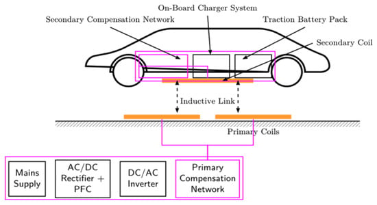
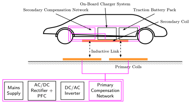
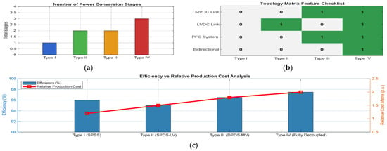
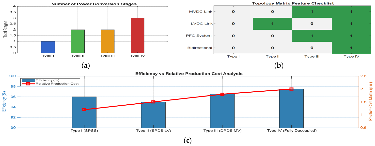
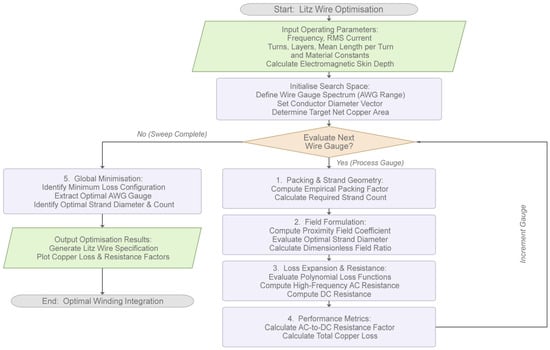
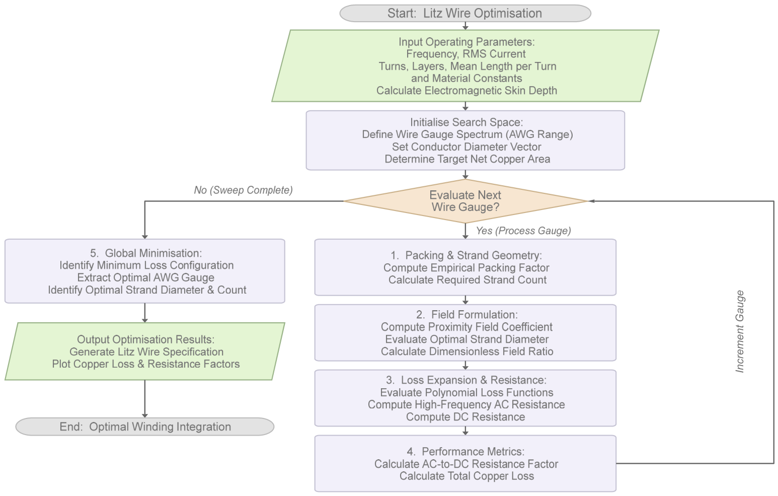
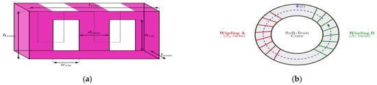
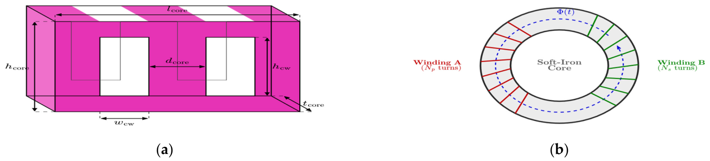
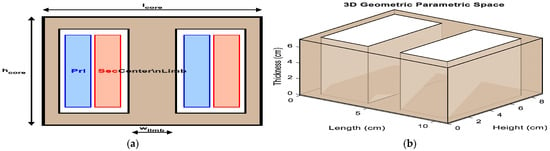
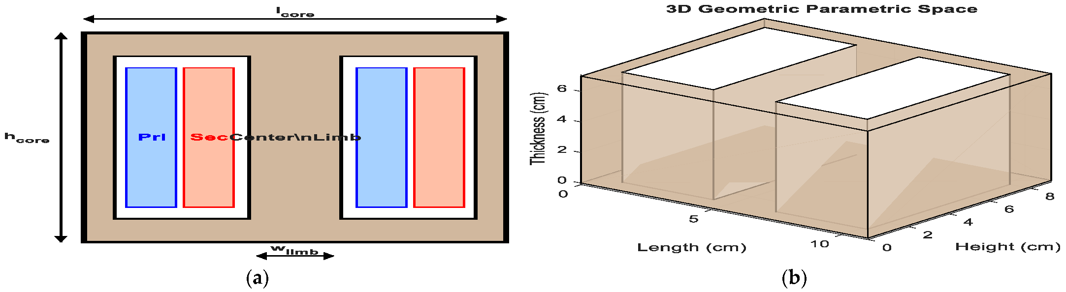
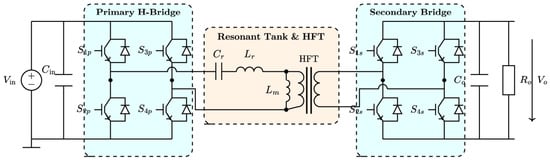
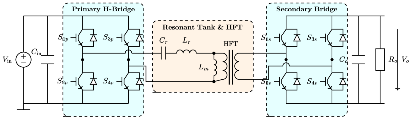
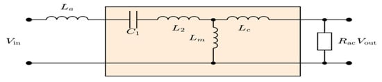
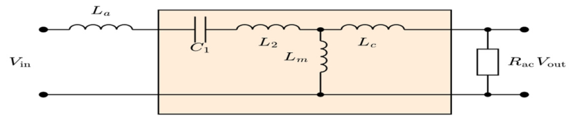
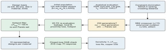
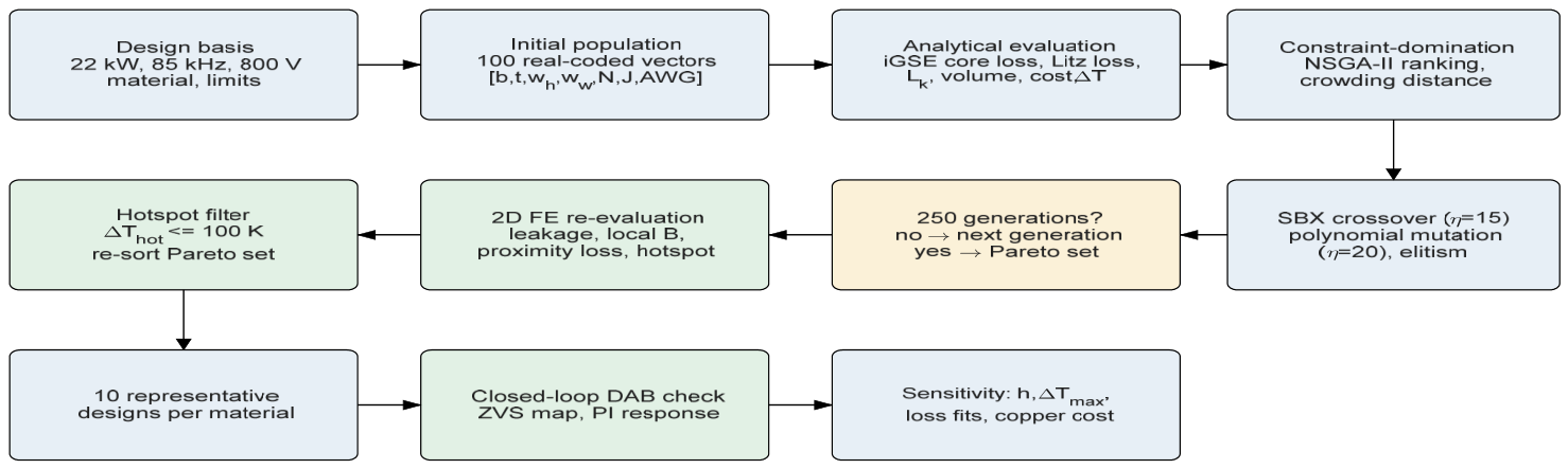
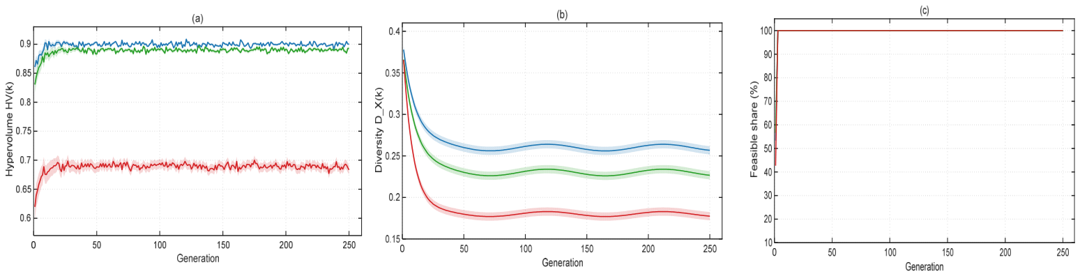
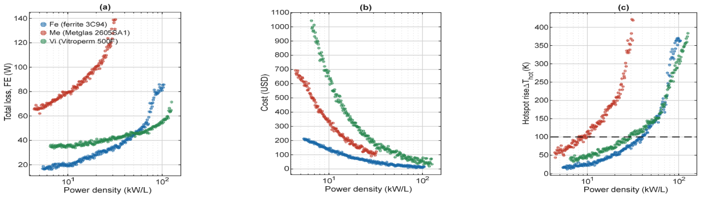
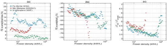
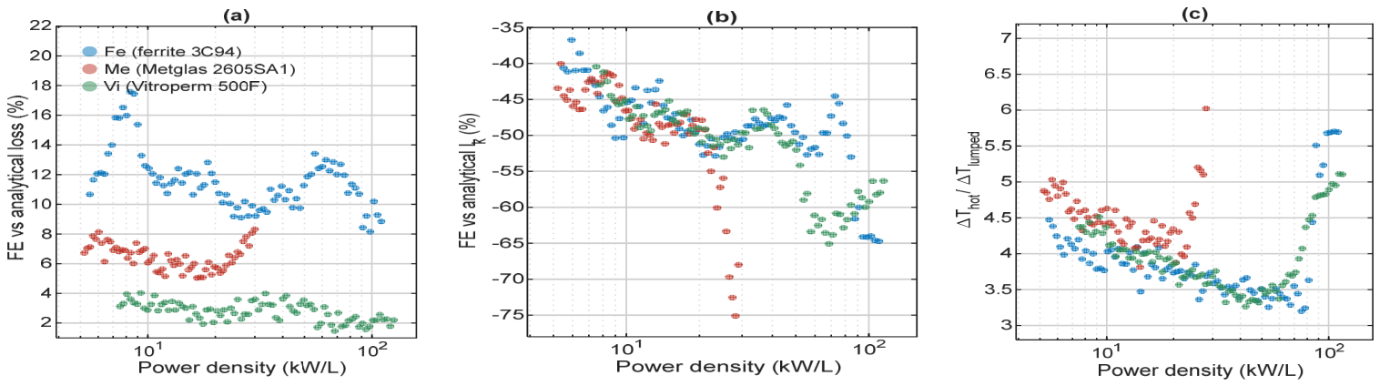
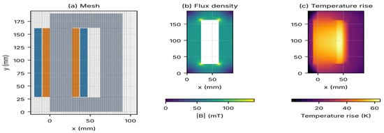
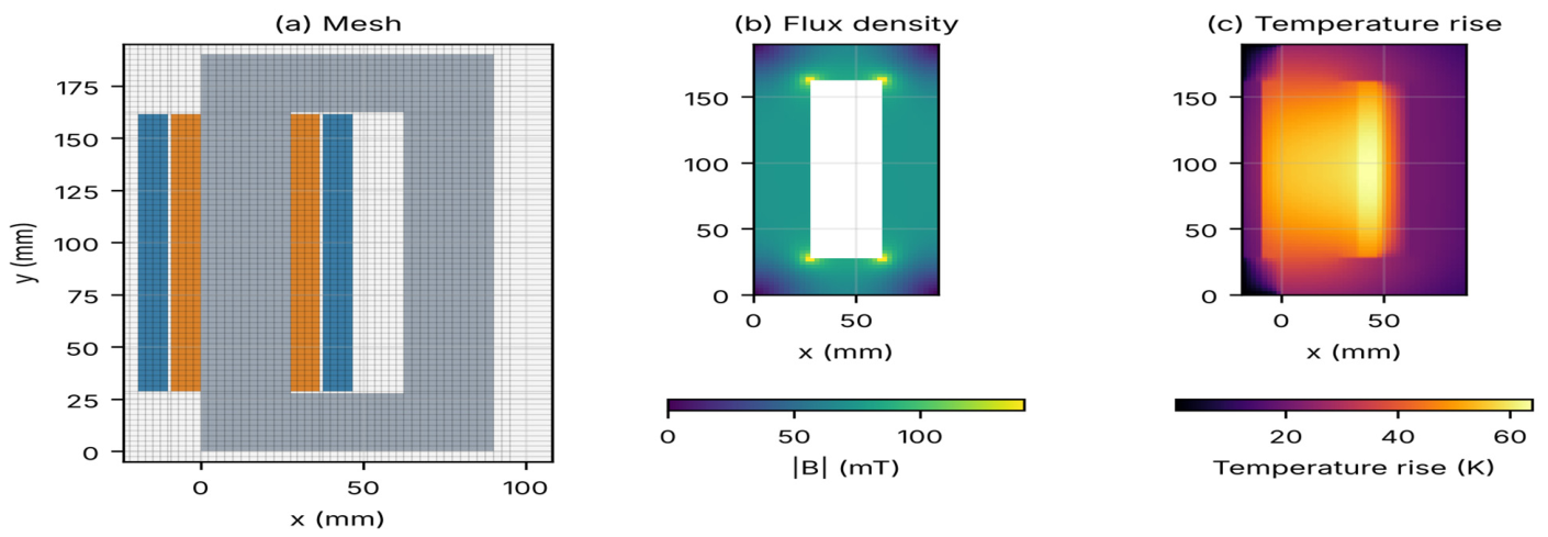
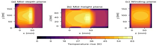
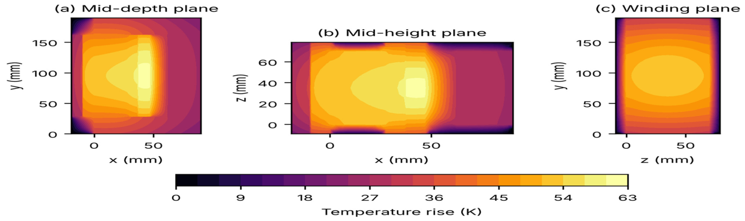
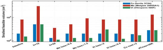
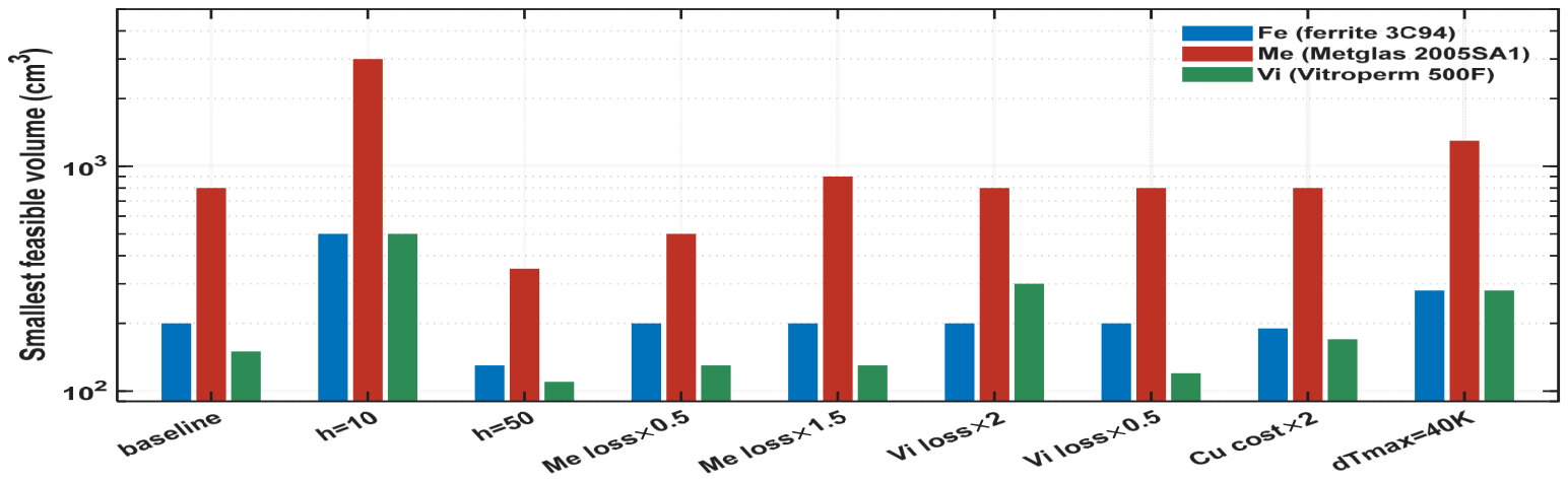
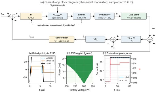
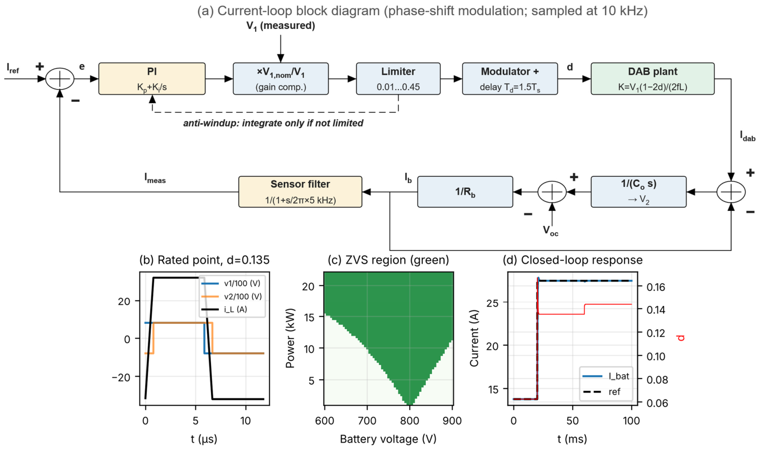
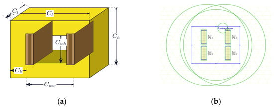
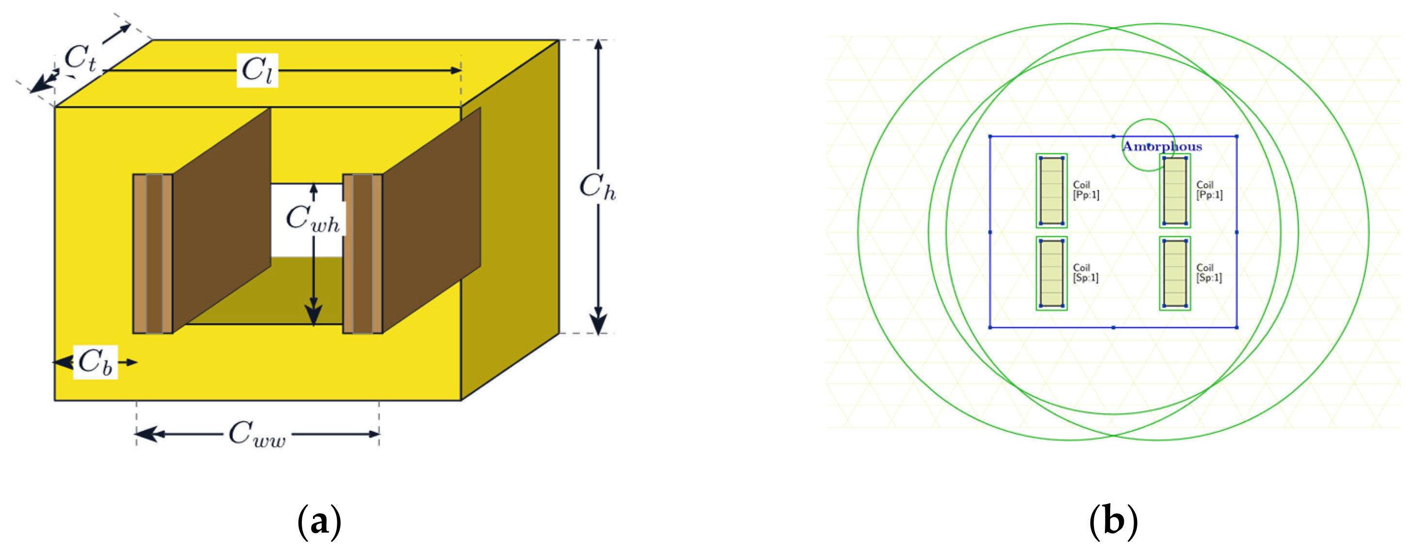
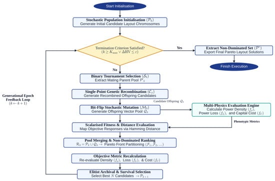
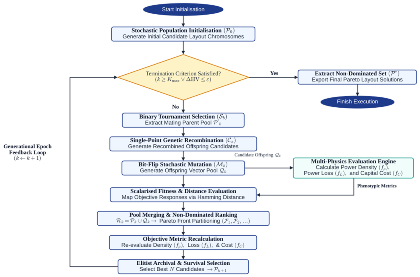
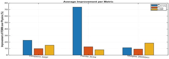
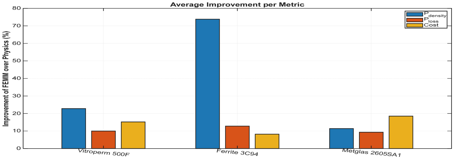
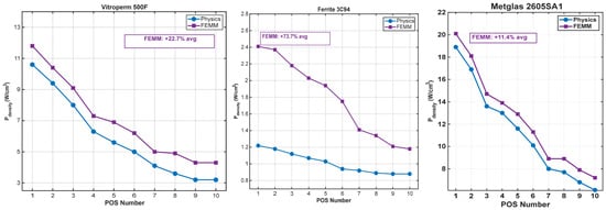
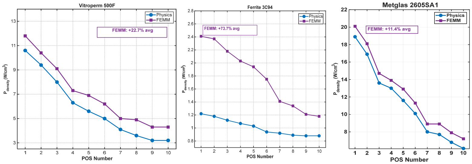
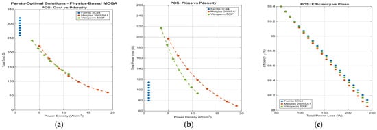
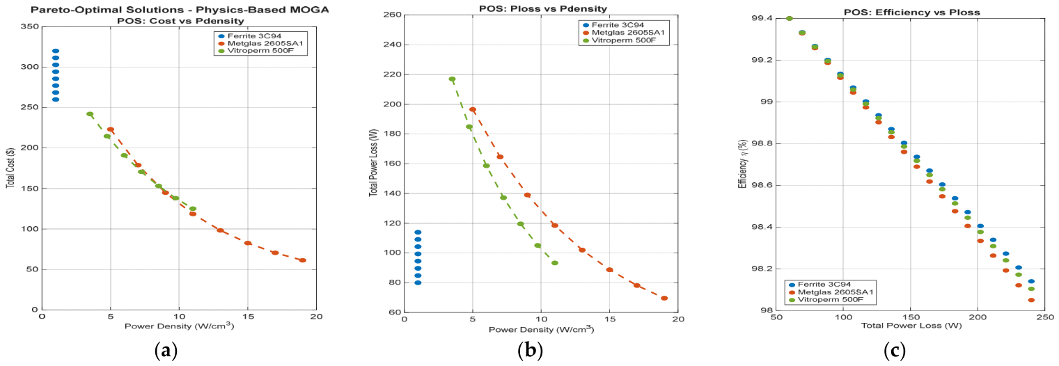
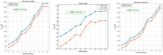
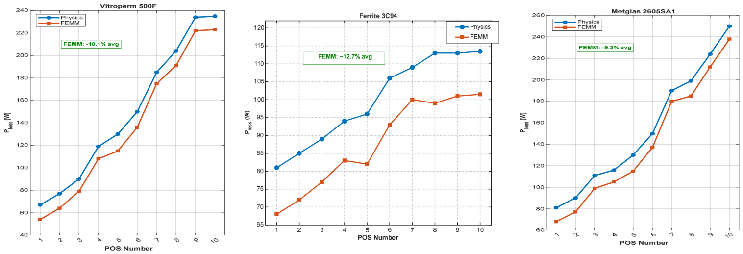
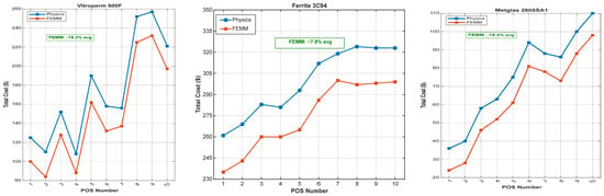
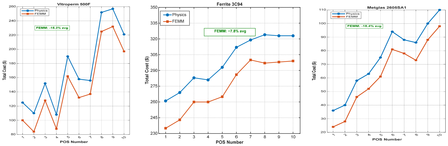
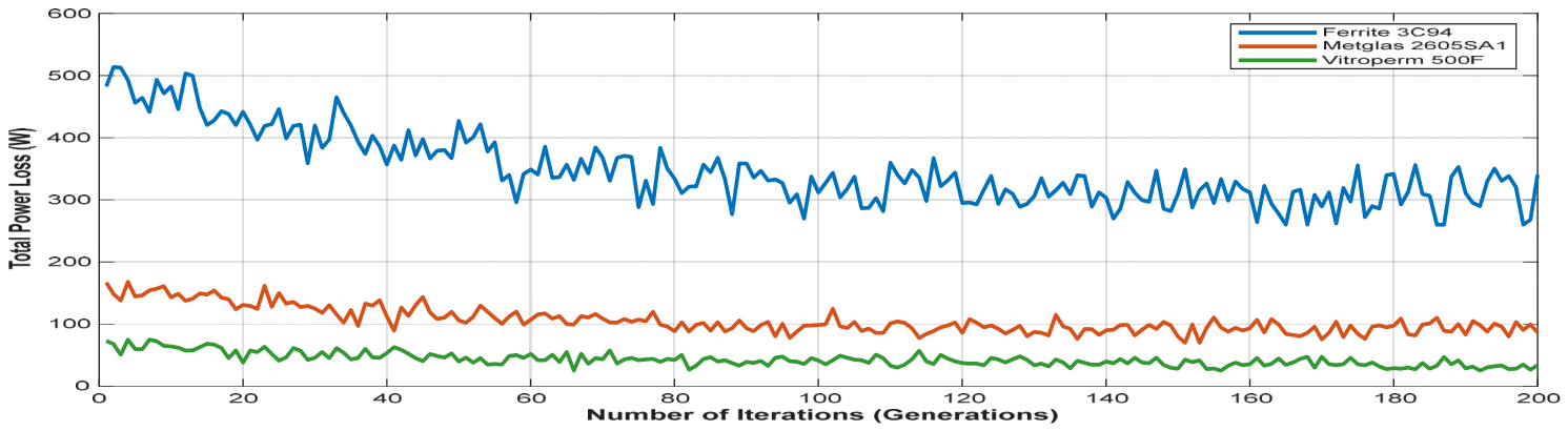
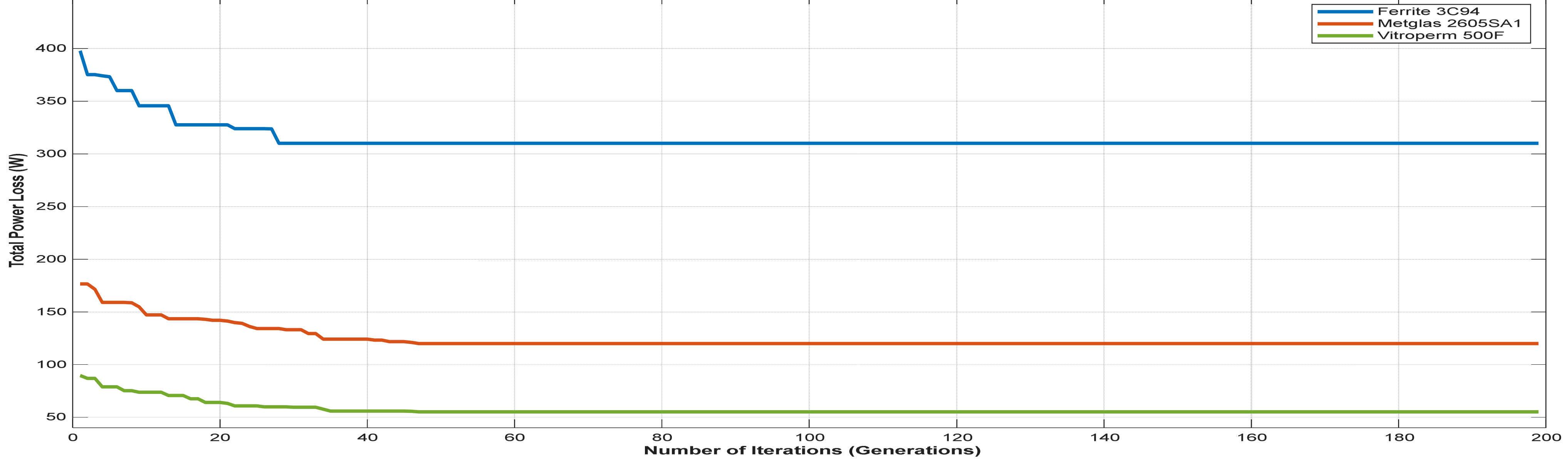
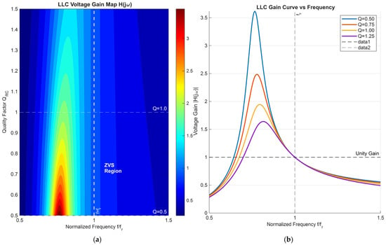
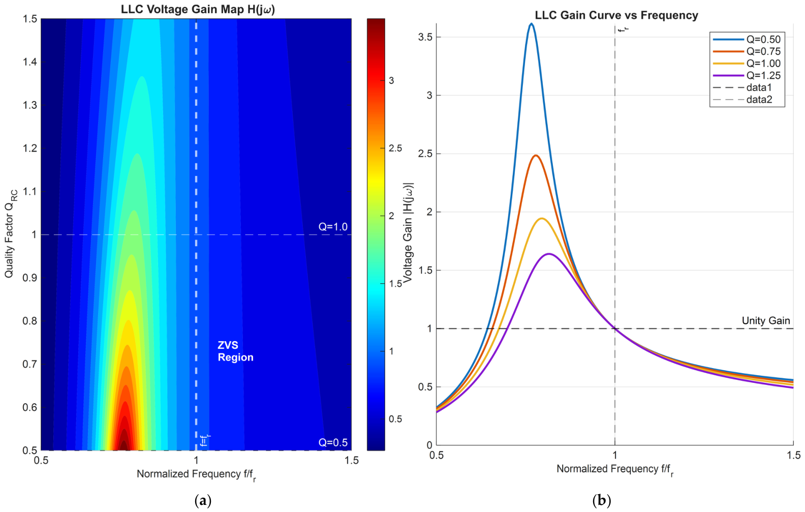
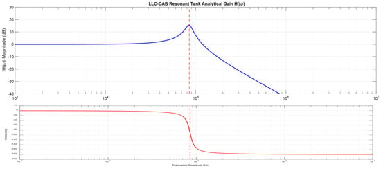
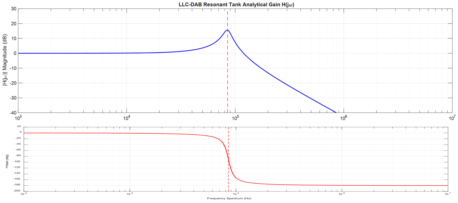
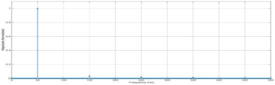
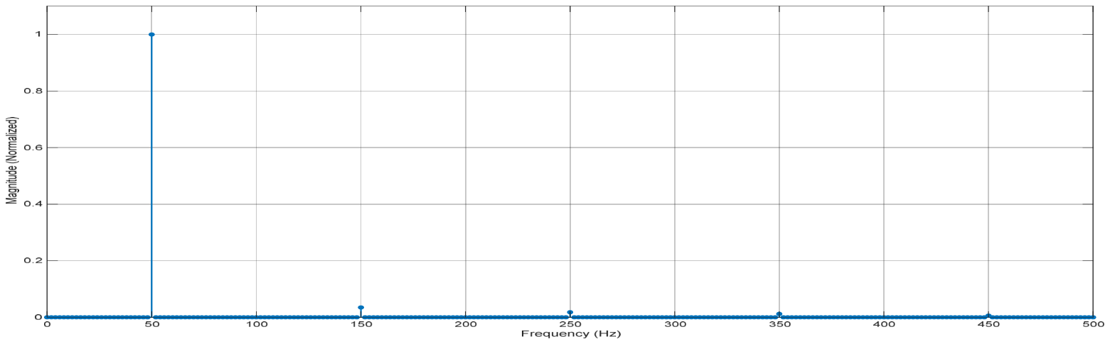
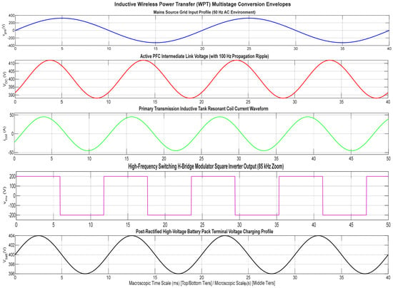
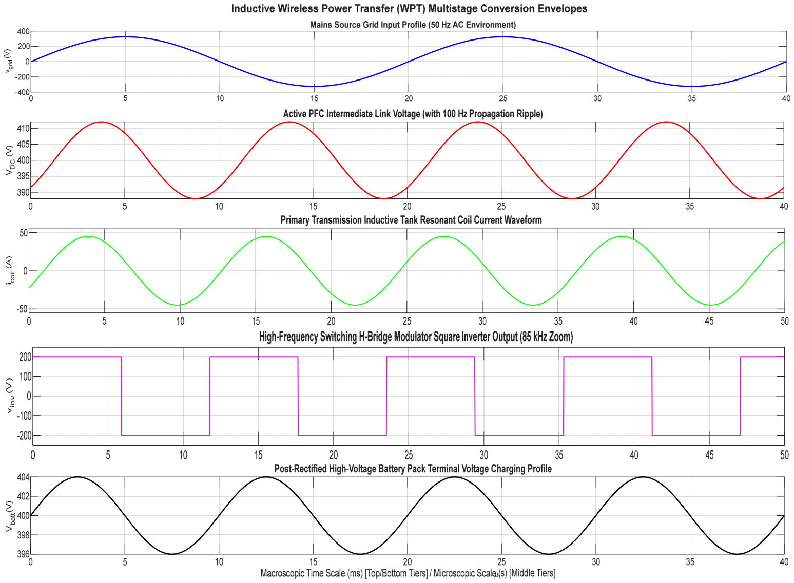
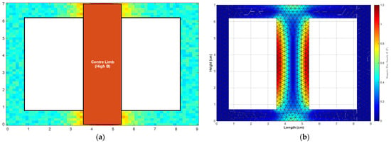
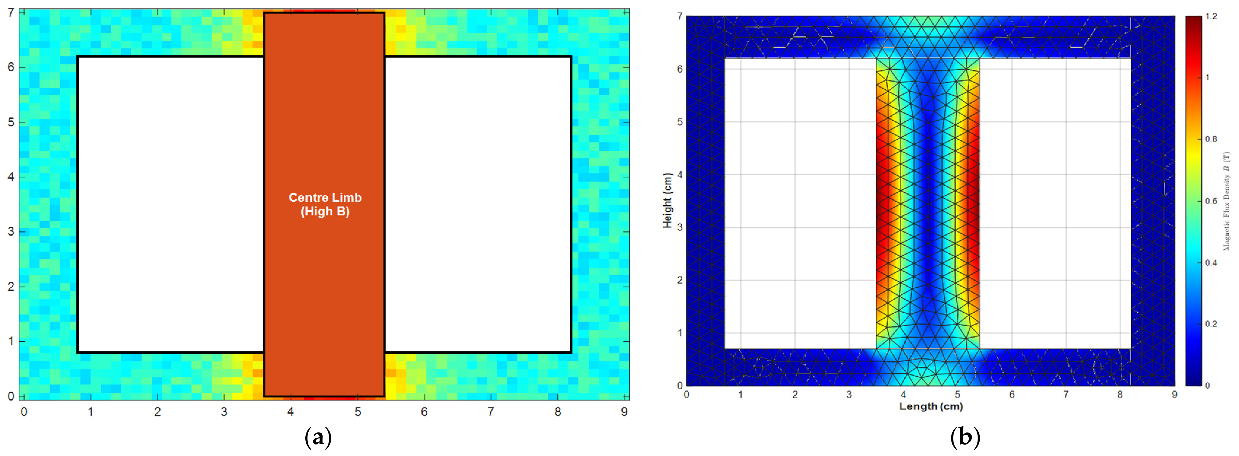
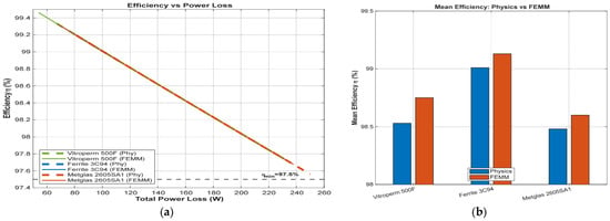
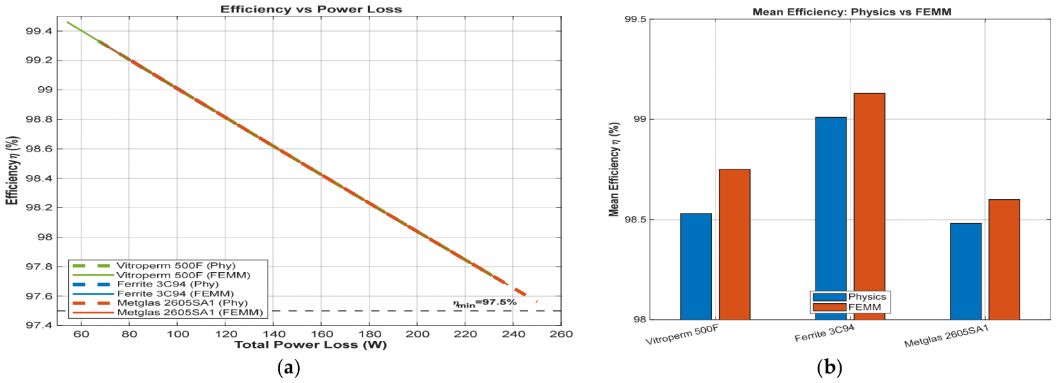
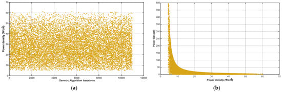
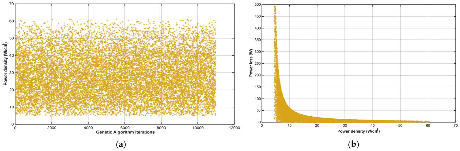
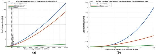
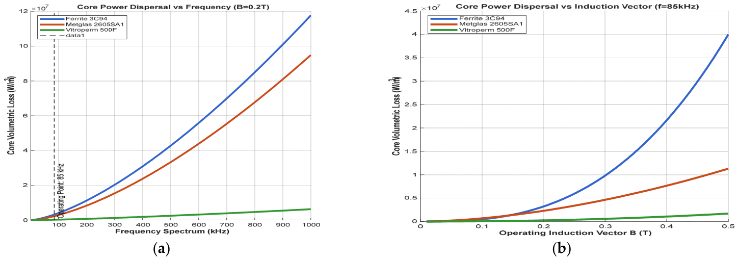
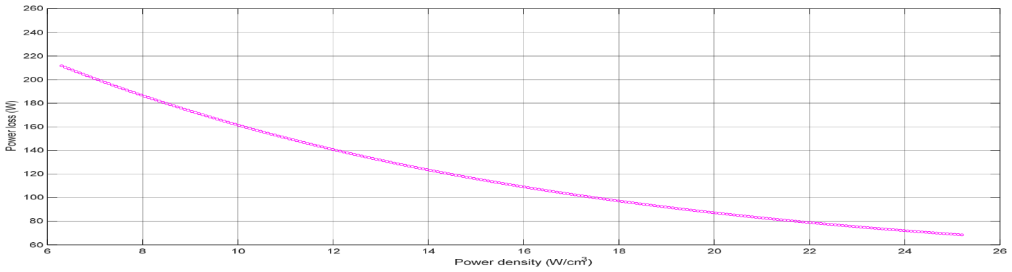
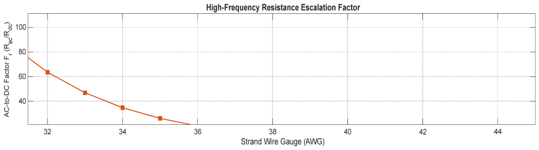
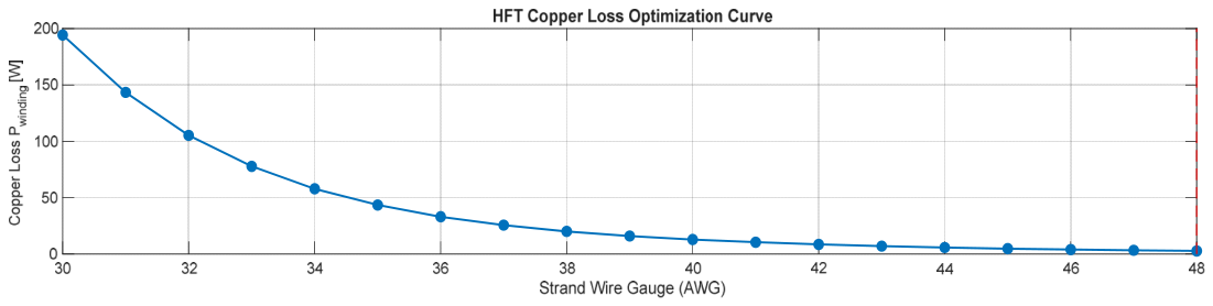


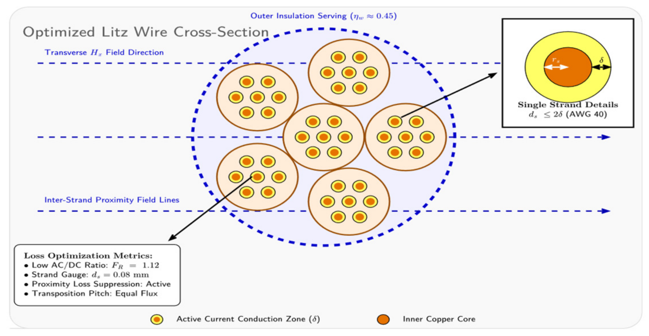
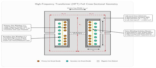
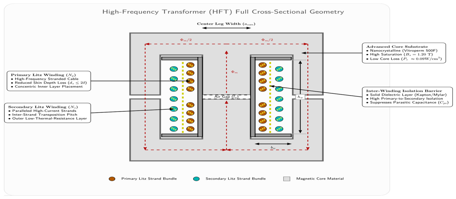
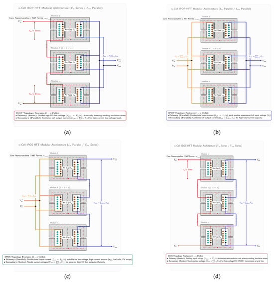
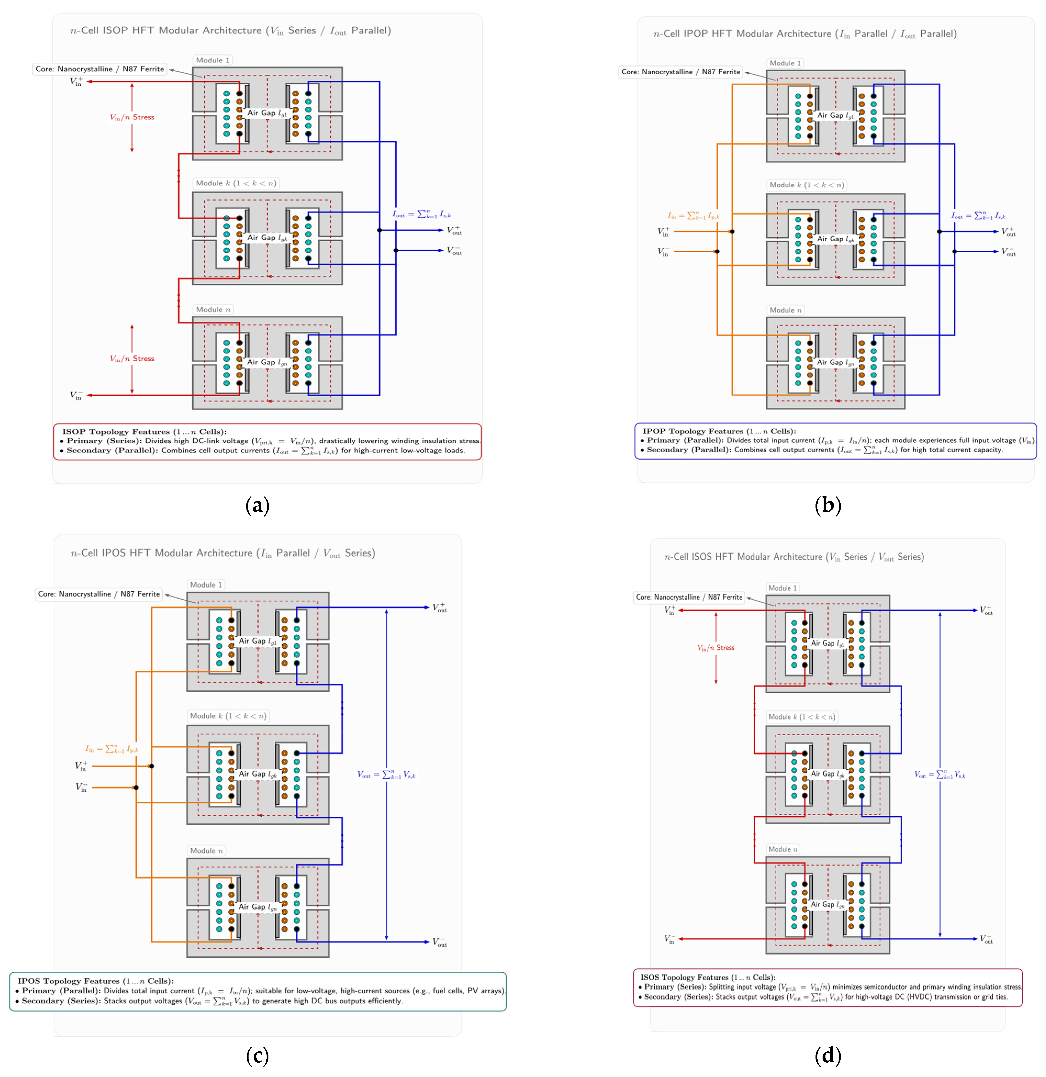

Disclaimer/Publisher’s Note: The statements, opinions and data contained in all publications are solely those of the individual author(s) and contributor(s) and not of MDPI and/or the editor(s). MDPI and/or the editor(s) disclaim responsibility for any injury to people or property resulting from any ideas, methods, instructions or products referred to in the content. |
© 2026 by the authors. Published by MDPI on behalf of the World Electric Vehicle Association. Licensee MDPI, Basel, Switzerland. This article is an open access article distributed under the terms and conditions of the Creative Commons Attribution (CC BY) license.