Autonomous Electric Vehicles as Mobile Data Centers: Energy, Emissions, and Mitigation Across Deployment Eras and Grid Scenarios

Highlights

What are the main findings?

• Grid carbon intensity is the decisive emission lever: for a 500-million-vehicle fleet, compute-only CO₂ falls from ~337 Mt CO₂e/yr (coal) to ~4.5 Mt CO₂e/yr (wind)—a reduction of ~98.7% for the compute component alone. Including propulsion, combined fleet CO₂ falls from ~1567 Mt/yr to ~21 Mt/yr on the same grid transition.
• A 500-million-vehicle Level 4 autonomous fleet operating 3 h/day generates 411 TWh/yr of compute energy—matching the entire 2024 global data centerelectricity consumption (≈415 TWh).

What are the implications of the main findings?

• Advancing both compute hardware efficiency and propulsion system performance are essential complementary strategies for minimizing the global environmental footprint of autonomous electric vehicles.
• AV compute energy deserves a separate accounting category from propulsion; at scale, it rivals the entire global data center industry, making grid decarbonization the single most impactful mitigation lever.

Abstract

The rapid advancement of autonomous electric vehicles toward Level 4 full self-driving capability introduces a new and growing energy burden: onboard artificial intelligence computers and sensors require 450 to 1200 W of continuous system power during automated operation. This paper uses a 750 W reference that spans the full Level 4 system boundary—sensing, computing, networking, power conversion, and thermal management—based on the publicly available commercial hardware specifications. The autonomy load reduces electric vehicle range by 4 to 14% depending on vehicle speed, with the largest penalty in low-speed urban service where Level 4 is deployed first. For fleets of 50, 300, and 500 million vehicles operating 3 h/day (near-term ~2030, mid-term ~2035, long-term ~2040), onboard compute energy reaches 41, 246, and 411 TWh/yr, respectively. The long-term figure approximately matches the 2024 global data centerelectricity benchmark (~415 TWh). Across five grid carbon intensities, fleet CO₂ outcomes span two orders of magnitude: compute-only emissions range from ~4.5 Mt CO₂e/yr (wind) to ~337 Mt CO₂e/yr (coal) for the 500-million-vehicle case. Total fleet energy including propulsion reaches 1911 TWh/yr for 500 million vehicles—a load relevant to grid infrastructure planning, since unlike data centers, the EV fleet imposes a geographically distributed demand across the utility network. An integrated efficiency roadmap shows that advanced chip design, solid-state sensing, and adaptive power management can reduce per-vehicle compute power to approximately 218 W full system (71% reduction from 750 W) by 2035–40; advanced chip designs alone could target 100–130 W for the compute component.

1. Introduction

The transportation sector is undergoing fundamental change through the combined development of electrification, connectivity, artificial intelligence, and edge computing. Autonomous vehicles are one of the most computationally demanding results of this change. They must sense the road, interpret complex scenes, predict the motion of other road users, plan a safe path, and control the vehicle in real time. Electric propulsion makes the energy used by these functions visible as a direct battery load.

SAE International defines six levels of driving automation [1]. The complete dynamic driving task is assigned to the automated driving system at Levels 4 and 5 within the conditions of its operational design domain. Most production vehicles today provide Level 1 or Level 2 driver assistance. Level 3 permits conditional automation while requiring a human fallback. Level 4 transfers the complete driving task and fallback response to the automated system within a defined operating domain. Level 5 extends that objective to unrestricted driving conditions. Table 1 summarizes these levels with representative compute power ranges.

Table 1. SAE driving automation levels [1]. Compute power ranges shown in column 4 are author estimates based on current production hardware; they are not defined in SAE J3016.

SAE Level	Name	Description	Compute Power (Typical, W)	Example
0	No Automation	Driver performs all driving tasks	~10–50	Base Vehicle
1	Driver Assistance	ADAS assists steering or braking	~50–200	ACC Lane keeping
2	Partial Automation	ADAS controls both steering and braking	~100–300	Tesla Auto Pilot
3	Conditional	System drives; driver must be ready as fallback	~300–500	Mercedes S-Class
4	High Automation	System drives within ODD; no fallback driver needed	~500–1500	Waymo robotaxi
5	Full Automation	System drives all conditions; no driver required	>1000	Future system

Companies including Waymo, Zoox, Baidu Apollo Go, and WeRide are actively deploying Level 4 robotaxi services in geofenced urban areas. Mercedes-Benz has received regulatory approval for Level 3 conditional automation in the United States. These deployed systems require onboard compute platforms consuming 700 W to 1.5 kW per vehicle—well beyond the modest electronics budgets of earlier driver-assistance systems [2,3,4].

A Level 4 system may combine multiple cameras, radars, LiDAR units, ultrasonic sensors, satellite navigation, and inertial measurement. Their raw streams can reach tens of gigabytes per second before selection, compression, and feature extraction [5,6]. The compute stack must fuse these streams and complete perception, localization, prediction, planning, and control within strict deadlines. It must also support diagnostics, cybersecurity, data logging, and continuous safety supervision [5,7].

Commercial automotive processors now deliver hundreds or thousands of tera-operations per second (TOPS). However, TOPS is a peak arithmetic rate, not an energy measure. Published values may describe a chip, a board, a developer platform, or a complete vehicle computer [2,8,9,10,11]. They may omit sensors, memory, low-voltage conversion, networking, and cooling. A fleet analysis therefore needs a stated system boundary and measured average power rather than a single vendor specification.

The International Energy Agency estimated that data centers used about 415 TWh in 2024 and projected about 945 TWh in 2030 in its base case [12]. Sudhakar, Sze, and Karaman showed that computing across a widely deployed autonomous fleet could produce emissions comparable with those of the data center sector under plausible combinations of fleet size, computer power, driving time, and grid carbon intensity [13]. That study also showed why a single deterministic forecast is insufficient. Earlier broad analyses of automated vehicle energy and emissions—including those of Wadud, MacKenzie, and Leiby [14], and Taiebat et al. [15]—had identified onboard computing as a distinct and growing contributor to fleet-level energy demand.

Broader environmental reviews reach a similar conclusion from a different direction. Automation may reduce energy through smoother control, coordination, and vehicle sharing. Yet, induced travel, empty repositioning, larger service demand, and digital infrastructure can offset those gains [15]. Life-cycle outcomes depend on electricity supply, vehicle occupancy, service life, battery production, and changes in travel demand [14,16,17,18,19,20]. Hence, all these aspects must be considered when estimating the overall energy consumption of an autonomous vehicle.

This paper establishes 750 W as a standardized Level 4 compute reference, quantifies fleet-scale energy across three deployment eras (near-term~2030, mid-term~2035, long-term~2040), analyzes CO₂ across five grid carbon intensities, benchmarks results against time-matched global data centerprojections, and evaluates technical mitigation strategies. The 750 W reference is reasonable, based on the advanced technologies and the future strategies of various system manufacturers. Relative to the foundational study by Sudhakar, Sze, and Karaman [13], this paper makes six distinct contributions: (a) System boundary: Sudhakar et al. explicitly excluded sensor power, modeling only DNN inference hardware. This paper defines a full system boundary—sensing (30–190 W), computing, memory, networking, power conversion losses, and incremental cooling—based on public commercial hardware specifications. (b) Duty cycle: Sudhakar et al. used Q ~0.79 h/day (the 2017 U.S. national average driving time). This paper uses 3 h/day for a Level 4 personal AV and adds 8 h/day and 10 h/day commercial scenarios. (c) Data centerbaseline: updated from the 2018 benchmark (~140 Mt CO₂, 205 TWh) to the 2024 IEA figures (~180 Mt CO₂, 415 TWh) and the 2030 projection (~945 TWh). (d) Commercial comparison: power cases are grounded in publicly disclosed hardware profiles from deployed Level 3/4 systems. (e) Range-penalty analysis: the vehicle-level energy impact as a function of vehicle speed is quantified (Section 4). (f) Efficiency roadmap: a positive mitigation roadmapis provided, showing achievable per-vehicle power reductions with measurable milestones. A note on propulsion energy: this paper reports both compute-only and combined (compute + propulsion) fleet energy. The combined figure is relevant for power-grid planning because, unlike data centers—which can be co-located with dedicated generation capacity—the AEV fleet imposes a geographically distributed load across the utility network, including residential feeders and substations. At 500 million vehicles, this distributed demand warrants separate attention from grid operators and infrastructure planners, independently of the data centercomparison.

Section 2 describes the sensing, computing, V2X, and thermal architecture, together with current commercial deployments. Section 3 defines the power cases and governing equations. Section 4, Section 5 and Section 6 examine vehicle energy, fleet electricity, and carbon emissions. Section 7 develops the mobile data centeranalogy and evaluates efficiency strategies. Section 8 and Section 9 address broader system effects, research needs, and the long-term outlook. Section 10 summarizes the findings.

2. AV System Architecture and Sensor Data

A Level 4 automated driving system integrates sensing, computing, communications, and thermal management into a cohesive onboard architecture. This section describes the functional pipeline, the sensor data generated, and the commercial platforms that define the realistic power envelope. The energy boundary used throughout this analysis is also defined here.

2.1. Onboard Autonomy Architecture

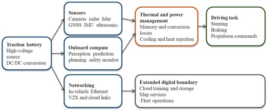
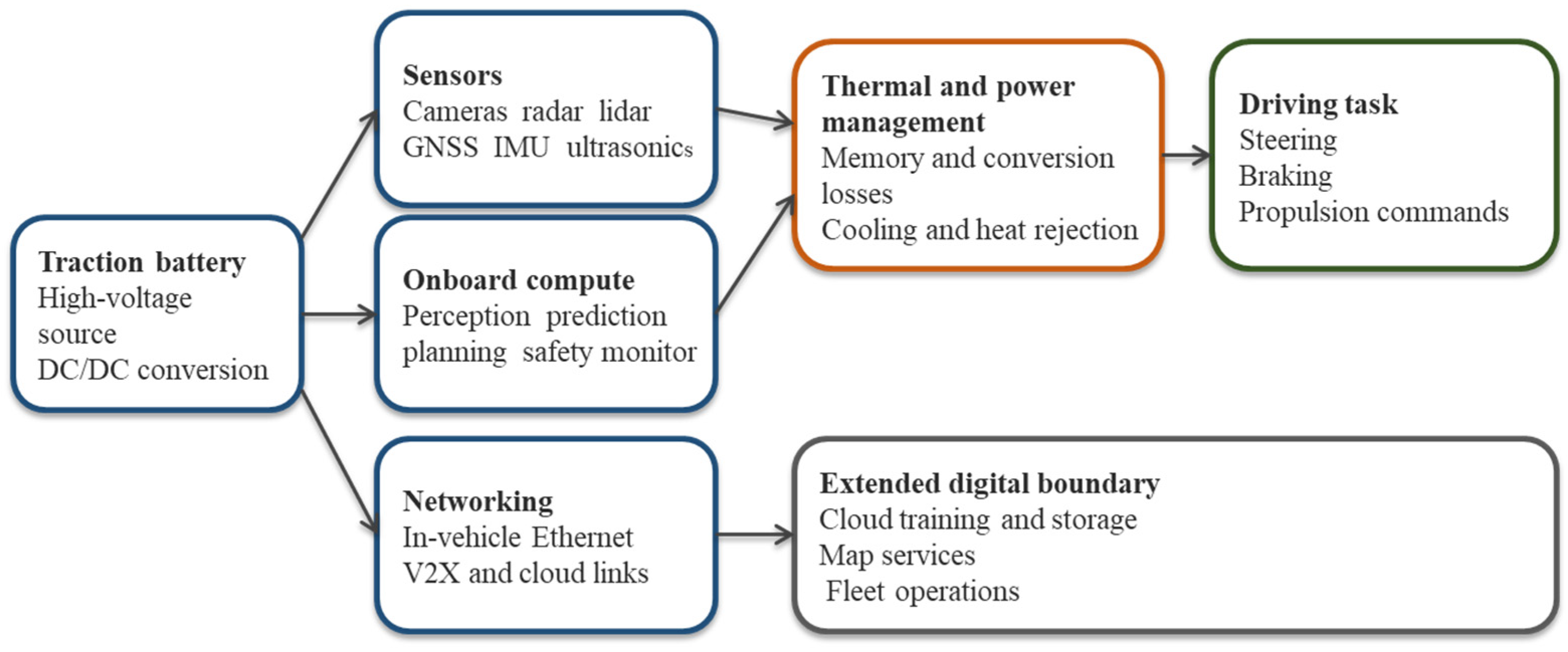
An automated driving system converts heterogeneous sensor streams into vehicle motion commands. A typical pipeline performs sensor synchronization, localization, object detection, tracking, scene prediction, trajectory planning, control, and continuous safety monitoring [5,7]. Figure 1 shows the AV functional pipeline and the energy and data boundary used in this study.

Figure 1. Energy and data boundary used in this study.

The core boundary includes sensors, onboard computing, memory, in-vehicle networking, low-voltage conversion losses, and the incremental thermal load required to reject their heat. Traction, cabin climate control unrelated to the autonomy stack, charging losses, manufacturing, road infrastructure, cloud training, and fleet management services are excluded because the focus of this paper is on energy consumption due to onboard computing and sensors.

2.2. Sensor Suite, V2X Communication, and Data Rates

Modern Level 4 platforms deploy multiple sensing modalities for redundancy and complementarity. LiDAR systems generate 3D point clouds at 10–20 Hz; a single 128-beam unit produces roughly 2.4 million points per second. Cameras (8–30 channels at 8 MP and 30 fps) contribute high-bandwidth video. Radar provides all-weather velocity and range. Ultrasonic sensors cover close distances. GPS and IMU estimate vehicle position and motion. Table 2 summarizes typical data rates and power for each modality [3,5,6].

Table 2. Illustrative sensor interface data rates and power ranges in a 2025-era Level 4 autonomous vehicle. Power ranges are from [3] and specs from manufacturers.

Sensor	Units (Typical L4)	Interface Data Rate (GB/s)	Assumed Suite Power (W)
Camera (HD, multi-channel)	8–30 channels, 8 MP/30 fps	2.88–10.80 Gbyte/s	20–60
LiDAR (solid-state/spinning)	2–6 units, 10–20 Hz	0.077–0.230 Gbyte/s	3–100
Radar (imaging 4D)	6–9 units	0.3–0.5 Gbyte/s	5–20
Ultrasonic	12 units	<0.1 Gbyte/s	1–3
GPS/IMU	1 unit	<0.01 Gbyte/s	3–5
Total raw (uncompressed)	—	Not determined	30–190

Sensor hardware interface throughput depends on resolution, frame rate, encoding, and configuration; no all-sensor aggregate rate is claimed here. The camera and LiDAR entries in Table 2 use the illustrative interface configurations below; generated data are distinct from retained or uploaded data. Table 2 gives the per-sensor basis: at 8 MP, 30 fps, and 12 bits/pixel, a single camera outputs approximately 0.36 Gbyte/s; 8–30 cameras therefore contribute 2.9–10.8 Gbyte/s. At 2.4 million points/s and 16 bytes/point, 2–6 LiDAR units contribute 0.077–0.230 Gbyte/s. At 3 h/day and 365 days/year, the stated camera and LiDAR interfaces generate approximately 11.4–42.6 and 0.30–0.91 PB/year, respectively, before retention or compression. The vast majority is processed locally in real time. An illustrative cloud-upload volume (0.5–5 Tbyte per vehicle per year) is used for AI model training, fleet learning, edge-case analysis, and software improvement.

Connected and automated vehicles communicate via vehicle-to-everything (V2X) technology. Vehicle-to-vehicle (V2V) links share speed, location, and heading data for cooperative collision avoidance. Vehicle-to-infrastructure (V2I) connections interact with traffic signals and road sensors. Vehicle-to-cloud (V2C) transmission enables fleet learning and AI model updates. V2X adds modest continuous power at the vehicle level; its primary energy significance lies in the cloud and network infrastructure it connects to, which is tracked separately and is outside the core boundary of this study [7,21]. Cooperative adaptive cruise control enabled by V2V can reduce aerodynamic drag in platoon formation by 15–25% [14], partially offsetting the compute energy penalty.

2.3. Compute Platforms and Power Boundaries

Published platform specifications cannot be placed in a single ranking without qualification. A board-level developer kit can include memory and interfaces but exclude vehicle sensors and cooling. A chip value may exclude external memory and power conversion. A reference architecture may include two computers for redundancy without publishing a normalized system total [2,8,9,10,11]. Table 3 lists major platforms with stated power boundaries.

Table 3. Current and next-generation AV compute platforms with system power boundaries. TOPS ratings use inconsistent workloads and precisions; direct comparison requires common test conditions [2,8,9,10,11].

Platform	TOPS	System Power (W)	Notes
Tesla HW5 (single)	~2000	~800	Camera-dominant; chip power reported †
Tesla HW5 (dual, fail-operational)	~4000	~1600	Estimated; not confirmed by Tesla †
NVIDIA DRIVE Thor (single SoC)	~1000 INT8	350 (dev kit)	[8]; 350 W development-system rating, not chip TDP
NVIDIA Hyperion (2 × Thor + sensors)	4000+	650–1100	Full L4 reference architecture
Mobileye EyeQ Ultra (chip)	176	~100	Very low chip power; multi-chip system for L4
Qualcomm Snapdragon Ride (L4/L5)	700+	~130 (chip)	Single SoC; sensors excluded

† Tesla HW5 (also referred to as AI5) TOPS estimate is based on industry reports citing TSMC and Samsung foundry orders; the 2000–2500 TOPS range has not been officially confirmed by Tesla. Source: Notebookcheck, “Tesla HW5 FSD computer specs leak out as production is entrusted to TSMC and Samsung,” 2024. Available: https://www.notebookcheck.net/Tesla-HW5-FSD-computer-specs-leak-out-as-production-is-entrusted-to-TSMC-and-Samsung.1038965.0.html (accessed on 5 October 2026). Power estimate (~800 W single, ~1600 W dual) is extrapolated from HW4 disclosures and is similarly unconfirmed.

Across these platforms, 0.75 kW is adopted as the reference system-level power for a redundant Level 4 installation with sensors, networking, conversion losses, and incremental cooling. This value is consistent with reported hardware, measured deployments, and prior literature [3,4,13].

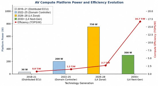
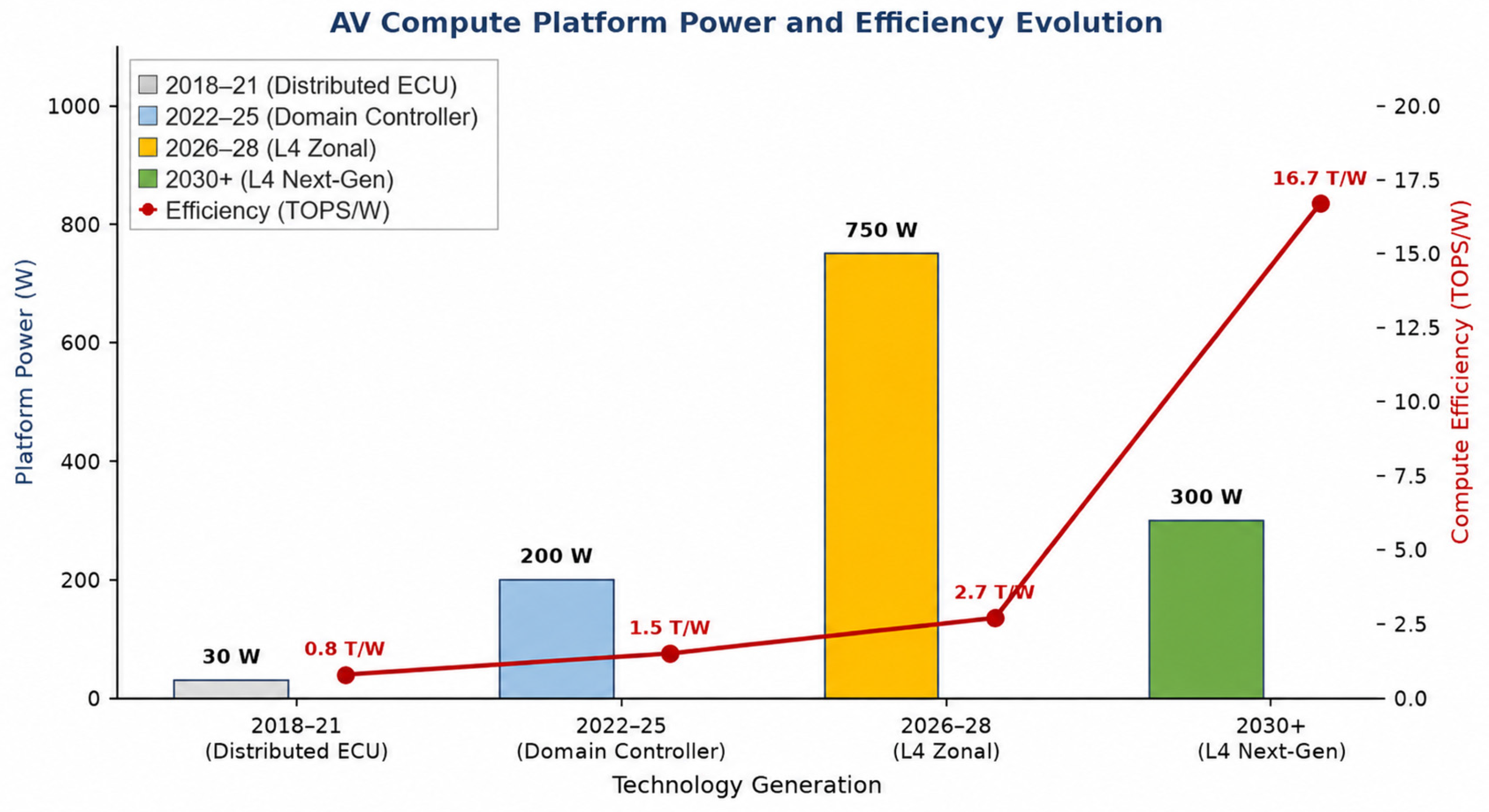
Automotive compute efficiency has improved across generations. NVIDIA’s progression from Xavier (~1 TOPS/W in 2018) to Orin (~5 TOPS/W in 2022) and subsequently to Thor (projected >10 TOPS/W) illustrates roughly a 2× improvement per generation [8,9]. Despite this, absolute system power has not fallen because the Level 4 compute task is approximately 10× larger than Level 3. Figure 2 shows this efficiency trajectory alongside absolute power.

Figure 2. Average AV compute platform power (W) and efficiency (TOPS/W) evolution, 2018–2030+. Efficiency improves per generation, yet absolute system power remains in the hundreds-of-watts range due to growing task complexity.

2.4. Related Energy and Emission Studies

Recent studies have widened the analysis beyond the central computer. Van Oosterhout, Striekwold, and Wang modeled sensing, onboard processing, storage, wireless communication, and data center activity [21]. They found strong sensitivity to communication energy intensity and transmitted data volume. Rajashekara and Koppera reviewed energy and data effects of intelligent transportation across sensing, computation, communications, and traffic operations [3]. Rajashekara separately emphasized the range and emission implications of the electrical loads added by automated driving [4].

Life-cycle studies of autonomous taxi fleets show that electrification, grid decarbonization, sharing, empty travel, vehicle lifetime, and computer efficiency interact over time [16]. Laarabi et al. extended the Sudhakar et al. analysis to include cloud AV infrastructure and found the combined footprint substantially larger [22]. This paper extends those analyses with three power cases, a clearer system boundary, and commercial deployment evidence.

3. AV Compute Power and Energy Model

Estimating fleet energy requires explicit power assumptions at the vehicle level. This section introduces three power cases that bracket the performance of current and near-term Level 4 hardware, and derives the equations linking per-vehicle power and duty cycle to fleet-scale electricity demand.

3.1. Reference Power Cases

Because complete Level 4 system power is rarely disclosed on a consistent basis, the analysis uses three explicit cases. Table 4 defines the cases and their empirical anchors.

Table 4. System-level autonomy power cases. The reference case is used in all headline comparisons.

Case	System Power	Empirical Anchor
Efficiency (low)	0.45 kW	446.7 W measured auxiliary load, Brown et al. [23]
Reference	0.75 kW	Redundant L4 installation with sensors, networking, and cooling (established as Reference in this paper by the author)
High-power	1.20 kW	Upper limit from Sudhakar et al.’s scenario analysis [13]

The cases are analytical boundaries, not forecasts for any named vehicle. Sensitivity to the other cases is shown where it changes the conclusion. Compute dominates the added energy budget: computing accounts for approximately 77% of the illustrative 750 W allocation specified in Section 3.2. Sensor overhead is higher in LiDAR-rich platforms and lower in camera-dominant designs.

3.2. Power Components and Operating States

System power, depending on the architecture, can be divided into sensing, central computing, memory, in-vehicle communication, power conversion, and incremental thermal management. A camera-dominant design shifts work toward image processing. A LiDAR-rich design adds optical sensing and point-cloud processing. Centralized computers may remove duplicated electronic control units and reduce wiring, but they concentrate heat and require carefully designed fallback paths. For the illustrative 750 W reference, the assumed allocation is 575 W computing, 100 W sensing, and 75 W for memory, networking, conversion, and incremental cooling; this is an analytical allocation, not a measured commercial-system breakdown. The 575 W computing allocation represents a multi-chip near-term Level 4 platform (AI SoC or module, dedicated GPU, automotive CPU, and memory/networking silicon); the 350 W NVIDIA Thor figure in Table 3 is a single next-generation SoC entry on the efficiency roadmap (Section 8.1)—these are different architecture generations.

Energy studies should distinguish active driving, ready-but-stationary operation, startup, sleep, and charging. A robotaxi may remain ready while waiting for a passenger. A private vehicle may shut down most autonomy functions when parked. These differences can produce a larger annual energy change than a modest improvement in processor efficiency. Duty cycle is therefore modeled explicitly rather than inferred from fleet size, and the hours of daily use are a very important factor.

3.3. Vehicle and Fleet Equations

For a vehicle traveling at average speed v while the autonomy stack draws constant power P, the incremental battery energy per unit distance equals P divided by v. With baseline traction energy e₀, the first-order range reduction is the ratio of autonomy energy per mile to total battery energy per mile.

Annual per-vehicle compute energy:

E_tompxt^e = P × H × 365 [kWh/yr]

(1)

For the reference case (P = 0.75 kW, H = 3 h/day): E_tompxt^e = 0.75 × 3 × 365 = 821 kWh/yr.

Annual fleet compute energy:

E_mleet = N × P × H × 365/10⁹ [TWh/yr]

(2)

where N is the fleet size and P is the system power in kilowatts. Operational carbon emissions are fleet electricity multiplied by grid carbon intensity. The model reports a range of intensities and uses the 2024 global power-sector average of 445 g CO₂/kWh as a current reference [24].

3.4. Scenario Assumptions

Table 5 summarizes the main scenario variables.

Table 5. Main scenario variables and reference values.

Variable	Value/Range	Notes
Fleet sizes modeled	50 M, 300 M, 500 M vehicles	Illustrative ~2030, ~2035, and ~2040 cases; not adoption forecasts
System power (reference)	0.75 kW	Sensitivity cases: 0.45 kW and 1.20 kW
Operating hours (reference)	3 h/day	Private AV; commercial cases: 8 h/day and 10 h/day
Annual propulsion energy	3000 kWh/yr	10,000 mi/yr × 300 Wh/mi; illustrative baseline
Grid carbon intensity	11–820 g CO2e/kWh (life-cycle)	Wind to coal (IPCC AR5); 445 g CO2/kWh operational comparison reported separately
Reference year for data centers	2024 (415 TWh) and 2030 (945 TWh)	IEA base case [12]

The current analysis is intentionally deterministic and transparent: three explicit power cases (0.45, 0.75, and 1.20 kW), three fleet sizes (50 M, 300 M, and 500 M vehicles), and five grid carbon intensities. A probabilistic approach—such as the Monte Carlo analysis used by Sudhakar et al. [13] with one million samples—would provide uncertainty bounds around the central fleet energy and emission estimates, but requires well-characterized probability distributions for fleet size, adoption schedule, and duty cycle that remain highly uncertain for a technology still in early deployment. Probabilistic scenario analysis, including regional adoption modeling (North America, Europe, China, and the rest of the world) and technology learning rates, is recommended as a priority for future work. The extreme endpoints of this deterministic scenario space are 0.45 kW × 50 million vehicles × 1 h/day × 365 days/year/10⁹ = 8.21 TWh/year (minimum) and 1.20 kW × 500 million vehicles × 10 h/day × 365 days/year/10⁹ = 2190 TWh/year (maximum). The corresponding CO₂e bounds span 0.090 Mt/year (wind grid at 11 g/kWh) to 1795.8 Mt/year (coal grid at 820 g/kWh); these are assumption bounds, not confidence intervals.

4. Vehicle-Level Energy Analysis

At the vehicle level, onboard autonomy adds a persistent electrical load that reduces battery range and raises annual energy consumption. This section quantifies that addition for representative duty cycles, explains how vehicle speed shapes the range penalty, and compares the model with chassis dynamometer measurements.

4.1. Propulsion and Annual Autonomy Energy

A representative mid-size electric vehicle uses about 300 Wh per mile in mixed driving [25,26]. At 10,000 miles per year, annual propulsion energy is approximately 3000 kWh/yr. This value is an illustrative baseline. Vehicle mass, aerodynamics, speed, temperature, grade, and traffic can change it substantially.

Autonomy energy depends on power and active hours rather than distance alone. Table 6 shows annual electricity for several duty cycles at the three power levels. The compute share is the ratio of autonomy energy to total vehicle energy (propulsion plus autonomy).

Table 6. Annual onboard autonomy energy by vehicle use case.

Use Case	H (h/day)	P = 0.45 kW (kWh/yr)	P = 0.75 kW (kWh/yr)	P = 1.20 kW (kWh/yr)	Compute Share 1 (%)
Private car (occasional)	1	164	274	438	8.4
Personal AV (reference)	3	493	821	1314	21.5
Commercial fleet	8	1314	2190	3504	14.3
Full-service robotaxi	10	1643	2738	4380	14.3

Note: ¹ Compute share uses 0.75 kW reference and 3000 kWh/yr propulsion for personal vehicles; commercial propulsion uses 15 mph at the stated operating hours and 300 Wh/mile.

At the reference level (0.75 kW, 3 h/day), the autonomy system adds 821 kWh/yr to a propulsion baseline of 3000 kWh/yr. Total per-vehicle energy is 3821 kWh/yr. Compute represents approximately 21.5% of the total, compared with less than 5% for current Level 2 vehicles operating at roughly 100 W for 1 h/day.

The same 0.75 kW system uses only 274 kWh/yr at one hour per day but 2738 kWh/yr at ten hours per day. Commercial service therefore makes the digital load comparable to a large fraction of annual propulsion energy, even when the hardware is unchanged.

4.2. Why Average Speed Matters

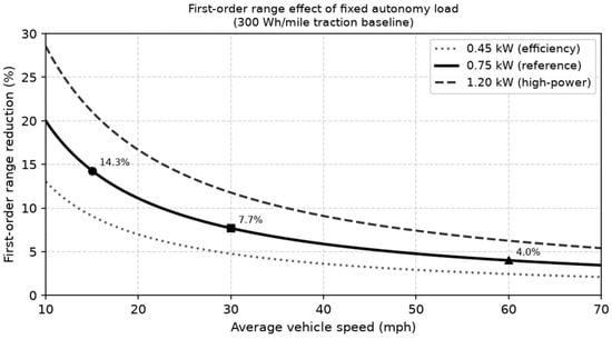
A fixed auxiliary load adds energy per unit time, whereas propulsion studies usually report energy per unit distance. The conversion depends on average speed. At 0.75 kW, the autonomy stack adds 50 Wh per mile at 15 mph, 25 Wh per mile at 30 mph, and 12.5 Wh per mile at 60 mph. Relative to a 300 Wh per mile traction baseline, the first-order range reductions are 14.3%, 7.7%, and 4.0%, respectively. A single range penalty percentage therefore hides the duty cycle that produced it. Figure 3 illustrates this speed dependence.

Figure 3. First-order range effect of a fixed autonomy load for a 300 Wh per mile traction baseline. Annotated markers show the reference (0.75 kW) values at 15, 30, and 60 mph.

Table 7 extends the speed sensitivity to all three power cases. The range reduction is largest in low-speed urban service—precisely the environments where Level 4 robotaxis and delivery vehicles operate first. Higher speeds reduce the penalty but cannot eliminate it.

Table 7. Vehicle energy sensitivity by operating speed. Traction baseline: 300 Wh/mile. Range reduction = autonomy energy/(traction + autonomy energy) × 100%.

Avg. Speed (mph)	Autonomy Energy (Wh/mi) 0.45 kW	Autonomy Energy (Wh/mi) 0.75 kW	Autonomy Energy (Wh/mi) 1.20 kW	Range Reduction (%) 0.45 kW	Range Reduction (%) 0.75 kW	Range Reduction (%) 1.20 kW
15	30.0	50.0	80.0	9.1	14.3	21.1
25	18.0	30.0	48.0	5.7	9.1	13.8
35	12.9	21.4	34.3	4.1	6.7	10.3
45	10.0	16.7	26.7	3.2	5.3	8.2
55	8.2	13.6	21.8	2.7	4.3	6.8
65	6.9	11.5	18.5	2.3	3.7	5.8

This speed dependence is most consequential for robotaxis, urban delivery vehicles, and low-speed shuttles. Those services combine long operating hours with low average speed. They are also the services most likely to adopt Level 4 automation first. Measured duty-cycle data should therefore precede global extrapolation from those platforms.

4.3. Comparison with Measured Vehicle Data

Brown et al. measured 446.7 W of auxiliary power in their instrumented vehicle, compared with 765.4 W as the sum of component ratings [23]. The difference illustrates why nameplate values overstate average operation. Their combined-cycle test produced a 12.2% range reduction when sensors and computing were both active on the UDDS-HWFET combined drive cycle, and one of 5.6% from sensors alone.

The model and the experiment answer different questions. The equation in Section 3.3 isolates the first-order effect of a constant electrical load. The chassis dynamometer result captures an integrated system under one drive cycle. Future tests should report average and peak autonomy load, mean speed, baseline Wh per mile, ambient conditions, cooling state, charging boundary, and software workload. Those fields would allow results from different vehicles to be compared.

5. Fleet-Scale Energy Projections

Fleet electricity demand depends on both the number of vehicles deployed and how many hours each one operates with autonomy active. The same hardware creates very different annual loads depending on whether it serves a private owner or a commercial robotaxi service. This section maps that interaction across three deployment scenarios that correspond to near-term, mid-term, and long-term adoption of Level 4 automation.

5.1. Fleet Size and Utilization

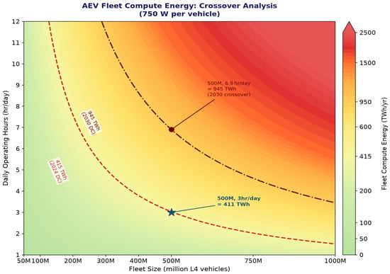
A privately owned automated vehicle may operate autonomously for about one to three hours per day. A robotaxi or logistics vehicle may operate for eight to sixteen hours. The same hardware therefore creates very different annual loads. Figure 4 maps the interaction for the 0.75 kW reference case.

Figure 4. Annual onboard compute electricity as a function of fleet size and daily operating time (0.75 kW reference). Dashed lines mark IEA data centerbenchmarks for 2024 (~415 TWh) and 2030 (~945 TWh) [12]. (The figure retains a rounded 950 TWh line, while the text uses the IEA 945 TWh benchmark. This small difference does not change the main conclusion.)

The 2024 data center energy line is crossed near 505 million vehicles at three hours per day. The 2030 data centerbase case requires about 1.15 billion vehicles at the same duty cycle, or about 6.9 h per day for a 500-million-vehicle fleet. At the near-term scale of 50 million vehicles, commercial operation at 8 h/day yields 109.5 TWh/year—well below the 945 TWh benchmark. Reaching 945 TWh at 8 h/day requires approximately 500 million vehicles (1095 TWh/year), consistent with the long-term era.

5.2. Selected Deployment Cases

Table 8 shows fleet compute electricity and combined fleet electricity for four deployment cases at the reference power level. The fleet sizes and calendar labels are illustrative scenarios, not forecasts or estimated global fleet shares. For scenario identification, the near-term era is associated with approximately 2030, the mid-term era with approximately 2035, and the long-term era with approximately 2040. The 2024 and 2030 data centervalues are historical and prospective reference benchmarks; they are not same-year forecasts for the 2035 or 2040 cases.

Table 8. Fleet-scale annual energy projections. Personal vehicle rows: 3000 kWh/vehicle/yr propulsion and 3 h/day autonomy. Commercial row: 13,140 kWh/vehicle/yr propulsion and 8 h/day. Reference power: 0.75 kW.

Deployment Era	Fleet Size	Compute Electricity (TWh/yr) 0.75 kW, 3 h/day	Propulsion Electricity (TWh/yr) 3000 kWh/Vehicle (Personal Rows; Commercial: 13,140 kWh) †	Combined Fleet (TWh/yr)
Illustration~2030	50 million	41	150	191
Illustration~2035	300 million	246	900	1146
Illustration~2040	500 million	411	1500	1911
Commercial (8 h/day)	100 million	219	1314	1533

† Propulsion baseline of 3000 kWh/yr assumes a personal vehicle traveling ~10,000–14,000 mi/yr (FHWA National Household Travel Survey). For commercial robotaxi or logistics deployments operating at 8 h/day or 10 h/day, annual vehicle mileage substantially exceeds this figure and propulsion energy scales accordingly. The commercial (8 h/day) row uses 13,140 kWh/vehicle/year propulsion, based on 15 mph assumed service speed (43,800 miles/year at 300 Wh/mile). Operators should substitute their actual annual mileage and vehicle efficiency when sizing fleet-level energy budgets. At H = 1 h/day (U.S. average daily driving time per the American Time Use Survey), per-vehicle compute energy is 0.75 × 1 × 365 = 274 kWh/yr; a 50-million-vehicle fleet consumes 13.7 TWh/yr.

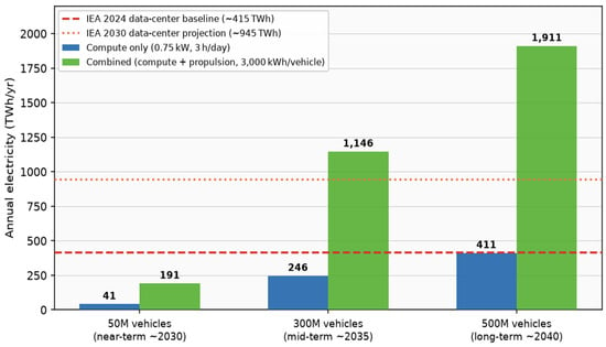
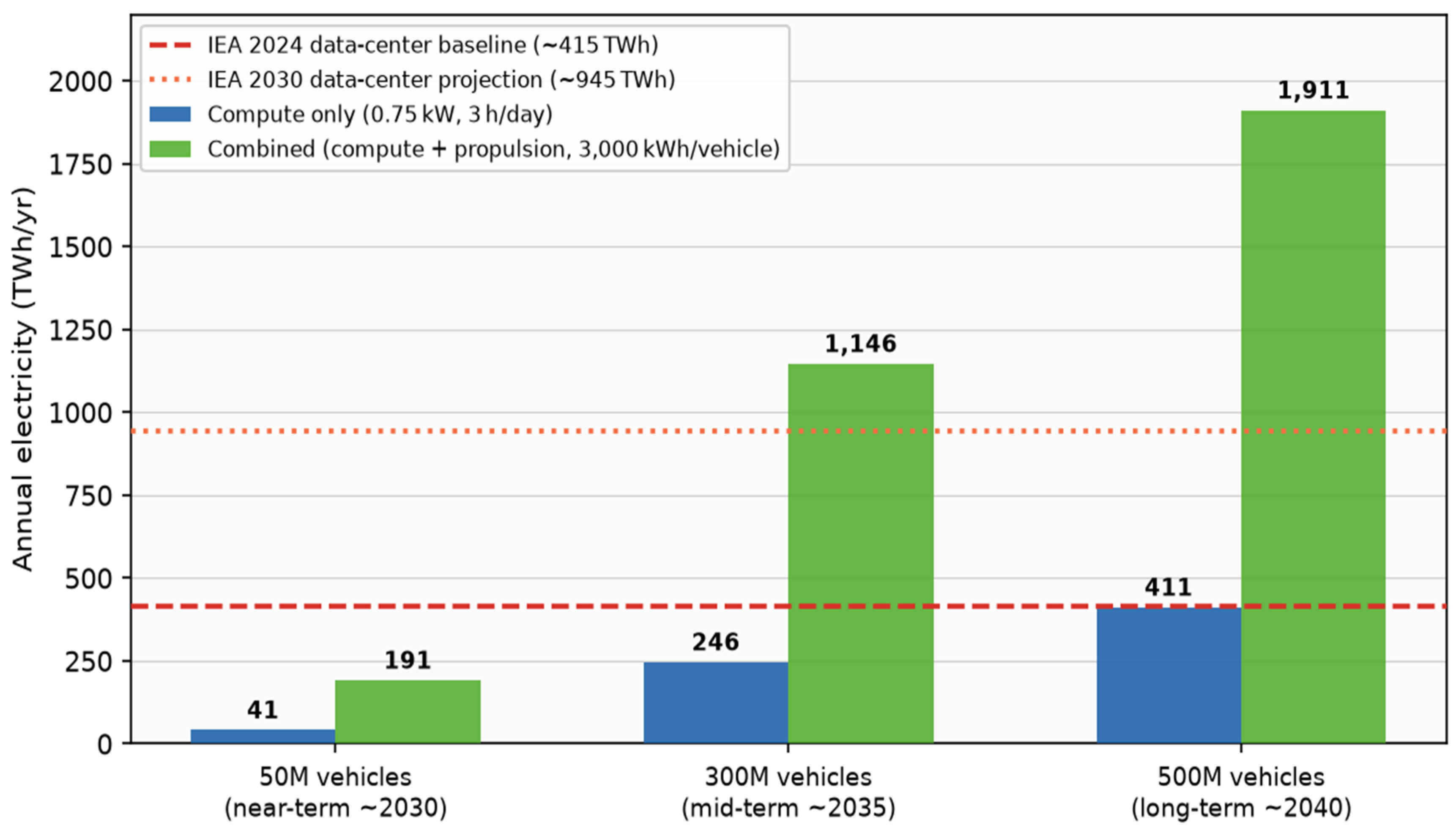
The reference case produces 41 TWh/yr for 50 million vehicles, 246 TWh for 300 million, and 411 TWh for 500 million. As an illustration, although it is not the case today, the long-term compute figure of 411 TWh/yr matches the 2024 global data centerelectricity consumption (~415 TWh). This confirms the ‘data centers on wheels’ characterization, provided the comparison is limited to onboard compute energy. At the long-term scale of 500 million vehicles, commercial operation at 8 h/day reaches approximately 1095 TWh/year—exceeding the IEA projected 2030 data centerbenchmark of ~945 TWh. At the near-term 50-million-vehicle scale, the same duty cycle produces 109.5 TWh/year, well below that threshold. At the 0.75 kW reference, a 500-million-vehicle fleet operating 6.9 h/day matches the 2030 data center projection—a duty cycle consistent with intensive commercial use cases. Figure 5 shows selected fleet compute energy scenarios compared with IEA data center electricity benchmarks.

Figure 5. Selected fleet compute energy scenarios compared with IEA data center electricity benchmarks [12]. Illustration of ~2030 (41 TWh), mid-term (246 TWh), and long-term (411 TWh) cases at 0.75 kW and 3 h/day.

The closest valid comparison is onboard digital electricity versus data center electricity. Adding propulsion to the vehicle total and comparing the result with data centers answers a different question: how much electricity a large electric fleet may use relative to one digital sector. That comparison is useful for grid planning. It should not be presented as evidence that autonomous computing alone exceeds data centers.

The combined fleet comparison in Table 8 separates the two loads before adding them. Cloud training, map production, and communication networks also belong to the full digital footprint, but their energy cannot be inferred from onboard watts. This paper keeps them outside the core model and recommends a separate edge-to-cloud inventory when operational data are available.

6. CO₂ Emission Analysis

Carbon emissions from AEV fleets scale directly with the carbon intensity of the electricity supply. The same hardware produces vastly different emissions depending on whether it charges from coal, gas, nuclear, or renewable sources. This section quantifies those differences and places them in the context of current and projected data centersector emissions.

6.1. Electricity Generation Life-Cycle Emissions

Table 9 uses IPCC AR5 Annex III, Table A.III.2 median life-cycle greenhouse gas factors [27]: pulverized coal 820, combined-cycle gas 490, nuclear 12, utility-scale solar PV 48, and onshore wind 11 g CO₂e/kWh. Emissions are computed from unrounded fleet energy.

Table 9. CO₂ emissions for a 500-million-vehicle L4 AEV fleet (0.75 kW, 3 h/day; combined fleet energy 1910.625 TWh/year). Current data centeroperational CO₂ is approximately 180 Mt/yr [12]. coal (820 g CO₂e/kWh), natural gas (490 g CO₂e/kWh), nuclear (12), solar PV (48), and wind (11 g CO₂e/kWh) values are IPCC AR5 Annex III life-cycle medians. Calculated from unrounded fleet energy.

Generation Technology	Life-Cycle Factor (g CO2e/kWh)	Autonomy Emissions (Mt CO2e/year) 411 TWh	Combined Fleet Emissions (Mt CO2e/year) 1911 TWh	Reduction vs. Coal (%)
Coal (pulverized)	820	336.7	1566.7	0.0%
Natural gas (CCGT)	490	201.2	936.2	40.2%
Nuclear	12	4.93	22.9	98.5%
Solar PV (utility)	48	19.7	91.7	94.1%
Wind (onshore)	11	4.52	21.0	98.7%

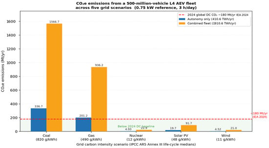
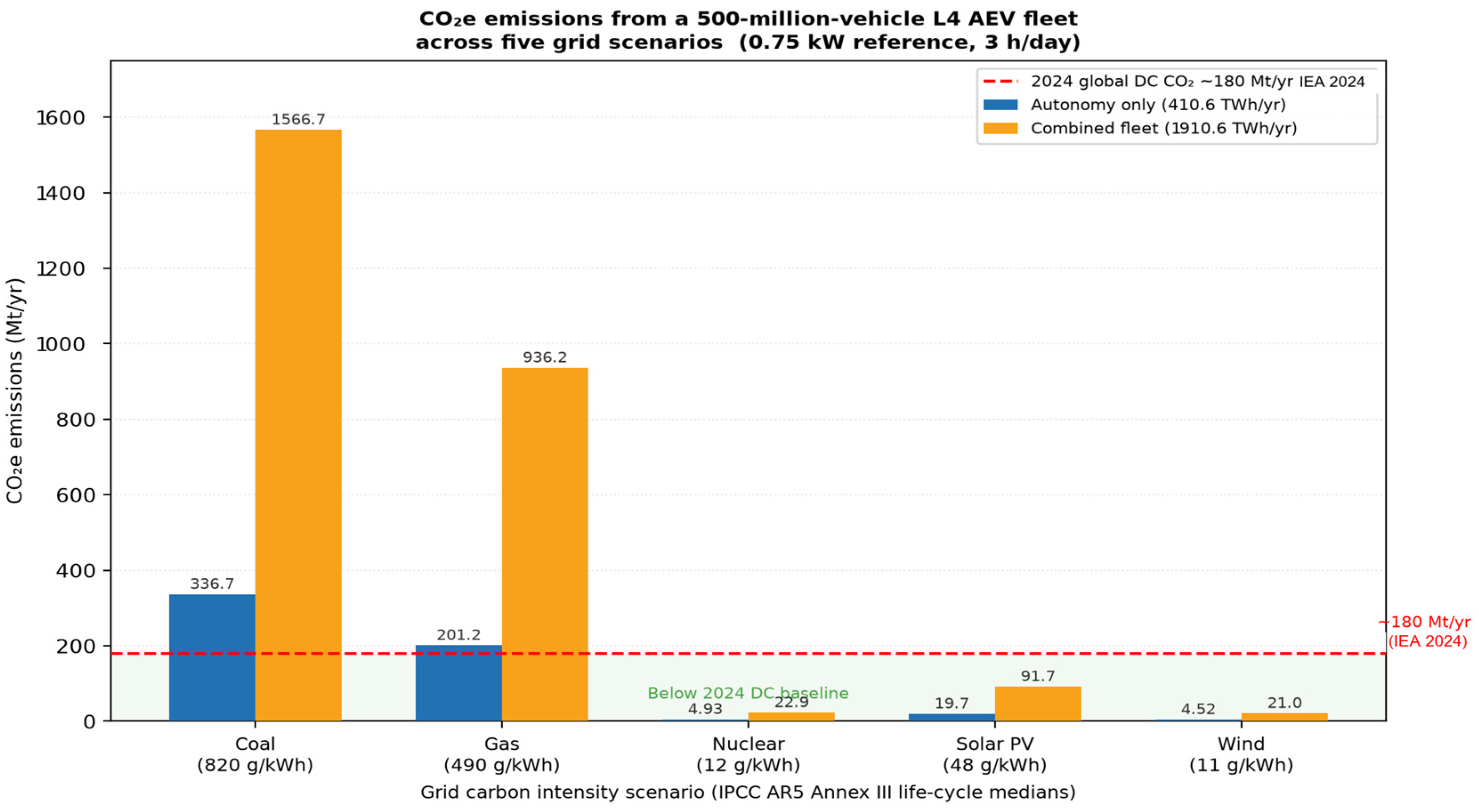
A coal-powered 500-million-vehicle fleet would emit approximately 1566.7 Mt CO₂e/year from combined propulsion and autonomy under coal. The same fleet on wind would emit only 21.0 Mt CO₂e/year (combined propulsion and autonomy)—a 98.7% reduction from coal. Compute-only emissions would be approximately 19.7 Mt CO₂e/year on solar PV and 4.52 Mt CO₂e/year on wind. Grid decarbonization is therefore the single most powerful mitigation lever. Figure 6 plots these five scenarios graphically.

Figure 6. Electricity generation life-cycle CO₂e emissions for the five technologies in Table 9 using IPCC AR5 Annex III medians [27]. Autonomy: 410.625 TWh/year; combined: 1910.625 TWh/year. The ~180 Mt/yr data centre CO₂ benchmark is from IEA [12].

6.2. Operational Emission Comparison

Using the 2024 global power-sector operational intensity of 445 g CO₂/kWh [24], the 410.625 TWh autonomy load corresponds to 182.7 Mt CO₂/year and the combined 1910.625 TWh load to 850.2 Mt CO₂/year. Illustration ~2030 (50 million vehicles, coal grid): approximately 34 Mt CO₂e/yr, comparable to the annual national CO₂ output of Sweden (~44 Mt CO₂ in 2025) or Norway (~36.5 Mt fossil CO₂ in 2025). Illustration ~2035 (300 million vehicles, coal): approximately 202 Mt CO₂e/yr, comparable to Spain (~220 Mt in 2025). Illustration ~2040 (500 million vehicles, coal): ~337 Mt CO₂e/yr. These comparisons underscore that AEV deployment timelines must be synchronized with grid decarbonization roadmaps. These illustrative values apply IPCC AR5 Annex III coal intensity (820 g CO₂e/kWh); for life-cycle comparisons across all five grid technologies, see Table 9 and Figure 6.

7. Autonomous Electric Vehicles as Mobile Data Centers

The combination of high-rate sensing, real-time AI inference, redundant power delivery, and thermal management gives Level 4 vehicles a computational character similar to a distributed edge data center. This section develops that analogy quantitatively, reviews commercial power profiles, and evaluates strategies for improving efficiency at the hardware and fleet levels.

7.1. Architectural Analogy

A Level 4 autonomous electric vehicle combines high-rate sensing, real-time AI inference, redundant power delivery, high-speed networking, storage, and thermal management. These functions resemble a compact edge data center. The vehicle must also satisfy limits on space, weight, vibration, temperature, latency, and functional safety. Both systems contain accelerators, general-purpose processors, memory, storage, high-bandwidth networks, power conversion, and cooling.

The operating environments differ. Data centers aggregate shared workloads at fixed sites with managed cooling. Vehicles distribute smaller real-time systems across a mobile fleet subject to ASIL-D functional safety requirements, automotive temperature ranges (−40 °C to +125 °C), vibration, and 10+ year reliability demands [28,29]. The comparison is useful when the system boundary and operating hours are stated clearly.

7.2. Commercial Deployments: Power Profiles

Publicly disclosed specifications from deployed commercial systems are consistent with the power estimates used in this analysis. Table 10 summarizes the major commercial Level 3/4 deployments.

Table 10. Power profiles of deployed commercial AV systems. Values are estimates based on publicly available disclosures.

System	Deployment	Sensor Count	Est. System Power (W)	Notes
Waymo Driver 1 (5th Gen)	Robotaxi, geofenced	40 (29 cameras, 5 LiDAR, and 6 radar)	~1000–1500	Jaguar I-PACE platform
Zoox 2	Purpose-built L4	150+ sensors	~1000	16 h daily operation
Baidu Apollo RT6 3	Commercial robotaxi	38 sensors	~1000–1500	Production cost-optimized
Mercedes DRIVE PILOT 4	L3 production	30+ sensors	~700–800	Approved for public roads

Notes. ¹ Waymo LLC. “A Look Under Our Trunk: Inside Waymo’s Custom Compute.” Waymo Blog, August 2026. Available: https://waymo.com/blog/2026/08/look-under-our-trunk/(accessed on 5 October 2026). System employs 29 cameras including five LiDAR units and a custom 5 nm ASIC; power estimate based on sensor array and compute specifications. ² Zoox/Amazon. “Sustainable and Attainable: Zoox Unveils Autonomous Robotaxi Powered by NVIDIA.” NVIDIA Blog, December 2020. Available: https://blogs.nvidia.com/blog/2020/12/17/zoox-autonomous-robotaxi-powered-by-nvidia/ (accessed on 5 October 2026). System employs 150+ sensors; power estimate based on NVIDIA Orin compute specifications and 16 h daily operational profile reported by Zoox. ³ Baidu Inc. “Baidu Unveils Next-Gen Autonomous Vehicle Apollo RT6.” Press Release, 21 July 2022. Available: https://ir.baidu.com (accessed on 5 October 2026). RT6 features 1200 TOPS computing platform with 38 sensors including eight LiDAR units; power estimate derived from published compute and sensor specifications. ⁴ Mercedes-Benz. “Automated Driving Revolution: Mercedes-Benz Announces U.S. Availability of DRIVE PILOT.” Mercedes-Benz Media, 2023. Available: https://www.automotiveworld.com/news/automated-driving-revolution-mercedes-benz-announces-u-s-availability-of-drive-pilot-the-worlds-first-certified-sae-level-3-system-for-the-u-s-market/ (accessed on 5 October 2026). DRIVE PILOT adds LiDAR (Valeo Scala 2), redundant cameras, microphones, and a supplemental 12 V backup power subsystem; power estimate based on disclosed sensor and redundancy hardware. The 6th generation (Ojai/Zeekr Van) has 23 sensors (Cameras: 13, LiDAR: 4, Radar: 6).

These deployments consistently show system-level power in the range of 700 W to 1.5 kW. The 700 W–1.5 kW system power range in Table 10 confirms the 0.75 kW reference and brackets the 1.20 kW high-power sensitivity case. The 0.45 kW low-power case represents a projected future efficiency target, not a value drawn from current commercial deployments in Table 10. This supports the technology trend toward advancing performance without increasing power consumption. It is also consistent with Level 4 autonomy historically requiring approximately 1 kW of system power (sensors plus compute) even in earlier multi-chip configurations.

7.3. Quantitative Data Center Comparison

Sudhakar et al. formalized the data centeranalogy and estimated that one billion vehicles at 840 W for one hour per day would emit CO₂ comparable to all global data centers [13]. Two important contextual differences should be noted. First, Sudhakar et al. used Q~0.79 h/day (the 2017 U.S. National Household Travel Survey average); this paper uses Q = 3 h/day for a Level 4 personal AV, plus 8 and 10 h/day commercial scenarios. Second, Sudhakar et al. modeled computer power only (DNN inference); the 750 W reference here includes sensing, networking, conversion, and cooling. Third, the scenarios here use 50, 300, and 500 million vehicles—more conservative than Sudhakar’s 1 billion-vehicle scenario (current global EV fleet: ~80 to 90 million vehicles). Table 11 summarizes the comparison.

Table 11. AEV fleet versus global data centerenergy and CO₂ (data center electricity figures are 2024 values reported by IEA (2025) [12]).

Metric	AEV Fleet (500 M Vehicles, 3 h/day, Power Varies by Row)	Global Data Centers (2024, IEA [12])	Ratio
Compute electricity (TWh/yr), 0.45 kW	246 (compute only)	~415	~0.6×
Compute electricity (TWh/yr), 0.75 kW (reference)	411 (compute only)	~415	~1.0×
Compute electricity (TWh/yr), 1.20 kW	657 (compute only)	~415	~1.6×
Combined fleet electricity (TWh/yr)	1911	~415	~4.6×
Operational CO2, global avg (Mt/yr)	183 (compute)	~180	~1.0×

The long-term compute load of 411 TWh/yr matches the 2024 data center baseline. Laarabi et al. further included cloud AV infrastructure and found the combined footprint substantially larger [22]. Including propulsion, total fleet energy (1911 TWh/yr) exceeds data centerenergy by approximately 4.6×, representing a potential global energy challenge of an entirely different magnitude.

7.4. Hardware Efficiency, Fleet Operation, and V2G

The energy target should be defined at the system level rather than as peak TOPS. Workload-specific accelerators improve performance per watt, but memory transfers, safety processors, networking, conversion losses, and cooling remain. Newer platforms integrate more vehicle functions; so, a lower chip power does not automatically produce a lower vehicle-level load. EcoFusion reported approximately 60% lower energy than comparison methods on its experimental NVIDIA DRIVE PX2 setup while improving object-detection performance in the reported benchmark [30]. That result demonstrates that context-aware sensor selection can remove unnecessary work. It should not be interpreted as a 60% reduction for a complete Level 4 vehicle.

Quantization, pruning, early exits, sparse execution, and reduced-precision arithmetic can lower compute energy [31]. Safety evidence must accompany any approximation that changes the behavior of a perception or planning function. ISO 26262 addresses functional safety for road-vehicle electrical and electronic systems. ISO 21448 addresses safety of the intended functionality when hazards arise from functional insufficiency rather than component failure [29,32]. These standards do not prescribe a fixed power overhead. Architecture-specific measurements should replace generic claims that safety certification doubles power.

Nearly all electrical power consumed by the compute stack becomes heat inside the vehicle. The thermal system therefore needs capacity for average load, transient peaks, hot ambient operation, and degraded cooling modes. A centralized architecture may remove duplicated electronic control units and reduce wiring, but it concentrates heat and increases the consequence of a single failure.

Managed charging can shift propulsion energy away from local demand peaks. Onboard autonomy energy occurs mainly while a vehicle is moving and cannot easily be time-shifted. A commercial fleet may also consume energy while idling with the automated driving system active. Fleet software should record active driving, ready-but-stationary time, charging time, uploaded data, and ambient conditions.

Vehicle-to-grid (V2G) operation can provide grid capacity when many vehicles are parked and connected. Its value depends on connection time, charger capability, battery degradation limits, electricity prices, and local distribution constraints. Life-cycle analyses show fully electrified autonomous taxi fleets on renewables can achieve 70–90% lower lifecycle greenhouse gas emissions than gasoline vehicles [16,20]. Fleet studies should evaluate these conditions before assigning an emission benefit to V2G.

8. Strategies for Energy-Efficient Fleet Autonomy

Reducing fleet energy requires action at multiple levels: more efficient hardware, better workload management, smarter communication strategies, and improved charging coordination. No single measure controls the outcome; different levers address different parts of the energy equation. This section surveys these strategies and organizes them by the metric that verifies their effectiveness.

8.1. Semiconductor Efficiency and Propulsion Effects

Each generation of AI accelerator achieves approximately a 2× improvement in TOPS/W. NVIDIA’s progression from Xavier (~1 TOPS/W in 2018) to Orin (~5 TOPS/W in 2022) and subsequently to Thor (projected > 10 TOPS/W) demonstrates this trend. If 2035–40 chips reach 15 TOPS/W, Level 4 compute at 2000 TOPS could be delivered at approximately 133.3 W—a 76.8% reduction relative to the assumed 575 W computing component of the 0.75 kW budget. Sensors, networking, conversion, and cooling must be addressed separately to achieve full system-level gains. Algorithm-level improvements compound these chip efficiency gains: event-driven sensor fusion and learning-based motion planners have been shown to reduce active compute cycles by 30–45% relative to classical rule-based pipelines [33,34], directly reducing the duty cycle of the computing subsystem and supporting the DVFS-compatible operating assumption in Section 3.2.

Automation can also improve propulsion efficiency through smoother speed control, cooperative driving, optimized routing, and reduced stop-and-go traffic. V2X-enabled traffic signal integration allows vehicles to optimize speed profiles to arrive at green signals, reducing braking and re-acceleration energy. Platoon formation reduces aerodynamic drag across multiple vehicles by 15–25% [14].

Automation can also increase travel by lowering the time cost of a trip and expanding mobility access. Reviews consistently identify travel demand as a major source of uncertainty [14,15,17,18]. A vehicle-level energy improvement can therefore coexist with higher system-level energy use. Electrified autonomous taxis reduce life-cycle emissions when they operate on a decarbonizing grid with high occupancy, long service life, and efficient charging [16,20].

8.2. Communications and Cloud Services

Raw sensor generation does not equal network traffic. Most safety-critical processing must remain local because a vehicle cannot rely on a remote connection for immediate control. Uploaded information may include selected events, compressed logs, maps, diagnostics, and model updates. A credible estimate should report bytes transmitted per vehicle mile, retention time, model-training frequency, network energy intensity, and data center power usage effectiveness [7,21].

The distinction also prevents double counting. If cloud energy already appears in a data center benchmark, adding the same cloud load to the vehicle side and then comparing the total with that benchmark counts part of the digital infrastructure twice. Onboard electricity, network electricity, cloud electricity, and propulsion electricity should be reported as separate rows before any total is formed.

8.3. Integrated Efficiency Roadmap

No single measure controls fleet energy use. Hardware, software, sensing, thermal design, fleet operation, and electricity supply affect different parts of the result. Table 12 organizes efficiency strategies by the quantity that should be verified. The system-level total should be measured after integration because savings in one component can be offset by redundancy, memory traffic, or cooling elsewhere. Efficiency gains reported for the computing component (e.g., 130 W at 15 TOPS/W) should not be applied to the full 0.75 kW system budget without separately accounting for sensor, networking, conversion, and cooling power.

Table 12. Conditional component-based efficiency illustration for a 500 million-vehicle fleet at 3 h/day. Values are author design targets assuming simultaneous achievement; they are not experimentally demonstrated system savings.

Strategy	Verified by	Fleet Impact at 500 M Vehicles (0.75 kW Baseline = 411 TWh)
Advanced chip (15 TOPS/W)	Compute-chip power (W)	Chip ~133 W; system ~308 W → ~169 TWh (−59%)
Solid-state LiDAR + sensor fusion	Sensor power + detection accuracy	~70 W sensing reduction → saves ~38 TWh
DVFS/workload scheduling	Per-task energy (J) + latency (ms)	15% of computing: ~47 TWh saved alone; ~11 TWh after chip improvement
Managed charging (renewable)	Charging schedule + grid intensity	~90% CO2 reduction at same electricity use
Combined (chip + sensor + DVFS)	End-to-end vehicle power (W)	~218 W system (~220 W) → ~120 TWh (−71%)

Table 12 applies efficiency gains to distinct components of the 0.75 kW system boundary. The computing chip currently accounts for the dominant share (~575 W in multi-chip configurations); next-generation AI accelerators at 15 TOPS/W reduce this to 133.3 W (chip power only, at 2000 TOPS/15 TOPS/W). Solid-state LiDAR and event-camera fusion reduce the sensing subsystem from approximately 100 W to 30 W. Dynamic voltage and frequency scaling (DVFS) applies an additional 15% reduction to the computing component alone—throttling it during low-complexity maneuvers—reducing compute from 133.3 W to 113.3 W (133.3 × 0.85). The three-improvement combination gives: 113.3 W compute (post-DVFS) + 30 W sensing + 75 W other loads (memory, networking, power conversion, thermal management) = 218.3 W ≈ 218 W. At this combined target, a 500-million-vehicle fleet would consume approximately 120 TWh/year for onboard autonomy, a 71% reduction from the 410.6 TWh reference case. These efficiency targets represent a technical roadmap goal; the 130 W compute figure is a chip-level projection that must be reconciled with ASIL-D lockstep overhead and thermal management requirements before it translates into a certified production specification.

8.4. Improving Propulsion System Efficiency

Improving overall propulsion efficiency and battery energy density provides a complementary path to reducing the total energy demand of an autonomous electric vehicle. Gains on the propulsion side can partially or fully offset the added compute load, reducing the net impact on range and annual electricity consumption. Recent research has also highlighted zinc-ion hybrid supercapacitors and sustainable electrode materials as emerging energy-storage technologies for EV applications [35,36].

Advanced battery chemistries are raising energy density while reducing cost. Silicon-anode cells are pushing energy density beyond 280 Wh/kg. Solid-state electrolytes are in pilot production, targeting vehicle ranges exceeding 1200 km, with CATL reporting a 1500 km target. Sodium-ion cells with energy density above 200 Wh/kg and a cost target below 45 USD/kWh are projected by 2030. Higher energy density can improve range; it does not independently reduce the autonomy load in kWh. Hence, higher energy density directly offsets the range penalty from the autonomy load without requiring a larger, heavier, or more costly pack. AI-driven battery management systems predict degradation before failure and extend duty-cycle life under fleet operating conditions.

Electric motor and power electronics advances further improve drivetrain efficiency. Rare-earth-light and ferrite motor designs reduce supply chain risk, while axial-flux topologies raise power density. Integrated e-axles that combine the motor, inverter, and gearbox reduce mass and packaging volume. Wide-bandgap semiconductor devices—silicon carbide (SiC) and gallium nitride (GaN)—cut switching losses across the propulsion inverter and on-board charger. According to industry trackers like TrendForce, global SiC inverter penetration entered 2026 for electric vehicles on a steep trajectory after clearing 18% in late 2025 [37]. Higher switching frequencies enabled by SiC and GaN allow for smaller passive components and more compact thermal management, improving overall system efficiency.

Charging infrastructure improvements also affect net energy efficiency. Platforms operating at 800 V enable a charge from 10% to 80% of capacity in approximately 10 to 15 min, reducing idle time for commercial fleets. Megawatt-class chargers are emerging for fleet depots and heavy-duty vehicle applications. Vehicle-to-grid (V2G) capability allows parked vehicles to return stored energy during peak demand, partially recovering the cost of charging and relieving coincident grid stress. Smart managed charging shifts propulsion load away from grid peaks, lowering effective energy cost and reducing coincident demand on distribution networks.

Together, these propulsion-side advances reduce the total per-vehicle energy required per kilometer traveled, increase the fraction of stored energy available for traction, and improve overall system efficiency. They do not eliminate the need for efficient autonomy hardware, but they widen the energy budget within which the compute stack must operate and reduce fleet-level carbon intensity per kilometer. The most effective outcome combines both directions: more efficient compute hardware and more efficient propulsion systems acting together.

9. Challenges and Future Outlook

Wide-scale Level 4 deployment will interact with power grids, battery supply chains, and travel demand in ways that extend well beyond the vehicle-level energy model developed in earlier sections. This section examines those broader challenges, identifies the measurements needed to resolve key uncertainties, and outlines the long-term trajectory under different efficiency and decarbonization scenarios.

9.1. Grid Infrastructure and Fleet Deployment

Large automated fleets add both propulsion and digital demand to the power system. The annual total matters for generation planning, while the time and location of charging determine local capacity needs. Commercial fleets can create concentrated loads at depots, airports, logistics hubs, and urban charging sites. Deployment studies should connect fleet growth with feeder capacity, charging schedules, electricity prices, and regional generation plans.

If Level 4 vehicles reach 300 million units by 2035 while coal still dominates in major markets, the compute energy penalty could negate much of the efficiency gain from electrification. A low-carbon grid reduces operational emissions but does not remove the need for new generation, transmission, distribution, and charging equipment. Fleet deployment and grid decarbonization should be evaluated together while retaining separate metrics for electricity demand and carbon intensity.

9.2. Battery Range and the Full Digital Footprint

Manufacturers can offset an autonomy range penalty by increasing battery capacity, but a larger battery adds mass, cost, charging time, and manufacturing emissions. Improving the autonomy stack avoids part of that tradeoff. With compute consuming approximately 21% of total energy, AEV manufacturers face real pressure to increase battery capacity to maintain range. Reducing compute power through more efficient chips is the more elegant solution.

The full digital footprint extends beyond the vehicle. It includes communication networks, map production, software development, model training, remote assistance, data storage, and fleet management. These services may be important, but their energy cannot be inferred from onboard watts. A complete inventory needs transmitted data per mile, retention time, training frequency, infrastructure utilization, and the electricity supply used by each service [7,21]. Future architectures achieving equivalent fault coverage with lockstep processing at near-threshold voltages could deliver 30–40% power reduction while maintaining safety certification [28,29].

9.3. Measurement and Research Priorities

Table 13 identifies the dominant uncertainties and the measurements needed to resolve them.

Table 13. Dominant uncertainties and recommended measurements.

Uncertainty	Recommended Measurement	Priority
Average system power vs. nameplate	Instrumented vehicle: average + peak watts, duty cycle, speed distribution	High
Sensor power vs. compute power split	Separate sub-metering of sensor, compute, and conversion losses	High
Commercial duty cycle	Fleet telemetry: active hours, ready hours, idle hours	High
Battery degradation under digital load	Cycle testing with autonomy profile vs. propulsion-only	Medium
Cloud + network footprint	Bytes uploaded/mile, training frequency, PUE of serving infrastructure	Medium
Life-cycle emissions vs. grid trajectory	LCA coupled to grid decarbonization scenario	Medium

The highest-value research need is a public, repeatable measurement protocol for automated electric vehicles. Brown et al. provide a useful experimental template [23]. The 2026 VECTOR Phase 1 dataset adds trajectory and energy records for a connected and automated vehicle platform [38]. Future datasets should include modern production-intent hardware, multiple software loads, weather variation, low-speed urban operation, and fail-operational modes.

Scenario studies should publish calculations and use at least two time-matched data centerbenchmarks. The IEA values of 415 TWh in 2024 and 945 TWh in 2030 illustrate why an outdated stationary benchmark can make a future fleet appear larger than it is [12]. U.S. data center reports and global historical studies also show substantial regional and methodological variation [39,40].

A second priority is workload-based benchmarking. TOPS indicates a theoretical operation rate and does not determine energy for a perception, prediction, or planning task. Benchmarks should measure joules per task and deadline miss rate across representative scenes. A third priority is edge-to-cloud accounting that follows selected data from sensing through transmission, storage, training, and model deployment.

9.4. Illustration ~2040 Outlook

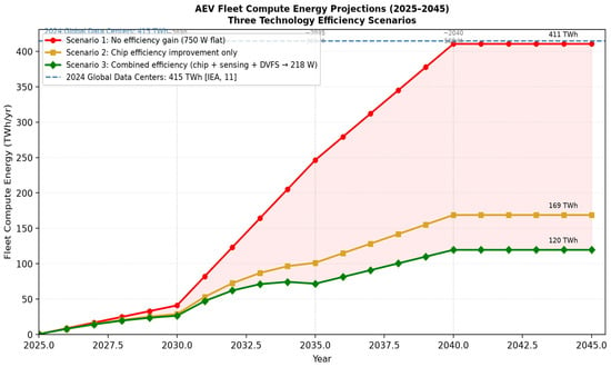
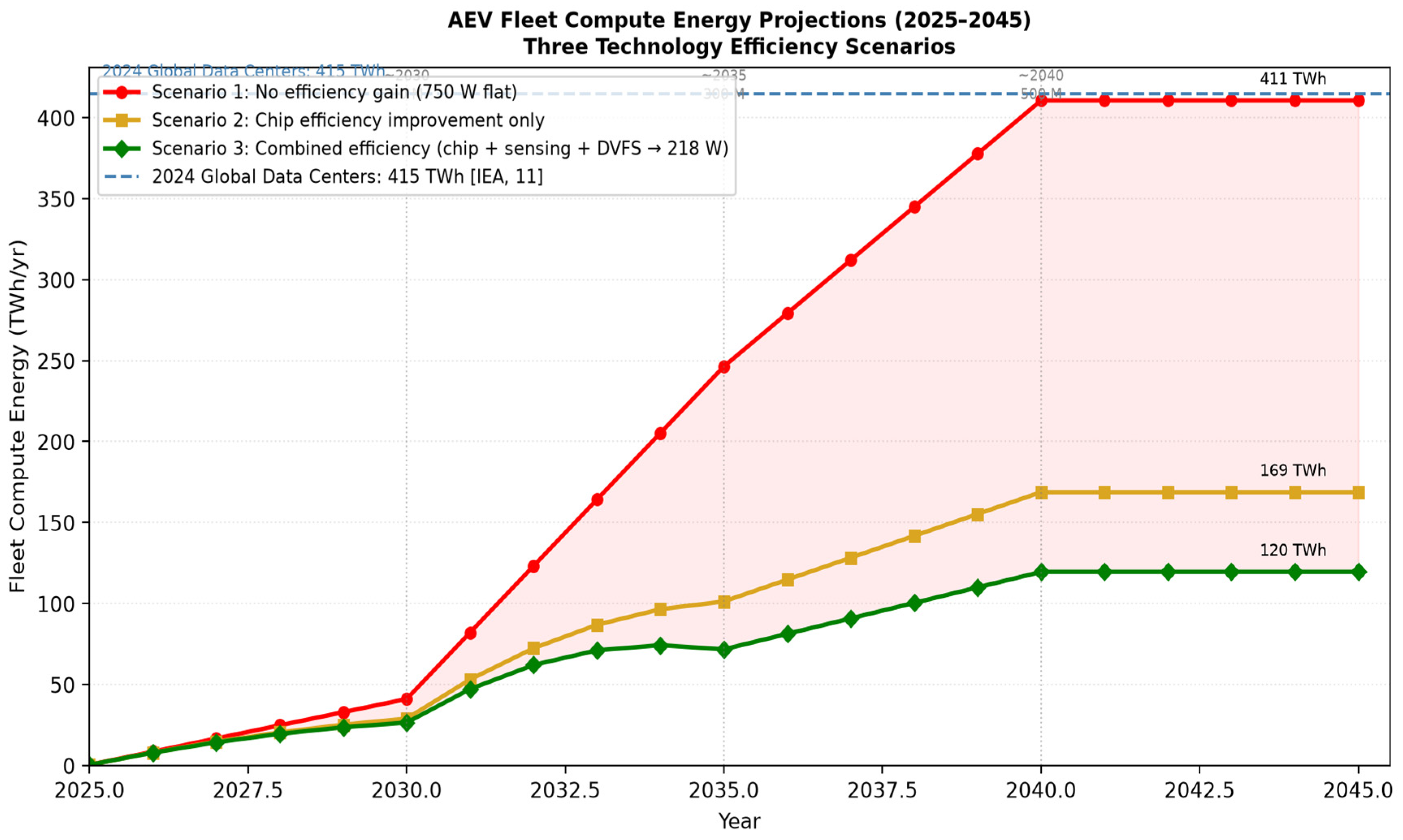
Figure 7 shows fleet compute energy projections from 2025 to 2045 under three scenarios: no efficiency gain (750 W flat), continued chip improvement following historical trends, and combined hardware and software efficiency improvement (chip, sensing, and DVFS).

Figure 7. AEV fleet compute energy projections 2025–2045 under three scenarios: (a) no efficiency gain at 750 W, (b) chip efficiency improvement only, and (c) combined efficiency improvement (chip + sensing + DVFS → 218 W by 2035–40). Fleet sizes are illustrative anchors of 50, 300, and 500 million vehicles at approximately 2030, 2035, and 2040; the intervening trajectory is an illustrative interpolation, with 500 million retained to 2045. These are not IEA or KPMG Level 4 adoption forecasts. Efficiency trajectories follow the Table 12 roadmap. All fleet energy values are compute-only (P × H × N × 365/10⁹, with P in kW and energy in TWh/year), excluding propulsion.

If semiconductor efficiency continues improving at historical rates (approximately 10× per decade), the 2035–40 generation of Level 4 platforms could deliver equivalent compute at 75–150 W for the computing component alone; the full-system roadmap target remains approximately 218 W. Combined with a deeply decarbonized grid, this path converges to a manageable emission trajectory.

The phrase ‘data centers on wheels’ is useful when it draws attention to the computational and thermal character of an automated vehicle. It becomes misleading when the analogy is treated as a fixed equivalence. A vehicle does not operate like a server at constant annual utilization, and a fleet does not share the same location, cooling plant, workload, or grid mix as the data centersector. The comparison is strongest when expressed as a transparent scenario rather than a prediction. The central result is conditional. Five hundred million vehicles at 0.75 kW and three hours per day require 411 TWh/yr, close to global data centerelectricity in 2024. A lower 0.45 kW system uses 246 TWh. A 1.20 kW system uses 657 TWh. The 2030 data centerbase case is not crossed until daily operation approaches seven hours for a 500-million-vehicle fleet. These differences are large enough that the power boundary and duty cycle should appear in every headline claim.

The vehicle result is also conditional. A 0.75 kW load produces a modest range effect at highway speed and a double-digit effect in slow urban service. This makes energy-aware computing especially important for robotaxis, delivery vehicles, shuttles, and other services that combine long operating hours with low average speed. Those are also the services most likely to adopt Level 4 automation as the technology advances.

10. Conclusions

This paper has provided a comprehensive analysis of the energy and emission implications of deploying autonomous electric vehicles at a global fleet scale. The key findings are:

• Onboard autonomy energy deserves its own accounting line. The load includes sensors, networking, power conversion, and incremental cooling—not just the central AI processor—and cannot be inferred from TOPS alone.
• At the reference level (0.75 kW, 3 h/day), compute represents approximately 21.5% of total AEV energy. This is comparable with less than 5% for current Level 2 vehicles.
• A 500-million-vehicle Level 4 fleet generates 411 TWh/yr of compute energy—matching the entire 2024 global data centerconsumption (~415 TWh), confirming the ‘data centers on wheels’ characterization.
• Total fleet energy (propulsion plus compute) reaches 1911 TWh/yr for 500 million vehicles at 3000 kWh/yr propulsion. This exceeds current data centerconsumption by approximately 4.6× and represents a potential global energy challenge of an entirely different magnitude.
• Consistent IPCC AR5 life-cycle factors give combined fleet CO₂e from 1566.7 Mt/year (coal) to 21.0 Mt/year (onshore wind)—a 98.7% reduction for the same 500-million-vehicle fleet.
• Grid decarbonization is the single most impactful lever. Under consistent IPCC AR5 life-cycle factors, replacing coal supply with utility-scale solar PV or onshore wind reduces electricity generation greenhouse gas emissions by 94.1% and 98.7%, respectively. Combined fleet CO₂e falls from 1566.7 to 91.7 (solar PV) and 21.0 Mt/year (wind).
• A fixed autonomy load has a larger range effect at low speed. This is most consequential for robotaxis, urban delivery vehicles, and logistics fleets, which are also the earliest Level 4 adopters.
• Combined technology strategies (advanced chips at 15 TOPS/W, solid-state sensors, and adaptive DVFS) yield a full-system target of approximately 218 W per vehicle (a 71% reduction from 750 W; Table 12). Advanced chip designs alone could target 100–130 W for the compute component by 2035–40.

Autonomous electric vehicles share the computational and thermal character of data centers in meaningful and quantifiable ways—high-rate sensing, real-time AI inference, redundant power delivery, and thermal management. They differ in scale, mobility, duty cycle, and operating environment, and the analogy is strongest when expressed as a transparent, conditional scenario rather than a fixed equivalence. Managing that footprint requires hardware efficiency, software optimization, renewable energy sourcing, and policy coordination. These are the same tools the data centerindustry has developed over the past two decades, now applied at the scale of the global vehicle fleet.

References

- SAE Standard J3016_202104; Taxonomy and Definitions for Terms Related to Driving Automation Systems for On-Road Motor Vehicles. SAE International: Warrendale, PA, USA, 2021. [Google Scholar] [CrossRef] [Scilit]
- Talpes, E.; Gorti, A.; Sachdev, G.S.; Das Sarma, D.; Venkataramanan, G.; Bannon, P.; McGee, B.; Floering, B.; Jalote, A.; Hsiong, C.; et al. Compute Solution for Tesla’s Full Self-Driving Computer. IEEE Micro 2020, 40, 25–35. [Google Scholar] [CrossRef] [Scilit]
- Rajashekara, K.; Koppera, S. Data and Energy Impacts of Intelligent Transportation—A Review. World Electr. Veh. J. 2024, 15, 262. [Google Scholar] [CrossRef] [Scilit]
- Rajashekara, K. Energy Impacts of Autonomous Vehicles—Present and the Future. iEnergy 2024, 3, 73–74. [Google Scholar] [CrossRef] [Scilit]
- Lin, S.C.; Zhang, Y.; Hsu, C.H.; Skach, M.; Haque, M.E.; Tang, L.; Mars, J. The Architectural Implications of Autonomous Driving: Constraints and Acceleration. In Proceedings of the ASPLOS 2018, Williamsburg, VA, USA, 24–28 March 2018; pp. 751–766. [Google Scholar] [CrossRef] [Scilit]
- Fayyad, J.; Jaradat, M.A.; Gruyer, D.; Najjaran, H. Deep Learning Sensor Fusion for Autonomous Vehicle Perception and Localization: A Review. Sensors 2020, 20, 4220. [Google Scholar] [CrossRef] [Scilit] [PubMed]
- Liu, S.; Liu, L.; Tang, J.; Yu, B.; Wang, Y.; Shi, W. Edge Computing for Autonomous Driving: Opportunities and Challenges. Proc. IEEE 2019, 107, 1697–1716. [Google Scholar] [CrossRef] [Scilit]
- NVIDIA. NVIDIA DRIVE AGX Thor Platform for Developers Spec Overview. Available online: https://developer.download.nvidia.com/drive/docs/nvidia-drive-agx-thor-platform-for-developers.pdf (accessed on 1 September 2025).
- NVIDIA. In-Vehicle Computing for Robotaxis and Autonomous Vehicles. Available online: https://www.nvidia.com/en-us/solutions/autonomous-vehicles/in-vehicle-computing/ (accessed on 1 September 2025).
- Qualcomm Technologies. Qualcomm Accelerates Autonomous Driving with New Snapdragon Ride Platform. Available online: https://www.qualcomm.com/news/releases/2020/01/qualcomm-accelerates-autonomous-driving-new-platform-qualcomm-snapdragon (accessed on 1 September 2025).
- Mobileye. New Mobileye EyeQ Ultra Will Enable Consumer AVs. Available online: https://ir.mobileye.com/news-releases/news-release-details/new-mobileye-eyeq-ultra-will-enable-consumer-avs (accessed on 1 September 2025).
- International Energy Agency. Energy and AI; IEA: Paris, France, 2025; Available online: https://www.iea.org/reports/energy-and-ai (accessed on 1 September 2025).
- Sudhakar, S.; Sze, V.; Karaman, S. Data Centers on Wheels: Emissions From Computing Onboard Autonomous Vehicles. IEEE Micro 2023, 43, 29–39. [Google Scholar] [CrossRef] [Scilit]
- Wadud, Z.; MacKenzie, D.; Leiby, P. Help or Hindrance? The Travel Energy and Carbon Impacts of Highly Automated Vehicles. Transp. Res. Part A 2016, 86, 1–18. [Google Scholar] [CrossRef] [Scilit]
- Taiebat, M.; Brown, A.L.; Safford, H.R.; Qu, S.; Xu, M. A Review on Energy, Environmental, and Sustainability Implications of Connected and Automated Vehicles. Environ. Sci. Technol. 2018, 52, 11449–11465. [Google Scholar] [CrossRef] [Scilit] [PubMed]
- Gawron, J.H.; Keoleian, G.A.; De Kleine, R.D.; Wallington, T.J.; Kim, H.C. Deep Decarbonization from Electrified Autonomous Taxi Fleets: Life Cycle Assessment and Case Study in Austin, TX. Transp. Res. Part D 2019, 73, 130–141. [Google Scholar] [CrossRef] [Scilit]
- Morrow, W.R., III; Greenblatt, J.B.; Sturges, A.; Saxena, S.; Gopal, A.; Millstein, D.; Shah, N.; Gilmore, E. Key Factors Influencing Autonomous Vehicles’ Energy and Environmental Outcome. In Road Vehicle Automation; Springer: Cham, Switzerland, 2014. [Google Scholar] [CrossRef] [Scilit]
- Kopelias, P.; Demiridi, E.; Vogiatzis, K.; Skabardonis, A.; Zafiropoulou, V. Connected and Autonomous Vehicles—Environmental Impacts—A Review. Sci. Total Environ. 2020, 712, 135237. [Google Scholar] [CrossRef] [Scilit] [PubMed]
- Liu, F.; Zhao, F.; Liu, Z.; Hao, H. Can Autonomous Vehicles Reduce Greenhouse Gas Emissions? A Country-Level Evaluation. Energy Policy 2019, 132, 462–473. [Google Scholar] [CrossRef] [Scilit]
- Greenblatt, J.B.; Saxena, S. Autonomous Taxis Could Greatly Reduce Greenhouse-Gas Emissions of U.S. Light-Duty Vehicles. Nat. Clim. Change 2015, 5, 860–863. [Google Scholar] [CrossRef] [Scilit]
- van Oosterhout, R.; Striekwold, P.; Wang, M. On Data-Induced CO2 Emissions of Vehicle Automation: An Overlooked Emission Source. Sustain. Horiz. 2024, 9, 100082. [Google Scholar] [CrossRef] [Scilit]
- Laarabi, H.; Kirchstetter, T.; Zuberi, M.J.; Smith, S.J.; Shehabi, A. The Overlooked Energy Footprint of Vehicle Automation from Edge to Data Center Computing. SSRN 2026. [Google Scholar] [CrossRef] [Scilit]
- Brown, N.; Motallebiaraghi, F.; Rojas, J.; Ayantayo, S.; Meyer, R.; Asher, Z.; Ekti, A.R.; Wang, C.; Goberville, N.; Feinberg, B. Evaluation of Autonomous Vehicle Sensing and Compute Load on a Chassis Dynamometer. In Proceedings of the 26th IEEE International Conference on Intelligent Transportation Systems (ITSC), Bilbao, Spain, 24–28 September 2023; pp. 1989–1995. [Google Scholar] [CrossRef] [Scilit]
- International Energy Agency. Electricity 2025; IEA: Paris, France, 2025; Available online: https://www.iea.org/reports/electricity-2025/emissions (accessed on 1 September 2025).
- Fiori, C.; Ahn, K.; Rakha, H.A. Power-Based Electric Vehicle Energy Consumption Model. Appl. Energy 2016, 168, 257–268. [Google Scholar] [CrossRef] [Scilit]
- Weiss, M.; Winbush, T.; Newman, A.; Helmers, E. Energy Consumption of Electric Vehicles in Europe. Sustainability 2024, 16, 7529. [Google Scholar] [CrossRef] [Scilit]
- IPCC. Climate Change 2014: Mitigation of Climate Change. Contribution of Working Group III to the Fifth Assessment Report of the Intergovernmental Panel on Climate Change; Cambridge University Press: Cambridge, UK, 2014. [Google Scholar]
- Lo Bello, L.; Mariani, R.; Mubeen, S.; Saponara, S. Recent Advances and Trends in On-Board Embedded and Networked Automotive Systems. IEEE Trans. Ind. Inform. 2019, 15, 1038–1051. [Google Scholar] [CrossRef] [Scilit]
- ISO 26262; Road Vehicles—Functional Safety. International Organization for Standardization (ISO): Geneva, Switzerland, 2018.
- Malawade, A.V.; Mortlock, T.; Al Faruque, M.A. EcoFusion: Energy-Aware Adaptive Sensor Fusion for Efficient Autonomous Vehicle Perception. In Proceedings of the 59th ACM/IEEE DAC, San Francisco, CA, USA, 10–14 July 2022; pp. 481–486. [Google Scholar] [CrossRef] [Scilit]
- Katare, D.; Perino, D.; Nurmi, J.; Warnier, M.; Janssen, M.; Ding, A.Y. A Survey on Approximate Edge AI for Energy Efficient Autonomous Driving Services. IEEE Commun. Surv. Tutor. 2023, 25, 2714–2754. [Google Scholar] [CrossRef] [Scilit]
- ISO 21448; Road Vehicles—Safety of the Intended Functionality. International Organization for Standardization (ISO): Geneva, Switzerland, 2022.
- Chen, Y.; Li, Y.; Wang, X.; Zhang, Z. Event-Driven Sensor Fusion for Autonomous Vehicles: Reducing Compute Cycles via Adaptive Sampling. IEEE Trans. Autom. Sci. Eng. 2025, 22, 1845–1858. [Google Scholar]
- Cai, J.; Liu, M.; Chen, H.; Zhao, W. Safety-Region-Based Motion Planning with Learning-Based Prediction for Autonomous Driving. IEEE Trans. Transp. Electrif. 2025, 11, 3201–3214. [Google Scholar]
- Mohamed, M.M.; Aziz, M.A.; Hussain, A.; Hardianto, Y.; Yamani, Z. Dendrite-Free Zinc-Ion Hybrid Supercapacitor with Jute-Derived Carbon and Nanostructured Zinc on Steel Mesh for EVs. J. Energy Storage 2024, 100, 113635. [Google Scholar] [CrossRef] [Scilit]
- Abdolrasol, M.G.M.; Ansari, S.; Sarker, I.A.; Tiong, S.K.; Hannan, M.A. Lithium-ion to sodium-ion batteries transitioning: Trends, analysis and innovative technologies prospects in EV application. Prog. Energy 2025, 7, 022007. [Google Scholar] [CrossRef] [Scilit]
- TrendForce Corporation. “SiC Power Devices in EV Applications Surpass 18% Penetration in Late 2025.” TrendForce Research, Taipei, Taiwan, January 2026. Available online: https://www.trendforce.com/presscenter/news/20260109-12872.html (accessed on 20 October 2026).
- Ma, K. VECTOR Phase 1 Dataset: CAV Trajectory and Energy Consumption Records; U.S. Department of Energy Data Explorer: Washington, DC, USA, 2026. Available online: https://livewire.energy.gov/ds/vector/phase-1 (accessed on 20 October 2026). [CrossRef]
- Shehabi, A.; Newkirk, A.; Smith, S.J.; Hubbard, A.; Lei, N.; Siddik, M.A.B.; Holecek, B.; Koomey, J.; Masanet, E.; Sartor, D.; et al. 2024 United States Data Center Energy Usage Report; Lawrence Berkeley National Laboratory: Berkeley, CA, USA, 2024. [Google Scholar] [CrossRef]
- Masanet, E.; Shehabi, A.; Lei, N.; Smith, S.; Koomey, J. Recalibrating Global Data Center Energy-Use Estimates. Science 2020, 367, 984–986. [Google Scholar] [CrossRef] [Scilit] [PubMed]
Disclaimer/Publisher’s Note: The statements, opinions and data contained in all publications are solely those of the individual author(s) and contributor(s) and not of MDPI and/or the editor(s). MDPI and/or the editor(s) disclaim responsibility for any injury to people or property resulting from any ideas, methods, instructions or products referred to in the content. |
© 2026 by the author. Published by MDPI on behalf of the World Electric Vehicle Association. Licensee MDPI, Basel, Switzerland. This article is an open access article distributed under the terms and conditions of the Creative Commons Attribution (CC BY) license.