


Abstract
Accurate estimation of state-of-charge (SoC) and state-of-health (SoH) is important for lithium-ion battery operation. This study investigates an actor–critic formulation of joint SoC/SoH estimation using TD3 and SAC with a composite reward and compares the observed results with four supervised baselines. On the supplied XJTU run, the actor–critic models achieved lower observed SoC RMSE than the supervised baselines, while the best supervised model remained competitive or superior for SoH. The current evaluation uses a limited cell cohort and three random seeds, and the per-cell normalization and the OCV calibration used the records of held-out cells (the protocol is not training-only); therefore, the results are exploratory and do not establish confirmatory statistical superiority or generalization to a larger battery population. The planned Tsinghua label-retention experiment could not be completed because the supplied capacity field had no usable variance. The resulting Tsinghua analysis is limited to label-free output diagnostics and does not establish target-domain estimation accuracy or validate reward-model transfer under label scarcity. The reward terms, including a coulomb-counting term applied to SoH that is provisional and not a validated physical constraint, are exploratory, and any mechanistic explanation of the SoC–SoH difference is a hypothesis rather than an established result. The reward-component ablation, the hyperparameter-sensitivity analysis, the matched non-RL comparison, and the Tsinghua label-retention sweep remain future validation requirements.
1. Introduction
Real-time estimation of state of charge (SoC) and state of health (SoH) is important for the safe, efficient, and durable operation of lithium-ion batteries in electric vehicles and stationary storage. SoC describes available charge relative to a defined reference capacity, whereas SoH is commonly related to remaining usable capacity relative to nominal or initial capacity. Although the two quantities are coupled through electrochemical and degradation dynamics, they are not interchangeable and require clearly defined labels, state variables, and evaluation protocols [1,2].
Supervised deep learning has developed the most adopted approach in this area. Various types of artificial neural network architectures, including recurrent networks, attention-based architectures, and temporal–convolutional architectures have been used to predict SoC and SoH based on sequences of voltage, current, and temperature [3,4,5]. Physics-informed approaches are introduced to improve understanding and stability of these models by using constraints describing degradation processes within their loss functions [6,7]. The use of domain adaptation methods, such as CORAL, which allows data collected in laboratory experiments to train models to work with field data, is also observed [8,9]. Several recent studies show the effectiveness of using physics-informed Transformers with temporal convolutional architecture in this aspect [10].
Although there has been advancement, most of the literature addresses estimation SoC or SoH as static or sliding-window regression problems, in which a segment of component sensor history is observed, and a singular point estimate is returned. In this context, the idea that the decision process consists of several consecutive steps and leads to the desired results is absent; the only goal here is lowering the pointwise error. The situation regarding the use of reinforcement learning (RL) for battery management tasks is the opposite, as RL has managed to achieve success in various control tasks, such as charging scheduling, thermal management, and energy dispatching, all of which are characterized by a series of actions whose effects evolve in time [11,12,13].
This gap creates a question that has not been systematically tested until now. Can the task of estimation itself be redefined in terms of a Markov decision process (MDP) where an actor–critic agent acquires SoC/SoH estimates generated as an outcome of a reward signal? This question must be articulated as a genuine, verifiable question rather than as a hypothetical enhancement of the basic concept. The use of an RL approach does not automatically mean that it is more suitable for making such continuous-valued estimations than a supervised regression. It should be noted that actor–critic techniques were originally designed for control tasks, where the agent has an opportunity to affect its future observations. This, however, is impossible in the case of a passive estimating agent working with fixed input data stream. Any proposed advantage has to be proved practically compared with reliable results of methods based on supervised learning rather than presumed from the success of reinforcement learning in similar applications [14].
When we talk about actor–critic techniques, out of the two most used algorithms for continuous action spaces, one is called Twin Delayed Deep Deterministic Policy Gradient (TD3) [15], whereas the other one goes by the name of Soft Actor–Critic (SAC) [16]. Both have their roots in the deep deterministic policy gradient (DDPG) family [17], with the double Q-learning [18] algorithm serving as an even more distant relative to both TD3 and SAC. The TD3 algorithm helps create two critic networks that stabilize the generated value evaluations so as to be low-variance and reliable when solving the continuous output problem. Of note is that the SAC framework uses the entropy principle to promote exploration, which is not as necessary when the decision-making process is limited to a single number as it is when one has a chance to pick between multiple actions. This insight enables one to recognize TD3 as the key algorithm while the SAC algorithm is seen as a means of comparison, thereby confirming that establishing the choice between the deterministic and max entropy actor–critic approaches is not an automatic process [18].
The research discussed in this paper applies to a joint estimation model for SoC/SoH, where it conceptualizes the estimation task as an MDP. It then trains TD3 and SAC agents with a composite reward and describes, as an intended but not yet validated extension, a reward-based transfer procedure for label-scarce field applications that is analogous in purpose to the supervised domain-adaptation approaches in [9,10,11]. The experiments are performed using the XJTU run-to-failure dataset [19] as well as a real-world dataset describing EV battery cycles [20]. A third dataset from CALCE [21] is held out entirely from training and used only to test cross-dataset generalization. The supervised baseline was run using the same data splits as those used for the RL experiment, and the results of RL are compared against those of supervised techniques beforehand, with the conditions mentioned above, which define the success metrics to be applied to RL and supervised methods and help in identifying zero results, situations where RL-based methods did not demonstrate better performance than supervised regressions.
The contributions of this work are as follows: (i) an exploratory formulation of joint SoC/SoH estimation as a sequential decision-making problem; (ii) an exploratory investigation of a physics-motivated reward combining a labeled-error term with consistency terms, in which the coulomb-counting term is evaluated in an alternative SoH-based configuration and is given in its SoC-based form in Equation (19); (iii) a description of an intended reward-model transfer procedure, for which only label-free diagnostics could be obtained, so that its validation remains a future requirement; and (iv) an evaluation on the supplied XJTU run and CALCE dataset that identifies both promising SoC results and important limitations. The present study does not establish that actor–critic learning is intrinsically preferable to direct supervised or self-supervised optimization, nor does it validate reward-model transfer under graded target-domain label scarcity. The reward-component ablation, the hyperparameter-sensitivity analysis, the matched non-RL comparison on the identical composite objective, and the Tsinghua label-retention sweep are future validation requirements; accordingly, no conclusion is drawn here about the relative contribution of individual reward terms or about any advantage specific to actor–critic optimization.
2. Related Work
2.1. Supervised Deep Learning Lineage for SoC/SoH Estimation
In the last ten years, supervised sequence regression has been recognized as the main method used for estimating lithium-ion battery state. Previous studies showed the ability of deep convolutional and recurrent neural networks to SoC given the history of temperature, current, and voltage without using any electrochemical or equivalent-circuit model, showing feasibility under the evaluated conditions [3]. Efforts of scientists have gone further; now, the method is used for predicting the stage of degradation and remaining useful life of the batteries. Thanks to comprehensive datasets, scientists now can create models that function based on early-cycle data without depending on designed health indicators [5].
On the more recent end of the line, however, the lineage is moving towards hybrid systems that combine TCNs and attention/Transformer blocks to account for both the dynamic and long-range aspects of the degradation trend. Specifically, Chen et al. [1] introduced a TCN–Transformer fusion approach to pack-level SoH estimation, tested on real-world operational data [1] and other attention-based approaches, informed by physics of the process, to the same end [8]. This is part of the growing trend of PINNs, where the underlying governing equations or constraints are added as soft penalties in supervised learning, rather than being found by the model [6], an idea that has already been proven viable at scale for battery degradation prognosis [19]. As for the immediate precedent of the current work, it extends the fusion and physics-informed lineage of approaches yet another step forward by including cross-domain feature alignment for transfer between domains [7]. It also introduces the architecture evaluated in this paper: a physics-informed Transformer–TCN with CORAL-based domain adaptation for SoH and RUL estimation across the XJTU and Tsinghua datasets [11]. Systematic studies of such a path validate that almost all advances, fusion architectures, attention mechanisms, physical priors on losses, and adaptation layers, have been made in the context of one and the same paradigm of supervised regression, where the estimator is optimized with respect to a pointwise loss function, relative to the ground truth SoC/SoH values [2,4]. An open question, however, has been to what extent a completely novel paradigm of learning, one that maximizes the reward signal over the entire trajectory, would be advantageous in this estimation task.
2.2. The Gap: Reinforcement Learning in Battery Management
RL has, at the same time, successfully been applied to battery-related decision problems, albeit mainly to control-scheduling rather than state estimation. The application of RL is well documented in the context of EV charging management and scheduling, where learning an optimal charging policy allows the agent to meet various objectives related to the grid or cost [12,13], as well as energy storage and PV control problems, where the action space involves power dispatch or connection rather than actual state estimation [14]. While deep deterministic and stochastic actor critic methods (DDPG, TD3, SAC) were made for precisely this kind of continuous control problem [15,16,17], based on the developments of the value estimation technique including double Q-learning [18], it is worth mentioning that the domain of batteries has made use of these ideas. Namely, DDPG agents have been implemented to optimize EV energy consumption with reference to health-consciousness [14], while deep reinforcement learning (DRL) scheduling has been applied for prolonging the service life of retired EV battery packs using an optimum cell connection/disconnection policy [22].
Whereas RL has impacted state estimation more generally through its indirect effect on filter parameter tuning, most work in this area has been limited to this indirect influence, not using RL as the estimator. RL-tuned adaptive unscented and extended Kalman filters have been suggested for the task of simultaneous SoC/SoH estimation, where RL’s action is the tuning of the filter’s parameters, and not the direct SoC or SoH estimation [23,24]. A similar approach was followed for estimating SoH using a hybrid PPO-corrected LSTM, in which RL acts as an additional step to post-processing the estimation output of a supervised neural network under monotonic degradation constraint [25]. There have been some efforts to use actor–critic algorithms (DDPG) to estimate and jointly control EV batteries’ SoC under varying conditions like torque and temperature [26], as well as recent attempts to propose a control-oriented deep RL approach to Li-ion state estimation that is explicitly adaptive [27]; however, each of these cases uses only one algorithm without any systematic comparison between actor–critic variations, and without a strong physics-based supervised baseline of the kind prevalent in the SoH literature [1,7,8,11]. To the best of our systematic search, researchers have never compared the deterministic policy gradient approach to the maximum entropy stochastic case, TD3 versus SAC, when it comes to continuous SoC/SoH regression. This is surprising, because these two methods show opposite tendencies (determinism and exploitation, on the one hand, and stochasticity and exploration on the other) that directly affect whether RL is suitable for precision estimation tasks.
2.3. Domain Adaptation Contrast
The method of lab-to-real transfer used by the reference architecture follows the prevailing method for domain adaptation used in this literature: match the statistics of the feature space distributions of the source and target domains either with a second-order moment penalty, as in the case of CORAL [9], or an adversarial feature alignment task as in domain adversarial neural networks [10], and train the estimator in conjunction with the matched representation [7,11]. The assumption here is that transferability depends on learned feature space embedding, and the supervised loss should be defined in the target domain.
An actor–critic formulation alters the nature of the object that can be transferred. Instead of matching the distribution of intermediary features, the reward formulation itself, formulated in terms of consistency with open-circuit-voltage relationships, monotonically decreasing capacity fade, or coulomb-counting constraints, in principle, become an object that is transferred, independent of the state formulation learned by the policy network. This shifts the transfer of domains to the transfer of rewards, a fundamentally different approach from CORAL formulations, one that has yet to be investigated in label-scarce field operation of battery estimators. This is a hypothesis that motivates the present study; it is not validated by the experiments reported here.
2.4. Gap Statement
Both lines of research, supervised learning and RL, indicate that significant advances in architecture have led to improved accuracy of SoC and SoH estimations through regression methods. In the context of supervised learning, methods such as hybrid architecture, attention mechanisms and physics-informed losses have been shown to contribute to improvement in SoC/SoH estimation accuracy [1,7,8,11]. In the context of RL, actor–critic architectures have been effective for battery-related control and scheduling problems [12,13,14,22], which now presents only sporadic and limited attempts at applying RL for estimation [23,24,25,26,27]. In fact, to our knowledge, there have been no studies that compare a deterministic actor–critic method (TD3) approached from the perspective of physics-informed methodology against supervised methods, as well as investigate whether reward mechanism for transferring knowledge can replace feature alignment method, while labels are lacking.
The methodological focus of this study is the integration of physics-motivated reward design with actor–critic-based joint state estimation. TD3 and SAC provide two established learning mechanisms for examining this formulation; the central design question is whether the reward combines labeled estimation error with physically motivated consistency constraints in a way that supports reliable SoC and SoH estimation. A further question is whether this reward formulation remains useful when transferred to a domain with limited target labels. These are separate questions: the source-domain estimation results can be evaluated using the available labels, whereas the transfer claim requires a valid target-domain evaluation.
3. Problem Formulation and Methodology
This section describes the estimation of SoC/SoH as a sequential decision-making problem and builds the methodology based on it. By discussing MDPs and two actor–critic algorithms in one part and not separating the “method formulation” from the “method”, this allows us to keep state, action, and reward definitions slipstreamed throughout the text, while the derivations for the TD3 and SAC are built under these definitions.
3.1. MDP Formalization of Joint SoC/SoH Estimation
In contrast to the existing approach of treating the SoC/SoH estimation problem as a static mapping between a window of measurements to a scalar label using supervised regression [3,8], we propose formulating it as a discrete-time Markov Decision Process (MDP) over a finite horizon.
where S is the observation space, A is the continuous action space of joint state estimates, P is the state-transition kernel, R is the reward function, and γ ∈ (0,1] is the discount factor. At each timestep t, the agent observes
composed of the terminal voltage, the current, the temperature of the cell surface, the rate of change over a short period, and the joint estimate of the agent itself from the previous period, respectively, serving as the state. The action is the joint estimate,
This two-dimensional action can be classified as a continuous action, meaning we can use actor–critic methods that utilize continuous space instead of discrete-action value methods. Another aspect of this setup, which sets this action apart from its control applications in the battery literature [12,13,14,24], is that the exogenous measurement kernel is independent of the action (see the clarification below):
The action-independent transition kernel is an important limitation of the present formulation. Unlike a conventional control problem, the estimated SoC/SoH values do not change the battery’s physical state or the subsequent voltage, current, and temperature measurements. The sequential formulation is used here to investigate whether cumulative reward optimization, together with the previous estimate included in the observation, can improve estimation consistency over a recorded trajectory. It does not establish that the estimation problem intrinsically requires an MDP. In particular, the action-independent dynamics also make a contextual bandit or a direct sequence-regression formulation plausible alternative. The suitability of the MDP formulation must therefore be judged by its empirical performance and computational cost relative to these alternatives, rather than by its formal representation alone.
For clarity, let xt = [ Vt, It, Tt, ΔTt] denote the exogenous battery-measurement component of the state, so that st+1 = [xt+1, at]. Equation (4) then holds for the exogenous component, P(xt+1 | st, at) = P(xt+1 | st), whereas the lagged-estimate component of the full state is updated deterministically from the action. The full state transition is therefore not strictly action-independent: the agent’s estimates affect only the lagged-estimate input and the reward, never the measured signals. The current experiments do not include a matched non-RL model trained directly on the identical composite objective, so any advantage specific to actor–critic optimization has not been established and remains a future validation requirement.
The subsequent voltage/current/temperature observation is dependent on the actual physical path that the battery follows as seen in XJTU and Tsinghua datasets, but not on what the agent infers. The estimator cannot affect the process which it is estimating, but only the reward associated with every given estimate. This is how the reward function disconnected from the transition dynamics and becomes the object which supports the physics-based structure (Section 3.4) and is the object which is passed from one domain to another (Section 3.5). The aim of the agent is to receive a maximum discounted return.
where the actor–critic pair is optimized based on maximizing J(π) using trajectories τ generated from cycling data instead of interacting with the physical cell, thus using a more offline fixed batch RL approach similar to the classic treatment of MDP by [28] than the online control applications of RL in battery systems.
3.2. TD3 Formulation and Rationale
The Twin Delayed Deep Deterministic policy gradient (TD3) [15] algorithm is chosen as the main solver for the problem due to the fact that the biases of this approach correspond to the ones that are expected to be seen in a task of this type: the deterministic actor allows eliminating the noise inherent in any sampling process with a stochastic policy, while the three correction techniques, namely clipped double Q learning, delayed policy updates, and target policy smoothing, have been designed to mitigate the bias of overestimation, which plagues a simple actor–critic approach (DDPG [17]), based on the double Q-learning technique proposed by van Hasselt et al. [18]. TD3 employs twin critics θ1, θ2.
where ε ∼ clip (N (0, σ), −c, c) represents the target smoothing noise to prevent exploitation of the policy by the sharp and non-representative peaks of the learned Q-surface, which would have caused a physically impossible estimation of SoC/SoH at a certain operating point. The deterministic actor updates its parameters infrequently compared to the critics, and the update follows the deterministic policy gradient only through the first critic,
Each design element in (7) to (10) is designed to combat overfitting and overestimation in the value function; this failure mode is something which regression simply cannot afford to have, and this is why TD3 is the primary comparison hypothesis, at least until proven otherwise.
3.3. SAC Formulation as Comparison Arm
The SAC [16] is retained as the comparison arm precisely because it embodies the opposite bias to TD3: a stochastic policy trained to maximize reward jointly with policy entropy,
where denotes the policy entropy and α is a temperature coefficient. The soft Bellman backup used to train SAC’s twin critics is
with the critic loss taking the same squared-error form as (7), substituting the target of (12); the stochastic actor is trained to minimize
using (14) auto-tuned α to optimize towards target entropy level. Maximum entropy in (11)–(14) is quite appropriate for the exploration-intensive control tasks where the value of trying out different actions is high [16,17]; however, in the case of SoC/SoH estimation, the very same approach works against the accuracy of results: the policy is rewarded for keeping a broad range of possible actions open instead of converging to the best possible one. The inclusion of SAC in the experiment is not meant to highlight its inferiority, but to check whether despite being a poor fit for the task, the method still has some advantages in terms of dynamics of learning process; specifically, smoother gradients and exploration of state-to-action feedback in (2).
3.4. Physics-Motivated Reward Design
Physics-informed reward shaping has been explored in other energy-system applications of reinforcement learning [29,30]; in the present study, the three consistency terms are treated as exploratory, physics-motivated regularizers rather than validated physical laws. The TD3 and SAC algorithms are indifferent regarding what rt denotes; the reward function is where the domain knowledge is introduced into the model, rather than the CORAL feature alignment loss in the reference architecture [9,11]. In contrast to modeling the reward by a single error signal term, which has been previously performed by Kalman filtering in RL estimation algorithms [24], we modeled the reward by a combination of four terms,
where the first term is the conventional labeled-accuracy signal,
which is only available for datasets with ground-truth labels of SoC/SoH, whereas the other three are physics-motivated consistency terms (exploratory, as discussed below), which do not need any labeling. The metric “open circuit voltage” penalizes the discrepancy between the measured terminal voltage and the expected voltage of the standard OCV–SoC characterization fOCV of the agent’s own estimate,
Measured terminal voltage under load is not generally equal to open-circuit voltage. The OCV term is therefore physically meaningful only for samples that satisfy a rest or low-current criterion. In the executed implementation, however, no activation mask was applied: Equation (17) was evaluated at every timestep, including under load, so the term acts as a soft voltage prior and not as a rest-condition OCV constraint. The characterization curve fOCV(SoC) is a five-parameter function fitted by nonlinear least squares to a pooled set of low-current samples (|I| ≤ 0.05 C, i.e., 0.1 A for the nominal capacity of 2.0 Ah) and rest samples (|I| ≤ 0.02 A). The fit is accepted only if at least 20 samples spanning at least 50% of the SoC range are available; otherwise, a generic default curve is used. The fit used all records of each dataset, including held-out cells and their SoC labels. This applies to the XJTU and Tsinghua fits; no CALCE record entered any OCV fit, and the XJTU-fitted curve was used for the CALCE evaluation. The same curve enters the reward of TD3 and SAC and the physics losses of baselines 3 and 4 (baselines 1 and 2 do not use it); it has five parameters, but its effect on the reported errors has not been quantified. The active-sample fraction and the fit residual of the executed runs were not recorded. The OCV term is consequently treated as an exploratory and only partly documented anchor, and the cross-domain invariance of fOCV(SoC) is an assumption rather than an established result.
The term It Δt/Qn represents a normalized charge increment, subject to the stated current sign convention. It is directly related to charge-state (SoC) evolution and is not a physical law governing SoH degradation; it does not by itself define a capacity-fade law. Equation (19) is therefore formulated for the SoC estimate, the quantity that charge throughput directly constrains: it penalizes the deviation of the current SoC estimate from the previous SoC estimate plus the coulomb-counted increment, with the current taken as positive during charging. In the executed experiments, the term was used in an alternative configuration, applied to the SoH estimate, which acts as a regularizer on the SoH estimate rather than as a physical constraint; this configuration is described below.
The numerical results in Section 5 were obtained with an alternative configuration of this term, in which the coulomb-counted increment is applied to the SoH estimate, (in baselines 3 and 4, with the true previous SoH). This configuration applies to TD3, SAC, and baselines 3 and 4; baselines 1 and 2 do not include the term. For the currents of these datasets, the increment is of order 10−4 − 10−3 per step, so this configuration acts as a mild regularizer on step-to-step changes of the SoH estimate, and the results in Section 5 should be read as the performance of the actor–critic framework under this regularized setting. Evaluating the SoC-based form of Equation (19) as written is the first item of the planned validation (Section 5.4) and will complement the comparison reported here.
The weights λ1–λ3 are treated as hyperparameters and were fixed at 0.5 each in all executed runs; they were not tuned. None of the three consistency terms is presented as a validated physical constraint: the OCV term is only partly documented (above), the monotonicity term is a one-sided penalty on increases in the SoH estimate, and SoH-based configuration of the coulomb-counting term used in the executed runs acts as a regularizer and not as a model of SoH degradation, whereas the SoC-based term in Equation (19) is the physically motivated form and is planned for evaluation. The physical interpretation and the individual contributions of the terms have not been established, because the reward-component ablation was not completed (Section 5.4).
The reward terms serve different purposes and should not be interpreted as interchangeable sources of information. The labeled-accuracy term directly penalizes estimation error where valid reference labels are available. The OCV-consistency term provides a physics-based constraint on SoC under appropriate low-current or rest conditions, while the monotonicity term constrains the temporal behavior of SoH. The coulomb-counting term requires particular care because charge throughput directly constrains SoC, not capacity fade, unless an explicit and calibrated degradation relationship is defined. The effectiveness of their combination depends on the validity of these assumptions and the selected weights; their individual contributions have not yet been isolated by completed ablation experiments.
Equal symbolic terms do not imply equal optimization effects. Reward scaling, discounting, bootstrapping, entropy regularization, and replay sampling alter the effective influence of each term in TD3 and SAC. The supervised and RL models are therefore compared empirically under matched preprocessing and labels, not assumed to be equivalent solely because they contain similarly named physical penalties.
3.5. Reward-Model-Based Domain Transfer
The transfer mechanism of the reference architecture transfers the distributions of the feature spaces of the source and target domains by either a CORAL penalty on the second moments [9] or an adversarial domain invariance criterion [10] and necessitates the supervised loss being still computable in the target domain during the adaptation process [7,11]. Under the current MDP setting, the difference between the source and target domains is not that of feature space statistics but of reward computability: (16) is computable in the source domain, whereas (17)–(19), which have no label requirements, are computable in both.
Therefore, it makes sense to consider the transfer of the reward function itself instead of a learned feature embedding, which has precedent in the off-dynamics RL literature, where a modified reward function accounts for the source-target discrepancy that cannot be solved by the alignment of the state spaces [31]. The source-domain agent is trained using the entire reward,
Meanwhile, the target-domain agent, under label scarcity, is trained (or fine-tuned) using only the label-free physics-consistency remainder,
Unlike the source-domain reward in Equation (20), the target-domain reward in Equation (21) excludes the labeled-accuracy term and retains only the three label-free consistency terms in Equations (17)–(19), with the policy initialized from the source-trained weights and fine-tuned to maximize the transferred, target-domain objective
What is transferred across the domains is thus a reward model closed-form consistency terms along with their weights, rather than a learned feature map. The method thus does not have to assume that the target-domain features are like the source-domain features in any embedding but rather relies on the assumption that the same physically motivated terms remain appropriate in both domains (OCV response, monotonic degradation, and charge conservation). This assumption has not been validated: the OCV term is only partly documented, the coulomb-counting term was evaluated only in its alternative SoH-based configuration (Section 3.4), and no labeled target-domain evaluation could be performed. The transfer procedure in Equations (20)–(22) is therefore presented as an intended formulation whose validation is a future requirement.
4. Benchmark Datasets and Evaluation Protocol
In this section, the datasets have been mentioned along with their respective experimental procedures for maintaining consistency in methodology. By combining the information about the data specification with the procedure, it becomes easy to understand the reasoning behind the data split and metrics used.
4.1. XJTU, Tsinghua, CALCE, Roles and Justification
We utilized three different public datasets, each used for completely different purposes and not used haphazardly one over the other. The XJTU battery dataset [19] is treated as our source domain, since this dataset includes controlled laboratory experiments with ground-truth capacity values obtained beforehand for each of the charge/discharge protocols. It is thus the only dataset out of the three with which it is possible to effectively obtain the reward in Equation (15) within every time step. Identically, in reference architecture [11], the dataset has the same function, which is why we decided to maintain it for the sake of the completeness of the research paper.
Furthermore, the Tsinghua EV Battery dataset [20] is treated as the target domain. This dataset is essentially a huge collection of charging records from hundreds of EVs, used in real-life situations only, which leads to obtaining irregular and sparse capacity data with uncontrolled and unpredictable conditions for acquiring data, given that the domain pair presented here is the one on which the CORAL adaptation of the reference architecture relies [9,11].
Data obtained from CALCE lithium-ion prognostics [21] is utilized as the third dataset, an unseen dataset in reference architecture as well as in any previous research regarding the SoC/SoH transfer operation. This dataset comes from a different laboratory, different cell chemistry and configuration, and has followed a different testing methodology as opposed to either XJTU or Tsinghua laboratories; thus, it is not used for training any models in this work. The only aim of the dataset is to examine whether the physics-motivated consistency terms in Equations (17)–(19), which are based on the information regarding OCV behavior as well as a monotonous degradation and charging conservation processes and are independent from the dataset statistics, remain applicable in a different environment. The same testing is performed for the supervised model. The assessment of the supervised baseline is conducted in the same manner. Unlike the two-dataset model, which does not demonstrate whether the training was domain-specific to the XJTU–Tsinghua pair, this provides a cross-dataset check; because it does not involve label-scarce target-domain training, however, it does not validate the reward-model transfer hypothesis of Section 3.5. Table 1 summarizes the datasets, their experimental roles, and the availability of SoC and SoH labels. The datasets are not interchangeable: XJTU is used as the source domain, CALCE is used for cross-dataset testing, and the supplied Tsinghua/EVBattery release is used only for label-free diagnostics because its capacity field contains no usable variance.
Table 1.
Dataset characteristics, experimental roles, and label availability.
4.2. Preprocessing, Splits
The datasets were resampled to a common 1 Hz time base. Normalization was performed per cell: the four input features [V, I, T, ΔT] of each cell were z-normalized with the mean and standard deviation computed over that cell’s own complete record. No pooled or training-set statistics were used, and no statistics were shared between cells. Consequently, validation, test, and CALCE cells were normalized with statistics of their own full records, which would not be available causally at deployment, and the evaluation is therefore not a training-only (leakage-free) normalization protocol; the results must be read as obtained under this per-cell protocol. Per-cell normalization also removes absolute signal levels (for example, the mean voltage and temperature of each cell) from the model inputs. This is stated as a limitation of the present study (Section 7). The normalization uses only the input features and never the SoC or SoH labels, and the identical normalized inputs were used for all six methods, so the comparison between methods is not tilted toward the reinforcement learners; absolute errors, however, may be optimistic relative to a training-only protocol, and no CALCE record entered the OCV fit (Section 3.4).
The supplied XJTU run used five training cells, one validation cell, and two test cells (Table 1); this is the actual cell-level partition and is not a 70/15/15 split. The split routine of the implementation assigns whole cells by random permutation with seed 42 and nominal ratios of 0.70/0.15/0.15, and the cell identifiers of the partitions could not be recovered from the retained split records. Because the partition is a deterministic function of the seed and the sorted list of cell identifiers, it can be regenerated with the split routine from the dataset file list. Because the normalization used each cell’s own statistics (above) and only two test cells and three random seeds were used, the evaluation is interpreted as a limited exploratory run. For the planned target-domain label-scarcity experiment, the label-retention ratio is defined as
is fixed before training and applied by randomly masking ground-truth SoC/SoH labels in the target-domain training split down to that fraction; the accuracy term in Equation (16) is computed only where a label survives the mask, and the physics-consistency Equations (17)–(19) remain computable on every timestep regardless of ρ.
The planned protocol defined retention ratios of ρ ∈ {1.0, 0.10, 0.02}, together with a zero-label condition where applicable. However, this sweep could not be executed on the supplied Tsinghua release because the capacity field contained no usable SoH variance. The reported Tsinghua results therefore correspond only to label-free diagnostics and do not constitute a complete graduated label-scarcity experiment. The label-retention sweep therefore remains a future validation requirement. Figure 1 demonstrates reward components for source-domain training and target-domain reward transfer. The source-domain reward in Equation (20) contains four components, whereas the target-domain reward in Equation (21) retains three label-free consistency terms. The target-domain procedure represents the intended transfer workflow and has not been validated in the current study.
Figure 1.
The physics-motivated reward components for source-domain training and target-domain reward transfer.
4.3. Supervised Baselines
The four supervised baselines are trained on the exact same preprocessing and cell splits of Section 4.2 so that any difference between the reinforcement learners and the baselines is due to the learning algorithm itself and not any processing superiority. The first is a bare deep recurrent regressor following the tradition of Chemali et al. [3], the oldest and most straightforward supervised learning approach. The second is a CNN–LSTM fusion model that is popular intermediate baseline in the SoH literature, which can detect short-range convolutional features as well as capture sequence memory. The third is a physics-informed attention/TCN fusion network like [1,8], trained with the same OCV, monotonicity, and coulomb-counting losses (not rewards) in Equations (17)–(19). This baseline indicates how useful the physics-motivated terms are independently of the RL formulation. It does not claim to be a matched non-RL optimization of the identical composite objective of Equation (15); such a matched comparison is a future validation requirement. The fourth is the most powerful baseline duplicates, as far as the available information allows, comprising the reference architecture with its physics-informed Transformer–TCN architecture and CORAL-based domain adaptation [7,11] on the same XJTU→Tsinghua source/target dataset, but on the same held-out CALCE dataset of Section 4.1. This provides the supervised benchmark against which the TD3 and SAC agents are compared. Any observed advantage is interpreted as task- and domain-specific evidence rather than as proof of general superiority of the reinforcement-learning formulation.
4.4. Metrics and Pre-Specified Success/Failure Criteria
Estimation accuracy is reported with four standard regression metrics, computed separately for SoC and SoH (x ∈ {SoC, SoH}) over N test-set timesteps
None of the four metrics would identify a model that is accurate on average but not physically consistent. For example, a SoH trajectory can occasionally go upward. For SoH, the physics-violation rate (PVR) is defined as the percentage of adjacent evaluation pairs for which the predicted SoH increases in a sequence expected to be non-increasing. PVR is monotonicity diagnostic; it does not measure the magnitude of degradation error or the agreement between predicted and true SoH trajectories.
Performance of cross-domain transfer learning is measured by the relative reduction in RMSE between source and target domains, and not just by the performance on the target domain, because a model can achieve low absolute error on the target domain simply because it is a poor model overall.
The evaluation criteria were intended to be specified before comparative analysis. However, no verifiable time-stamped public preregistration [33] is identified in the materials provided, and the executed design used only three random seeds. The results are therefore treated as exploratory rather than confirmatory. The stated combination of an RMSE margin and p < 0.05 cannot be considered satisfied by the reported three-seed Wilcoxon analysis; the RMSE margin alone should not be presented as equivalent to meeting the full criterion. Confirmatory inference would require a prospectively defined protocol and a sufficient number of independent battery-level test units.
with δ set to 2% of the RMSE of the best baseline (minimum effect size, not just direction, so that statistically significant but negligible difference will not count as success) and “best-baseline” defined as the best among the four supervised learning baselines discussed in Section 4.3 for that particular metric and task domain, not the worst. Falsifying the TD3 model involves failing to satisfy Equation (30) on the source domain, the target domain for any value of ρ, or the CALCE data; this is performed independently for the SAC model, so that the result of a TD3 success and SAC failure (or vice versa) is a meaningful finding of which actor–critic bias is better suited to this estimation problem, not something to ignore or rationalize away.
The pre-specified rule in Equation (30) assumed a paired significance test over enough independent evaluation units to attain p < 0.05. As executed, the benchmark contains two held-out test cells and three random seeds; at n = 3, the two-sided Wilcoxon signed-rank test [34] cannot attain p < 0.05 under any true effect size (minimum attainable p = 0.25). The p-values reported in Section 5.5 are therefore descriptive summaries of seed-level variability, computed with the exact two-sided Wilcoxon signed-rank test and are not confirmatory. In accordance with the falsifiability protocol, in Section 5.5 comparisons are labeled exploratory, success is assessed only by the pre-specified RMSE margin δ, and no comparison in this paper is claimed to be statistically significant. The reported mean RMSE values and standard deviations summarize the observed performance and seed-to-seed variability; they do not establish statistical significance or quantify uncertainty across the full population of battery cells.
4.5. Implementation and Reproducibility Details
This section reports the implementation settings that are available from the executed experiments. Where a value could not be recovered from the retained configuration files and logs, this is stated explicitly, and no value has been inferred or reconstructed.
Data and time base: all datasets were resampled to a common 1 Hz time base (Δt = 1 s). The XJTU run used 63,488 training points and 26,240 test points (five training, one validation, and two test cells); CALCE comprised 868 records (261 test records); the Tsinghua release comprised 3000 records and 96,000 points and was used only for label-free diagnostics.
Split and normalization: whole cells were assigned to partitions by random permutation with seed 42 and nominal ratios of 0.70/0.15/0.15 (realized partition of the reported XJTU run: five/one/two cells); the cell identifiers could not be recovered. Each cell’s features [V, I, T, ΔT] were z-normalized with that cell’s own full-record mean and standard deviation (Section 4.2), where ΔT is the first difference of temperature within each (cell, cycle) episode.
Input window and stride: the supervised baselines used sliding windows of 50 samples with a stride of 5 over the same normalized features, built within each (cell, cycle) episode. The RL agents used a single timestep plus the previous estimate (Equation (2)). Baselines 1 and 2 were trained with Adam for 60 epochs (mini-batch size 128, learning rate 10−3, mean-squared-error loss); baselines 3 and 4 were trained for 40 epochs (20 for fine-tuning) with mini-batch size 64, learning rate 10−3, physics-loss weights of 0.5, and, for baseline 4, a CORAL weight of 1.0.
RL optimization (TD3 and SAC): actor and critic networks with two hidden layers of 128 ReLU units; actor learning rate 10−4; critic learning rate 3 × 10⁻⁴; mini-batch size 256; replay buffer length 106; discount factor γ = 0.99; target-smoothing factor τ = 5 × 10⁻³; gradient threshold 1; episodes of at most 300 steps; training for at most 3000 episodes, stopped earlier if the 100-episode average reward reached −0.01.
TD3: policy-update and target-update frequency of 2 steps (policy delay of 2); exploration-noise standard deviation 0.05 with a decay rate of 10−5; target-policy smoothing-noise standard deviation σ = 0.03, with the clipping bound c left at the toolbox default of ±0.5. SAC: initial entropy weight α = 0.2; entropy-weight learning rate 3 × 10⁻⁴; target entropy = −2 (minus the action dimension), with automatic temperature tuning as in Equation (14).
Reward and evaluation: λ1 = λ2 = λ3 = 0.5 in all executed runs (fixed, not tuned); nominal capacity Qn = 2.0 Ah in the coulomb-counting term (applied to the SoH estimate in the executed runs; Equation (19) as written applies it to SoC); the OCV term was applied at every timestep without an activation mask; fOCV was a five-parameter curve fitted to pooled low-current (|I| ≤ 0.05 C) and rest (|I| ≤ 0.02 A) samples of the whole dataset, requiring at least 20 samples spanning at least 50% of the SoC range and otherwise falling back to a generic default curve; PVR used a strict increase (ε = 0) within each (cell, cycle) episode.
Random seeds and environment: the training script sets the random-number seed to 42, which is also used for the cell split; the seed values of the other runs of the three-seed evaluation are not specified in the scripts. The implementation uses MATLAB R2025b with the Reinforcement Learning, Deep Learning, and Statistics and Machine Learning Toolboxes; hardware details were not recorded.
5. Results
We compare the performances of TD3 and SAC to those of supervised models discussed in Section 4.3: a simple recurrent regressor, a CNN–LSTM model, a physics-based attention/TCN architecture, and a Transformer–TCN model with domain adaptation using CORAL. We follow the metrics introduced and the decision-making approach pre-specified in Section 4.4. The results are grouped around the same five issues outlined in Section 4: the performances in the labeled source domain (Section 5.1); the generalization ability on the unseen dataset (Section 5.2); the label-free target-domain diagnostics, because the planned label-scarcity sweep could not be run (Section 5.3); status of the planned ablations, which were not completed (Section 5.4); and, finally, as per the steps required by the falsifiability doctrine supported by the paper, the cases when actor–critic fails to beat the best available supervised approach (Section 5.5).
5.1. Benchmark Comparison on the Source Domain
Table 2 reports RMSE, MAE, and physics violation rate (PVR, Equation (28)) for all six methods on held-out XJTU cells, averaged over three random seeds. The corresponding aggregate RMSE values for both XJTU and CALCE are summarized in Figure 2 after the cross-dataset results are introduced. Two patterns are immediately apparent. First, on the SoC task, both TD3 and SAC obtained a lower observed RMSE than every supervised baseline (an exploratory observation, not a statistically confirmed difference): TD3 achieves an RMSE of 0.0189, roughly a factor of three lower than the strongest supervised model (Transformer–CORAL, 0.0527) and more than an order of magnitude lower than the weakest (CNN–LSTM, 0.2939). SAC matches TD3 almost exactly on this task (0.0189 as well). Second, this advantage does not carry over to SoH: on that task, Transformer–CORAL is the strongest method overall (0.0533), with SAC close behind (0.0599); TD3 (0.0759) is worse than Transformer–CORAL and marginally worse than Attention–TCN (0.0752), although it is better than the RNN and CNN–LSTM baselines.
Table 2.
RMSE and MAE are dimensionless (normalized SoC/SoH, 0–1 scale); PVR is defined in Equation (28).
Figure 2.
Aggregate repeated-seed RMSE across the XJTU and CALCE evaluations. Bars show mean ± standard deviation across the supplied random seeds.
The separation of SoC/SoH in Table 2 deserves deeper examination, since it can be easily interpreted that the actor–critic framework performed better in the table without going further. TD3 has the lowest PVR—9.2%—among all the methods, which could be interpreted to mean that the SoH trajectories produced by it also have the highest level of physical consistency. However, this will be discussed later in Section 5.5, as careful examination of the distribution of outputs per prediction would show that the interpretation does not stand upon further investigation: TD3’s SoH prediction for the same held-out set has a mean of 0.9995 and a standard deviation of 0.0008; for comparison, the properties of the actual label distribution are the following: the mean value of this distribution is 0.944 and its standard deviation is 0.053. A predictor that has virtually no output variance cannot monitor cell degradation among different cycles or cells; the predictor’s low PVR and realistic RMSE are a result of predicting almost a constant value around the upper part of the range of the label, which is, in this case, not a factor to consider, because the majority of the cells in the XJTU data set [32] has not degraded much from their original condition. These statistics indicate that the low PVR should not be interpreted as evidence of accurate degradation tracking. TD3 produces an almost constant SoH estimate, while SAC exhibits an even smaller prediction variance. Although this output can satisfy a non-increasing constraint for many adjacent samples, they cannot adequately represent the variation in health across cells and cycling histories. The relatively low SoH error observed in this test set must therefore be interpreted in the context of the label distribution and the restricted range of the predictions, rather than as evidence that either agent has learned a reliable degradation trajectory. PVR is retained as a complementary physical-consistency diagnostic, not as a substitute for estimation-error and trajectory-variation measures. Related label-free output diagnostics for the target domain are reported in Section 5.3.
The initial experimental setup had planned for the current section to report the performance achieved in Tsinghua target domain when using the full labels, or in the oracle setting, as described in Section 4.2. However, we did not manage to achieve this goal. Section 5.3 explains that the available Tsinghua release lacks usable capacity ground-truth data, precluding fine-tuning under the ρ = 1.0 condition. Therefore, the section reports diagnostic results obtained on the Tsinghua dataset rather than a formal benchmark.
5.2. Cross-Dataset Generalization on CALCE
Table 3 repeats the same comparison on CALCE, a dataset neither the supervised baselines nor the RL agents were trained on. Absolute errors are higher across the board than on XJTU, as expected for a genuine cross-dataset test rather than a held-out split of the training distribution. More interesting than the absolute increase is that the method ranking itself is not stable across domains. On XJTU, Transformer–CORAL is the strongest baseline on both tasks; on CALCE, Attention–TCN overtakes it on both SoC (0.2932 vs. 0.3713) and SoH (0.2236 vs. 0.2493). TD3 shows the same instability from the other direction: it is the strongest or joint-strongest method on XJTU SoC, but on CALCE SoH it is nominally the best method of the six (0.2148), while on CALCE SoC, it falls behind Attention–TCN (0.3011 vs. 0.2932). Figure 2 summarizes the aggregate RMSE comparison across both domains. The error bars represent variation across random seeds rather than uncertainty across independent test batteries. Therefore, the figure should be interpreted as a summary of optimization variability, not as confirmatory statistical evidence.
Table 3.
Cross-dataset CALCE performance.
The instability of the rankings has implications for how to interpret the data. That is, when evaluating a model that performs well in one condition but not in another reveals a distinction between positive and negative transfer. Given CORAL’s objective of explicitly aligning distributions, it seems to perform worse in CALCE as compared to mere inductive bias through attention/TCN architecture alone, which is a useful negative finding for the purpose of this paper irrespective of TD3 and SAC performance. We discuss calibration in CALCE based on the pre-specified rule in Section 5.5, where, as it turns out, the conclusion is indeed significantly dependent on which baseline is used for comparison with the results from CALCE.
5.3. Domain Transfer Under Label Scarcity
Section 4.2 specifies a retention-ratio sweep (ρ ∈ {1.0, 0.10, 0.02}) intended to characterize how gracefully each method degrades as labeled target-domain data becomes scarce, using Tsinghua as the target domain. We could not execute this sweep as designed. Explaining the underlying reason is sufficiently informative to replace the originally planned table.
The capacity variable in the Tsinghua dataset we acquired is missing among the 96,000 data points processed from 3000 vehicles, and the SoH label is recorded as 1.0 with a standard deviation of 0.0, meaning that the label did not contain any variance information and cannot be useful for the retention ratio experiment within any ρ. In this case, masking 10% or 2% of the label would give no more information than masking 100%. Table 4 and Figure 3 provides evidence of the wider covariate shift that this dataset displays, leaving aside the problem with the SoH label that is captured by the difference in mean for the current that changes from +2.20 A for the XJTU dataset to −25.47 A for the Tsinghua dataset along with the increase in mean temperature from 26.4 °C to 63.9 °C.
Table 4.
Measured covariate shift: XJTU training/test versus Tsinghua.
Figure 3.
Feature-level covariate shift between XJTU and Tsinghua.
The counts shown refer to the supplied reworked XJTU run, not the full 55-cell dataset. The reported split comprises five training cells, one validation cell, and two test cells.
The effect of applying reward-model transfer under a degenerate target label and substantial covariate shift is illustrated in Figure 4. We analyzed the predictions record by record because no usable Tsinghua SoH ground truth is available. Both TD3 and SAC produce record-level SoH means concentrated close to the upper output boundary, while the within-record prediction standard deviations remain very small. This behavior is consistent with output collapse. However, because the target-domain SoH label is unusable, Figure 4 is a label-free diagnostic output and cannot establish target-domain estimation accuracy. The record-level diagnostic used 500 records per model, whereas the archive contained 3000 records and 96,000 processed points in total. Because the available Tsinghua labels cannot support an accuracy calculation, the near-constant predictions should be treated as evidence of a potential estimation failure, not as a quantitative measure of the magnitude of the SoH error.
Figure 4.
Record-level Tsinghua SoH output diagnostic for TD3 and SAC. The left panel relates each record’s mean predicted SoH to its within-record standard deviation; the right panel shows the distribution of record-level means. The analysis is label-free and therefore does not measure SoH accuracy.
Figure 5 shows the resulting monotonicity violation rate is nonzero (26.6% for TD3, 35.4% for SAC on Tsinghua), indicating the collapse is not a clean constant output but a noisy one clustered at the ceiling. A possible explanation for this result, and its bearing on the reward-model-transfer hypothesis, is discussed in Section 6.
Figure 5.
Monotonicity violations persist despite the output collapse.
The output behavior associated with this covariate shift is summarized in Figure 6, which is not an additional independent result. Both TD3 and SAC produce SoH predictions concentrated near the upper output boundary, while nonzero monotonicity-violation rates remain. Since the supplied Tsinghua capacity label has no usable variance, Figure 6 should be interpreted as a label-free failure diagnostic rather than as a target-domain accuracy evaluation. The left panel reports relative shifts standardized by the XJTU-training means and is not expressed in the original physical units. Unlike Figure 3, which reports raw feature means, the left panel of Figure 6 reports each domain’s relative shift from the XJTU-training mean. The two panels therefore use different scales but are calculated from the same underlying feature-shift data.
Figure 6.
Combined target-domain diagnostic. Left: feature means expressed as relative shifts from the XJTU-training means. Right: Tsinghua predicted SoH mean ± within-record standard deviation and monotonicity-violation rate for TD3 and SAC. The left panel uses normalized relative shifts rather than the raw physical units shown in Figure 3. Because the supplied Tsinghua capacity label has no usable variance, these results are diagnostic and do not represent target-domain SoH accuracy.
This outcome bears on the reward-model-transfer hypothesis only in a limited sense. In the one condition that could be examined (no usable target-domain labels and a large covariate shift), the label-free consistency terms alone did not prevent near-constant SoH outputs. This is a diagnostic observation, not a measured transfer error, and it is neither evidence for nor evidence against reward-model transfer under graded label scarcity. Completing the retention-ratio sweep requires a usable target-domain capacity label. One possible route, proposed here as a future validation requirement, is to reconstruct capacity from measured current and voltage during charging and discharging segments by coulomb counting. Until this is completed, the Tsinghua data are treated exclusively as a label-free diagnostic dataset and not as a labeled target domain for the retention-ratio experiment.
5.4. Ablation Studies
The planned ablation sets each physics-motivated reward weight to zero in turn (λ1 for OCV consistency, λ2 for monotonicity, and λ3 for coulomb-counting consistency) and varies the actor learning rate and the discount factor. These experiments were not conducted before submission, and no numerical ablation or sensitivity results are reported. Consequently, the SoH collapse observed in Section 5.3 cannot be causally attributed to any individual reward component, and the contribution of the OCV term to the SoC results cannot be isolated. Whether removing the monotonicity term (λ2) reduces the ceiling behavior is an open question. The following are therefore future validation requirements and not completed contributions: (i) the reward-component ablation; (ii) a hyperparameter- and weight-sensitivity analysis; (iii) a matched non-RL model trained directly on the identical composite objective of Equation (15), without which no advantage specific to actor–critic optimization can be claimed; (iv) the Tsinghua label-retention sweep (Section 5.3); (v) an evaluation on the full cell cohort with more random seeds and a per-cell uncertainty analysis (Section 5.5); and (vi) an evaluation of TD3, SAC, and baselines 3 and 4 with the SoC-based form of Equation (19), which is the first item of the planned validation.
5.5. Cases Where Reinforcement Learning Does Not Win
Table 5 summarizes exploratory comparison with the best supervised baseline. Relative differences are calculated as (RMSEmethod − RMSEbaseline)/RMSEbaseline × 100%. The current three-seed design is not sufficient for confirmatory statistical inference; therefore, the outcomes are descriptive.
Table 5.
Exploratory comparison of actor–critic models with the best supervised baseline.
The comparisons in Table 5 should be interpreted as exploratory because only three random seeds were evaluated and the held-out battery cohort is small. The observed differences and the pre-specified RMSE margin describe the results obtained in this experiment; they do not establish confirmatory statistical superiority or equivalence. A failure to satisfy the decision rule is not, by itself, evidence that two methods have equivalent performance. Based on findings from Table 5, none of the completed comparisons satisfied the prespecified success rule; one comparison remained pending. For XJTU rows, TD3 met the 2% margin for SoC but did not pass the significance test (p = 0.25, the minimum attainable value at n = 3, and therefore not below the 0.05 threshold) while for SoH, no condition was satisfied for any of the methods. With respect to CALCE rows, choosing the right best baseline changed the nature of the computations, and this is not just about bookkeeping: if considering the real best baseline (Attention–TCN instead of Transformer–CORAL), then TD3 and SAC do not meet the margin requirements for SoC; in fact, they appeared to be worse than the best supervised method, not just statistically indistinguishable from it. The CALCE SoH comparison for TD3 is the only currently incomplete case that satisfies the prespecified RMSE-margin condition. Its final status remains undetermined until the independent-unit significance analysis is completed.
Random-seed variation is an optimization-stability diagnostic, not an independent estimate of cell-to-cell variability. Because the current evaluation includes only two XJTU test cells, it cannot support reliable population-level inference. Per-cell results and a cell-level uncertainty analysis on a larger held-out cohort are required before generalization claims can be confirmed.
This should be read together with the finding in Section 5.1 that the low XJTU SoH error of TD3 is at least partly due to a near-constant prediction rather than genuine tracking of degradation. Combined with the observations in Section 5.3, it suggests that the actor–critic results in Table 5 are not merely a statistical artifact of the small sample, and that the physics-motivated reward terms did not, in these experiments, ensure effective degradation tracking. A plausible but untested explanation is that the labeled-accuracy term has too little influence relative to the consistency terms; this may occur under label scarcity (Section 5.3) and, as we suspect, may also occur within the source domain. Testing this explanation requires the ablation and sensitivity analyses listed in Section 5.4.
6. Discussion
This section brings together findings reported separately across Section 5.1, Section 5.2, Section 5.3, Section 5.4 and Section 5.5 and asks what they mean once read as a single body of evidence rather than five independent results. Two questions are addressed in turn: what mechanism in the reward design plausibly explains the pattern of successes and failures in Section 5, and under what conditions the evidence gathered here indicates a supervised regressor is the better choice than the actor–critic formulation this paper proposes.
6.1. Mechanistic Interpretation of Results
The difference between the SoC and SoH results may be related to the reward decomposition in Equation (15), but the available experiments do not establish a causal mechanism. In particular, the contribution of the OCV term cannot be isolated without a matched ablation, and the SoH collapse cannot be attributed to individual reward components without the planned ablation and weight-sensitivity analyses. These explanations should therefore be read as hypotheses to be tested rather than established findings.
A further distinction is required between charge estimation and battery health estimation. Coulomb counting integrates the measured current over time and, when the reference capacity and current sign convention are defined, provides a direct basis for estimating charge variation and constraining SoC. However, this relationship does not directly determine SoH, which reflects the available capacity relative to reference capacity. Using coulomb counting as a SoH reward term therefore requires an explicitly defined and validated relationship between charge throughput and capacity degradation. Without such a relationship, the coulomb-counting term should not be interpreted as a direct physical constraint on SoH. This limitation should be considered when interpreting the apparent physical consistency of the proposed reward function. Accordingly, the SoH-based configuration used in the executed runs is interpreted as a regularizer, and Equation (19) as written applies coulomb counting to SoC.
The SoH results also show why physical consistency, and estimation accuracy must be assessed separately. A monotonicity penalty discourages increases in predicted health but does not require the model to reproduce the magnitude or rate of capacity fade. A nearly constant prediction may therefore satisfy the monotonicity constraint without capturing degradation. Future reward designs should include a validated degradation-sensitive signal or an independent trajectory-level evaluation criterion, while retaining capacity-based error metrics wherever reliable reference labels are available.
A plausible explanation is that, in the present reward, SoH has no anchor equivalent to the OCV term for SoC. The monotonicity term (Equation (18)) and the coulomb-counting term (in its SoH-based configuration used in the executed runs) are both differential constraints defined relative to : the former penalizes only an increase relative to the previous step, and the latter penalizes only a deviation from a self-referential coulomb-counted increment. A policy that simply repeats its own previous SoH estimate satisfies the monotonicity term outright, since the penalized quantity is exactly zero whenever equals , and drives the coulomb-counting term toward a small residual set by the ambient current rather than by any comparison against a true trajectory. Because the coulomb-counted increment is of order 10−4 − 10−3 per step for the currents in these datasets (Section 3.4), this configuration acts in practice as a regularizer on step-to-step changes of the SoH estimate, which would be consistent with the near-constant SoH outputs; this reading is a hypothesis to be tested by the SoC-based evaluation and the ablation. Absent a well-populated accuracy term to correct this, nothing in the reward structure discourages the policy from settling on a fixed value. This would be consistent with the behavior reported in Section 5.3: predicted SoH pinned within a fraction of a percent of 1.0 for both TD3 and SAC on Tsinghua, and, on inspection, the same tendency present in a weaker form even in the fully labeled XJTU evaluation.
This account would also offer a possible explanation for why Attention–TCN and Transformer–CORAL do not collapse in the same way. Both Attention–TCN and Transformer–CORAL are trained using supervised objectives that penalize absolute estimation error at labeled steps. In addition, Attention–TCN includes the monotonicity loss specified in Equation (18), as described in Section 4.3. The distinction is therefore not that supervised models lack a monotonicity constraint, but that their labeled accuracy term directly anchors predictions to reference values. A monotonicity penalty alone, whether used in a supervised loss or an RL reward, does not ensure that the estimated SoH trajectory reproduces the magnitude of capacity degradation. The possible role of the reward structure in the observed SoH behavior remains a hypothesis because the planned reward-component ablation was not completed.
Where labels are dense, as on XJTU, this gives supervised regression a persistent edge on SoH specifically (0.0533 for Transformer–CORAL and 0.0752 for Attention–TCN, against TD3’s 0.0759), even though the same models hold no comparable advantage on SoC. We offer this as a plausible interpretation and not as an established finding: the weakness of the reward design on SoH may be attributable to the absence of an absolute-level anchor analogous to the OCV term for SoC, but this has not been tested, because the matched ablation (Section 5.4) was not carried out and the contribution of the OCV term cannot be isolated. If future ablation testing supports this interpretation, a revision of Equation (15) aimed at the collapse behavior in Section 5.3 should target that gap directly rather than simply reweighting λ1–λ3.
A second, narrower mechanistic point follows from the reversal in baseline ranking between XJTU and CALCE reported in Section 5.2. Transformer–CORAL is the stronger baseline on XJTU, the domain pair its distribution-alignment objective was explicitly trained against, but Attention–TCN overtakes it on CALCE, a domain neither baseline’s training ever saw. An alignment loss defined with respect to one specific pair of domains has no particular reason to generalize to a third, unseen domain whose covariate distribution differs from both halves of the pair it was tuned on, whereas Attention–TCN carries no domain-specific tuning to begin with, so its CALCE performance reflects architectural bias rather than an alignment objective that may or may not transfer. Read against Table 5, this same mechanism plausibly explains why the one comparison closest to succeeding under the pre-specified decision rule, CALCE SoH for TD3, is not evidence that the accuracy-term weakness identified above has been resolved; it more likely reflects a target distribution that happens to change slowly and stay near the top of the label range, the exact condition under which a differential, non-anchored reward is least likely to be exposed. We would not expect this near success to survive a target distribution with faster or larger degradation swings, and the Tsinghua result in Section 5.3 is consistent with this expectation, although, being label-free, it is not a test of it.
Recent studies have investigated joint SoC–SoH estimation using both model-based and data-driven approaches. Thermo-electrochemical modeling of lithium-ion cells is also relevant in this context [35]. Liu et al. [36] proposed a hybrid method combining an equivalent-circuit model with Transformer–GRU learning to improve simultaneous state estimation, while Qin et al. [37] developed a multi-time-scale Kalman-filter framework to account for the different temporal characteristics of SoC and SoH. Sang et al. [38] introduced a dual adaptive central-difference H-infinity filtering approach incorporating online parameter identification and adaptive filtering. At the battery-pack level, Liu et al. [39] combined a first-order RC equivalent-circuit model with recursive least-squares identification and dual adaptive extended Kalman filtering, demonstrating the implementation of joint estimation for individual cells through hardware-in-the-loop testing. These studies illustrate the continued development of hybrid, filtering-based, and data-driven estimation strategies. The present work investigates an actor–critic reinforcement-learning formulation; however, its relative advantages over these established methods require direct comparative evaluation under consistent datasets and evaluation protocols.
6.2. Conditions Favoring Supervised Regression
Section 4.4 states explicitly that a supervised baseline outperforming the actor–critic formulation is a legitimate outcome under this paper’s falsifiable design, not a failure of the experiment. In Table 5, none of the completed comparisons satisfied the pre-specified success rule: the supervised baseline had the lower observed RMSE for XJTU SoH and CALCE SoC, whereas the actor–critic models had the lower observed RMSE for XJTU SoC without satisfying the significance requirement. The CALCE SoH comparison for TD3 remains pending. It is worth stating directly, rather than leaving it implicit in the tables, under what conditions the evidence gathered here favors a supervised regressor over the reward-based formulation this paper proposes.
The clearest such condition is dense, reliable target-domain labeling combined with an estimation target that lacks a physics-based absolute anchor in the reward. SoH on XJTU is exactly this case: labels are available at every training step, and Table 2 shows both Transformer–CORAL and Attention–TCN outperforming TD3 there, for the plausible but untested reason given in Section 6.1: supervised regression’s loss penalizes absolute error at every labeled step, which is exactly the signal the physics-only reward terms cannot supply on their own. Wherever this condition holds elsewhere in the joint SoC/SoH estimation problem, the results reported here favor supervised regression as the default choice, not reward-model transfer.
A second, more severe condition is the complete absence of usable target-domain labels, which is what the Tsinghua evaluation in Section 5.3 became once the dataset’s capacity field proved unusable. Under this condition, the actor–critic formulation has no fallback beyond the physics-consistency terms, and Section 5.3 indicates that, in the tested setting, those terms alone were not sufficient to prevent the policy from collapsing to a near-constant output. A supervised model trained under explicit distribution alignment, or one relying on architectural inductive bias alone, has no equivalent single point of failure, since neither was ever solely dependent on an online accuracy signal; their errors on Tsinghua would be expected to degrade gracefully rather than collapse outright, though confirming this directly requires the capacity-label recovery described in Section 5.3, which remained incomplete at the time of this submission.
A third condition is more practical than statistical: the cost of the engineering reward itself. The physics-informed reward in Equation (15) carries three weighting hyperparameters that were fixed at 0.5 each in the executed runs and not tuned, and the collapse result in Section 5.3 is consistent with the possibility, not tested here, that a poorly balanced set of weights produces degenerate behavior without any single component’s weight being obviously wrong on its own. Supervised regression carries no equivalent interaction risk: its loss function is a single, well-understood term, and its usual failure modes are generally easier to diagnose than an emergent collapse arising from several reward terms interacting. A practitioner without the resources to run the reward-component ablation specified in Section 4.4 and reported as outstanding in Section 5.4 should weigh this consideration accordingly.
Taken together, the evidence in Table 5 does not support treating the actor–critic formulation as a general-purpose replacement for supervised SoC/SoH estimation. The results support only a narrower, exploratory observation: on the supplied XJTU source-domain run, TD3 and SAC achieved lower observed SoC RMSE than the supervised baselines, although the difference was not established as statistically significant and its underlying cause has not been isolated. This source-domain result should not be interpreted as evidence of successful reward-model transfer. The planned target-domain label-retention experiment could not be completed because the supplied Tsinghua capacity field contained no usable variance. Consequently, the Tsinghua results provide only label-free output diagnostics and do not establish target-domain estimation accuracy or validate transfer performance. For SoH, the completed comparisons and the limitations of the current reward formulation favor a cautious interpretation, with supervised regression remaining the better-supported choice under the evaluated conditions.
7. Limitations
The findings in Section 5 and Section 6 should be read against the following limits on what this study can currently support. None of these are raised to soften the results; each bounds a specific claim made earlier in the paper, and each has a concrete path to being resolved in future work.
Small and uneven sample sizes limit statistical power. The XJTU covariate-shift statistics reported in Table 4 and the RMSE values in Table 2 were computed on a subset of the available cells rather than the full 55-cell dataset described in Section 4.1, and the Wilcoxon tests behind Table 5 ran over three random seeds. A signed-rank test over three paired observations cannot report a p-value below 0.25 regardless of the true effect size, and the reported values above 0.05 for several XJTU rows in Table 5 should be read with that ceiling in mind: some of these results may reflect insufficient statistical power rather than the absence of a real effect. Repeating the benchmark on the full cell cohort with a larger seed count is necessary before the Fail verdicts in Table 5 can be treated as conclusive rather than provisional. Future evaluation should use a larger and clearly documented set of independent battery-level test units, together with additional training seeds. Statistical inference should account for the distinction between variation across training runs and variation across batteries, rather than treating repeated predictions from the same battery as independent observations.
Several evaluations remain incomplete. The reward-component and hyperparameter ablations specified in Section 4.4 were not executed, the planned Tsinghua label-retention sweep could not be performed because the supplied capacity field had no usable variance, and the XJTU evaluation used only a small subset of the 55-cell dataset. The reported results should consequently be interpreted as exploratory. The retention-ratio experiment could not be run (Section 5.3), so conclusions about reward-model transfer rest only on label-free diagnostics and not on the planned graduated sweep; the transfer claims are bounded accordingly and remain a future validation requirement.
OCV calibration is protocol-dependent and unevenly supported across the SoC range. The OCV term in Equation (17) depends on a characterization curve fOCV(SoC) fit to low-current samples, and under XJTU’s constant-current/constant-voltage cycling protocol, such samples exist almost exclusively in the constant-voltage tail at high SoC and in brief rest periods at the extremes of charge and discharge. The calibrated curve used in this paper is consequently better anchored near full and near empty SoC than across the middle of the range, where no low-current segment exists under fast cycling. This is not a flaw specific to the cells studied here; any dataset collected under a similar constant-current/constant-voltage protocol without a dedicated slow-rate reference test will present the same gap, and the reward’s OCV term should be understood as more reliable at the extremes of SoC than in between until a densely sampled reference curve is available.
The physics reward requires manual weighting that has not yet been fully characterized. The three weights λ1–λ3 in Equation (15) were fixed at 0.5 each in all executed runs and were not tuned, and Section 5.3’s collapse result indicates that this combination of weights produced degenerate output in that setting, although no single term has been identified as responsible. Until the hyperparameter and reward-component ablations proposed in Section 4.4 are completed, the sensitivity of the results in Section 5 to this specific weighting is unknown, and a different, equally defensible choice of λ1–λ3 might change the balance between the SoC gains and the SoH collapse reported here in either direction.
Training the actor–critic models is substantially more expensive than training the supervised baselines. Each of TD3 and SAC required considerably more wall-clock training time per seed than any of the four supervised models, which directly limited how many seeds, hyperparameter settings, and ablation configurations could be run within the scope of this submission and is a contributing cause of the incomplete evaluations noted above. This cost is a practical consideration for any prospective deployment of the method, independent of its accuracy: a reward-model-transfer approach that requires substantially more compute to train and validate than a supervised alternative needs a correspondingly larger accuracy or robustness advantage to justify its use, and Table 5 does not currently show that advantage established.
The preprocessing and calibration were not training-only. Each cell, including validation, test, and CALCE cells, was normalized with the statistics of its own complete record, and the OCV curve was fitted to all records of the XJTU and Tsinghua datasets, including held-out cells and their SoC labels (no CALCE record entered an OCV fit) (Section 3.4 and Section 4.2). The evaluation is therefore not a leakage-free protocol, and the reported results cannot be taken as evidence of generalization under causal deployment conditions. The held-out records influence only the input scaling and the five parameters of one curve, and the same inputs and curve are shared by all affected methods, but their influence on the absolute errors has not been quantified; a rerun with normalization and OCV calibration fitted on training cells only is a future validation requirement. In addition, the OCV term was applied at every timestep without a rest or low-current mask, the weights λ1–λ3 were fixed and not tuned, some implementation values (for example the cell identifiers and the other seed values) could not be recovered (Section 4.5), and no public code repository is available.
The executed experiments evaluated the coulomb-counting term in an alternative SoH-based configuration, which acts as a regularizer on the SoH estimate; the SoC-based form is given in Equation (19) (Section 3.4). The results for TD3, SAC, and baselines 3 and 4 refer to this configuration, and the evaluation of the SoC-based form is a planned validation step.
8. Conclusions
This paper sets out to test, rather than assume, whether reframing joint SoC/SoH estimation as a sequential decision process and training it with an actor–critic reward gives a genuine advantage over supervised regression. The answer the evidence supports is neither a clean yes nor a clean no, and stating it plainly is one of this paper’s outcomes, not a hedge placed around one.
Regarding the contributions listed in Section 1, the exploratory MDP formulation and the physics-motivated reward were implemented and evaluated, but only partly validated. On the supplied XJTU run, TD3 and SAC achieved lower observed mean SoC RMSE than the supervised baselines (Section 5.1); this result rests on a limited cell cohort and three random seeds and needs confirmation on the complete dataset. A possible explanation is that the OCV term gives SoC a label-independent anchor that the SoH reward terms lack, whereas supervised regression stayed ahead on SoH. This is a plausible interpretation (Section 6.1) and not an established mechanism: the matched reward-component ablation was not completed, so the contribution of the OCV term cannot be isolated and the SoC–SoH difference cannot be attributed to any individual reward component. The coulomb-counting term was evaluated in an alternative SoH-based configuration, and its SoC-based form is given in Equation (19); the reported results refer to the former, and the evaluation of the latter is a planned validation step.
Reward-model transfer for label-scarce deployment is not validated by this study. The Tsinghua capacity field provided no usable variance, so the planned retention-ratio sweep could not be executed, and the Tsinghua analysis is limited to label-free output diagnostics, which showed near-constant SoH outputs. These diagnostics do not measure target-domain estimation accuracy and provide neither evidence of successful transfer nor a quantitative measure of transfer error.
The pre-specified decision rule (Equation (30)) was not satisfied by any completed comparison in Table 5, and one comparison (CALCE SoH for TD3) remains pending. Because the design used only three random seeds and two held-out XJTU test cells, no comparison is claimed to be statistically significant. The CALCE evaluation also showed that the ranking of the supervised baselines was not stable across datasets, with Attention–TCN having a lower observed RMSE than Transformer–CORAL on CALCE; this observation is limited to the evaluated cohort.
The following are future validation requirements rather than completed contributions: (i) the reward-component ablation, to test whether the SoH collapse depends on individual terms such as the monotonicity term; (ii) a hyperparameter- and weight-sensitivity analysis; (iii) a matched non-RL comparison trained on the identical composite objective, without which no advantage specific to actor–critic optimization can be claimed; (iv) an evaluation of TD3, SAC, and baselines 3 and 4 with the SoC-based form of Equation (19), which is the first planned validation step; (v) the Tsinghua label-retention sweep, once a usable capacity label has been reconstructed; and (vi) an evaluation on the full cell cohort with more seeds and a preprocessing and OCV-calibration pipeline fitted on training cells only.
The present results provide an exploratory assessment of the actor–critic formulation rather than confirmatory evidence of a validated improvement over established joint SoC–SoH estimation methods. On the evaluated XJTU data, TD3 and SAC achieved lower observed SoC RMSE than the supervised alternatives in the reported comparison, but the limited number of random seeds and held-out cells prevents a general claim of statistical superiority. The results for SoH do not establish a consistent advantage, and the observed near-constant predictions indicate that low error or constraint-violation rates must be interpreted alongside the model’s ability to track actual degradation.
Author Contributions
Conceptualization, E.A.-E. and E.H.E.B.; methodology, E.A.-E. and E.H.E.B.; software, E.A.-E. and E.H.E.B.; validation, E.A.-E. and E.H.E.B.; formal analysis, E.A.-E. and E.H.E.B.; investigation, E.A.-E. and E.H.E.B.; resources, E.A.-E. and E.H.E.B.; data curation, E.A.-E. and E.H.E.B.; writing—original draft preparation, E.A.-E. and E.H.E.B.; writing—review and editing, E.A.-E. and E.H.E.B.; visualization, E.A.-E. and E.H.E.B.; supervision, E.H.E.B.; project administration, E.H.E.B. All authors have read and agreed to the published version of the manuscript.
Funding
This research received no external funding.
Data Availability Statement
The datasets used and/or analyzed during the current study are available from the corresponding author on reasonable request.
Conflicts of Interest
The authors declare no conflicts of interest.
References
- Chen, Y.; Li, D.; Huang, X.; Hong, J.; Mu, C.; Wu, L.; Li, K. Exploring life warning solution of lithium-ion batteries in real-world scenarios: TCN-transformer fusion model for battery pack SOH estimation. Energy 2025, 335, 138053. [Google Scholar] [CrossRef] [Scilit]
- Bayoumi, E.H.E.; De Santis, M.; Awad, H. A Brief Overview of Modeling Estimation of State of Health for an Electric Vehicle’s Li-Ion Batteries. World Electr. Veh. J. 2025, 16, 73. [Google Scholar] [CrossRef] [Scilit]
- Chemali, E.; Kollmeyer, P.J.; Preindl, M.; Emadi, A. State-of-charge estimation of Li-ion batteries using deep neural networks: A machine learning approach. J. Power Sources 2018, 400, 242–255. [Google Scholar] [CrossRef] [Scilit]
- Bayoumi, E.H.E.; Nassar, Y.; Eltohamy, M.S.; Awad, H. State of charge estimation in lithium-ion batteries: A critical review of traditional and AI-driven methods with pathways to real-world implementation. Glob. Energy Interconnect. 2026. [Google Scholar] [CrossRef] [Scilit]
- Severson, K.A.; Attia, P.M.; Jin, N.; Perkins, N.; Jiang, B.; Yang, Z.; Chen, M.H.; Aykol, M.; Herring, P.K.; Fraggedakis, D.; et al. Data-driven prediction of battery cycle life before capacity degradation. Nat. Energy 2019, 4, 383–391. [Google Scholar] [CrossRef] [Scilit]
- Raissi, M.; Perdikaris, P.; Karniadakis, G.E. Physics-informed neural networks: A deep learning framework for solving forward and inverse problems involving nonlinear partial differential equations. J. Comput. Phys. 2019, 378, 686–707. [Google Scholar] [CrossRef] [Scilit]
- Nyachionjeka, K.; Bayoumi, E.H.E. Safe-Calibrated TCN–Transformer Transfer Learning for Reliable Battery SoH Estimation Under Lab-to-Field Domain Shift. World Electr. Veh. J. 2026, 17, 149. [Google Scholar] [CrossRef] [Scilit]
- Wu, H.; Liu, J.; Wang, Z.; Li, X. An attention-based multi-feature fusion physics-informed neural network for state-of-health estimation of lithium-ion batteries. Energies 2025, 18, 6270. [Google Scholar] [CrossRef] [Scilit]
- Sun, B.; Saenko, K. Deep CORAL: Correlation alignment for deep domain adaptation. In Computer Vision—ECCV 2016 Workshops; Lecture Notes in Computer Science; Springer: Cham, Switzerland, 2016; Volume 9915, pp. 443–450. [Google Scholar]
- Ganin, Y.; Lempitsky, V. Unsupervised domain adaptation by backpropagation. In Proceedings of the 32nd International Conference on Machine Learning (ICML), Lille, France, 7–9 July 2015; pp. 1180–1189. [Google Scholar]
- Nyachionjeka, K.; Abd-Elrady, E.; Bayoumi, E.H.E. Physics-Informed Cross-Domain Deep Learning for Laboratory-to-Field Battery Remaining Useful Life Estimation Under Operational Shifts and Target-Label Scarcity. Batteries 2026, 12, 274. [Google Scholar] [CrossRef] [Scilit]
- Abdullah, H.M.; Gastli, A.; Ben-Brahim, L. Reinforcement learning based EV charging management systems—A review. IEEE Access 2021, 9, 41506–41531. [Google Scholar] [CrossRef] [Scilit]
- Zhao, Z.; Lee, C.K.M.; Yan, X.; Wang, H. Reinforcement learning for electric vehicle charging scheduling: A systematic review. Transp. Res. E Logist. Transp. Rev. 2024, 190, 103698. [Google Scholar] [CrossRef] [Scilit]
- Thajeel, S.M.; Atilla, D.Ç. Reinforcement neural network-based grid-integrated PV control and battery management system. Energies 2025, 18, 637. [Google Scholar] [CrossRef] [Scilit]
- Fujimoto, S.; van Hoof, H.; Meger, D. Addressing function approximation error in actor-critic methods. In Proceedings of the 35th International Conference on Machine Learning (ICML), Stockholm, Sweden, 10–15 July 2018; pp. 1587–1596. [Google Scholar]
- Haarnoja, T.; Zhou, A.; Abbeel, P.; Levine, S. Soft actor-critic: Off-policy maximum entropy deep reinforcement learning with a stochastic actor. In Proceedings of the 35th International Conference on Machine Learning (ICML), Stockholm, Sweden, 10–15 July 2018; pp. 1861–1870. [Google Scholar]
- Lillicrap, T.P.; Hunt, J.J.; Pritzel, A.; Heess, N.; Erez, T.; Tassa, Y.; Silver, D.; Wierstra, D. Continuous control with deep reinforcement learning. In Proceedings of the 4th International Conference on Learning Representations, San Juan, Puerto Rico, 2–4 May 2016. [Google Scholar]
- van Hasselt, H.; Guez, A.; Silver, D. Deep reinforcement learning with double Q-learning. In Proceedings of the AAAI Conference on Artificial Intelligence, Phoenix, AZ, USA, 12–17 February 2016; pp. 2094–2100. [Google Scholar]
- Wang, F.; Zhai, Z.; Zhao, Z.; Di, Y.; Chen, X. Physics-informed neural network for lithium-ion battery degradation stable modeling and prognosis. Nat. Commun. 2024, 15, 4332. [Google Scholar] [CrossRef] [Scilit] [PubMed]
- He, H.; Zhang, J.; Wang, Y.; Jiang, B.; Huang, S.; Wang, C.; Zhang, Y.; Xiong, G.; Han, X.; Guo, D.; et al. EVBattery: A large-scale electric vehicle dataset for battery health and capacity estimation. arXiv 2022, arXiv:2201.12358. [Google Scholar]
- He, W.; Williard, N.; Osterman, M.; Pecht, M. Prognostics of lithium-ion batteries based on Dempster–Shafer theory and the Bayesian Monte Carlo method. J. Power Sources 2011, 196, 10314–10321. [Google Scholar] [CrossRef] [Scilit]
- Doan, N.Q.; Shahid, S.M.; Choi, S.-J.; Kwon, S. Deep reinforcement learning-based battery management algorithm for retired electric vehicle batteries with a heterogeneous state of health in BESSs. Energies 2024, 17, 79. [Google Scholar] [CrossRef] [Scilit]
- Kim, M.; Kim, K.; Kim, J.; Yu, J.; Han, S. State of charge estimation for lithium ion battery based on reinforcement learning. IFAC-PapersOnLine 2018, 51, 404–408. [Google Scholar] [CrossRef] [Scilit]
- Yin, Y.; Zhu, X.; Zhao, X. A deep reinforcement learning approach for state of charge and state of health estimation in lithium-ion batteries. AIP Adv. 2023, 13, 105207. [Google Scholar] [CrossRef] [Scilit]
- Salem, N.M.; Shaheen, M.A.M.; Hasanien, H.M. Physics-informed hybrid reinforcement learning for estimating lithium-ion battery state of health. Sci. Rep. 2025, 15, 43819. [Google Scholar] [CrossRef] [Scilit] [PubMed]
- Saba, I.; Tariq, M.; Ullah, M.; Poor, H.V. Deep reinforcement learning based state of charge estimation and management of electric vehicle batteries. IET Smart Grid 2023, 6, 422–431. [Google Scholar] [CrossRef] [Scilit]
- Saeed, M.; Khalatbarisoltani, A.; Altaf, F.; Pan, Y.; Lu, S.; Hu, X. Deep reinforcement learning guided framework for state estimation of Li-ion batteries: A control-oriented approach with high adaptability. IEEE/ASME Trans. Mechatron. 2025, 30, 5097–5109. [Google Scholar] [CrossRef] [Scilit]
- Sutton, R.S.; Barto, A.G. Reinforcement Learning: An Introduction, 2nd ed.; MIT Press: Cambridge, MA, USA, 2018. [Google Scholar]
- Orfanoudakis, S.; Oliehoek, F.A.; Palensky, P.; Vergara, P.P. Physics-informed reinforcement learning for large-scale EV smart charging considering distribution network voltage constraints. arXiv 2025, arXiv:2510.12335. [Google Scholar]
- Zaregarizi, S.; Yavari, K. PIRS: Physics-informed reward shaping for SAC-based building energy management. arXiv 2026, arXiv:2605.28232. [Google Scholar]
- Eysenbach, B.; Chaudhari, S.; Asawa, S.; Levine, S.; Salakhutdinov, R. Off-dynamics reinforcement learning: Training for transfer with domain classifiers. In Proceedings of the 9th International Conference on Learning Representations, Virtual Event, 3–7 May 2021. [Google Scholar]
- Wang, F. Project—Physics-informed neural network for lithium-ion battery degradation stable modeling and prognosis (Version V1) [Data set]. Zenodo 2024. [Google Scholar] [CrossRef]
- Hofman, J.M.; Chatzimparmpas, A.; Sharma, A.; Watts, D.J.; Hullman, J. Pre-registration for predictive modeling. arXiv 2023, arXiv:2311.18807. [Google Scholar]
- Demšar, J. Statistical comparisons of classifiers over multiple data sets. J. Mach. Learn. Res. 2006, 7, 1–30. [Google Scholar]
- El Halim, A.A.E.B.A.; Bayoumi, E.H.E.; El-Khattam, W.; Ibrahim, A.M. Development of Robust and Accurate Thermo-electrochemical Models for Lithium-ion Batteries. E-Prime-Adv. Electr. Eng. Electron. Energy 2023, 6, 100342. [Google Scholar] [CrossRef] [Scilit]
- Liu, S.; Cui, Y.; Yuan, L.; Xu, Z.; Jin, L. Joint State-of-Charge and State-of-Health Estimation Method Based on Equivalent Circuit Model and Data-Driven Model Fusion. Energies 2026, 19, 1567. [Google Scholar] [CrossRef] [Scilit]
- Qin, H.; Wang, S.; Li, K.; Jiang, F. Joint Estimation of SOC and SOH Based on Kalman Filter Under Multi-Time Scale. Modelling 2025, 6, 100. [Google Scholar] [CrossRef] [Scilit]
- Sang, B.; Wu, Z.; Yang, B.; Wei, J.; Wan, Y. Joint Estimation of SOC and SOH for Lithium-Ion Batteries Based on Dual Adaptive Central Difference H-Infinity Filter. Energies 2024, 17, 1640. [Google Scholar] [CrossRef] [Scilit]
- Liu, Y.; Zhang, D.; Wang, F.; Huang, T.; Yu, Y.; Sun, F. A Scalable Joint Estimation Algorithm for SOC and SOH of All Individual Cells within the Battery Pack and Its HIL Implementation. World Electr. Veh. J. 2024, 15, 236. [Google Scholar] [CrossRef] [Scilit]
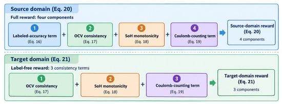
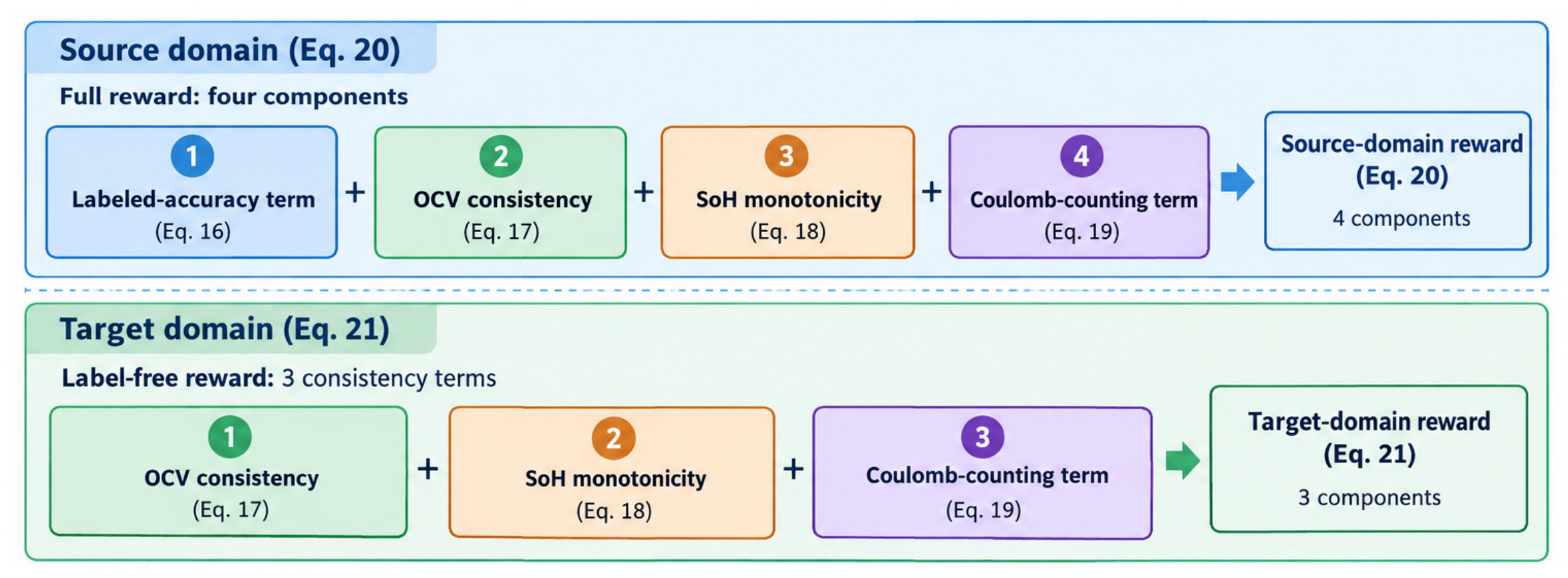
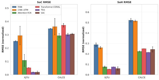
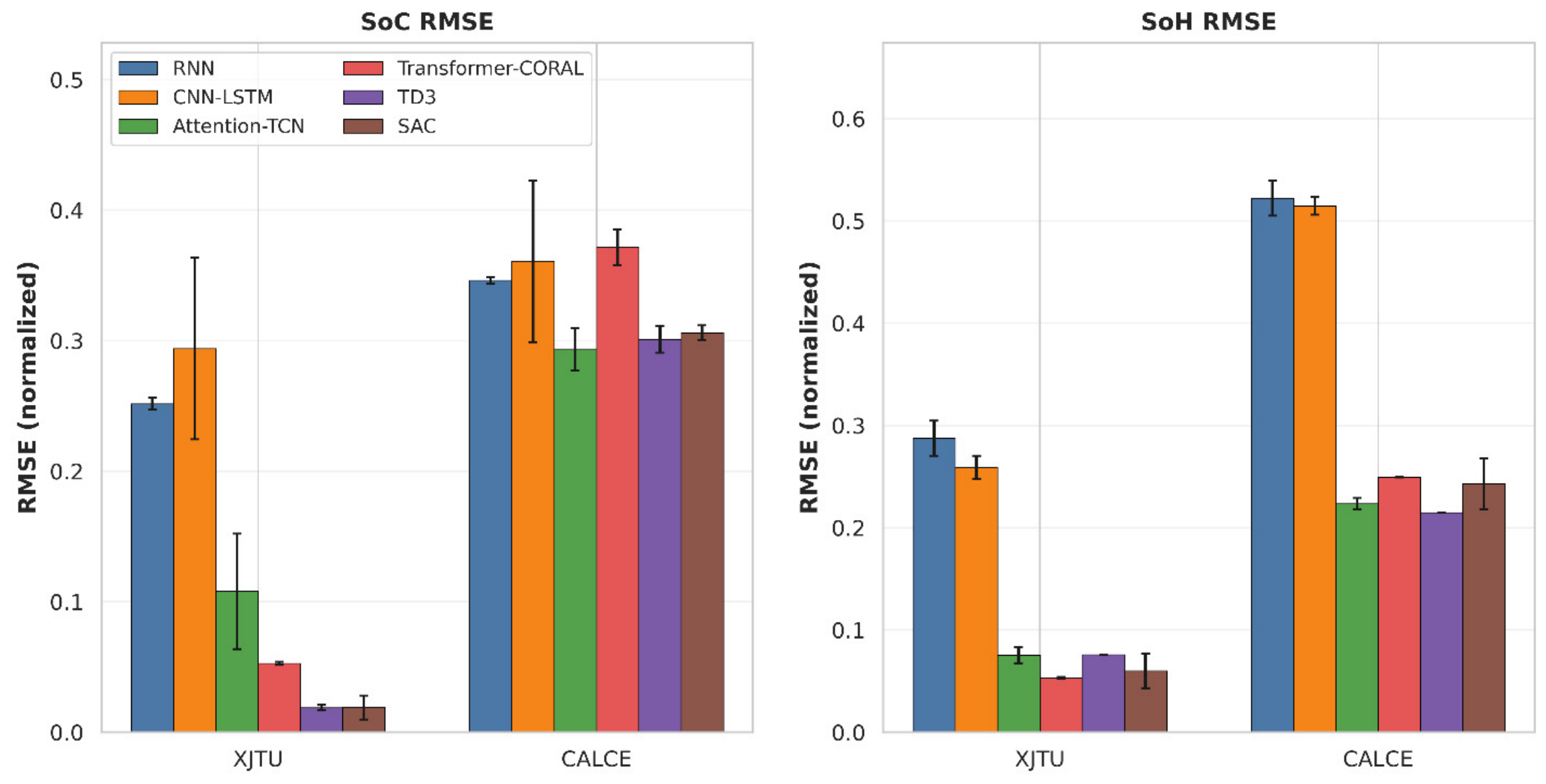
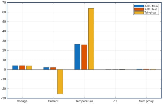
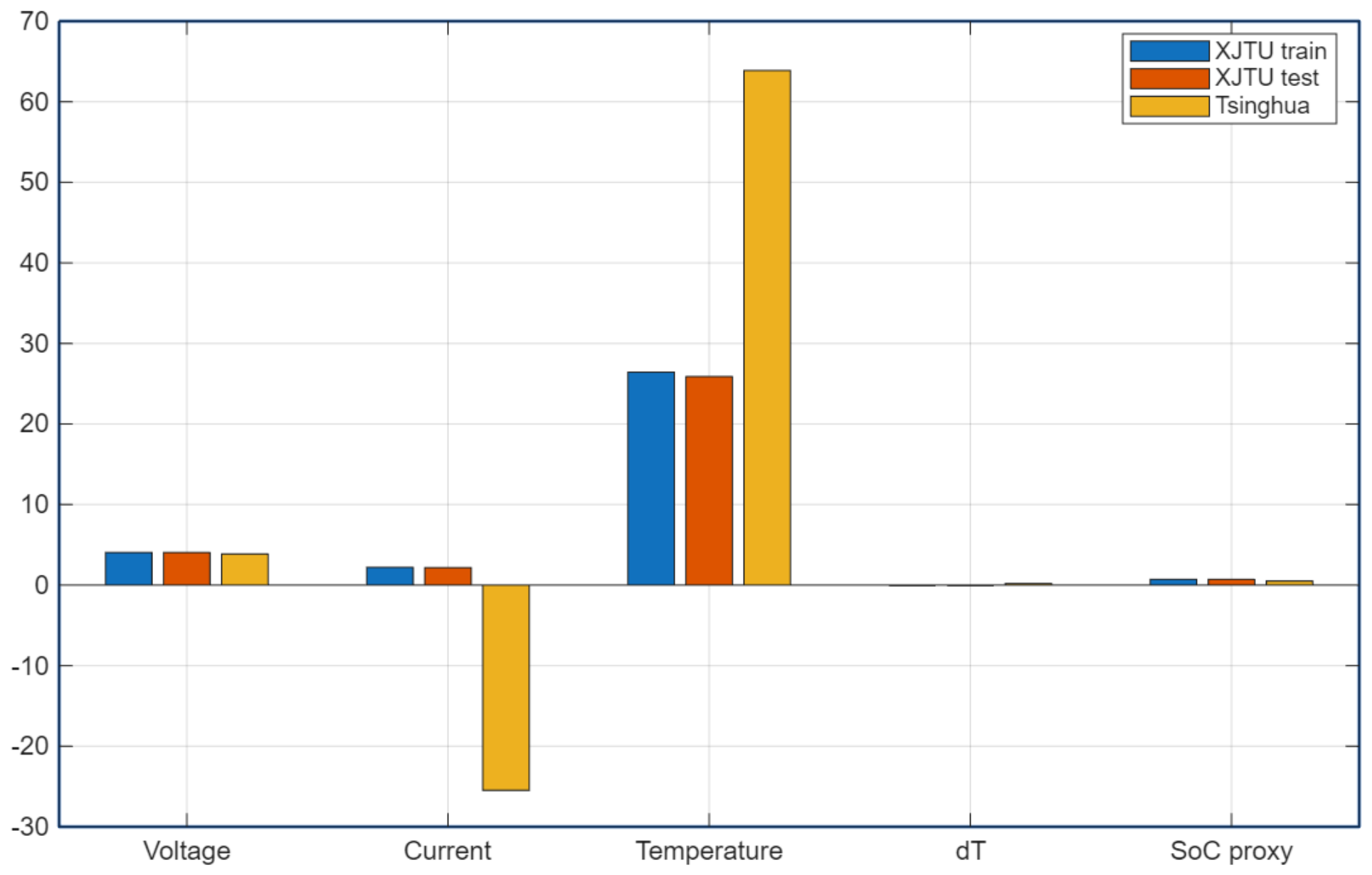
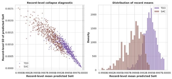
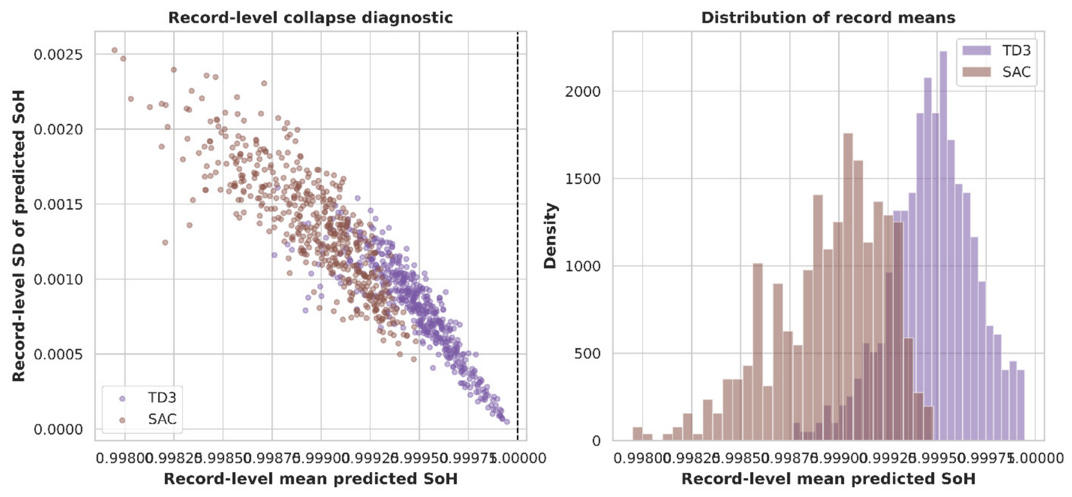
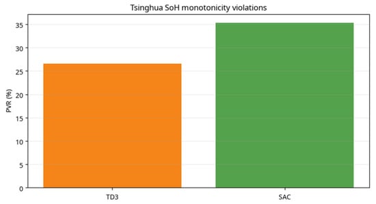
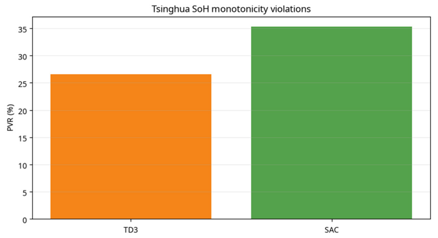
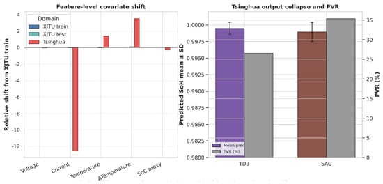
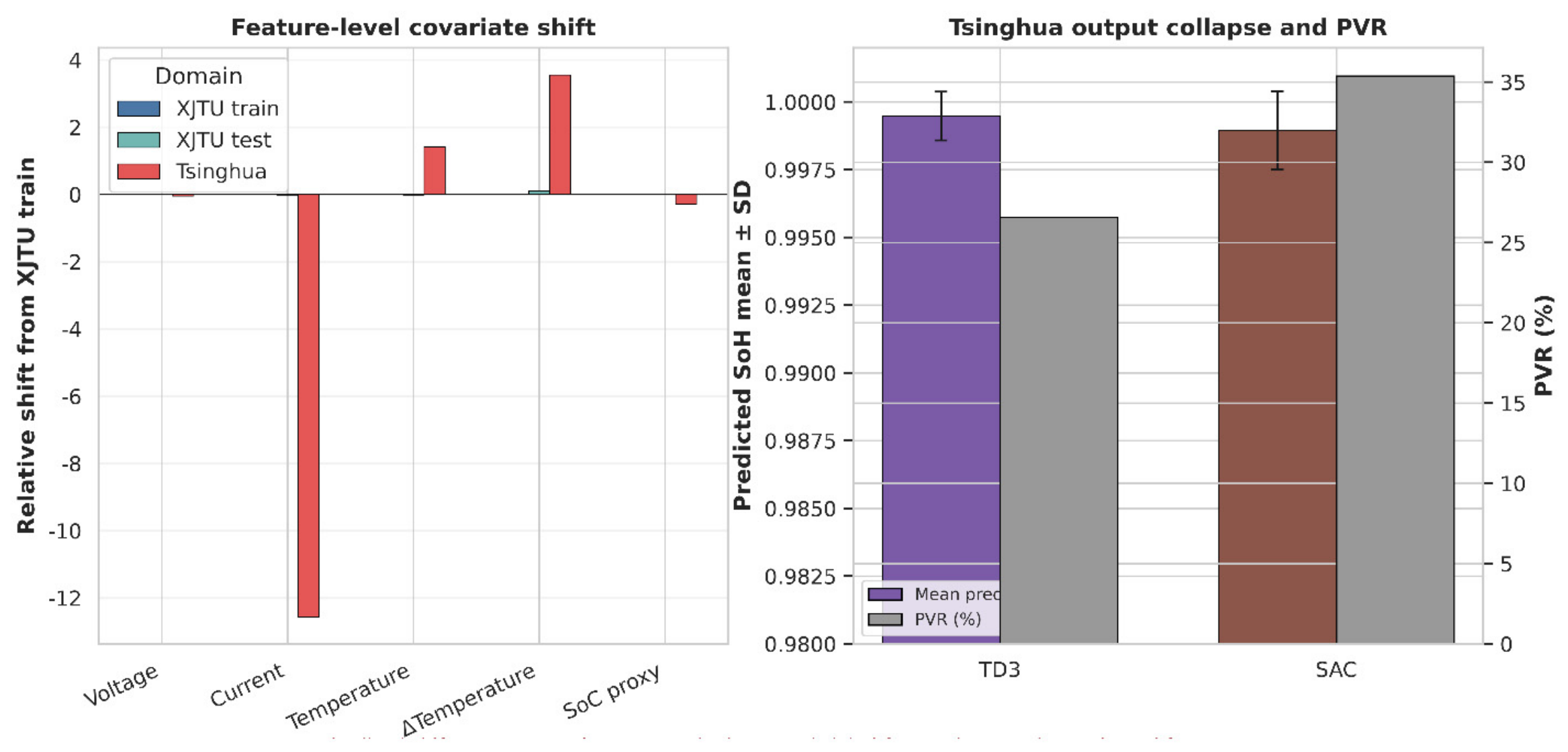

Disclaimer/Publisher’s Note: The statements, opinions and data contained in all publications are solely those of the individual author(s) and contributor(s) and not of MDPI and/or the editor(s). MDPI and/or the editor(s) disclaim responsibility for any injury to people or property resulting from any ideas, methods, instructions or products referred to in the content. |
© 2026 by the authors. Published by MDPI on behalf of the World Electric Vehicle Association. Licensee MDPI, Basel, Switzerland. This article is an open access article distributed under the terms and conditions of the Creative Commons Attribution (CC BY) license.